3.15-seismic design 2008 - illinois department of
TRANSCRIPT
Design Guides 3.15 - Seismic Design
May 2008 Page 3.15-1
3.15 Seismic Design
This design guide focuses on simple and practical techniques which can be used for the
analysis and design of typical bridges in Illinois for earthquake loadings. More sophisticated
methods are not discouraged by the Department given that the designer has the expertise. The
primary format of this guide is to provide examples with discussion and commentary. Example
Bridges No. 1 and No. 4 are the most complete. General guidance is also provided beyond the
scope of the specific example structures for many other bridge types and potential design
scenarios. The intent is to cover as broad a range of subjects as possible in this relatively short
forum. Examples 1, 2 & 3 focus on bridges commonly built on the State and Local Systems.
Examples 2 and 3 either illustrate a variation on Example 1 which requires a demonstration of a
separate set of methods and calculations for clarity, or builds upon concepts already presented.
Example 4 deals with a class of bridges historically constructed on the Local Bridge System,
single and multi-span simply supported PPC deck beam structures. These bridges have some
special characteristics and design considerations (which includes the flexible design option
described in Section 3.15.8 of the Bridge Manual) that are unique compared to other structure
types built in the State. Taken as a whole, this design guide is intended as an abbreviated
primer on the design of typical bridges in Illinois for earthquake loadings.
The design of superstructure-to-substructure connections along with seat widths (Level 1 and
Level 2 Redundancies in the Department’s ERS framework) is straightforward and not covered
in Examples 1 to 3. However, Example 4 does because simply supported PPC deck beam
bridges have some special design considerations for the Level 1 and 2 Redundancies. See
also Sections 3.7 and 3.15 of the Bridge Manual for more information.
This design guide deals with both the 1000 yr. (LRFD) and 500 yr. (LFD) design return period
earthquakes. Both will still be relevant for bridges in Illinois for the foreseeable future with the
importance of the 500 yr. event decreasing over time. Example 1 juxtaposes the seismic design
methods and calculations for an identical bridge for both the 1000 yr. and 500 yr. events in order
to highlight the differences and similarities between the two, and serves as a transitional
reference for the designer. Example 1 also demonstrates that the increases in concrete
member strengths, the number of piles required, etc. when going from the 500 yr. to the 1000
yr. design event are not overly dramatic.

Design Guides 3.15 - Seismic Design
Page 3.15-2 May 2008
The following is an outline of provided examples:
Example 1 3-Span Wide Flange Bridge with Pile Supported Multiple Circular Column Bents, Open Pile Supported Stub Abutments (Pile Bents), and No Skew
1. Determination of Bridge Period – Transverse Direction a. Weight of Bridge for Seismic Calculations
b. Global Transverse Structural Model of the Bridge
c. Transverse Pier Stiffness for Un-cracked and Cracked Columns
d. Transverse Abutment Stiffness
e. Transverse Superstructure Stiffness
f. Uniform Load Method Transverse Period Determination for Un-cracked Columns
g. Uniform Load Method Transverse Period Determination for Cracked Columns
2. Determination of Bridge Period – Longitudinal Direction a. Weight and Global Longitudinal Structural Model of the Bridge b. Longitudinal Pier Stiffness for Un-cracked and Cracked Columns c. Uniform Load Method Longitudinal Period Determination for Un-cracked and
Cracked Columns 3. Determination of Base Shears – 500 Year Design Earthquake Return Period
a. Design Response Spectrum (LFD) b. Transverse Base Shear c. Longitudinal Base Shear
4. Determination of Base Shears – 1000 Year Design Earthquake Return Period a. Design Response Spectrum (LRFD) b. Transverse Base Shear c. Longitudinal Base Shear
5. Frame Analysis and Columnar Seismic Forces for Multiple Column Bent – 500 and 1000 Year Design Earthquake Return Period
a. Pier Forces – Dead Load b. Pier Forces – Transverse Overturning c. Pier Forces – Transverse Frame Action d. Pier Forces – Longitudinal Cantilever

Design Guides 3.15 - Seismic Design
May 2008 Page 3.15-3
6. Seismic Design Forces for Multiple Column Bent Including R-Factor, P-Δ, and Combination of Orthogonal Forces – 500 and 1000 Year Design Earthquake Return Period
a. R-Factor
b. P-Δ
c. Summary and Combination of Orthogonal Column Forces Used for Design
7. Column Design Including Overstrength Plastic Moment Capacity – 500 and 1000
Year Design Earthquake Return Period a. Column Design for Axial Force and Moment
b. Column Design for Shear
c. 1000 Year Return Period Plastic Shear Determination Using Overstrength
8. Pile Design Overview
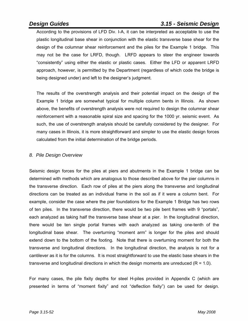
Example 2 Example 1 Bridge with a Skew of 30° for the 500 Year Design Earthquake Return Period
1. Determination of Bridge Periods and Base Shears – 500 Year Design
Earthquake Return Period
2. Frame Analysis and Columnar Seismic Forces for Multiple Column Bent – 500
Year Design Earthquake Return Period a. Pier Forces – Dead Load
b. Pier Forces from Global Transverse Base Shear
c. Pier Forces from Global Longitudinal Base Shear
3. Seismic Design Forces for Multiple Column Bent Including R-Factor, P-Δ, and
Combination of Orthogonal Forces – 500 Year Design Earthquake Return Period a. R-Factor
b. P-Δ
c. Summary and Combination of Orthogonal Column Forces Used for Design
Design Guides 3.15 - Seismic Design
Page 3.15-4 May 2008
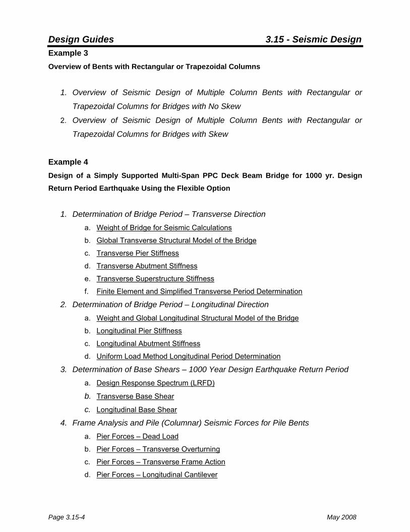
Example 3 Overview of Bents with Rectangular or Trapezoidal Columns
1. Overview of Seismic Design of Multiple Column Bents with Rectangular or
Trapezoidal Columns for Bridges with No Skew
2. Overview of Seismic Design of Multiple Column Bents with Rectangular or
Trapezoidal Columns for Bridges with Skew
Example 4 Design of a Simply Supported Multi-Span PPC Deck Beam Bridge for 1000 yr. Design Return Period Earthquake Using the Flexible Option
1. Determination of Bridge Period – Transverse Direction a. Weight of Bridge for Seismic Calculations
b. Global Transverse Structural Model of the Bridge
c. Transverse Pier Stiffness
d. Transverse Abutment Stiffness
e. Transverse Superstructure Stiffness
f. Finite Element and Simplified Transverse Period Determination
2. Determination of Bridge Period – Longitudinal Direction a. Weight and Global Longitudinal Structural Model of the Bridge
b. Longitudinal Pier Stiffness
c. Longitudinal Abutment Stiffness
d. Uniform Load Method Longitudinal Period Determination
3. Determination of Base Shears – 1000 Year Design Earthquake Return Period a. Design Response Spectrum (LRFD)
b. Transverse Base Shear
c. Longitudinal Base Shear
4. Frame Analysis and Pile (Columnar) Seismic Forces for Pile Bents a. Pier Forces – Dead Load
b. Pier Forces – Transverse Overturning
c. Pier Forces – Transverse Frame Action
d. Pier Forces – Longitudinal Cantilever

Design Guides 3.15 - Seismic Design
May 2008 Page 3.15-5
5. Frame Analysis and Pile (Columnar) Seismic Forces for Abutments a. Abutment Forces – Dead Load
b. Abutment Forces – Transverse Overturning
c. Abutment Forces – Transverse Frame Action
d. Abutment Forces – Longitudinal Cantilever
6. Seismic Design Forces for Pile Bent Including R-Factor, P-Δ, and Combination of
Orthogonal Forces a. R-Factor
b. P-Δ
c. Summary and Combination of Orthogonal Column Forces Used for Design
7. Seismic Design Forces for Abutment Including R-Factor, P-Δ, and Combination
of Orthogonal Forces a. R-Factor
b. P-Δ
c. Summary and Combination of Orthogonal Column Forces Used for Design
8. Combined Axial Force and Bi-Axial Bending Structural Capacity Check for Piles
in Bents a. Load Case 1 – Longitudinal Dominant
b. Load Case 2 – Transverse Dominant
9. Combined Axial Force and Bi-Axial Bending Structural Capacity Check for Piles
in Abutments a. Load Case 1 – Longitudinal Dominant
b. Load Case 2 – Transverse Dominant
10. Discussion of Flexible Versus Standard Design Options
11. Pile Shear Structural Capacity Check, and Pile Connection Details, and Cap
Reinforcement Details a. Shear Capacity Check of HP Piles
b. Anchorage Details at Piers and Abutments for HP Piles
c. Added Pier Cap Confinement Reinforcement
12. Dowel Bar Connection of Beams to Pier and Abutment Caps
13. Minimum Support Length (Seat Width) Requirements at Piers and Abutments
14. Overview of Example Bridge Design With Metal Shell Piles

Design Guides 3.15 - Seismic Design
Page 3.15-6 May 2008
a. Determination of Bridge Periods and Base Shears – Transverse and Longitudinal
Directions
b. Frame Analysis and Seismic Design Forces for Piers and Abutments
c. Combined Axial Force and Bending Structural Capacity Check for Piers and
Abutments
d. Pile Shear Structural Capacity Check, Minimum Steel, and Pile Connection
Details
e. Pier Cap Reinforcement, Connection of Beams to Pier and Abutment Caps, and
Support Length

Design Guides 3.15 - Seismic Design
May 2008 Page 3.15-7
Example 1 3-Span Wide Flange Bridge with Pile Supported Multiple Circular Column Bents, Open Pile Supported Stub Abutments (Pile Bents), and No Skew
62 ft. 77 ft. 62 ft.
E F E E
62 ft. 77 ft. 62 ft.
E F E E
42 ft.
6 spaces @ 6 ft. = 36 ft.
7 ½ in. 1 ½ in. Added Surface13
42 ft.
6 spaces @ 6 ft. = 36 ft.
7 ½ in. 1 ½ in. Added Surface13
12 ft. –6 in. 2 ft. – 6 in.
42 ft.
4 ft.
4 ft.2 ft. – 3 in.
12 ft.12 ft. –6 in. 2 ft. – 6 in.
42 ft.
4 ft.
4 ft.2 ft. – 3 in.
12 ft.
62 ft. 77 ft. 62 ft.
E F E E
62 ft. 77 ft. 62 ft.
E F E E
42 ft.
6 spaces @ 6 ft. = 36 ft.
7 ½ in. 1 ½ in. Added Surface13
42 ft.
6 spaces @ 6 ft. = 36 ft.
7 ½ in. 1 ½ in. Added Surface13
12 ft. –6 in. 2 ft. – 6 in.
42 ft.
4 ft.
4 ft.2 ft. – 3 in.
12 ft.12 ft. –6 in. 2 ft. – 6 in.
42 ft.
4 ft.
4 ft.2 ft. – 3 in.
12 ft.
Beams W36 x 170; ksi 29000E ksi; 3372E ksi; 36f psi; 3500f scy'c ====
1. Determination of Bridge Period – Transverse Direction
1.a. Weight of Bridge for Seismic Calculations
The mass (weight) of a bridge used for seismic design is usually computed first. The mass
to consider is that portion of the superstructure and substructures which can reasonably be
expected to accelerate horizontally during an earthquake. The total weight of the
superstructure including any cross bracing, diaphragms, and parapets should always be
included along with the weight of the cap beams and half the columns or walls at piers. In
this example, the abutments do not have a reasonable expectation of accelerating to any
great degree and are not included. If a bridge has integral abutments, the weight of the end
diaphragms should be included (bottom of deck to bottom of bearings). Future wearing
surface (“Added Surface” in the figure above) can be added to the weight of a bridge
considered for seismic design at the designer’s discretion. The total calculated weight can
Design Guides 3.15 - Seismic Design
Page 3.15-8 May 2008
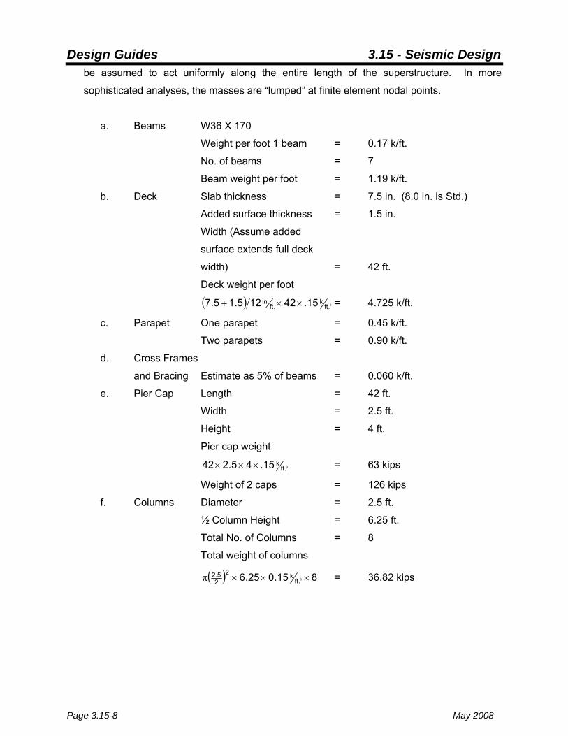
be assumed to act uniformly along the entire length of the superstructure. In more
sophisticated analyses, the masses are “lumped” at finite element nodal points.
a. Beams W36 X 170
Weight per foot 1 beam = 0.17 k/ft.
No. of beams = 7
Beam weight per foot = 1.19 k/ft.
b. Deck Slab thickness = 7.5 in. (8.0 in. is Std.)
Added surface thickness = 1.5 in.
Width (Assume added
surface extends full deck
width) = 42 ft.
Deck weight per foot
( ) 3.ftk
.ft.in 15.42125.15.7 ××+ = 4.725 k/ft.
c. Parapet One parapet = 0.45 k/ft.
Two parapets = 0.90 k/ft.
d. Cross Frames
and Bracing Estimate as 5% of beams = 0.060 k/ft.
e. Pier Cap Length = 42 ft.
Width = 2.5 ft.
Height = 4 ft.
Pier cap weight
3.ftk15.45.242 ××× = 63 kips
Weight of 2 caps = 126 kips
f. Columns Diameter = 2.5 ft.
½ Column Height = 6.25 ft.
Total No. of Columns = 8
Total weight of columns
( ) 815.025.6 3.ftk2
25.2 ×××π = 36.82 kips

Design Guides 3.15 - Seismic Design
May 2008 Page 3.15-9
g. Total Weight Length of Bridge = 201 ft.
a. + b. + c. + d. = 6.875 k/ft.
or a. + b. + c. + d. = 1381.875 kips
e. + f. = 162.82 kips
Total Weight = 1544.7 kips
1.b. Global Transverse Structural Model of the Bridge
Very simple or more complex global structural models of bridges for dynamic and equivalent
static analyses can be used at the designer’s discretion. For many typical bridges in Illinois,
models that tend to be fairly simple produce reasonable and adequate results for seismic
design. Shown below is the global analysis model used for the current example.
kAbut kAbutkPier kPier
ITransverse Superstructure
62 ft. = 744 in. 77 ft. = 924 in. 62 ft. = 744 in.
201 ft. = 2412 in.
kAbut kAbutkPier kPier
ITransverse Superstructure
62 ft. = 744 in. 77 ft. = 924 in. 62 ft. = 744 in.
201 ft. = 2412 in.
Methods for the determination of superstructure, pier and abutment stiffnesses (moment of
inertia and spring constants) are given below. At a minimum, the simplest global model
should include the stiffnesses of the superstructure and piers with the abutments pinned.
Simplification to this level, however, is not recommended but still acceptable. The Uniform
Load Method of Analysis, which is advocated by the Department, tends to over estimate
reactions at the abutments. Assigning stiffness to the abutments, as opposed to pinned
supports that are rigid for transverse displacement, produces more accurate results when
using the Uniform Load Method.
The current example bridge can be straightforwardly analyzed with hand methods largely
because there are not more than 3 spans and the structure is “very symmetric”. For cases

Design Guides 3.15 - Seismic Design
Page 3.15-10 May 2008
where bridges are not symmetric, simple finite element models of the same type shown
above can be used for the analysis. If desired, spring finite elements can also be replaced
with axial force/truss elements with an equivalent spring stiffness based upon k =
(Area)(Mod. of Elasticity)/(Length).
For most cases, the (fundamental) period of the “first mode of vibration” is typically all that
needs to be computed because it dominates the dynamic displacement response of a bridge
(i.e. multi-modal analysis is not required for typical or regular bridges). The displaced
“shape” of the first mode generally approximates that of a half sine wave. This shape will be
apparent in subsequent sections below when the fundamental periods of the Example 1
bridge with un-cracked and cracked pier sections are calculated. The second mode of
vibration will tend to approximate a full sine wave, the third 1 ½ sine waves, etc. In complex
dynamic analyses which use finite elements and time as a variable, the “equations of
motion” are coupled together and difficult to solve in the time domain. Transforming the
equations of motion and responses of a structure into the frequency domain uncouples them
in such a way that the equations become “solvable”. Solutions in the frequency domain, at
any point in time, essentially can be thought of as giving the relative magnitude of
importance each mode has in the total displacement. For many structures, the first mode
dominates the solutions and, as such, the responses from higher modes can be neglected
for engineering design purposes.
1.c. Transverse Pier Stiffness for Un-cracked and Cracked Columns
For multiple column bent piers, the columns are considered to be the “weak link” or 3rd tier
seismic fuse according to IDOT’s ERS plan. It should be assumed that the columns deflect
in reverse curvature with fixed ends at the bottom of the cap and the top of the crashwall
(clear height). The equations below determine the stiffness.
Column Moment of Inertia diameter column where; 4
2I col
4col
c =φ⎟⎠⎞
⎜⎝⎛φπ
=
Column Stiffness height column clearh where; h
IE12k c3
c
ccc =
××=

Design Guides 3.15 - Seismic Design
May 2008 Page 3.15-11
For a simple analysis, the foundation should be assumed fixed. When the piles are sized,
the seismic design forces used will typically be unreduced by an R-Factor (designed
elastically). So, the foundation will be significantly stiffer than the columns in the piers.
For the 500 year design earthquake return period event, the columns may be assumed to be
“un-cracked”. At the 1000 year level, the columns should be considered cracked with an
effective moment of inertia of ½ that of Ic. The stiffness of the piers for the current example
is given below.
Column Moment of Inertia ( ) 44
c in. 8.397604
in. 15 I =×π
=
Cracked Moment of Inertia 442/c in. 4.198802
in. 8.39760I ==
Clear Height of Column 12.5 ft. = 150 in.
Concrete Modulus of Elasticity Ec = 3372 ksi
Stiffness of Un-cracked Column in.k
3c 7.476 150
8.39760337212k =××
=
Stiffness of Cracked Column in.kin.
kc 4.2382
7.476k ==
Stiffness of Un-cracked Pier in.k
in.k
Pier 8.1906columns 4 7.476k =×=
Stiffness of Cracked Pier in.k
in.k
Pier 6.953columns 4 4.238k =×=
Notes for Other Pier Types: Similar calculations to those above can also be used to
determine the transverse stiffness of individual column drilled shaft bents, solid wall encased
drilled shaft bents, drilled shaft bents with crashwalls, individually encased pile bents, solid
wall encased pile bents, solid wall piers supported by a footing and piles, modified
hammerhead piers supported by a footing and piles, and trapezoidal multiple column bents
with crashwalls. In addition, at the designer’s discretion, hammerhead piers may be
analyzed as a single column in reverse curvature above ground with similar techniques to
those used above.
The “clear height” of individual column drilled shaft bents and individually encased pile bents
should be taken from the depth-of-fixity in the soil to the bottom of the cap beam. The clear

Design Guides 3.15 - Seismic Design
Page 3.15-12 May 2008
height for solid wall encased drilled shaft bents and solid wall encased pile bents should be
from the depth-of-fixity to the bottom of the solid wall encasement. The walls are assumed
to be rigid links in the transverse direction (or a deep cap beam). The clear column height
for drilled shaft bents with a crashwall and trapezoidal column bents with crashwall is the
same as that for the current example with the drilled shafts below the wall or the piles below
the footing assumed fixed. The clear column height of solid wall and modified hammerhead
piers supported by a footing and piles should be taken from the depth-of-fixity to the bottom
of the footing. The walls and footings are assumed to be rigid links for these two cases.
The clear column height for hammerhead piers can be taken from the bottom of the
cantilevered cap to the top of the footing at the designer’s discretion. Hammerheads can
tend to behave somewhat as a single column pier as opposed to a wall.
Methods for dealing with the added complexities of skew, and skew in combination with
cross-sections which are not round are given in Examples 2 and 3.
1.d. Transverse Abutment Stiffness
In this example, the stiffness of the abutments will be calculated assuming only the steel H-
piles contribute. The piles can be modeled as individual columns in soil in reverse curvature
with a clear height extending from the depth-of-fixity in the soil to the bottom of the abutment
cap. Batter in the piles for situations such as the current example can be ignored. The
designer may also consider the stiffness provided by the abutment and wings bearing on the
soil or any other sources of stiffness judged appropriate. For example, integral abutments
may be modeled with an additional rotational spring which simulates the stiffness of the
diaphragm. For most cases, though, this is not necessary or recommended. The stiffness of
the abutments for the current example is given below.
Piles HP 12 x 74
Number of Piles 9
Weak Axis Pile Moment of Inertia Ip = 186 in.4
(Typical Orientation for Illinois)
Steel Modulus of Elasticity Es = 29000 ksi
Pile Effective Height 8.0 ft. = 96.0 in.
(from Geotechnical Analysis-

Design Guides 3.15 - Seismic Design
May 2008 Page 3.15-13
see also Appendix C)
Stiffness of Abutment h
IE12 piles) .no(k 3
p
psAbut
×××=
in.k
3Abut 4.6580.96
1862900012 9k =×××
=
1.e. Transverse Superstructure Stiffness
During an earthquake, the superstructure deflects horizontally as one “effective beam”. The
deck and beams are the primary contributors to the moment of inertia. The parapets may or
may not be considered to contribute to the superstructure moment of inertia. For typical
IDOT bridges, it may be most realistic to consider the parapets half effective. Future
wearing surface should not be considered to contribute to the superstructure moment of
inertia. “Shear lag” in the beams should always be accounted for by considering them half
effective. The beam areas “lag” in effectiveness for resisting horizontal loads as the
distance from the deck increases. For the current example, the parapets have been
assumed to be fully effective. The superstructure moment of inertia calculations are given
below.
Es 29000 ksi
Ec 3372 ksi
n (modular ratio) 8.6
Slab Thickness 7.5 in.
Slab Width 42 ft.
Slab Moment of Inertia ( ) 473ft.
in.121
slab .in 100.812ft. 425.7I ×=×××=
Area of 1 Parapet 432 in.2
Area of 1 Beam 50 in.2
Transformed Beam Area ( ) 2steel in. 215
2506.8
Lag Shear for 2Beam 1 AreanA =
×=
×=

Design Guides 3.15 - Seismic Design
Page 3.15-14 May 2008
480 in.
6 spaces @ 6 ft. = 36 ft.
13
Bm.2
Bm.3
Bm.1
Bm.1
Bm.2
Bm.3
480 in.
6 spaces @ 6 ft. = 36 ft.
13
Bm.2
Bm.3
Bm.1
Bm.1
Bm.2
Bm.3
Moment of Inertia of Superstructure Table
No. I0 (In4) A (in2) I (in4)
Parapet 2 ---- 432 240 2.49E+07 4.98E+07Slab 1 8.00E+07 ---- ---- ---- 8.00E+07
Beam 1 2 ---- 215 72 1.11E+06 2.23E+06Beam 2 2 ---- 215 144 4.46E+06 8.92E+06Beam 3 2 ---- 215 216 1.00E+07 2.01E+07
ITotal 1.610E+08 in4
(in) x )(in xA 42×
1.f. Uniform Load Method Transverse Period Determination for Un-cracked Columns
The first step in the method is to calculate the maximum displacement of the bridge for a
simple uniform load, usually 1 k/in. or 1 k/ft. The maximum displacement in this example will
occur at the center of the structure. If a bridge has asymmetries such as unequal span
lengths, or piers and abutments with different stiffnesses; the maximum deflection will occur
somewhere other than the center of the structure. The total uniform load applied to the
structure is divided by the maximum deflection to determine an equivalent very simple
bridge stiffness. The equivalent stiffness encompasses the effects of the superstructure,
abutment and pier stiffnesses. The period is a function of the weight of the structure
(determined above) and the equivalent stiffness using a basic equation from structural
dynamics. The calculations for the period of the Example 1 bridge are given below with
hand methods for piers which are un-cracked. The period for cracked analysis is also given
with minimal calculations shown as the method for period determination is the same with
different pier stiffnesses.

Design Guides 3.15 - Seismic Design
May 2008 Page 3.15-15
a. Find the deflection of the bridge for a uniform load of 1 k/in. assuming there are
no piers and the abutments are infinitely stiff (deflection of a simple beam).
w (uniform load) 1 k/in.
L (bridge length) 201 ft. = 2412 in.
Ec 3372 in.2
ITotal 1.61 x 108 in.4
Deflection Totalc
4
c IE384Lw5
××××
=δ
.in 812.01610000003372384
241215 4
c =××
××=δ
b. Find the deflection of the bridge for a uniform load of 1 k/in. assuming no piers,
an infinitely stiff superstructure and abutment springs (simple deflection of a pair
of springs).
w (uniform load) 1 k/in.
L (bridge length) 201 ft. = 2412 in.
kAbut 658.4 k/in.
Deflection Abut
e k2
Lw ×
=δ
in. 832.14.658224121
e =
×
=δ
c. Total deflection for a uniform load of 1 k/in. without piers considered.
0.812 in.
1.383 in.
Total Deflection in. 644.2ecT =δ+δ=δ

Design Guides 3.15 - Seismic Design
Page 3.15-16 May 2008
d. Find the estimated deflection at the center of the bridge for a point load, P, at
each pier location without considering pier stiffness and with infinitely stiff
abutments.
a and x
L
a and xL – 2a
P P
δvc
a and x
L
a and xL – 2a
P P
δvc
L 2412 in.
x 744 in.
a 744 in.
Ec 3372 ksi
ITotal 1.61 x 108 in.4
Deflection ( )22
Totalcvc a4L3
IE24aP
×−×××
×=δ
( )22vc 744424123
161000000337224744P
×−××××
=δ
P0008702.0vc =δ
e. Find the estimated deflection at the pier locations for a point load, P, at each pier
location without considering pier stiffness and with infinitely stiff abutments.
a and x
L
a and xL – 2a
P P
δvp
a and x
L
a and xL – 2a
P P
δvp
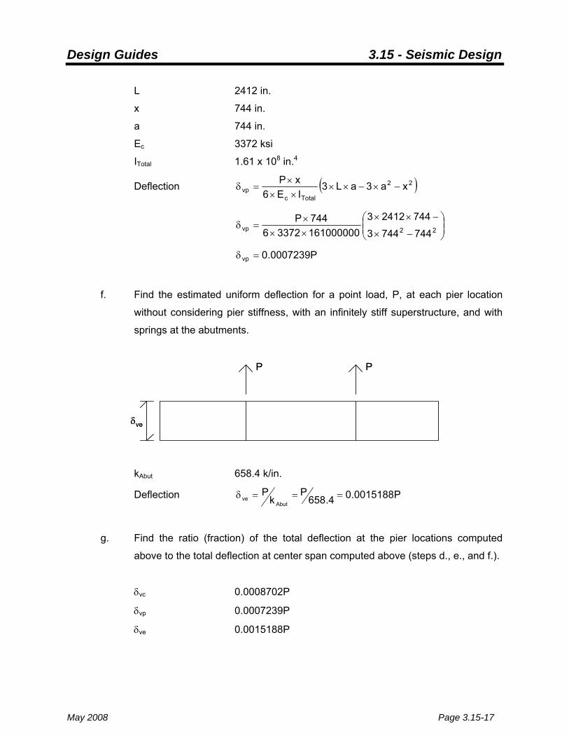
Design Guides 3.15 - Seismic Design
May 2008 Page 3.15-17
L 2412 in.
x 744 in.
a 744 in.
Ec 3372 ksi
ITotal 1.61 x 108 in.4
Deflection ( )22
Totalcvp xa3aL3
IE6xP
−×−××××
×=δ
⎟⎟⎠
⎞⎜⎜⎝
⎛
−×
−××
×××
=δ 22vp 744744374424123
16100000033726744P
P0007239.0vp =δ
f. Find the estimated uniform deflection for a point load, P, at each pier location
without considering pier stiffness, with an infinitely stiff superstructure, and with
springs at the abutments.
P P
δve
P P
δve
kAbut 658.4 k/in.
Deflection P0015188.04.658P
kP
Abutve ===δ
g. Find the ratio (fraction) of the total deflection at the pier locations computed
above to the total deflection at center span computed above (steps d., e., and f.).
δvc 0.0008702P
δvp 0.0007239P
δve 0.0015188P
Design Guides 3.15 - Seismic Design
Page 3.15-18 May 2008
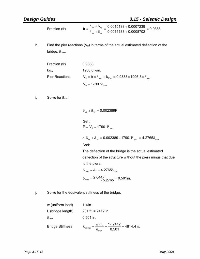
Fraction (fr) 9388.00008702.00015188.00007239.00015188.0fr
vcve
vpve =++
=δ+δ
δ+δ=
h. Find the pier reactions (V0) in terms of the actual estimated deflection of the
bridge, δmax.
Fraction (fr) 0.9388
kPier 1906.8 k/in.
Pier Reactions maxPiermax0 8.19069388.0kfrV δ××=×δ×=
max0 1.1790V δ=
i. Solve for δmax
maxmaxvcve
max0
vcve
2765.41.1790002389.0
1.1790VP:Set
P002389.0
δ=δ×=δ+δ∴
δ==
=δ+δ
And:
The deflection of the bridge is the actual estimated
deflection of the structure without the piers minus that due
to the piers.
maxTmax 2765.4 δ−δ=δ
in. 501.02765.5644.2
max ==δ
j. Solve for the equivalent stiffness of the bridge.
w (uniform load) 1 k/in.
L (bridge length) 201 ft. = 2412 in.
δmax 0.501 in.
Bridge Stiffness in.k
maxBridge 4.4814
501.024121Lwk =
×=
δ×
=

Design Guides 3.15 - Seismic Design
May 2008 Page 3.15-19
k. Solve for the period of the bridge.
Total Weight 1544.7 kips
Accel. of Gravity (g) 386.4 in./sec.2
Bridge Stiffness 4814.4 k/in.
Period (T) sec. 18.04.48144.386
7.15442kgW2T
Bridge
=×
π=×
π=
1.g. Uniform Load Method Transverse Period Determination for Cracked Columns
In order to compute the period of the bridge with cracked columns, steps h. through k. from
above need only be repeated.
h. Find the pier reactions (V0) in terms of the actual estimated deflection of the
bridge, δmax.
Fraction (fr) 0.9388
kPier 953.6 k/in.
Pier Reactions maxPiermax0 6.9539388.0kfrV δ××=×δ×=
max0 2.895V δ=
i. Solve for δmax.
maxmaxvcve
max0
vcve
1386.22.895002389.0
2.895VP:Set
P002389.0
δ=δ×=δ+δ∴
δ==
=δ+δ
And:
The deflection of the bridge is the actual estimated
deflection of the structure without the piers minus that due

Design Guides 3.15 - Seismic Design
Page 3.15-20 May 2008
to the piers.
maxTmax 1386.2 δ−δ=δ
in. 842.01386.3644.2
max ==δ
j. Solve for the equivalent stiffness of the bridge.
w (uniform load) 1 k/in.
L (bridge length) 201 ft. = 2412 in.
δmax 0.842 in.
Bridge Stiffness in.k
maxBridge 6.2864
842.024121Lwk =
×=
δ×
=
k. Solve for the period of the bridge.
Total Weight 1544.7 kips
Accel. of Gravity (g) 386.4 in./sec.2
Bridge Stiffness 2864.6 k/in.
Period (T) sec. 23.06.28644.386
7.15442kgW2T
Bridge
=×
π=×
π=
When the columns are cracked, the period of the bridge increased from 0.18 sec. to 0.23
sec. or about 28% greater than the un-cracked case. This is because the superstructure
stiffness is dominant which is typical of many Illinois bridges. It is also somewhat unusual
for the transverse period of a typical bridge in Illinois to be near 1.0 sec. Consequently, if a
long (around 0.75 sec. and greater) transverse period is calculated, there may either be an
error in the designer’s calculations or the bridge may not be modeled properly.
Design Guides 3.15 - Seismic Design
May 2008 Page 3.15-21
2. Determination of Bridge Period – Longitudinal Direction
2.a. Weight and Global Longitudinal Structural Model of the Bridge The mass of the bridge used for calculation of the longitudinal period is the same as that
calculated above for the transverse direction. For this example, the piers are assumed to be
the only elements of the bridge which contribute stiffness to the longitudinal period. The
superstructure acts as a rigid link between the two piers with the abutments assumed to
provide no resistance to seismic load.
It is also acceptable and/or more correct to consider that the abutments contribute to the
stiffness of the bridge in the longitudinal direction depending on the structure configuration.
For example, if the abutments are integral, at a minimum, the stiffness of the piles should be
part of the longitudinal global model. If the abutments are not integral, the designer may
consider the resistance of the beams bearing against a backwall and the soil behind it for
one abutment, or the resistance of the piles, or both. It is also acceptable to consider the
abutments not contributing to the stiffness in the longitudinal direction even if the bearings
are “fixed” but the abutment is an open stub type (pile bent). Making this choice implies that
the designer is “relying” upon the piers to a greater extent than the abutments for resistance
of seismic forces in the longitudinal direction. If adequate seat widths are provided at the
abutments according the 2nd tier of seismic redundancy in IDOT’s ERS strategy, this method
just ensures a more conservative pier design in the longitudinal direction.
2.b. Longitudinal Pier Stiffness for Un-cracked and Cracked Columns
The columns for multiple circular column bents with cap beams should be assumed to
deflect as cantilevers which deform from fixed ends at the top of the crashwall to the bottom
of the cap. The rigid body rotation of the cap should also be included in the stiffness
determination. The equations and derivation below determine the stiffness, and the figure
provides an illustration for guidance.
Column Moment of Inertia diameter column where; 4
2I col
4col
c =φ⎟⎠⎞
⎜⎝⎛φπ
=
Design Guides 3.15 - Seismic Design
Page 3.15-22 May 2008
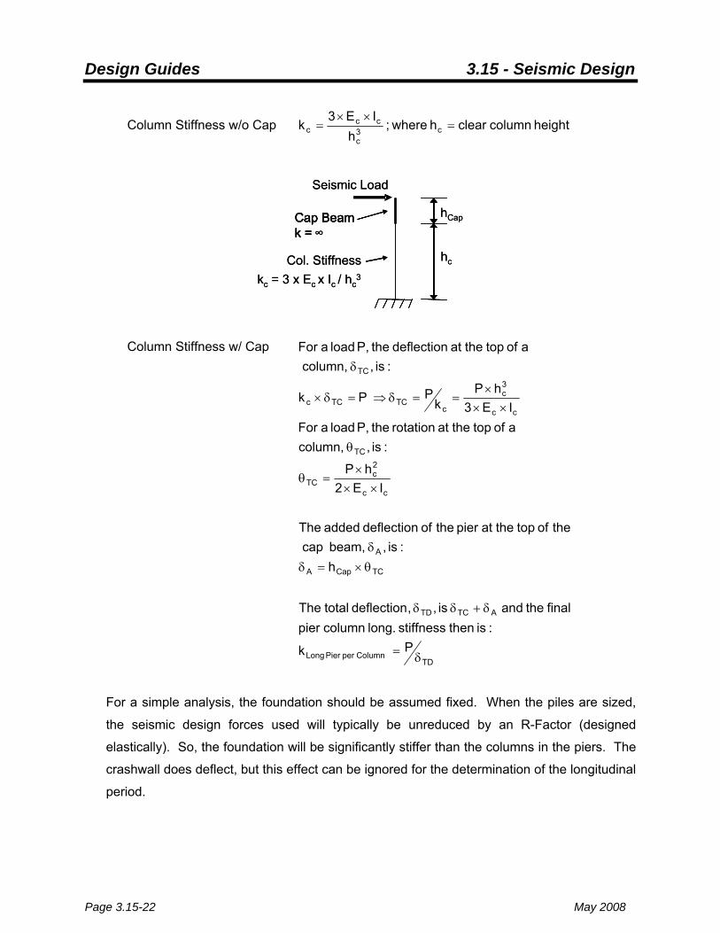
Column Stiffness w/o Cap height column clearh where; h
IE3k c3
c
ccc =
××=
kc = 3 x Ec x Ic / hc3
hc
hCapCap Beamk = ∞
Col. Stiffness
Cap Beamk =
Seismic Load
kc = 3 x Ec x Ic / hc3
hc
hCapCap Beamk = ∞
Col. Stiffness
Cap Beamk =
Seismic Load
Column Stiffness w/ Cap
For a simple analysis, the foundation should be assumed fixed. When the piles are sized,
the seismic design forces used will typically be unreduced by an R-Factor (designed
elastically). So, the foundation will be significantly stiffer than the columns in the piers. The
crashwall does deflect, but this effect can be ignored for the determination of the longitudinal
period.
TD Column per Pier Long
ATCTD
TCCapA
A
cc
2c
TC
TC
cc
3c
cTCTCc
TC
Pk
:is then stiffness long. column pierfinal the and is , ,deflection total The
h:is , beam, cap
the of top the at pier the of deflection added The
IE2hP
:is , column, a of top the at rotation the P, load a For
IE3hP
kP Pk
:is , column, a of top the at deflection the P, load a For
δ=
δ+δδ
θ×=δδ
×××
=θ
θ
×××
==δ⇒=δ×
δ

Design Guides 3.15 - Seismic Design
May 2008 Page 3.15-23
For the 500 year design earthquake return period event, the columns may be assumed to be
“un-cracked”. At the 1000 year level, the columns should be considered cracked with an
effective moment of inertia of ½ that of Ic. The stiffness of the piers for the current example
is given below.
Column Moment of Inertia ( ) 44
c in. 8.397604
in. 15 I =×π
=
Cracked Moment of Inertia 442/c in. 4.198802
in. 8.39760I ==
Clear Height of Column 12.5 ft. = 150 in.
Concrete Modulus of Elasticity Ec = 3372 ksi
Stiffness of Un-cracked Column in.k
3c 2.119 150
8.3976033723k =××
=
Stiffness of Cracked Column in.kin.
kc 6.592
2.119k ==
Stiffness of Un-cracked Column
w/ Cap
Stiffness of Un-cracked Pier in.k
in.k
Pier 0.322columns 4 5.80k =×=
Stiffness of Cracked Pier in.kin.
kPier 161.02
0.322k ==
Notes for Other Pier Types: Similar calculations to those above can also be used to
determine the longitudinal stiffness of individual column drilled shaft bents, solid wall
in.k
TD Column per Pier Long
ATCTD
TD
TCCapA
A
2
TC
TC
TCTCc
TC
5.80Pk
:is cap withstiffness column The
0.01242P0.004028P0.008389P :deflection total the ,
P004028.0P00008391.0in. 48h:cap of top the at deflection added the ,
P00008391.08.3976033722
150P
:P load a for column of top at rotation ,
P008389.02.119P Pk
:P load a for column of top at deflection
=δ=
=+=δ+δ=δδ
=×=θ×=δδ
=××
×=θ
θ
==δ⇒=δ×
δ

Design Guides 3.15 - Seismic Design
Page 3.15-24 May 2008
encased drilled shaft bents, drilled shaft bents with crashwalls, individually encased pile
bents, solid wall encased pile bents, solid wall piers supported by a footing and piles,
hammerhead and modified hammerhead piers supported by a footing and piles, and
trapezoidal multiple column bents with crashwalls.
The “clear height” of individual column drilled shaft bents and individually encased pile bents
should be taken from the depth-of-fixity in the soil to the bottom of the cap beam. The clear
height for solid wall encased drilled shaft bents and solid wall encased pile bents should be
from the depth-of-fixity to the bottom of the solid wall encasement. The walls are assumed
to be rigid links in the longitudinal direction (or a deep cap beam which rotates significantly).
The clear column height for drilled shaft bents with a crashwall and trapezoidal column
bents with crashwall is the same as that for the current example with the drilled shafts below
the wall or the piles below the footing assumed fixed. The clear column height of solid wall,
hammerhead and modified hammerhead piers supported by a footing and piles should be
taken from the top of the footing to the bottom of the cap as appropriate. The walls are
treated as one large column bending about the weak axis with the foundations assumed
fixed.
2.c. Uniform Load Method Longitudinal Period Determination for Un-cracked and Cracked
Columns
For the current example, the Uniform Load Method can be used in a more straightforward
manner than for the transverse case to calculate the longitudinal bridge period with the
equation given below.
bridge of massM where;kPiers of .No
M2Tpier
=×
π=
If a bridge has unequal pier and/or abutment stiffnesses, the total stiffness for all
substructure elements considered should be substituted in the denominator of the equation
above. Bridge periods for the current example with un-cracked and cracked columns are
given below.

Design Guides 3.15 - Seismic Design
May 2008 Page 3.15-25
Mass of Bridge .in.seck 2998.3
4.3867.1544
gBridge of WeightM −===
Period with Un-Cracked Columns sec. 50.00.3222
998.32T =×
π=
Period with Cracked Columns sec. 70.00.1612
998.32T =×
π=
When the columns are cracked, the period of the bridge increased from 0.50 seconds to
0.70 seconds or about 40% greater than the un-cracked case. This is because the
superstructure stiffness does not play a role in the fundamental period except as a link to the
substructures which is typical of most Illinois bridges. It is also typical for the longitudinal
period of bridges without significant skew to be a fair amount larger than the transverse
period.
3. Determination of Base Shears – 500 Year Design Earthquake Return Period
3.a. Design Response Spectrum (LFD)
Acceleration Coefficient, A 0.14g (See Below)
Seismic Performance Category B ( )19.0A09.0 ≤<
Importance Category Essential
Soil Profile Type II
Site Coefficient, S 1.2
Seismic Design LocationSeismic Design Location

Design Guides 3.15 - Seismic Design
Page 3.15-26 May 2008
Transverse Direction for the Uncracked Column Case:
Cs =
0.35 Use
35.A5.263.018.0
2.114.02.1
T
SA2.13
23
2
∴
=>=××
=×
Values greater than 2.5A are expected in the transverse direction for many if not most
typical bridges with short to medium height columns built in Illinois.
Longitudinal Direction for the Uncracked Column Case:
Cs =
0.32 Use
35.A5.232.050.0
2.114.02.1
T
SA2.13
23
2
∴
=<=××
=×
Values less than 2.5A are expected in the longitudinal direction for many if not most typical
bridges which are modeled without a contribution from the abutments.
3.b. Transverse Base Shear
Total Base Shear for the Bridge = kips 6.5407.15440.35 Bridge of .WtCs =×=×
Or in.k 224.0in.2412
kips 6.540 =
The transverse seismic base shear at the piers (VBase Shear P (T)) can be determined as the
ratio of the uniform base shear load calculated above (0.224 k/in.) to the applied uniform
load from the period calculations (1 k/in.) times the deflection at the center of the bridge for a
1 k/in. load (0.501 in.) times the stiffness of a pier in relation to the deflection at the center of
the structure (1790.1δmax).
VBase Shear P (T) = kips 9.2001.1790501.01224.0
=××
Design Guides 3.15 - Seismic Design
May 2008 Page 3.15-27
The transverse seismic base shear at the abutments (VBase Shear A (T)) is calculated from
statics as the total base shear (540.6 kips) divided by 2 minus the base shear at a pier
(190.6 kips)
VBase Shear A (T) = kips 4.699.2002
6.540=−
3.c. Longitudinal Base Shear
Total Base Shear for the Bridge = kips 3.4947.15440.32 Bridge of .WtCs =×=×
For this example the longitudinal seismic base shear (VBase Shear P (L)) is distributed equally to
each pier. If the pier stiffnesses were unequal, the base shear would be distributed
according to the relative stiffness magnitudes of each pier.
VBase Shear P (L) = kips 2.2472
3.494=
The longitudinal seismic base shear at the abutments (VBase Shear A (L)) is zero.
VBase Shear A (L) = 0
4. Determination of Base Shears – 1000 Year Design Earthquake Return Period
4.a. Design Response Spectrum (LRFD)
Reference Appendix 3.15.A of the Bridge Manual and the LRFD Code for more information
on the formulation of the 1000 yr. Design Response Spectrum.
Ss (Short Period Acceleration) 1.035g (See Below)
S1 (1-Sec. Period Acceleration) 0.259g (Map Not Shown)
Soil Type Class D (In Upper 100 ft. of Soil Profile)
Fa (Short Period Soil Coef.) 1.09
Fv (1-sec. Period Soil Coef.) 1.88

Design Guides 3.15 - Seismic Design
Page 3.15-28 May 2008
SDS g128.1035.109.1SF sa =×=
SD1 g487.0259.088.1SF 1v =×=
Seismic Performance Zone 3 ( )1-3.15.2 Table BM 5.0SF3.0 1v ≤<
Importance Category Essential
Short period, 0.2 sec., design acceleration map (circa 2005, 2008 LRFD map similar) and
seismic design location (same location as for 500 yr. design return period earthquake).
Seismic Design LocationSeismic Design Location
Definitions and a graphical representation of the design response spectrum (with
approximate acceleration at zero sec. period).
0
1.6
0 1 2
SDS = FaSs
SD1 = FvS1
TSS 1D
a =
0.4SDS
Period, T (sec.)
Res
pons
e Sp
ectr
al A
ccel
erat
ion,
Sa
1.00.2
DS
1Ds S
ST =
s0 T2.0T =
0
1.6
0 1 2
SDS = FaSs
SD1 = FvS1
TSS 1D
a =
0.4SDS
Period, T (sec.)
Res
pons
e Sp
ectr
al A
ccel
erat
ion,
Sa
1.00.2
DS
1Ds S
ST =
s0 T2.0T =

Design Guides 3.15 - Seismic Design
May 2008 Page 3.15-29
Ts = 432.0128.1487.0 = sec.
T0 = 086.0432.02.0 =× sec.
Less than T0, Sa = 4512.0T87.7S4.0TT
S6.0 DS
0
DS +=+
Greater than Ts, Sa = T487.0
(Where T = Tm, and Sa = Csm in the LRFD Code)
Plot of the design response spectrum.
Transverse Direction for the Cracked Column Case:
Sa (Csm in the LRFD Code) = 1.128 (T = 0.23 < Ts = 0.432 sec.)
Values at the “plateau” (analogous to 2.5A in the LFD Code) are expected in the transverse
direction for many if not most typical bridges with short to medium height columns built in
Illinois.

Design Guides 3.15 - Seismic Design
Page 3.15-30 May 2008
Longitudinal Direction for the Cracked Column Case:
Sa (Csm in the LRFD Code) = 7.07.0487.0 = (T = 0.7 > Ts = 0.432 sec.)
Values past the plateau (analogous to 2.5A in the LFD Code) are expected in the
longitudinal direction for many if not most typical bridges which are modeled without a
contribution from the abutments.
4.b. Transverse Base Shear
Total Base Shear = kips 4.17427.15441.128 Bridge of .WtSa =×=×
Or in.k 722.0in.2412
kips 4.1742 =
The transverse seismic base shear at the piers (VBase Shear P (T)) can be determined as the
ratio of the uniform base shear load calculated above (0.722 k/in.) to the applied uniform
load from the period calculations (1 k/in.) times the deflection at the center of the bridge for a
1 k/in. load (0.842 in.) times the stiffness of a pier in relation to the deflection at the center of
the structure (895.2δmax).
VBase Shear P (T) = kips 2.5442.895842.01722.0
=××
The transverse seismic base shear at the abutments (VBase Shear A (T)) is calculated from
statics as the total base shear (1742.4 kips) divided by 2 minus the base shear at a pier
(503.2 kips)
VBase Shear A (T) = kips 27.032.5442
4.1742=−
4.c. Longitudinal Base Shear
Total Base Shear = kips 3.10817.15440.70 Bridge of .WtSa =×=×

Design Guides 3.15 - Seismic Design
May 2008 Page 3.15-31
For this example the longitudinal seismic base shear (VBase Shear P (L)) is distributed equally to
each pier. If the pier stiffnesses were unequal, the base shear would be distributed
according to the relative stiffness magnitudes of each pier.
VBase Shear P (L) = kips 7.5402
3.1081=
The longitudinal seismic base shear at the abutments (VBase Shear A (L)) is zero.
VBase Shear A (L) = 0
There are significant differences in the seismic base shears between the 500 and 1000 yr.
design earthquakes. The total base shear in the transverse direction was elevated from
540.6 to 1742.4 kips (222% increase) and in the longitudinal direction it was elevated from
494.3 to 1081.3 kips (119% increase), respectively. The effect of the total increase in base
shear in the transverse direction, however, was mitigated because of the “redistribution” of
reactions to the abutments due to the assumption that the piers will crack during a
significant seismic event. At the piers, the transverse base shear increased from 200.9 to
544.2 kips (171%), while at the abutments it increased from 69.4 to 327.0 kips (371%).
There is no redistribution of forces in the longitudinal direction for this bridge.
5. Frame Analysis and Columnar Seismic Forces for Multiple Column Bent – 500 and
1000 Year Design Earthquake Return Period
5.a. Pier Forces – Dead Load
Dead Load of Superstructure
(Use Wt. from Previous Calculations) = 1544.7 kips
Bridge Length = 201 ft.
Dead Load Per ft. of Bridge = .ftk685.7201
7.1544 =
Dead Load Per Pier (Use Statics) = ⎟⎠⎞
⎜⎝⎛ +× CenterSpanOuterSpan L
21L
85685.7

Design Guides 3.15 - Seismic Design
Page 3.15-32 May 2008
= kips 7.593772162
85685.7 =⎟
⎠⎞
⎜⎝⎛ ×+××
No. of Columns Per Pier = 4
Dead Load Per Column = kips 4.14847.593 =
Added Dead Load for Bot. Half of 1 Col.
Not Considered in Pt. 1.a. Sub-Pt. f. = kips 60.4Bridge in Columns 8kips 82.36 =
Design Dead Load Per Column = 148.4 + 4.6 = 153.0 kips
5.b. Pier Forces – Transverse Overturning
The seismic base shear at each pier theoretically acts through the centroid of the
superstructure. It is acceptable to assume/approximate that the centroid acts at the center
of the deck. From statics, shown below, an “overturning moment” produces axial
compression and tension across the bent. The seismic base shear also produces “frame
action” forces in the columns of the bent and acts at the top of the columns (the
“eccentricity” or “arm” of the base shear is taken into account through consideration of the
overturning moment) Frame action force analysis is given in the following section.
Appendix A contains overturning moment solutions for bents with 2 to 13 columns.
Sp
d d
PSTarm0.33PST
d
PST
0.33PST
( )( )
dM
103P
dP2 dP2M
armSM
ST
21
ST31
23
ST
p
=∴
×
+×=
×=
Sp
d d
PSTarm0.33PST
d
PST
0.33PST
( )( )
dM
103P
dP2 dP2M
armSM
ST
21
ST31
23
ST
p
=∴
×
+×=
×=

Design Guides 3.15 - Seismic Design
May 2008 Page 3.15-33
500 year return period:
Sp (Base Shear at Pier) = 200.9 kips
arm (Base Shear Eccentricity)
Cap Height + Bearing Height + Beam
Height+ ½ Deck Thickness = ( ) ft. 8125.7125.735.04 2
1 =+++
d (Center-to-Center Col. Distance) = 12 ft.
M (Overturning Moment) = ft.-k 5.15698125.79.200 =×
PST (Maximum Axial Columnar Force) = kips 2.39125.1569
103
=
1000 year return period:
Sp (Base Shear at Pier) = 544.2 kips
M (Overturning Moment) = ft.-k 6.42518125.72.544 =×
PST (Maximum Axial Columnar Force) = kips 3.106126.4251
103
=
5.c. Pier Forces – Transverse Frame Action
Taking account of the overturning moment “transfers” the seismic base shear at the pier to
the tops of the columns. This shear produces moments, shears and axial forces in each
column of the bent through “frame action.” Free body diagram solutions for these seismic
forces are shown below. The determination of moment and shear in each column is more
straightforward than for axial force. The simple solutions for moment in the columns are
very accurate while conservative solutions for axial force due frame action are emphasized
for the critical outside columns. Appendix B contains frame action columnar axial force
solutions for bents with 2 to 6 or more columns.

Design Guides 3.15 - Seismic Design
Page 3.15-34 May 2008
d d 2hVM ST
ST×=
VST VST VST
VST
VST
MST
MST
h
4SV P
ST =
d
VST
d d 2hVM ST
ST×=
VST VST VST
VST
VST
MST
MST
h
4SV P
ST =
d
VST
500 Year Return Period:
Sp (Base Shear at Pier) = 200.9 kips
Column Height (Clear) = 12.5 ft.
VST (Shear Per Column) = kips 2.5049.200 =
MST (Moment Per Column) = ft.-k 8.31325.122.50 =×
1000 Year Return Period:
Sp (Base Shear at Pier) = 544.2 kips
VST (Shear Per Column) = kips 1.13642.544 =
MST (Moment Per Column) = ft.-k 6.85025.121.136 =×
Design Guides 3.15 - Seismic Design
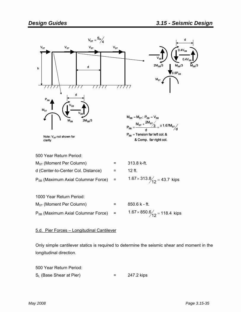
May 2008 Page 3.15-35
d
col. right far Comp. & & col. left far Tension P
dM67.1
d3
M2MP
VP ;MM
SB
STST
STSB
SBSBSTSB
=
±=+
=
==
VST VST VST
MST
h
MSB 2MSB/3
VSB
VSB
PSB
d
Note: VST not shown for clarity
4SV P
ST =
VST
2MSB/3 MSB/3
0.4VSB
VSB
d
MST
0.6PSB
MSB/3
0.4VSB
d
col. right far Comp. & & col. left far Tension P
dM67.1
d3
M2MP
VP ;MM
SB
STST
STSB
SBSBSTSB
=
±=+
=
==
VST VST VST
MST
h
MSB 2MSB/3
VSB
VSB
PSB
d
Note: VST not shown for clarity
4SV P
ST =
VST
2MSB/3 MSB/3
0.4VSB
VSB
d
MST
0.6PSB
MSB/3
0.4VSB
500 Year Return Period:
MST (Moment Per Column) = 313.8 k-ft.
d (Center-to-Center Col. Distance) = 12 ft.
PSB (Maximum Axial Columnar Force) = kips 7.43128.31367.1 =×
1000 Year Return Period:
MST (Moment Per Column) = 850.6 k - ft.
PSB (Maximum Axial Columnar Force) = kips 4.118126.85067.1 =×
5.d. Pier Forces – Longitudinal Cantilever
Only simple cantilever statics is required to determine the seismic shear and moment in the
longitudinal direction.
500 Year Return Period:
SL (Base Shear at Pier) = 247.2 kips

Design Guides 3.15 - Seismic Design
Page 3.15-36 May 2008
Column Height (Clear) = 12.5 ft.
Cap Beam Height = 4.0 ft.
VSL (Shear Per Column) = kips 8.6142.247 =
MColBot(SLB) (Moment Per Column) = ( ) ft.-k 7.101945.128.61 =+×
1000 Year Return Period:
SL (Base Shear at Pier) = 540.7 kips
VSL (Shear Per Column) = kips 2.13547.540 =
MColBot(SLB) (Moment Per Column) = ( ) ft.-k 8.223045.122.135 =+×
6. Seismic Design Forces for Multiple Column Bent Including R-Factor, P-Δ, and
Combination of Orthogonal Forces – 500 and 1000 Year Design Earthquake Return
Period
6.a. R-Factor
R-Factors should only be used to reduce the moments calculated from the base shears of
an “elastic” analysis as was conducted above. As recommended in the Bridge Manual
(Section 3.15.4.4.3) and the LRFD Code for “Essential Bridges” an R-Factor of 3.5 will be
used for the bent in this example. LFD Div. I-A recommends a value of 5 for this bent type.
The R-Factor tables in LRFD and LFD have some differences which have the potential to
cause confusion. There have also been questions over the years about how the described
bridge types in the R-Factor tables in both LRFD and LFD “fit” with actual Illinois bridges in
practice. Section 3.15.4.4 of the Bridge Manual attempts to answer some of these
questions by providing specific recommendations for R-Factors for a number of common
pier types built in Illinois.
6.b. P-Δ
Exacting methods for determining amplification of bending moments for P-Δ effects is not
considered overly significant by the Department in most cases for seismic design of bridges.
For bents of the type in this example, which have a relatively short clear column height (10
Design Guides 3.15 - Seismic Design
May 2008 Page 3.15-37
to 15 ft.), the amplification can be estimated as 5% for both the transverse and longitudinal
directions. In the range of 15 to 20 ft., the amplification may be estimated as 10%. For
greater heights, P-Δ effects may either be calculated or estimated by adding 5% for each 5
ft. increment above 20 ft. clear height. The estimates given above also apply to multiple
column drilled shaft bents with crashwall.
Columns in individually encased piles bents and individual drilled shaft bents tend to have
longer “effective clear heights” extending from the bottom of the cap to the depth-of-fixity.
The methods given above for estimating P-Δ effects for these bent types are permitted at
the discretion of the designer.
P-Δ effects should not be considered for walls, hammerheads, modified hammerheads, solid
wall encased pile bents, solid wall encased drilled shaft bents, and piles analyzed and
designed as columns.
6.c. Summary and Combination of Orthogonal Column Forces Used for Design
The forces on the two exterior columns in the example bridge are focused on for design
because they experience the most extreme earthquake forces. The pier columns should be
designed for the possibility of earthquake accelerations which can be in opposite transverse
directions and opposite longitudinal directions. They are also required to be designed for
the cases “mostly longitudinal and some transverse accelerations” (Longitudinal Dominant –
Load Case 1) and “some longitudinal and mostly transverse accelerations” (Transverse
Dominant – Load Case 2).
Since the bridge in this example has round columns and is not skewed, the summary and
combination of orthogonal forces used for design is straightforward. More complex cases
with skew and non-round columns are considered in subsequent examples in this design
guide. The equations below present the basic method for combination of orthogonal forces.
Load Case 1 (Longitudinal Dominant) Load Case 2 (Transverse Dominant)
Tz
Lz
Dz V3.0V0.1V += T
zLz
Dz V0.1V3.0V +=
Design Guides 3.15 - Seismic Design
Page 3.15-38 May 2008
Ty
Ly
Dy V3.0V0.1V += T
yLy
Dy V0.1V3.0V +=
Tz
Lz
Dz M3.0M0.1M += T
zLz
Dz M0.1M3.0M +=
Ty
Ly
Dy M3.0M0.1M += T
yLy
Dy M0.1M3.0M +=
TLD P3.0P0.1P += TLD P0.1P3.0P +=
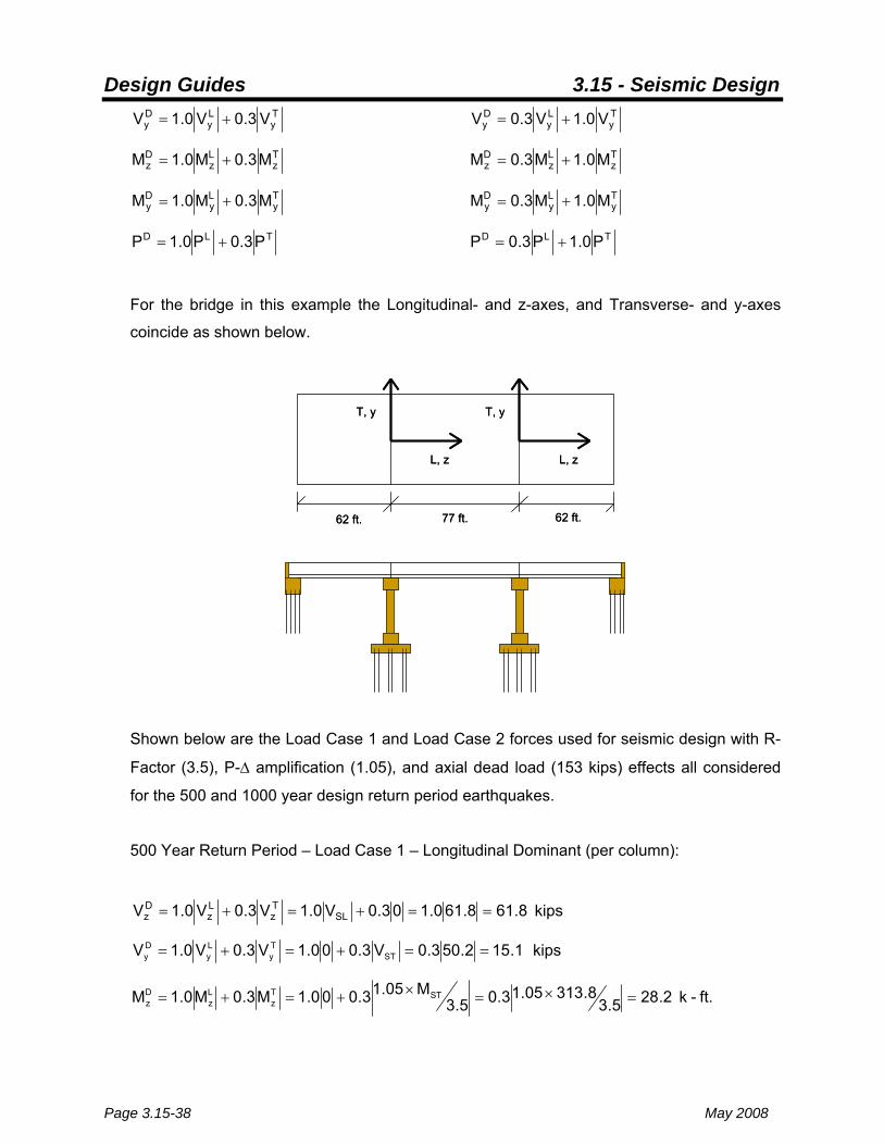
For the bridge in this example the Longitudinal- and z-axes, and Transverse- and y-axes
coincide as shown below.
62 ft. 77 ft. 62 ft.
L, z
T, y
L, z
T, y
62 ft. 77 ft. 62 ft.
L, z
T, y
L, z
T, y
Shown below are the Load Case 1 and Load Case 2 forces used for seismic design with R-
Factor (3.5), P-Δ amplification (1.05), and axial dead load (153 kips) effects all considered
for the 500 and 1000 year design return period earthquakes.
500 Year Return Period – Load Case 1 – Longitudinal Dominant (per column):
kips 8.618.610.103.0V0.1V3.0V0.1V SLTz
Lz
Dz ==+=+=
kips 1.152.503.0V3.000.1V3.0V0.1V STTy
Ly
Dy ==+=+=
ft.-k 2.285.38.31305.13.05.3
M05.13.000.1M3.0M0.1M STTz
Lz
Dz =×=×+=+=

Design Guides 3.15 - Seismic Design
May 2008 Page 3.15-39
ft.-k 9.3055.37.101905.10.103.05.3
M05.10.1M3.0M0.1M SLBTy
Ly
Dy =×=+×=+=
kips 9.177 and 1.128
7.432.393.0153PP3.000.1PPP3.0P0.1P SBSTDeadDTLD
=
=+±=+±+=→+=
Note that the Department recommends a load factor of 1.0 be used for dead loads for LRFD
and LFD design.
The design shears and moments can be added (as vectors) since the columns are round in
order to further simplify the design forces.
kips 6.631.158.61V 22D =+=
ft.-k 2.3079.3052.28M 22D =+=
kips 177.9 and 1.128PD =
500 Year Return Period – Load Case 2 – Transverse Dominant (per column):
kips 5.188.613.000.1V3.0V0.1V3.0V SLTz
Lz
Dz ==+=+=
kips 50.22.500.1V0.103.0V0.1V3.0V STTy
Ly
Dy ==+=+=
ft.-k 1.945.38.31305.10.15.3
M05.10.103.0M0.1M3.0M STTz
Lz
Dz =×=×+=+=
ft.-k 8.915.37.101905.13.000.15.3
M05.13.0M0.1M3.0M SLBTy
Ly
Dy =×=+×=+=
kips 235.9 and 1.70
7.432.390.1153PP0.103.0PPP0.1P3.0P SBSTDeadDTLD
=
=+±=+±+=→+=
Further simplification of the design shears and moments leads to the following.
kips 5.532.505.18V 22D =+=
ft.-k 5.1318.911.94M 22D =+=
kips 235.9 and 1.70PD =
Design Guides 3.15 - Seismic Design
Page 3.15-40 May 2008
1000 Year Return Period – Load Case 1 – Longitudinal Dominant (per column):
The same form of the calculations above leads to the following simplified design forces.
kips 2.1418.402.135V 22D =+=
ft.-k 6.6736.762.669M 22D =+=
kips 220.4 and 6.85PD =
1000 Year Return Period – Load Case 2 – Transverse Dominant (per column):
The same form of the calculations above leads to the following simplified design forces.
kips 0.1421.1366.40V 22D =+=
ft.-k 7.3242.2558.200M 22D =+=
kips 377.7 and 7.71PD −= (Negative indicates tension)
7. Column Design Including Overstrength Plastic Moment Capacity – 500 and 1000
Year Design Earthquake Return Period
7.a. Column Design for Axial Force and Moment
Since the columns in the example pier bents are round, a simple uni-axial bending – axial
force interaction diagram formulation can be used for design and compared with the forces
calculated above. For the 500 year earthquake return period, the example bridge is in
Category B. As such, the φ factor (strength reduction factor) used for design should be 0.75.
For the 1000 year earthquake return period, the example bridge is located in Zone 3 and the
φ factor is 1.0 according to the recommendation in Section 3.15.4.4.1 of the Bridge Manual.

Design Guides 3.15 - Seismic Design
May 2008 Page 3.15-41
500 Year Return Period Column Design:
In order to compare the design axial forces and moments calculated above to a “nominal” or
unreduced column interaction diagram, they should be divided by the φ factor (0.75). These
computations are shown below.
Load Case 1 – Longitudinal Dominant Load Case 2 – Transverse Dominant
ft.-k 6.40975.02.307MD
==φ ft.-k 3.17575.05.131MD
==φ
kips 170.8 75.01.128PD
==φ kips 93.5 75.01.70PD
==φ
kips 237.2 75.09.177PD
==φ kips 314.5 75.09.235PD
==φ
For design of the columns, try:
10 - #9 bars (Gr. 60 A706 Bars) with #5 Spiral and a Clear Cover of 2 in. The center-to-
center spacing of the vertical steel is about 7 ½ in. which is less than the suggested 8 in.
maximum. The percentage of steel in relation to the gross area of the column is about 1.4%
which is well within the realm of reasonable for this bridge and the accelerations associated
with the 500 year design earthquake.
The column interaction diagram is shown below. The load cases calculated above are
superimposed on the diagram along with the load cases for the middle columns.

Design Guides 3.15 - Seismic Design
Page 3.15-42 May 2008
1000 Year Return Period Column Design:
Since the φ factor is one for this case, the design axial forces and moments calculated
above do not need to be transformed in order compare them to a “nominal” or unreduced
column interaction diagram. The forces from Load Cases 1 and 2 are repeated below.
Load Case 1 – Longitudinal Dominant Load Case 2 – Transverse Dominant
ft.-k 6.673MD = ft.-k 7.324MD =
kips 6.85PD = kips 7.71PD −=
kips 220.4PD = kips 377.7PD =
For design of the columns, try:
10 - #10 bars (Gr. 60 A706 Bars) with #5 Spiral and a Clear Cover of 2 in. The center-to-
center spacing of the vertical steel is about 7 ½ in. which is less than the suggested 8 in.
maximum. The percentage of steel in relation to the gross area of the column is about 1.8%

Design Guides 3.15 - Seismic Design
May 2008 Page 3.15-43
which is well within the realm of reasonable for this bridge and the accelerations associated
with the 1000 year design earthquake.
The column interaction diagram is shown below. The load cases calculated above are
superimposed on the diagram along with the load cases for the middle columns.
7.b. Column Design for Shear
For multiple column bents, the Department prefers that spirals and ties have a constant
spacing for the full length of the column and required extensions into the cap beam and
crashwalls. Various detailing options for shear reinforcement are permitted and described in
Section 3.15.5 of the Bridge Manual. Specific details are not covered in this forum. Rather,
methods for determining the required bar sizes and spacing for shear reinforcement which
satisfy the LRFD and LFD Specifications are focused on.
The design requirements for shear are similar for Category B (LFD) and Zone 3 (LRFD). A
minimum amount of steel is required in plastic hinging regions for “confinement” to ensure
flexural capacity integrity during an earthquake and the spirals or ties shall also satisfy
strength requirements. In Category B, the elastic shear (calculated above for this example)
should be used for design. For Zone 3, however, the lesser of the elastic shear or the shear

Design Guides 3.15 - Seismic Design
Page 3.15-44 May 2008
which causes plastic hinging in the columns may be used for design. The shear which
causes plastic hinging can be determined from a simple axial-flexural “overstrength”
capacity analysis. As recommended in Section 3.15.5.1 of the Bridge Manual, it is simplest
to assume that the concrete strength is zero (Vc = 0.0) when designing columnar shear
reinforcement without verifying whether some nominal value for Vc is allowed to be
considered by LRFD or LFD. Typically, at least the outer columns in multiple column bents
either have a low compressive design force or are in tension. When columns are in tension,
the shear strength of the concrete should be taken as zero according to LRFD and LFD.
The following are equations which should be used for the design of spirals in round columns
with Vc = 0.
Minimum steel required for confinement expressed as a volumetric ratio:
yh
'c
c
gs f
f1
AA
45.0 ⎟⎟⎠
⎞⎜⎜⎝
⎛−≥ρ (LRFD Eq. 5.7.4.6-1, LFD Div. I-A Eq. 6-4 and 7-4)
And,
yh
'c
s ff
12.0≥ρ (LRFD Eq. 5.10.11.4.1d-1, LFD Div. I-A Eq. 6-5 and 7-5)
Where:
Ag = gross area of concrete section (in.2)
Ac = area of core measured to the outside diameter of the spiral (in.2) 'cf = compressive strength of concrete (ksi)
fyh = yield strength of spiral reinforcement (ksi)
Strength of provided steel:
sdfA
V vyhvs φ=φ (LRFD Eq. 5.8.3.3-4, LFD Eq. 8-53)

Design Guides 3.15 - Seismic Design
May 2008 Page 3.15-45
Where:
Av = area of shear reinforcement within a distance s (in.2)
dv = effective shear depth (in.)
s = spacing of spiral (in.)
φ = 0.9 for LRFD and 0.85 for LFD (however, use 0.9 for LFD)
The equation above for LRFD has been simplified according to the provisions in Article
5.8.3.4.1.
The equations for minimum required confinement steel for tied rectangular or trapezoidal
columns are similar to those for round columns and found in the same referenced sections
above. When cross ties are used, which is common, they are counted in the total
reinforcement area resisting the design shear. The shear requirements for wall type piers
are somewhat different than for columns. However, they are not complex. If a wall is
designed as a column in its weak direction, the shear design method is the same as that for
a column. If a wall is not designed as column in its weak direction, it shall be designed for
shear in the same manner as for the strong direction. The minimum reinforcement ratios
and shear strength design equations for walls (in the strong and possibly the weak direction)
are given in LRFD 5.10.11.4.2 and LFD Div. I-A 7.6.3. The provisions in both specifications
are comparable.
The shear design calculations for the 500 and 1000 year design return period earthquakes
for the Example 1 bridge are given below using the elastic design forces. The method for
calculating the plastic design shear using “overstrength” is demonstrated afterward for the
1000 year earthquake case. Note, however, that for many typical bridges in Illinois, even
those in Zones 3 and 4, the shear requirements might easily be met by using the elastic
design shears.
500 Year Return Period Shear Design:
Minimum steel required,
0087.060
5.31131545.0
ff
1AA
45.0 2
2
yh
'c
c
gs =⎟⎟
⎠
⎞⎜⎜⎝
⎛−
×π×π
=⎟⎟⎠
⎞⎜⎜⎝
⎛−≥ρ

Design Guides 3.15 - Seismic Design
Page 3.15-46 May 2008
And,
0070.060
5.312.0ff
12.0yh
'c
s ==≥ρ
Try #5 spirals at a spacing of 4 in. center-to-center,
( ) OK 0087.00119.042230
31.04sD
2A4
turn spiral 1 in concrete of Volumeturn spiral 1 of Volume
core
v
s >=×−−
×=
×
⎟⎠⎞⎜
⎝⎛
==ρ
Dcore is the diameter of the column out-to-out of the spiral and Av is the area of 2 bars.
kips 7.1694
27.206031.029.0s
dfAV vyhv
s =×××
=φ=φ
The effective depth, dv, may be calculated with the method suggested below in the
commentary of the LRFD Specifications.
dv = in. 27.2062.232
309.0D
2D9.0d9.0 r
e =⎟⎠⎞
⎜⎝⎛
π+=⎟
⎠
⎞⎜⎝
⎛π
+= (LRFD C5.8.2.9)
Where:
D = gross diameter of column (in.)
Dr = diameter of the circle passing through the centers of longitudinal
reinforcement (in.)
Comparing the elastic design shear forces for Load Case 1 and Load Case 2 gives:
Load Case 1: 63.6 < 169.7 OK
Load Case 2: 53.5 < 169.7 OK

Design Guides 3.15 - Seismic Design
May 2008 Page 3.15-47
∴#5 spiral at 4 in. center-to-center spacing OK (and the comparisons above indicate that a
spacing as large as 6 in. center-to-center may also be acceptable).
1000 Year Return Period Shear Design:
Minimum steel required,
0087.0ff
1AA
45.0yh
'c
c
gs =⎟⎟
⎠
⎞⎜⎜⎝
⎛−≥ρ and 0070.0
ff
12.0yh
'c
s =≥ρ
Try #5 spirals at a spacing of 4 in. center-to-center,
OK 0087.00119.0sD
2A4
core
v
s >=×
⎟⎠⎞⎜
⎝⎛
=ρ
kips 3.1694
23.206031.029.0s
dfAV vyhv
s =×××
=φ=φ
dv = in. 23.2048.232
309.0D
2D9.0d9.0 r
e =⎟⎠⎞
⎜⎝⎛
π+=⎟
⎠
⎞⎜⎝
⎛π
+= (LRFD C5.8.2.9)
Comparing the elastic design shear forces for Load Case 1 and Load Case 2 gives:
Load Case 1: 141.2 < 169.3 OK
Load Case 2: 142.0 < 169.3 OK
∴#5 spiral at 4 in. center-to-center spacing OK.
7.c. 1000 Year Return Period Plastic Shear Determination Using Overstrength
In Illinois, the determination of plastic shear capacity using overstrength should generally be
confined to bridge types for which the plastic hinges in the substructure elements would
form above ground at the piers during the design earthquake. This typically entails bents
with cap beams, crashwalls and multiple columns which are either circular or trapezoidal.

Design Guides 3.15 - Seismic Design
Page 3.15-48 May 2008
However, the Department does not discourage overstrength analysis for such pier types as
individual column drilled shaft bents or drilled shaft bents with web walls.
Once the columns have been designed to resist axial forces and moments in a ductile
manner (with an R-Factor), the other components of the bridge can be designed for the
lesser of the base shear which actually causes the columns to form plastic hinges or the
elastic forces from the original analysis. The “overstrength” of a column can be thought of
as a simplified engineering estimate of the base shear required to cause plastic hinging. For
typical cases in Illinois, these components are usually only the columnar shear
reinforcement and the piles.
Overstrength analysis is reserved for bridges located in regions where design accelerations
are considered significant. For the 500 year design return period earthquake, this translates
to LFD Seismic Performance Categories C and D and for the 1000 year seismic event it
corresponds to LRFD Seismic Performance Zones 3 and 4 (and 2, but not explicitly).
The overstrength column capacity should be calculated by one of two methods depending
on the levels of axial forces used to design the vertical steel in a column. When the design
axial forces generally fall below the balanced failure point on the nominal column axial force-
moment interaction diagram, the overstrength of a concrete column should be determined
by only multiplying the moment strength by 1.3. If the design axial forces generally fall
above the balanced failure point, the nominal axial and moment strengths should both be
multiplied by 1.3. Once the overstrength curve has been calculated, a simple procedure is
used to determine the plastic shear capacities for the longitudinal and transverse directions.
This procedure is outlined in LRFD Article 3.10.9.4.3 and LFD Div. I-A Article 7.2.2 for piers
with either single or multiple columns. A plot of the overstrength capacity for the pier
columns of the Example 1 bridge is shown below for the 1000 year design earthquake.

Design Guides 3.15 - Seismic Design
May 2008 Page 3.15-49
Since the axial design forces fall below the balance point, only the nominal moment
strengths were multiplied by 1.3. The calculations and descriptions below detail the method
for determining the plastic shear capacities for the transverse and longitudinal directions of
the Example 1 bridge.
Initial Plastic Moment Capacity:
For multiple column bents, the initial design axial force used to determine the initial
corresponding plastic moment capacity should be that from the dead load only. Referring to
the overstrength axial force-moment interaction diagram above,
Initial Axial Dead Load = 153 kips
Initial Plastic Moment = 944 kip-ft.

Design Guides 3.15 - Seismic Design
Page 3.15-50 May 2008
Initial Plastic Shear Capacity:
The plastic shear capacities for the transverse and longitudinal directions are found with the
same basic statics equations used above for determining elastic column moments. The
unknowns to solve for, though, are shears instead of moments.
Long. Shear
( )
kips 8.2282.574 Vand
nkips/colum 2.575.16944V
ft. 4 ft. 5.12Vft.-kip 944M
Bent Long.Plastic
Long.Plastic
Long.Plastic P
=×=
==∴
+×==
Trans. Shear
kips 0.6041514 Vand
nkips/colum 0.1515.122944V
2ft. 5.12Vft.-kip 944M
Bent Trans.Plastic
.nsPlasticTra
Trans.Plastic P
=×=
=×=∴
⎟⎠⎞
⎜⎝⎛×==
Initial Overturning and Frame Action Axial Forces from Initial Plastic Base Shears:
Longitudinal There are no overturning or frame action axial forces from base shears
applied in the longitudinal direction. Consequently, the initial longitudinal
plastic shear calculated above is the final plastic shear.
Transverse Using methods from the elastic analyses above.
Overturning:
Sp (Base Shear at Pier) = 604.0 kips
M (Overturning Moment) = ft.-k 8.47188125.7604 =×
PST (Max. Axial Col. Force) = kips 0.118128.4718
103
=
Frame Action:
Sp (Base Shear at Pier) = 604.0 kips
VST (Shear Per Column) = kips 0.15140.604 =

Design Guides 3.15 - Seismic Design
May 2008 Page 3.15-51
MST (Moment Per Column) = ft.-k 8.94325.120.151 =×
PSB (Max. Axial Col. Force) = kips 3.131128.94367.1 =×
Total “Plastic” Axial Force:
PDPlastic = 153.0 + 118.0 + 131.3 = 402.3 kips
Revised Overstrength Moment Resistance:
Long. Not required (see above).
Trans. Taking PDPlastic (402.3 kips) as the design axial force (instead of just the
dead load) and referring again to the overstrength axial force-moment
interaction diagram above, a plastic moment of 1082 kip-ft. is obtained.
The corresponding plastic shear per column is 173.1 kips and for the bent
the plastic shear is about 692.4 kips. This plastic base shear is within
about 15% of the first base shear value (604.0 kips). According to the
method, a further iteration should be performed such that successive
values of calculated plastic base shears are within 10% of each other.
The next iteration would start at the “Overturning and Frame Action Axial
Forces from Plastic Base Shears” step with a base shear of 692.4 kips.
However, another iteration is not necessary because the calculated
plastic base shear has already been shown to be greater than the design
elastic shear (544.2 kips). As such, the elastic force may be used for
design.
Overstrength Summary:
Longitudinal Elastic Base Shear = 540.7 kips
Plastic Base Shear = 228.8 kips
Transverse Elastic Base Shear = 544.2 kips
Plastic Base Shear = ≈ 692 kips
Design Guides 3.15 - Seismic Design
Page 3.15-52 May 2008
According to the provisions of LFD Div. I-A, it can be interpreted as acceptable to use the
plastic longitudinal base shear in conjunction with the elastic transverse base shear for the
design of the columnar shear reinforcement and the piles for the Example 1 bridge. This
may not be the case for LRFD, though. LRFD appears to steer the engineer towards
“consistently” using either the elastic or plastic cases. Either the LFD or apparent LRFD
approach, however, is permitted by the Department (regardless of which code the bridge is
being designed under) and left to the designer’s judgment.
The results of the overstrength analysis and their potential impact on the design of the
Example 1 bridge are somewhat typical for multiple column bents in Illinois. As shown
above, the benefits of overstrength analysis were not required to design the columnar shear
reinforcement with a reasonable spiral size and spacing for the 1000 yr. seismic event. As
such, the use of overstrength analysis should be carefully considered by the designer. For
many cases in Illinois, it is more straightforward and simpler to use the elastic design forces
calculated from the initial determination of the bridge periods.
8. Pile Design Overview
Seismic design forces for the piles at piers and abutments in the Example 1 bridge can be
determined with methods which are analogous to those described above for the pier columns in
the transverse direction. Each row of piles at the piers along the transverse and longitudinal
directions can be treated as an individual frame in the soil as if it were a column bent. For
example, consider the case where the pier foundations for the Example 1 Bridge has two rows
of ten piles. In the transverse direction, there would be two pile bent frames with 9 “portals”,
each analyzed as taking half the transverse base shear at a pier. In the longitudinal direction,
there would be ten single portal frames with each analyzed as taking one-tenth of the
longitudinal base shear. The overturning “moment arm” is longer for the piles and should
extend down to the bottom of the footing. Note that there is overturning moment for both the
transverse and longitudinal directions. In the longitudinal direction, the analysis is not for a
cantilever as it is for the columns. It is most straightforward to use the elastic base shears in the
transverse and longitudinal directions in which the design moments are unreduced (R = 1.0).
For many cases, the pile fixity depths for steel H-piles provided in Appendix C (which are
presented in terms of “moment fixity” and not “deflection fixity”) can be used for design.

Design Guides 3.15 - Seismic Design
May 2008 Page 3.15-53
Guidance on the appropriateness of their use is also provided in Appendix C. Overturning
analysis solutions for cases with up to 13 columns or piles in a frame are provided in Appendix
A. Frame analysis solutions for any number of portals are provided in Appendix B. Example 4
may also be referenced for additional guidance concerning simple structural analysis techniques
for piles in global and local models. More complex or sophisticated analysis methods are not
discouraged by the Department and may be appropriate depending on the bridge being
designed.
“Group Action” for piles may be considered by the designer, but this is not required when using
the methods presented in the examples and appendices of this design guide for regular or
typical bridges.
Structurally, the piles should be designed for shear, and combined axial force (including
compression and tension as appropriate) and bending. Piles can be assumed to be continually
braced throughout their length in the soil. Pullout of the piles from the footing is also a
consideration. When required, special seismic pile anchorage details in footings should be used
and are provided in Section 3.15.5.5 of the Bridge Manual. Reference Parts 8 and 9 of Example
4 for example calculations that check the structural capacity of steel H-piles.
The piles in the Example 1 bridge could also be metal shell. Metal shell piles should be
designed structurally for shear, and combined axial force and moment just as H-piles are. Metal
shell piles behave as reinforced concrete columns in soil with the shell acting as the
reinforcement. Supplemental longitudinal (vertical) and shear/confinement (spiral)
reinforcement may also be provided inside of metal shell piles to increase structural capacity.
Appendix C provides fixity depths, and nominal axial force–moment strength interaction
diagrams for metal shell piles without supplemental reinforcement. See Section 3.15.5.5 of the
Bridge Manual and Part 14 of Example 4 for additional guidance.
Geotechnical considerations for the design of piles to resist seismic loadings are provided in
Sections 3.10 and 3.15 of the Bridge Manual as well as Design Guide 3.10.1. Guidance on
liquefaction, lateral pile resistance in soil, pullout from the soil, etc. are among the
considerations addressed.

Design Guides 3.15 - Seismic Design
Page 3.15-54 May 2008
Example 2 Example 1 Bridge with a Skew of 30° for the 500 Year Design Earthquake Return Period
The primary focus of this example is to examine the differences from Example 1 in how pier
column seismic design forces are calculated when a bridge is skewed. The methods described
in Example 2 are also applicable to pile seismic design force calculations for this and other
similar bridge types which are skewed. The secondary focus of Example 2 is the effects of
skew on the determination of bridge periods and base shears in the transverse and longitudinal
directions.
42 ft.
6 spaces @ 6 ft. = 36 ft.
7 ½ in. 1 ½ in. Added Surface13
42 ft.
6 spaces @ 6 ft. = 36 ft.
7 ½ in. 1 ½ in. Added Surface13
E F E EE F E E
62 ft. 77 ft. 62 ft.62 ft. 77 ft. 62 ft.
12 ft. –6 in. 2 ft. – 6 in.
4 ft.
4 ft.2 ft. – 3 in.
12 ft. –6 in. 2 ft. – 6 in.
48 ft. -6 in.
4 ft.
4 ft.2 ft. – 3 in.
14 ft.
42 ft.
6 spaces @ 6 ft. = 36 ft.
7 ½ in. 1 ½ in. Added Surface13
42 ft.
6 spaces @ 6 ft. = 36 ft.
7 ½ in. 1 ½ in. Added Surface13
E F E EE F E EE F E EE F E E
62 ft. 77 ft. 62 ft.62 ft. 77 ft. 62 ft.62 ft. 77 ft. 62 ft.62 ft. 77 ft. 62 ft.
12 ft. –6 in. 2 ft. – 6 in.
4 ft.
4 ft.2 ft. – 3 in.
12 ft. –6 in. 2 ft. – 6 in.
48 ft. -6 in.
4 ft.
4 ft.2 ft. – 3 in.
14 ft.12 ft. –6 in. 2 ft. – 6 in.
4 ft.
4 ft.2 ft. – 3 in.
12 ft. –6 in. 2 ft. – 6 in.
48 ft. -6 in.
4 ft.
4 ft.2 ft. – 3 in.
14 ft.
1. Determination of Bridge Periods and Base Shears – 500 Year Design Earthquake
Return Period
For Example 2, assume that the weight of the bridge used for seismic/dynamic analysis
calculations is the same as that for Example 1 (there is only a nominal increase in weight due to
the increased length of the cap beams). Further assume that the stiffness of the abutments is
the same as that for the bridge in Example 1 even though the piles are at a 30° skew. In reality,
the abutment stiffnesses are comparable to those for the Example 1 case (See methods of
Example 3 Part 2 and in Appendix C). Consequently, this assumption does not introduce a
significant “error” in the dynamic analysis of the structure. The “global” transverse and
longitudinal axes of the bridge are shown below along with the “local” pier axes.
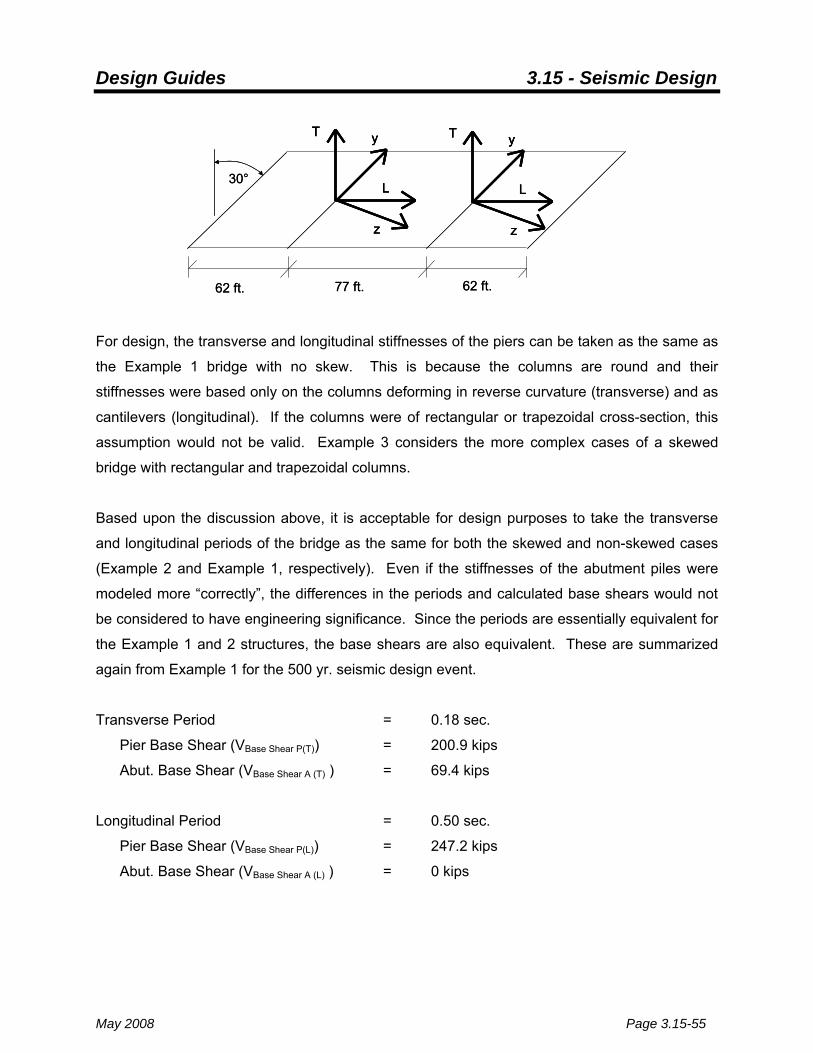
Design Guides 3.15 - Seismic Design
May 2008 Page 3.15-55
62 ft. 77 ft. 62 ft.
L
yT
z
L
yT
z
30°
62 ft. 77 ft. 62 ft.
L
yT
z
L
yT
z
L
yT
z
L
yT
z
30°
For design, the transverse and longitudinal stiffnesses of the piers can be taken as the same as
the Example 1 bridge with no skew. This is because the columns are round and their
stiffnesses were based only on the columns deforming in reverse curvature (transverse) and as
cantilevers (longitudinal). If the columns were of rectangular or trapezoidal cross-section, this
assumption would not be valid. Example 3 considers the more complex cases of a skewed
bridge with rectangular and trapezoidal columns.
Based upon the discussion above, it is acceptable for design purposes to take the transverse
and longitudinal periods of the bridge as the same for both the skewed and non-skewed cases
(Example 2 and Example 1, respectively). Even if the stiffnesses of the abutment piles were
modeled more “correctly”, the differences in the periods and calculated base shears would not
be considered to have engineering significance. Since the periods are essentially equivalent for
the Example 1 and 2 structures, the base shears are also equivalent. These are summarized
again from Example 1 for the 500 yr. seismic design event.
Transverse Period = 0.18 sec.
Pier Base Shear (VBase Shear P(T)) = 200.9 kips
Abut. Base Shear (VBase Shear A (T) ) = 69.4 kips
Longitudinal Period = 0.50 sec.
Pier Base Shear (VBase Shear P(L)) = 247.2 kips
Abut. Base Shear (VBase Shear A (L) ) = 0 kips

Design Guides 3.15 - Seismic Design
Page 3.15-56 May 2008
2. Frame Analysis and Columnar Seismic Forces for Multiple Column Bent – 500 Year
Design Earthquake Return Period
When a bridge is skewed, the global transverse and longitudinal pier and abutment axes do not
coincide with the local axes as shown above. As such, a separate local transverse (y-axis) and
longitudinal (z-axis) axis force analysis is required for both the global transverse (T-axis) and
longitudinal (L-axis) axes. These analyses are presented below for the exterior columns. Note
that the subscripts and superscripts for the axial forces, shears, and moments presented below
are different from Example 1 for this more complex case. They “match” the variables used
when the forces are combined orthogonally in Section 3 of this example.
2.a Pier Forces – Dead Load
Design Dead Load Per Column = 153.0 kips (from Example 1)
2.b. Pier Forces from Global Transverse Base Shear
The component of the global transverse (T-axis) base shear in the local transverse (y-axis)
direction produces axial forces in the columns from overturning and frame action as well as
moments from the columns deforming in reverse curvature. The component of the global
transverse base shear in the local longitudinal (z-axis) produces a cantilever moment. The
components of the global transverse base shear in the local y- and z-directions are given
below.
VT(Bent) = VBase Shear P(T) = 200.9 kips )Bent(T
yV = VT cos 30° = 200.9 cos 30° = 174.0 kips
)Bent(TzV = VT sin 30° = 200.9 sin 30° = 100.5 kips
The forces from overturning (moments about local z-axis, forces in local y-axis direction)
are,

Design Guides 3.15 - Seismic Design
May 2008 Page 3.15-57
Sp
d d
PSTarm0.33PST
d
PST
0.33PST
( )( )
dM
103P
dP2 dP2M
armSM
ST
21
ST31
23
ST
p
=∴
×
+×=
×=
Sp
d d
PSTarm0.33PST
d
PST
0.33PST
( )( )
dM
103P
dP2 dP2M
armSM
ST
21
ST31
23
ST
p
=∴
×
+×=
×=
)Bent(TyV = Sp = 174.0 kips
arm = 7.8125 ft. (Example 1)
d = 14 ft.
M (Overturning Moment) = ft.-k 4.13598125.70.174 =×
TSP = PST = kips 1.2914
4.1359103
=
The forces from frame action (moments about local z-axis, forces in local y-axis direction)
are,
d d 2hVM ST
ST×=
VST VST VST
VST
VST
MST
MST
h
4SV P
ST =
d
VST
d d 2hVM ST
ST×=
VST VST VST
VST
VST
MST
MST
h
4SV P
ST =
d
VST

Design Guides 3.15 - Seismic Design
Page 3.15-58 May 2008
)Bent(T
yV = Sp = 174.0 kips
Column Height (Clear) = 12.5 ft. TyV = VST = kips 5.434
0.174 =
TzM = MST = ft.-k 9.2712
5.125.43 =×
d
col. right far Comp. & & col. left far Tension P
dM67.1
d3
M2MP
VP ;MM
SB
STST
STSB
SBSBSTSB
=
±=+
=
==
VST VST VST
MST
h
MSB 2MSB/3
VSB
VSB
PSB
d
Note: VST not shown for clarity
4SV P
ST =
VST
2MSB/3 MSB/3
0.4VSB
VSB
d
MST
0.6PSB
MSB/3
0.4VSB
d
col. right far Comp. & & col. left far Tension P
dM67.1
d3
M2MP
VP ;MM
SB
STST
STSB
SBSBSTSB
=
±=+
=
==
VST VST VST
MST
h
MSB 2MSB/3
VSB
VSB
PSB
d
Note: VST not shown for clarity
4SV P
ST =
VST
2MSB/3 MSB/3
0.4VSB
VSB
d
MST
0.6PSB
MSB/3
0.4VSB
TzM = MST = 271.9 k-ft.
d = 14 ft. TBP = PSB = kips 32.4 14
9.27167.1 =×
The moments about the local y-axis, and forces in the local z-axis direction are,
SL = 100.5 kips
Column Height (Clear) = 12.5 ft.
Cap Beam Height = 4.0 ft. TzV = VSL = kips 1.254
5.100 =

Design Guides 3.15 - Seismic Design
May 2008 Page 3.15-59
TyM = MColBot(SLB) = ( ) ft.-k 2.41445.121.25 =+×
2.c. Pier Forces from Global Longitudinal Base Shear
The component of the global longitudinal (L-axis) base shear in the local transverse (y-axis)
direction produces axial forces in the columns from overturning and frame action as well as
moments from the columns deforming in reverse curvature. The component of the global
longitudinal base shear in the local longitudinal (z-axis) produces a cantilever moment. The
components of the global longitudinal base shear in the local y- and z-directions are given
below.
VL(Bent) = VBase Shear P(T) = 247.2 kips )Bent(L
yV = VL sin 30° = 247.2 sin 30° = 123.6 kips
)Bent(LzV = VL cos 30° = 247.2 cos 30° = 214.1 kips
The forces from overturning (moments about local z-axis, forces in local y-axis direction)
are,
Sp
d d
PSTarm0.33PST
d
PST
0.33PST
( )( )
dM
103P
dP2 dP2M
armSM
ST
21
ST31
23
ST
p
=∴
×
+×=
×=
Sp
d d
PSTarm0.33PST
d
PST
0.33PST
( )( )
dM
103P
dP2 dP2M
armSM
ST
21
ST31
23
ST
p
=∴
×
+×=
×=

Design Guides 3.15 - Seismic Design
Page 3.15-60 May 2008
)Bent(LyV = Sp = 123.6 kips
arm = 7.8125 ft. (Example 1)
d = 14 ft.
M (Overturning Moment) = ft.-k 6.9658125.76.123 =×
LSP = PST = kips 7.2014
6.965103
=
The forces from frame action (moments about local z-axis, forces in local y-axis direction)
are,
d d 2hVM ST
ST×=
VST VST VST
VST
VST
MST
MST
h
4SV P
ST =
d
VST
d d 2hVM ST
ST×=
VST VST VST
VST
VST
MST
MST
h
4SV P
ST =
d
VST
)Bent(L
yV = Sp = 123.6 kips
Column Height (Clear) = 12.5 ft. LyV = VST = kips 9.304
6.123 =
LzM = MST = ft.-k 1.1932
5.129.30 =×

Design Guides 3.15 - Seismic Design
May 2008 Page 3.15-61
d
col. right far Comp. & & col. left far Tension P
dM67.1
d3
M2MP
VP ;MM
SB
STST
STSB
SBSBSTSB
=
±=+
=
==
VST VST VST
MST
h
MSB 2MSB/3
VSB
VSB
PSB
d
Note: VST not shown for clarity
4SV P
ST =
VST
2MSB/3 MSB/3
0.4VSB
VSB
d
MST
0.6PSB
MSB/3
0.4VSB
d
col. right far Comp. & & col. left far Tension P
dM67.1
d3
M2MP
VP ;MM
SB
STST
STSB
SBSBSTSB
=
±=+
=
==
VST VST VST
MST
h
MSB 2MSB/3
VSB
VSB
PSB
d
Note: VST not shown for clarity
4SV P
ST =
VST
2MSB/3 MSB/3
0.4VSB
VSB
d
MST
0.6PSB
MSB/3
0.4VSB
LzM = MST = 193.1 k-ft.
d = 14 ft. LBP = PSB = kips 23.0 14
1.19367.1 =×
The moments about the local y-axis, and forces in the local z-axis direction are,
SL = 214.1 kips
Column Height (Clear) = 12.5 ft.
Cap Beam Height = 4.0 ft. LzV = VSL = kips 5.534
1.214 =
LyM = MColBot(SLB) = ( ) ft.-k 8.88245.125.53 =+×

Design Guides 3.15 - Seismic Design
Page 3.15-62 May 2008
3. Seismic Design Forces for Multiple Column Bent Including R-Factor, P-Δ, and
Combination of Orthogonal Forces – 500 Year Design Earthquake Return Period
3.a. R-Factor
R-Factor = 3.5 (from Example 1)
3.b. P-Δ
P-Δ Amplification = 1.05 (from Example 1)
3.c. Summary and Combination of Orthogonal Column Forces Used for Design
The equations for combination of orthogonal forces are repeated below from Example 1.
Because the bridge is skewed, none of the terms will be equal to zero for Example 2. R-
Factors and P-Δ amplification effects are also included in the calculations.
Load Case 1 (Longitudinal Dominant) Load Case 2 (Transverse Dominant)
Tz
Lz
Dz V3.0V0.1V += T
zLz
Dz V0.1V3.0V +=
Ty
Ly
Dy V3.0V0.1V += T
yLy
Dy V0.1V3.0V +=
Tz
Lz
Dz M3.0M0.1M += T
zLz
Dz M0.1M3.0M +=
Ty
Ly
Dy M3.0M0.1M += T
yLy
Dy M0.1M3.0M +=
TLD P3.0P0.1P += TLD P0.1P3.0P +=
Load Case 1 – Longitudinal Dominant:
kips 0.611.253.05.530.1V3.0V0.1V Tz
Lz
Dz =+=+=
kips 44.0 5.433.09.300.1V3.0V0.1V Ty
Ly
Dy =+=+=
ft.-k 4.825.39.27105.13.05.3
1.19305.10.1M3.0M0.1M Tz
Lz
Dz =×+×=+=

Design Guides 3.15 - Seismic Design
May 2008 Page 3.15-63
ft.-k 1.3025.32.41405.13.05.3
8.88205.10.1M3.0M0.1M Ty
Ly
Dy =×+×=+=
kips 2.215 and 9.90 4.321.293.00.237.200.10.153PP3.0P0.1P DTLD =+±+±=→+=
(Note: Axial Dead Load = 153 kips)
The design shears and moments can be added (as vectors) since the columns are round in
order to further simplify the design forces.
kips 2.750.440.61V 22D =+=
ft.-k 1.3131.3024.82M 22D =+=
kips 215.2 and 9.90PD =
Load Case 2 – Transverse Dominant:
kips 2.411.250.15.533.0V0.1V3.0V Tz
Lz
Dz =+=+=
kips 52.8 5.430.19.303.0V0.1V3.0V Ty
Ly
Dy =+=+=
ft.-k 9.985.39.27105.10.15.3
1.19305.13.0M0.1M3.0M Tz
Lz
Dz =×+×=+=
ft.-k 7.2035.32.41405.10.15.3
8.88205.13.0M0.1M3.0M Ty
Ly
Dy =×+×=+=
kips 6.227 and 4.78 4.321.290.10.237.203.00.153PP0.1P3.0P DTLD =+±+±=→+=
Further simplification of the design shears and moments leads to the following.
kips 0.678.522.41V 22D =+=
ft.-k 4.2267.2039.98M 22D =+=
kips 227.6 and 4.78PD =

Design Guides 3.15 - Seismic Design
Page 3.15-64 May 2008
Example 3 Overview of Bents with Rectangular or Trapezoidal Columns Examples 1 and 2, along with their associated discussions provide a number of techniques and
guidance which can be used for the seismic bridge design of a large number of cases in Illinois
which would be considered typical or common. Example 3 provides an overview of typical
situations in Illinois which have not been covered. These are bridges with rectangular or
trapezoidal columns, especially those on a skew. The provided discussions can also be
extended to the design of bridges with H-piles as appropriate.
1. Overview of Seismic Design of Multiple Column Bents with Rectangular or
Trapezoidal Columns for Bridges with No Skew
For bridges with rectangular or trapezoidal column bents and no skew, there are only a few
differences when designing for seismic loads when compared to designing bridges with round
columns. The rectangular column case is the simplest. The techniques from Example 1 can be
used with one exception being that there are two column moments of inertia to consider. One is
about the longitudinal axis of the bridge (and bent) and the other is about the transverse axis of
the bridge (and bent). However, the major complicating difference from bridges with round
column bents is the design of the columns for axial force and moment. The moments to
consider are bi-axial. At the 500 yr. design level seismic event, more “approximate” methods of
bi-axial column design can be used. At the 1000 yr. seismic event level, though, it is
recommended that more precise design methods be used, although this is not explicitly required
by the Department. It is possible that excessive vertical steel may be called for by not using
more sophisticated bi-axial column design techniques which usually entail the use of
commercial software.
The seismic design of bridges with no skew and trapezoidal columns adds another level of
complexity above that of the consideration of just rectangular columns. Probably the simplest
method for developing a global finite element model of the bridge (for the purposes of period
and base shear calculations) is to determine equivalent rectangular column moments of inertia
for the trapezoidal columns about the transverse and longitudinal axes. The deflections from
equivalent rectangular columns can be equalized to those from simple finite element models of

Design Guides 3.15 - Seismic Design
May 2008 Page 3.15-65
a trapezoidal column about the weak and strong axis to obtain two simple equivalent moments
of inertia for a column such that a value for the stiffness of the bent can be calculated for both
directions. The trapezoidal columns should be “discreetized” into about 5 to 10 finite elements.
Note that a hammerhead pier can be considered as having a single trapezoidal column.
At the local model level, when the vertical steel of trapezoidal columns is being designed, a full
finite element model of the bent with standard frame elements would probably be the analysis
method most designers would choose. However, this is not always necessary, and the method
chosen should be based upon the designers experience and judgment. The critical moment
location (plastic hinge location) for the design of trapezoidal columns is usually at the smallest
cross-sectional slice of the column.
2. Overview of Seismic Design of Multiple Column Bents with Rectangular or
Trapezoidal Columns for Bridges with Skew
The techniques from Examples 1 and 2, and the overview above can be used for the design of
skewed bridges with rectangular or trapezoidal columns. Presented in this section, though, is
one additional method or tool which primarily facilitates the construction of simple global
analysis models. The cross-sections of rectangular or trapezoidal columns are “skewed” or
rotated when the bridge is skewed. As such, equivalent moments of inertia for rotated
rectangular cross-sections can prove very useful for the calculation of bridge periods and base
shears. A simple illustration and equations for calculating equivalent moments of inertia for
rotated sections are given below.

Design Guides 3.15 - Seismic Design
Page 3.15-66 May 2008
x1
y1 xy
θ
θ
x1
y1 xy
θ
θ
θ+θ
×= 22
x22
y
2x
2y
1x sinIcosI
III
θ+θ
×= 22
y22
x
2x
2y
1y sinIcosI
III

Design Guides 3.15 - Seismic Design
May 2008 Page 3.15-67
Example 4 Design of a Simply Supported Multi-Span PPC Deck Beam Bridge for 1000 yr. Design Return Period Earthquake Using the Flexible Option The bridge presented in this example is a 3-span structure with stub abutments and pile bent
piers. The abutments have a single row of piles and the piles in the piers are individually
encased. The beams for each span are simply supported PPC deck beams. The overlay on
the deck is assumed to weigh 50 psf and is comprised of either bituminous or non-bituminous
concrete. It only adds to the dead weight of the bridge and is non-continuous. The bridge is in
a special class compared to the majority of other types of structures designed and built on the
State and Local Bridge Systems. However, it is common in Illinois and has been historically
designed and constructed mostly on the Local Bridge System.
29 ft. -2 in.
5 piles @ 6 ft. - 3 in. = 25 ft.
3 ft. - 6 in.
2 ft. - 6 in.
2 ft. - 6 in.
6 ft. - 0 in.
29 ft. -6 in.2 ft. - 6 in.
7 piles @ 4 ft. - 2 in. = 25 ft.
40 ft. 60 ft. 40 ft.
7 beams @ 4 ft. – 0 in. = 28 ft.
AbutmentPier
Wings NotShown
Ground orStreambed
Superstructure
Overlay (50 psf)
29 ft. -2 in.
5 piles @ 6 ft. - 3 in. = 25 ft.
3 ft. - 6 in.
2 ft. - 6 in.
2 ft. - 6 in.
6 ft. - 0 in.
29 ft. -6 in.2 ft. - 6 in.
7 piles @ 4 ft. - 2 in. = 25 ft.
40 ft. 60 ft. 40 ft.
7 beams @ 4 ft. – 0 in. = 28 ft.
AbutmentPier
Wings NotShown
Ground orStreambed
Superstructure
Overlay (50 psf)
Beams: IDOT Standard 27 in. x 48 in. PPC Deck Beams
There are several aspects common to the class of bridges represented by the Example 4
structure which makes them special or somewhat unique compared to the bridge types focused

Design Guides 3.15 - Seismic Design
Page 3.15-68 May 2008
on and discussed in Examples 1 to 3. Non-continuity of the superstructure across the piers is
probably the most important. Lack of continuity causes the total base shear in the transverse
direction to be distributed to the abutments and piers according to simple tributary span lengths
as opposed to how it would be distributed using an indeterminate structural analysis required for
bridges which have continuous superstructures. The substructures/foundations and
superstructures are also generally not as stiff as their counterpart bridge types commonly built in
Illinois. Essentially, the superstructures are relatively loosely connected collections of beams
which probably do not act together as one when they deflect transversely under seismic
loadings and all the substructure/foundation units are only supported by one row of piles. The
net effects of less stiff structural elements (particularly at the piers) in combination with
superstructure discontinuity include longer transverse periods and fundamental mode shapes
which can be somewhat unusual compared to other classes of bridges constructed in Illinois. In
addition, the calculation of an estimate of the period is quite simple and reasonably accurate if
the stiffnesses of the piers are similar. If pier stiffnesses are overly dissimilar, the estimate of
the period and the transverse base shear computed for design will be conservative. This
recommended approach, which is described below, is adequate for design in most cases and,
at the same time, produces the same relative distribution of design forces to the
substructure/foundation units as much more sophisticated models. It should be noted, however,
that PPC deck beam bridges typically built on the State System have an overlay which would be
considered to provide some degree continuity in the superstructure across the piers. As such,
the transverse analysis and design methods described in this example are typically not
applicable these bridges.
The connections between the superstructures and substructures are another aspect of simply
supported PPC deck beam bridges which make them somewhat unique compared to other
classes of bridges. Historically, the beams have been anchored to the abutments and piers with
what would be considered a strong connection (two 1. in. φ dowel rods) that is not fuse like
according to the Department’s ERS strategy. Both rods will be engaged during each cycle of a
seismic event while only one anchor bolt would engage in most other bridge types, and the rods
are only loaded in pure shear compared to anchor bolts which are typically loaded in combined
shear and tension (which produces an inherently weaker fuse like connection). It is probably
imprudent, though, to require that anchorages for PPC deck beam bridges be designed to meet
the same fuse level as their counterpart bridge types on the State and Local Systems. This is
because there are other loads and considerations associated with PPC deck beam bridges

Design Guides 3.15 - Seismic Design
May 2008 Page 3.15-69
which may override those for seismic loadings. I.e., fuses which have “amperage levels” that
are too low may produce undesirable and/or unintended consequences not related to seismic
loadings. As such, a value of 0.4 or Csm (the design acceleration coefficient), whichever is
smaller, times the dead load reaction should be used as the lateral (shear) load for design of
connection rods compared to the value of 0.2 required for other classes of bridges typically built
in Illinois. In addition, the smallest rod permitted shall be ¾ in. diameter.
The methods for analysis and design of multi-span simply supported PPC deck beam bridges in
the longitudinal direction are straightforward and very similar to those for other classes of
bridges built in Illinois.
It is common for simply supported PPC deck beam bridges to be located in rural areas of Illinois
and/or areas where the ADT is low. When this is the case, bridges may be designed for the
flexible option according to Section 3.15.8 of the Bridge Manual. The flexible option for design
is presented for the bridge in this example. The recommended analysis and design techniques
are also as simple as is reasonably possible for the heightened design accelerations associated
with the 1000 yr. return period earthquake.
Discussions regarding how to meet the seismic requirements for single span PPC deck beam
bridges are also interspersed at appropriate places throughout the example design presented
below. Generally, single span structures should meet requirements for connections of
superstructures to abutments (Part 12), and minimum seat widths (Part 13).
The example bridge is initially designed using HP piles. An overview of the bridge designed
using metal shell piles is presented afterward.
1. Determination of Bridge Period – Transverse Direction
1.a. Weight of Bridge for Seismic Calculations
Refer to Example 1 Part 1.a. for discussion.
a. Beams 27 in. x 48 in.
Est. weight per foot 1 beam = 0.864 k/ft.

Design Guides 3.15 - Seismic Design
Page 3.15-70 May 2008
No. of beams = 7
Beam weight per foot = 6.05 k/ft.
b. Overlay Non-cont. dead weight = 0.050 ksf
Width of deck = 28 ft.
Overlay weight per foot = 1.4 k/ft.
c. Rail 2 Rails = 0.120 k/ft.
d. Pier Cap Length = 29.5 ft.
Width = 3.5 ft.
Height = 2.5 ft.
Pier cap weight
3.ftk15.05.25.35.29 ××× = 38.7 kips
Weight of 2 caps = 77.4 kips
e. Pier Piles HP 12 x 53 weight per foot = 0.053 k/ft.
≈½ length above ground = 4.5 ft.
(assumes 1.5 ft. embedment)
Total no. of piles = 14
Total weight of piles = 3.3 kips
(piles may be ignored at
designer’s discretion)
f. Abut. Cap Length = 29.17 ft.
Width = 2.5 ft.
Height = 2.5 ft.
Abut. cap weight
3.ftk15.05.25.217.29 ××× = 27.3 kips
Weight of 2 caps = 54.6 kips
g. Abut. Bckwall Length = 29.17 ft.
Width = 0.92 ft.
Height = 2.67 ft.
Abut. backwall weight
3.ftk15.067.292.017.29 ××× = 10.7 kips
Weight of 2 backwalls = 21.4 kips
h. Total Weight Length of Bridge = 140 ft.
a. + b. + c. = 7.57 k/ft.
or a. + b. + c. = 1059.8 kips
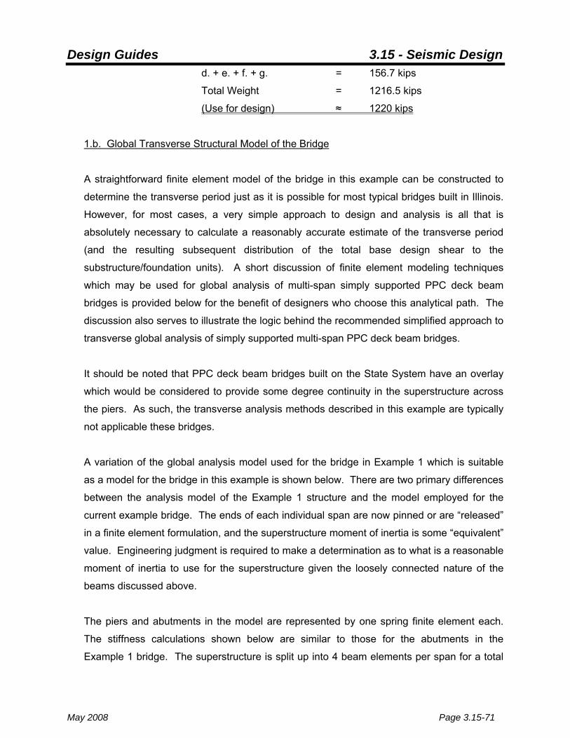
Design Guides 3.15 - Seismic Design
May 2008 Page 3.15-71
d. + e. + f. + g. = 156.7 kips
Total Weight = 1216.5 kips
(Use for design) ≈ 1220 kips
1.b. Global Transverse Structural Model of the Bridge
A straightforward finite element model of the bridge in this example can be constructed to
determine the transverse period just as it is possible for most typical bridges built in Illinois.
However, for most cases, a very simple approach to design and analysis is all that is
absolutely necessary to calculate a reasonably accurate estimate of the transverse period
(and the resulting subsequent distribution of the total base design shear to the
substructure/foundation units). A short discussion of finite element modeling techniques
which may be used for global analysis of multi-span simply supported PPC deck beam
bridges is provided below for the benefit of designers who choose this analytical path. The
discussion also serves to illustrate the logic behind the recommended simplified approach to
transverse global analysis of simply supported multi-span PPC deck beam bridges.
It should be noted that PPC deck beam bridges built on the State System have an overlay
which would be considered to provide some degree continuity in the superstructure across
the piers. As such, the transverse analysis methods described in this example are typically
not applicable these bridges.
A variation of the global analysis model used for the bridge in Example 1 which is suitable
as a model for the bridge in this example is shown below. There are two primary differences
between the analysis model of the Example 1 structure and the model employed for the
current example bridge. The ends of each individual span are now pinned or are “released”
in a finite element formulation, and the superstructure moment of inertia is some “equivalent”
value. Engineering judgment is required to make a determination as to what is a reasonable
moment of inertia to use for the superstructure given the loosely connected nature of the
beams discussed above.
The piers and abutments in the model are represented by one spring finite element each.
The stiffness calculations shown below are similar to those for the abutments in the
Example 1 bridge. The superstructure is split up into 4 beam elements per span for a total

Design Guides 3.15 - Seismic Design
Page 3.15-72 May 2008
of 12. A discussion on estimating the superstructure transverse moment of inertia (stiffness)
is also provided below.
kAbut kAbutkPier kPier
IEquivalent Transverse Superstructure
40 ft. = 480 in. 60 ft. = 720 in. 40 ft. = 480 in.
140 ft. = 1680 in.
kAbut kAbutkPier kPier
IEquivalent Transverse Superstructure
40 ft. = 480 in. 60 ft. = 720 in. 40 ft. = 480 in.
140 ft. = 1680 in.
1.c. Transverse Pier Stiffness
The stiffness calculation method for the pile bent pier is directly analogous to Example 1
Part 1.d. except that the height of each pile (column in and above soil) is from the depth-of-
fixity to the bottom of the pier cap. Note that the individual encasements of the piles are not
considered structural. The soil type is Class D.
Piles HP 12 x 53
Number of Piles 7
Weak Axis Pile Moment of Inertia Ip = 127 in.4
(Typical Orientation for Illinois)
Steel Modulus of Elasticity Es = 29000 ksi
Pile Depth-of-Fixity (Fixed-Fixed) 7.3 ft. = 87.6 in.
(from Geotechnical Analysis-
see also Appendix C)
Pile Height Ground to Cap Bottom 6.0 ft. = 72 in.
Total Pile (Column) Height 159.6 in.
Stiffness of Pier h
IE12 piles) .no(k 3
p
psPier
×××=

Design Guides 3.15 - Seismic Design
May 2008 Page 3.15-73
in.k
3Pier 1.766.159
1272900012 7k =×××
=
1.d. Transverse Abutment Stiffness
The stiffness calculation method for the abutment is identical to Example 1 Part 1.d. The
soil type is Class D.
Piles HP 10 x 42
Number of Piles 5
Weak Axis Pile Moment of Inertia Ip = 71.7 in.4
(Typical Orientation for Illinois)
Steel Modulus of Elasticity Es = 29000 ksi
Pile Depth-of-Fixity (Fixed-Fixed) 6.7 ft. = 80.4 in.
(from Geotechnical Analysis-
see also Appendix C)
Stiffness of Abutment h
IE12 piles) .no(k 3
p
psAbut
×××=
in.k
3Abut 0.2404.80
7.712900012 5k =×××
=
1.e. Transverse Superstructure Stiffness
The beams should only be considered as contributing to the transverse moment of inertia of
superstructure. However, the beams are only loosely tied together with several rods which
are not post tensioned. A “fully effective” transverse moment of inertia for the superstructure
can be calculated as given below.
Area of 1 Beam 702 in.2
Moment of Inertia of Deck ( ) 47222
n
1i
2iBeam
.in 105.41442962482702
(in.) centroid from distance d beams, of .no n ,dA
×=×+×+×=
==∑=
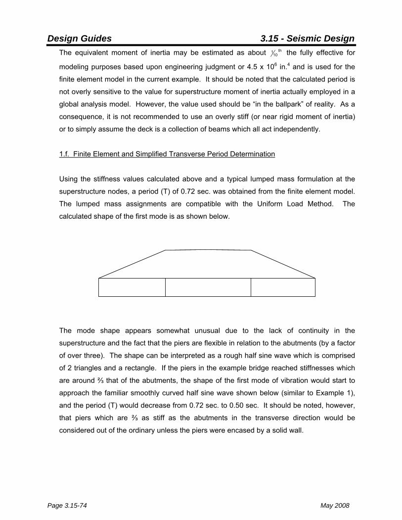
Design Guides 3.15 - Seismic Design
Page 3.15-74 May 2008
The equivalent moment of inertia may be estimated as about th10
1 the fully effective for
modeling purposes based upon engineering judgment or 4.5 x 106 in.4 and is used for the
finite element model in the current example. It should be noted that the calculated period is
not overly sensitive to the value for superstructure moment of inertia actually employed in a
global analysis model. However, the value used should be “in the ballpark” of reality. As a
consequence, it is not recommended to use an overly stiff (or near rigid moment of inertia)
or to simply assume the deck is a collection of beams which all act independently.
1.f. Finite Element and Simplified Transverse Period Determination
Using the stiffness values calculated above and a typical lumped mass formulation at the
superstructure nodes, a period (T) of 0.72 sec. was obtained from the finite element model.
The lumped mass assignments are compatible with the Uniform Load Method. The
calculated shape of the first mode is as shown below.
The mode shape appears somewhat unusual due to the lack of continuity in the
superstructure and the fact that the piers are flexible in relation to the abutments (by a factor
of over three). The shape can be interpreted as a rough half sine wave which is comprised
of 2 triangles and a rectangle. If the piers in the example bridge reached stiffnesses which
are around ⅔ that of the abutments, the shape of the first mode of vibration would start to
approach the familiar smoothly curved half sine wave shown below (similar to Example 1),
and the period (T) would decrease from 0.72 sec. to 0.50 sec. It should be noted, however,
that piers which are ⅔ as stiff as the abutments in the transverse direction would be
considered out of the ordinary unless the piers were encased by a solid wall.
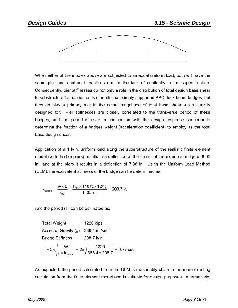
Design Guides 3.15 - Seismic Design
May 2008 Page 3.15-75
When either of the models above are subjected to an equal uniform load, both will have the
same pier and abutment reactions due to the lack of continuity in the superstructure.
Consequently, pier stiffnesses do not play a role in the distribution of total design base shear
to substructure/foundation units of multi-span simply supported PPC deck beam bridges, but
they do play a primary role in the actual magnitude of total base shear a structure is
designed for. Pier stiffnesses are closely correlated to the transverse period of these
bridges, and the period is used in conjunction with the design response spectrum to
determine the fraction of a bridges weight (acceleration coefficient) to employ as the total
base design shear.
Application of a 1 k/in. uniform load along the superstructure of the realistic finite element
model (with flexible piers) results in a deflection at the center of the example bridge of 8.05
in., and at the piers it results in a deflection of 7.88 in. Using the Uniform Load Method
(ULM), the equivalent stiffness of the bridge can be determined as,
in.kft.
in..in
k
MaxBridge 208.7
in. 05.812 ft. 1401Lwk =
××=
δ×
=
And the period (T) can be estimated as,
Total Weight 1220 kips
Accel. of Gravity (g) 386.4 in./sec.2
Bridge Stiffness 208.7 k/in.
sec. 77.07.2084.386
12202kgW2T
Bridge
=×
π=×
π=
As expected, the period calculated from the ULM is reasonably close to the more exacting
calculation from the finite element model and is suitable for design purposes. Alternatively,

Design Guides 3.15 - Seismic Design
Page 3.15-76 May 2008
the transverse period can also be calculated (estimated) using the Uniform Load Method
assuming that the maximum deflection occurs at the piers as follows.
in.kft.
in..in
k
PierBridge 213.2
in. 88.712 ft. 1401Lwk =
××=
δ×
= (Eq. 1)
sec. 76.02.2134.386
12202kgW2T
Bridge
=×
π=×
π= (Eq. 2)
This alternative method also produces a reasonably accurate period which is suitable for
design. Since the reactions for multi-span simply supported PPC deck beam bridges can be
calculated according to the tributary span lengths framing into substructure/foundation units,
the pier deflections for a 1 k/in. uniform load applied to the bridge can be calculated as
follows.
Pier Reactions ( )( )( ) kips 600112ft. 60ft. 40RR .ink
.ft.in
21
21
2P1P =×+×== (Eq. 3)
Pier Deflections in. 88.71.76kips 600
.ink2P1P ==δ=δ (Eq. 4)
As can be seen from the above derivation, sophisticated analytical techniques such as finite
element modeling are not necessary to determine the period for most bridges which are in
the same class as the bridge in the current example. A summary of the steps required to
determine the period for most multi-span simply supported PPC deck beam bridges,
typically up to 5 spans, is given below (simplified method) along with some discussion on
their potential limitations.
1. Determine the transverse stiffnesses for each pier according to 1.c.
2. Determine the transverse stiffnesses for each abutment according to 1.d.
3. Compare the relative differences between the stiffnesses of the abutments and the
piers. The abutments should be around two to three times stiffer than the piers at a
minimum, but this is not absolutely required.
Design Guides 3.15 - Seismic Design
May 2008 Page 3.15-77
4. Compare the relative differences between the stiffnesses of the piers. If there are
significant differences in stiffness from pier to pier, the period calculated from this
method may be overly conservative, but it is still suitable for design purposes.
5. Using the stiffest pier, calculate the reaction according the tributary span length
method described by Eq. 3 with a uniform load of 1 k/in.
6. Using the reaction calculated in Step 5, determine the deflection of the pier according
the method described by Eq. 4.
7. Using the method described by Eq. 1, calculate the equivalent stiffness of the bridge.
8. Using the method describe by Eq. 2, calculate the period (T) of the bridge.
2. Determination of Bridge Period – Longitudinal Direction
2.a. Weight and Global Longitudinal Structural Model of the Bridge The methods required to determine the longitudinal period of multi-span simply supported
PPC deck beam bridges are similar to those described in Example 1. The mass of the
bridge used for calculation of the longitudinal period is the same as that used for the
transverse direction. For bridges in the class of the current example structure, it is
recommended that the longitudinal stiffnesses of all piers and abutments be used in the
structural modeling and calculation of the period. Even though each span in the
superstructure is simply supported; the ends of the spans are in close proximity, and seismic
loads will be transmitted through the superstructure before the “fixed” dowel bars fuse and
afterward through friction due to adequate seat widths. As such, the superstructure across
the entire length of the bridge will essentially behave as one rigid body which transfers
seismic loads to the substructures/foundations in a similar manner to bridges which have
continuous superstructures. In addition, due to the nature of the configuration of bridges in
this class (i.e. typically flexible piers), it is beneficial (and required in some cases) to rely
upon the structural resistance of the abutments to absorb seismic loads in order to produce
designs that are feasible.

Design Guides 3.15 - Seismic Design
Page 3.15-78 May 2008
2.b. Longitudinal Pier Stiffness
The piles (columns) for individually encased pile bent piers should be assumed to deflect as
cantilevers which deform from “fixed ends” (at the depth-of-fixity in soil) to the bottom of the
cap beam. The rigid body rotation of the cap should also be included in the stiffness
determination. The equations and derivation below determine the stiffness, and the figure
provides an illustration for guidance for one pile in a bent.
Pile Stiffness w/o Cap cap of bottom tofixity -of
-depth as taken height h where; h
IE3k p3
p
psp =
××=
kp = 3 x Es x Ip / hp3
hp
hCapCap Beamk = ∞
Pile Stiffness
Cap Beamk =
Seismic Load
kp = 3 x Es x Ip / hp3
hp
hCapCap Beamk = ∞
Pile Stiffness
Cap Beamk =
Seismic Load
Pile Stiffness w/ Cap
TDPile per Pier Long
ATpTD
TpCapA
A
ps
2p
Tp
Tp
ps
3p
pTpTpp
Tp
Pk
:is then stiffness long. pile pierfinal the and is , ,deflection total The
h:is , beam, cap
the of top the at pier the of deflection added The
IE2hP
:is , pile, a of top the at rotation the P, load a For
IE3hP
kP Pk
:is , pile, a of top the at deflection the P, load a For
δ=
δ+δδ
θ×=δ
δ
××
×=θ
θ
××
×==δ⇒=δ×
δ

Design Guides 3.15 - Seismic Design
May 2008 Page 3.15-79
For a simple global stiffness analysis, the depth-of-fixity based upon deflection and not
moment should be used for the fixed-pinned case. Appendix C provides depths-of-fixity in
terms of moment. For the fixed-pinned case, the depths-of-fixity based upon deflection are
about twice that for moment as discussed in Appendix C. The stiffness of the piers for the
current example is given below.
Piles HP 12 x 53
Number of Piles 7
Stong Axis Pile Moment of Inertia Ip = 393 in.4
(Typical Orientation for Illinois)
Steel Modulus of Elasticity Es = 29000 ksi
Pile Depth-of-Fixity (Fixed-Pinned) 2 x 4.9 ft. = 9.8 ft. = 117.6 in.
(from Geotechnical Analysis-
see also Appendix C)
Pile Height Ground to Cap Bottom 6.0 ft. = 72 in.
Total Pile (Column) Height 189.6 in.
Stiffness of Piles w/o Cap h
IE3 piles) .no(k 3
p
psP
×××=
in.k
3P 1.356.189
393290003 7k =×××
=
Stiffness of Pier
w/ Cap
in.k
TD Pier Long
ATPTD
TD
TPCapA
A
2
TP
TP
TPTPP
TP
4.28Pk
:is cap withstiffness column The
0.035249P0.0067590P0.028490P :deflection total the ,
P0067590.0P00022530.0in. 30h:cap of top the at deflection added the ,
P00022530.03932900027
6.189P:P load a for piles of top at rotation ,
P028490.01.35P Pk
:P load a for piles of top at deflection
=δ=
=+=δ+δ=δ
δ
=×=θ×=δ
δ
=×××
×=θ
θ
==δ⇒=δ×
δ
Design Guides 3.15 - Seismic Design
Page 3.15-80 May 2008
2.c. Longitudinal Abutment Stiffness
The stiffness of the abutments is calculated in the same way as the piers with the exception
that the piles are not exposed to air. As such, the abutments have shorter effective heights
and are stiffer than the piers.
Piles HP 10 x 42
Number of Piles 5
Stong Axis Pile Moment of Inertia Ip = 210 in.4
(Typical Orientation for Illinois)
Steel Modulus of Elasticity Es = 29000 ksi
Pile Depth-of-Fixity (Fixed-Pinned) 2 x 4.4 ft. = 8.8 ft. = 105.6 in.
(from Geotechnical Analysis-
see also Appendix C)
Stiffness of Piles w/o Cap h
IE3 piles) .no(k 3
p
psA
×××=
in.k
3A 6.776.105
210290003 5k =×××
=
Stiffness of Abutment
w/ Cap
in.k
TD AbutLong
ATATD
TD
TACapA
A
2
TA
TA
TATAA
TA
4.54Pk
:is cap withstiffness column The
0.018380P0.0054933P0.012887P :deflection total the ,
P0054933.0P00018311.0in. 30h:cap of top the at deflection added the ,
P00018311.02102900025
6.105P:P load a for piles of top at rotation ,
P012887.06.77P Pk
:P load a for piles of top at deflection
=δ=
=+=δ+δ=δ
δ
=×=θ×=δ
δ
=×××
×=θ
θ
==δ⇒=δ×
δ
Design Guides 3.15 - Seismic Design
May 2008 Page 3.15-81
2.d. Uniform Load Method Longitudinal Period Determination
The Uniform Load Method is used in the current example to straightforwardly calculate the
longitudinal bridge period with the equation given below.
bridge of massM where;k2k2
M2TAbut LongPier Long
=×+×
π=
Mass of Bridge .in.seck 21573.3
4.3861220
gBridge of WeightM −===
Period sec. 87.04.5424.282
1573.32T =×+×
π=
3. Determination of Base Shears – 1000 Year Design Earthquake Return Period
3.a. Design Response Spectrum (LRFD)
Reference Appendix 3.15.A of the Bridge Manual and Section 3 of the LRFD Code for more
information on the formulation of the 1000 yr. Design Response Spectrum.
The bridge in this example is geographically located at the upper acceleration boundary of
Zone 2 with Class D Soil (which is common in Southern Illinois). The map shown below is
repeated from the Bridge Manual. It illustrates (approximately) the seismicity of Illinois for
Class D soil. An examination of the map reveals that the bridge in the current example is
being designed for moderate to high seismicity. This is also an area of the State for which
PPC deck beam bridges are commonly constructed on the Local System.

Design Guides 3.15 - Seismic Design
Page 3.15-82 May 2008

Design Guides 3.15 - Seismic Design
May 2008 Page 3.15-83
The following are the seismic design data for the current example bridge.
Ss (Short Period Acceleration) 0.50g (See LRFD Code Maps Article 3.10.2.1)
S1 (1-Sec. Period Acceleration) 0.13g (See LRFD Code Maps Article 3.10.2.1)
Soil Type Class D (In Upper 100 ft. of Soil Profile)
Fa (Short Period Soil Coef.) 1.40 (BM Table 3.15.A.2.3-1)
Fv (1-sec. Period Soil Coef.) 2.28 (BM Table 3.15.A.2.3-2)
SDS g70.05.04.1SF sa =×=
SD1 g30.013.028.2SF 1v =×=
Seismic Performance Zone 2 ( )1-3.15.2 Table BM 30.0SF15.0 1v ≤<
Importance Category Other (Flexible Option according to BM Section
3.15.8)
Definitions and a graphical representation of the design response spectrum (with
approximate acceleration at zero sec. period) are given below.
0
1.6
0 1 2
SDS = FaSs
SD1 = FvS1
TSS 1D
a =
0.4SDS
Period, T (sec.)
Res
pons
e Sp
ectr
al A
ccel
erat
ion,
Sa
1.00.2
DS
1Ds S
ST =
s0 T2.0T =
0
1.6
0 1 2
SDS = FaSs
SD1 = FvS1
TSS 1D
a =
0.4SDS
Period, T (sec.)
Res
pons
e Sp
ectr
al A
ccel
erat
ion,
Sa
1.00.2
DS
1Ds S
ST =
s0 T2.0T =
Ts = 429.07.03.0 = sec.
T0 = 086.0429.02.0 =× sec.
Less than T0, Sa = 28.0T88.4S4.0TT
S6.0 DS
0
DS +=+

Design Guides 3.15 - Seismic Design
Page 3.15-84 May 2008
Greater than Ts, Sa = T30.0
(Where T = Tm, and Sa = Csm in the LRFD Code)
Transverse Direction:
Sa (Csm in the LRFD Code) = 76.030.0 = 0.39 (T = 0.76 > Ts = 0.429 sec.)
Longitudinal Direction:
Sa (Csm in the LRFD Code) = 87.030.0 = 0.34 (T = 0.87 > Ts = 0.429 sec.)
Values beyond the “plateau” (analogous to 2.5A in the LFD Code) are not unexpected in the
transverse and longitudinal directions for many typical multi-span simply supported PPC
deck beam bridges.
3.b. Transverse Base Shear
Total Base Shear = kips 8.47512200.39 Bridge of .WtSa =×=×
Or in.k 283.0in.1680
kips 475.8 =
As discussed above, the transverse seismic base shear is distributed to the piers and
abutments according to the simple tributary span lengths which frame into these
substructure/foundation units.
VBase Shear P (T) = ( ) kips 8.169in 720 in. 480283.0 21
21
.ink =×+×
VBase Shear A (T) = ( ) kips 9.67in. 480283.0 21
.ink =×
3.c. Longitudinal Base Shear
Total Base Shear = kips 8.41412200.34 Bridge of .WtSa =×=×

Design Guides 3.15 - Seismic Design
May 2008 Page 3.15-85
For this example, the longitudinal seismic base shear is distributed to the piers and
abutments according to the relative stiffnesses of these units.
VBase Shear P (L) = ( ) kips 8.4144.5424.282
4.28.in
k
.ink
××+×
= 71.1 kips
VBase Shear A (L) = ( ) kips 8.4144.5424.282
4.54.in
k
.ink
××+×
= 136.3 kips
4. Frame Analysis and Pile (Columnar) Seismic Forces for Pile Bents
4.a. Pier Forces – Dead Load
Dead Load of Superstructure
(Use Wt. from Previous Calculations) = 1220 kips
Bridge Length = 140 ft.
Dead Load Per ft. of Bridge = .ftk714.8140
1220 =
Dead Load Per Pier (Use Statics) = ⎟⎠⎞
⎜⎝⎛ +× CenterSpanOuterSpan L
21L
21714.8
= kips 7.435602140
21714.8 =⎟
⎠⎞
⎜⎝⎛ ×+××
No. of Piles (Columns) Per Pier = 7
Dead Load Per Pile = kips 2.6277.435 =
Added Dead Load for Bot. Half of 1 Col.
Not Considered in Pt. 1.a. Sub-Pt. e. = Neglect as not significant
4.b. Pier Forces – Transverse Overturning
The seismic base shear at each pier theoretically acts through the centroid of the
superstructure. It is acceptable to assume/approximate that the centroid acts at the top of
the beams. From statics, shown below, an “overturning moment” produces axial

Design Guides 3.15 - Seismic Design
Page 3.15-86 May 2008
compression and tension across the bent assuming a connection which resists uplift
between the superstructure and the substructures. The seismic base shear also produces
“frame action” forces in the piles (columns) of the bent and acts at the bottom of the cap (the
“eccentricity” or “arm” of the base shear is taken into account through consideration of the
overturning moment) Frame action force analysis is given in the following section.
Appendix A contains overturning moment solutions for bents with 2 to 13 columns. In
reality, for multi-span simply supported PPC deck beam structures, the axial compressive
forces predicted from the simple overturning moment solutions are probably more accurate
than the predicted tensile forces due to the nature of the connection between the
superstructures and substructures for this class of bridges. However, the solutions give
results which are suitable for design purposes.
Sp
d
PSTarm
0.67PST
PST
0.67PST
( )( )( )
dM107.0P
dP33.02 d2P67.02
d3P2MarmSM
ST
ST
ST
ST
p
=∴
×
+×
+×=
×=0.33PST0.33PST
0
d d d d d
Sp
d
PSTarm
0.67PST
PST
0.67PST
( )( )( )
dM107.0P
dP33.02 d2P67.02
d3P2MarmSM
ST
ST
ST
ST
p
=∴
×
+×
+×=
×=0.33PST0.33PST
0
d d d d d
Sp (Base Shear at Pier) = 169.8 kips
arm (Base Shear Eccentricity)
Cap Height + Beam Height = ft. 75.412/275.2 =+
d (Center-to-Center Pile Distance) = 4 ft. – 2 in. = 4.17 ft.
M (Overturning Moment) = ft.-k 6.80675.48.169 =×
PST (Maximum Axial Columnar Force) = kips 7.2017.46.806107.0 =×

Design Guides 3.15 - Seismic Design
May 2008 Page 3.15-87
4.c. Pier Forces – Transverse Frame Action
Taking account of the overturning moment “transfers” the seismic base shear at the pier to
the tops of the piles (columns). This shear produces moments, shears and axial forces in
each pile of the bent through “frame action.” Free body diagram solutions for these seismic
forces are shown below. The determination of moment and shear in each column is more
straightforward than for axial force. The simple solutions for moment in the piles are very
accurate while conservative solutions for axial force due frame action are emphasized for
the critical outside piles. Appendix B contains frame action columnar axial force solutions
for bents with 2 to 6 or more columns.
2hVM ST
ST×=
VST
VST
MST
MST
d
VST VST VST
h
7SV P
ST =
VSTVST VSTVST VST
2hVM ST
ST×=
VST
VST
MST
MST
d
VST VST VST
h
7SV P
ST =
VSTVST VSTVST VST
Sp (Base Shear at Pier) = 169.8 kips
Column Height (Fixity to Cap Bot.) = 13.3 ft.
VST (Shear Per Pile) = kips 3.2478.169 =
MST (Moment Per Pile) = ft.-k 6.16123.133.24 =×
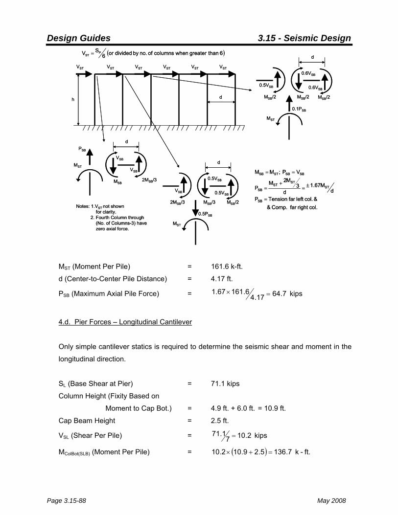
Design Guides 3.15 - Seismic Design
Page 3.15-88 May 2008
d
col. right far Comp. & & col. left far Tension P
dM67.1
d3
M2MP
VP ;MM
SB
STST
STSB
SBSBSTSB
=
±=+
=
==
VST VST VST
MST
h
MSB2MSB/3
VSB
VSB
PSB
d
Notes: 1.VST not shownfor clarity.
2. Fourth Column through (No. of Columns-3) have zero axial force.
( )6 than greater whencolumns of no.by divided or 6SV P
ST =
VST
2MSB/3 MSB/3
0.5VSB
VSB
d
MST
0.5PSB
MSB/2
0.5VSB
MSB/2 MSB/2
0.6VSB
0.5VSB
d
MST
0.6VSB
VST
MSB/2
VST
0.1PSB
d
col. right far Comp. & & col. left far Tension P
dM67.1
d3
M2MP
VP ;MM
SB
STST
STSB
SBSBSTSB
=
±=+
=
==
VST VST VST
MST
h
MSB2MSB/3
VSB
VSB
PSB
d
Notes: 1.VST not shownfor clarity.
2. Fourth Column through (No. of Columns-3) have zero axial force.
( )6 than greater whencolumns of no.by divided or 6SV P
ST =
VST
2MSB/3 MSB/3
0.5VSB
VSB
d
MST
0.5PSB
MSB/2
0.5VSB
MSB/2 MSB/2
0.6VSB
0.5VSB
d
MST
0.6VSB
VST
MSB/2
VST
0.1PSB
MST (Moment Per Pile) = 161.6 k-ft.
d (Center-to-Center Pile Distance) = 4.17 ft.
PSB (Maximum Axial Pile Force) = kips 7.6417.46.16167.1 =×
4.d. Pier Forces – Longitudinal Cantilever
Only simple cantilever statics is required to determine the seismic shear and moment in the
longitudinal direction.
SL (Base Shear at Pier) = 71.1 kips
Column Height (Fixity Based on
Moment to Cap Bot.) = 4.9 ft. + 6.0 ft. = 10.9 ft.
Cap Beam Height = 2.5 ft.
VSL (Shear Per Pile) = kips 2.1071.71 =
MColBot(SLB) (Moment Per Pile) = ( ) ft.-k 7.1365.29.102.10 =+×

Design Guides 3.15 - Seismic Design
May 2008 Page 3.15-89
5. Frame Analysis and Pile (Columnar) Seismic Forces for Abutments
The analysis of the abutments for seismic forces is directly analogous to that of the piers.
5.a. Abutment Forces – Dead Load
Dead Load of Superstructure
(Use Wt. from Previous Calculations) = 1220 kips
Bridge Length = 140 ft.
Dead Load Per ft. of Bridge = .ftk714.8140
1220 =
Dead Load Per Abut. (Use Statics) = ⎟⎠⎞
⎜⎝⎛× OuterSpanL
21714.8
= kips 3.1744021714.8 =⎟
⎠⎞
⎜⎝⎛ ××
No. of Piles (Columns) Per Abut. = 5
Dead Load Per Pile = kips 9.3453.174 =
5.b. Abutment Forces – Transverse Overturning
Sp
d
PSTarm0.5PST
PST
0.5PST
( )( )
dM
51P
dP2 d2P2M
armSM
ST
ST21ST
p
=∴
×
+×=
×=
d d d
0
Sp
d
PSTarm0.5PST
PST
0.5PST
( )( )
dM
51P
dP2 d2P2M
armSM
ST
ST21ST
p
=∴
×
+×=
×=
d d d
0

Design Guides 3.15 - Seismic Design
Page 3.15-90 May 2008
Sp (Base Shear at Abutment) = 67.9 kips
arm (Base Shear Eccentricity)
Cap Height + Beam Height = ft. 75.412/275.2 =+
d (Center-to-Center Pile Distance) = 6 ft. – 3 in. = 6.25 ft.
M (Overturning Moment) = ft.-k 5.32275.49.67 =×
PST (Maximum Axial Columnar Force) = kips 10.3 25.65.322
51
=×
5.c. Abutment Forces – Transverse Frame Action
d d 2hVM ST
ST×=
VST VST VST
VST
VST
MST
MST
h
5SV P
ST =
d
VST
d
VST
d
VST
d d 2hVM ST
ST×=
VST VST VST
VST
VST
MST
MST
h
5SV P
ST =
d
VST
d
VST
d
VST
Sp (Base Shear at Abutment) = 67.9 kips
Column Height (Fixity to Cap Bot.) = 6.7 ft.
VST (Shear Per Pile) = kips 6.1359.67 =
MST (Moment Per Pile) = ft.-k 6.4527.66.13 =×

Design Guides 3.15 - Seismic Design
May 2008 Page 3.15-91
d
col. right far Comp. & & col. left far Tension P
dM67.1
d3
M2MP
VP ;MM
SB
STST
STSB
SBSBSTSB
=
±=+
=
==
VST VST VST
MST
h
MSB2MSB/3
VSB
VSB
PSB
d
Note: VST not shown for clarity
5SV P
ST =
VST
2MSB/3 MSB/3
0.5VSB
VSB
d
MST
0.5PSB
MSB/2
0.5VSB
MSB/2 MSB/2
0.5VSB
0.5VSB
d
MST
0.0
0.5VSB
VST
MSB/3d
col. right far Comp. & & col. left far Tension P
dM67.1
d3
M2MP
VP ;MM
SB
STST
STSB
SBSBSTSB
=
±=+
=
==
VST VST VST
MST
h
MSB2MSB/3
VSB
VSB
PSB
d
Note: VST not shown for clarity
5SV P
ST =
VST
2MSB/3 MSB/3
0.5VSB
VSB
d
MST
0.5PSB
MSB/2
0.5VSB
MSB/2 MSB/2
0.5VSB
0.5VSB
d
MST
0.0
0.5VSB
VST
MSB/3
MST (Moment Per Pile) = 45.6 k-ft.
d (Center-to-Center Pile Distance) = 6.25 ft.
PSB (Maximum Axial Pile Force) = kips 2.1225.66.4567.1 =×
5.d. Abutment Forces – Longitudinal Cantilever
SL (Base Shear at Abutment) = 136.3 kips
Column Height (Fixity Based on
Moment to Cap Bot.) = 4.4 ft.
Cap Beam Height = 2.5 ft.
VSL (Shear Per Pile) = kips 3.2753.136 =
MColBot(SLB) (Moment Per Pile) = ( ) ft.-k 4.1885.24.43.27 =+×
Design Guides 3.15 - Seismic Design
Page 3.15-92 May 2008
6. Seismic Design Forces for Pile Bent Including R-Factor, P-Δ, and Combination of
Orthogonal Forces
6.a. R-Factor
R-Factors should only be used to reduce the moments calculated from the base shears of
an “elastic” analysis as was conducted above. As recommended in the Bridge Manual
(Section 3.15.8) an R-Factor of 3.5 will be used for the pile bents in this example. This
coincides with classifying the bridge as “Other” according to the LRFD Code.
6.b. P-Δ
See Example 1 Part 6.b. for discussion on this topic. For the current example bridge, a 5%
amplification of bending moments will be used to account for P-Δ effects.
6.c. Summary and Combination of Orthogonal Column Forces Used for Design
The forces on the two exterior piles (columns) in the example bridge are focused on for
design because they experience the most extreme earthquake forces. The pier piles should
be designed for the possibility of earthquake accelerations which can be in opposite
transverse directions and opposite longitudinal directions. They are also required to be
designed for the cases “mostly longitudinal and some transverse accelerations”
(Longitudinal Dominant – Load Case 1) and “some longitudinal and mostly transverse
accelerations” (Transverse Dominant – Load Case 2).
Since the bridge in this example is not skewed, the combination of orthogonal forces used
for design is straightforward. More complex cases with skew and non-round columns are
considered in Examples 2 and 3 of this design guide. The equations below present the
basic method for combination of orthogonal forces.
Load Case 1 (Longitudinal Dominant) Load Case 2 (Transverse Dominant)
Tz
Lz
Dz V3.0V0.1V += T
zLz
Dz V0.1V3.0V +=

Design Guides 3.15 - Seismic Design
May 2008 Page 3.15-93
Ty
Ly
Dy V3.0V0.1V += T
yLy
Dy V0.1V3.0V +=
Tz
Lz
Dz M3.0M0.1M += T
zLz
Dz M0.1M3.0M +=
Ty
Ly
Dy M3.0M0.1M += T
yLy
Dy M0.1M3.0M +=
TLD P3.0P0.1P += TLD P0.1P3.0P +=
For the bridge in this example the Longitudinal- and z-axes, and Transverse- and y-axes
coincide as shown below.
40 ft. 60 ft. 40 ft.
L, z
T, y
L, z
T, y
40 ft. 60 ft. 40 ft.
L, z
T, y
L, z
T, y
Shown below are the Load Case 1 and Load Case 2 forces used for seismic design with R-
Factor (3.5), P-Δ amplification (1.05), and axial dead load (62.2 kips) effects all considered.
Load Case 1 – Longitudinal Dominant (per pile):
kips 2.102.100.103.0V0.1V3.0V0.1V SLTz
Lz
Dz ==+=+=
kips 3.73.243.0V3.000.1V3.0V0.1V STTy
Ly
Dy ==+=+=
ft.-k 5.145.36.16105.13.05.3
M05.13.000.1M3.0M0.1M STTz
Lz
Dz =×=×+=+=
ft.-k 0.415.37.13605.10.103.05.3
M05.10.1M3.0M0.1M SLBTy
Ly
Dy =×=+×=+=

Design Guides 3.15 - Seismic Design
Page 3.15-94 May 2008
kips 8.87 and 6.36
7.647.203.02.62PP3.000.1PPP3.0P0.1P SBSTDeadDTLD
=
=+±=+±+=→+=
Note that the Department recommends a load factor of 1.0 be used for dead loads for
LRFD.
Load Case 2 – Transverse Dominant (per pile):
kips 1.32.103.000.1V3.0V0.1V3.0V SLTz
Lz
Dz ==+=+=
kips 24.33.240.1V0.103.0V0.1V3.0V STTy
Ly
Dy ==+=+=
ft.-k 5.485.36.16105.10.15.3
M05.10.103.0M0.1M3.0M STTz
Lz
Dz =×=×+=+=
ft.-k 3.125.37.13605.13.000.15.3
M05.13.0M0.1M3.0M SLBTy
Ly
Dy =×=+×=+=
kips 147.6 and (Ten.) 2.23
7.647.200.12.62PP0.103.0PPP0.1P3.0P SBSTDeadDTLD
−=
=+±=+±+=→+=
7. Seismic Design Forces for Abutment Including R-Factor, P-Δ, and Combination of
Orthogonal Forces
7.a. R-Factor
As recommended in the Bridge Manual (Section 3.15.8) an R-Factor of 1.5 will be used for
the piles supporting the stub abutments in this example. This coincides with classifying the
bridge as “Other” according to the LRFD Code.
7.b. P-Δ
P-Δ effects should be ignored for piles at abutments.
7.c. Summary and Combination of Orthogonal Column Forces Used for Design
The method for combining of orthogonal forces for the abutments is similar to that for the
piers. Shown below are the Load Case 1 and Load Case 2 forces used for seismic design

Design Guides 3.15 - Seismic Design
May 2008 Page 3.15-95
with R-Factor (1.5), P-Δ amplification (1.00), and axial dead load (34.9 kips) effects all
considered.
Load Case 1 – Longitudinal Dominant (per pile):
kips 3.273.270.103.0V0.1V3.0V0.1V SLTz
Lz
Dz ==+=+=
kips 1.46.133.0V3.000.1V3.0V0.1V STTy
Ly
Dy ==+=+=
ft.-k 1.95.16.4500.13.00.2
M00.13.000.1M3.0M0.1M STTz
Lz
Dz =×=×+=+=
ft.-k 6.1255.14.18800.10.103.00.2
M00.10.1M3.0M0.1M SLBTy
Ly
Dy =×=+×=+=
kips 7.41 and 2.28
2.123.103.09.34PP3.000.1PPP3.0P0.1P SBSTDeadDTLD
=
=+±=+±+=→+=
Note that the Department recommends a load factor of 1.0 be used for dead loads for
LRFD.
Load Case 2 – Transverse Dominant (per pile):
kips 2.83.273.000.1V3.0V0.1V3.0V SLTz
Lz
Dz ==+=+=
kips 13.66.130.1V0.103.0V0.1V3.0V STTy
Ly
Dy ==+=+=
ft.-k 4.305.16.4500.10.10.2
M00.10.103.0M0.1M3.0M STTz
Lz
Dz =×=×+=+=
ft.-k 7.375.14.18800.13.000.10.2
M00.13.0M0.1M3.0M SLBTy
Ly
Dy =×=+×=+=
kips 57.4 and 4.12
2.123.100.19.34PP0.103.0PPP0.1P3.0P SBSTDeadDTLD
=
=+±=+±+=→+=
8. Combined Axial Force and Bi-Axial Bending Structural Capacity Check for Piles in
Bents
The piles should be checked for structural capacity using Articles 6.8 (Tension Members) or
Article 6.9 (Compression Members) of the LRFD Code for combined axial force and bi-axial

Design Guides 3.15 - Seismic Design
Page 3.15-96 May 2008
bending. Note that all φ factors according to LRFD Article 6.5.5 shall be taken as 1.0 for
extreme events.
Geotechnical considerations for the design of piles to resist seismic loadings are provided in
Sections 3.10 and 3.15 of the Bridge Manual as well as Design Guide 3.10.1. Guidance on
liquefaction, lateral pile resistance in soil, pullout from the soil, etc. are among the
considerations addressed.
8.a. Load Case 1 – Longitudinal Dominant
Both axial forces for Load Case 1 are compressive. LRFD Article 6.9.2.2 contains the
provisions for checking axial compression in combination with bi-axial bending and shall
satisfy,
For 2.0PP
r
u < ,
0.1MM
MM
P0.2P
ry
uy
rx
ux
r
u ≤⎟⎟⎠
⎞⎜⎜⎝
⎛++ (Eq. 6.9.2.2-1)
Otherwise,
0.1MM
MM
98
PP
ry
uy
rx
ux
r
u ≤⎟⎟⎠
⎞⎜⎜⎝
⎛++ (Eq. 6.9.2.2-2)
Where:
Mux = design seismic moment about y-axis of bent (k-ft. or k-in.)
Muy = design seismic moment about z-axis of bent (k-ft. or k-in.)
Mrx = FySx, yield strength times section modulus about strong axis of
pile (k-ft. or k-in.)
Mry = FySy, yield strength times section modulus about weak axis of
pile (k-ft. or k-in.)
Pu = design seismic compressive force (kips)
Pr = allowable compressive resistance according to LRFD Article
6.9.2.1 (kips)

Design Guides 3.15 - Seismic Design
May 2008 Page 3.15-97
Pr = φPn (Eq. 6.9.2.1-1)
Where:
For λ ≤ 2.25,
Pn = 0.66λFyAs (Eq. 6.9.4.1-1)
Otherwise,
Pn = λ
sy AF88.0 (Eq. 6.9.4.1-2)
In which:
λ = EF
rK y
2
s⎟⎟⎠
⎞⎜⎜⎝
⎛πl (Eq. 6.9.4.1-3)
Where:
φ = 1.0
As = gross area of section (in.2)
Fy = yield strength of steel (ksi)
E = modulus of elasticity of steel (ksi)
K = effective length factor
l = unbraced length (in.)
rs = radius of gyration about plane of buckling (in.)
For Load Case 1 (HP 12 x 53),
Mux = DyM = 41.0 k-ft.
Muy = DzM = 14.5 k-ft.
Mrx = FySx = in. 12ft. 13in. 8.66ksi 50 ×× = 278.3 k-ft.
Mry = FySy = in. 12ft. 13in. 1.21ksi 50 ×× = 87.9 k-ft.
Pu = PD (max.) = 87.8 kips
Pr = φPn = 1.0Pn

Design Guides 3.15 - Seismic Design
Page 3.15-98 May 2008
λ = EF
rK y
2
s⎟⎟⎠
⎞⎜⎜⎝
⎛πl
K = 1.5 (≈ avg. about weak and strong axis pile)
l = 159.6 in. (about weak axis, would be 130.8 in. about strong axis taking
depth-of-fixity based upon moment)
Fy = 50 ksi
E = 29000 ksi
rs = 2.86 in. (about weak axis)
As = 15.5 in.2
λ = 29000
5086.2
6.1595.1 2
⎟⎠⎞
⎜⎝⎛
π×× = 1.22
λ ≤ 2.25,
∴Pr = (1.0)0.66λFyAs = (1.0) 5.155066.0 22.1 ×× = 466.8 kips
And,
2.019.08.466
8.87PP
r
u <== ,
OK 0.141.09.875.14
3.2780.41
8.4660.28.87
MM
MM
P0.2P
ry
uy
rx
ux
r
u ≤=⎟⎠⎞
⎜⎝⎛ ++
×=⎟
⎟⎠
⎞⎜⎜⎝
⎛++∴
8.b. Load Case 2 – Transverse Dominant
One design axial force for Load Case 2 is compressive and one is tensile. However, the
tensile load is much smaller that the compressive force in absolute magnitude, and the
allowable tensile force in pure tension is generally greater than for compression. The
provisions for axial tension combined with bi-axial bending are similar to those for axial
compression. Therefore, only LRFD Article 6.9.2.2 need be checked for Load Case 2.
For Load Case 2 (HP 12 x 53),
Mux = DyM = 12.3 k-ft.
Muy = DzM = 48.5 k-ft.
Mrx = FySx = in. 12ft. 13in. 8.66ksi 50 ×× = 278.3 k-ft.
Design Guides 3.15 - Seismic Design
May 2008 Page 3.15-99
Mry = FySy = in. 12ft. 13in. 1.21ksi 50 ×× = 87.9 k-ft.
Pu = PD (max.) = 147.6 kips
Pr = φPn = 1.0Pn
λ = EF
rK y
2
s⎟⎟⎠
⎞⎜⎜⎝
⎛πl
K = 1.5 (≈ avg. about weak and strong axis pile)
l = 159.6 in. (about weak axis, would be 130.8 in. about strong axis taking
depth-of-fixity based upon moment)
Fy = 50 ksi
E = 29000 ksi
rs = 2.86 in. (about weak axis)
As = 15.5 in.2
λ = 29000
5086.2
6.1595.1 2
⎟⎠⎞
⎜⎝⎛
π×× = 1.22
λ ≤ 2.25,
∴Pr = (1.0)0.66λFyAs = (1.0) 5.155066.0 22.1 ×× = 466.8 kips
And,
2.032.08.4666.147
PP
r
u >== ,
OK 0.185.09.875.48
3.2783.12
98
8.4666.147
MM
MM
98
PP
ry
uy
rx
ux
r
u ≤=⎟⎠⎞
⎜⎝⎛ ++=⎟
⎟⎠
⎞⎜⎜⎝
⎛++∴
9. Combined Axial Force and Bi-Axial Bending Structural Capacity Check for Piles in
Abutments
The piles in the abutments should be checked with the same LRFD provisions as the piles in the
piers.

Design Guides 3.15 - Seismic Design
Page 3.15-100 May 2008
9.a. Load Case 1 – Longitudinal Dominant
For Load Case 1 (HP 10 x 42),
Mux = DyM = 125.6 k-ft.
Muy = DzM = 9.1 k-ft.
Mrx = FySx = in. 12ft. 13in. 4.43ksi 50 ×× = 180.8 k-ft.
Mry = FySy = in. 12ft. 13in. 2.14ksi 50 ×× = 59.2 k-ft.
Pu = PD (max.) = 41.7 kips
Pr = φPn = 1.0Pn
λ = EF
rK y
2
s⎟⎟⎠
⎞⎜⎜⎝
⎛πl
K = 1.5 (≈ avg. about weak and strong axis pile)
l = 80.4 in. (about weak axis, would be 52.8 in. about strong taking depth-of-
fixity based upon moment)
Fy = 50 ksi
E = 29000 ksi
rs = 2.41 in. (about weak axis)
As = 12.4 in.2
λ = 29000
5041.2
4.805.1 2
⎟⎠⎞
⎜⎝⎛
π×× = 0.44
λ ≤ 2.25,
∴Pr = (1.0)0.66λFyAs = (1.0) 4.125066.0 44.0 ×× = 516.4 kips
And,
2.008.04.5167.41
PP
r
u <== ,
OK 0.189.02.591.9
8.1806.125
4.51627.41
MM
MM
P2P
ry
uy
rx
ux
r
u ≤=⎟⎠⎞
⎜⎝⎛ ++
×=⎟
⎟⎠
⎞⎜⎜⎝
⎛++∴

Design Guides 3.15 - Seismic Design
May 2008 Page 3.15-101
9.b. Load Case 2 – Transverse Dominant
For Load Case 2 (HP 10 x 42),
Mux = DyM = 37.7 k-ft.
Muy = DzM = 30.4 k-ft.
Mrx = FySx = in. 12ft. 13in. 4.43ksi 50 ×× = 180.8 k-ft.
Mry = FySy = in. 12ft. 13in. 2.14ksi 50 ×× = 59.2 k-ft.
Pu = PD (max.) = 57.4 kips
Pr = φPn = 1.0Pn
λ = EF
rK y
2
s⎟⎟⎠
⎞⎜⎜⎝
⎛πl
K = 1.5 (≈ avg. about weak and strong axis pile)
l = 80.4 in. (about weak axis, would be 52.8 in. about strong taking depth-of-
fixity based upon moment)
Fy = 50 ksi
E = 29000 ksi
rs = 2.41 in. (about weak axis)
As = 12.4 in.2
λ = 29000
5041.2
4.805.1 2
⎟⎠⎞
⎜⎝⎛
π×× = 0.44
λ ≤ 2.25,
∴Pr = (1.0)0.66λFyAs = (1.0) 4.125066.0 44.0 ×× = 516.4 kips
And,
2.011.04.516
4.57PP
r
u <== ,
OK 0.178.02.594.30
8.1807.37
4.51624.57
MM
MM
P2P
ry
uy
rx
ux
r
u ≤=⎟⎠⎞
⎜⎝⎛ ++
×=⎟
⎟⎠
⎞⎜⎜⎝
⎛++∴

Design Guides 3.15 - Seismic Design
Page 3.15-102 May 2008
10. Discussion of Flexible Versus Standard Design Options
The flexible option for seismic design permits the designer to choose piles (number of, and
sizes) which may not be significantly increased over non-seismic design considerations. This is
true for the bridge in the current example. Overstrength plastic behavior is relied upon in the
substructures and foundations more heavily than for most bridges on the State System through
increased R-factors (and smaller design moments). The chances for a span or spans to be lost
during a significant seismic event are probably not significantly increased when a bridge is
designed according to the flexible option. However, the amount of allowable (and probably
costly) damage to a bridge is increased.
If the piles in the current example were checked using design moments computed from the
higher R-factors recommended for most bridges on the State System, they would have been
found not adequate. At the piers, the combined axial force and bi-axial bending ratio would be
about 1.24 and at the abutments it would be about 1.31. Both of these values are significantly
greater than 1.0. As a consequence, larger size piles, at a minimum, would be required if the
example bridge was to be built on the State System.
It should be noted, however, that there can be what could be termed a “double jeopardy”
associated with increasing piles sizes (and/or numbers of piles). This effect is illustrated well in
the design calculations for the bridge in the current example. If the piles sizes were increased,
the substructures and foundations (i.e. the bridge in critical elements) would also become stiffer.
This in turn would cause the longitudinal and transverse periods to become shorter. Since the
periods of the more flexible structure are well past the upper plateau of the design response
spectrum, a less flexible structure will cause the total design base shears in both directions
(longitudinal and transverse) to increase from the levels calculated above. At some point, the
decreased periods and resulting increased seismic design loads will converge with the required
increases in pile sizes and/or numbers. In some cases, this may not happen until one or both of
the bridge periods (probably transverse) reaches the plateau (or flat part) of the design
response spectrum.

Design Guides 3.15 - Seismic Design
May 2008 Page 3.15-103
11. Pile Shear Structural Capacity Check, and Pile Connection Details, and Cap
Reinforcement Details
Shear capacity of the piles at the piers and abutments should be checked, but is generally not a
concern in steel HP piles. For most bridges in Illinois, a pile embedment of 2 ft. – 0 in. is
optimally specified for piles into pier and abutment caps such that plastic moments in the piles
can be developed for accelerations which approach the design seismic event. However,
primarily due to cost concerns, it is desirable to limit cap depths to about 2 ft. – 6 in. for PPC
deck beam bridges. When cap depths are limited, special anchorage details should be provided
at the ends of piles which effectively extends the embedment depth. At pier caps, some
nominal added confinement reinforcement should also be provided to help ensure that plastic
moments in the piles will develop.
11.a. Shear Capacity Check of HP Piles
LRFD Article 6.10.9 should be used to check the shear capacity of the piles at the piers and
abutments. The following LRFD Code equations apply when determining shear capacity for
seismic loadings. Basic shear capacity is calculated as,
Vu ≤ φVn (Eq. 6.10.9.1-1)
Vn is determined from:
Vn = CVp (Eq. 6.10.9.2-1)
In which:
Vp = 0.58FyDt (Eq. 6.10.9.2-2)
Where:
φ = 1.0
D = depth of member or width of flanges (in.)
t = thickness of web or twice the thickness of the flanges (in.)
Fy = yield strength of the pile (ksi)

Design Guides 3.15 - Seismic Design
Page 3.15-104 May 2008
C = ratio of shear buckling strength to shear yield strength taken as 1
for HP piles subjected to extreme event loadings
Capacity of HP 10 x 42 piles for shear:
Longitudinal Direction (Strong Axis),
φVn = (1.0)(1.0)0.58FyDt
D = 9.7 in.
t = 0.415 in
Fy = 50 ksi
φVn = (1.0)(1.0)0.58FyDt = 0.58(50)(9.7)0.415) = 116.7 kips
Transverse Direction (Weak Axis),
φVn = (1.0)(1.0)0.58FyDt
D = 10.08 in.
t = 0.84 in
Fy = 50 ksi
φVn = (1.0)(1.0)0.58FyDt = 0.58(50)(10.08)0.84) = 245.5 kips
Design Shears for 10 x 42:
Vu (Load Case 1 – Longitudinal Dominant) DzV = 27.3 kips
DyV = 4.1 kips
Vu (Load Case 2 – Transverse Dominant) DzV = 8.2 kips
DyV = 13.6 kips
For 10 x 42, Vu << φVn OK and HP 12 x 53 OK by inspection.
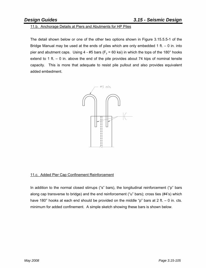
Design Guides 3.15 - Seismic Design
May 2008 Page 3.15-105
11.b. Anchorage Details at Piers and Abutments for HP Piles
The detail shown below or one of the other two options shown in Figure 3.15.5.5-1 of the
Bridge Manual may be used at the ends of piles which are only embedded 1 ft. – 0 in. into
pier and abutment caps. Using 4 - #5 bars (Fy = 60 ksi) in which the tops of the 180° hooks
extend to 1 ft. – 0 in. above the end of the pile provides about 74 kips of nominal tensile
capacity. This is more that adequate to resist pile pullout and also provides equivalent
added embedment.
11.c. Added Pier Cap Confinement Reinforcement
In addition to the normal closed stirrups (“s” bars), the longitudinal reinforcement (“p” bars
along cap transverse to bridge) and the end reinforcement (“u” bars); cross ties (#4’s) which
have 180° hooks at each end should be provided on the middle “p” bars at 2 ft. – 0 in. cts.
minimum for added confinement. A simple sketch showing these bars is shown below.

Design Guides 3.15 - Seismic Design
Page 3.15-106 May 2008
#4 Cross Tie
Middle “p” Bar
Pier Cap
#4 Cross Tie
Middle “p” Bar
Pier Cap
12. Dowel Bar Connection of Beams to Pier and Abutment Caps
As discussed in the introduction to the current example bridge, the connection between PPC
deck beams and substructures has historically been strong or not fuse like which is not optimal
according to the philosophy of IDOT’s ERS strategy. Two 1 in. φ dowel rods have traditionally
been used for the connection. It is desirable to make these connections somewhat weaker
(more fuse like) without potentially compromising the integrity of these connections for other
structural and service conditions these bridges may experience during their lifetime. As such,
the two dowel rods at each end of a beam (or an equivalent) should be designed to resist a
shear force equal to the lesser of 0.4 or Csm (the design acceleration coefficient) times the
tributary dead weight of beams plus overlay. For other classes of bridges in Illinois, the fraction
of dead weight used for this design load is 0.2. In addition, connection rods should not be less
than ¾ in. in diameter with a minimum yield strength of 36 ksi (tensile strength of 58 ksi). Note
that these provisions also apply for the design of the connections in single span PPC deck
beam bridges.
The shear strength of connection rods (or bars) should be calculated according to the equation
below with a φ factor of 1.0. The same equation for shear strength is used in Section 3.7.3 of
the Bridge Manual but with a φ factor of 0.75. It is from LRFD Article 6.13.2.12.
φRn = φ0.48AbFu (Eq. 6.13.2.12-1)

Design Guides 3.15 - Seismic Design
May 2008 Page 3.15-107
Where:
φ = 1.0
Ab = area of dowel rod (in.2)
Fu = tensile strength of rod (ksi)
Maximum Design Shear Force for Anchor Rods:
Use 0.39 (< 0.4) times tributary dead weight flowing into ends of 60 ft. span beams as
the governing design shear.
( )( )rods2
ksf 0.05 ft. 4 k/ft. 864.0ft. 6039.0R 21
u×+×
×= = 6.2 kips/rod
Allowable Shear per Rod:
Compute strengths of ¾ in. φ Grade 36 and Grade 55 rods.
φRn = φ0.48AbFu
φ = 1.0
Ab = 0.44 in.2
Fu = 58 and 75 ksi
φRn = φ0.48AbFu = (1.0)(0.48)(0.44)(58) = 12.2 kips (Grade 36)
φRn = φ0.48AbFu = (1.0)(0.48)(0.44)(75) = 15.8 kips (Grade 55)
Therefore, ¾ in. φ dowels of Grade 36 or Grade 55 are adequate (#6 rebar, Fy = 60 ksi, may
also be substituted).
13. Minimum Support Length (Seat Width) Requirements at Piers and Abutments
At a minimum, adequate seat widths shall be provided in the longitudinal direction only at piers
and abutments according to LRFD Article 4.7.4.4. The requirements of the LRFD Code are
generally not as stringent as those detailed in Section 3.15.4.2 of the Bridge Manual, and are

Design Guides 3.15 - Seismic Design
Page 3.15-108 May 2008
permitted for single and multi-span simply supported PPC deck beam bridges designed
according to the flexible option outlined in Section 3.15.8 of the Bridge Manual.
For bridges in Zone 2, the minimum required seat width at piers and abutments shall be
calculated as 150% of the following equation from the LRFD Code.
( )( ) in. S000125.01H08.0L02.08N 2+++= (Eq. 4.7.4.4-1)
Where:
L = total length of bridge for single or multi-span PPC deck beam
bridges (ft.)
H = average height of piers for multi-span PPC deck beam
bridges and taken a zero (0.0) for single span bridges (ft.)
S = bridge skew (°)
L is taken as the total length of the bridge due to the close proximity of the beam ends at piers
(i.e. they will easily push against each other if the anchor rods fuse). Since PPC deck beams
are already “wide” (3 ft. or 4 ft.), the transverse seat width requirements have been waived for
these bridges (but they are required, over and above that specified by the LRFD Code, for most
structures on the State System as outlined in Section 3.15.4.2 of the Bridge Manaul).
Minimum Required Support Length:
( )( ) in. S000125.01H08.0L02.08N 2+++=
L = 140 ft.
H = 10 ft.
S = 0°
( )( )
Length Support Req. Min. in. 17.41.5N andin. 6.110000125.011008.014002.08N 2
==×+×+×+=∴

Design Guides 3.15 - Seismic Design
May 2008 Page 3.15-109
Provided Support Length at Abutments:
13.5 in.7 in.
20.5 in.
13.5 in.7 in.
20.5 in.
Provided Support Length at Piers:
21 in.21 in.
42 in.
21 in.21 in.
42 in.
Therefore, provided support lengths at abutments and pier are adequate.
20.5 in. > 17.4 in. and 21 in. > 17.4 in. OK
Design Guides 3.15 - Seismic Design
Page 3.15-110 May 2008
14. Overview of Example Bridge Design With Metal Shell Piles
If the piles for the current example bridge were metal shell (MS) and not HP type; the design
steps, procedures and calculations would be quite similar to those presented in Parts 1 through
13 above. However, there are also some important differences. Given below is an abbreviated
design for the current example bridge with metal shell piles. Emphasized are the differences in
design procedures, etc. when metal shell piles are employed instead of HP piles.
14.a. Determination of Bridge Periods and Base Shears – Transverse and Longitudinal
Directions
The MS piles to be used for the example bridge are 14 in. x 0.25 in. (Fy = 45 ksi, f’c = 3.5 ksi
assumed for design). As shown in the calculations above, the HP piles did not significantly
contribute to the “seismic weight” of the bridge. It is assumed here that the MS piles do not
either. As such, 1220 kips will again be used as the mass (weight) of the bridge for seismic
design.
The transverse and longitudinal periods of the example bridge with MS piles can be
calculated in nearly the same manner as when the piles are HP. The primary difference is in
the stiffness calculation for the piles (and primarily involves the moment of inertia and/or the
modulus of elasticity). Other than this, Parts 1.b. through 1.f. for determining the transverse
period, etc., Parts 2.b. through 2.d. for determining the longitudinal period, etc., and the
methods for determining and distributing total seismic base design shears to the abutments
and piers in Part 3 are the same as outlined above.
It should be assumed that MS piles are reinforced concrete columns in soil with the shell
acting as both the longitudinal (vertical) and transverse (“spiral”) reinforcement. MS piles
may also have added spirals and longitudinal bars, but this scenario is not considered in the
current example. For typical or regular bridges, it is recommended that the stiffness of the
piles at the piers and abutments should be determined using the “equivalent” moments of
inertia, Ip, given in Appendix C for MS piles (even if there are added longitudinal bars
considered) and the modulus of elasticity for steel, Es (29000 ksi), as shown in the basic
equation for pier and abutment stiffnesses below.

Design Guides 3.15 - Seismic Design
May 2008 Page 3.15-111
height pileh where; h
IE3) or 12(piles) of .no(k p3
p
ps Abutor Pier =
××=
Alternatively, the pile moment of inertia may be computed based upon the steel only with the
equation below. In this case, Es should be substituted with Ee (an equivalent modulus of
elasticity using Eq. 6.9.5.1-5 of the LRFD Code), and Ip should be substituted with Ips in the
equation above.
shell pile of thicknesst
and diameter, pile gross where; 4
t2-
42
I
w
pile
4
wpile
4pile
ps
=
=φ⎟⎠⎞
⎜⎝⎛ −φπ⎟
⎠⎞
⎜⎝⎛φπ
=
The values for hp are determined in the same manner as for HP piles (see also Appendix C).
The fixed-fixed case should be used for the transverse direction (with the 12 factor) and the
fixed-pinned case should be used for the longitudinal direction (with the 3 factor). In the
longitudinal direction, the “softening” effects due to rigid body rotation of caps at piers and
abutments should be taken account of in the same manner as for HP piles.
Using depths-of-fixity from Appendix C (fixed-fixed depth = 9.1 ft., and fixed-pinned depth =
2 x 4.5 ft = 9.0 ft.), a modulus of elasticity of steel equal to 29000 ksi, and an equivalent
moment of inertia of 358.4 in.4, the following pier and abutment stiffnesses were obtained:
kPier(Trans) = 146.7 k/in.
kAbut(Trans) = 478.9 k/in.
kPier(Long) = 29.9 k/in.
kAbut(Long) = 87.4 k/in.
The transverse period was calculated to be 0.55 sec. using the simplified method and the
longitudinal period was determined to be 0.73 sec. As can be observed, the example bridge
with metal shell piles is stiffer in the transverse and longitudinal directions than when the
piles were HP. As such, the total base shears in the transverse and longitudinal directions
will be greater for the current example structure when MS piles are used. The following are
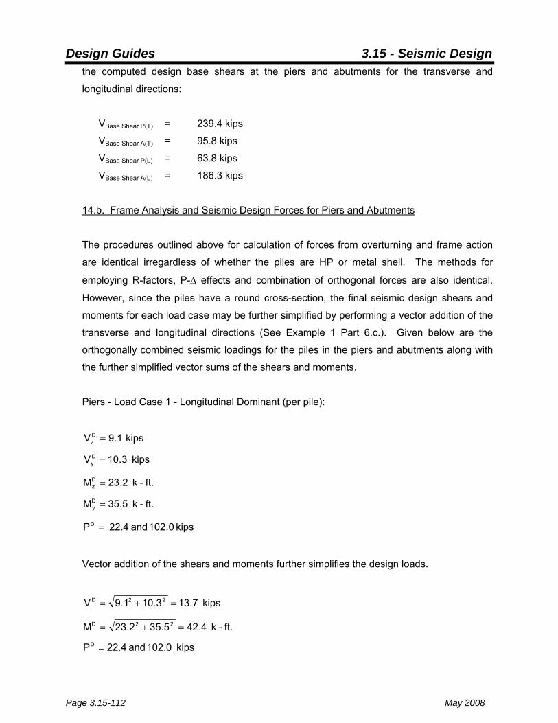
Design Guides 3.15 - Seismic Design
Page 3.15-112 May 2008
the computed design base shears at the piers and abutments for the transverse and
longitudinal directions:
VBase Shear P(T) = 239.4 kips
VBase Shear A(T) = 95.8 kips
VBase Shear P(L) = 63.8 kips
VBase Shear A(L) = 186.3 kips
14.b. Frame Analysis and Seismic Design Forces for Piers and Abutments
The procedures outlined above for calculation of forces from overturning and frame action
are identical irregardless of whether the piles are HP or metal shell. The methods for
employing R-factors, P-Δ effects and combination of orthogonal forces are also identical.
However, since the piles have a round cross-section, the final seismic design shears and
moments for each load case may be further simplified by performing a vector addition of the
transverse and longitudinal directions (See Example 1 Part 6.c.). Given below are the
orthogonally combined seismic loadings for the piles in the piers and abutments along with
the further simplified vector sums of the shears and moments.
Piers - Load Case 1 - Longitudinal Dominant (per pile):
kips 9.1V Dz =
kips 3.10VDy =
ft.-k 2.23MDz =
ft.-k 5.35MDy =
kips 0.102 and 22.4 PD =
Vector addition of the shears and moments further simplifies the design loads.
kips 7.133.101.9V 22D =+=
ft.-k 4.425.352.23M 22D =+=
kips 102.0 and 4.22PD =

Design Guides 3.15 - Seismic Design
May 2008 Page 3.15-113
Piers - Load Case 2 - Transverse Dominant (per pile):
kips 2.7VDz =
kips 2.34VDy =
ft.-k 5.77MDz =
ft.-k 6.10MDy =
kips 8.194 and (Ten.) 4.70 PD −=
Vector addition of the shears and moments further simplifies the design loads.
kips 3.342.347.2V 22D =+=
ft.-k 2.786.105.77M 22D =+=
kips 194.8 and (Ten.) 4.70PD −=
Abutments - Load Case 1 - Longitudinal Dominant (per pile):
kips 37.3VDz =
kips 8.5VDy =
ft.-k 5.17MDz =
ft.-k 1.174MDy =
kips 3.46 and 5.23 PD =
Vector addition of the shears and moments further simplifies the design loads.
kips 7.378.53.37V 22D =+=
ft.-k 0.1751.1745.17M 22D =+=
kips 46.3 and 5.23PD =

Design Guides 3.15 - Seismic Design
Page 3.15-114 May 2008
Abutments - Load Case 2 - Transverse Dominant (per pile):
kips 11.2VDz =
kips 2.19VDy =
ft.-k 3.58MDz =
ft.-k 2.52MDy =
kips 9.72 and (Ten.) 1.3 PD −=
Vector addition of the shears and moments further simplifies the design loads.
kips 2.222.192.11V 22D =+=
ft.-k 3.782.523.58M 22D =+=
kips 72.9 and (Ten.) 1.3PD −=
14.c. Combined Axial Force and Bending Structural Capacity Check for Piers and
Abutments
Appendix C provides nominal axial force - moment interaction strength diagrams for metal
shell piles which do not have added vertical or spiral reinforcement. The diagrams use a φ
factor of 1.0 as permitted in the IDOT ERS strategy and are suitable for design. They were
developed using standard methods of structural engineering with the metal shell considered
the columnar reinforcement according to LRFD Article 5.13.4.5.2. The axial force-moment
interaction diagram for MS 14 in. x 0.25 in. piles is shown below. The critical load case for
both the piers and abutments (Abutments – Load Case 1) is also superimposed on the
diagram. As can be observed, the loading is within the permissible envelope.

Design Guides 3.15 - Seismic Design
May 2008 Page 3.15-115
14.d. Pile Shear Structural Capacity Check, Minimum Steel, and Pile Connection Details
Seismic provisions for metal shell piles in Zone 2 are outlined in LRFD Article 5.13.4.6.2.
Provisions for Zones 3 and 4 are given in LRFD Article 5.13.4.6.3. As indicated in Part 14.c.
above, the metal shell is permitted to be considered as reinforcement. For many situations
in Zone 2 (and Zone 1), added reinforcement bars in the piles may not be required for multi-
span (or single span) simply supported PPC deck beam bridges designed using the flexible
option except for anchorage bars which are required when the piles are not embedded a full
2 ft. – 0 in. into caps at piers and abutments.
The cross sectional area of steel for 14 in. x 0.25 in. metal shells used in the current
example is 10.8 in.2. This is equivalent to almost 35 - #5 bars. So, the “reinforcement”
provided by these piles is substantial. The vertical steel ratio, ρ, based upon the gross area
of the piles (14 in. φ) is,
0702.0in. 7
in. 8.1022
2
=×π
=ρ

Design Guides 3.15 - Seismic Design
Page 3.15-116 May 2008
LRFD Article 5.13.4.6.2a requires pile anchorage to have a minimum steel ratio of 0.01
which equates to,
( ) 222a in. 54.1in. 701.0A =×π=
or about 5 - #5 bars. A modified version of the detail for metal shell reinforcement at
abutments given on Departmental Base Sheet F-MS may be used as an anchorage detail
when pile embedment at piers or abutments is only 1 ft. – 0 in. The detail calls for 6 - # 5
bars which are hooked 90° just above the end of the pile. The Base Sheet detail should be
modified using the detail shown in Part 11.b. above (or Bridge Manual Figure 3.15.5.5-1
Option B) as a guide. The bars should extend 1 ft. – 0 in. above the pile and be hooked
180°. When metal shell piles are embedded 2 ft. – 0 in., no added anchorage (connection)
reinforcement is typically needed except as required by design. See also Appendix C and
Section 3.15.5.5 of the Bridge Manual for further guidance. By inspection, uplift (tension) is
not a concern for the bridge in the current example (the nominal capacity of 6 - #5 bars is ≈
110 kips).
Minimum vertical (longitudinal) and spiral reinforcement requirements are outlined in LRFD
Article 5.13.4.6.2b. The minimum vertical steel reinforcement ratio is 0.005 which is
satisfied by inspection from the calculation of ρ above (0.0702). The spiral reinforcement
ratio provided by the metal shell may be calculated as follows,
0755.0.in75.61
in. 8.10 shell of height in. 1 a in concrete of Volume
shell of height in. 1 a in steel of Volume32
3
)Provided(s =×π×
==ρ
Article 5.13.4.6.2b requires a #3 spiral at 4 in. within the upper plastic hinging region which
equates to a spiral reinforcement ratio of (with the “spiral diameter” equal to 14 in. – 0.25 in.
= 13.75 in.),
0.0083475.675.1311.0
turn spiral 1 in concrete of Volumeturn spiral 1 of Volume
2s =××π
×π×==ρ

Design Guides 3.15 - Seismic Design
May 2008 Page 3.15-117
Therefore, the shell provides just over 9 times the minimum required steel and is adequate
for confinement. A cursory check of the shear strength provided by the shell (see the
method presented in Example 1 Part 7.b.) in comparison to the design shears also shows
ample adequacy.
14.e. Pier Cap Reinforcement, Connection of Beams to Pier and Abutment Caps, and
Support Lengths
Pier caps should have the same added reinforcement described in Part 11.c above. The
dowel bar connection should be designed according to Part 12, and support lengths should
be verified according to Part 13.

Design Guides 3.15 - Seismic Design
Page 3.15-118 May 2008

Design Guides 3.15 - Seismic Design
May 2008 Page 3.15-119
Appendix A: Columnar Axial Force Solutions due to Overturning Moment for 12 Cases

Design Guides 3.15 - Seismic Design
Page 3.15-120 May 2008
Sp
d
PSTarm
dMP
dPMarmSM
ST
ST
p
=∴
×=
×=
PST
Sp
d
PSTarm
dMP
dPMarmSM
ST
ST
p
=∴
×=
×=
PST
Case A.1: Overturning Axial Forces for 2 Column Piers or 2 Piles in a Row
Sp
d d
PST0
arm
d2MP
d2PMarmSM
ST
ST
p
=∴
×=
×=
PST
Sp
d d
PST0
arm
d2MP
d2PMarmSM
ST
ST
p
=∴
×=
×=
PST
Case A.2: Overturning Axial Forces for 3 Column Piers or 3 Piles in a Row

Design Guides 3.15 - Seismic Design
May 2008 Page 3.15-121
Sp
d d
PSTarm0.33PST
d
PST
0.33PST
( )( )
dM
103P
dP2 dP2M
armSM
ST
21
ST31
23
ST
p
=∴
×
+×=
×=
Sp
d d
PSTarm0.33PST
d
PST
0.33PST
( )( )
dM
103P
dP2 dP2M
armSM
ST
21
ST31
23
ST
p
=∴
×
+×=
×=
Case A.3: Overturning Axial Forces for 4 Column Piers or 4 Piles in a Row
Sp
d
PSTarm0.5PST
PST
0.5PST
( )( )
dM
51P
dP2 d2P2M
armSM
ST
ST21ST
p
=∴
×
+×=
×=
d d d
0
Sp
d
PSTarm0.5PST
PST
0.5PST
( )( )
dM
51P
dP2 d2P2M
armSM
ST
ST21ST
p
=∴
×
+×=
×=
d d d
0
Case A.4: Overturning Axial Forces for 5 Column Piers or 5 Piles in a Row
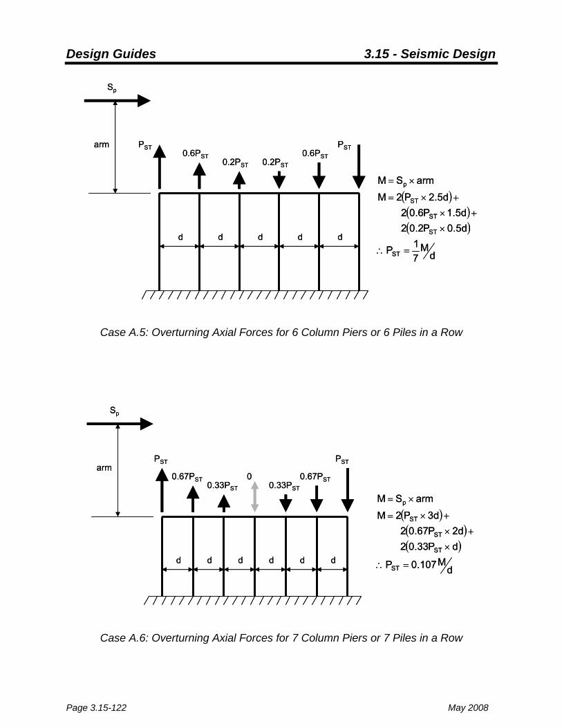
Design Guides 3.15 - Seismic Design
Page 3.15-122 May 2008
Sp
d
PSTarm0.6PST
PST0.6PST
( )( )( )
dM
71P
d5.0P2.02 d5.1P6.02
d5.2P2MarmSM
ST
ST
ST
ST
p
=∴
×
+×
+×=
×=
d d d d
0.2PST0.2PST
Sp
d
PSTarm0.6PST
PST0.6PST
( )( )( )
dM
71P
d5.0P2.02 d5.1P6.02
d5.2P2MarmSM
ST
ST
ST
ST
p
=∴
×
+×
+×=
×=
d d d d
0.2PST0.2PST
Case A.5: Overturning Axial Forces for 6 Column Piers or 6 Piles in a Row
Sp
d
PSTarm
0.67PST
PST
0.67PST
( )( )( )
dM107.0P
dP33.02 d2P67.02
d3P2MarmSM
ST
ST
ST
ST
p
=∴
×
+×
+×=
×=0.33PST0.33PST
0
d d d d d
Sp
d
PSTarm
0.67PST
PST
0.67PST
( )( )( )
dM107.0P
dP33.02 d2P67.02
d3P2MarmSM
ST
ST
ST
ST
p
=∴
×
+×
+×=
×=0.33PST0.33PST
0
d d d d d
Case A.6: Overturning Axial Forces for 7 Column Piers or 7 Piles in a Row

Design Guides 3.15 - Seismic Design
May 2008 Page 3.15-123
Sp
d
arm0.71PST
PST
( )( )( )( )
dM083.0d
M121P
d5.0P14.02 d5.1P43.02 d5.2P71.02
d5.3P2MarmSM
ST
ST
ST
ST
ST
p
==∴
×
+×
+×
+×=
×=0.43PST
0.14PST
d d d d d d
Sp
d
arm0.71PST
PST
( )( )( )( )
dM083.0d
M121P
d5.0P14.02 d5.1P43.02 d5.2P71.02
d5.3P2MarmSM
ST
ST
ST
ST
ST
p
==∴
×
+×
+×
+×=
×=0.43PST
0.14PST
d d d d d d
Case A.7: Overturning Axial Forces for 8 Column Piers or 8 Piles in a Row
Sp
d
arm0.75PST
PST
( )( )( )( )
dM067.0d
M151P
dP25.02 d2P5.02
d3P75.02 d4P2M
armSM
ST
ST
ST
ST
ST
p
==∴
×
+×
+×
+×=
×=0.5PST
0.25PST0
d d d d d d d
Sp
d
arm0.75PST
PST
( )( )( )( )
dM067.0d
M151P
dP25.02 d2P5.02
d3P75.02 d4P2M
armSM
ST
ST
ST
ST
ST
p
==∴
×
+×
+×
+×=
×=0.5PST
0.25PST0
d d d d d d d
Case A.8: Overturning Axial Forces for 9 Column Piers or 9 Piles in a Row
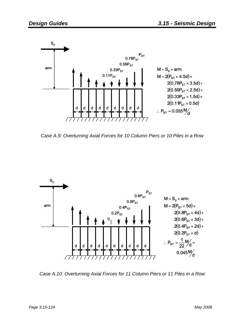
Design Guides 3.15 - Seismic Design
Page 3.15-124 May 2008
Sp
d
arm
0.78PST
PST
( )( )( )( )( )
dM055.0P
d5.0P11.02 d5.1P33.02 d5.2P56.02 d5.3P78.02
d5.4P2MarmSM
ST
ST
ST
ST
ST
ST
p
=∴
×
+×
+×
+×
+×=
×=0.56PST
0.11PST
d d d d d d d d
0.33PST
Sp
d
arm
0.78PST
PST
( )( )( )( )( )
dM055.0P
d5.0P11.02 d5.1P33.02 d5.2P56.02 d5.3P78.02
d5.4P2MarmSM
ST
ST
ST
ST
ST
ST
p
=∴
×
+×
+×
+×
+×=
×=0.56PST
0.11PST
d d d d d d d d
0.33PST
Case A.9: Overturning Axial Forces for 10 Column Piers or 10 Piles in a Row
Sp
d
arm
0.8PST
PST
( )( )( )( )( )
dM045.0
dM
221P
dP2.02 d2P4.02 d3P6.02 d4P8.02
d5P2MarmSM
ST
ST
ST
ST
ST
ST
p
==∴
×
+×
+×
+×
+×=
×=0.6PST
0.2PST
d d d d d d d d
0.4PST
0
d
Sp
d
arm
0.8PST
PST
( )( )( )( )( )
dM045.0
dM
221P
dP2.02 d2P4.02 d3P6.02 d4P8.02
d5P2MarmSM
ST
ST
ST
ST
ST
ST
p
==∴
×
+×
+×
+×
+×=
×=0.6PST
0.2PST
d d d d d d d d
0.4PST
0
d
Case A.10: Overturning Axial Forces for 11 Column Piers or 11 Piles in a Row

Design Guides 3.15 - Seismic Design
May 2008 Page 3.15-125
Sp
d
arm
d d d d d d d d d d
0.82PST
0.64PST
0.27PST
0.46PST
0.09PST
PST
( )( )( )( )( )( )
dM038.0
dM
261P
d5.0P09.02 d5.1P27.02 d5.2P46.02 d5.3P64.02 d5.4P82.02
d5.5P2MarmSM
ST
ST
ST
ST
ST
ST
ST
p
==∴
×
+×
+×
+×
+×
+×=
×=
Sp
d
arm
d d d d d d d d d d
0.82PST
0.64PST
0.27PST
0.46PST
0.09PST
PST
( )( )( )( )( )( )
dM038.0
dM
261P
d5.0P09.02 d5.1P27.02 d5.2P46.02 d5.3P64.02 d5.4P82.02
d5.5P2MarmSM
ST
ST
ST
ST
ST
ST
ST
p
==∴
×
+×
+×
+×
+×
+×=
×=
Case A.11: Overturning Axial Forces for 12 Column Piers or 12 Piles in a Row
Sp
d
arm
0.83PST
PST
0.67PST
0.33PST
d d d d d d d d
0.5PST
d d d
0.17PST0
( )( )( )( )( )( )
dM033.0P
dP17.02 d2P33.02
d3P5.02 d4P67.02 d5P83.02
d6P2MarmSM
ST
ST
ST
ST
ST
ST
ST
p
=∴
×
+×
+×
+×
+×
+×=
×=
Sp
d
arm
0.83PST
PST
0.67PST
0.33PST
d d d d d d d d
0.5PST
d d d
0.17PST0
( )( )( )( )( )( )
dM033.0P
dP17.02 d2P33.02
d3P5.02 d4P67.02 d5P83.02
d6P2MarmSM
ST
ST
ST
ST
ST
ST
ST
p
=∴
×
+×
+×
+×
+×
+×=
×=
Case A.12: Overturning Axial Forces for 13 Column Piers or 13 Piles in a Row

Design Guides 3.15 - Seismic Design
Page 3.15-126 May 2008

Design Guides 3.15 - Seismic Design
May 2008 Page 3.15-127
Appendix B: Columnar Axial Force Solutions due to Frame Action for 5 Cases

Design Guides 3.15 - Seismic Design
Page 3.15-128 May 2008
d
col. right Comp. & col. left Tension P
dM2
dMMP
VPMM
SB
STSTSTSB
SBSB
STSB
=
±=+
=
=
=
VST VST
MST
h
MSB
VSB
VSB
PSB
d
Note: VST not shown for clarity
2SV P
ST =
d
col. right Comp. & col. left Tension P
dM2
dMMP
VPMM
SB
STSTSTSB
SBSB
STSB
=
±=+
=
=
=
VST VST
MST
h
MSB
VSB
VSB
PSB
d
Note: VST not shown for clarity
2SV P
ST =
Case B.1: Frame Action Axial Forces for 2 Column Piers or 2 Piles in a Row

Design Guides 3.15 - Seismic Design
May 2008 Page 3.15-129
d
col. right Comp. & center, zero col., left Tension P
dM5.1
d2
MMP
VPMM
SB
STST
STSB
SBSB
STSB
=
±=+
=
=
=
VST VST VST
MST
h
MSB MSB/2VSB
VSB
PSB
d
Note: VST not shown for clarity
3SV P
ST =
d
col. right Comp. & center, zero col., left Tension P
dM5.1
d2
MMP
VPMM
SB
STST
STSB
SBSB
STSB
=
±=+
=
=
=
VST VST VST
MST
h
MSB MSB/2VSB
VSB
PSB
d
Note: VST not shown for clarity
3SV P
ST =
Case B.2: Frame Action Axial Forces for 3 Column Piers or 3 Piles in a Row

Design Guides 3.15 - Seismic Design
Page 3.15-130 May 2008
d
col. right far Comp. & & col. left far Tension P
dM67.1
d3
M2MP
VP ;MM
SB
STST
STSB
SBSBSTSB
=
±=+
=
==
VST VST VST
MST
h
MSB 2MSB/3
VSB
VSB
PSB
d
Note: VST not shown for clarity
4SV P
ST =
VST
2MSB/3 MSB/3
0.4VSB
VSB
d
MST
0.6PSB
MSB/3
0.4VSB
d
col. right far Comp. & & col. left far Tension P
dM67.1
d3
M2MP
VP ;MM
SB
STST
STSB
SBSBSTSB
=
±=+
=
==
VST VST VST
MST
h
MSB 2MSB/3
VSB
VSB
PSB
d
Note: VST not shown for clarity
4SV P
ST =
VST
2MSB/3 MSB/3
0.4VSB
VSB
d
MST
0.6PSB
MSB/3
0.4VSB
Case B.3: Frame Action Axial Forces for 4 Column Piers or 4 Piles in a Row

Design Guides 3.15 - Seismic Design
May 2008 Page 3.15-131
d
col. right far Comp. & & col. left far Tension P
dM67.1
d3
M2MP
VP ;MM
SB
STST
STSB
SBSBSTSB
=
±=+
=
==
VST VST VST
MST
h
MSB2MSB/3
VSB
VSB
PSB
d
Note: VST not shown for clarity
5SV P
ST =
VST
2MSB/3 MSB/3
0.5VSB
VSB
d
MST
0.5PSB
MSB/2
0.5VSB
MSB/2 MSB/2
0.5VSB
0.5VSB
d
MST
0.0
0.5VSB
VST
MSB/3d
col. right far Comp. & & col. left far Tension P
dM67.1
d3
M2MP
VP ;MM
SB
STST
STSB
SBSBSTSB
=
±=+
=
==
VST VST VST
MST
h
MSB2MSB/3
VSB
VSB
PSB
d
Note: VST not shown for clarity
5SV P
ST =
VST
2MSB/3 MSB/3
0.5VSB
VSB
d
MST
0.5PSB
MSB/2
0.5VSB
MSB/2 MSB/2
0.5VSB
0.5VSB
d
MST
0.0
0.5VSB
VST
MSB/3
Case B.4: Frame Action Axial Forces for 5 Column Piers or 5 Piles in a Row

Design Guides 3.15 - Seismic Design
Page 3.15-132 May 2008
d
col. right far Comp. & & col. left far Tension P
dM67.1
d3
M2MP
VP ;MM
SB
STST
STSB
SBSBSTSB
=
±=+
=
==
VST VST VST
MST
h
MSB2MSB/3
VSB
VSB
PSB
d
Notes: 1.VST not shownfor clarity.
2. Fourth Column through (No. of Columns-3) have zero axial force.
( )6 than greater whencolumns of no.by divided or 6SV P
ST =
VST
2MSB/3 MSB/3
0.5VSB
VSB
d
MST
0.5PSB
MSB/2
0.5VSB
MSB/2 MSB/2
0.6VSB
0.5VSB
d
MST
0.6VSB
VST
MSB/2
VST
0.1PSB
d
col. right far Comp. & & col. left far Tension P
dM67.1
d3
M2MP
VP ;MM
SB
STST
STSB
SBSBSTSB
=
±=+
=
==
VST VST VST
MST
h
MSB2MSB/3
VSB
VSB
PSB
d
Notes: 1.VST not shownfor clarity.
2. Fourth Column through (No. of Columns-3) have zero axial force.
( )6 than greater whencolumns of no.by divided or 6SV P
ST =
VST
2MSB/3 MSB/3
0.5VSB
VSB
d
MST
0.5PSB
MSB/2
0.5VSB
MSB/2 MSB/2
0.6VSB
0.5VSB
d
MST
0.6VSB
VST
MSB/2
VST
0.1PSB
Case B.5: Frame Action Axial Forces for 6 or More Column Piers or 6 or More Piles in a
Row

Design Guides 3.15 - Seismic Design
May 2008 Page 3.15-133
Appendix C: Approximate Fixity Depths for H-Piles and Metal Shell Piles in Site Class
D Soil, and Axial Force-Moment Interaction Diagrams for Metal Shell Piles Fixity depths which are generally suitable for typical seismic design for a wide range of situations are given in Tables C.1 and C.2. Table C.1 presents depth-of-fixity values for steel H-piles and Table C.2 presents depths-of-fixity for Metal Shell (MS) piles. Three boundary conditions are given. These are fixed-fixed, fixed-pinned, and the average of the two conditions. For H-piles, values for both the weak and strong axes are provided. The provided moments of intertia for MS piles are “equivalent”. The shell and the concrete behave as a reinforced concrete column with the shell acting as the reinforcement. The provided moments of interia are at zero axial force and first yield of the steel shells under pure moment in soil. For all computed depths-of-fixity, the soil was assumed to have properties at the mid-point of Site Class D as defined in Appendix A of Section 3.15 of the Bridge Manual and in Section 3 of the LRFD Code. However, it should be noted that Site Class D soil was only assumed to be in the “local region” of the pile, or about 2 to 3 times a pile’s fixity depth (in terms of deflection), and not necessarily in the entire upper 100 ft. of the soil profile. The upper 100 ft. of the soil profile is typically used to determine the actual Site Class and corresponding Site Coefficients used to calculate the design response spectrum for a structure, but is not necessarily relevant for determination of pile fixity depths. Class D soil can fall into Soil Profile Types II or III as defined in LFD Div. I-A. The Soil Profile or Site Class Definitions in Appendix A of Section 3.15 of the Bridge Manual and the LRFD Code are much more descriptive and numerically specific than those in the LFD Specifications. The depths-of-fixity given in Tables C.1 and C.2 may be used for soils with properties ranging from the lower bounds of Site Class C to the upper bounds of Site Class E for typical or “regular” bridges in Illinois (see Section 3.15.3.2 of the Bridge Manual for more information). The upper bounds of Site Class C soils tend to approach the properties of rock and are very stiff. Pile foundations may not be applicable for such soils or piles may be set into rock (for which the depth-of-fixity would be known). The lower bounds of Site Class E tend to approach poor site conditions for which special geotechnical and structural considerations are necessary. Some engineering judgment concerning the use of Tables C.1 and C.2 is required for borderline cases.

Design Guides 3.15 - Seismic Design
Page 3.15-134 May 2008
The depths-of-fixity given in Tables C.1 and C.2 are primarily intended for seismic design. Engineering judgment is required when using these tables for non-extreme event loadings. Lateral load versus deflection curves (that are non-linear) were generated for each considered case up to structural deformations which were just past initial yielding of the steel. Linear regression was used to fit straight lines to the generated curves. The slope of each fitted line represents a simplified stiffness (and depth-of-fixity) about the axes and for the boundary conditions considered for each pile. The structural stiffness of piles that are at or beyond initial yielding of the steel are “softer” than for non-extreme event loading conditions. For typical bridge designs, the fixed-fixed case for piles is appropriate for many situations if the guidelines given in Section 3.10 and 3.15 of the Bridge Manual are followed for seismic design. However, cases where fixed-pinned is appropriate are also common. The fixity depths given in Tables C.1 and C.2 are presented in terms of moment at initial yielding of the steel and not deflection. For the fixed-fixed boundary condition case, fixity depths based upon moment and deflection are typically similar. However, for the fixed-pinned case, fixity depths based upon deflection are typically about twice that of the depths based upon moment. When required for global analytical models of bridges, it is more accurate to calculate substructure/foundation stiffnesses with depths-of-fixity based upon deflection. For local analytical models, though, especially when used in conjunction with Appendix B, it is more accurate to calculate design forces with depths-of-fixity based upon moment. See Examples 1 and 4 for applications of these principles in conjunction with Tables C.1 and C.2. Figures C.1 through C.4 provide nominal axial strength vs. moment strength interaction curves for MS piles. These may be used for structural design of the piles as columns in soil and are not an indicator of geotechnical capacity. MS piles may also have supplemental longitudinal (vertical) and shear/confinement (spiral) reinforcement provided in order to increase structural moment, axial force, and/or shear capacity. Figures C.1 through C.4 are for MS piles without supplemental reinforcement. Note that, in general, the details for reinforcement provided inside of MS piles on the Departmental Base Sheet (F-MS) at abutments are not considered structural for resisting moment or axial force from seismic loadings and should not be considered for confinement or shear. The depth of vertical and spiral reinforcement shown on the Departmental Base Sheet for MS piles is typically insufficient for development of plastic hinges associated with seismic design principles. However, if piles are embedded at least 2 ft. – 0 in. into piers or abutments, the details may be considered as anchorage reinforcement without modification. The individual encasement detail for piles at piers on Base Sheet F-MS should

Design Guides 3.15 - Seismic Design
May 2008 Page 3.15-135
never be considered structural. See Section 3.15.5.5 of the Bridge Manual and Part 14 of Example 4 for additional guidance. The information on fixity depths given below may be used at the designer’s discretion. More complex analyses and refined stiffness determinations are not discouraged by the Department. When more accurate methods are used to determine pile fixity depths, the tables below can be used a guide to gauge whether a more sophisticated analysis is “in the ballpark”. The fixity depths presented in Tables C.1 and C.2 have been established for a variable range of soil conditions and design parameters intended to encompass a large population of structures. Given the variability that is likely to exist between a subject structure and the assumptions used in establishing the fixity depths, it is considered permissible to neglect “group action” factors when using the fixity depths presented in Tables C.1 and C.2.
Mom. of Inertia Fix-Fix Fix-Pin Average Mom. of Inertia Fix-Fix Fix-Pin AverageStrong Depth Depth Depth Weak Depth Depth DepthAxis of Fixity of Fixity of Fixity Axis of Fixity of Fixity of Fixity
Pile (in.4) (ft.) (ft.) (ft.) (in.4) (ft.) (ft.) (ft.)HP 14x117 1220 12.5 6.3 9.4 443 9.8 4.8 7.3HP 14x102 1050 12.0 6.1 9.1 380 9.3 4.6 7.0HP 14x89 904 11.6 5.8 8.7 326 8.9 4.4 6.7 HP 14x73 729 10.9 5.5 8.2 261 8.4 4.2 6.3 HP 12x84 650 10.9 5.5 8.2 213 8.3 4.1 6.2HP 12x74 569 10.5 5.3 7.9 186 8.0 4.0 6.0HP 12x63 472 10.0 5.1 7.6 153 7.7 3.8 5.7HP 12x53 393 9.6 4.9 7.2 127 7.3 3.6 5.5HP 10x57 294 9.3 4.7 7.0 101 7.2 3.6 5.4HP 10x42 210 8.6 4.4 6.5 71.7 6.7 3.3 5.0 HP 8x36 119 8.0 4.0 6.0 40.3 6.2 3.1 4.6
Table C.1: Fixity Depths in Site Class D Soil for H-Piles
Equiv. Fix-Fix Fix-Pin Average
Mom. of Inertia Depth Depth DepthAxis of Fixity of Fixity of Fixity
Pile (in.4) (ft.) (ft.) (ft.)MS 14x0.312 420 9.5 4.7 7.1MS 14x0.25 358.4 9.1 4.5 6.8MS 12x0.25 214.2 8.3 4.1 6.2MS 12x0.179 163.2 7.7 3.8 5.8
Table C.2: Fixity Depths in Site Class D Soil for Metal Shell Piles

Design Guides 3.15 - Seismic Design
Page 3.15-136 May 2008
Figure C.1: Nominal Axial Strength vs. Moment Strength Interaction Diagram for 12 x
0.179 in. Metal Shell Piles with Fy = 45 ksi and f’c = 3.5 ksi
Figure C.2: Nominal Axial Strength vs. Moment Strength Interaction Diagram for 12 x
0.25 in. Metal Shell Piles with Fy = 45 ksi and f’c = 3.5 ksi

Design Guides 3.15 - Seismic Design
May 2008 Page 3.15-137
Figure C.3: Nominal Axial Strength vs. Moment Strength Interaction Diagram for 14 x
0.25 in. Metal Shell Piles with Fy = 45 ksi and f’c = 3.5 ksi
Figure C.4: Nominal Axial Strength vs. Moment Strength Interaction Diagram for 14 x
0.312 in. Metal Shell Piles with Fy = 45 ksi and f’c = 3.5 ksi

Design Guides 3.15 - Seismic Design
Page 3.15-138 May 2008