3.11 adaptive data assimilation to include spatially variable observation error statistics rod...
TRANSCRIPT
3.11 Adaptive Data Assimilation to Include Spatially Variable Observation
Error Statistics
Rod FrehlichUniversity of Colorado, Boulder
andRAL/NCAR
Funded by NSF (Lydia Gates)
Turbulence
• Small scale turbulence defines the observation sampling error or “error of representativeness”
• Critical component of the total observation error
• Turbulence and observation sampling error have large spatial variations
• Optimal data assimilation must include these variations

Spatial Spectra
• Robust description in troposphere
• Power law scaling
• Spectral level defines turbulence (ε2/3 and CT
2)

Structure Functions
• Alternate spatial statistic
• Also has power law scaling
• Structure functions (and spectra) from model output are filtered
• Corrections are possible by comparisons with in situ data
• Produce local estimates of turbulence defined by ε or CT
2 for adaptive data assimilation

RUC20 Analysis
• RUC20 model structure function
• In situ “truth” from GASP data
• Effective spatial filter (3.5Δ) determined by agreement with theory
DEFINITION OF TRUTH
• For forecast error, truth is defined by the spatial filter of the model numerics
• For the initial field (analysis) truth should have the same definition for consistency

Observation Sampling Error
• Truth is the average of the variable x over the LxL effective grid cell
• Total observation error
• Instrument error = x
• Sampling error = x• The observation sampling pattern and
the local turbulence determines the sampling error
2 2 2x x xΣ = σ + δ
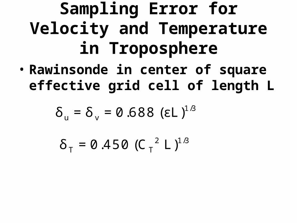
Sampling Error for Velocity and Temperature in Troposphere
• Rawinsonde in center of square effective grid cell of length L
1/3u vδ = δ = 0.688 (εL)
2 1/3T Tδ = 0.450 (C L)
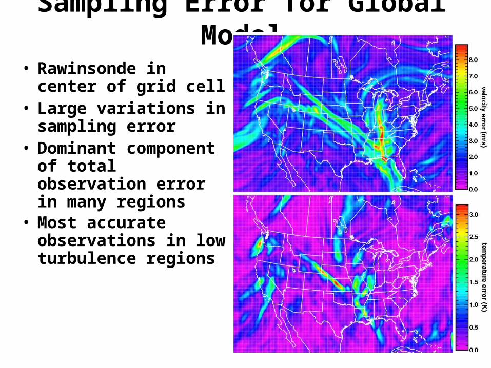
Sampling Error for Global Model
• Rawinsonde in center of grid cell
• Large variations in sampling error
• Dominant component of total observation error in many regions
• Most accurate observations in low turbulence regions
Optimal Data Assimilation
• Optimal assimilation requires estimation of total observation error covariance
• Requires calculation of instrument error which may depend on local turbulence (profiler, Doppler lidar)
• Requires calculation of sampling error • Calculation of analysis error
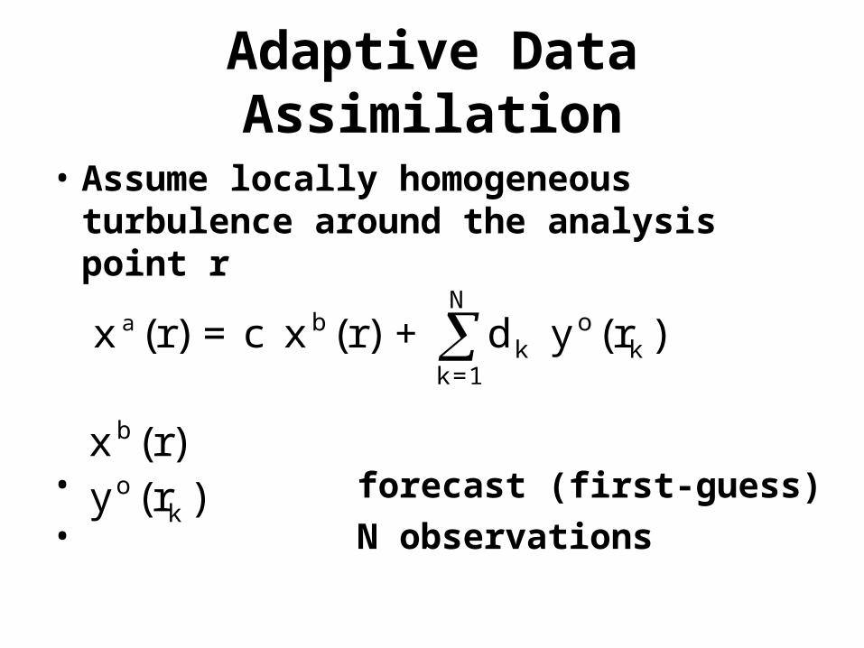
Adaptive Data Assimilation
• Assume locally homogeneous turbulence around the analysis point r
• forecast (first-guess)
• N observations
aN
b ok k
k=1
x (r) = c x (r) + d y (r )
oky (r )
bx (r)

Measurement Geometry
• Single observation at the analysis coordinate
• Multiple observations around the analysis coordinate
• Aircraft track
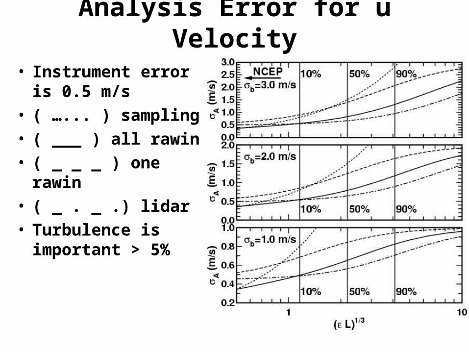
Analysis Error for u Velocity
• Instrument error is 0.5 m/s
• ( …... ) sampling• ( ___ ) all rawin• ( _ _ _ ) one rawin• ( _ . _ .) lidar• Turbulence is
important > 5%

SUMMARY
• Turbulence produces large spatial variations in total observation error
• Optimal data assimilation using local estimates of turbulence reduces the analysis error

NCAR Collaborators
• Bob Sharman
• Francois Vandenberghe
• Yubao Liu
• Josh Hacker
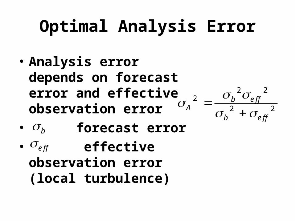
Optimal Analysis Error
• Analysis error depends on forecast error and effective observation error
• forecast error
• effective observation error (local turbulence)
2 22
2 2b eff
Ab eff
beff

Analysis Error for Temperature
• Instrument error is 0.5 K
• ( . . . . ) sampling error
• ( ___ ) all data• ( - - - ) single obs.• ( . - . - ) aircraft • Turbulence is
important > 50%
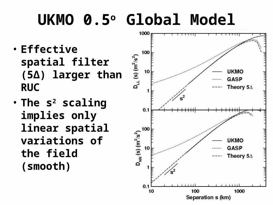
UKMO 0.5o Global Model
• Effective spatial filter (5Δ) larger than RUC
• The s2 scaling implies only linear spatial variations of the field (smooth)

GFS 0.5o Global Model
• Effective spatial filter (5Δ) is the same as UKMO

Estimates of Small Scale Turbulence
• Calculate structure functions locally over LxL square
• Determine best-fit to empirical model
• Estimate in situ turbulence level and ε
ε1/3
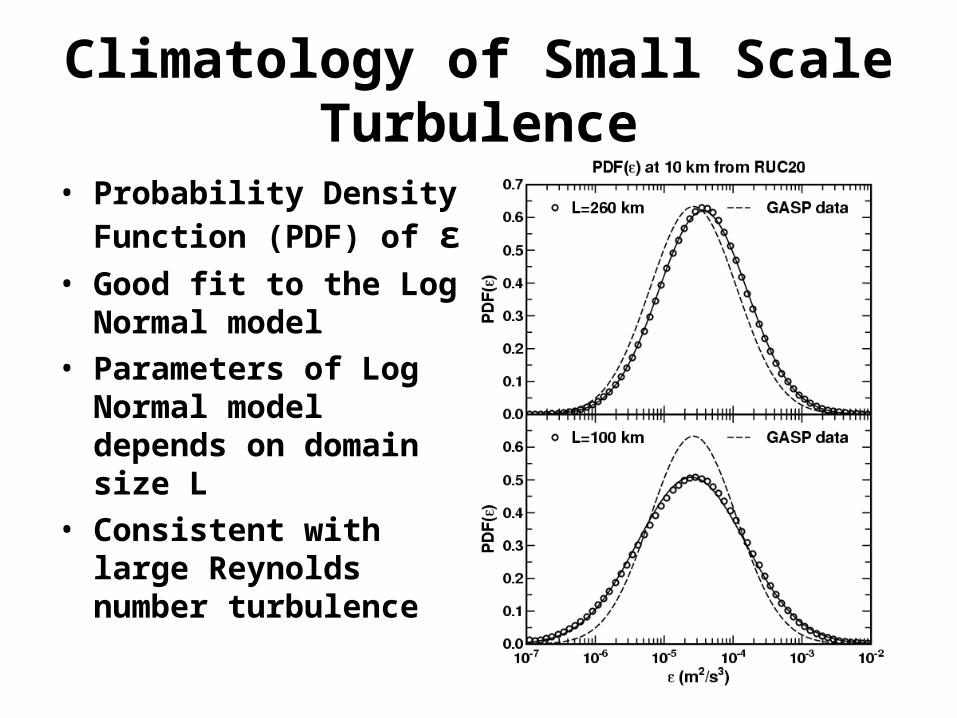
Climatology of Small Scale Turbulence
• Probability Density Function (PDF) of ε
• Good fit to the Log Normal model
• Parameters of Log Normal model depends on domain size L
• Consistent with large Reynolds number turbulence
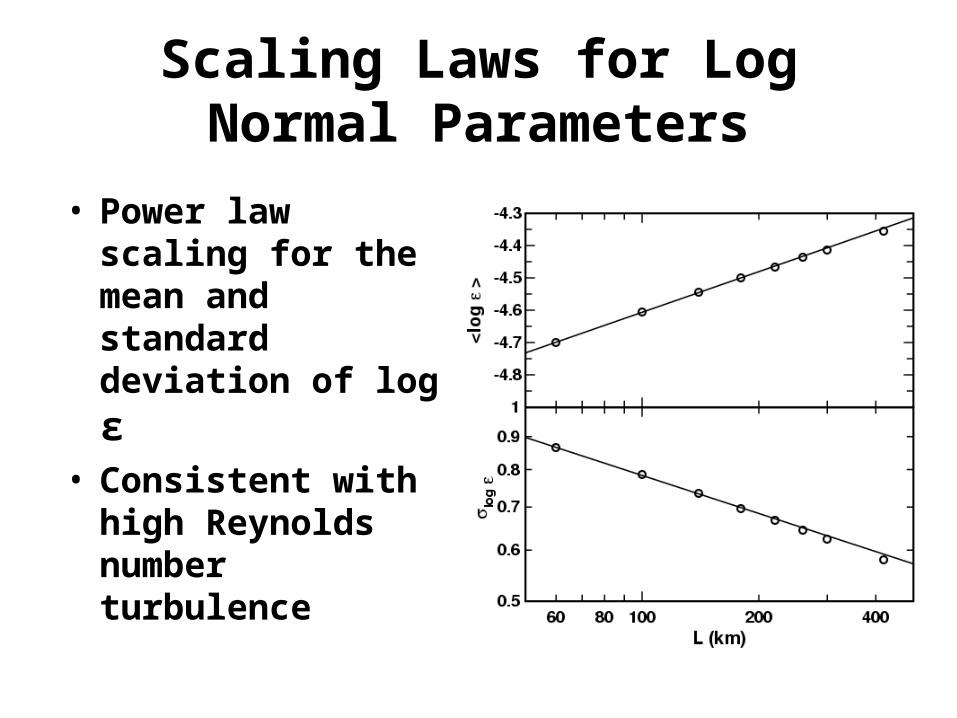
Scaling Laws for Log Normal Parameters
• Power law scaling for the mean and standard deviation of log ε
• Consistent with high Reynolds number turbulence