3. real business cycle theory - uni-leipzig.de · institut für theoretische volkswirtschaftslehre...

Institut für Theoretische VolkswirtschaftslehreMakroökonomik

Prof. Dr. Thomas StegerAdvanced Macroeconomics II | Lecture| SS 12Advanced Macroeconomics II | Lecture| SS 12

3. Real Business Cycle Theory

Introduction

Simplistic RBC Model

Si l t h ti th d l Simple stochastic growth model

Baseline RBC model


Real Business Cycle Theory

I t d ti (1)Introduction (1)

Business cycle research studies the causes and consequences of the recurrent expansions and contractions in aggregate economic activity that occur in most industrialized countries.and contractions in aggregate economic activity that occur in most industrialized countries.

Kydland and Prescott (1982) and Long and Plosser (1983) strikingly illustrated that one could build a successful business cycle model that involved market clearing, no monetary factors

d i l f i liand no rational for macroeconomic policy.

Simple equilibrium models, driven by shifts in TFP, could generate time series with the same complex patterns of persistence, comovement and volatility as those of actual economies.p p p , y

The models of the RBC research program are now widely applied in monetary economics, international economics, public finance, labor economics, and asset pricing. f h d l i i l di i l b i l k f il Many of these model economies, in contrast to early RBC studies, involve substantial market failures,

so that government intervention is desirable. In others, the business cycle is driven by monetary shocks or by exogenous shocks in beliefs. DSGE d l b th l b t i hi h d i l i i d t d DSGE models are by now the laboratory in which modern macroeconomic analysis is conducted.

There has been increasing concern about the mechanisms at the core of the standard RBC models: business cycles are driven mainly by large and cyclically volatile shocks to

2

productivity, which are well represented by Solow residuals.



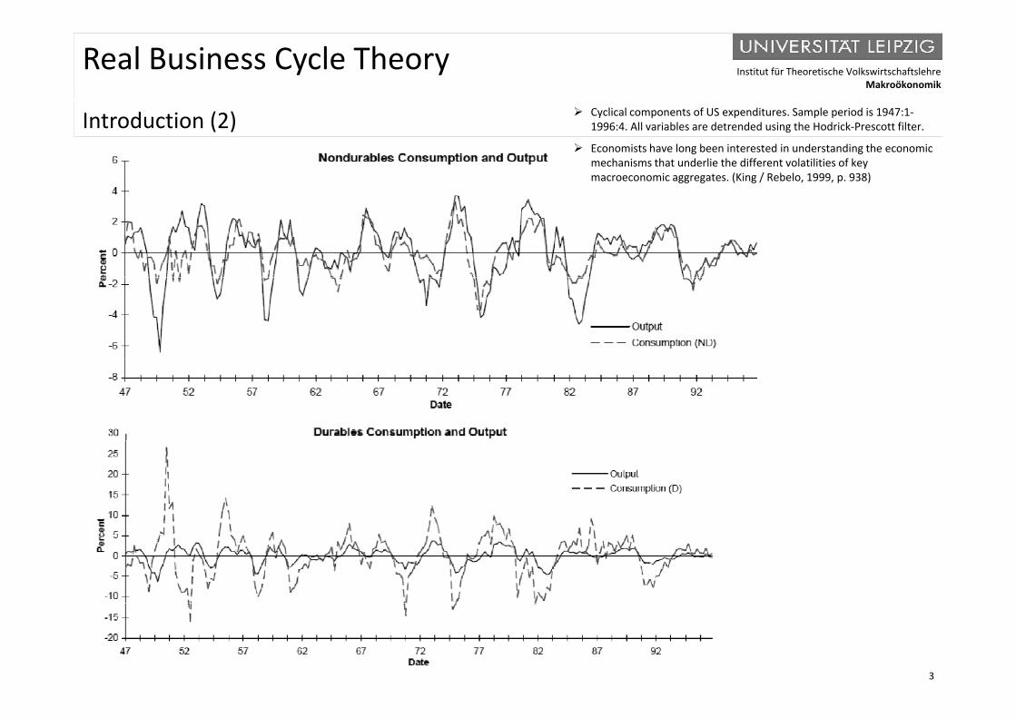
I t d ti (2) Cyclical components of US expenditures. Sample period is 1947:1-Introduction (2) Cyclical components of US expenditures. Sample period is 1947:11996:4. All variables are detrended using the Hodrick-Prescott filter.

Economists have long been interested in understanding the economic mechanisms that underlie the different volatilities of key macroeconomic aggregates. (King / Rebelo, 1999, p. 938)

3




4




5




6




7




8




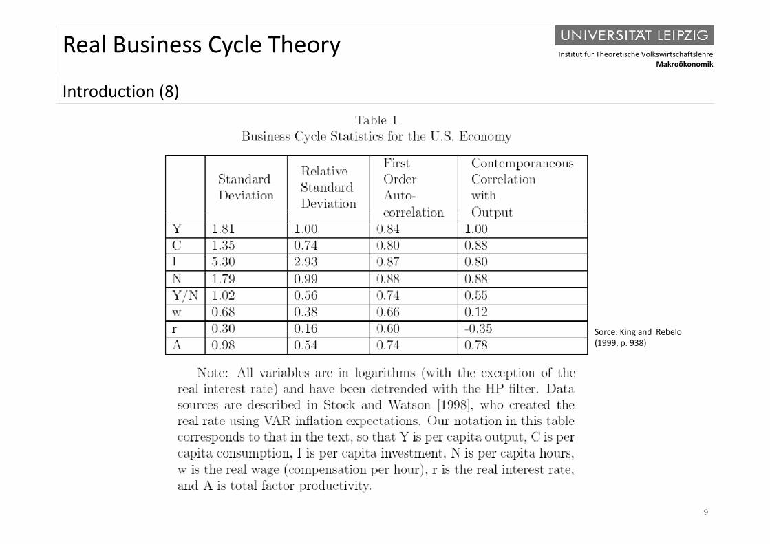
Sorce: King and RebeloSorce: King and Rebelo(1999, p. 938)

9




Volatility. The facts on volatility are as follows (King / Rebelo, 1999, pp. 938-39)

C ti f d bl i l l til th t t Consumption of non-durables is less volatile than output;

Consumer durables purchases are more volatile than output;

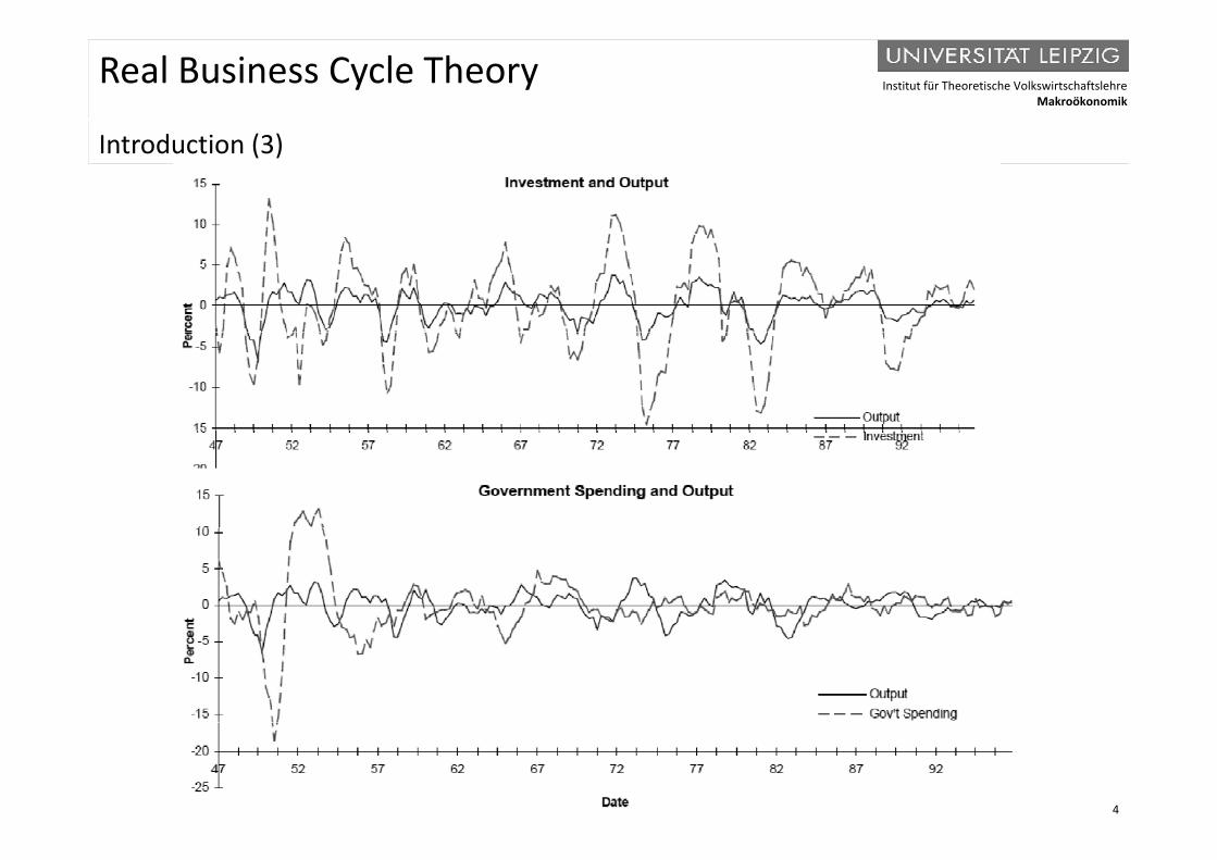
Investment is three times more volatile than output;

Government expenditures are less volatile than output;

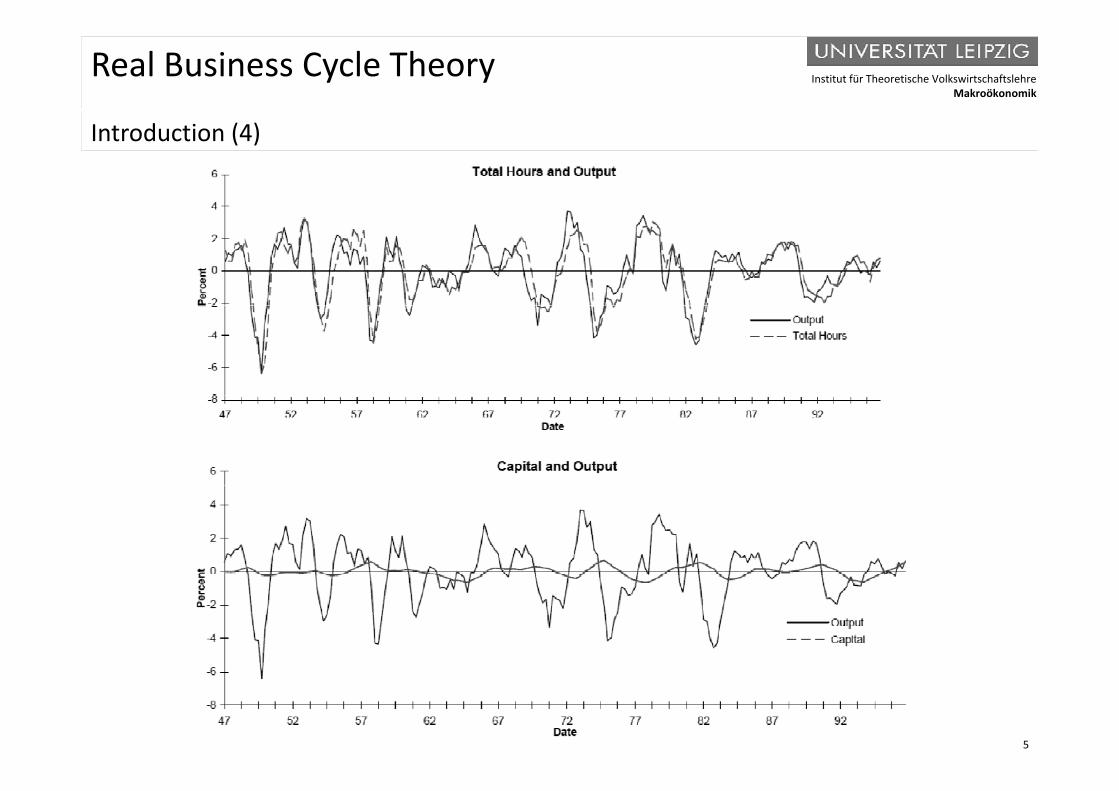
Total hours worked has about the same volatility as output;

Capital is much less volatile than output, but capital utilization in manufacturing is more volatile than output; Capital is much less volatile than output, but capital utilization in manufacturing is more volatile than output;

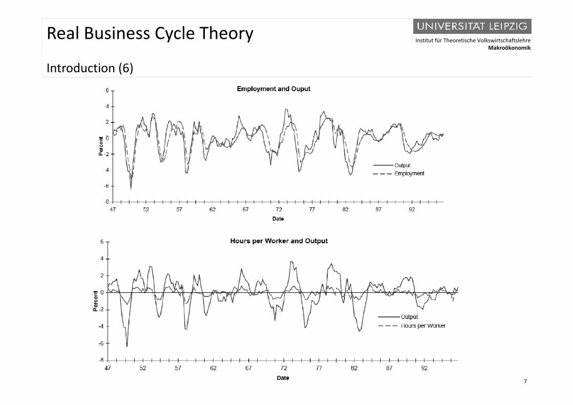
Employment is as volatile as output, while hours per worker are much less volatile than output, so that most of the cyclical variation in total hours worked stems from changes in employment;

Labor productivity (output per man-hour) is less volatile than output; Labor productivity (output per man hour) is less volatile than output;

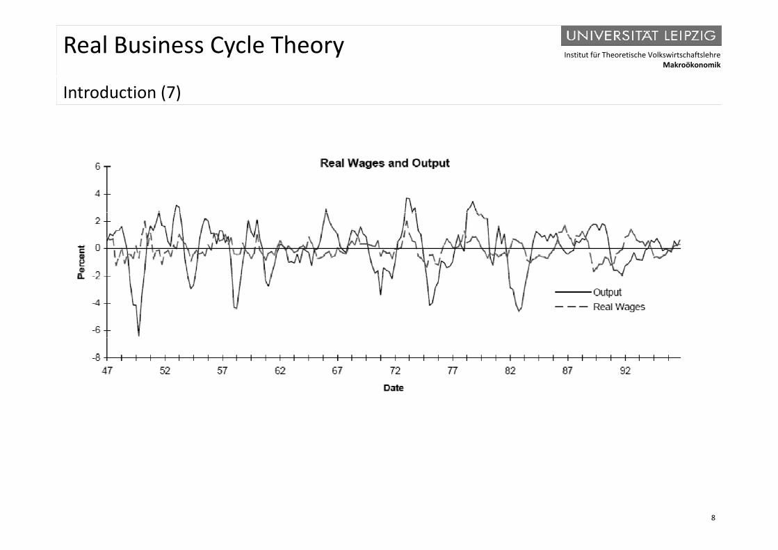
The real wage rate is much less volatile than output.

Comovement. Most macroeconomic series are procyclical, that is, they exhibit a positive contemporaneous correlation with output. The high degree of comovement between total hours worked and aggregate output, displayed above, is particularly striking. Three series are essentially acyclical - wages, government expenditures, and the capital stock - in the sense that their correlation with output is close to zero.

10

Persistence. All macroeconomic aggregates display substantial persistence; the first-order serial correlation for most detrended quarterly variables is on the order of 0.9. This high serial correlation is the reason why there is some predictability to the business cycle.




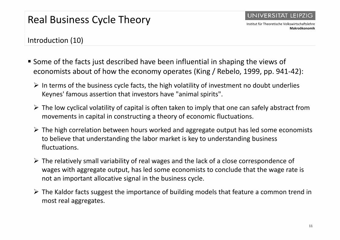
Some of the facts just described have been influential in shaping the views of j p geconomists about of how the economy operates (King / Rebelo, 1999, pp. 941-42):

In terms of the business cycle facts, the high volatility of investment no doubt underlies K ' f ti th t i t h " i l i it "Keynes' famous assertion that investors have "animal spirits".

The low cyclical volatility of capital is often taken to imply that one can safely abstract from movements in capital in constructing a theory of economic fluctuations.

The high correlation between hours worked and aggregate output has led some economists to believe that understanding the labor market is key to understanding business fluctuationsfluctuations.

The relatively small variability of real wages and the lack of a close correspondence of wages with aggregate output, has led some economists to conclude that the wage rate is not an important allocative signal in the business cycle.

The Kaldor facts suggest the importance of building models that feature a common trend in most real aggregates

11

most real aggregates.



A i li ti RBC d l (1)A simplistic RBC model (1)

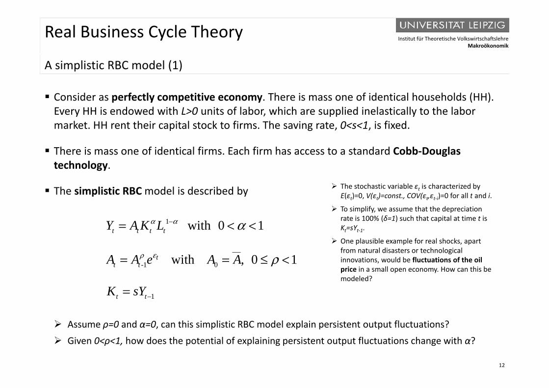
Consider as perfectly competitive economy. There is mass one of identical households (HH). Every HH is endowed with L>0 units of labor, which are supplied inelastically to the labor market. HH rent their capital stock to firms. The saving rate, 0<s<1, is fixed.

There is mass one of identical firms Each firm has access to a standard Cobb Douglas There is mass one of identical firms. Each firm has access to a standard Cobb-Douglas technology.

The simplistic RBC model is described by The stochastic variable εt is characterized by E( ) 0 V( ) t COV( ) 0 f ll t d iThe simplistic RBC model is described by

1 with 0 1t t t tY A K Lα α α−= < <

E(εt)=0, V(εt)=const., COV(εt,εt-i)=0 for all t and i.

To simplify, we assume that the depreciation rate is 100% (δ=1) such that capital at time t is Kt=sYt-1.

1 0- with 0 1, tt tA A e A Aερ ρ= = ≤ <

One plausible example for real shocks, apart from natural disasters or technological innovations, would be fluctuations of the oil price in a small open economy. How can this be modeled?

Assume ρ=0 and α=0 can this simplistic RBC model explain persistent output fluctuations?

1t tK sY −=

12

Assume ρ 0 and α 0, can this simplistic RBC model explain persistent output fluctuations? Given 0<ρ<1, how does the potential of explaining persistent output fluctuations change with α?




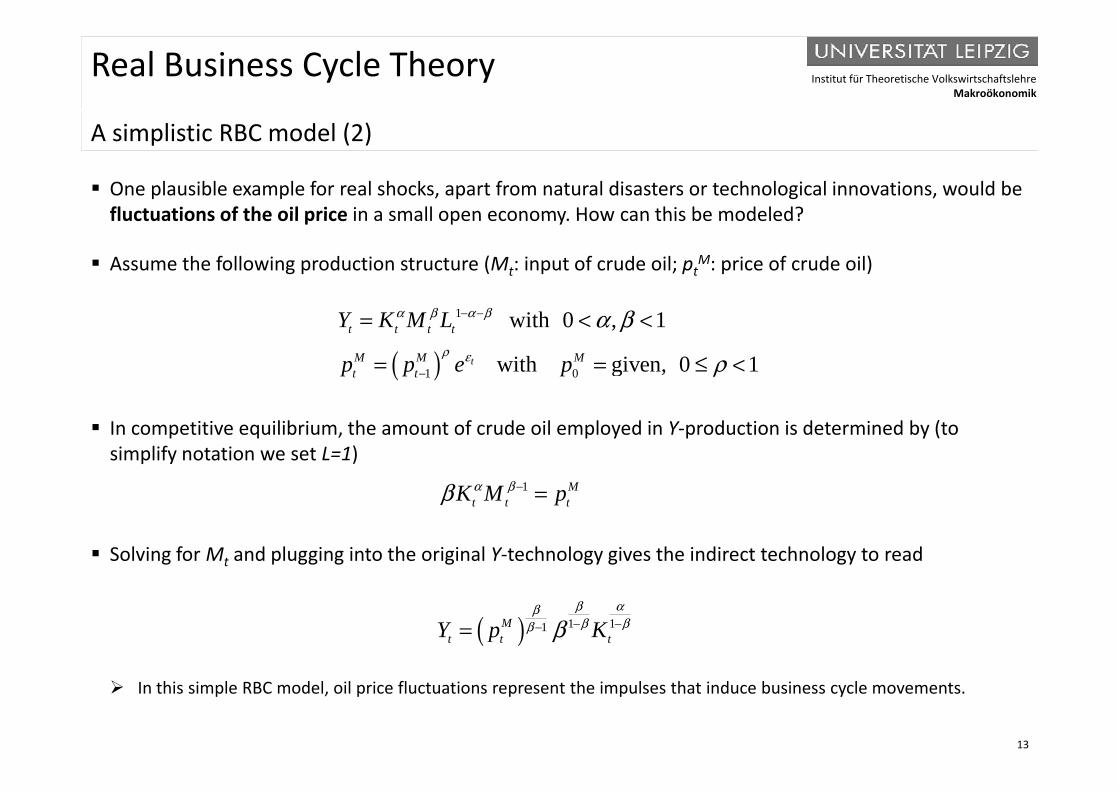
One plausible example for real shocks, apart from natural disasters or technological innovations, would be fluctuations of the oil price in a small open economy How can this be modeled?fluctuations of the oil price in a small open economy. How can this be modeled?

Assume the following production structure (Mt: input of crude oil; ptM: price of crude oil)

( )

1

1 0

with 0 , 1

given 0 1with ,t

t t t t

M M Mt t

Y K M L

p p e p

α β α β

ρ ε

α β

ρ

− −

−

= < <

= = ≤ <

In competitive equilibrium, the amount of crude oil employed in Y-production is determined by (to simplify notation we set L=1)

1 Mα ββ

Solving for Mt and plugging into the original Y-technology gives the indirect technology to read

1 Mt t tK M pα ββ − =

( ) 1 11Mt t tY p K

β αββ ββ β − −−=

13

In this simple RBC model, oil price fluctuations represent the impulses that induce business cycle movements.




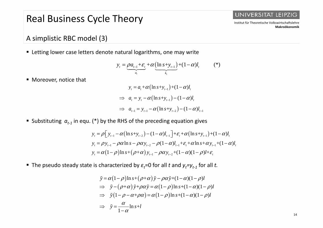
Letting lower case letters denote natural logarithms, one may write

( )

Moreover, notice that

( )1 1+ + ln + (*)+(1 )tt

t t t t t

a k

a y ly sρ ε αα− −= −

( )1+ ln + +(1 )a yy s lαα= −( )( )

( )

1

1

1 1 2 1

+ ln + +(1 )

ln + (1 )

ln + (1 )

t t t t

t t t t

t t t t

a yy s

y s

y s

l

a y l

a y l

α

α

α

α

α

α

−

−

− − − −

− − = −

− = −−

Substituting at-1 in equ. (*) by the RHS of the preceding equation gives

( ) ( )1 2 1 1ln + (1 ) + + ln + +(1 )t t t t t t ty l y ly y s sα αρ α ε α− − − −− −= − −

The pseudo steady state is characterized by ε =0 for all t and y =y for all t

( ) ( )1 2 1 1

1 2

ln (1 ) + + ln + +(1 )

1 ln + + +(1 )(1 ) +t t t t t t t

t t t t

y l y ly y s s

y s y y l

αρ ρ ρ ρ α ε αρ ρ ρ α

α α αα ρα εα

− − − −

− −

− − −

−

= − −

= − −−

The pseudo steady state is characterized by εt=0 for all t and yt=yt-1 for all t.

( ) ( )( ) ( )

1 ln + + +(1 )(1 )+ + 1 ln +(1 )(1 )

y s y yy y

ly s l

ρ ρ ρ α ρρ ρ ρ α ρ

α α αα α α

−= − − = − −

−− −

14

( ) ( )1 + 1 ln +(1 )(1 )

ln +1

y s

y

l

s l

ρ ρα α ρ ρ

α

α αα

= − −− −

=−

−



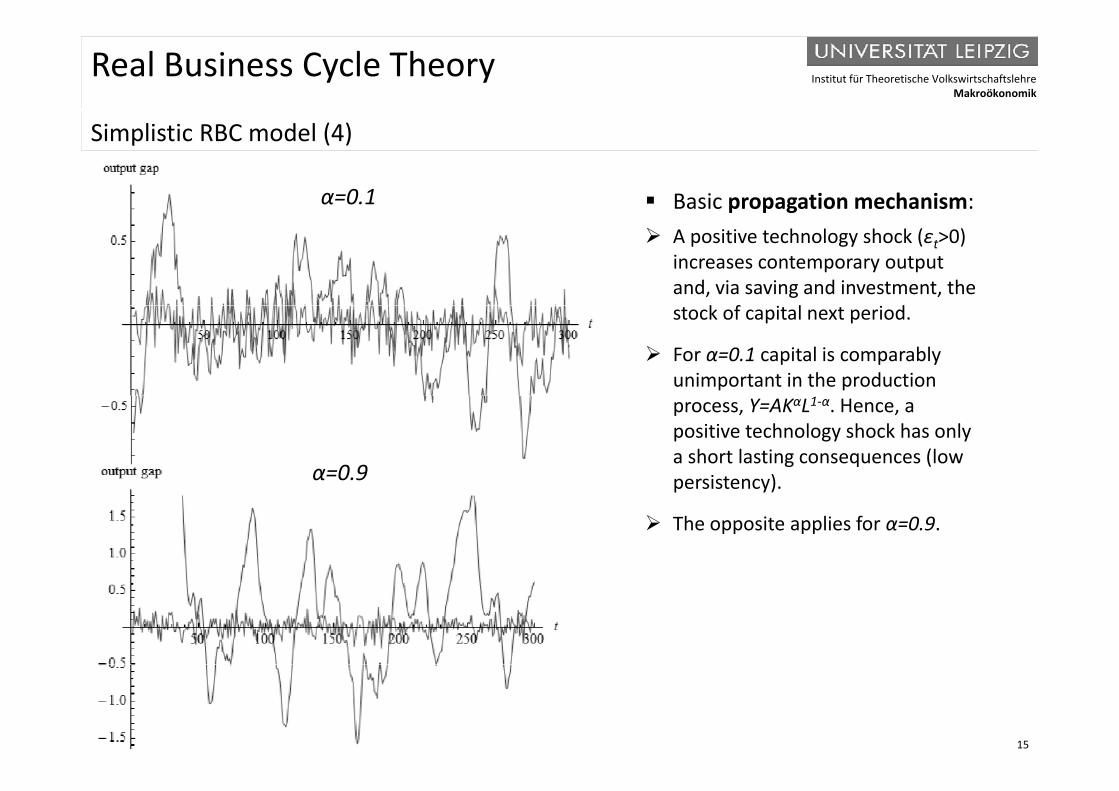
Si li ti RBC d l (4)Simplistic RBC model (4)

Basic propagation mechanism:α=0.1

A positive technology shock (εt>0) increases contemporary output and, via saving and investment, the

k f i l i dstock of capital next period.

For α=0.1 capital is comparably unimportant in the production process, Y=AKαL1-α. Hence, a positive technology shock has only a short lasting consequences (low persistency)α=0.9 persistency).

The opposite applies for α=0.9.

15



St h ti th d l d l tStochastic growth model: model setup

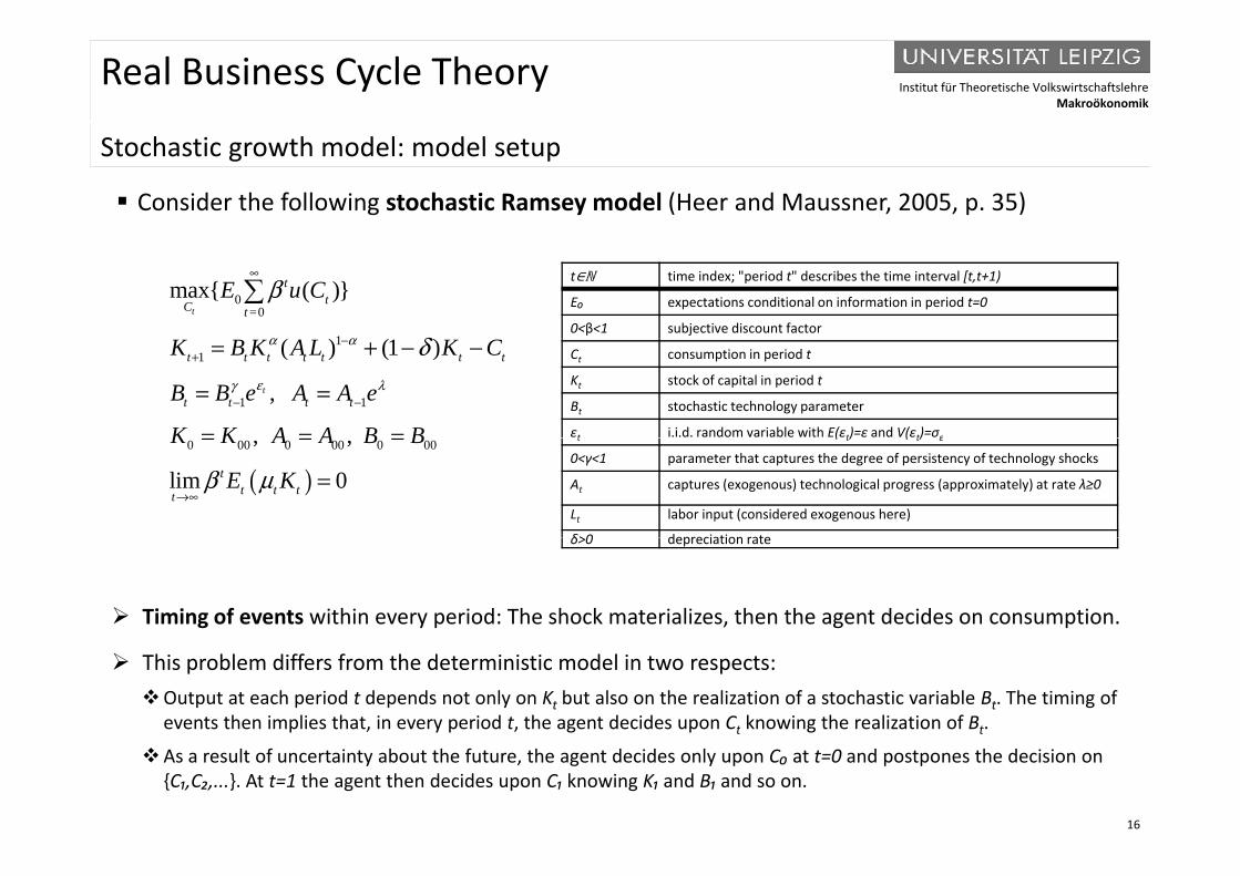
Consider the following stochastic Ramsey model (Heer and Maussner, 2005, p. 35)

00

1

=max{ ( )}

( ) ( )

t

ttC t

E u C

α α

β

δ

∞

t∈ℕ time index; "period t" describes the time interval [t,t+1)

E₀ expectations conditional on information in period t=0

0<β<1 subjective discount factor1

1

1 1

( ) (1 )

,t

t t t t t t t

t t t t

K B K A L K C

B B e A A e

K K A A B B

α α

εγ λ

δ−+

− −

= + − −

= =

= = =

Ct consumption in period t

Kt stock of capital in period t

Bt stochastic technology parameter

εt i.i.d. random variable with E(εt)=ε and V(εt)=σε

( )0 00 0 00 0 00,

li

,

m 0tt t tt

K K A A B B

E Kβ μ→∞

= = =

=

t ( t) ( t) ε

0<γ<1 parameter that captures the degree of persistency of technology shocks

At captures (exogenous) technological progress (approximately) at rate λ≥0

Lt labor input (considered exogenous here)

δ>0 depreciation rate

Timing of events within every period: The shock materializes, then the agent decides on consumption.

δ>0 depreciation rate

This problem differs from the deterministic model in two respects:Output at each period t depends not only on Kt but also on the realization of a stochastic variable Bt. The timing of

events then implies that, in every period t, the agent decides upon Ct knowing the realization of Bt.

16

As a result of uncertainty about the future, the agent decides only upon C₀ at t=0 and postpones the decision on {C₁,C₂,...}. At t=1 the agent then decides upon C₁ knowing K₁ and B₁ and so on.



St h ti th d l d i bl (1)Stochastic growth model: dynamic problem (1)

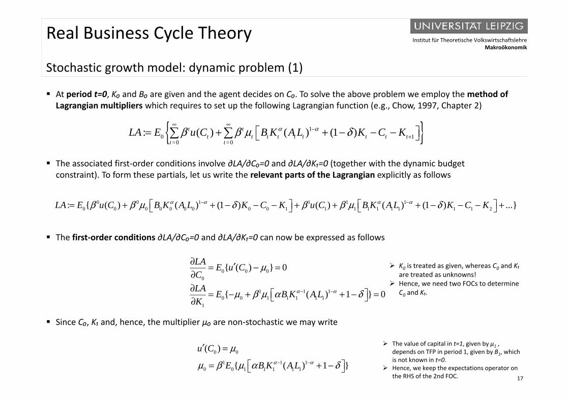
At period t=0, K₀ and B₀ are given and the agent decides on C₀. To solve the above problem we employ the method of Lagrangian multipliers which requires to set up the following Lagrangian function (e.g., Chow, 1997, Chapter 2)

{ }1

0 0= =0 1: ( ) ( ) (1 )t t

t t t t t t t t tt t

E u C B K A L K CLA Kα αβ β μ δ∞ ∞

−+ = + + − − −

g g p q p g g g ( g p )

0 0 1 1 1 1β β δ β β δ

The associated first-order conditions involve ∂LA/∂C₀=0 and ∂LA/∂K₁=0 (together with the dynamic budget constraint). To form these partials, let us write the relevant parts of the Lagrangian explicitly as follows

The first-order conditions ∂LA/∂C₀=0 and ∂LA/∂K₁=0 can now be expressed as follows

0 0 1 1 1 10 0 0 0 0 0 0 0 0 1 1 1 1 1 1 1 1 1 2: { ( ) ( ) (1 ) ( ) ( ) (1 ) ...}E u C B K A L K C K u C B K A L KL KA Cα α α αβ β μ δ β β μ δ− − = + + − − − + + + − − − +

0 0 00

1 1 1

{ ( ) } 0

{ ( ) 1 } 0

E u CCLA

LA E B K A Lα α

μ

β δ− −

∂ ′= − =∂∂ + +

K0 is treated as given, whereas C0 and K₁are treated as unknowns!

Hence, we need two FOCs to determine C and K

Since C₀, K₁ and, hence, the multiplier μ₀ are non-stochastic we may write

1 1 10 0 1 1 1 1 1

1

{ ( ) 1 } 0E B K A LK

α αμ β μ α δ = − + + − = ∂C0 and K₁.

17

0 0

1 1 10 0 1 1 1 1 1

( )

{ ( ) 1 }

u C

E B K A Lα α

μ

μ β μ α δ− −

′ =

= + −

The value of capital in t=1, given by μ1 , depends on TFP in period 1, given by B1, which is not known in t=0.

Hence, we keep the expectations operator on the RHS of the 2nd FOC.




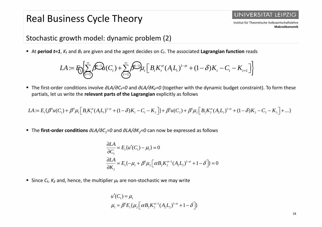
At period t=1, K₁ and B₁ are given and the agent decides on C₁. The associated Lagrangian function reads

{ } The first order conditions involve ∂LA/∂C =0 and ∂LA/∂K =0 (together with the dynamic budget constraint) To form these

{ }1 1 11 1

1 1= =: ( ) ( ) (1 )t t

t t t t t t t t tt t

E u C B K A L K CL KA α αβ β μ δ∞ ∞

− − −+ = + + − − −

The first-order conditions involve ∂LA/∂C₁=0 and ∂LA/∂K₂=0 (together with the dynamic budget constraint). To form these partials, let us write the relevant parts of the Lagrangian explicitly as follows

0 0 1 1 1 11 1 1 1 1 1 1 1 1 2 2 2 2 2 2 2 2 2 3: { ( ) ( ) (1 ) ] ( ) ( ) (1 ) ...}LA E u C B K A L K C K u C B K A L K C Kα α α αβ β μ δ β β μ δ− − = + + − − − + + + − − − +

The first-order conditions ∂LA/∂C1=0 and ∂LA/∂K2=0 can now be expressed as follows

1 1 11

1 1 11 1 2 2 2 2 2

{ ( ) } 0

{ ( ) 1 } 0

E u CCLA

LA E B K A Lα α

μ

μ β μ α δ− −

∂ ′= − =∂∂ = − + + − = ∂

Since C₁, K₂ and, hence, the multiplier μ₁ are non-stochastic we may write

1 1 2 2 2 2 22

{ ( ) }K

μ β μ ∂

18

1 1

1 1 11 1 2 2 2 2 2

( )

{ ( ) 1 }

u C

E B K A Lα α

μμ β μ α δ− −

′ =

= + −




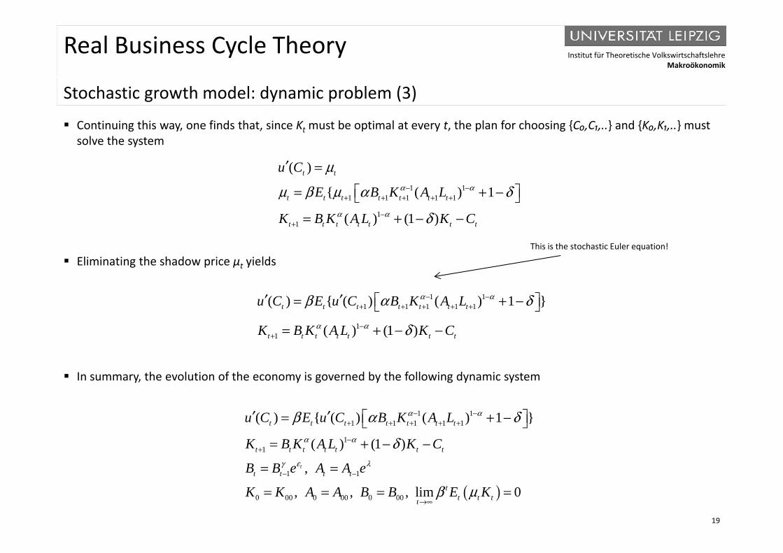
Continuing this way, one finds that, since Kt must be optimal at every t, the plan for choosing {C₀,C₁,..} and {K₀,K₁,..} must solve the system

1 11 1 1 1 1

1

( )

{ ( ) 1

( ) (1 )

t t

t t t t t t t

u C

E B K A L

K B K A L K C

α α

α α

μ

μ β μ α δ

δ

− −+ + + + +

′ =

= + −

Eliminating the shadow price μt yields

11 ( ) (1 )t t t t t t tK B K A L K Cα α δ−

+ = + − −

This is the stochastic Euler equation!

1 11 1 1 1 1

11

( ) { ( ) ( ) 1 }

( ) (1 )

t t t t t t t

t t t t t t t

u C E u C B K A L

K B K A L K C

α α

α α

β α δ

δ

− −+ + + + +

−+

′ ′ = + −

= + − −

In summary, the evolution of the economy is governed by the following dynamic system

1 11 1 1 1 1

11

( ) { ( ) ( ) 1 }

( ) (1 )t t t t t t t

t t t t t t t

u C E u C B K A L

K B K A L K C

B B A A

α α

α α

εγ λ

β α δ

δ

− −+ + + + +

−+

′ ′ = + −

= + − −

19

( )1 1

0 00 0 00 0 00

,

, , , lim 0

tt t t t

tt t tt

B B e A A e

K K A A B B E K

εγ λ

β μ− −

→∞

= =

= = = =



St h ti th d l l k FOCStochastic growth model: general remark on FOC

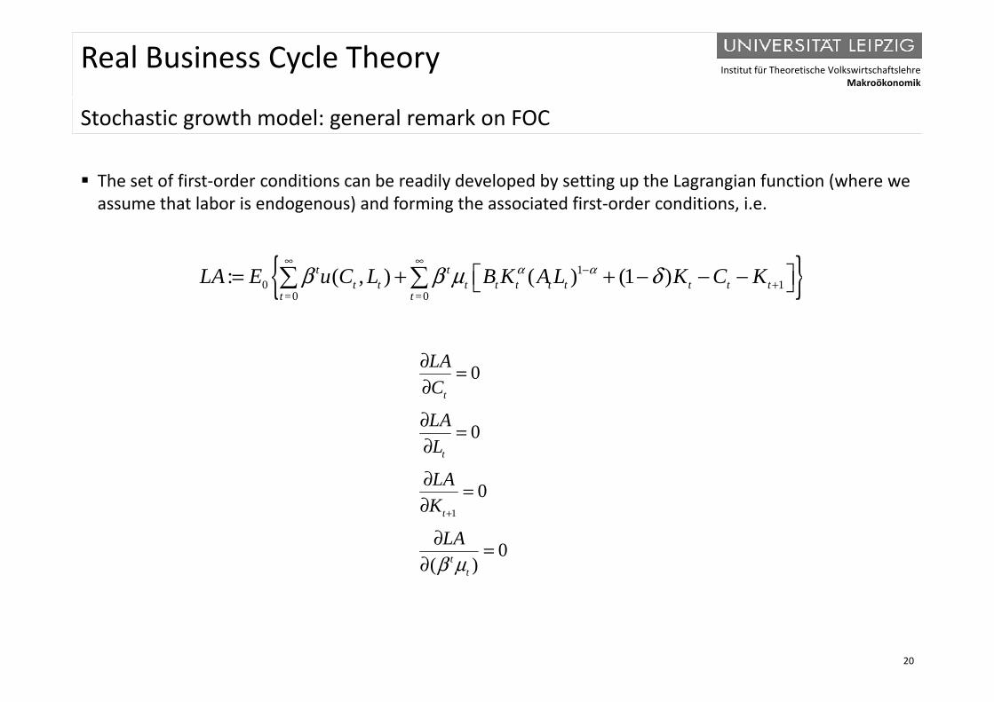
The set of first-order conditions can be readily developed by setting up the Lagrangian function (where we assume that labor is endogenous) and forming the associated first-order conditions, i.e.

{ }1( ) ( ) (1 )t tE C L B K A KA C KL Lα αβ β δ∞ ∞

− { }10 1

0 0= =: ( ) ( ) (1 ),t t

t t t t t t t t t tt t

E u C L B K A KA C KL Lα αβ β μ δ + = + + − − −

0

0

t

LA

LA

C∂ =∂

∂ =

1

0

0

t

L

L

AK

=∂

∂ =∂ 1

0( )

t

tt

K

LAβ μ

+∂

∂ =∂

20



St h ti th d l d t i i ti d i t d t d t tStochastic growth model: deterministic dynamic system and steady state

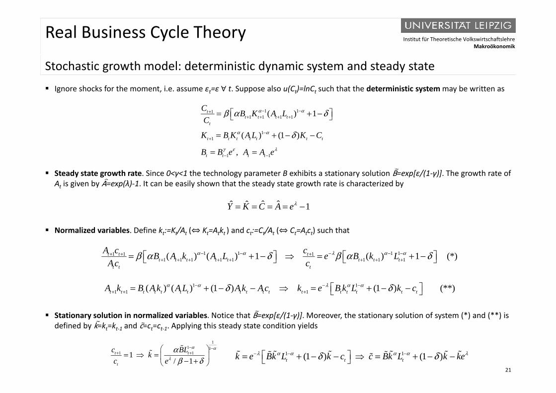
Ignore shocks for the moment, i.e. assume εt=ε ∀ t. Suppose also u(Ct)=lnCt such that the deterministic system may be written as

C 1 111 1 1 1

11

( ) 1

( ) (1 )

tt t t t

t

t t t t t t t

C B K A LC

K B K A L K C

B B e A A e

α α

α α

γ ε λ

β α δ

δ

− −++ + + +

−+

= + −

= + − −

= =

Steady state growth rate. Since 0<γ<1 the technology parameter B exhibits a stationary solution B=exp[ε/(1-γ)]. The growth rate of At is given by A=exp(λ)-1. It can be easily shown that the steady state growth rate is characterized by

1 1,t t t tB B e A A e− −= =

Normalized variables. Define kt:=Kt/At (⇔ Kt=Atkt ) and ct:=Ct/At (⇔ Ct=Atct) such that

ˆ ˆˆ ˆ 1Y K C A eλ= = = = −

1 1 1 11 1 11 1 1 1 1 1 1 1( ) (( ) 1 *)( ) 1t t t

t t t t t t t tt t t

A c cB A k A L e B k LAc c

α α λ α αβ α δ β α δ− − − − −+ + ++ + + + + + + + = + − = + −

1 1( ) ( ) (1 ) (1 ) (**)A k B Ak A L Ak A k B k L kα α λ α αδ δ− − −

Stationary solution in normalized variables. Notice that B=exp[ε/(1-γ)]. Moreover, the stationary solution of system (*) and (**) is defined by k=kt=kt-1 and c=ct=ct-1. Applying this steady state condition yields

1 11 1 1( ) ( ) (1 ) (1 ) (**)t t t t t t t t t t t t t t t t tA k B Ak A L Ak Ac k e B k L k cα α λ α αδ δ+ + + = + − − = + − −

21

t t 1 t t 1

11 1

1 11/ 1

t t

t

c BLkc e

α α

λ

αβ δ

− −+ +

= = − +

1 1(1 ) (1 )t t tk e Bk L k c c Bk L k keλ α α α α λδ δ− − − = + − − = + − −



St h ti th d l i l f tiStochastic growth model: impulse-response functions

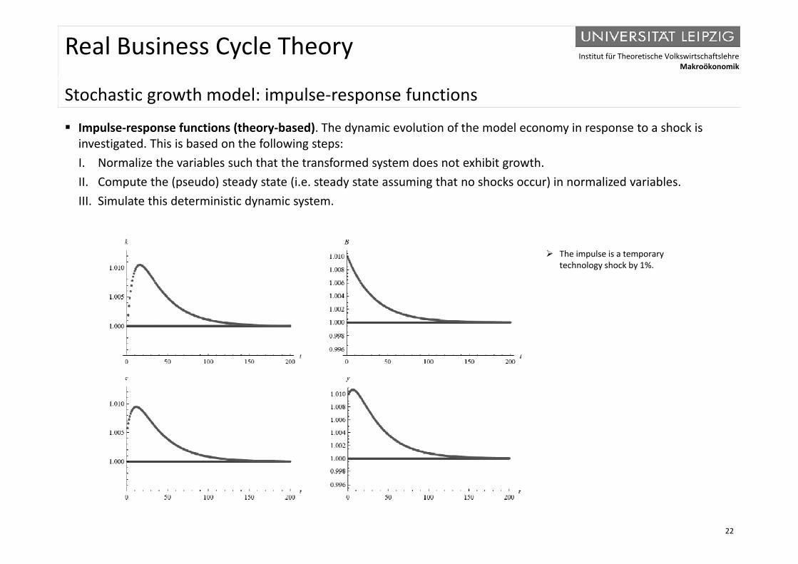
Impulse-response functions (theory-based). The dynamic evolution of the model economy in response to a shock is investigated. This is based on the following steps: I. Normalize the variables such that the transformed system does not exhibit growth.II. Compute the (pseudo) steady state (i.e. steady state assuming that no shocks occur) in normalized variables.III. Simulate this deterministic dynamic system.

The impulse is a temporary technology shock by 1%.

22



B i RBC d l d l tBasic RBC model: model setup

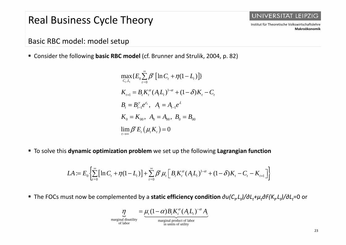
Consider the following basic RBC model (cf. Brunner and Strulik, 2004, p. 82)

[ ]00

11

, =max{ ln (1 ) }

( ) (1 )

t t

tt tC t

t t t t t t t

LE C L

K B K A L K Cα α

β η

δ

∞

−+

+ −

= + − −

1

1 1

0 00 0 00 0 00

( ) ( )

, ,

,t

t t t t t t t

t t t tB B e A A e

K K A A B B

εγ λ

+

− −= =

= = =

To solve this dynamic optimization problem we set up the following Lagrangian function

( )lim 0tt tt tE Kβ μ

→∞=

To solve this dynamic optimization problem we set up the following Lagrangian function

[ ]{ }1

0 00 1: ln (1 ) ( ) (1 )t

t t t t t t t t t tE C L B A LL K C KA Kα αη β μ δ∞ ∞

−+ = + − + + − − −

The FOCs must now be complemented by a static efficiency condition ∂u(Ct,Lt)/∂Lt+μt∂F(Kt,Lt)/∂Lt=0 or

{ }0 0==t t

23

marginal disutilit marginal product of laboy

of laborr

in untits of utility

(1 ) ( )t t t t t tB K A L Aα αη μ α −= −



B i RBC d l d i tBasic RBC model: dynamic system

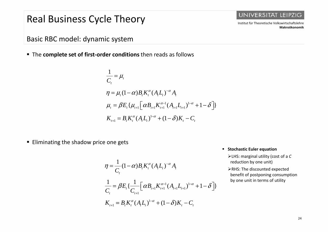
The complete set of first-order conditions then reads as follows

1t

tCμ=

1 11 1 1 1 1

1

(1 ) ( )

{ ( ) 1 }

( ) (1 )

t t t t t t

t t t t t t t

B K A L A

E B K A L

K B K A L K C

α α

α α

α α

η μ α

μ β μ α δ

δ

−

− −+ + + + +

= −

= + −

Eliminating the shadow price one gets


+ = + − −

Eliminating the shadow price one gets

1 (1 ) ( )t t t t tB K A L AC

α αη α −= −

Stochastic Euler equationLHS: marginal utility (cost of a C

reduction by one unit)RHS: The discounted expected

1 11 1 1 1

1

( ) ( )

1 1{ ( ) 1 }

t t t t tt

t t t t tt t

C

E B K A LC C

α α

η

β α δ− −+ + + +

+

= + −

RHS: The discounted expected benefit of postponing consumption by one unit in terms of utility

24


+ = + − −



B i RBC d l d t i i ti d i t d t d t tBasic RBC model: deterministic dynamic system and steady state

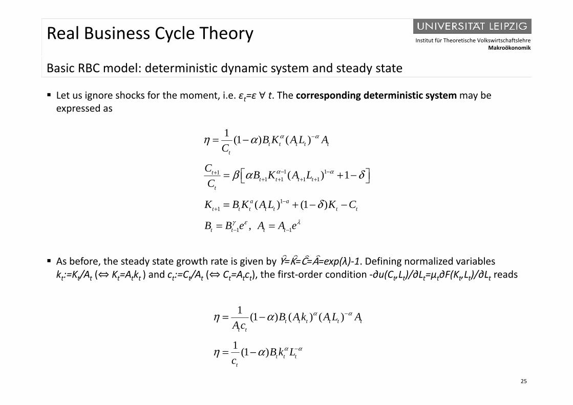
Let us ignore shocks for the moment, i.e. εt=ε ∀ t. The corresponding deterministic system may be expressed asexpressed as

1 (1 ) ( )t t t t tt

B K A L AC

α αη α −= −

1 111 1 1 1

1

( ) 1

( ) (1 )

tt t t t

t

a a

C B K A LC

K B K A L K C

α αβ α δ

δ

− −++ + + +

−

= + −

+11

1 1

( ) (1 )

,

a at t t t t t t

t t t t

K B K A L K C

B B e A A eγ ε λ

δ+

− −

= + − −

= =

As before, the steady state growth rate is given by Y=K=C=A=exp(λ)-1. Defining normalized variables kt:=Kt/At (⇔ Kt=Atkt ) and ct:=Ct/At (⇔ Ct=Atct), the first-order condition -∂u(Ct,Lt)/∂Lt=μt∂F(Kt,Lt)/∂Lt reads

1 (1 ) ( ) ( )t t t t t tt t

B A k A L AAc

α αη α −= −

25

1 (1 ) t t tt

B k Lc

α αη α −= −



B i RBC d l d i t d t d t tBasic RBC model: dynamic system and steady state

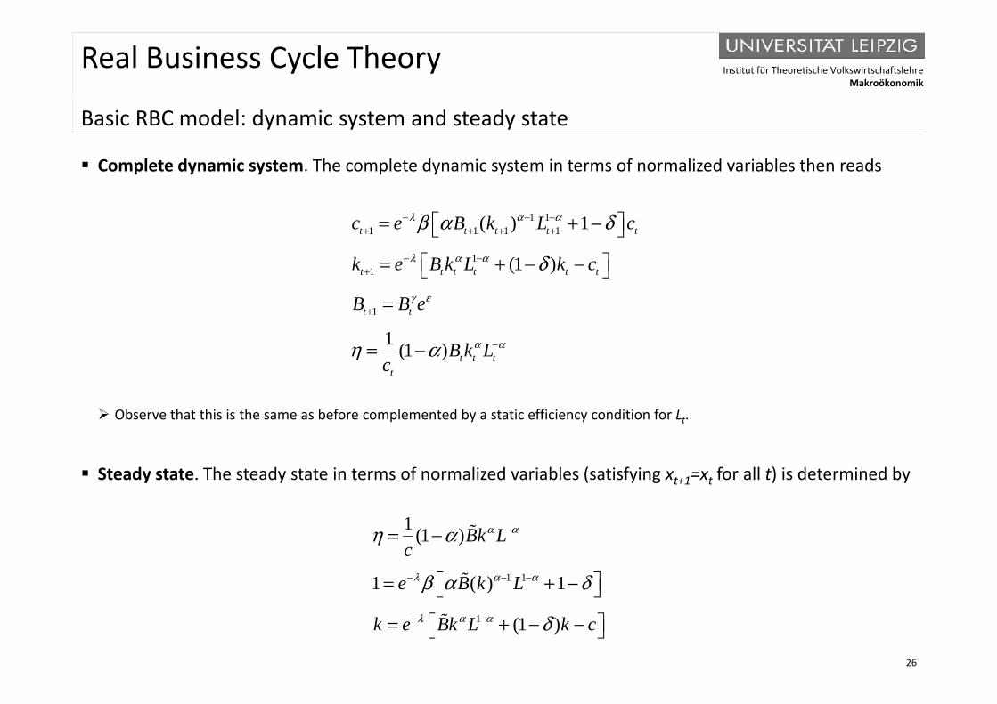
Complete dynamic system. The complete dynamic system in terms of normalized variables then reads

1 11 1 1 1

11

( ) 1

(1 )

t t t t t

t t t t t t

c e B k L c

k e B k L k c

λ α α

λ α α

β α δ

δ

− − −+ + + +

− −+

= + −

= + − − 1

1

( )

1 (1 )

t t t t t t

t tB B e

B k L

γ ε

α αη α

+

+

−

=

= −

Observe that this is the same as before complemented by a static efficiency condition for Lt.

(1 ) t t tt

B k Lc

η α=

Steady state. The steady state in terms of normalized variables (satisfying xt+1=xt for all t) is determined by

1 1

1 (1 )

1 ( ) 1

Bk Lc

e B k L

α α

λ α α

η α

β α δ

−

− − −

= −

= + −

26

1

( )

(1 )k e Bk L k cλ α α

β

δ− −

= + − −



B i RBC d l i l f ti (1)Basic RBC model: impulse-response functions (1)

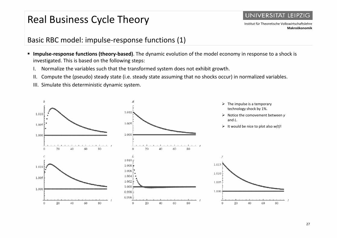
Impulse-response functions (theory-based). The dynamic evolution of the model economy in response to a shock is investigated. This is based on the following steps: I. Normalize the variables such that the transformed system does not exhibit growth.II. Compute the (pseudo) steady state (i.e. steady state assuming that no shocks occur) in normalized variables.III. Simulate this deterministic dynamic system.

The impulse is a temporary technology shock by 1%.

Notice the comovement between yd Land L.

It would be nice to plot also w(t)!

27



B i RBC d l i l f ti (2)Basic RBC model: impulse-response functions (2)

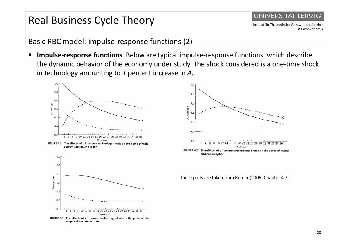
Impulse-response functions. Below are typical impulse-response functions, which describe the dynamic behavior of the economy under study. The shock considered is a one-time shock y y yin technology amounting to 1 percent increase in At.

These plots are taken from Romer (2006; Chapter 4.7).p ( ; p )

28



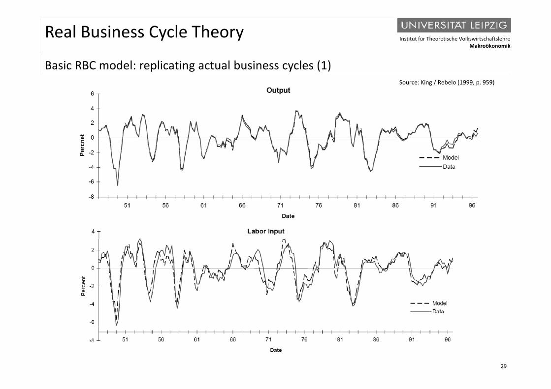
B i RBC d l li ti t l b i l (1)Basic RBC model: replicating actual business cycles (1)Source: King / Rebelo (1999, p. 959)

29



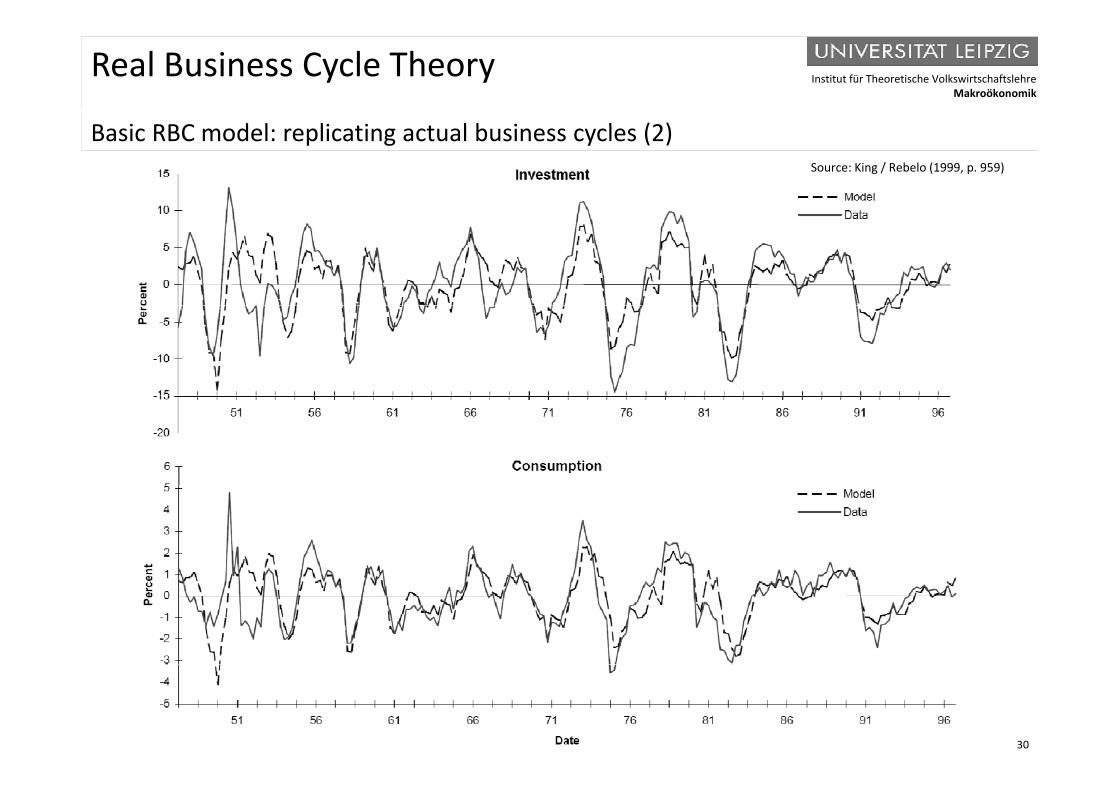
B i RBC d l li ti t l b i l (2)Basic RBC model: replicating actual business cycles (2)Source: King / Rebelo (1999, p. 959)

30



C i f th ti l d i i l tComparison of theoretical and empirical moments

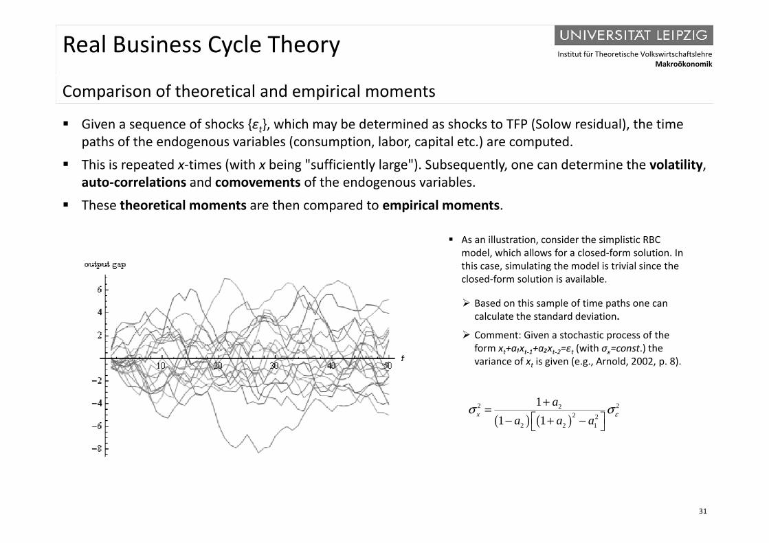
Given a sequence of shocks {εt}, which may be determined as shocks to TFP (Solow residual), the time paths of the endogenous variables (consumption, labor, capital etc.) are computed.p g ( p p ) p

This is repeated x-times (with x being "sufficiently large"). Subsequently, one can determine the volatility, auto-correlations and comovements of the endogenous variables.

These theoretical moments are then compared to empirical moments. p p

As an illustration, consider the simplistic RBC model, which allows for a closed-form solution. In this case, simulating the model is trivial since the closed-form solution is available.

Based on this sample of time paths one can calculate the standard deviation.

Comment Gi en a stochastic process of the Comment: Given a stochastic process of the form xt+a₁xt-1+a₂xt-2=εt (with σε=const.) the variance of xt is given (e.g., Arnold, 2002, p. 8).

( ) ( )2 22

2 22 2 1

11 1x

aa a a εσ σ+=

− + −

31



S d l iSummary and conclusion

The RBC model represents a neoclassical economy where real shocks drive output d land employment movements.

The underlying model economy is perfect and, hence, the movements are optimal t h k P t diff tl b d t t t d l tresponses to shocks. Put differently, observed aggregate output and employment

movements are interpreted to represent time-varying Pareto-optimal equilibria.

Thus contrary to conventional wisdom macroeconomic fluctuations do not reflect Thus, contrary to conventional wisdom, macroeconomic fluctuations do not reflect any market failures, and government interventions to mitigate them can only reduce welfare.

The notion that adverse downward movements in total technology cause recessions is just plain silly. This is the theory according to which the 1930s should be known

h G D i b h G V i (M 1998 384)not as the Great Depression but as the Great Vacation. (Mussa, 1998, p. 384)

The RBC research program has initiated the DSGE methodology. This set of t h i h b li d t i l ithi th t t f th

32

techniques has been applied extensively within the context of other macroeconomic theories, most prominently the New Keynesian Theories.



N t tiNotation

A exogenous technological progress 0<α<1 technology parameterAt exogenous technological progress Bt stochastic technology parameterCt consumption ct:=Ct/At normalized consumption

0<α<1 technology parameter 0<β<1 subjective discount factor0<γ<1 parameter indicating persistency of technology shocksδ≥0 capital depreciation rate t t t

Et expectations in period tKt stock of capitalkt:=Kt/At normalized capital

εt i.i.d. random variable with E(εt)=ε≥0 and V(εt)=σε

η>0 preference parameterλ≥0 rate of technological progress

l lLA Lagrangian functionLt labor input 0<s<1 saving rate u( ) instantaneous utility

μt Lagrangian multiplier

ρ>0 time preference rate σ standard deviation

u(.) instantaneous utilityYt final output at time tỹ pseudo steady state

33

3. real business cycle theory - uni-leipzig.de · institut für theoretische volkswirtschaftslehre...

Documents