2d burgers equations with large reynolds number using pod
TRANSCRIPT

2D Burgers Equations with LargeReynolds Number Using POD/DEIM
and Calibration
Yuepeng Wanga), I.Michael Navonb)∗ , Xinyue Wangc), Yue Chengd)
a,d)School of Mathematics and StatisticsNanjing University of Information Science and Technology (NUIST ), Nanjing, China, 210044
[email protected])Department of Scientific Computing
F lorida State University, Tallahassee, FL 32306, U.S.A∗[email protected]
c)School of Atmospheric ScienceNanjing University of Information Science and Technology (NUIST ), Nanjing, China, 210044
Abstract: Model order reduction (MOR) of the 2D Burgers equation is investigated. The mathematical formulation of POD/DEIM reduced order model (ROM) is derived based on the Galerkin projection and discrete empirical interpolation method (DEIM) from the existing high fidelity implicit finite difference full model. For validation we numerically compared the POD ROM, POD/DEIM and the full model in two cases of Re = 100 and Re = 1000, respectively. We found that the POD/DEIM ROM leads to a speed-up of CPU time by a factor of O(10). The computational stability of POD/DEIM ROM is maintained by means of a careful selection of POD modes and the DEIM interpolation points. The solution of POD/DEIM in the case of Re = 1000 has an accuracy with error O(10−3) versus O(10−4) in the case of Re = 100 when compared to the high fidelity model. For this turbulent flow, a closure model consisting of a Tikhonov regularization is carried out in order to recover the missing information and is developed to account for the small scale dissipation effect of the discarded POD modes. It is shown that the computational results of this calibrated low-order model (LOM) exhibit considerable agreement with the real high-fidelity model, which implies the efficiency of the closure model used.
Keywords: 2D Burgers equation; POD/DEIM reduced order Model; Tikhonov regu-larization; Calibration
1 Introduction
The two-dimensional Burgers’ equation is a fundamental mathematical modelfrom fluid mechanics which has the same convective and diffusion terms as theNavier-Stokes equation, and is widely used in various areas as a simple modelfor understanding of various physical flows and problems, such as modelingof dynamics, the phenomena of turbulence, and flow through a shock wavetraveling in a viscous fluid and traffic flow [1, 2, and 3]. Numerical solutionof Burgers equation is a logical first step towards developing methods for the
1

computation of complex flows. Burgers equation is also a useful tool for ex-amining the robustness of numerical discretization schemes [4]. It has becomecustomary to test new numerical approaches in computational fluid dynamicsby implementing novel numerical approaches to the Burgers equation. So far,many numerical solution approaches to 2D Burgers equations have been devel-oped by scientists and engineers, such as [3,5,6,7]. In addition, its analyticalsolution was also explored [8]using the Cole-Hopf transformation.
However, in the conventional numerical approach the computational costof these calculations becomes higher as the Reynolds number (Re) increas-es, particularly when a smooth wave becomes a single-shock wave. Also thecost increases as we refine the resolution of the spatial discretization mesh.This will become more accentuated when attempting to solve a control or pdeoptimization problem in a wide class of engineering applications by DNS (di-rect numerical simulation) of the full 2D Burgers equations model due to therequirement of quick and repeated numerical simulations[9,10,11,12], which of-ten pose important mathematical and computational challenges in both CPUand memory requirements.
To overcome the difficulty encountered during simulating, controlling, andoptimizing such systems, reduced-order modelling offers a possible remedy asa powerful and feasible approach enabling a representation of the dynamics ofhigh-dimensional systems on a smaller number of degrees of freedom. Devel-oping low-dimensional models for partial differential equations (PDEs) is oneof the active research topics today [13,14].
An effective technique of low-order modelling, Proper Orthogonal Decom-position (POD) is attractive to apply [15,16], and has become one of the mostimportant reduced order model (ROM) methods combined with Galerkin pro-jection, thanks to its ability to rebuild numerical signals, with a high order ofprecision gained with only few POD-modes. Additionally, POD is also knownunder other names such as Karhunen-Love expansions [17,18], principal com-ponent analysis [19], empirical orthogonal functions [20], and the Hotellingtransform [21]. It is one of the most prevalent model reduction methods fornonlinear problems [13]. Data analysis using POD is conducted in order toextract basis functions from experimental data or detailed simulations of high-dimensional systems for subsequent use in Galerkin projections that yield low-dimensional dynamical models. Nevertheless, beside its efficiency, the PODGalerkin approach still exhibits some disadvantages.
First, for models with nonlinear terms, the nonlinear reduced terms stillhave to be evaluated on the original state space making the simulation of thereduced order system computationally expensive. Presently an interpolationtechnique known as discrete empirical interpolation method (DEIM) [22,23,24]is the best candidate method that avoids this problem by using an interpola-tion algorithm [25,26,27]. DEIM approach employs a small selected a set ofspatial grid points to avoid evaluation of the expensive inner products at ev-
2
ery time step that are required to evaluate the nonlinear term and focuses onapproximating each nonlinear function so that a certain coefficient matrix canbe precomputed and, as a result, the complexity in evaluating the nonlinearterm is proportional to only a small number of selected spatial indices, thus aconsiderable reduction in complexity is achieved.
Second, for the conventional POD-ROM, few modes are sufficient to perfor-m a feasible computation and give a good representation of the kinetic energyof the flow, however, the low-order ODE systems obtained are unstable flowwith high Reynolds number due to the discarded POD modes. This is dueto discarded small singular values through which energy dissipation occurs inoverall dynamical system [28,29]. This can bring about a lack of effectivenessand stability of the POD-Galerkin method [30,31]. Thus robustness is stillan issue in turbulent POD-Galerkin ROM. To fix and improve the accura-cy and stability of such POD-based reduced-order models, various calibrationmethods were proposed, such as H1 Sobolev norm [14,32,and 33], eddy viscosi-ties [34], least square or adjoint method [30,35,36,37,38]. Calibration of LOMcan enhance its performance at low computational cost, but still remains achallenging task.
When the one-dimensional Burgers equation is considered, the correspond-ing POD/DEIM reduced order model has been developed, and the controlproblem involved was also discussed. It has been shown in [39,40,41,42] thatgood results are achieved. Yet to the best of our knowledge, there are veryfew results reporting the POD/DEIM reduced order modeling issues for 2DBurgers equation, particularly in the case where the Reynolds number be-comes large, and the question remains if the use of a proper number of DEIMpoints is really beneficial for POD/DEIM CPU cost. This paper fills the gapbetween very simple models and very complicated systems such as those re-ported in [43]. The present work can be viewed as a new step towards the goalof modeling and control of more complicated PDE systems.
The main focus of the paper is the size of the reduced order system and thequality of approximation compared to the full-order system, as well as compu-tational efficiency gained by using POD/DEIM in nonlinear model reductionapplications to 2D Burgers equation. Even though these are some fundamen-tal questions related to POD, we believe that they have not been addressed inliterature related to 2D Burgers equations with large Reynolds number (Re).
The main contributions of the research presented in this paper are , first,development of the mathematical formulation of POD/DEIM ROM basedon existing fully implicit finite difference time discretization scheme; second,derivation of a calibrated low order ODEs system from the precomputed PODcoefficients using the Tikhonov regularization method as closure model in thecase where we deal with a large Re [44] (due to the rather demanding mem-ory requirements, we had to restrict the turbulent case only to Re numberequal to 1000). It is expected that a reduced-order ODEs model of the two-
3

dimensional Burgers equation can yield a decrease in both the memory storagerequirements and the CPU time.
The rest of this paper is organized as follows. Section II provides theconstruction process of the POD/DEIM reduced order model of 2D Burger-s equation, including: description of two-dimensional Burgers equation andfully implicit finite difference scheme in section 2.1, and the correspondingNewton iteration method in section 2.2, the POD ROM of 2D Burgers equa-tion and Galerkin projection are presented in section 2.3, as well as discreteempirical interpolation method (DEIM) dealing with the nonlinear functionsarising from the nonlinear advection terms in the 2-D Burgers model in sec-tion 2.4, while in section 2.5, numerical experiments are performed to verifyand validate the POD/DEIM ROM in the case of Re = 100 and Re = 1000,respectively. Special care needs to be taken to find the reduced basis and tochoose DEIM interpolation points. In Section 3, a calibrated LOM based onTikhonov regularization method serving as a closure model is developed forturbulent flow (Re = 1000). Concluding remarks are provided at the end ofthe paper, and an Appendix providing a simple introduction to the discretePicard condition is added for better presentation of the regularization closuremodel.
2 POD/DEIM reduced order model of
2D Burgers equation
Considering the construction of POD or POD/DEIM ROM, some important details about the f ully implicit finite difference scheme and its Newton iteration solution method are stressed here, and presented in sections 2.1 and 2.2, respectively.
2.1 Full-order Model of 2D Burgers equation
We consider a two-dimensional nonlinear viscous Burgers equations like this(called Full Model):
∂u
∂t+ u
∂u
∂x+ v
∂u
∂y=
1
Re(∂2u
∂x2+∂2u
∂y2), (2.1.1a)
∂v
∂t+ u
∂v
∂x+ v
∂v
∂y=
1
Re(∂2v
∂x2+∂2v
∂y2), (2.1.1b)
(x, y) ∈ Ω = (a, b)× (c, d), t ∈ (0, T )
subject to the boundary conditions
u(a, y, t) = gu1(y, t); u(b, y, t) = gu2(y, t);
4

u(x, c, t) = gu3(x, t); u(x, d, t) = gu4(x, t); (2.1.2a)
v(a, y, t) = gv1(y, t); v(b, y, t) = gv2(y, t);
v(x, c, t) = gv3(x, t); v(x, d, t) = gv4(x, t); (2.1.2b)
and the initial conditions
u(x, y, t)|t=0 = φ(x, y), (2.1.2c)
v(x, y, t)|t=0 = ψ(x, y), (x, y) ∈ Ω (2.1.2d)
where Re is the Reynolds number, and the u(x, y, t) and v(x, y, t)represent thevelocity components, respectively. When 2D spatial computational domain Ωis divided uniformly into nx − 1 and ny − 1 subintervals in x and y direction,respectively. It is assumed that the discrete functions are defined on an nx×ny
-grids in space domain Ω = [a, b] × [c, d] . The following notation will beused: xj = jdx, yi = idy, uij = u(xi, yj, t), vij = v(xi, yj, t) . Here dx =b−anx−1
, dy = d−cny−1
. Then the centered-difference scheme corresponding to the
first- or second-order derivatives in space will eventually result in the followingform of 2D Burgers equation[3]:
dui,jdt
+ui+1,j − ui−1,j
2dxui,j +
ui,j+1 − ui,j−1
2dyvi,j =
1
Redx2(ui+1,j − 2ui,j + ui−1,j) +
1
Redy2(ui,j+1 − 2ui,j + ui,j−1) (2.1.3a)
dvi,jdt
+vi+1,j − vi−1,j
2dxui,j +
ui,j+1 − vi,j−1
2dyvi,j =
1
Redx2(vi+1,j − 2vi,j + vi−1,j) +
1
Redy2(vi,j+1 − 2vi,j + vi,j−1) (2.1.3b)
which can be cast in matrix form as follows:
dU
dt+ f1(U, V )− 1
2dxBulU − 1
2dyBubV =
1
Redx2(D1U + b1u) +
1
Redy2(D2U + b2u) (2.1.4a)
dV
dt+ f2(U, V )− 1
2dxBvlU − 1
2dyBvbV =
1
Redx2(D1V + b1v) +
1
Redy2(D2V + b2v) (2.1.4b)
where
U = (u1,1, u2,1, · · · , un,1, u1,2, · · · , un,2, · · · , u1,n, · · · , un,n)T
5

V = (v1,1, v2,1, · · · , vn,1, v1,2, · · · , vn,2, · · · , v1,n, · · · , vn,n)T
hereafter, the superscript ‘T ’ stands for transpose. Let nxy = (nx−2)×(ny−2), two maps f1, f2 : R
nxy ×Rnxy → Rnxy are then defined as follows:
f1(U, V ) =1
2dxMU. ∗ U +
1
2dyNU. ∗ V, (2.1.5a)
f2(U, V ) =1
2dxMV. ∗ U +
1
2dyNV. ∗ V, (2.1.5b)
and M =
M1
. . .
M1
(ny−2)×(ny−2)
, M1 =
0 1
−1. . . 1−1 0
(nx−2)×(nx−2)
with ‘.∗’ denoting componentwise multiplication as used in Matlab; theBul,Bub,b1uand b2uare related to the boundary conditions, which are denoted by
Bul = diag(kron(u(1, 2 : ny − 1), [1, 0, 0, · · · , 0]1×(nx−2))),
Bub = diag(kron([1, 0, 0, · · · , 0]1×(ny−2), u(2 : nx − 1, 1)),
b1u = (u1,2, 0, · · · , 0, u5,2, u1,3, 0, · · · , u5,4)T ,
b2u = [u(2 : nx − 1, 1)T , 0, · · · , 0, u(2 : nx − 1, 5)T ]T ,
D1 =
D11
. . .
D11
(ny−2)×(ny−2)
, D2 =
−2E(nx−2)×(nx−2) E
E. . . EE −2E
(ny−2)×(ny−2)
D11 =
−2 1
1. . . 11
(nx−2)×(nx−2)
, N =
E
−E . . .
−E E
where E is (ny − 2)-by-(ny − 2) the identity matrix, and ‘kron’ is a Matlabfunction which means that K = kron(A,B) returns the Kronecker tensorproduct of A and B. Note that Bvl,Bvb,b1v and b2v are not mentioned here dueto their same expression with Bul,Bub,b1u and b2u.
2.2 Newton method of Full-order Model
Equations (2.1.4a,b) is just a semi-discretized system (ODEs) of equation-s (2.1.1a,b). The numerical solution of its can be accomplished by one ofthe known procedure from the differentiation equation such as Runge-Kuttamethod etc.. However, when backward Euler scheme in time is performed,
6

hopefully and practically, there is another way that Newton method is em-ployed [45]. This method converges fast with each subsequent convergenceerror proportional to the square of its predecessor provided we have a goodinitial guess. In a time-stepping context, a good guess is always available,that is, the value at the end of the last step. Discretizing the time inter-val [0, T ] into nt =
Tdt
equal segments, according to the expression of model(2.1.4a,b), we introduce two maps F1, F2 : Rnxy × Rnxy → Rnxy to define therelation as follows for the purpose of carrying out the Newton iteration forUn+1 = U(tn), V
n+1 = V (tn) :
F1(Un+1, V n+1) = 0; (2.2.1a)
F2(Un+1, V n+1) = 0; (2.2.1b)
where tn = ndt, and the F1 and F2 are represented by
F1(Un+1, V n+1) = Un+1 − Un + dtf1(U
n+1, V n+1)− dt
2dxBulU
n+1−
dt
2dyBubV
n+1 − dt
Redx2(D1U
n+1 + b1u)−dt
Redy2(D2U
n+1 + b2u); (2.2.2a)
F2(Un+1, V n+1) = V n+1 − V n + dtf2(U
n+1, V n+1)− dt
2dxBvlU
n+1−
dt
2dyBvbV
n+1 − dt
Redx2(D1V
n+1 + b1v)−dt
Redy2(D2V
n+1 + b2v) (2.2.2b)
Thus a linear system of algebraic equation can be derived due to the Taylorseries expansion at the k iteration,
Jk
(δUn+1
k
δV n+1k
)= −
(F1
F2
)k
(2.2.3)
The coefficient matrix is the Jacobian, which is expressed as
J =
(F1u F1v
F2u F2v
)(2.2.4)
where
F1u =∂F1
∂Un+1= E + dt(
∂f1∂Un+1
− 1
2dxBul )−
dt
Redx2D1 −
dt
Redy2D2; (2.2.5)
F1v =∂F1
∂V n+1= dt(
∂f1∂V n+1
− 1
2dyBub); (2.2.6)
F2u =∂F2
∂Un+1= dt(
∂f2∂Un+1
− 1
2dxBvb); (2.2.7)
7

F2v =∂F1
∂V n+1= E + dt(
∂f2∂V n+1
− 1
2dyBvb)−
dt
Redx2D1 −
dt
Redy2D2; (2.2.8)
while ∂f1∂Un+1 ,
∂f1∂V n+1 ,
∂f2∂Un+1 and ∂f2
∂V n+1 are such that
∂f1∂Un+1
=1
2dx(diag(MUn+1) + diag(Un+1)M) +
1
2dydiag(V n+1)N ; (2.2.9)
∂f1∂V n+1
=1
2dydiag(NUn+1); (2.2.10)
∂f2∂Un+1
=1
2dxdiag(MV n+1); (2.2.11)
∂f2∂V n+1
=1
2dxdiag(Un+1)M +
1
2dy(diag(NV n+1) + diag(V n+1)N). (2.2.12)
By solving equations (2.2.3), the (Un+1k , V n+1
k )T can be updated like this(Un+1k+1
V n+1k+1
)=
(Un+1k
V n+1k
)+
(δUn+1
k
δV n+1k
)(2.2.13)
Check if the following conditions are satisfied, or continue the iterativeprocess above. ∥∥∥∥(δUn+1
k
δV n+1k
)∥∥∥∥ < tol, or∥∥F (Un+1
k+1 )∥∥ < tol, (2.2.14)
The tol can be used as a stopping criteria. In the present work, we let tol =10−6. And the solution Un and V n of model (2.2.1a,b) are denoted as Ufull
and Vfull, respectively.
2.3 POD Reduced-order Burgers Equation and GalerkinProjection
POD can be seen as one of the most popular model reduction techniquesor as a method for data representation that has been used in data analysis,pattern recognition, optimal control and inverse problem. POD provides amethod for finding the best approximating subspace to a given set of data.Originally POD was used as a data represention technique. For model re-duction of dynamical systems, POD may be used on data points obtainedfrom system trajectories obtained via experiments, numerical simulations, oranalytical derivations. For more details, Please see [46]. The POD methodhas been widely discussed in literature during the last decades, and is stil-l a very active field of research [13,14,15,16,22,23]. The main advantage ofPOD lies in the fact that it requires only standard matrix computation. Incombination with Galerkin projection, it provides a powerful tool to obtainlow-dimensional models of high-dimensional systems. It is well known thatin a finite-dimensional space or in Euclidean space, the POD model orderreduction method can be accomplished by SVD or EVD technique.
8

2.3.1 Snapshot collection and POD basis
As far as the calculation of the POD modes is concerned, let us first givethe model variables solution Ψ = [Ψk(x, tk)] ∈ Rnxy×nk (e.g. either one ofthe velocity components u, v ) to form a set of snapshots sampled at thedefined checkpoints during the numerical simulation at equally distributedtime instances tn1 , tn2 , · · · , tnk
, where nk is the number of snapshots. Due topossible linear dependence, the snapshots themselves are not suitable for useas a basis. At this time, singular value decomposition (SVD) for Ψ ∈ Rnxy×nk ,eigenvalue decomposition for ΨΨT ∈ Rnxy×nxy or eigenvalue decomposition forΨTΨ ∈ Rnk×nk are used to derive the so-called POD basis. In this work, thePOD basis vectors for u, v are built from the snapshots of the solution foreach variable separately. Here we present only the construction of the PODbasis corresponding to u as a similar procedure is used to determine the PODbasis for v. When taking into account that nk ≪ nxy, we choose to constructthe POD basis matrix Φu = [Φi
u, i = 1, 2, · · · ,m1] ∈ Rnxy×m1 by solving theeigenvalue problem
ΨTΨui = λiui, i = 1, 2, · · · , nk (2.3.1)
and we can choose an orthogonal basis of eigenvectorsu1, u2, · · · , um1 cor-responding to the m1 largest eigenvalue, then POD modes of velocity u aregiven by Φi
u = 1√λiΨui. Similarly, let Φv ∈ Rnxy×m2 be the POD basis matrix
of velocity component v. Although these POD modes provide an optimal rep-resentation of the snapshot matrix, some information is inevitably lost. Thisloss of information can be qualified by the following ratio,
I(m) =
∑mi=1 λi∑nk
i=1 λi(2.3.2)
through which one defines a relative information content to choose a low-dimensional basis of size M ≪ nk by neglecting modes corresponding to thesmall eigenvalues. We can choose M such that M = argminI(m) : I(m) ≥γ0, where 0 ≤ γ0 ≤ 1 is the percentage of total information captured by thereduced space spanΦu. The tolerance γ0 must be chosen to be near theunity in order to capture most of the energy of the snapshot basis.
2.3.2 Construction of POD-ROM of 2D Burgers’ Equation withGalerkin Projection
To get a reduced order POD model, we use the POD bases obtained above toapproximate U ,V as following way:
U(tn) ≈ Φuα(tn), V (tn) ≈ Φvβ(tn), (2.3.3)
where α(tn) ∈ Rm1 , β(tn) ∈ Rm2 . Plugging the equations (2.3.3) in the equa-tions (2.1.4) and multiplying the equation (2.1.4a) and (2.1.4b) by Φu and Φv,
9

respectively, we can have the POD reduced order model (POD ROM)
dα
dt+ fPOD
1 (α, β)− 1
2dxBPOD
ul α− 1
2dyBPOD
ub β =
1
Redx2(DPOD
11 α + bPOD1u ) +
1
Redy2(DPOD
12 α+ bPOD2u ) (2.3.4a)
dβ
dt+ fPOD
2 (α, β)− 1
2dxBPOD
vl α− 1
2dyBPOD
vb β =
1
Redx2(DPOD
21 β + bPOD1v ) +
1
Redy2(DPOD
22 β + bPOD2v ) (2.3.4b)
where
fPOD1 (α, β) = ΦT
uf1(Φuα,Φvβ), fPOD2 (α, β) = ΦT
v f2(Φuα,Φvβ), (2.3.5)
DPOD11 = ΦT
uD1Φu, DPOD12 = ΦT
uD2Φu, DPOD11 = ΦT
vD1Φv, DPOD12 = ΦT
vD2Φv,
BPODul = ΦT
uBulΦu, BPODub = ΦT
uBubΦv, bPOD1u = ΦT
u b1u, bPOD2u = ΦT
u b2u,
BPODvl = ΦT
vBvlΦu, BPODvb = ΦT
vBubΦv, bPOD1v = ΦT
v b1v, bPOD2u = ΦT
v b2v,
All the matrix-matrix multiplications are calculated in an offline-phase. It canbe seen that the equations (2.3.4) have the same form as the equations (2.1.4).For comparison purpose, the Newton iteration method is still adopted. Butthe gradients of nonlinear functions with respect to α, β will be changed asfollows:
∂fPOD1
∂α= ΦT
u
1
2dx[diag(Φuα)MΦu+
diag(MΦuα)Φu] + ΦTu
1
2dydiag(Φvβ)NΦu, (2.3.6)
∂fPOD1
∂β= ΦT
u
1
2dydiag(NΦuα)Φv, (2.3.7)
∂fPOD2
∂β= ΦT
v
1
2dxdiag(Φuα)MΦv+
ΦTv
1
2dy[diag(NΦvβ)Φv + diag(Φvβ)NΦv], (2.3.8)
∂fPOD2
∂α= ΦT
v
1
2dxdiag(MΦvβ)Φu. (2.3.9)
A POD reduced order model has been constructed above. It is necessaryto note that the nonlinear functions (2.3.5) have to be evaluated online whichmeans that the computational complexity of the reduced order model stilldepends on the number of unknowns of the Full Model which may causethe POD ROM to be inefficient. To overcome this problem, the subsequentconsideration is the application of Discrete Empirical Interpolation Method(DEIM) to the nonlinear functions (2.3.5).
10

2.4 The Acceleration of POD-ROM Based on Applica-tion of DEIM Approach
Let us now describe briefly the process of application of DEIM. Similar tothe building of POD basis Φu and Φv, the snapshots of f1(U, V ) and f2(U, V )are first collected at time instances tk ∈ t1, · · · , tl ⊂ [0, T ], then the DEIMapproximates the projected functions (2.3.5)such that
fPOD1 ≃ ΦT
uΞf1(PT1 Ξf1)
−1︸ ︷︷ ︸Ξf1
P T1 f1(Φuα,Φvβ)︸ ︷︷ ︸
f1(α,β)
, (2.4.1)
fPOD2 ≃ ΦT
v Ξf2(PT2 Ξf2)
−1︸ ︷︷ ︸Ξf2
P T2 f1(Φuα,Φvβ)︸ ︷︷ ︸
f2(α,β)
(2.4.2)
where Ξfi ∈ Rnxy×τi , i = 1, 2 contains the first τi POD basis of the spacespanned by the snapshots fi(U(tk), V (tk)), i = 1, 2; k = 1, 2, · · · , nk associ-ated with the largest eigenvalues (or singular values). And the selection matrixPi = [eρ1 , · · · , eρτi ] ∈ Rnxy×τi , i = 1, 2, selects the rows of fi corresponding tothe DEIM indices ρ1, · · · , ρτi which are obtained by the greedy algorithm, see[25] for details. By using the fact that f1, f1 are pointwise, we can calculatethem as
f1(α, β) :=1
2dxP T1 MΦuα. ∗ (P T
1 Φuα) +1
2dyP T1 NΦuα. ∗ (P T
1 Φvβ), (2.4.3a)
f2(α, β) :=1
2dxP T2 MΦvβ. ∗ (P T
2 Φuα) +1
2dyP T2 NΦvβ. ∗ (P T
2 Φvβ), (2.4.3b)
Finally, the POD/DEIM ROM is of the form:
dα
dt+ Ξf1 f1(α, β)−
1
2dxBPOD
ul α− 1
2dyBPOD
ub β =
1
Redx2(DPOD
11 α + bPOD1u ) +
1
Redy2(DPOD
12 α+ bPOD2u ) (2.4.4a)
dβ
dt+ Ξf2 f2(α, β)−
1
2dxBPOD
vl α− 1
2dyBPOD
vb β =
1
Redx2(DPOD
21 β + bPOD1v ) +
1
Redy2(DPOD
22 β + bPOD2v ) (2.4.4b)
We see from the equations (2.4.3a,b) that a substantial reduction in compu-tational cost can be expected due to their dependence only on dimensions τiinstead of the original dimensions nxy.
11

2.5 The Validation of POD/DEIM ROM
In this section we will provide numerical experiments and aim at illustratingthe accuracy and efficiency of the POD/DEIM. For the Full Model, PODROM and POD/DEIM ROM, as ODEs, the implicit Euler scheme wasused. The resulting nonlinear algebraic system of equations is all solved byNewton-iteration method. The computational domain is taken as Ω = [0, 1]×[0, 1], T is set as T = 1. The number of the spatial grid points is taken to benx × ny = 60 × 60, with nt = 250 in the case of Re = 100, and nx × ny =200 × 200, with nt = 1000 in the case of Re = 1000. The initial conditions(ICs) and boundary conditions (BCs) related to u(x, y, t) and v(x, y, t) arederived directly from the exact traveling wave solution of 2D Burgers equations[8].
u(x, y, t) =3
4− 1
4[1 + exp((−4x+ 4y − t)Re/32)](2.5.1a)
v(x, y, t) =3
4+
1
4[1 + exp((−4x+ 4y − t)Re/32)](2.5.1b)
To assess how well our reduced order model (ROM)approximates the fullmodel, we use the root mean square error (RMSE) and the correlation coef-ficients Corr to measure the difference between POD or POD/DEIM ROMvelocity solution and the Full Model solutions at the time level n
RMSEn =
√∑Ni=1(U
ni − Un
0,i)2
N(2.5.2)
Corr(U,U0)n =
E(Un − µU)(Un0 − µUn
0)
σUnσUn0
(2.5.3)
where µU , and µU0 are the given expected value and the standard deviationsσU , and σU0 . In addition, the average relative error (E)[13] are also providedin the analysis. Its computational formula is defined as
Eu =1
nt
nt∑i=1
∥UFull(:, i)− UPOD/DEIM(:, i)∥2∥UFull(:, i)∥2
(2.5.4)
2.5.1 Case of Re = 100
The POD basis is constructed using 125 snapshots obtained from the nu-merical solution of the full-order fully implicit finite difference scheme of 2D Burgers equation at equally spaced time steps for time interval[0, T ]. Figure 1 shows the decay around the eigenvalues of the snapshot solutions for u,v and nonlinear snapshots of f1, f2. The dimension of the POD basis for u,v was tak-en to be 5, respectively, capturing more than 99.8% (Iu(m) = Iv(m) > 0.998) of the system energy. The DEIM approach is used to improve the efficiency
12

of the POD ROM, and achieves a complexity reduction of the nonlinear termsdue to the first 50 spacial interpolation points selected from the DEIM ap-proach using the POD bases of f1 and f2 as inputs. For the distribution, seeFigure 2. As for the selection of 50 DEIM interpolation points, it is only basedon results shown in Table 1, and other particular consideration is not involvedhere.
0 5 10 15 20 25 30 35 40 4510
−15
10−10
10−5
100
105
Number of eigenvalues
Lo
gar
ith
mic
sca
le
λU
λV
λf1
λf2
Figure 1: Eigenvalues of solution snapshots and nonlinear functionsnapshots(Re = 100)
Table 1. Comparisons of the CPU time and the average rela-
tive errors of POD5/DEIM ROM at different number of DEIM
interpolation points for a 60× 60 spatial mesh discretization.
DEIM points 10 30 50 60 70 80Cpu time 1.5706 1.5559 1.4812 1.5355 1.5850 1.6057Eu(×10−5) 1.6141 1.5883 1.6219 1.6214 1.6279 1.6472
From the Table 2, it is observed that the POD ROM fails to decrease com-plexity since the dependence of nonlinear terms on the size nxy of the originalfull-order model. While the POD/DEIM 50-ROM is shown to be very effectivein overcoming the deficiencies of POD, being faster than the POD ROM andhigh fidelity model by a factor of 10 mainly due to the DEIM computation ofnonlinear functions f1, f2 on the selected 50 DEIM interpolation points, seefigure 2.
13

Table 2. Comparisons of the CPU time between the Full-Model, the POD-ROM and the POD5/DEIM 50-ROM for a250 time step integration window (with time step size 0.004) inspatial domain Ω = [0, 1]× [0, 1].
Meshgrids Full-Model POD-ROM POD/DEIM50-ROM
30× 30 3.3465 2.3481 1.0890
60× 60 12.5944 6.7459 1.4812
90× 90 32.5888 13.3619 2.2287
120× 120 58.0337 31.6470 3.4297
150× 150 96.9749 66.0908 6.9015
200× 200 172.7232 149.9842 11.8085
0 10 20 30 40 50 600
10
20
30
40
50
60
1
2
3
45
6
7
8
9
10
11
12
13
14
15
16
17
18
19
20
21
22
2324
25
26
27
28
29
30
31
32
33
34
35
36
37
38
39
40
41
42
43
44
4546
47
48
4950
First 50 DEIM interpolation points for nonlinear function f1
x
y
Figure 2: First 50 DEIM interpolation points for nonlinear functionf1 (Re = 100)
We see from Figure 3 that the solutions u of POD/DEIM50 ROM at time steps nt = 10, 100, 200 are very close to those of Full Model. And the good RMSE at different time is also observed in Figure 4. In addition, the correlation of u between POD/DEIM50 ROM and Full Model is provided in Figure 5, which is very close to 1.
Next we carry out a second experiment to test the performance of POD/DEIMROM in the case of Re = 1000,(turbulent flow).
14

0
20
40
60
0
20
40
600.45
0.5
0.55
0.6
0.65
0.7
0.75
0.8
x
u(x,y)of Full Model at time step nt=10
y
u
0.55
0.6
0.65
0.7
0
20
40
60
0
20
40
600.45
0.5
0.55
0.6
0.65
0.7
0.75
0.8
x
u(x,y)of POD/DEIM50 ROM at time step nt=10
y
u
0.55
0.6
0.65
0.7
10 20 30 40 50 60
5
10
15
20
25
30
35
40
45
50
55
60
x
y
Abs of u between Full Model and POD/DEIM50 ROM at nt=10
0
0.2
0.4
0.6
0.8
1
1.2
x 10−4
0
20
40
60
0
20
40
600.45
0.5
0.55
0.6
0.65
0.7
0.75
0.8
x
u(x,y)of Full Model at time step nt=100
y
u
0.55
0.6
0.65
0.7
0
20
40
60
0
20
40
600.45
0.5
0.55
0.6
0.65
0.7
0.75
0.8
x
u(x,y)of POD/DEIM50 ROM at time step nt=100
y
u
0.55
0.6
0.65
0.7
10 20 30 40 50 60
5
10
15
20
25
30
35
40
45
50
55
60
x
y
Abs of u between Full Model and POD/DEIM50 ROM at nt=100
0
0.5
1
1.5
2
2.5
3
3.5
4
4.5
x 10−5
0
20
40
60
0
20
40
600.45
0.5
0.55
0.6
0.65
0.7
0.75
0.8
x
u(x,y)of Full Model at time step nt=200
y
u
0.55
0.6
0.65
0.7
0
20
40
60
0
20
40
600.45
0.5
0.55
0.6
0.65
0.7
0.75
0.8
x
u(x,y)of POD/DEIM50 ROM at time step nt=200
y
u
0.55
0.6
0.65
0.7
10 20 30 40 50 60
5
10
15
20
25
30
35
40
45
50
55
60
x
y
Abs of u between Full Model and POD/DEIM50 ROM at nt=200
0
0.5
1
1.5
2
x 10−5
Figure 3: Comparison of u between Full Model and POD5/DEIM50 ROM atnt=10,100 and 200 in the case of Re = 100.
2.5.2 Case of Re = 1000 (turbulent case)
To further demonstrate the capability of the POD/DEIM, the Reynolds num-ber is then increased to Re = 1000, which leads to appearance of shock wave,and a sharp front can be observed in Figure 7. This is of interest as it fre-quently occurs in practical engineering applications. In this case, adding thespatial grid points and shrinking the time step size is required to maintainstability of the computation. In the current case, let the spatial grid pointsmesh be 200 × 200, and the time step size is 0.001. Though I = 99.8%, wefind that additional number of POD bases are chosen, and DEIM interpolationpoints need also to be increased according to the requirement of our compu-tation. Considering a good compromise between accuracy and computationaltime in Tables 3,4, we take the number of POD modes and DEIM points as15 and 250, respectively. From Table 3 , we see that the POD ROM hard-ly reduces the computational time (CPU time) in comparison with the FullModel whose CPU time is 814.6910, whereas the POD15/DEIM250 still keepsthe advantage with the computational time reduced by factor of O(10), see
15

0 50 100 150 200 2500
0.5
1
1.5
2
2.5
3x 10
−5
Time steps nt
RM
SE
RMSE of u between POD/DEIM50 and Full model at nt
Figure 4: RMSE of u between Full Model and POD15/DEIM250ROM at each time nt, (Re = 100)
0 50 100 150 200 250
10−1e−08
100
Time steps nt
Loga
rithm
ic s
cale
of C
orr
Correlation of u between POD/DEIM50 and Full model at time nt
Figure 5: Correlation of u between Full Model and POD15/DEIM250ROM at each time nt, (Re = 100)
Table 4. It implies that the POD scheme is not able to really reduce the com-putational complexity for nonlinear systems but on the contrary, it increases
16

sometimes the computational cost in some sense. In addition, we also providea comparison of u(x, y, t) between the full model and POD15/DEIM250 atdifferent model times nt = 100, 600, 1000, respectively, which illustrate thatthe POD/DEIM is applicable to the case of large Re, see Figure 7.
Table 3. The CPU time and the average relative errors of
POD ROM at different modes for a 200 × 200 spatial mesh
discretization (Re = 1000).
POD MODEs 10 11 12 13 14 15Cpu time 570.4287 630.7205 694.3305 767.7129 852.4420 927.2546Eu(×10−4) 28.000 21.000 15.000 11.000 8.2051 6.0803
Table 4. The CPU time and the average relative errors
of POD15/DEIM ROM at different number of DEIM inter-
polation points for a 200 × 200 spatial mesh discretization
(Re = 1000).
DEIM points 200 230 250Cpu time 75.5601 73.8339 73.5964Eu(×10−4) 10.000 7.2978 8.4108
0 50 100 150 20010
−15
10−10
10−5
100
105
Number of eigenvalues
Lo
gar
ith
mic
sca
le
λU
λV
λf1
λf2
Figure 6: Eigenvalues of solution snapshots and nonlinear functionsnapshots (Re = 1000)
Through the comparison between the cases of Re = 100 and Re = 1000,we can find:
17

Figure 7: Comparison of u between Full Model and POD15/DEIM250 ROMat nt=100,600 and 1000 in the case of Re = 1000.
(1). the POD/DEIM ROM can retain the same reduction of computationaltime by factor of O(10). The computational stability of POD/DEIM ROMis kept by means of the careful selection of the finite POD modes and DEIMinterpolation points. The solution of POD/DEIM in the case of Re = 1000has accuracy with error O(10−3) versus O(10−4) in the case of Re = 100 dueto the additional energy distributed on the neglected POD state modes andPOD nonlinear modes used for DEIM;
(2). the numerical experiment reminds us that more points are beneficialwhen determining the DEIM interpolation points. As for the optimal selec-tion of POD modes, it is not sufficient to depend only on equation (2.3.2)since slower decaying of eigenvalue spectrum for large Re can be observed bycomparing Figure 1 with Figure 6. It suggests that a modest number of PODmodes are required for a computational result with higher accuracy. Certain-ly, this will inevitably increase the computational burden. How to provide anoptimal truncation of POD modes remains an open problem [28].
(3). When the number of POD modes is increased up to 15, some spuriousoscillations can be found near the steepened front, see Figure 7, due to the
18

0 200 400 600 800 10000
0.1
0.2
0.3
0.4
0.5
0.6
0.7
0.8
0.9
1x 10
−3
time steps
RM
SE
RMSE of u between Full−Model and POD15/DEIM250 ROM as well as theCalibrated LOM with Regularization at each time instant
POD15/DEIM250Calibrated LOM with Regularization
Figure 8: RMSE of u between Full Model and POD15/DEIM250ROM as well as the Calibrated LOM with Regularization at eachtime instant nt, (Re = 1000)
0 200 400 600 800 100010
−1e−05
100
time steps
Logo
rithm
ic S
cale
Correlation of u between Full−Model and POD15/DEIM250 ROM as well as theCalibrated LOM with regularization at each time instant
POD15/DEIM250Calibrated LOM with Regularization
Figure 9: Correlation of u between Full Model and POD15/DEIM250ROM as well as the Calibrated LOM with Regularization at eachtime instant nt, (Re = 1000)
19

truncation of POD modes and DEIM interpolation of nonlinear term, whichcannot be neglected for a longer time integration interval. This leads us to consider recovery of the lost information by calibrating the evolutionarycoefficients.
2.6 Calibration using Tikhonov regularization
From above, we see that low-order modeling indeed provides a way to simplifythe 2D Burgers equation into a minimal set of ordinary differential equations(ODEs). However, as pointed out in [30,37], there still exists a major barrier forPOD Galerkin approach at high Reynolds numbers due to lack of turbulence closure. As carefully explained in [28], for realistic turbulent flows, the highindex POD modes that are not included in the POD-ROM Galerkin do havea significant effect on the dynamics of the POD-ROM. We will deal with itusing a closure model consisting of Tikhonov regularization to account for thesmall scale dissipation effect of the discarded POD modes. (As recently usedin [37]). So it is first assumed that the calibrated ROM can be expressed asfollows:
a(t) = f(y, a(t)) (2.6.1)
where y represents polynomial coefficients, Ny is denoted as the number ofcomponents of y that is equal to [N0(constant terms)+N1 (linear terms)+N2
(quadratic terms)], while a(t) = (a1(t), a2(t), · · · , am(t)), f(y, a(t)) = C +La(t) + Ha(t). ∗ (Qa(t))) where C,L,H, and Q are the relevant coefficientmatrices to be determined. f is a polynomial of degree 2 in a(t), which canbe written componentwise as follows:
f (k)(y, a(t)) = ck +m∑i=1
likai +m∑i=1
m∑j=1
aiDijaj (2.6.2)
In our present case, m = 15 is set as the number of POD modes for the caseof POD15/DEIM250. The calibration process consists in correcting whole orpart of polynomial coefficients originating from POD Galerkin by using theexact temporal coefficients known in advance. For that purpose, we introducea error function,
e(y, t) = a(t)− f(y, a(t)) (2.6.3)
the calibration of the coefficients can be then done by minimizing the functionwith Tikhonov regularization term in space RNy
J(y) =⟨∥e(y, t)∥22
⟩T0
+ γ2∥Ly∥22
=1
N
N∑k=1
m∑i=1
(ai(tk)− f (i)(y, a(tk)))2+ γ2∥Ly∥22, (2.6.4)
20

where the γ is regularization parameter, L = I and ∥·∥2 stands for 2-norm(or Euclidean length). The minimization of the function (2.6.4) amounts tosolving the linear system
(ATA+ γ2I)y = AT b (2.6.5)
where I is the identity matrix of order Ny, for details of A and b, please referto [37]. Details of the Tikhonov regularization procedure are based on theseveral considerations:
(1). the minimization problem (2.6.4) is not well conditioned if γ = 0.That is clearly seen when the solution to the linear system (2.6.5) is writtenin the following form using the singular value decomposition (SVD)of A:
y = Σmi=1
σ2i
σ2i + γ2
uTi b
σivi (2.6.6)
here u and v are left (right) singular vectors, σ is the singular value, and uTi bis called the Fourier expansion coefficient. We can find from Figure 10 thatsome small Fourier coefficients do not decrease sufficiently fast compared with
the small singular value, while the quotient|uT
i b|σi
increases to a higher levelafter a certain index i. This implies that the Picard criterion [47,48,49] is onlypartially satisfied, which will lead to an amplification of noise included in b.The quality of the solution is thus greatly effected. However, if let γ = 0, we
see thatσ2i
σ2i +γ2 will act as a filter function and a suitable γ is necessary.
(2). The key to the success of Tikhonov regularization technique is relatedto the computation of the regularization parameter γ. To do so, the L-curvemethod implemented in the package REGULARIZATION TOOLS [50] is usedthroughout the paper. The L-curve method is based on the analysis of thecurve representing the semi-norm of the regularized solution ∥Ly∥2 versus thecorresponding residual norm ∥Ay−b∥2. In most of the cases, this curve exhibitsa typical L shape (see Figure 10). The corner of the L-curve represents a faircompromise between the minimization of the norm of the residual (horizontalbranch) and the semi-norm of the solution (vertical part). In present case ofRe = 1000, γ is set as 0.0053172. This means that the contribution of Fouriercoefficient corresponding to the small singular value is dampened, a stablesolution y is therefore derived.
Substitution of solution result of equation (2.6.5) into the equation (2.6.1)yields a determined calibrated model (called calibrated ROM). Subject to theinitial condition
aα|t=0 = ΦTuU
∣∣t=0, aβ|t=0 = ΦT
v V∣∣t=0
(2.6.7)
the computational results are obtained using classical fourth order Runge-Kutta algorithm. The partial evolutionary results of the calibrated coefficientare shown in Figure 11. We see that the calibrated temporal POD coefficients
21

and the original ones are in good agreement over the entire time interval [0, T ].In addition, the calibration of the coefficients leads to improvement of thesolution u(x, y, t), which can be observed from Figures 8 and 9, respectively.
It is worth noting that the flow calibration with Tikhonov regularization isessentially a least-squares estimation (data fitting), which is different from oth-er well-known closure modeling approaches based on physical insight stemmingfrom the turbulent simulation [28]. The calibration of evolutionary coefficientin the present study is accomplished through the correction of the polynomialcoefficient of the constructed dynamical system. Apart from providing goodretrieval results for the coefficients of high index POD modes, another advan-tage of the current method is that the calibration process is automaticallyperformed given the snapshots and its SVD result.
3 Conclusions
The model order reduction with POD/DEIM approach is applied to the twodimensional Burgers equation in the case of Re = 100 and Re = 1000 (rep-resenting the turbulent case), respectively. Its feasibility has been examined.The main goal was to assess the effect of large Re when using combination ofPOD/DEIM and a Tikhonov regularization as a closure model. This combina-tion appears to be novel in as far as we can assess. For the sake of simplicity,the computational results shown in the present study are for u only, and theones for v are not provided here. The five POD modes in the case of Re = 100are used to derive the POD ROM which can capture more than 99.8% of thesystem energy, and fifty DEIM interpolation points are selected to use for theinterpolation of nonlinear functions, which leads to a great improvement inthe computational speed. In the case of Re = 1000 (turbulent case), severalfacts can be observed. First, a smooth wave becomes a shock wave, and somespurious oscillation can be found near the steepened front due to the discardedmodes which play an important role in dissipating energy. Second, the eigen-value spectrum has a slower decay than that in the case of Re = 100. Thismeans that main energy concentrates on more POD modes. Additional PODmodes are required to maintain sufficient computational accuracy. However,this in turn will require more computational cost. Thirdly, how to providean optimal truncation of POD modes remains an open problem. It is notsufficient to depend only on the criterion (2.3.2). As for the DEIM, more in-terpolation points prove to be beneficial in terms of CPU speed-up. Fourth,larger Re incurs bigger error due to the truncation of POD modes and DEIMinterpolation of nonlinear term as well as numerical computation, which can-not be neglected for a longer time integration interval. For this purpose weapply calibration with Tikhonov regularization serving as the closure model.A noticeable improvement is obtained with large computational gain (CPU
22

0 500 1000 150010
−10
10−8
10−6
10−4
10−2
100
102
104
106
i
Picard plot
σi
|uiTb|
|uiTb|/σ
i
10−4
10−3
10−2
10−1
100
101
102
10−1
100
101
102
174978.4252
27814.53164421.3918702.8235111.720717.7591
2.823
0.448740.071332
0.011339
residual norm || A y − b ||2
solu
tion
norm
|| y
||2
L−curve for Tikhonov Regularization, and L−corner at 0.0053172
Figure 10: Check of the Picard condition and L-curve
time 1.7597 using four-order Runge-Kutta method). Our present high fidelitymodel is discretized using a second-order central finite difference discretizationin space and a first order backward Euler scheme in time, which allow us toperform the simulation only up to Re = 1000. For a larger Re, it is possi-ble to construct a POD/DEIM ROM combined with a higher-order numericalscheme so as to maintain the numerical stability. This will be investigated infuture research work.
23

0 200 400 600 800 1000−2
−1.5
−1
−0.5
0
0.5
1
1.5
2
Time steps
a 6(t)
0 200 400 600 800 1000−1.5
−1
−0.5
0
0.5
1
1.5
Time steps
a 8(t)
0 200 400 600 800 1000−0.4
−0.3
−0.2
−0.1
0
0.1
0.2
0.3
0.4
0.5
Time steps
a 12(t
)
0 200 400 600 800 1000−0.4
−0.3
−0.2
−0.1
0
0.1
0.2
0.3
Time steps
a 13(t
)
0 200 400 600 800 1000−0.25
−0.2
−0.15
−0.1
−0.05
0
0.05
0.1
0.15
0.2
0.25
Time steps
a 14(t
)
0 200 400 600 800 1000−0.15
−0.1
−0.05
0
0.05
0.1
0.15
0.2
Time steps
a 15(t
)
OriginalComputed by POD15/DEIM250 ROMCalibrated by Regularization
Figure 11: Comparison of the temporal coefficients before and after calibration.
Acknowledgement
This work reported here is supported by the National Natural Science Founda-tion of China (Grant No.41375115). The first author would like to acknowledgeDepartment of Scientific Computing, Florida State University that hosted himduring his visit to the US.
24

Appendix
A simple introduction to the discrete Picard conditionIt is well known that the Picard theorem states in a continuous setting that
in order for the equationKx = y (A.1)
to have a solution x† ∈ X, it is necessary and sufficient that y ∈ R(K) andthat
Σ∞i=1
< ui, y >2
σi2<∞ (A.2)
where K is a compact operator between the real Hilbert spaces X and Y , and(σi, ui, vi) is a singular system of K. The infinite sum in (A.2) must converge,which means that the terms in the sum must decay to zero, or equivalently,that the generalized Fourier coefficients | < ui, y > | must decay faster to zerothan the singular values σi for i = 1, 2, · · · [47].
For the discrete ill-posed problems there is, strictly speaking, no Picardcondition because the solution always exists and can never become unbounded.Nevertheless it makes sense to introduce the discrete Picard condition. Sup-pose that the operator equation in question has been reduced by discretizationto a set of linear equations
Kx = y (A.3)
Here let K be a n×p matrix of rank p, (n ≥ p), and K = UΣV T = Σpi=1σiuivi,
then the least square solution of the linear equation (A.3)[47] is given by
xols = K†y = V Σ†UTy = Σpi=1
uTi y
σivi (A.4)
From the relation (A.4), we observe that due to the presence of a very smallσp in the denominator, the solution will be very sensitive to the errors (theinaccurate measurements, discrete error as well as finite precision numericalcomputation) included in y. To be more concrete, we choose a large singular-value index i∗ and consider a perturbation of the exact vector y in the directionof the singular vector u∗i , i.e.
yδ = y + βu∗i (A.5)
with β = ∥yδ − y∥2 being the noise level. The least square solution is thenprovided by
xδols = x+β
σ∗i
v∗i (A.6)
so the following relation results in [47,48]
∥xδols − x∥2∥yδ − y∥2
=1
σ∗i
(A.7)
25
if σ∗i is very small, the computed solution by (A.4) can be completely dominat-
ed by the SVD coefficients corresponding to the smallest singular values. Inother words, the xols will be very far from the exact solution, and the instabilityof solution will occur.
Based on the analysis of the SVD coefficients, together with an under-standing of their relation to the SVE (singular vector expansion)coefficients in(A.4), the discrete version of the Picard condition is therefore introduced. Thiswas pointed out by Per Christian Hansen in the literature [49]. Let τ denotethe level at which the computed singular values σi level off due to roundingerrors, The discrete Picard condition is satisfied if, for all singular values largerthan τ , the corresponding Fourier coefficients | uTi y |, on average, decay fasterthan the σi .The discrete Picard condition will play an important role in deal-ing with the discrete ill-posed problems to insure solution stability. We notethat it is the ratios of Fourier coefficients and the singular values rather thantheir individual values. When the Picard condition is satisfied, the ratios willdecrease, and if the ratios begin to drop and then grow, then the Picard con-dition is not satisfied, for example, the case shown in this paper, see figure 10.The violation of the Picard condition may also be regarded as an explanationof the instability for the linear inverse problem under consideration.
At the same time, the insight we gain from a study of the quantities as-sociated with the SVE gives a hint on how to deal with noisy problems thatviolate the Picard condition, that is, we need regularization methods that cancompute less sensitive approximations to exact solution. Our hope is to filterout the unwanted part of (A.4). In view of the similarity of two representa-tive method: TSVD and Tikhonov regularization[49], we only take Tikhonovregularization method as example to make an interpretation.
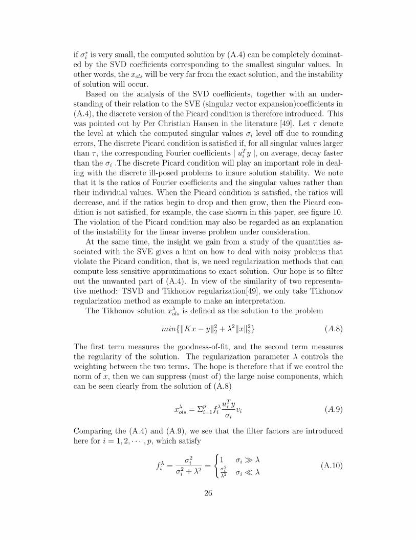
The Tikhonov solution xλols is defined as the solution to the problem
min∥Kx− y∥22 + λ2∥x∥22 (A.8)
The first term measures the goodness-of-fit, and the second term measuresthe regularity of the solution. The regularization parameter λ controls theweighting between the two terms. The hope is therefore that if we control thenorm of x, then we can suppress (most of) the large noise components, whichcan be seen clearly from the solution of (A.8)
xλols = Σpi=1f
λi
uTi y
σivi (A.9)
Comparing the (A.4) and (A.9), we see that the filter factors are introducedhere for i = 1, 2, · · · , p, which satisfy
fλi =
σ2i
σ2i + λ2
=
1 σi ≫ λσ2i
λ2 σi ≪ λ(A.10)
26

We stress here that the selection of λ is very crucial for the regularizationprocess. The method to determine it in the current paper is L-curve method.For the details, please see [47,48,49].
References
[1] Paul Arminjon, Claude Beauchamp, Numerical solution of Burgers’ equationsin two space dimensions,Computer Methods in Applied Mechanics and Engi-neering ,1979, 19 (3): 351-365.
[2] M. Basto, V. Semiao, F. Calheiros, Dynamics and synchronization of numericalsolutions of the Burgers equation, J. Comput. Appl. Math, 231(2009): 793-803.
[3] Bahadir, A.R., A fully implicit finite difference scheme for two-dimensionalBurgers equations, Appl. Math. Comput., 2003 137: 131-137.
[4] H.M.Park, Y.D.Jang, Control of Burgers equation by means of mode reduction,International Journal of Engineering Science, 2007, 38: 785-805.
[5] B. V. Rathish Kumar and Mani Mehra, A three-step wavelet Galerkin methodfor parabolic and hyperbolic partial differential equations, International Jour-nal of Computer Mathematics, 2006, 83(1): 143-157.
[6] Hongqing Zhu, Huazhong Shu and Meiyu Ding, Numerical solutions of two-dimensional Burgers’ equations by discrete Adomian decomposition method,Computers and Mathematics with Applications, 2010, (60): 840-848.
[7] P.Arminjon, C.Beauchamp, Numerical solution of Burgers equations in twospace dimensions,Comput. Meth. Appl. Mech. Eng., 1979, 19:351-365.
[8] C.A.J. Fletcher, Generating exact solutions of the two-dimensional Burgersequation, Int. J. Numer. Meth. Fluids, 1983 (3): 213C216.
[9] Nejib Smaoui, Boundary and distributed control of the viscous Burgers equa-tion, Journal of Computational and Applied Mathematics, 2005, 182: 91-104.
[10] H.M.Park, Y.D.Jang, Control of Burgers equation by means of mode reduc-tion,International Journal of Engineering Science, 2000, 38: 785-805.
[11] K. Kunisch, S. Volkwein, Control of the Burgers Equation by a Reduced- OrderApproach Using Proper Orthogonal Decomposition,Journal of OptimizationTheory and Applications, 1999, 102 (2): 345-371.
[12] Z. Wang, I. Akhtar, J. Borggaard, and T.Iliescu, Two-Level Discretizations ofNonlinear Closure Models for Proper Orthogonal Decomposition,J. Comput.Phys., 2011, 230: 126-146.
[13] Razvan Stefanescu, Adrian Sandu and Ionel M. Navon, Comparison of PODreduced order strategies for the nonlinear 2D shallow water equations, Int. J.Numer. Meth. Fluids, 2014, 76:497-521.
[14] F. Fang , C.C. Pain, I.M. Navon, M.D. Piggott, G.J. Gorman, P. Allison, A.J.H.Goddard, A POD reduced order unstructured mesh ocean modelling methodfor moderate Reynolds number flows, Ocean Modelling, 2009, 28: 127-136.
[15] S.Ravindran, A reduced-order approach for optimal control of fluids using prop-er orthogonal decomposition,Int. J. Numer. Meth. Fluids, 2000, 34: 425-448.
27

[16] S.Ravindran, Reduced-order adaptive controllers for fluid flows usingPOD,J.Sci, Comput., 2000, 15(4): 457-478.
[17] Loeve M., Probability Theory. Van Nostrand: Princeton, NJ, 1955.
[18] D.H.Chambers, R.J.Adrian, P.Moin, D.S.Stewart, and H.J.Sung, Karhunen-Loeve expansion of Burgers model of turbulence,Phys. Fluid, 1988; 31 (9):2573-2582.
[19] Hotelling H. Analysis of a complex of statistical variables with principal com-ponents. Journal of Educational Psychology, 1933; 24:417-441.
[20] Lorenz EN. Empirical orthogonal functions and statistical weather prediction.Technical Report, Massachusetts Institute of Technology, Dept. of Meteorology:Cambridge, MA, 1956.
[21] R.C.Gonzalez, P.A. Wintz, Digital Image Processing, Addison-Wesley, Read-ing, MA, 1987.
[22] Chaturantabut S. Dimension Reduction for Unsteady Nonlinear Partial Differ-ential Equations via Empirical Interpolation Methods. Technical Report TR09-38, CAAM, Rice University: Houston, TX, 2008.
[23] Chaturantabut S, Sorensen DC. A state space error estimate for POD-DEIM nonlinear model reduction.SIAM Journal on Numerical Analysis, 2012;50(1):46-63.
[24] Chaturantabut S, Sorensen DC. Nonlinear model reduction via discrete empir-ical interpolation. SIAM Journal on Scientific Computing , 2010; 32(5):2737-2764.
[25] Barrault M, Maday Y, Nguyen NC, Patera AT. An empirical interpolationmethod: application to efficient reduced basis discretization of partial differen-tial equations.Comptes Rendus Mathematique, 2004; 339(9):667-672.
[26] Grepl MA, Patera AT. A posteriori error bounds for reduced-basis approxima-tions of parametrized parabolic partial differential equations. ESAIM: Mathe-matical Modelling and Numerical Analysis, 2005; 39(01):157-181.
[27] Rozza G, Huynh DBP, Patera AT. Reduced basis approximation and a posteri-ori error estimation for affinely parametrized elliptic coercive partial differentialequations.Archives of Computational Methods in Engineering, 2008;15(3):229-275.
[28] Z. Wang, “Reduced-order modeling of complex engineering and geophysicalflows: Analysis and computations,” Ph.D. dissertation, Dept. App. Mathemat-ics, Virginia Polytechnic Institute and State University, 2012.
[29] N. Aubry, W. Y. Lian, and E.S. Titi, Preserving symmetries in the prop-er orthogonal decomposition, SIAM Journal on Scientific Computing, 1993;14:483-505.
[30] M. Couplet, C. Basdevant, P. Sagaut, Calibrated reduced-order POD-Galerkinsystem for fluid flow modelling, Journal of Computational Physics, 2005, 207:192-220.
[31] M. Bergmann, C. H. Bruneau, A. Iollo, Enablers for robust POD model-s,Journal of Computational Physics, 2009, 228: 516-538.
[32] A. Iollo, S. Lanteri, J. Desideri, Stability Properties of POD-Galerkin Approxi-mations for the Compressible Navier-Stokes Equations, Theoret. Comput. Flu-id Dynamics, 2000, 13: 377-396.
28
[33] J. Du, I. M. Navon, J. L. Steward, A. K. Alekseev and Z. Luo, Reduced-order modeling based on POD of a parabolized Navier-Stokes equation modelI: forward model, Int. J. Numer. Meth. Fluids, 2012, 69: 710-730.
[34] Omer San and Traian Iliescu, Proper Orthogonal Decomposition Closure Mod-els for Fluid Flows:Burgers Equation, International Journal of Numerical Anal-ysis and Modeling Series B , 2013, 1 (1): 1-18.
[35] Laurent Perret, Erwan Collin and J. Delville, Polynomial identification of PODbased low-order dynamical system, Journal of Turbulence , 2006, 7( 17): 1-15.
[36] V.L. Kalb, A.E. Deane, An intrinsic stabilization scheme for proper orthogonaldecomposition based low-dimensional models, Phys. Fluids, 2007, 19: 054106.
[37] L.Cordier, B. Abou El Majd and J. Favier, Calibration of POD reduced-ordermodels using Tikhonov Regularization, Int. J. Numer. Meth. Fluids, 2010;63:269-296.
[38] Bernardo Galletti, Alessandro Bottaro, Charles-Henri Bruneau, Angelo Iollo,Accurate model reduction of transient and forced wakes,European Journal ofMechanics B/Fluids, 2007 (26) : 354-366.
[39] H.M.Park, Y.D.Jang, Control of Burgers equation by means of mode reduction,International Journal of Engineering Science, 2007, 38: 785-805.
[40] Mehmet Onder Efe, Hitay Ozbay, Low dimensional modelling and Dirichletboundary controller design for Burgers equation, Int. J. Control, 2004, 77(10): 895-906.
[41] Samir Sahyoun, Seddik M. Djouadi, Nonlinear Model Reduction Using SpaceVectors Clustering POD with Application to the Burgers Equation, 2014American Control Conference (ACC) June 4-6, 2014. Portland, Oregon, USA.
[42] H. Imtiaz and I. Akhtar, Closure in Reduced-Order Model of Burgers Equa-tion, Proceedings of 2015 12th International Bhurban Conference on AppliedSciences and Technology (IBCAST), Islamabad, Pakistan, 13-17th January,2015.
[43] Hung V. Ly, Hien T. Tran, Modeling and Control of Physical Processes UsingProper Orthogonal Decomposition, Mathematical and Computer Modelling,2001, 33 : 223-236
[44] Masaaki Sugihara, Seiji Fujino, Numerical Solutions of Burgers equation witha large Reynolds number, Reliable Computing, 1996, 2(2): 173-179.
[45] C.T.Kelley, Iterative Methods for Linear and Nonlinear Equations, SIAM,Philadelphia, 1995.
[46] Philip Holmes, John L. Lumley, Gahl Berkooz,Clarencew Rowley, Turbulence,Coherent Structures,Dynamical Systems and Symmetry (2nd edition), Cam-bridge University Press, 2012.
[47] Adrian Doicu, Thomas Trautmann, and Franz Schreier, Numerical Regular-ization for Atmospheric Inverse Problems, Springer-Verlag Berlin Heidelberg,2010.
[48] Hansen, Per Christian, Discrete inverse problems: insight and algorithms,SIAM, Philadelphia, 2010.
[49] Hansen, Per Christian, The discrete Picard condition for discrete ill-posed prob-lems, BIT, 1990, 30(4): 658-672.
29

[50] Hansen PC. Regularization tools: a Matlab package for analysis and solutionof discrete ill-posed problems. Numerical Algorithms, 1994, 6: 1-35.
30