29 estimation of the di usion tensor i: the basic...

29 Estimation of the di↵usion tensor I:

The Basic Approach

1

29.1 Introduction

In the previous chapter we found that spins di↵using through a bipolar gradient result in adiminution of the signal from that which would have been produced by an equal number ofstationary spins because the di↵using spins acquire a distribution of phases concommitant withtheir distribution of spatial locations, and thus the integration of the signal over all spins leadsto incoherent averaging of the signal. Stationary spins, on the other hand, are refocussed by thesecond lobe in the bipolar pair, forming a gradient echo. The signal loss of the di↵using spindepends upon their phase distribution which, in turn, depends on the spatial distribution ofspins along the gradient direction, and thus our model for the signal depends upon our modelfor the di↵usion. For the simple model of Gaussian di↵usion2, the resulting signal took a verysimple form of an exponential decay as a function of both the imaging parameters, encapsulatedin the b-value, and the di↵usion tensor D.In this chapter we turn to the question that is faced at the end of all such experiments: Given

the data and our knowledge about the data, how do we estimate the physical quantities ofinterest? The first question is, of course, “What are the physical quantities of interest?” In thecase of Gaussian di↵usion, the answer to this question appears to be easy, since there is a singlequantity, the di↵usion tensor D, that characterizes the di↵usion. And, indeed, give this model,that’s about all we can do. But, as we shall see in later chapters, for more complex models thisquestion is not so easy to answer. Even in the present case the simplicity is somewhat illusory. Forexample, if we are looking at di↵usion in white matter in a patient with multiple scleroris, whatis the relationship between the di↵usion tensor and, say, the breakdown of the myelin sheath?This central question about the relationship of the estimated parameters of our model to thetrue underlying tissue structure is worth keeping in mind as a reality check on the informationcontent of the images that we acquire. Given the complexity of a block of neural tissue withina voxel, it is clear that we must strike a balance between a model that is su�ciently descriptiveto provide useful information on some aspect of tissue structure, while not so complex that wecannot e�ciently acquire the data necessary to estimate the parameters.The focus of this chapter is just that of the previous chapter: a single, di↵usion weighted voxel

1 This chapter has several sections commented out. They may have useful stu↵, but they were, for the mostpart, confusing

2 Shouldn’t there be a law of large number argument for why gaussian di↵usion is a good model for lots ofdi↵using spins?

524 Estimation of the di↵usion tensor I: The Basic Approach

(Figure 25.1). And I will present the essential first step in DTI analyses - the estimation of thedi↵usion tensor D, within the much simpler discussion of di↵usion sensitivity in a single voxelpresented in the previous chapter. For that is all we need in order to discuss the estimationof D. Once we have estimated D, we will see that we can derive some interesting quantitiesthat will tell us about the tissue. Later, when we are concerned with more global aspects suchas fiber connections, it will be important to have considered the entire imaging process. Butfor now we will consider the signal from a single voxel without any imaging. The analysis willbe the same when we expand to include image acquisition. But it is important to understandthe centeral feature that makes this separation possible (at least in the ideal case): The bipolardi↵usion weighting gradient are invisible to stationary spins. Therefore the di↵usion weightinggradients and the imaging procedure can be decoupled in our discussion. In reality, things arenot so simple, as the imaging gradients produce di↵usion weighting that must be accounted for.We’ll leave this complication for a later chapter.

29.2 What’s the problem?

So here is the problem that we are faced with. We have a set of measurements of the di↵usionweighted voxel and from these measurements we want to estimate the di↵usion tensor D. Aswe have seen, the di↵erent measurements can be either at di↵erent di↵usion sensitivities (i.e.,di↵erent b-values) or along di↵erent directions, or both. Typically we will be interested in thevariations of the di↵usion with direction, since this will tell us something about the underly-ing geometry (i.e., tissue architecture) of the environment in which spins are di↵usion. But wehave also seen that estimating the di↵usion coe�cient (the 1D problem) from multiple b-valuemeasurements involves the non-trivial problem of estimating a parameter from an exponentiallydecaying signal. Surely the more complex di↵usion tensor must also involve this aspect as well,and be even more non-trivial. In other words, shouldn’t the estimation of D involved measure-ments along di↵erent directions and with multiple b-values? The answer is yes but it should benoted that historically, and even in the majority of present practices, this is not what is typicallydone. Rather, a single b-value is chosen and D is estimated from multiple angular measurementstaken at this single b-values. There is another obvious but very important thing to keep in mindhere: The measurements required to estimate D will depend on the structure of D, or ratherour model for its structure. The simple model of unrestricted Gaussian di↵usion where D is areal, symmetric 3⇥ 3 matrix requires less measurements than a more complicated D that arisesin voxels that have a mixture of di↵erent tissues (which we address in Chapter 33). But this isjust the point that we made in Chapter 12: Both the measurements and estimates depend onthe model.

29.3 Constructing the b-matrix

Our data model, and thus our estimation of D, depends upon the tensor product bD. Beforeconsidering specifically how to estimate D, we’re going to take a slight detour and first considerthe structure of bD. In the simple problem of estimating the di↵usion coe�cient we made multiplemeasurements at di↵erent b-values in order to map out the exponential decay.

29.3 Constructing the b-matrix 525

Now let’s consider the problem of estimating the di↵usion tensor D from a set of angularmeasurements. Our data model is

s(q, ⌧) = s

o

e

�bD + ⌘(q) (29.1)

with

bD =X

i

X

j

b

ij

D

ij

(29.2)

where the factor that multiplies D

ij

, the i, j’th element of the di↵usion tensor, is

b

ij

= qi

qj

⌧ (29.3)

where q = g� and ⌧ = � � �/3. The i’th gradient points in the direction of the unit vector ui

,so denoting g

i

⌘ |gi

|, the q-vectors can be written qi

= q

i

ui

where q

i

= g

i

� and thus Eqn 29.2can be written

bD = b

ij

D

ij

(29.4)

where

b

ij

= q

i

q

j

⌧ (29.5a)

D

ij

= ui

D

ij

uj

(29.5b)

The set of n measurement at di↵erent angles is of the form Eqn 29.1, where b

ij

is given byEqn 29.5, in full matrix form:

b =

0

@q

2

x

q

x

q

y

q

x

q

z

q

y

q

x

q

2

y

q

y

q

z

q

z

q

z

q

z

q

y

q

2

z

1

A⌧ (29.6)

and the di↵usion tensor D, in its most general form, is

D =

0

@D

xx

D

xy

D

xz

D

yx

D

yy

D

yz

D

zx

D

zy

D

zz

1

A (29.7)

Since this matrix is symmetric, i.e., D = Dt, we’ve colored the equivalent o↵-diagonal compo-nents the same color. (In addition, the components are real, i.e., D

ij

2 R, although we won’t usethat fact just quite yet.) Let’s write out explicitly what the components of bD in Eqn 29.2 fora single gradient direction:

1

⌧

X

i

X

j

b

ij

D

ij

= q

2

x

D

xx

+ q

x

q

y

D

xy

+ q

x

q

z

D

xz

+ q

y

q

x

D

yx

+ q

2

y

D

yy

+ q

y

q

z

D

yz

+ q

z

q

x

D

zx

+ q

z

q

y

D

zy

+ q

2

z

D

zz

= q

2

x

D

xx

+ 2qx

q

y

D

xy

+ 2qx

q

z

D

xz

+ q

2

y

D

yy

+ 2qy

q

z

D

yz

+ + q

2

z

D

zz

where we’ve used the fact that D is symmetric so we can collect o↵-diagonal terms. Recall thatthe symmetry of D in Eqn 29.7 derives from the physical property of our measurements that


the di↵usion related signal loss is the same whether the net motion is along the positive ornegative gradient direction3. If we visualize the di↵usion gradient direction as a line that goesfrom the origin to a point on the surface of the sampling sphere, then the signal loss due to thisgradient is the same if the gradient is applied in the opposite direction, which is represented bya line from the origin to a point directly on opposite sides of the sampling sphere, the so-calledantipodal points4. This symmetric is therefore called antipodal symmetry . The result is that theo↵-diagonal terms are equal.Now, a trick is usually pulled here in practice (?) is to note that

s

o

e

�bD = e

log(s

o

)

e

�bD = e

�bD+log(s

o

) = e

�Bd+log(s

o

) (29.8)

Therefore, if we define a vector

Bt =�q

2

x

, q

2

y

, q

2

z

, q

x

q

y

, q

x

q

z

, q

y

q

z

, 1�⌧ (29.9)

and

dt = (Dxx

, D

yy

, D

zz

, D

xy

, D

xz

, D

yz

, � log s

o

) (29.10)

and so the equation for our data looks like

s(b) = exp��Btd

�+ ⌘ (29.11)

This form is nice because it involves only two quantities, B which are the known gradientdirections, and d which are the elements of the di↵usion tensor we want to estimate. However,there are 7 unknowns in d, so we need 7 equations to solve for them all. To do this, we need toacquire 7 di↵erent measurements. If all the measurements were pointing in the same directions,this would add no new information to the problem. So we need to acquire measurements at

di↵erent directions. If we gather n directions, each produces a product of the form Bt

k

d k =1, . . . , n, so we can describe the whole problem by constructing a matrix where each B

k

of theform Eqn 29.9 are the di↵erent rows

0

BBB@

s(b1

)s(b

2

)...

s(bn

)

1

CCCA

| {z }y

= exp

2

666666664

�

0

BBB@

Bt

1

Bt

2

...Bt

n

1

CCCA

| {z }B

d

3

777777775

+

0

BBB@

⌘(b1

)⌘(b

2

)...

⌘(bn

)

1

CCCA

| {z }⌘

(29.12)

where B is called the b-matrix (?). Writing it out in full, it is

B =

0

BBB@

q

2

1,x

q

2

1,y

q

2

1,z

q

1,x

q

1,y

q

1,x

q

1,z

q

1,y

q

1,z

1q

2

2,x

q

2

2,y

q

2

2,z

q

2,x

q

2,y

q

2,x

q

2,z

q

2,y

q

2,z

1...

q

2

n,x

q

2

n,y

q

2

n,z

q

n,x

q

n,y

q

n,x

q

n,z

q

n,y

q

n,z

1

1

CCCA⌧ (29.13)

3 True?!4 put earlier in the discussion of gradient directions! in dti-sensit. Show picture!

29.4 Estimation of the di↵usion tensor D: Angular sampling 527

Alternatively, under ideal conditions in which the gradients are perfect, Eqn 29.13 can be rewrit-ten in terms of the directional vector q = qu, where q = |q|.

B = b

0

BBB@

u

2

1,x

u

2

1,y

u

2

1,z

u

1,x

u

1,y

u

1,x

u

1,z

u

1,y

u

1,z

1/b

u

2

2,x

u

2

2,y

u

2

2,z

u

2,x

u

2,y

u

2,x

u

2,z

u

2,y

u

2,z

1/b

...u

2

n,x

u

2

n,y

u

2

n,z

u

n,x

u

n,y

u

n,x

u

n,z

u

n,y

u

n,z

1/b

1

CCCA(29.14)

where b = q

2

⌧ and q = g� and ⌧ = (�� /3).In practice (i.e., in an actual scanner), the full matrix B is calculated by incorporating the

actual true waveforms on the scan (which might have slight variations from ideality) and, if oneis being careful, the di↵usion weighting e↵ects of the imaging gradients. But Eqn 29.14 is usefulin understanding the influence of gradient direction choices.It is useful to recall at this point the relationship between the matrix B and what is going

on in the scanner. Recall that a single di↵usion weighted direction is created by a combinationof bipolar gradients along the three axes, as shown in Figure 29.1. The multiple measurementsare made by suitable combinations of the gradients for producing di↵usion weighting directionsthat are isotropically distributed on a spherical surface (by various methods, as discussed inSection 29.9 below). From these are determined the matrix B.

29.4 Estimation of the di↵usion tensor D: Angular sampling

We have thus reduced the problem of estimating the di↵usion tensor to finding the solution tothe matrix equation

y = exp [�Bd] + ⌘ (29.15)

where

y = [n ⇥ 1] , data

B = [n ⇥ m] , B-matrix

d = [m ⇥ 1] , (so

, and components of D)

If there were no noise, we could just take the log of both sides of Eqn 29.15 to get � log(y) = Bdand solving this by linear least squares (?). However, this approach is incorrect because the model(no noise) is incorrect (?): least squares assumes that the noise is additive and each sample has thesame variance. Both of these assumptions are violated when the logarithm is taken. In addition,the D estimated from the log of the data is not guaranteed to have positive eigenvalues. 5

Rather, it is best to directly fit the data to the model. This can be accomplished using anynumber of fitting routines which are widely available, including in such standard platforms atMATLAB (?) and Mathematica (?). However, even fitting the model directly does not guaranteenegative eigenvalues. Therefore, a fitting routine that also incorporates the constraint of positiveeigenvalues is important in getting physically meaningful result. One such method (that we use inmy lab) is that due to Cox (?), which is distributed in the AFNI package (?). This is a non-linearmethod that uses a gradient descent algorithm modified so that the estimated di↵usion tensor

5 More explanation here? Should have this discussion somewhere.


t

Gx

t

Gy

t

Gz

(a) Gradients (b) Di↵usion weighting direction.

Figure 29.1 An example of gradients for a single di↵usion encoding direction. The e↵ects of gradients

add like vectors so the direction and amplitude of the applied di↵usion weighting gradient is defined by

the vector sum of the gradients. The e↵ect of gradients only along the x, y, or z axes is shown in (a-c),

red, green, blue, respectively. With all gradients turned on simultaneously at di↵erent amplitudes

produces and direction that is the vector sum (yellow).

remains positive definite (and thus has positive eigenvalues Section 8.12). Results of this methodin comparison with the log-linear method are shown in Figure 29.2.6

29.5 Eigenvectors and eigenvalues of the di↵usion tensor

As we saw in Chapter 24, the di↵usion tensor D is symmetric and its elements are real. Thesetwo facts are expressed mathematically as:

D = Dt or D

ij

= D

ji

, symmetric matrix (29.16)

D

ij

2 R , real matrix (29.17)

But from our discussion in Section 8.6 we can restate the spectral theorem in more practicalterms: The di↵usion tensor D is a real, symmetric matrix and therefore can be rotated to make

it diagonal. That is, there exists some 3D rotation matrix R for which the matrix D (Eqn 29.7)

6 This shows an image and so should be in dti-basic.tex where we first show images!

29.5 Eigenvectors and eigenvalues of the di↵usion tensor 529

(a) Fitting the log-linear model produces spu-rious FA values (> 1) because D is no longerassured to be positive definite.

(b) Directly fitting the exponential form ofthe signal allows constraining D to be positivedefinite and consequently that 0 FA 1.

Figure 29.2 Estimation of the di↵usion tensor using the method of Cox (?) to directly fit the

exponential decay. Shown is the fractional anisotropy.

can be transformed into a diagonal form D⇤

:

D⇤

= RtDR = RtR =

0

@�

1

0 00 �

2

00 0 �

3

1

A (29.18)

In practice, this procedure of diagonalization is done numerically by specialized algorithms de-signed specifically for this procedure.

We can now return to the results of Section 27.2 where we found that for free di↵usion theprobability distribution of the spins is given by Eqn 27.1

p(r, ⌧) =1p

|D| (4⇡⌧)3exp

⇥�rtD�1r/(4⌧)

⇤(29.19)

where r is the mean displacement vector and ⌧ = � � �/3. This distribution describes thespin displacement during the di↵usion measurement period, |.| is the determinant and D isthe di↵usion tensor. This is a multivariate Gaussian distribution with covariance matrix 2⌧D.The covariance matrix determines the width of the distribution and thus describes how much thespins have ”spread out” during the measurement time. But we studied the multivariate Gaussianin-depth in Section 8.7 and we can now use those results.

So for a tissue where the di↵usion varies as a function of direction, the distribution of describedby the multivariate Gaussian of Eqn 8.48, with the variance �

2

i

= 2Di

⌧ where i = {x, y, z}. In


other words, the covariance matrix is

M =

0

@2D

x

⌧ 0 00 2D

y

⌧ 00 0 2D

z

⌧

1

A (29.20)

where the eigenvalues are

�

1

= 2Dx

⌧ , �

2

= 2Dy

⌧ , �

3

= 2Dz

⌧ (29.21)

Because of the common constant factor of 2⌧ in these equations, it is more e�cient to write thecovariance matrix as M = 2⌧D where

D⇤

=

0

@�

1

0 00 �

2

00 0 �

3

1

A (29.22)

where D⇤

is called the di↵usion tensor and has eigenvalues

{�1

, �

2

, �

3

} = {Dx

, D

y

, D

z

} (29.23)

Note that, because the di↵usion coe�cients are related to the variances, which are inverselyproportional to the eigenvalues, that they are thus linearly related to the eigenvalues. That is,the eigenvalues are the di↵usion coe�cients! Again, this is the covariance matrix structure if thevariance directions - i.e., the di↵usion coe�cients directions - are aligned with the coordinate(spatial) axes {x, y, z}. If they are not, then the covariance matrix is not diagonal. But, again,we can make it so, and thus determine the eigenvalues and eigevectors, which in turn gives usthe di↵usion coe�cients and the directions of di↵usion. The orientation of the di↵usion tensorrelative to the magnet coordinates depends upon the orientation of the tissue relative to thesecoordinates, and in generate is rotated. The di↵usion tensor in the frame in which it is diagonal(the tissue frame) is related to the magnet frame by the similarity transform we discussed inSection 8.5. The di↵usion tensor is thus (Eqn 27.14)

D ⌘ Rt D⇤

R (29.24)

The situation is just as we discussed in Section 8.7: the contours of probability for the multivariateGaussian di↵usion are ellipsoids, as shown in Figure 29.3.

29.6 The average eigenvalue: the mean di↵usivity

A natural question to ask is “What is the average di↵usion D in the voxel?” where D is given,generally, by Eqn 29.7. Well, how do you take the average of this? Let’s first look at D in thecoordinate system in which it is diagonal, that is, in the eigencoordinates of D. Here the averageis easy:

hDi = 1

3(D

e1,e1 + D

e2,e2 + D

e3,e3) =1

3(�

1

+ �

2

+ �

3

) =1

3Tr(D) (29.25)

where we’ve used the fact that the trace Tr(.) of a matrix is (Section 5.6) is the sum of thediagonal elements of the matrix. Therefore Tr(D) is a measure of the total di↵usion in a voxeland 1

3

Tr(D) is the average over the di↵erent directions of the eigenvectors, and is called the mean

di↵usivity . Since each measurement provides an estimate of the apparent di↵usion coe�cient or

29.6 The average eigenvalue: the mean di↵usivity 531

Figure 29.3 Estimation of the di↵usion tensor eigenvalues and eigenvectors allows reconstruction of the

Gaussian probability distribution whose contours of equal probability are ellipsoidal. The principle axes

of the ellipsoid are the eigenvectors of the di↵usion tensor. The lengths of the eigenvectors are

proportional to the square-root of the di↵usion tensor eigenvalues � times the di↵usion time ⌧ .

ADC along that direction, the hDi is the average ADC. When we say “average”, we really needto be more specific and say “average over directions”. Charaterizing these directions as di↵erentangles ⌦ ⌘ {#, '}, we should write hDi

⌦

which symbolizes that the average is over the values of⌦ at which the measurements were taken.

Now let’s return to our original problem of determining hDi for D given by Eqn 29.7, whichis related to D

⇤

by Eqn 29.24. But now recall (Eqn 8.43) the invariance of the trace to cyclicpermutation of the elements:

Tr(D) = Tr(R⇤Rt) = Tr(RtR⇤) = Tr(⇤) (29.26)

and the fact that rotation matrices are orthonormal (Section 5.16): RtR = 1, so that

Tr(D) = Tr(⇤) =3X

i=1

�

i

= 3� (29.27)

where � = 1

3

P3

i=1

�

i

is the average eigenvalue. This tells us mathematically what you had prob-ably already guessed - the average di↵usion should not change just because we changed theorientation of the probability distribution. But it also tells us something that is useful computa-tionally: The trace of D of the form Eqn 29.7 is the same as the trace of D

⇤

in its diagonal form.So it is not necessary to diagonalize the matrix in order to determine the trace - you just sumthe elements along the diagonal and it works out the same! This scalar quantity hDi is invariantto orientation and thus is called a scalar invariant .

An intuitive picture of what is happening physically is provided by a simple geometrical depic-tion. Denoting ��

i

= �

i

� �, the di↵erence of the i’th eigenvalue from the mean, we can rewrite


Eqn 29.22 in the form

D⇤

=

0

@� 0 00 � 00 0 �

1

A

| {z }D

+

0

@��

1

0 00 ��

2

00 0 ��

3

1

A

| {z }�D

(29.28)

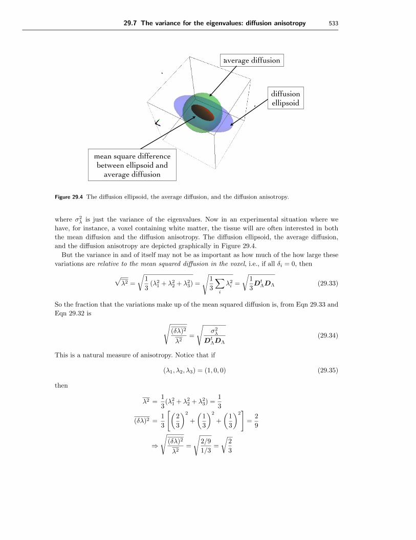
where we’ve used the fact (Section 5.3) that we can write a matrix as the sum of other matrices.We’ve now written D in terms of a diagonal matrix D where all the diagonal elements are equaland another diagonal matrix �D where the elements are the deviations from the mean �. Buta diagonal matrix with all the elements equal has the geometrical representation of a sphere -the eigenvectors are all of the same length. This means that the contour of constant probabilityare spherical, as shown in Figure 29.4. This represents the average di↵usion over the di↵erentdirections and is independent of orientation. Recall from our discussion in Section 8.5 that thetrace is invariant to rotations of the matrix so that

Tr(D) =

0

@D

xx

D

xy

D

xz

D

yx

D

yy

D

yz

D

zx

D

zy

D

zz

1

A

| {z }D

xx

+ D

yy

+ D

zz

=

0

@�

x

0 00 �

y

00 0 �

z

1

A

| {z }�

x

+ �

y

+ �

z

(29.29)

29.7 The variance for the eigenvalues: di↵usion anisotropy

The matrix �D contains the deviations of the eigenvalues from their average value, and thus isrelated to the di↵erences between the di↵usion along the principle axes. If there we no variations,i.e., ��

1

= ��

2

= ��

3

= 0, then the di↵usion is the same in all directions and is said to be isotropic.But if any of the ��

i

are di↵erent, then the di↵usion is not equal along all directions, and is saidto be anisotropic. A natural way to characterize these di↵erences is to look at the variance ofthe eigenvalues. We can rearrange Eqn 29.28 to write the matrix of deviations as

�D =

0

@��

1

0 00 ��

2

00 0 ��

3

1

A =

0

@�

1

� � 0 00 �

2

� � 00 0 �

3

� �

1

A (29.30)

Now these deviations ��

i

can be either positive or negative, depending upon whether the partic-ular eigenvalue is greater than or less than the mean. But if we are only interested in how muchour shape deviates from a sphere, that is, how much our di↵usion deviates from isotropic, we onlycare about the magnitude of the di↵erence. So what the average magnitude of the deviation?Well, this is just

q(��)2 =

vuut1

3

3X

i=1

��

2

i

(29.31)

But this is just

q(��)2 =

r1

3�Dt

�D =

r1

3

⇥(�

1

� �)2 + (�2

� �)2 + (�3

� �)2⇤=

r1

3�

2

�

(29.32)

29.7 The variance for the eigenvalues: di↵usion anisotropy 533

⌧

diffusion ellipsoid

average diffusion

mean square difference between ellipsoid and

average diffusion

Figure 29.4 The di↵usion ellipsoid, the average di↵usion, and the di↵usion anisotropy.

where �

2

�

is just the variance of the eigenvalues. Now in an experimental situation where wehave, for instance, a voxel containing white matter, the tissue will are often interested in boththe mean di↵usion and the di↵usion anisotropy. The di↵usion ellipsoid, the average di↵usion,and the di↵usion anisotropy are depicted graphically in Figure 29.4.But the variance in and of itself may not be as important as how much of the how large these

variations are relative to the mean squared di↵usion in the voxel, i.e., if all �

i

= 0, then

p�

2 =

r1

3(�2

1

+ �

2

2

+ �

2

3

) =

s1

3

X

i

�

2

i

=

r1

3Dt

⇤

D⇤

(29.33)

So the fraction that the variations make up of the mean squared di↵usion is, from Eqn 29.33 andEqn 29.32 is

s(��)2

�

2

=

s�

2

�

Dt

⇤

D⇤

(29.34)

This is a natural measure of anisotropy. Notice that if

(�1

, �

2

, �

3

) = (1, 0, 0) (29.35)

then

�

2 =1

3(�2

1

+ �

2

2

+ �

2

3

) =1

3

(��)2 =1

3

"✓2

3

◆2

+

✓1

3

◆2

+

✓1

3

◆2

#=

2

9

)

s(��)2

�

2

=

s2/9

1/3=

r2

3


(a) Oblate. �1 = �2 � �3 (b) Prolate. �1 � �2 ⇡ �3 (c) Spherical. �1 ⇡ �2 ⇡ �3

Figure 29.5 Di↵usion ellipsoid shape classifications for special cases of eigenvalue combinations.

So normalizing Eqn 29.34 so that the maximum value is 1 we can define

FA =

s3

2

(��)2

�

2

, Fractional anisotropy (29.36)

Eqn 29.36 is called the fractional anisotropy or FA. It is the most common index of anisotropyused in practice. 7. It is quite remarkable that this rather straightforward calculation gives whatappears to be a remarkably good image of the white matter! 8

29.8 Other Anisotropy Measures

There are some practical cases in which there are two (nearly) equal eigenvalues, in which casethere is a nice shape description for the di↵usion ellipsoid in terms of oblate and prolate ellipsoids,as shown in Figure 29.5. Sometimes these shapes are called linear and planar rather than prolateand oblate, respectively. These three shapes can be characterized by the following anisotropyindeces (?):

linear : c

l

=�

1

� �

2

3�(29.37a)

planar : c

p

=2(�

2

� �

3

)

3�(29.37b)

spherical : c

s

=�

3

�

(29.37c)

where

� ⌘ 1

3(�

1

+ �

2

+ �

3

) (29.38)

is the average eigenvalue.

7 Show a single voxel example here!8 Check all the FA stu↵ for the constants!

29.9 How do we choose our angular sampling? 535

29.9 How do we choose our angular sampling?

In Section 29.4 we noted that we need at least 7 measurements to estimate the six uniquecomponents of D plus the normalizing factor s

o

. But what 7 measurements? And is 7 reallyenough? And what do we mean by “enough”? 9 For angular measurements where b is a matrix,it is required that b1 is invertible. As we discussed at length in Eqn 5.12, in order for a matrix tobe invertible, there are certain restrictions on the relationship amongst the column vectors thatcompose it. In particular, they must be linearly independent (CHECK!). This means that noneof the vectors can be colinear with any of the other vectors. In other words, the vectors must be

non-colinear. That is, they must all point in di↵erent directions. But is that enough? Intuitively,you could imagine that sampling n non-colinear directions that lie on the surface of a cone witha very angle10 is not taking measurements in directions that are very di↵erent, and so must havetrouble detecting the ellipsoidal variations in the MR signal as a function of angle. How do wequantify this intuitive concept?

The answer to this question was found in our discussion of the amplitude estimates in ourmatrix formulation of the parameter estimation problem in probability theory (Section 12.9).The amplitude estimates depend on the pseudo-inverse, which we found in Eqn 12.97. For the3-dimensional problem here, this means that there are 3 non-zero eigenvalues of the the pseudo-inverse of the b-matrix, b(�1) = (btb)�1bt. The angular spacing of the samples decides the relativeweighting of these eigenvalues. In order for our estimates to be equally weighted, we want theseeigenvalues to be approximately equal. This is equivalent to having the samples isotropicallydistributed about the sphere 11. This is shown in Figure 34.7 where we compare the tesselationmethod (Figure 34.7a), which produces essentially an equi-angular distribution, with a randomdistribution of angles (Figure 34.7b). Note that the equi-angular distribution produces a strongdiagonal component in the pseudo-inverse matrix. This, then, conforms with our intuition: wewant samples that are equally spaced on a sphere.

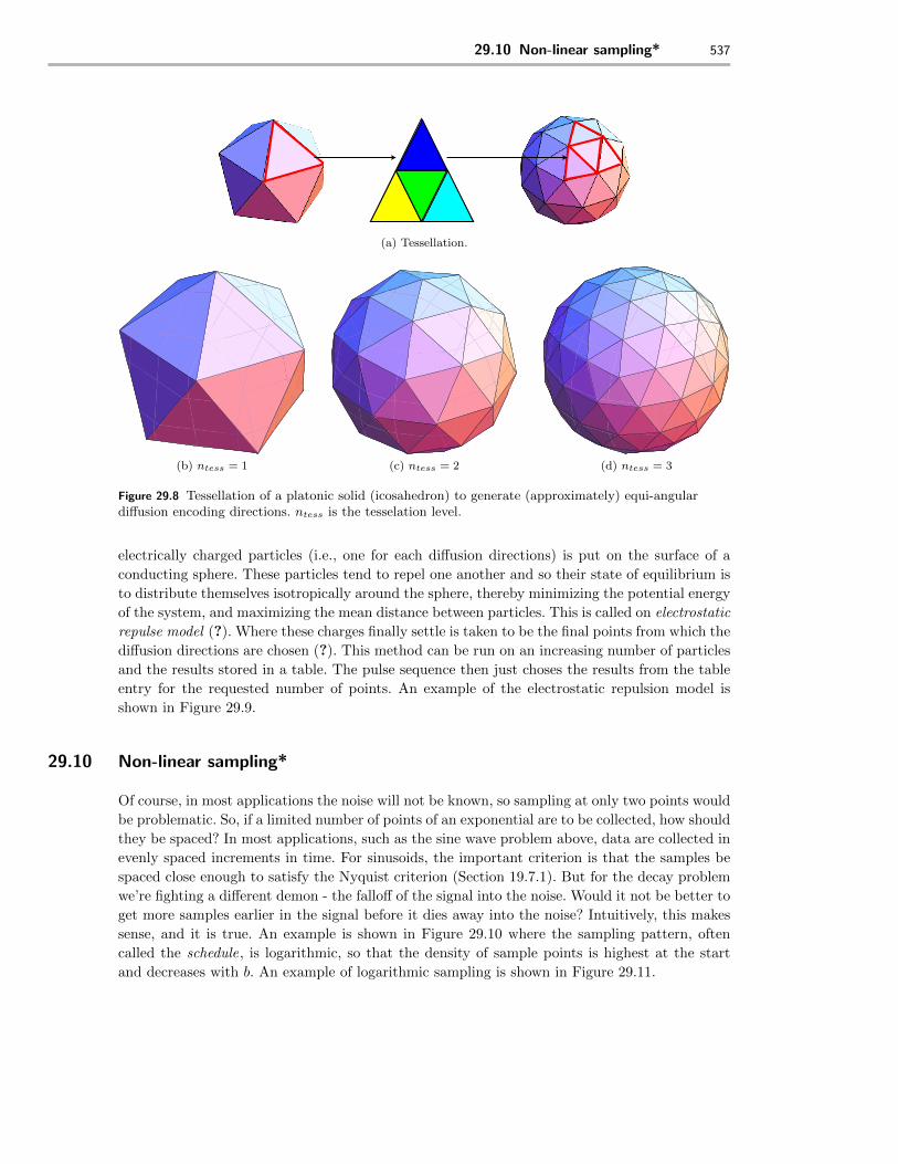
Having decided that we want samples equally distributed on a sphere, how can this be achievednumerically? One common method, illustrated in Figure 29.7, is to use the vertices of a platonicsolid. These vertices are well known and can be easily programmed into the pulse sequencesoftware. One limitation of this method, however, is that the platonic solids do not have manyvertices. As we shall see in later chapters, it is often necessary to collect many di↵erent directions(say, 64). However, there is a nice way to extend the platonic sampling method to more directions.Each “face” of the solid, defined by the flat surface between the vertices, is cut up into smallerversions of the same shape by cutting the lines between the vertices in half. This process is calledtessellation, and is illustrated for triangular faces in Figure 29.8a. This process can be repeatedad infinitum on the new, smaller faces. An example of a tessellated icosahedron is shown inFigure ??. However, this method still has a major limitation: For any given platonic solid, thereare only a discrete set of directions available, since the tesselation procedure produces a fixednumber of additional vertices. For example, in Figure 29.8a we see that each triangular facedefined by 3 vertices becomes 4 faces with 6 unique vertices. Moreover, the number of verticesgrows very rapidly, since this procedure takes place at every face, generated more faces, eachwhich then gets tessellated again. For example, the icosahedron in Figure ?? has 12 vertices, and

9 Haven’t discussed total number of samples yet!10 what is that cone angle called?11 Why?!


-1.0

-0.5

0.0

0.5

1.0

-1.0

-0.5

0.0

0.5

1.0

-1.0

-0.5

0.0

0.5

1.0

5 10 15

0.05

0.10

0.15

(a) Approximately equally spaced angularly through tesselation. (left) Sampling; (center)b-matrix; (right) eigenvalue spectrum of b-matrix.

-1.0

-0.5

0.0

0.5

1.0

-1.0

-0.5

0.0

0.5

1.0

-1.0

-0.5

0.0

0.5

1.0

5 10 15

0.1

0.2

0.3

0.4

(b) Randomly spaced. (left) Sampling; (center) b-matrix; (right) eigenvalue spectrum ofb-matrix.

Figure 29.6 Eigenvalues of b(�1)= (btb)�1bt, the pseudo-inverse of the b-matrix. (Say something

about eigenvalue spectra!)

Figure 29.7 Isotropically distributed di↵usion directions samples chosen as the vertices of a platonic

solid (an icosahedron).

on subsequent levels of tessellation produces {42, 162, 642, 2562} vertices. In a standard imagingprotocol a “large” number of directions is around 60, which means that only the second level oftesselation (i.e., 42 vertices) is allowed. Thus the tesselation method is quite restrictive in whatdirections it produces.

An alternative strategy that allows an essentially arbitrary number of equally points on asphere to be generated is to utilize what is a numerical method wherein a desired number of

29.10 Non-linear sampling* 537

⌧

(a) Tessellation.

(b) ntess = 1 (c) ntess = 2 (d) ntess = 3

Figure 29.8 Tessellation of a platonic solid (icosahedron) to generate (approximately) equi-angular

di↵usion encoding directions. ntess is the tesselation level.

electrically charged particles (i.e., one for each di↵usion directions) is put on the surface of aconducting sphere. These particles tend to repel one another and so their state of equilibrium isto distribute themselves isotropically around the sphere, thereby minimizing the potential energyof the system, and maximizing the mean distance between particles. This is called on electrostatic

repulse model (?). Where these charges finally settle is taken to be the final points from which thedi↵usion directions are chosen (?). This method can be run on an increasing number of particlesand the results stored in a table. The pulse sequence then just choses the results from the tableentry for the requested number of points. An example of the electrostatic repulsion model isshown in Figure 29.9.

29.10 Non-linear sampling*

Of course, in most applications the noise will not be known, so sampling at only two points wouldbe problematic. So, if a limited number of points of an exponential are to be collected, how shouldthey be spaced? In most applications, such as the sine wave problem above, data are collected inevenly spaced increments in time. For sinusoids, the important criterion is that the samples bespaced close enough to satisfy the Nyquist criterion (Section 19.7.1). But for the decay problemwe’re fighting a di↵erent demon - the fallo↵ of the signal into the noise. Would it not be better toget more samples earlier in the signal before it dies away into the noise? Intuitively, this makessense, and it is true. An example is shown in Figure 29.10 where the sampling pattern, oftencalled the schedule, is logarithmic, so that the density of sample points is highest at the startand decreases with b. An example of logarithmic sampling is shown in Figure 29.11.


(a) Di↵usion directions gener-ated from the origin to thepoints in (a).

(b) Points on a sphere gener-ated by the electrostatic repul-sion model

Figure 29.9 The electrostatic repulse model. Points are chosen so as to minimize the energy of charged

points on a sphere.

20 40 60 80 100sample

200

400

600

800

1000

b

(a) Linear sampling of b.

20 40 60 80 100 sample

200

400

600

800

1000b

(b) Logarithmic sampling of b.

Figure 29.10 The default strategy for sampling is usually equally spaced samples, as in (a). For the

decay problem, however, a higher sampling density during the initial part of the signal allows the

acquisition of more data with high SNR than equally spaced samples.

Suggested reading

29.10 Non-linear sampling* 539

100 200 300 400 500

20

40

60

80

(a) {A, d} = {98.5, .00510}100 200 300 400 500

20

40

60

80

100

(b) {A, d} = {101.9, .0498}100 200 300 400 500

20

40

60

80

100

(c) {A, d} = {98.1, .0055}

100 200 300 400 500

-40

-20

0

20

40

(d) residual = 1.69

100 200 300 400 500

-40

-20

0

20

40

(e) residual = 2.03

100 200 300 400 500

-40

-20

0

20

40

(f) residual = 2.44

Figure 29.11 Logarithmic sampling of the exponential decay for fixed SNR = 10 decay rate d = .050 as

a function of the number os samples. The amplitude is A = 100. Reasonable estimates are possible even

with very few samples.

29 estimation of the di usion tensor i: the basic...

Documents