22392033 numerical methods course notes
TRANSCRIPT

Numerical Methods Course Notes
Version 0.11
(UCSD Math 174, Fall 2004)
Steven E. Pav1
October 13, 2005
1Department of Mathematics, MC0112, University of California at San Diego, La Jolla, CA 92093-0112.<[email protected]> This document is Copyright c© 2004 Steven E. Pav. Permission is granted to copy,distribute and/or modify this document under the terms of the GNU Free Documentation License, Version1.2 or any later version published by the Free Software Foundation; with no Invariant Sections, no Front-Cover Texts, and no Back-Cover Texts. A copy of the license is included in the section entitled ”GNU FreeDocumentation License”.

2

Preface
These notes were originally prepared during Fall quarter 2003 for UCSD Math 174, NumericalMethods. In writing these notes, it was not my intention to add to the glut of Numerical Analysistexts; they were designed to complement the course text, Numerical Mathematics and Computing,
Fourth edition, by Cheney and Kincaid [7]. As such, these notes follow the conventions of thattext fairly closely. If you are at all serious about pursuing study of Numerical Analysis, you shouldconsider acquiring that text, or any one of a number of other fine texts by e.g., Epperson, Hamming,etc. [3, 4, 5].
3.1
3.2 8.4
3.3
1.4
3.4
1.1
4.2 7.1 10.1
4.3
5.1
5.2
7.2
8.3
8.2
9.1
9.2 9.3
10.2
10.3
Figure 1: The chapter dependency of this text, though some dependencies are weak.
Special thanks go to the students of Math 174, 2003–2004, who suffered through early versionsof these notes, which were riddled with (more) errors.
Revision History
0.0 Transcription of course notes for Math 174, Fall 2003.0.1 As used in Math 174, Fall 2004.
0.11 Added material on functional analysis and Orthogonal Least Squares.
Todo
• More homework questions and example problems.• Chapter on optimization.• Chapters on basic finite difference and finite element methods?• Section on root finding for functions of more than one variable.
i

ii

Contents
Preface i
1 Introduction 1
1.1 Taylor’s Theorem . . . . . . . . . . . . . . . . . . . . . . . . . . . . . . . . . . . . . . 1
1.2 Loss of Significance . . . . . . . . . . . . . . . . . . . . . . . . . . . . . . . . . . . . . 4
1.3 Vector Spaces, Inner Products, Norms . . . . . . . . . . . . . . . . . . . . . . . . . . 5
1.3.1 Vector Space . . . . . . . . . . . . . . . . . . . . . . . . . . . . . . . . . . . . 5
1.3.2 Inner Products . . . . . . . . . . . . . . . . . . . . . . . . . . . . . . . . . . . 6
1.3.3 Norms . . . . . . . . . . . . . . . . . . . . . . . . . . . . . . . . . . . . . . . . 7
1.4 Eigenvalues . . . . . . . . . . . . . . . . . . . . . . . . . . . . . . . . . . . . . . . . . 8
1.4.1 Matrix Norms . . . . . . . . . . . . . . . . . . . . . . . . . . . . . . . . . . . . 8
Exercises . . . . . . . . . . . . . . . . . . . . . . . . . . . . . . . . . . . . . . . . . . . . . 10
2 A “Crash” Course in octave/Matlab 13
2.1 Getting Started . . . . . . . . . . . . . . . . . . . . . . . . . . . . . . . . . . . . . . . 13
2.2 Useful Commands . . . . . . . . . . . . . . . . . . . . . . . . . . . . . . . . . . . . . 17
2.3 Programming and Control . . . . . . . . . . . . . . . . . . . . . . . . . . . . . . . . . 19
2.3.1 Logical Forks and Control . . . . . . . . . . . . . . . . . . . . . . . . . . . . . 20
2.4 Plotting . . . . . . . . . . . . . . . . . . . . . . . . . . . . . . . . . . . . . . . . . . . 21
Exercises . . . . . . . . . . . . . . . . . . . . . . . . . . . . . . . . . . . . . . . . . . . . . 24
3 Solving Linear Systems 25
3.1 Gaussian Elimination with Naıve Pivoting . . . . . . . . . . . . . . . . . . . . . . . . 25
3.1.1 Elementary Row Operations . . . . . . . . . . . . . . . . . . . . . . . . . . . . 25
3.1.2 Algorithm Terminology . . . . . . . . . . . . . . . . . . . . . . . . . . . . . . 27
3.1.3 Algorithm Problems . . . . . . . . . . . . . . . . . . . . . . . . . . . . . . . . 28
3.2 Pivoting Strategies for Gaussian Elimination . . . . . . . . . . . . . . . . . . . . . . 29
3.2.1 Scaled Partial Pivoting . . . . . . . . . . . . . . . . . . . . . . . . . . . . . . 30
3.2.2 An Example . . . . . . . . . . . . . . . . . . . . . . . . . . . . . . . . . . . . 31
3.2.3 Another Example and A Real Algorithm . . . . . . . . . . . . . . . . . . . . . 32
3.3 LU Factorization . . . . . . . . . . . . . . . . . . . . . . . . . . . . . . . . . . . . . . 33
3.3.1 An Example . . . . . . . . . . . . . . . . . . . . . . . . . . . . . . . . . . . . 34
3.3.2 Using LU Factorizations . . . . . . . . . . . . . . . . . . . . . . . . . . . . . . 36
3.3.3 Some Theory . . . . . . . . . . . . . . . . . . . . . . . . . . . . . . . . . . . . 37
3.3.4 Computing Inverses . . . . . . . . . . . . . . . . . . . . . . . . . . . . . . . . 37
3.4 Iterative Solutions . . . . . . . . . . . . . . . . . . . . . . . . . . . . . . . . . . . . . 37
3.4.1 An Operation Count for Gaussian Elimination . . . . . . . . . . . . . . . . . 37
iii

iv CONTENTS
3.4.2 Dividing by Multiplying . . . . . . . . . . . . . . . . . . . . . . . . . . . . . . 39
3.4.3 Impossible Iteration . . . . . . . . . . . . . . . . . . . . . . . . . . . . . . . . 40
3.4.4 Richardson Iteration . . . . . . . . . . . . . . . . . . . . . . . . . . . . . . . . 40
3.4.5 Jacobi Iteration . . . . . . . . . . . . . . . . . . . . . . . . . . . . . . . . . . . 41
3.4.6 Gauss Seidel Iteration . . . . . . . . . . . . . . . . . . . . . . . . . . . . . . . 42
3.4.7 Error Analysis . . . . . . . . . . . . . . . . . . . . . . . . . . . . . . . . . . . 42
3.4.8 A Free Lunch? . . . . . . . . . . . . . . . . . . . . . . . . . . . . . . . . . . . 44
Exercises . . . . . . . . . . . . . . . . . . . . . . . . . . . . . . . . . . . . . . . . . . . . . 46
4 Finding Roots 49
4.1 Bisection . . . . . . . . . . . . . . . . . . . . . . . . . . . . . . . . . . . . . . . . . . 49
4.1.1 Modifications . . . . . . . . . . . . . . . . . . . . . . . . . . . . . . . . . . . . 49
4.1.2 Convergence . . . . . . . . . . . . . . . . . . . . . . . . . . . . . . . . . . . . 50
4.2 Newton’s Method . . . . . . . . . . . . . . . . . . . . . . . . . . . . . . . . . . . . . . 50
4.2.1 Implementation . . . . . . . . . . . . . . . . . . . . . . . . . . . . . . . . . . . 51
4.2.2 Problems . . . . . . . . . . . . . . . . . . . . . . . . . . . . . . . . . . . . . . 53
4.2.3 Convergence . . . . . . . . . . . . . . . . . . . . . . . . . . . . . . . . . . . . 53
4.2.4 Using Newton’s Method . . . . . . . . . . . . . . . . . . . . . . . . . . . . . . 54
4.3 Secant Method . . . . . . . . . . . . . . . . . . . . . . . . . . . . . . . . . . . . . . . 55
4.3.1 Problems . . . . . . . . . . . . . . . . . . . . . . . . . . . . . . . . . . . . . . 57
4.3.2 Convergence . . . . . . . . . . . . . . . . . . . . . . . . . . . . . . . . . . . . 58
Exercises . . . . . . . . . . . . . . . . . . . . . . . . . . . . . . . . . . . . . . . . . . . . . 60
5 Interpolation 63
5.1 Polynomial Interpolation . . . . . . . . . . . . . . . . . . . . . . . . . . . . . . . . . . 63
5.1.1 Lagranges Method . . . . . . . . . . . . . . . . . . . . . . . . . . . . . . . . . 63
5.1.2 Newton’s Method . . . . . . . . . . . . . . . . . . . . . . . . . . . . . . . . . . 64
5.1.3 Newton’s Nested Form . . . . . . . . . . . . . . . . . . . . . . . . . . . . . . . 66
5.1.4 Divided Differences . . . . . . . . . . . . . . . . . . . . . . . . . . . . . . . . . 67
5.2 Errors in Polynomial Interpolation . . . . . . . . . . . . . . . . . . . . . . . . . . . . 69
5.2.1 Interpolation Error Theorem . . . . . . . . . . . . . . . . . . . . . . . . . . . 69
5.2.2 Interpolation Error for Equally Spaced Nodes . . . . . . . . . . . . . . . . . . 73
Exercises . . . . . . . . . . . . . . . . . . . . . . . . . . . . . . . . . . . . . . . . . . . . . 75
6 Spline Interpolation 79
6.1 First and Second Degree Splines . . . . . . . . . . . . . . . . . . . . . . . . . . . . . 79
6.1.1 First Degree Spline Accuracy . . . . . . . . . . . . . . . . . . . . . . . . . . . 80
6.1.2 Second Degree Splines . . . . . . . . . . . . . . . . . . . . . . . . . . . . . . . 81
6.1.3 Computing Second Degree Splines . . . . . . . . . . . . . . . . . . . . . . . . 82
6.2 (Natural) Cubic Splines . . . . . . . . . . . . . . . . . . . . . . . . . . . . . . . . . . 82
6.2.1 Why Natural Cubic Splines? . . . . . . . . . . . . . . . . . . . . . . . . . . . 83
6.2.2 Computing Cubic Splines . . . . . . . . . . . . . . . . . . . . . . . . . . . . . 84
6.3 B Splines . . . . . . . . . . . . . . . . . . . . . . . . . . . . . . . . . . . . . . . . . . 84
Exercises . . . . . . . . . . . . . . . . . . . . . . . . . . . . . . . . . . . . . . . . . . . . . 87

CONTENTS v
7 Approximating Derivatives 89
7.1 Finite Differences . . . . . . . . . . . . . . . . . . . . . . . . . . . . . . . . . . . . . . 89
7.1.1 Approximating the Second Derivative . . . . . . . . . . . . . . . . . . . . . . 91
7.2 Richardson Extrapolation . . . . . . . . . . . . . . . . . . . . . . . . . . . . . . . . . 91
7.2.1 Abstracting Richardson’s Method . . . . . . . . . . . . . . . . . . . . . . . . . 92
7.2.2 Using Richardson Extrapolation . . . . . . . . . . . . . . . . . . . . . . . . . 93
Exercises . . . . . . . . . . . . . . . . . . . . . . . . . . . . . . . . . . . . . . . . . . . . . 95
8 Integrals and Quadrature 97
8.1 The Definite Integral . . . . . . . . . . . . . . . . . . . . . . . . . . . . . . . . . . . . 97
8.1.1 Upper and Lower Sums . . . . . . . . . . . . . . . . . . . . . . . . . . . . . . 97
8.1.2 Approximating the Integral . . . . . . . . . . . . . . . . . . . . . . . . . . . . 99
8.1.3 Simple and Composite Rules . . . . . . . . . . . . . . . . . . . . . . . . . . . 99
8.2 Trapezoidal Rule . . . . . . . . . . . . . . . . . . . . . . . . . . . . . . . . . . . . . . 100
8.2.1 How Good is the Composite Trapezoidal Rule? . . . . . . . . . . . . . . . . . 101
8.2.2 Using the Error Bound . . . . . . . . . . . . . . . . . . . . . . . . . . . . . . . 103
8.3 Romberg Algorithm . . . . . . . . . . . . . . . . . . . . . . . . . . . . . . . . . . . . 104
8.3.1 Recursive Trapezoidal Rule . . . . . . . . . . . . . . . . . . . . . . . . . . . . 106
8.4 Gaussian Quadrature . . . . . . . . . . . . . . . . . . . . . . . . . . . . . . . . . . . . 107
8.4.1 Determining Weights (Lagrange Polynomial Method) . . . . . . . . . . . . . . 107
8.4.2 Determining Weights (Method of Undetermined Coefficients) . . . . . . . . . 108
8.4.3 Gaussian Nodes . . . . . . . . . . . . . . . . . . . . . . . . . . . . . . . . . . . 109
8.4.4 Determining Gaussian Nodes . . . . . . . . . . . . . . . . . . . . . . . . . . . 110
8.4.5 Reinventing the Wheel . . . . . . . . . . . . . . . . . . . . . . . . . . . . . . . 112
Exercises . . . . . . . . . . . . . . . . . . . . . . . . . . . . . . . . . . . . . . . . . . . . . 113
9 Least Squares 117
9.1 Least Squares . . . . . . . . . . . . . . . . . . . . . . . . . . . . . . . . . . . . . . . . 117
9.1.1 The Definition of Ordinary Least Squares . . . . . . . . . . . . . . . . . . . . 117
9.1.2 Linear Least Squares . . . . . . . . . . . . . . . . . . . . . . . . . . . . . . . . 118
9.1.3 Least Squares from Basis Functions . . . . . . . . . . . . . . . . . . . . . . . 119
9.2 Orthonormal Bases . . . . . . . . . . . . . . . . . . . . . . . . . . . . . . . . . . . . . 121
9.2.1 Alternatives to Normal Equations . . . . . . . . . . . . . . . . . . . . . . . . 122
9.2.2 Ordinary Least Squares in octave/Matlab . . . . . . . . . . . . . . . . . . . . 124
9.3 Orthogonal Least Squares . . . . . . . . . . . . . . . . . . . . . . . . . . . . . . . . . 124
9.3.1 Computing the Orthogonal Least Squares Approximant . . . . . . . . . . . . 128
9.3.2 Principal Component Analysis . . . . . . . . . . . . . . . . . . . . . . . . . . 129
Exercises . . . . . . . . . . . . . . . . . . . . . . . . . . . . . . . . . . . . . . . . . . . . . 132
10 Ordinary Differential Equations 135
10.1 Elementary Methods . . . . . . . . . . . . . . . . . . . . . . . . . . . . . . . . . . . . 135
10.1.1 Integration and ‘Stepping’ . . . . . . . . . . . . . . . . . . . . . . . . . . . . . 136
10.1.2 Taylor’s Series Methods . . . . . . . . . . . . . . . . . . . . . . . . . . . . . . 136
10.1.3 Euler’s Method . . . . . . . . . . . . . . . . . . . . . . . . . . . . . . . . . . . 137
10.1.4 Higher Order Methods . . . . . . . . . . . . . . . . . . . . . . . . . . . . . . . 137
10.1.5 Errors . . . . . . . . . . . . . . . . . . . . . . . . . . . . . . . . . . . . . . . . 138
10.1.6 Stability . . . . . . . . . . . . . . . . . . . . . . . . . . . . . . . . . . . . . . . 138
10.1.7 Backwards Euler’s Method . . . . . . . . . . . . . . . . . . . . . . . . . . . . 141
vi CONTENTS
10.2 Runge-Kutta Methods . . . . . . . . . . . . . . . . . . . . . . . . . . . . . . . . . . . 14310.2.1 Taylor’s Series Redux . . . . . . . . . . . . . . . . . . . . . . . . . . . . . . . 14410.2.2 Deriving the Runge-Kutta Methods . . . . . . . . . . . . . . . . . . . . . . . 14410.2.3 Examples . . . . . . . . . . . . . . . . . . . . . . . . . . . . . . . . . . . . . . 146
10.3 Systems of ODEs . . . . . . . . . . . . . . . . . . . . . . . . . . . . . . . . . . . . . . 14610.3.1 Larger Systems . . . . . . . . . . . . . . . . . . . . . . . . . . . . . . . . . . . 14710.3.2 Recasting Single ODE Methods . . . . . . . . . . . . . . . . . . . . . . . . . . 14710.3.3 It’s Only Systems . . . . . . . . . . . . . . . . . . . . . . . . . . . . . . . . . . 14910.3.4 It’s Only Autonomous Systems . . . . . . . . . . . . . . . . . . . . . . . . . . 150
Exercises . . . . . . . . . . . . . . . . . . . . . . . . . . . . . . . . . . . . . . . . . . . . . 154
A Old Exams 157A.1 First Midterm, Fall 2003 . . . . . . . . . . . . . . . . . . . . . . . . . . . . . . . . . . 157A.2 Second Midterm, Fall 2003 . . . . . . . . . . . . . . . . . . . . . . . . . . . . . . . . 158A.3 Final Exam, Fall 2003 . . . . . . . . . . . . . . . . . . . . . . . . . . . . . . . . . . . 159A.4 First Midterm, Fall 2004 . . . . . . . . . . . . . . . . . . . . . . . . . . . . . . . . . . 161A.5 Second Midterm, Fall 2004 . . . . . . . . . . . . . . . . . . . . . . . . . . . . . . . . 162A.6 Final Exam, Fall 2004 . . . . . . . . . . . . . . . . . . . . . . . . . . . . . . . . . . . 164
B GNU Free Documentation License 1671. APPLICABILITY AND DEFINITIONS . . . . . . . . . . . . . . . . . . . . . . . . . . 1672. VERBATIM COPYING . . . . . . . . . . . . . . . . . . . . . . . . . . . . . . . . . . . 1683. COPYING IN QUANTITY . . . . . . . . . . . . . . . . . . . . . . . . . . . . . . . . . 1684. MODIFICATIONS . . . . . . . . . . . . . . . . . . . . . . . . . . . . . . . . . . . . . . 1685. COMBINING DOCUMENTS . . . . . . . . . . . . . . . . . . . . . . . . . . . . . . . . 1696. COLLECTIONS OF DOCUMENTS . . . . . . . . . . . . . . . . . . . . . . . . . . . . 1697. AGGREGATION WITH INDEPENDENT WORKS . . . . . . . . . . . . . . . . . . . 1698. TRANSLATION . . . . . . . . . . . . . . . . . . . . . . . . . . . . . . . . . . . . . . . 1709. TERMINATION . . . . . . . . . . . . . . . . . . . . . . . . . . . . . . . . . . . . . . . 17010. FUTURE REVISIONS OF THIS LICENSE . . . . . . . . . . . . . . . . . . . . . . . 170ADDENDUM: How to use this License for your documents . . . . . . . . . . . . . . . . . 170
Bibliography 171

Chapter 1
Introduction
1.1 Taylor’s Theorem
Recall from calculus the Taylor’s series for a function, f(x), expanded about some number, c, iswritten as
f(x) ∼ a0 + a1 (x− c) + a2 (x− c)2 + . . . .
Here the symbol ∼ is used to denote a “formal series,” meaning that convergence is not guaranteedin general. The constants ai are related to the function f and its derivatives evaluated at c. Whenc = 0, this is a MacLaurin series.
For example we have the following Taylor’s series (with c = 0):
ex = 1 + x+x2
2!+x3
3!+ . . .
sin (x) = x− x3
3!+x5
5!− . . .
cos (x) = 1− x2
2!+x4
4!− . . .
(1.1)
(1.2)
(1.3)
Theorem 1.1 (Taylor’s Theorem). If f(x) has derivatives of order 0, 1, 2, . . . , n+1 on the closedinterval [a, b], then for any x and c in this interval
f(x) =
n∑
k=0
f (k) (c) (x− c)k
k!+f (n+1) (ξ) (x− c)n+1
(n+ 1)!,
where ξ is some number between x and c, and f k(x) is the kth derivative of f at x.
We will use this theorem again and again in this class. The main usage is to approximatea function by the first few terms of its Taylor’s series expansion; the theorem then tells us theapproximation is “as good” as the final term, also known as the error term. That is, we can makethe following manipulation:
1

2 CHAPTER 1. INTRODUCTION
f(x) =n∑
k=0
f (k) (c) (x− c)k
k!+f (n+1) (ξ) (x− c)n+1
(n+ 1)!
f(x)−n∑
k=0
f (k) (c) (x− c)k
k!=
f (n+1) (ξ) (x− c)n+1
(n+ 1)!∣
∣
∣
∣
∣
f(x)−n∑
k=0
f (k) (c) (x− c)k
k!
∣
∣
∣
∣
∣
=
∣
∣f (n+1) (ξ)∣
∣ |x− c|n+1
(n+ 1)!.
On the left hand side is the difference between f(x) and its approximation by Taylor’s series.We will then use our knowledge about f (n+1) (ξ) on the interval [a, b] to find some constant M suchthat
∣
∣
∣
∣
∣
f(x)−n∑
k=0
f (k) (c) (x− c)k
k!
∣
∣
∣
∣
∣
=
∣
∣f (n+1) (ξ)∣
∣ |x− c|n+1
(n+ 1)!≤M |x− c|n+1 .
Example Problem 1.2. Find an approximation for f(x) = sinx, expanded about c = 0, usingn = 3.Solution: Solving for f (k) is fairly easy for this function. We find that
f(x) = sinx = sin(0) +cos(0)x
1!+− sin(0)x2
2!+− cos(0)x3
3!+
sin(ξ)x4
4!
= x− x3
6+
sin(ξ)x4
24,
so∣
∣
∣
∣
sinx−(
x− x3
6
)∣
∣
∣
∣
=
∣
∣
∣
∣
sin(ξ)x4
24
∣
∣
∣
∣
≤ x4
24,
because |sin(ξ)| ≤ 1. a
Example Problem 1.3. Apply Taylor’s Theorem for the case n = 1.Solution: Taylor’s Theorem for n = 1 states: Given a function, f(x) with a continuous derivativeon [a, b], then
f(x) = f(c) + f ′(ξ)(x− c)for some ξ between x, c when x, c are in [a, b].This is the Mean Value Theorem. As a one-liner, the MVT says that at some time during a trip,your velocity is the same as your average velocity for the trip. a
Example Problem 1.4. Apply Taylor’s Theorem to expand f(x) = x3− 21x2 +17 around c = 1.Solution: Simple calculus gives us
f (0)(x) = x3 − 21x2 + 17,
f (1)(x) = 3x2 − 42x,
f (2)(x) = 6x− 42,
f (3)(x) = 6,
f (k)(x) = 0.

1.1. TAYLOR’S THEOREM 3
with the last holding for k > 3. Evaluating these at c = 1 gives
f(x) = −3 +−39(x− 1) +−36 (x− 1)2
2+
6 (x− 1)3
6.
Note there is no error term, since the higher order derivatives are identically zero. By carrying outsimple algebra, you will find that the above expansion is, in fact, the function f(x). a
There is an alternative form of Taylor’s Theorem, in this case substituting x + h for x, and xfor c in the more general version. This gives
Theorem 1.5 (Taylor’s Theorem, Alternative Form). If f(x) has derivatives of order 0, 1, . . . , n+1 on the closed interval [a, b], then for any x in this interval and any h such that x + h is in thisinterval,
f(x+ h) =
n∑
k=0
f (k) (x) (h)k
k!+f (n+1) (ξ) (h)n+1
(n+ 1)!,
where ξ is some number between x and x+ h.
We generally apply this form of the theorem with h → 0. This leads to a discussion on thematter of Orders of Convergence. The following definition will suffice for this class
Definition 1.6. We say that a function f(h) is in the class O(
hk)
(pronounced “big-Oh of hk”)if there is some constant C such that
|f(h)| ≤ C |h|k
for all h “sufficiently small,” i.e., smaller than some h∗ in absolute value.For a function f ∈ O
(
hk)
we sometimes write f = O(
hk)
. We sometimes also write O(
hk)
,meaning some function which is a member of this class.
Roughly speaking, through use of the “Big-O” function we can write an expression without“sweating the small stuff.” This can give us an intuitive understanding of how an approximationworks, without losing too many of the details.
Example 1.7. Consider the Taylor expansion of lnx:
ln (x+ h) = lnx+(1/x) h
1+
(
−1/x2)
h2
2+
(
2/ξ3)
h3
6
Letting x = 1, we have
ln (1 + h) = h− h2
2+
1
3ξ3h3.
Using the fact that ξ is between 1 and 1 + h, as long as h is relatively small (say smaller than 12),
the term 13ξ3 can be bounded by a constant, and thus
ln (1 + h) = h− h2
2+O
(
h3)
.
Thus we say that h− h2
2 is a O(
h3)
approximation to ln(1 + h). For example
ln(1 + 0.01) ≈ 0.009950331 ≈ 0.00995 = 0.01− 0.012
2.
4 CHAPTER 1. INTRODUCTION
1.2 Loss of Significance
Generally speaking, a computer stores a number x as a mantissa and exponent, that is x = ±r×10k,where r is a rational number of a given number of digits in [0.1, 1), and k is an integer in a certainrange.
The number of significant digits in r is usually determined by the user’s input. Operationson numbers stored in this way follow a “lowest common denominator” type of rule, i.e., precisioncannot be gained but can be lost. Thus for example if you add the two quantities 0.171717 and0.51, then the result should only have two significant digits; the precision of the first measurementis lost in the uncertainty of the second.
This is as it should be. However, a loss of significance can be incurred if two nearly equalquantities are subtracted from one another. Thus if I were to direct my computer to subtract0.177241 from 0.177589, the result would be .348×10−3, and three significant digits have been lost.This loss is called subtractive cancellation, and can often be avoided by rewriting the expression.This will be made clearer by the examples below.
Errors can also occur when quantities of radically different magnitudes are summed. For exam-ple 0.1234 + 5.6789× 10⁻²⁰ might be rounded to 0.1234 by a system that keeps only 16 significantdigits. This may lead to unexpected results.
The usual strategies for rewriting subtractive expressions are completing the square, factoring,or using the Taylor expansions, as the following examples illustrate.
Example Problem 1.8. Consider the stability of√x+ 1 − 1 when x is near 0. Rewrite the
expression to rid it of subtractive cancellation.Solution: Suppose that x = 1.2345678 × 10⁻⁵. Then
√x+ 1 ≈ 1.000006173. If your computer
(or calculator) can only keep 8 significant digits, this will be rounded to 1.0000062. When 1 issubtracted, the result is 6.2× 10⁻⁶. Thus 6 significant digits have been lost from the original.
To fix this, we rationalize the expression
√x+ 1− 1 =
√x+ 1− 1
√x+ 1 + 1√x+ 1 + 1
=x+ 1− 1√x+ 1 + 1
=x√
x+ 1 + 1.
This expression has no subtractions, and so is not subject to subtractive cancelling. When x =1.2345678 × 10⁻⁵, this expression evaluates approximately as
1.2345678 × 10⁻⁵
2.0000062≈ 6.17281995 × 10⁻⁶
on a machine with 8 digits, there is no loss of precision. a
Note that nearly all modern computers and calculators store intermediate results of calculationsin higher precision formats. This minimizes, but does not eliminate, problems like those of theprevious example problem.
Example Problem 1.9. Write stable code to find the roots of the equation x2 + bx+ c = 0.Solution: The usual quadratic formula is
x± =−b±
√b2 − 4c
2
Supposing that b � c > 0, the expression in the square root might be rounded to b2, giving tworoots x+ = 0, x− = −b. The latter root is nearly correct, while the former has no correct digits.

1.3. VECTOR SPACES, INNER PRODUCTS, NORMS 5
To correct this problem, multiply the numerator and denominator of x+ by −b−√b2 − 4c to get
x+ =2c
−b−√b2 − 4c
Now if b� c > 0, this expression gives root x+ = −c/b, which is nearly correct. This leads to thepair:
x− =−b−
√b2 − 4c
2, x+ =
2c
−b−√b2 − 4c
Note that the two roots are nearly reciprocals, and if x− is computed, x+ can easily be computedwith little additional work. a
Example Problem 1.10. Rewrite ex − cos x to be stable when x is near 0.Solution: Look at the Taylor’s Series expansion for these functions:
ex − cos x =
[
1 + x+x2
2!+x3
3!+x4
4!+x5
5!+ . . .
]
−[
1− x2
2!+x4
4!− x6
6!+ . . .
]
= x+ x2 +x3
3!+O
(
x5)
This expression has no subtractions, and so is not subject to subtractive cancelling. Note that wepropose calculating x + x2 + x3/6 as an approximation of ex − cos x, which we cannot calculateexactly anyway. Since we assume x is nearly zero, the approximate should be good. If x is very
close to zero, we may only have to take the first one or two terms. If x is not so close to zero, wemay need to take all three terms, or even more terms of the expansion; if x is far from zero weshould use some other technique. a
1.3 Vector Spaces, Inner Products, Norms
We explore some of the basics of functional analysis which may be useful in this text.
1.3.1 Vector Space
A vector space is a collection of objects together with a binary operator which is defined over analgebraic field.1 The binary operator allows transparent algebraic manipulation of vectors.
Definition 1.11. A collection of vectors, V, with a binary addition operator, +, defined over V,and a scalar multiply over the real field R, forms a vector space if
1. For each u,v ∈ V, the sum u+v is a vector in V. (i.e., the space is “closed under addition.”)2. Addition is commutative: u + v = v + u for each u,v ∈ V.3. For each u ∈ V, and each scalar α ∈ R the scalar product αu is a vector in V. (i.e., the space
is “closed under scalar multiplication.”)4. There is a zero vector 0 ∈ V such that for any u ∈ V, 0u = 0, where 0 is the zero of R.5. For any u ∈ V, 1u = u, where 1 is the multiplicative identity of R.6. For any u,v ∈ V, and scalars α, β ∈ R, both (α+R β)u = αu+βu and α (u + v) = αu+αv
hold, where +R is addition in R. (i.e., scalar multiplication distributes in both ways.)
1For the purposes of this text, this algebraic field will always be the real field, R, though in the real world, thecomplex field, C, has some currency.

6 CHAPTER 1. INTRODUCTION
Example 1.12. The most familiar example of a vector space is Rn, which is the collection of
n-tuples of real numbers. That is u ∈ Rn is of the form [u1, u2, . . . , un]>, where ui ∈ R for
i = 1, 2, . . . , n. Addition and scalar multiplication over R are defined pairwise:
[u1, u2, . . . , un]> + [v1, v2, . . . , vn]> = [u1 + v1, u2 + v2, . . . , un + vn]> , and
α [u1, u2, . . . , un]> = [αu1, αu2, . . . , αun]>
Note that some authors distinguish between points in n-dimensional space and vectors in n-dimensional space. We will use R
n to refer to both of them, as in this text there is no need todistinguish them symbolically.
Example 1.13. Let X ⊆ Rk be an closed, bounded set, and let H be the collection of all functions
from X to R. Then H forms a vector space under the “pointwise” defined addition and scalarmultiplication over R. That is, for u, v ∈ H, u + v is the function in H defined by [u+ v] (x) =u(x) + v(x) for all x ∈ X. And for u ∈ H,α ∈ R, αu is the function in [αu] (x) = α (u(x)).
Example 1.14. Let X ⊆ Rk be a closed, bounded set, and let H0 be the collection of all functions
from X to R that take the value zero on ∂X. Then H forms a vector space under the “pointwise”defined addition and scalar multiplication over R. The only difference between proving H0 is avector space and the proof required for the previous example is in showing that H0 is indeed closedunder addition and scalar multiplication. This is simple because if x ∈ ∂X, then [u+ v] (x) =u(x) + v(x) = 0 +0, and thus u+ v has the property that it takes value 0 on ∂X. Similarly for αu.This would not have worked if the functions of H0 were required to take some other value on ∂X,like, say, 2 instead of 0.
Example 1.15. Let Pn be the collection of all ‘formal’ polynomials of degree less than or equal ton with coefficients from R. Then Pn forms a vector space over R.
Example 1.16. The collection of all real-valued m×n matrices forms a vector space over the realswith the usual scalar multiplication and matrix addition. This space is denoted as R
m×n. Anotherway of viewing this space is it is the space of linear functions which carry vectors of R
n to vectorsof R
m.
1.3.2 Inner Products
An inner product is a way of “multiplying” two vectors from a vector space together to get a scalarfrom the same field the space is defined over (e.g., a real or a complex number). The inner productshould have the following properties:
Definition 1.17. For a vector space, V, defined over R, a binary function, (, ), which takes twovectors of V to R is an inner product if
1. It is symmetric: (v,u) = (u,v).2. It is linear in both its arguments:
(αu + βv,w) = α (u,w) + β (v,w) and
(u, αv + βw) = α (u,v) + β (u,w) .
A binary function for which this holds is sometimes called a bilinear form.3. It is positive: (v,v) ≥ 0, with equality holding if and only if v is the zero vector of V.

1.3. VECTOR SPACES, INNER PRODUCTS, NORMS 7
Example 1.18. The most familiar example of an inner product is the L2 (pronounced “L two”)inner product on the vector space R
n. If u = [u1, u2, . . . , un]> , and v = [v1, v2, . . . , vn]> , thenletting
(u,v)2 =∑
i
uivi
gives an inner product. This inner product is the usual vector calculus dot product and is sometimeswritten as u · v or u>v.
Example 1.19. Let H be the vector space of functions from X to R from Example 1.13. Thenfor u, v ∈ H, letting
(u, v)H =
∫
Xu(x)v(x) dx,
gives an inner product. This inner product is like the “limit case” of the L2 inner product on Rn
as n goes to infinity.
1.3.3 Norms
A norm is a way of measuring the “length” of a vector:
Definition 1.20. A function ‖·‖ from a vector space, V, to R+ is called a norm if
1. It obeys the triangle inequality: ‖x + y‖ ≤ ‖x‖+ ‖y‖ .2. It scales positively: ‖αx‖ = |α| ‖x‖ , for scalar α.3. It is positive: ‖x‖ ≥ 0, with equality only holding when x is the zero vector.
The easiest way of constructing a norm is on top of an inner product. If (, ) is an inner producton vector space V, then letting
‖u‖ =√
(u,u)
gives a norm on V. This is how we construct our most common norms:
Example 1.21. For vector x ∈ Rn, its L2 norm is defined
‖x‖2 =
(
n∑
i=1
x2i
)12
=(
x>x) 1
2.
This is constructed on top of the L2 inner product.
Example 1.22. The Lp norm on Rn generalizes the L2 norm, and is defined, for p > 0, as
‖x‖p =
(
n∑
i=1
|xi|p)1/p
.
Example 1.23. The L∞ norm on Rn is defined as
‖x‖∞ = maxi|xi| .
The L∞ norm is somehow the “limit” of the Lp norm as p→∞.

8 CHAPTER 1. INTRODUCTION
1.4 Eigenvalues
It is assumed the reader has some familiarity with linear algebra. We review the topic of eigenvalues.
Definition 1.24. A nonzero vector x is an eigenvector of a given matrix A, with correspondingeigenvalue λ if
Ax = λx
Subtracting the right hand side from the left and gathering terms gives
(A− λI) x = 0.
Since x is assumed to be nonzero, the matrix A− λI must be singular. A matrix is singular if andonly if its determinant is zero. These steps are reversible, thus we claim λ is an eigenvalue if andonly if
det (A− λI) = 0.
The left hand side can be expanded to a polynomial in λ, of degree n where A is an n×nmatrix. Thisgives the so-called characteristic equation. Sometimes eigenvectors,-values are called characteristicvectors,-values.
Example Problem 1.25. Find the eigenvalues of
[
1 14 −2
]
Solution: The eigenvalues are roots of
0 = det
[
1− λ 14 −2− λ
]
= (1− λ) (−2− λ)− 4 = λ2 + λ− 6.
This equation has roots λ1 = −3, λ2 = 2. a
Example Problem 1.26. Find the eigenvalues of A2.Solution: Let λ be an eigenvalue of A, with corresponding eigenvector x. Then
A2x = A (Ax) = A (λx) = λAx = λ2x.
a
The eigenvalues of a matrix tell us, roughly, how the linear transform scales a given matrix; theeigenvectors tell us which directions are “purely scaled.” This will make more sense when we talkabout norms of vectors and matrices.
1.4.1 Matrix Norms
Given a norm ‖·‖ on the vector space, Rn, we can define the matrix norm “subordinate” to it, as
follows:
Definition 1.27. Given a norm ‖·‖ on Rn, we define the subordinate matrix norm on R
n×n by
‖A‖ = maxx 6=0
‖Ax‖‖x‖ .

1.4. EIGENVALUES 9
We will use the subordinate two-norm for matrices. From the definition of the subordinatenorm as a max, we conclude that if x is a nonzero vector then
‖Ax‖2‖x‖2
≤ ‖A‖2 thus,
‖Ax‖2 ≤ ‖A‖2‖x‖2.
Example 1.28. Strange but true: If Λ is the set of eigenvalues of A, then
‖A‖2 = maxλ∈Λ|λ| .
Example Problem 1.29. Prove that
‖AB‖2 ≤ ‖A‖2‖B‖2.
Solution:
‖AB‖2 =df maxx6=0
‖ABx‖2‖x‖2
≤ maxx6=0
‖A‖2‖Bx‖2‖x‖2
= ‖A‖2‖B‖2.
a

10 CHAPTER 1. INTRODUCTION
Exercises
(1.1) Suppose f ∈ O(
hk)
. Show that f ∈ O (hm) for any m with 0 < m < k. (Hint: Takeh∗ < 1.) Note this may appear counterintuitive, unless you remember that O
(
hk)
is a better
approximation than O (hm) when m < k.(1.2) Suppose f ∈ O
(
hk)
, and g ∈ O (hm) . Show that fg ∈ O(
hk+m)
.(1.3) Suppose f ∈ O
(
hk)
, and g ∈ O (hm) , with m < k. Show that f + g ∈ O (hm) .(1.4) Prove that f(h) = −3h5 is in O
(
h5)
.(1.5) Prove that f(h) = h2 + 5h17 is in O
(
h2)
.(1.6) Prove that f(h) = h3 is not in O
(
h4)
(Hint: Proof by contradiction.)(1.7) Prove that sin(h) is in O (h).(1.8) Find a O
(
h3)
approximation to sinh.(1.9) Find a O
(
h4)
approximation to ln(1+h). Compare the approximate value to the actual whenh = 0.1. How does this approximation compare to the O
(
h3)
approximate from Example 1.7for h = 0.1?
(1.10) Suppose that f ∈ O(
hk)
. Can you show that f ′ ∈ O(
hk−1)
?
(1.11) Rewrite√x+ 1−
√1 to get rid of subtractive cancellation when x ≈ 0.
(1.12) Rewrite√x+ 1−√x to get rid of subtractive cancellation when x is very large.
(1.13) Use a Taylor’s expansion to rid the expression 1 − cos x of subtractive cancellation for xsmall. Use a O
(
x5)
approximate.(1.14) Use a Taylor’s expansion to rid the expression 1 − cos2 x of subtractive cancellation for x
small. Use a O(
x6)
approximate.(1.15) Calculate cos(π/2 + 0.001) to within 8 decimal places by using the Taylor’s expansion.(1.16) Prove that if x is an eigenvector of A then αx is also an eigenvector of A, for the same
eigenvalue. Here α is a nonzero real number.(1.17) Prove, by induction, that if λ is an eigenvalue of A then λk is an eigenvalue of Ak for integer
k > 1. The base case was done in Example Problem 1.26.(1.18) Let B =
∑ki=0 αiA
i, where A0 = I. Prove that if λ is an eigenvalue of A, then∑k
i=0 αiλi is
an eigenvalue of B. Thus for polynomial p(x), p(λ) is an eigenvalue of p(A).(1.19) Suppose A is an invertible matrix with eigenvalue λ. Prove that λ−1 is an eigenvalue for
A−1.(1.20) Suppose that the eigenvalues of A are 1, 10, 100. Give the eigenvalues of B = 3A3 − 4A2 + I.
Show that B is singular.(1.21) Show that if ‖x‖2 = r, then x is on a sphere centered at the origin of radius r, in R
n.(1.22) If ‖x‖2 = 0, what does this say about vector x?
(1.23) Letting x = [3 4 12]> , what is ‖x‖2?(1.24) What is the norm of
A =
1 0 0 · · · 00 1/2 0 · · · 00 0 1/3 · · · 0...
......
. . ....
0 0 0 · · · 1/n
?
(1.25) Show that ‖A‖2 = 0 implies that A is the matrix of all zeros.(1.26) Show that
∥
∥A−1∥
∥
2equals (1/|λmin|) , where λmin is the smallest, in absolute value, eigenvalue
of A.(1.27) Suppose there is some µ > 0 such that, for a given A,
‖Av‖2 ≥ µ‖v‖2,

1.4. EIGENVALUES 11
for all vectors v.(a) Show that µ ≤ ‖A‖2. (Should be very simple.)(b) Show that A is nonsingular. (Recall: A is singular if there is some x 6= 0 such that
Ax = 0.)(c) Show that
∥
∥A−1∥
∥
2≤ (1/µ) .
(1.28) If A is singular, is it necessarily the case that ‖A‖2 = 0?(1.29) If ‖A‖2 ≥ µ > 0 does it follow that A is nonsingular?(1.30) Towards proving the equality in Example Problem 1.28, prove that if Λ is the set of eigen-
values of A, then‖A‖ ≥ max
λ∈Λ|λ| ,
where ‖·‖ is any subordinate matrix norm. The inequality in the other direction holds whenthe norm is ‖·‖2, but is difficult to prove.

12 CHAPTER 1. INTRODUCTION

Chapter 2
A “Crash” Course in octave/Matlab
2.1 Getting Started
Matlab is a software package that allows you to program the mathematics of an algorithm withoutgetting too bogged down in the details of data structures, pointers, and reinventing the wheel.It also includes graphing capabilities, and there are numerous packages available for all kinds offunctions, enabling relatively high-level programming. Unfortunately, it also costs quite a bit ofmoney, which is why I recommend the free Matlab clone, octave, available under the GPL1, freelydownloadable from http://www.octave.org.
In a lame attempt to retain market share, Mathworks continues to tinker with Matlab to makeit noncompatible with octave; this has the side effect of obsoletizing old Matlab code. I will tryto focus on the intersection of the two systems, except where explicitly noted otherwise. Whatfollows, then, is an introduction to octave; Matlab users will have to make some changes.
You can find a number of octave/Matlab tutorials for free on the web; many of them arecertainly better than this one. A brief web search reveals the following excellent tutorials:
• http://www.math.mtu.edu/~msgocken/intro/intro.html
• http://www.cyclismo.org/tutorial/matlab/vector.html
• http://web.ew.usna.edu/~mecheng/DESIGN/CAD/MATLAB/usna.html
Matlab has some demo programs covering a number of topics– from the most basic functionalityto the more arcane toolboxes. In Matlab, simply type demo.
What follows is a lame demo for octave. Start up octave. You should get something like:
GNU Octave, version 2.1.44 (i686-pc-linux-gnu).
Copyright (C) 1996, 1997, 1998, 1999, 2000, 2001, 2002, 2003 John W. Eaton.
This is free software; see the source code for copying conditions.
There is ABSOLUTELY NO WARRANTY; not even for MERCHANTIBILITY or
FITNESS FOR A PARTICULAR PURPOSE. For details, type ‘warranty’.
Please contribute if you find this software useful.
For more information, visit http://www.octave.org/help-wanted.html
Report bugs to <[email protected]>.
octave:1>
1Gnu Public License. See http://www.gnu.org/copyleft/gpl.html.
13

14 CHAPTER 2. A “CRASH” COURSE IN OCTAVE/MATLAB
You now have a command line. The basic octavian data structure is a matrix; a scalar is a 1×1matrix, a vector is an n× 1 matrix. Some simple matrix constructions are as follows:
octave:2> a = [1 2 3]
a =
1 2 3
octave:3> b = [5;4;3]
b =
5
4
3
octave:4> c = a’
c =
1
2
3
octave:5> d = 5*c - 2 * b
d =
-5
2
9
You should notice that octave “echoes” the lvalues it creates. This is either a feature or anannoyance. It can be prevented by appending a semicolon at the end of a command. Thus theprevious becomes
octave:5> d = 5*c - 2 * b;
octave:6>
For illustration purposes, I am leaving the semicolon off. To access an entry or entries of amatrix, use parentheses. In the case where the variable is a vector, you only need give a singleindex, as shown below; when the variable is a matrix, you need give both indices. You can alsogive a range of indices, as in what follows.
WARNING: vectors and matrices in octave/Matlab are indexed starting from 1, and not
from 0, as is more common in modern programming languages. You are warned! Moreover, thelast index of a vector is denoted by the special symbol end.
octave:6> a(1) = 77
a =
77 2 3
octave:7> a(end) = -400
a =
77 2 -400

2.1. GETTING STARTED 15
octave:8> a(2:3) = [22 333]
a =
77 22 333
octave:9> M = diag(a)
M =
77 0 0
0 22 0
0 0 333
octave:10> M(2,1) = 14
M =
77 0 0
14 22 0
0 0 333
octave:11> M(1:2,1:2) = [1 2;3 4]
M =
1 2 0
3 4 0
0 0 333
The command diag(v) returns a matrix with v as the diagonal, if v is a vector. diag(M) returnsthe diagonal of matrix M as a vector.
The form c:d gives returns a row vector of the integers between a and d, as we will examinelater. First we look at matrix manipulation:
octave:12> j = M * b
j =
13
31
999
octave:13> N = rand(3,3)
N =
0.166880 0.027866 0.087402
0.706307 0.624716 0.067067
0.911833 0.769423 0.938714
octave:14> L = M + N
L =
1.166880 2.027866 0.087402
3.706307 4.624716 0.067067
0.911833 0.769423 333.938714
octave:15> P = L * M
P =

16 CHAPTER 2. A “CRASH” COURSE IN OCTAVE/MATLAB
7.2505e+00 1.0445e+01 2.9105e+01
1.7580e+01 2.5911e+01 2.2333e+01
3.2201e+00 4.9014e+00 1.1120e+05
octave:16> P = L .* M
P =
1.1669e+00 4.0557e+00 0.0000e+00
1.1119e+01 1.8499e+01 0.0000e+00
0.0000e+00 0.0000e+00 1.1120e+05
octave:17> x = M \ b
x =
-6.0000000
5.5000000
0.0090090
octave:18> err = M * x - b
err =
0
0
0
Note the difference between L * M and L .* M; the former is matrix multiplication, the latteris element by element multiplication, i.e.,
(L .∗ M)i,j = Li,j Mi,j.
The command rand(m,n) gives an m × n matrix with each element “uniformly distributed” on[0, 1]. For a zero mean normal distribution with unit variance, use randn(m,n).
In line 17 we asked octave to solve the linear system
Mx = b,
by settingx = M\b = M−1b.
Note that you can construct matrices directly as you did vectors:
octave:19> B = [1 3 4 5;2 -2 2 -2]
B =
1 3 4 5
2 -2 2 -2
You can also create row vectors as a sequence, either using the form c:d or the form c:e:d, whichgive, respectively, c, c+1, . . . , d, and c, c+e, . . . , d, (or something like it if e does not divide d−c)as follows:
octave:20> z = 1:5
z =
1 2 3 4 5

2.2. USEFUL COMMANDS 17
octave:21> z = 5:(-1):1
z =
5 4 3 2 1
octave:22> z = 5:(-2):1
z =
5 3 1
octave:23> z = 2:3:11
z =
2 5 8 11
octave:24> z = 2:3:10
z =
2 5 8
Matrices and vectors can be constructed “blockwise.” Blocks in the same row are separated by acomma, those in the same column by a semicolon. Thus
octave:2> y=[2 7 9]
y =
2 7 9
octave:3> m = [z;y]
m =
2 5 8
2 7 9
octave:4> k = [(3:4)’, m]
k =
3 2 5 8
4 2 7 9
2.2 Useful Commands
Here’s a none too complete listing of useful commands in octave:
• help is the most useful command.• floor(X) returns the largest integer not greater than X. If X is a vector or matrix, it computes
the floor element-wise. This behavior is common in octave: many functions which we normallythink of as applicable to scalars can be applied to matrices, with the result computed element-wise.
• ceil(X) returns the smallest integer not less than X, computed element-wise.• sin(X), cos(X), tan(X), atan(X), sqrt(X), returns the sine, cosine, tangent, arctangent,
square root of X, computed elementwise.• exp(X) returns eX, elementwise.• abs(X) returns |X| , elementwise.

18 CHAPTER 2. A “CRASH” COURSE IN OCTAVE/MATLAB
• norm(X) returns the norm of X; if X is a vector, this is the L2 norm:
‖X‖2 =
(
∑
i
X2i
)1/2
,
if X is a matrix, it is the matrix norm subordinate to the L2 norm.You can compute other norms with norm(X,p) where p is a number, to get the Lp norm, orwith p one of Inf, -Inf, etc.
• zeros(m,n) returns an m× n matrix of all zeros.• eye(m) returns the m×m identity matrix.• [m,n] = size(A) returns the number of rows, columns of A. Similarly the functions rows(A)
and columns(A) return the number of rows and columns, respectively.• length(v) returns the length of vector v, or the larger dimension if v is a matrix.• find(M) returns the indices of the nonzero elements of N. This may not seem helpful at first,
but it can be very useful for selecting subsets of data because the indices can be used forselection. Thus, for example, in this codeoctave:1> v = round(20*randn(400,3));
octave:2> selectv = v(find(v(:,2) == 7),:)
we have selected the rows of v where the element in the second column equals 7. Now yousee why leading computer scientists refer to octave/Matlab as “semantically suspect.” It isa very useful language nonetheless, and you should try to learn its quirks rather than resistthem.
• diag(v) returns the diagonal matrix with vector v as diagonal. diag(M) returns as a vector,the diagonal of matrix v. Thus diag(diag(v)) is v for vector v, but diag(diag(M)) is thediagonal part of matrix M.
• toeplitz(v) returns the Toeplitz matrix associated with vector v. That is
toeplitz(v) =
v(1) v(2) v(3) · · · v(n)v(2) v(1) v(2) · · · v(n− 1)v(3) v(2) v(1) · · · v(n− 2)
......
.... . .
...v(n) v(n− 1) v(n− 2) · · · v(1)
In the more general form, toeplitz(c,r) can be used to return a assymmetric Toeplitzmatrix.A matrix which is banded on the cross diagonals is evidently called a “Hankel” matrix:
hankel(u, v) =
u(1) u(2) u(3) · · · u(n)u(2) u(3) u(4) · · · v(2)u(3) u(4) u(5) · · · v(3)
......
......
u(n) v(2) v(3) · · · v(n)
• eig(M) returns the eigenvalues of M. [V, LAMBDA] = eig(M) returns the eigenvectors, andeigenvalues of M.
• kron(M,N) returns the Kronecker product of the two matrices. This is a blcok constructionwhich returns a matrix where each block is an element of M as a scalar multiplied by thewhole matrix N.
• flipud(N) flips the vector or matrix N so that its first row is last and vice versa. Similarlyfliplr(N) flips left/right.

2.3. PROGRAMMING AND CONTROL 19
2.3 Programming and Control
If you are going to do any serious programming in octave, you should keep your commands in afile. octave loads commands from ‘.m’ files.2 If you have the following in a file called myfunc.m:
function [y1,y2] = myfunc(x1,x2)
% comments start with a ‘%’
% this function is useless, except as an example of functions.
% input:
% x1 a number
% x2 another number
% output:
% y1 some output
% y2 some output
y1 = cos(x1) .* sin(x2);
y2 = norm(y1);
then you can call this function from octave, as follows:
octave:1> myfunc(2,3)
ans = -0.058727
octave:2> [a,b] = myfunc(2,3)
a = -0.058727
b = 0.058727
octave:3> [a,b] = myfunc([1 2 3 4],[1 2 3 4])
a =
0.45465 -0.37840 -0.13971 0.49468
b = 0.78366
Note this silly function will throw an error if x1 and x2 are not of the same size.
It is recommended that you write your functions so that they can take scalar and vector inputwhere appropriate. For example, the octave builtin sine function can take a scalar and output ascalar, or take a vector and output a vector which is, elementwise, the sine of the input. It is nottoo difficult to write functions this way, it often only requires judicious use of .* multiplies insteadof * multiplies. For example, if the file myfunc.m were changed to read
y1 = cos(x1) * sin(x2);
it could easily crash if x1 and x2 were vectors of the same size because matrix multiplication is notdefined for an n× 1 matrix times another n× 1 matrix.
An .m file does not have to contain a function, it can merely contain some octave commands.For example, putting the following into runner.m:
x1 = rand(4,3);
x2 = rand(size(x1));
[a,b] = myfunc(x1,x2)
2The ‘m’ stands for ‘octave.’
20 CHAPTER 2. A “CRASH” COURSE IN OCTAVE/MATLAB
octave allows you to call this script without arguments:
octave:4> runner
a =
0.245936 0.478054 0.535323
0.246414 0.186454 0.206279
0.542728 0.419457 0.083917
0.257607 0.378558 0.768188
b = 1.3135
octave has to know where your .m file is. It will look in the directory from which it was called.You can set this to something else with cd or chdir.
You can also use the octave builtin function feval to evaluate a function by name. For example,the following is a different way of calling myfunc.m:
octave:5> [a,b] = feval("myfunc",2,3)
a = -0.058727
b = 0.058727
In this form feval seems like a way of using more keystrokes to get the same result. However, youcan pass a variable function name as well:
octave:6> fname = "myfunc"
fname = myfunc
octave:7> [a,b] = feval(fname,2,3)
a = -0.058727
b = 0.058727
This allows you to effectively pass functions to other functions.
2.3.1 Logical Forks and Control
octave has the regular assortment of ‘if-then-else’ and ‘for’ and ‘while’ loops. These take thefollowing form:
if expr1
statements
elseif expr2
statements
elsif expr3
statements
...
else
statements
end
for var=vector
statements
end
while expr

2.4. PLOTTING 21
statements
end
Note that the word end is one of the most overloaded in octave/Matlab. It stands for the lastindex of a vector of matrix, as well as the exit point for for loops, if statements, switches, etc. Tosimplify debugging, it is also permissible to use endif to end an if statement, endfor to end afor loop, etc..
The test expressions may use the logical conditionals: >, <, >=, <=, ==, ~=. Do not use theassignment operator = as a conditional, as this can lead to disastrous results, as in C.
Here are some examples:
%compute the sign of x
if x > 0
s = 1;
elseif x == 0
s = 0;
else
s = -1;
end
%a ‘regular’ for loop
for i=1:10
sm = sm + i;
end
%an ‘irregular’ for loop
for i=[1 2 3 5 8 13 21 34]
fsm = fsm + i;
end
while (sin(x) > 0)
x = x * pi;
end
2.4 Plotting
Plotting is one area in which there are some noticeable differences between octave and Matlab.The commands and examples given herein are for octave, but the commands for Matlab are nottoo different. octave ships its plotting commands to Gnuplot.
The main plot command is plot. You may also use semilogx, semilogy,loglog for 2D plotswith log axes, and contour and mesh for 3D plots. Use the help command to get the specificsyntax for each command. We present some examples:
n = 100;
X = pi .* ((1:n) ./ n);
Y = sin(X);
%just plot Y
plot(Y);
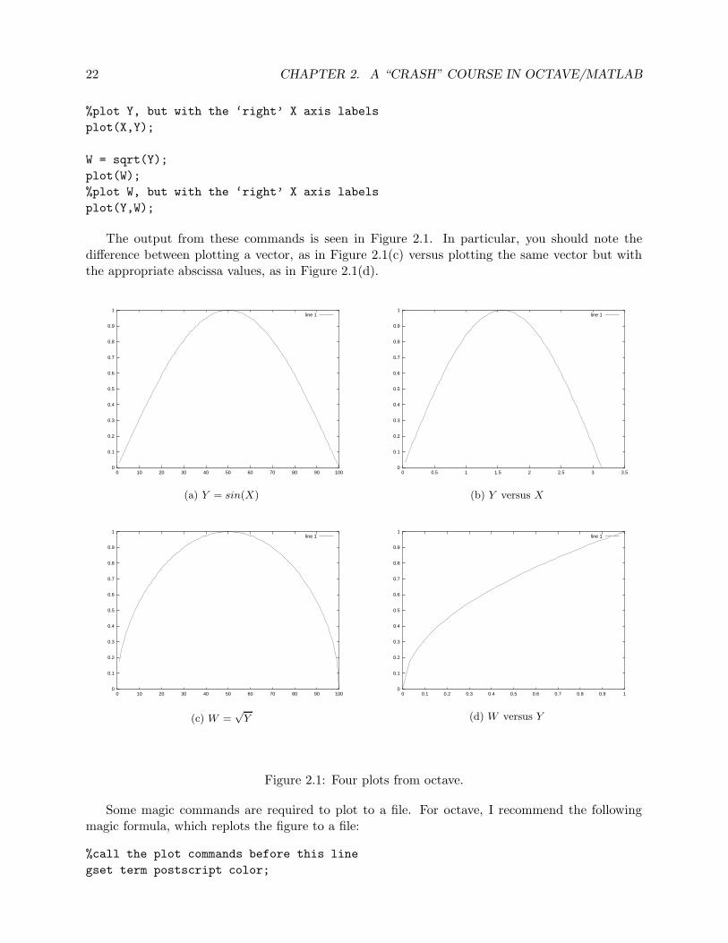
22 CHAPTER 2. A “CRASH” COURSE IN OCTAVE/MATLAB
%plot Y, but with the ‘right’ X axis labels
plot(X,Y);
W = sqrt(Y);
plot(W);
%plot W, but with the ‘right’ X axis labels
plot(Y,W);
The output from these commands is seen in Figure 2.1. In particular, you should note thedifference between plotting a vector, as in Figure 2.1(c) versus plotting the same vector but withthe appropriate abscissa values, as in Figure 2.1(d).
0
0.1
0.2
0.3
0.4
0.5
0.6
0.7
0.8
0.9
1
0 10 20 30 40 50 60 70 80 90 100
line 1
(a) Y = sin(X)
0
0.1
0.2
0.3
0.4
0.5
0.6
0.7
0.8
0.9
1
0 0.5 1 1.5 2 2.5 3 3.5
line 1
(b) Y versus X
0
0.1
0.2
0.3
0.4
0.5
0.6
0.7
0.8
0.9
1
0 10 20 30 40 50 60 70 80 90 100
line 1
(c) W =√
Y
0
0.1
0.2
0.3
0.4
0.5
0.6
0.7
0.8
0.9
1
0 0.1 0.2 0.3 0.4 0.5 0.6 0.7 0.8 0.9 1
line 1
(d) W versus Y
Figure 2.1: Four plots from octave.
Some magic commands are required to plot to a file. For octave, I recommend the followingmagic formula, which replots the figure to a file:
%call the plot commands before this line
gset term postscript color;

2.4. PLOTTING 23
gset output "filename.ps";
replot;
gset term x11;
gset output "/dev/null";
In Matlab, the commands are something like this:
%call the plot commands before this line
print(gcf,’-deps’,’filename.eps’);

24 CHAPTER 2. A “CRASH” COURSE IN OCTAVE/MATLAB
Exercises
(2.1) What do the following pieces of octave/Matlab code accomplish?(a) x = (0:40) ./ 40;
(b) a = 2;
b = 5;
x = a + (b-a) .* (0:40) ./ 40;
(c) x = a + (b-a) .* (0:40) ./ 40;
y = sin(x);
plot(x,y);
(2.2) Implement the naıve quadratic formula to find the roots of x2 + bx+ c = 0, for real b, c. Yourcode should return
−b±√b2 − 4c
2.
Your m-file should have header line like:function [x1,x2] = naivequad(b,c)
Test your code for (b, c) =(
1× 10¹⁵, 1)
. Do you get a spurious root?(2.3) Implement a robust quadratic formula (cf. Example Problem 1.9) to find the roots of x2 +
bx+ c = 0. Your m-file should have header line like:function [x1,x2] = robustquad(b,c)
Test your code for (b, c) =(
1× 10¹⁵, 1)
. Do you get a spurious root?(2.4) Write octave/Matlab code to find a fixed point for the cosine, i.e., some x such that x =
cos(x). Do this as follows: pick some initial value x0, then let xi+1 = cos(xi) for i =0, 1, . . . , n. Pick n to be reasonably large, or choose some convergence criterion (i.e., ter-minate if |xi+1 − xi| < 1× 10⁻¹⁰). Does your code always converge?
(2.5) Write code to implement the factorial function for integers:function [nfact] = factorial(n)
where n factorial is equal to 1 · 2 · 3 · · · (n− 1) ·n. Either use a ‘for’ loop, or write the functionto recursively call itself.

Chapter 3
Solving Linear Systems
A number of problems in numerical analysis can be reduced to, or approximated by, a system oflinear equations.
3.1 Gaussian Elimination with Naıve Pivoting
Our goal is the automatic solution of systems of linear equations:
a11x1 + a12x2 + a13x3 + · · · + a1nxn = b1a21x1 + a22x2 + a23x3 + · · · + a2nxn = b2a31x1 + a32x2 + a33x3 + · · · + a3nxn = b3
......
.... . .
......
an1x1 + an2x2 + an3x3 + · · · + annxn = bn
In these equations, the aij and bi are given real numbers. We also write this as
Ax = b,
where A is a matrix, whose element in the ith row and jth column is aij , and b is a column vector,whose ith entry is bi.
This gives the easier way of writing this equation:
a11 a12 a13 · · · a1n
a21 a22 a23 · · · a2n
a31 a32 a33 · · · a3n...
......
. . ....
an1 an2 an3 · · · ann
x1
x2
x3...xn
=
b1b2b3...bn
(3.1)
3.1.1 Elementary Row Operations
You may remember that one way to solve linear equations is by applying elementary row operations
to a given equation of the system. For example, if we are trying to solve the given system ofequations, they should have the same solution as the following system:
25
26 CHAPTER 3. SOLVING LINEAR SYSTEMS
a11 a12 a13 · · · a1n
a21 a22 a23 · · · a2n
a31 a32 a33 · · · a3n...
......
. . ....
κai1 κai2 κai3 · · · κain...
......
. . ....
an1 an2 an3 · · · ann
x1
x2
x3...xi...xn
=
b1b2b3...κbi...bn
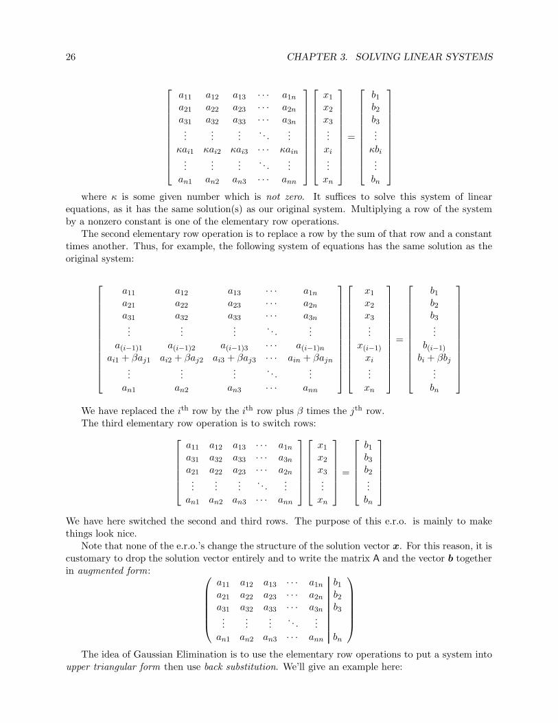
where κ is some given number which is not zero. It suffices to solve this system of linearequations, as it has the same solution(s) as our original system. Multiplying a row of the systemby a nonzero constant is one of the elementary row operations.
The second elementary row operation is to replace a row by the sum of that row and a constanttimes another. Thus, for example, the following system of equations has the same solution as theoriginal system:
a11 a12 a13 · · · a1n
a21 a22 a23 · · · a2n
a31 a32 a33 · · · a3n...
......
. . ....
a(i−1)1 a(i−1)2 a(i−1)3 · · · a(i−1)n
ai1 + βaj1 ai2 + βaj2 ai3 + βaj3 · · · ain + βajn...
......
. . ....
an1 an2 an3 · · · ann
x1
x2
x3...
x(i−1)
xi...xn
=
b1b2b3...
b(i−1)
bi + βbj...bn
We have replaced the ith row by the ith row plus β times the jth row.The third elementary row operation is to switch rows:
a11 a12 a13 · · · a1n
a31 a32 a33 · · · a3n
a21 a22 a23 · · · a2n...
......
. . ....
an1 an2 an3 · · · ann
x1
x2
x3...xn
=
b1b3b2...bn
We have here switched the second and third rows. The purpose of this e.r.o. is mainly to makethings look nice.
Note that none of the e.r.o.’s change the structure of the solution vector x. For this reason, it iscustomary to drop the solution vector entirely and to write the matrix A and the vector b togetherin augmented form:
a11 a12 a13 · · · a1n b1a21 a22 a23 · · · a2n b2a31 a32 a33 · · · a3n b3...
......
. . ....
an1 an2 an3 · · · ann bn
The idea of Gaussian Elimination is to use the elementary row operations to put a system intoupper triangular form then use back substitution. We’ll give an example here:
3.1. GAUSSIAN ELIMINATION WITH NAIVE PIVOTING 27
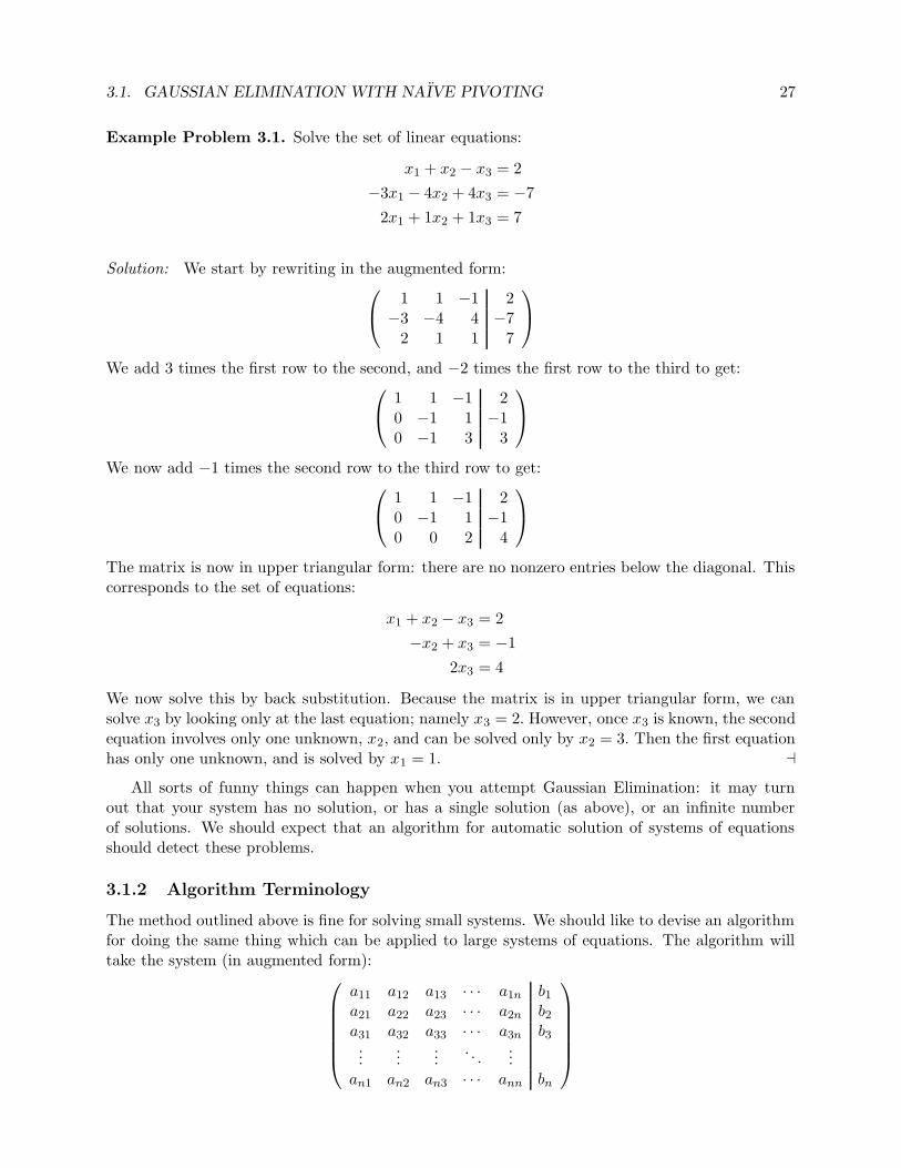
Example Problem 3.1. Solve the set of linear equations:
x1 + x2 − x3 = 2
−3x1 − 4x2 + 4x3 = −7
2x1 + 1x2 + 1x3 = 7
Solution: We start by rewriting in the augmented form:
1 1 −1 2−3 −4 4 −7
2 1 1 7
We add 3 times the first row to the second, and −2 times the first row to the third to get:
1 1 −1 20 −1 1 −10 −1 3 3
We now add −1 times the second row to the third row to get:
1 1 −1 20 −1 1 −10 0 2 4
The matrix is now in upper triangular form: there are no nonzero entries below the diagonal. Thiscorresponds to the set of equations:
x1 + x2 − x3 = 2
−x2 + x3 = −1
2x3 = 4
We now solve this by back substitution. Because the matrix is in upper triangular form, we cansolve x3 by looking only at the last equation; namely x3 = 2. However, once x3 is known, the secondequation involves only one unknown, x2, and can be solved only by x2 = 3. Then the first equationhas only one unknown, and is solved by x1 = 1. a
All sorts of funny things can happen when you attempt Gaussian Elimination: it may turnout that your system has no solution, or has a single solution (as above), or an infinite numberof solutions. We should expect that an algorithm for automatic solution of systems of equationsshould detect these problems.
3.1.2 Algorithm Terminology
The method outlined above is fine for solving small systems. We should like to devise an algorithmfor doing the same thing which can be applied to large systems of equations. The algorithm willtake the system (in augmented form):
a11 a12 a13 · · · a1n b1a21 a22 a23 · · · a2n b2a31 a32 a33 · · · a3n b3...
......
. . ....
an1 an2 an3 · · · ann bn

28 CHAPTER 3. SOLVING LINEAR SYSTEMS
The algorithm then selects the first row as the pivot equation or pivot row, and the first element ofthe first row, a11 is the pivot element. The algorithm then pivots on the pivot element to get thesystem:
a11 a12 a13 · · · a1n b10 a′22 a′23 · · · a′2n b′20 a′32 a′33 · · · a′3n b′3...
......
. . ....
0 a′n2 a′n3 · · · a′nn b′n
Wherea′ij = aij −
(
ai1a11
)
a1j
b′i = bi −(
ai1a11
)
b1
(2 ≤ i ≤ n, 1 ≤ j ≤ n)
Effectively we are carrying out the e.r.o. of replacing the ith row by the ith row minus(
ai1a11
)
times
the first row. The quantity(
ai1a11
)
is the multiplier for the ith row.
Hereafter the algorithm will not alter the first row or first column of the system. Thus, thealgorithm could be written recursively. By pivoting on the second row, the algorithm then generatesthe system:
a11 a12 a13 · · · a1n b10 a′22 a′23 · · · a′2n b′20 0 a′′33 · · · a′′3n b′′3...
......
. . ....
0 0 a′′n3 · · · a′′nn b′′n
In this casea′′ij = a′ij −
(
a′
i2a′
22
)
a′2j
b′′i = b′i −(
a′
i2a′
22
)
b′2
(3 ≤ i ≤ n, 1 ≤ j ≤ n)
3.1.3 Algorithm Problems
The pivoting strategy we examined in this section is called ‘naıve’ because a real algorithm is a bitmore complicated. The algorithm we have outlined is far too rigid–it always chooses to pivot onthe kth row during the kth step. This would be bad if the pivot element were zero; in this case allthe multipliers aik
akkare not defined.
Bad things can happen if akk is merely small instead of zero. Consider the following example:
Example 3.2. Solve the system of equations given by the augmented form:
(
−0.0590 0.2372 −0.35280.1080 −0.4348 0.6452
)
Note that the exact solution of this system is x1 = 10, x2 = 1. Suppose, however, that the algorithmuses only 4 significant figures for its calculations. The algorithm, naıvely, pivots on the firstequation. The multiplier for the second row is
0.1080
−0.0590≈ −1.830508...,
which will be rounded to −1.831 by the algorithm.

3.2. PIVOTING STRATEGIES FOR GAUSSIAN ELIMINATION 29
The second entry in the matrix is replaced by
−0.4348 − (−1.831)(0.2372) = −0.4348 + 0.4343 = −0.0005,
where the arithmetic is rounded to four significant figures each time. There is some serious sub-tractive cancellation going on here. We have lost three figures with this subtraction. The errorsget worse from here. Similarly, the second vector entry becomes:
0.6452 − (−1.831)(−0.3528) = 0.6452 − 0.6460 = −0.0008,
where, again, intermediate steps are rounded to four significant figures, and again there is subtrac-tive cancelling. This puts the system in the form
(
−0.0590 0.2372 −0.35280 −0.0005 −0.0008
)
When the algorithm attempts back substitution, it gets the value
x2 =−0.0008
−0.0005= 1.6.
This is a bit off from the actual value of 1. The algorithm now finds
x1 = (−0.3528 − 0.2372 · 1.6) /−0.059 = (−0.3528 − 0.3795) /−0.059 = (−0.7323) /−0.059 = 12.41,
where each step has rounding to four significant figures. This is also a bit off.
3.2 Pivoting Strategies for Gaussian Elimination
Gaussian Elimination can fail when performed in the wrong order. If the algorithm selects a zeropivot, the multipliers are undefined, which is no good. We also saw that a pivot small in magnitudecan cause failure. As here:
εx1 + x2 = 1
x1 + x2 = 2
The naıve algorithm solves this as
x2 =2− 1
ε
1− 1ε
= 1− ε
1− ε
x1 =1− x2
ε=
1
1− ε
If ε is very small, then 1ε is enormous compared to both 1 and 2. With poor rounding, the algorithm
solves x2 as 1. Then it solves x1 = 0. This is nearly correct for x2, but is an awful approximationfor x1. Note that this choice of x1, x2 satisfies the first equation, but not the second.
Now suppose the algorithm changed the order of the equations, then solved:
x1 + x2 = 2
εx1 + x2 = 1

30 CHAPTER 3. SOLVING LINEAR SYSTEMS
The algorithm solves this as
x2 =1− 2ε
1− εx1 = 2− x2
There’s no problem with rounding here.The problem is not the small entry per se: Suppose we use an e.r.o. to scale the first equation,
then use naıve G.E.:
x1 +1
εx2 =
1
εx1 + x2 = 2
This is still solved as
x2 =2− 1
ε
1− 1ε
x1 =1− x2
ε,
and rounding is still a problem.
3.2.1 Scaled Partial Pivoting
The naıve G.E. algorithm uses the rows 1, 2, . . . , n-1 in order as pivot equations. As shown above,this can cause errors. Better is to pivot first on row `1, then row `2, etc, until finally pivoting onrow `n−1, for some permutation {`i}ni=1 of the integers 1, 2, . . . , n. The strategy of scaled partial
pivoting is to compute this permutation so that G.E. works well.In light of our example, we want to pivot on an element which is not small compared to other
elements in its row. So our algorithm first determines “smallness” by calculating a scale, row-wise:
si = max1≤j≤n
|aij | .
The scales are only computed once.Then the first pivot, `1, is chosen to be the i such that
|ai,1|si
is maximized. The algorithm pivots on row `1, producing a bunch of zeros in the first column. Notethat the algorithm should not rearrange the matrix–this takes too much work.
The second pivot, `2, is chosen to be the i such that
|ai,2|si
is maximized, but without choosing `2 = `1. The algorithm pivots on row `2, producing a bunch ofzeros in the second column.
In the kth step `k is chosen to be the i not among `1, `2, . . . , `k−1 such that
|ai,k|si
3.2. PIVOTING STRATEGIES FOR GAUSSIAN ELIMINATION 31
is maximized. The algorithm pivots on row `k, producing a bunch of zeros in the kth column.The slick way to implement this is to first set `i = i for i = 1, 2, . . . , n. Then rearrange this
vector in a kind of “bubble sort”: when you find the index that should be `1, swap them, i.e., findthe j such that `j should be the first pivot and switch the values of `1, `j.
Then at the kth step, search only those indices in the tail of this vector: i.e., only among `j fork ≤ j ≤ n, and perform a swap.
3.2.2 An Example
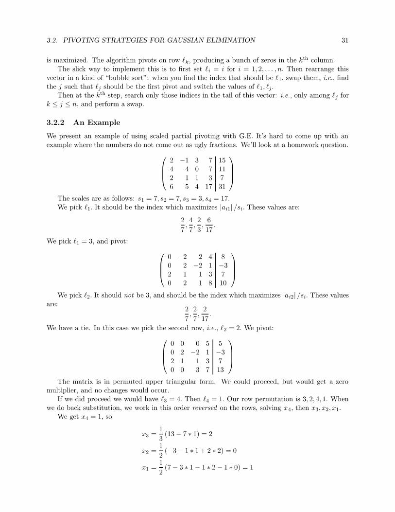
We present an example of using scaled partial pivoting with G.E. It’s hard to come up with anexample where the numbers do not come out as ugly fractions. We’ll look at a homework question.
2 −1 3 7 154 4 0 7 112 1 1 3 76 5 4 17 31
The scales are as follows: s1 = 7, s2 = 7, s3 = 3, s4 = 17.We pick `1. It should be the index which maximizes |ai1| /si. These values are:
2
7,4
7,2
3,
6
17.
We pick `1 = 3, and pivot:
0 −2 2 4 80 2 −2 1 −32 1 1 3 70 2 1 8 10
We pick `2. It should not be 3, and should be the index which maximizes |ai2| /si. These valuesare:
2
7,2
7,
2
17.
We have a tie. In this case we pick the second row, i.e., `2 = 2. We pivot:
0 0 0 5 50 2 −2 1 −32 1 1 3 70 0 3 7 13
The matrix is in permuted upper triangular form. We could proceed, but would get a zeromultiplier, and no changes would occur.
If we did proceed we would have `3 = 4. Then `4 = 1. Our row permutation is 3, 2, 4, 1. Whenwe do back substitution, we work in this order reversed on the rows, solving x4, then x3, x2, x1.
We get x4 = 1, so
x3 =1
3(13− 7 ∗ 1) = 2
x2 =1
2(−3− 1 ∗ 1 + 2 ∗ 2) = 0
x1 =1
2(7− 3 ∗ 1− 1 ∗ 2− 1 ∗ 0) = 1
32 CHAPTER 3. SOLVING LINEAR SYSTEMS
3.2.3 Another Example and A Real Algorithm
Sometimes we want to solve
Ax = b
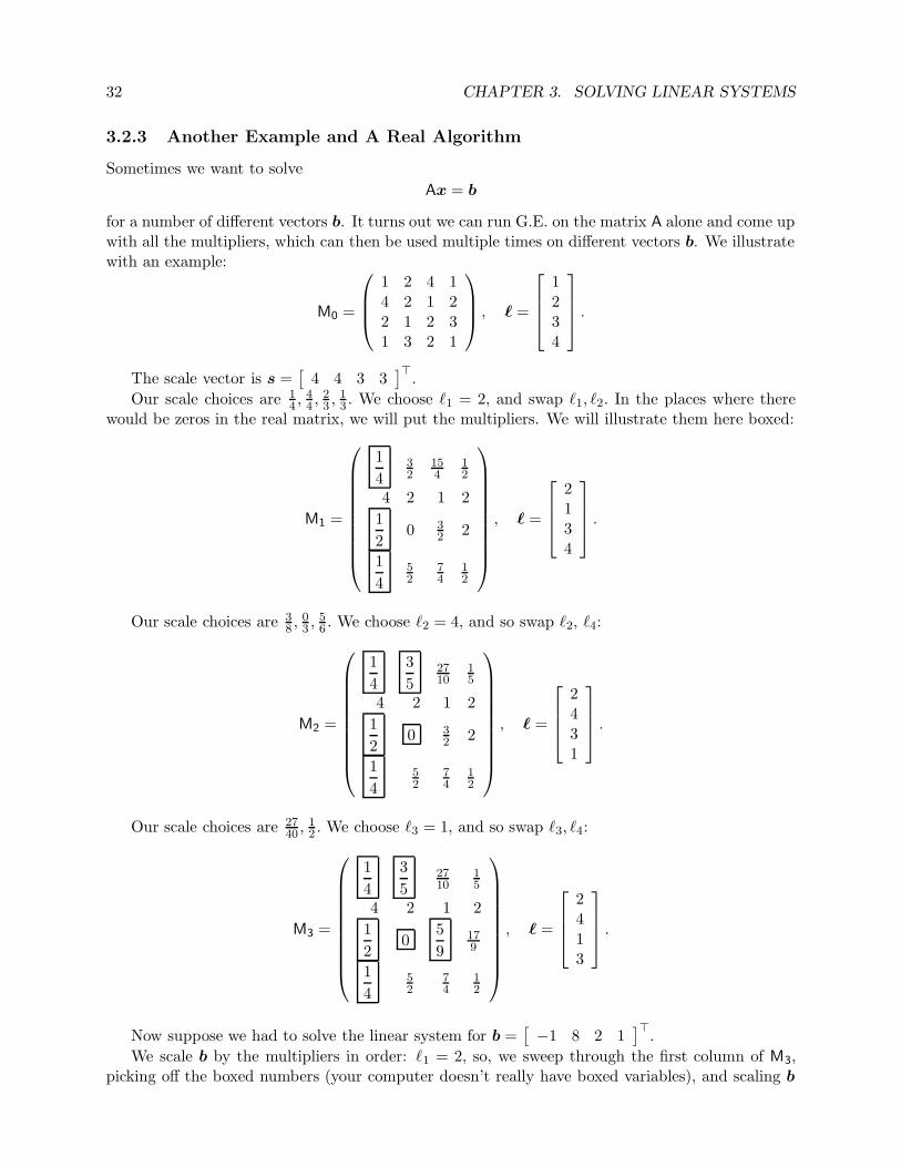
for a number of different vectors b. It turns out we can run G.E. on the matrix A alone and come upwith all the multipliers, which can then be used multiple times on different vectors b. We illustratewith an example:
M0 =
1 2 4 14 2 1 22 1 2 31 3 2 1
, ` =
1234
.
The scale vector is s =[
4 4 3 3]>
.
Our scale choices are 14 ,
44 ,
23 ,
13 . We choose `1 = 2, and swap `1, `2. In the places where there
would be zeros in the real matrix, we will put the multipliers. We will illustrate them here boxed:
M1 =
1
432
154
12
4 2 1 2
1
20 3
2 2
1
452
74
12
, ` =
2134
.
Our scale choices are 38 ,
03 ,
56 . We choose `2 = 4, and so swap `2, `4:
M2 =
1
4
3
52710
15
4 2 1 2
1
20 3
2 2
1
452
74
12
, ` =
2431
.
Our scale choices are 2740 ,
12 . We choose `3 = 1, and so swap `3, `4:
M3 =
1
4
3
52710
15
4 2 1 2
1
20
5
9179
1
452
74
12
, ` =
2413
.
Now suppose we had to solve the linear system for b =[
−1 8 2 1]>
.
We scale b by the multipliers in order: `1 = 2, so, we sweep through the first column of M3,picking off the boxed numbers (your computer doesn’t really have boxed variables), and scaling b

3.3. LU FACTORIZATION 33
appropriately:
−1821
⇒
−38−2−1
This continues:
−38−2−1
⇒
−125
8−2−1
⇒
−125
8−2
3−1
We then perform a permuted backwards substitution on the augmented system
0 0 2710
15 −12
54 2 1 2 80 0 0 17
9 −23
0 52
74
12 −1
This proceeds as
x4 =−2
3
9
17=−6
17
x3 =10
27
(
−12
5− 1
5
−6
17
)
= . . .
x2 =2
5
(
−1− 1
2
−6
17− 7
4x3
)
= . . .
x1 =1
4
(
8− 2−6
17− x3 − 2x2
)
= . . .
Fill in your own values here.
3.3 LU Factorization
We examined G.E. to solve the systemAx = b,
where A is a matrix:
A =
a11 a12 a13 · · · a1n
a21 a22 a23 · · · a2n
a31 a32 a33 · · · a3n...
......
. . ....
an1 an2 an3 · · · ann
.
We want to show that G.E. actually factors A into lower and upper triangular parts, that is A = LU,where
L =
1 0 0 · · · 0`21 1 0 · · · 0`31 `32 1 · · · 0...
......
. . ....
`n1 `n2 `n3 · · · 1
, U =
u11 u12 u13 · · · u1n
0 u22 u23 · · · u2n
0 0 u33 · · · u3n...
......
. . ....
0 0 0 · · · unn
.
We call this a LU Factorization of A.

34 CHAPTER 3. SOLVING LINEAR SYSTEMS
3.3.1 An Example
We consider solution of the following augmented form:
2 1 1 3 74 4 0 7 116 5 4 17 312 −1 0 7 15
(3.2)
The naıve G.E. reduces this to
2 1 1 3 70 2 −2 1 −30 0 3 7 130 0 0 12 18
We are going to run the naıve G.E., and see how it is a LU Factorization. Since this is the naıveversion, we first pivot on the first row. Our multipliers are 2, 3, 1. We pivot to get
2 1 1 3 70 2 −2 1 −30 2 1 8 100 −2 −1 4 8
Careful inspection shows that we’ve merely multiplied A and b by a lower triangular matrix M1:
M1 =
1 0 0 0−2 1 0 0−3 0 1 0−1 0 0 1
The entries in the first column are the negative e.r.o. multipliers for each row. Thus after the firstpivot, it is like we are solving the system
M1Ax = M1b.
We pivot on the second row to get:
2 1 1 3 70 2 −2 1 −30 0 3 7 130 0 −3 5 5
The multipliers are 1,−1. We can view this pivot as a multiplication by M2, with
M2 =
1 0 0 00 1 0 00 −1 1 00 1 0 1
We are now solving
M2M1Ax = M2M1b.
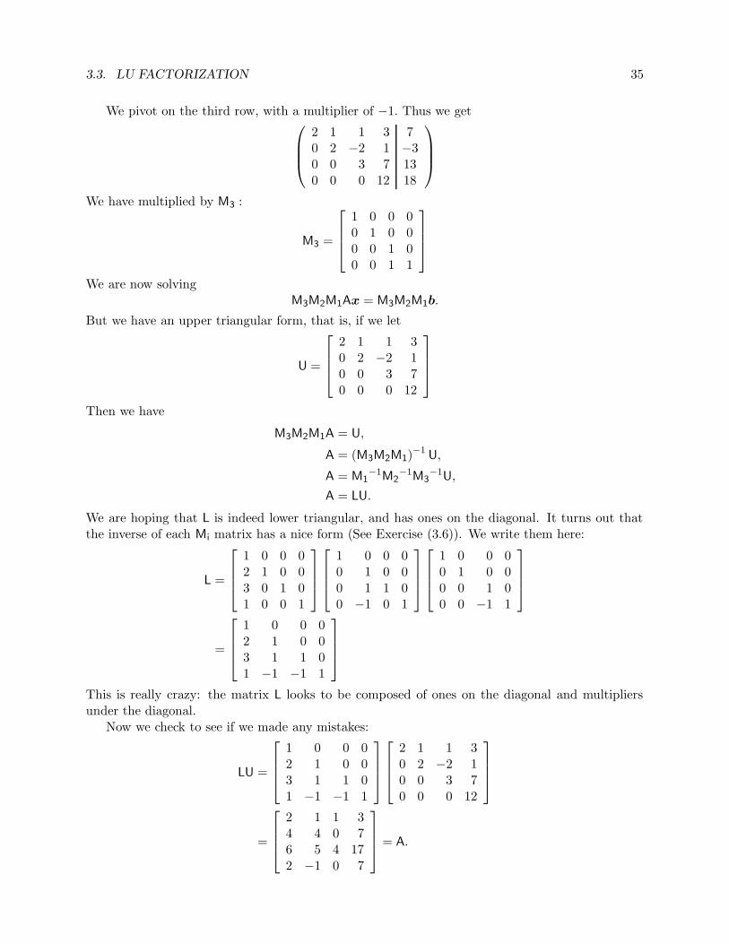
3.3. LU FACTORIZATION 35
We pivot on the third row, with a multiplier of −1. Thus we get
2 1 1 3 70 2 −2 1 −30 0 3 7 130 0 0 12 18
We have multiplied by M3 :
M3 =
1 0 0 00 1 0 00 0 1 00 0 1 1
We are now solvingM3M2M1Ax = M3M2M1b.
But we have an upper triangular form, that is, if we let
U =
2 1 1 30 2 −2 10 0 3 70 0 0 12
Then we have
M3M2M1A = U,
A = (M3M2M1)−1
U,
A = M1−1M2
−1M3−1U,
A = LU.
We are hoping that L is indeed lower triangular, and has ones on the diagonal. It turns out thatthe inverse of each Mi matrix has a nice form (See Exercise (3.6)). We write them here:
L =
1 0 0 02 1 0 03 0 1 01 0 0 1
1 0 0 00 1 0 00 1 1 00 −1 0 1
1 0 0 00 1 0 00 0 1 00 0 −1 1
=
1 0 0 02 1 0 03 1 1 01 −1 −1 1
This is really crazy: the matrix L looks to be composed of ones on the diagonal and multipliersunder the diagonal.
Now we check to see if we made any mistakes:
LU =
1 0 0 02 1 0 03 1 1 01 −1 −1 1
2 1 1 30 2 −2 10 0 3 70 0 0 12
=
2 1 1 34 4 0 76 5 4 172 −1 0 7
= A.

36 CHAPTER 3. SOLVING LINEAR SYSTEMS
3.3.2 Using LU Factorizations
We see that the G.E. algorithm can be used to actually calculate the LU factorization. We will lookat this in more detail in another example. We now examine how we can use the LU factorizationto solve the equation
Ax = b,
Since we have A = LU, we first solve
Lz = b,
then solve
Ux = z.
Since L is lower triangular, we can solve for z with a forward substitution. Similarly, since U isupper triangular, we can solve for x with a back substitution. We drag out the previous example(which we never got around to solving):
2 1 1 3 74 4 0 7 116 5 4 17 312 −1 0 7 15
We had found the LU factorization of A as
A =
1 0 0 02 1 0 03 1 1 01 −1 −1 1
2 1 1 30 2 −2 10 0 3 70 0 0 12
So we solve
1 0 0 02 1 0 03 1 1 01 −1 −1 1
z =
7113115
We get
z =
7−31318
Now we solve
2 1 1 30 2 −2 10 0 3 70 0 0 12
x =
7−31318
We get the ugly solution
z =
3724−17125632

3.4. ITERATIVE SOLUTIONS 37
3.3.3 Some Theory
We aren’t doing much proving here. The following theorem has an ugly proof in the Cheney &Kincaid [7].
Theorem 3.3. If A is an n×n matrix, and naıve Gaussian Elimination does not encounter a zeropivot, then the algorithm generates a LU factorization of A, where L is the lower triangular part ofthe output matrix, and U is the upper triangular part.
This theorem relies on us using the fancy version of G.E., which saves the multipliers in thespots where there should be zeros. If correctly implemented, then, L is the lower triangular partbut with ones put on the diagonal.
This theorem is proved in Cheney & Kincaid [7]. This appears to me to be a case of somethingwhich can be better illustrated with an example or two and some informal investigation. The proofis an unillustrating index-chase–read it at your own risk.
3.3.4 Computing Inverses
We consider finding the inverse of A. Since
AA−1 = I,
then the jth column of the inverse A−1 solves the equation
Ax = ej ,
where ej is the column matrix of all zeros, but with a one in the j th position.Thus we can find the inverse of A by running n linear solves. Obviously we are only going
to run G.E. once, to put the matrix in LU form, then run n solves using forward and backwardsubstitutions.
3.4 Iterative Solutions
Recall we are trying to solveAx = b.
We examine the computational cost of Gaussian Elimination to motivate the search for an alter-native algorithm.
3.4.1 An Operation Count for Gaussian Elimination
We consider the number of floating point operations (“flops”) required to solve the system Ax = b.Gaussian Elimnation first uses row operations to transform the problem into an equivalent problemof the form Ux = b′, where U is upper triangular. Then back substitution is used to solve for x.
First we look at how many floating point operations are required to reduce
a11 a12 a13 · · · a1n b1a21 a22 a23 · · · a2n b2a31 a32 a33 · · · a3n b3...
......
. . ....
an1 an2 an3 · · · ann bn

38 CHAPTER 3. SOLVING LINEAR SYSTEMS
to
a11 a12 a13 · · · a1n b10 a′22 a′23 · · · a′2n b′20 a′32 a′33 · · · a′3n b′3...
......
. . ....
0 a′n2 a′n3 · · · a′nn b′n
First a multiplier is computed for each row. Then in each row the algorithm performs nmultiplies and n adds. This gives a total of (n−1)+(n−1)n multiplies (counting in the computingof the multiplier in each of the (n− 1) rows) and (n− 1)n adds. In total this is 2n2−n− 1 floatingpoint operations to do a single pivot on the n by n system.
Then this has to be done recursively on the lower right subsystem, which is an (n−1) by (n−1)system. This requires 2(n − 1)2 − (n − 1) − 1 operations. Then this has to be done on the nextsubsystem, requiring 2(n− 2)2 − (n− 2)− 1 operations, and so on.
In total, then, we use In total floating point operations, with
In = 2
n∑
j=1
j2 −n∑
j=1
j −n∑
j=1
1.
Recalling that
n∑
j=1
j2 =1
6(n)(n+ 1)(2n+ 1), and
n∑
j=1
j =1
2(n)(n+ 1),
We find that
In =1
6(4n− 1)n(n+ 1)− n ≈ 2
3n3.
Now consider the costs of back substitution. To solve
a11 · · · a1,n−2 a1,n−1 a1n b1...
. . ....
......
...0 · · · an−2,n−2 an−2,n−1 an−2,n bn−2
0 · · · 0 an−1,n−1 an−1,n bn−1
0 · · · 0 0 ann bn
for xn requires only a single division. Then to solve for xn−1 we compute
xn−1 =1
an−1,n−1[bn−1 − an−1,nxn] ,
and requires 3 flops. Similarly, solving for xn−2 requires 5 flops. Thus in total back substitutionrequires Bn total floating point operations with
Bn =
n∑
j=1
2j − 1 = n(n− 1)− n = n(n− 2) ≈ n2

3.4. ITERATIVE SOLUTIONS 39
3.4.2 Dividing by Multiplying
We saw that Gaussian Elimination requires around 23n
3 operations just to find the LU factorization,then about n2 operations to solve the system, when A is n×n. When n is large, this may take toolong to be practical. Additionally, if A is sparse (has few nonzero elements per row), we would likethe complexity of our computations to scale with the sparsity of A. Thus we look for an alternativealgorithm.
First we consider the simplest case, n = 1. Suppose we are to solve the equation
Ax = b.
for scalars A, b. We solve this by
x =1
Ab =
1
ωAωb =
1
1− (1− ωA)ωb =
1
1− rωb,
where ω 6= 0 is some real number chosen to “weight” the problem appropriately, and r = 1 − ωA.Now suppose that ω is chosen such that |r| < 1. This can be done so long as A 6= 0, which wouldhave been a problem anyway. Now use the geometric expansion:
1
1− r = 1 + r + r2 + r3 + . . .
Because of the assumption |r| < 1, the terms rn converge to zero as n → ∞. This gives theapproximate solution to our one dimensional problem as
x ≈[
1 + r + r2 + r3 + . . .+ rk]
ωb
= ωb+[
r + r2 + r3 + . . .+ rk]
ωb
= ωb+ r[
1 + r + r2 + . . .+ rk−1]
ωb
This suggests an iterative approach to solving Ax = b. First let x(0) = ωb, then let
x(k) = ωb+ rx(k−1).
The iterates x(k) will converge to the solution of Ax = b if |r| < 1.You should now convince yourself that because rn → 0, that the choice of the initial iterate x(0)
was immaterial, i.e., that under any choice of initial iterate convergence is guaranteed.We now translate this scalar result into the vector case. The algorithm proceeds as follows: first
fix some initial estimate of the solution, x(0). A good choice might be ωb, but this is not necessary.Then calculate successive approximations to the actual solution by updates of the form
x(k) = ωb + (I− ωA)x(k−1).
It turns out that we can consider a slightly more general form of the algorithm, one in whichsuccessive iterates are defined implicitly. That is we consider iterates of the form
Qx(k+1) = (Q− ωA)x(k) + ωb, (3.3)
for some matrix Q, and some scaling factor ω. Note that this update relies on vector additionsand possibly by premultiplication of a vector by A or Q. In the case where these two matrices aresparse, such an update can be relatively cheap.

40 CHAPTER 3. SOLVING LINEAR SYSTEMS
Now suppose that as k → ∞, x(k) converges to some vector x∗, which is a fixed point of theiteration. Then
Qx∗ = (Q− ωA)x∗ + ωb,
Qx∗ = Qx∗ − ωAx∗ + ωb,
ωAx∗ = ωb,
Ax∗ = b.
We have some freedom in choosing Q, but there are two considerations we should keep in mind:1. Choice of Q affects convergence and speed of convergence of the method. In particular, we
want Q to be similar to A.2. Choice of Q affects ease of computing the update. That is, given
z = (Q− A)x(k) + b,
we should pick Q such that the equation
Qx(k+1) = z
is easy to solve exactly.These two goals conflict with each other. At one end of the spectrum is the so-called “impossibleiteration,” at the other is the Richardsons.
3.4.3 Impossible Iteration
I made up the term “impossible iteration.” But consider the method which takes Q to be A. Thisseems to be the best choice for satisfying the first goal. Letting ω = 1, our method becomes
Ax(k+1) = (A− A)x(k) + b = b.
This method should clearly converge in one step. However, the second goal is totally ignored.Indeed, we are considering iterative methods because we cannot easily solve this linear equation inthe first place.
3.4.4 Richardson Iteration
At the other end of the spectrum is the Richardson Iteration, which chooses Q to be the identitymatrix. Solving the system
Qx(k+1) = z
is trivial: we just have x(k+1) = z.
Example Problem 3.4. Use Richardson Iteration with ω = 1 on the system
A =
6 1 12 4 01 2 6
, b =
1206
.
Solution: We let
Q =
1 0 00 1 00 0 1
, (Q− A) =
−5 −1 −1−2 −3 0−1 −2 −5
.

3.4. ITERATIVE SOLUTIONS 41
We start with an arbitrary x(0), say x(0) = [2 2 2]> . We get x(1) = [−2 − 10 − 10]> , and x(2) =[42 34 78]> .
Note the real solution is x = [2 − 1 1]> . The Richardson Iteration does not appear to convergefor this example, unfortunately. a
Example Problem 3.5. Apply Richardson Iteration with ω = 1/6 on the previous system.Solution: Our iteration becomes
x(k+1) =
0 −1/6 −1/6−1/3 1/3 0−1/6 −1/3 0
x(k) +
201
.
We start with the same x(0) as previously, x(0) = [2 2 2]> . We get x(1) = [4/3 0 0]> , x(2) =[2 − 4/9 7/9]> , and finally x(12) = [2 − 0.99998 0.99998]> .
Thus, the choice of ω has some affect on convergence. a
We can rethink the Richardson Iteration as
x(k+1) = (I− ωA)x(k) + ωb = x(k) + ω(
b− Ax(k))
.
Thus at each step we are adding some scaled version of the residual, defined as b − Ax(k), to theiterate.
3.4.5 Jacobi Iteration
The Jacobi Iteration chooses Q to be the matrix consisting of the diagonal of A. This is moresimilar to A than the identity matrix, but nearly as simple to invert.
Example Problem 3.6. Use Jacobi Iteration, with ω = 1, to solve the system
A =
6 1 12 4 01 2 6
, b =
1206
.
Solution: We let
Q =
6 0 00 4 00 0 6
, (Q− A) =
0 −1 −1−2 0 0−1 −2 0
, Q−1 =
16 0 00 1
4 00 0 1
6
.
We start with an arbitrary x(0), say x(0) = [2 2 2]> . We get x(1) =[
43 − 1 0
]>. Then x(2) =
[
136 − 2
3109
]>. Continuing, we find that x(5) ≈ [1.987 − 1.019 0.981]> .
Note the real solution is x = [2 − 1 1]> . a
There is an alternative way to describe the Jacobi Iteration for ω = 1. By considering the updateelementwise, we see that the operation can be described by
x(k+1)j =
1
ajj
bj −n∑
i=1,i6=j
ajix(k)i
.
Thus an update takes less than 2n2 operations. In fact, if A is sparse, with less than k nonzeroentries per row, the update should take less than 2nk operations.

42 CHAPTER 3. SOLVING LINEAR SYSTEMS
3.4.6 Gauss Seidel Iteration
The Gauss Seidel Iteration chooses Q to be lower triangular part of A, including the diagonal. Inthis case solving the system
Qx(k+1) = z
is performed by forward substitution. Here the Q is more like A than for Jacobi Iteration, butinvolves more work for inverting.
Example Problem 3.7. Use Gauss Seidel Iteration to again solve for
A =
6 1 12 4 01 2 6
, b =
1206
.
Solution: We let
Q =
6 0 02 4 01 2 6
, (Q− A) =
0 −1 −10 0 00 0 0
.
We start with an arbitrary x(0), say x(0) = [2 2 2]> . We get x(1) =[
43 − 2
3 1]>. Then x(2) =
[
3518 − 35
36 1]>.
Already this is fairly close to the actual solution x = [2 − 1 1]> . a
Just as with Jacobi Iteration, there is an easier way to describe the Gauss Seidel Iteration. Inthis case we will keep a single vector x and overwrite it, element by element. Thus for j = 1, 2, . . . , n,we set
xj ←1
ajj
bj −n∑
i=1,i6=j
ajixi
.
This looks exactly like the Jacobi update. However, in the sum on the right there are some “old”values of xi and some “new” values; the new values are those xi for which i < j.
Again this takes less than 2n2 operations. Or less than 2nk if A is sufficiently sparse.
An alteration of the Gauss Seidel Iteration is to make successive “sweeps” of this redefinition,one for j = 1, 2, . . . , n, the next for j = n, n − 1, . . . , 2, 1. This amounts to running Gauss Seidelonce with Q the lower triangular part of A, then running it with Q the upper triangular part. Thisiterative method is known as “red-black Gauss Seidel.”
3.4.7 Error Analysis
Suppose that x is the solution to equation 3.4. Define the error vector:
e(k) = x(k) − x.

3.4. ITERATIVE SOLUTIONS 43
Now notice that
x(k+1) = Q−1 (Q− ωA)x(k) + Q−1ωb,
x(k+1) = Q−1Qx(k) − ωQ−1Ax(k) + ωQ−1Ax,
x(k+1) = x(k) − ωQ−1A
(
x(k) − x)
,
x(k+1) − x = x(k) − x− ωQ−1A
(
x(k) − x)
,
e(k+1) = e(k) − ωQ−1Ae(k),
e(k+1) =(
I− ωQ−1A)
e(k).
Reusing this relation we find that
e(k) =(
I− ωQ−1A)
e(k−1),
=(
I− ωQ−1A)2
e(k−2),
=(
I− ωQ−1A)k
e(0).
We want to ensure that e(k+1) is “smaller” than e(k). To do this we recall matrix and vector normsfrom Subsection 1.4.1.
∥
∥
∥e(k)
∥
∥
∥
2=∥
∥
∥
(
I− ωQ−1A)k
e(0)∥
∥
∥
2≤∥
∥I− ωQ−1A∥
∥
k
2
∥
∥
∥e(0)
∥
∥
∥
2.
(See Example Problem 1.29.)
Thus our iteration converges (e(k) goes to the zero vector, i.e., x(k) → x) if
∥
∥I− ωQ−1A∥
∥
2< 1.
This gives the theorem:
Theorem 3.8. An iterative solution scheme converges for any starting x(0) if and only if alleigenvalues of I− ωQ−1A are less than 1 in absolute value, i.e., if and only if
∥
∥I− ωQ−1A∥
∥
2< 1
Another way of saying this is “the spectral radius of I− ωQ−1A is less than 1.”
In fact, the speed of convergence is decided by the spectral radius of the matrix–convergenceis faster for smaller values. Recall our introduction to iterative methods in the scalar case, wherethe result relied on ω being chosen such that |1− ωA| < 1. You should now think about howeigenvalues generalize the absolute value of a scalar, and how this relates to the norm of matrices.
Let y be an eigenvector for Q−1A, with corresponding eigenvalue λ. Then
(
I− ωQ−1A)
y = y − ωQ−1Ay = y − ωλy = (1− ωλ) y.
This relation may allow us to pick the optimal ω for given A,Q. It can also show us thatsometimes no choice of ω will give convergence of the method. There are a number of differentrelated results that show when various methods will work for certain choices of ω. We leave theseto the exercises.

44 CHAPTER 3. SOLVING LINEAR SYSTEMS
Example Problem 3.9. Find conditions on ω which guarantee convergence of Richardson’s Iter-ation for finding approximate iterative solutions to the system Ax = b, where
A =
6 1 12 4 01 2 6
, b =
1206
.
Solution: By Theorem 3.8, with Q the identity matrix, we have convergence if and only if
‖I− ωA‖2 < 1
We now use the fact that “eigenvalues commute with polynomials;” that is if f(x) is a polynomialand λ is an eigenvalue of a matrix A, then f(λ) is an eigenvalue of the matrix f(A). In this case thepolynomial we consider is f(x) = x0−ωx1. Using octave or Matlab you will find that the eigenvaluesof A are approximately 7.7321, 4.2679, and 4. Thus the eigenvalues of I− ωA are approximately
1− 7.7321ω, 1− 4.2679ω, 1− 4ω.
With some work it can be shown that all three of these values will be less than one in absolutevalue if and only if
0 < ω <3
7.7321≈ 0.388
(See also Exercise (3.10).)
Compare this to the results of Example Problem 3.4, where for this system, ω = 1 apparently didnot lead to convergence, while for Example Problem 3.5, with ω = 1/6, convergence was observed.
a
3.4.8 A Free Lunch?
The analysis leading to Theorem 3.8 leads to an interesting possible variant of the iterative scheme.For simplicity we will only consider an alteration of Richardson’s Iteration. In the altered algorithmwe presuppose the existence, via some oracle, of a sequence of weightings, ωi, which we use in eachiterative update. Thus our algorithm becomes:
1. Select some initial iterate x(0).2. Given iterate x(k−1), define
x(k) = (I− ωkA)x(k−1) + ωkb.
Following the analysis for Theorem 3.8, it can be shown that
e(k) = (I− ωkA) e(k−1)
where, again, e(k) = x(k) − x, with x the actual solution to the linear system. Expanding e(k−1)
similarly gives
e(k) = (I− ωkA) (Iωk−1A) e(k−2)
=
(
k∏
i=1
I− ωiA
)
e(0).

3.4. ITERATIVE SOLUTIONS 45
Remember that we want e(k) to be small in magnitude, or, better yet, to be zero. One way toguarantee that e(k) is zero, regardless of the choice of e(0) it to somehow ensure that the matrix
B =
k∏
i=1
I− ωiA
has all zero eigenvalues.We again make use of the fact that eigenvalues “commute” with polynomials to claim that if
λj is an eigenvalue of A, thenk∏
i=1
1− ωiλj
is an eigenvalue of B. This eigenvalue is zero if one of the ωi for 1 ≤ i ≤ k is 1/λj . This suggestshow we are to pick the weightings: let them be the inverses of the eigenvalues of A.
In fact, if A has a small number of distinct eigenvalues, say m eigenvalues, then convergence tothe exact solution could be guaranteed after only m iterations, regardless of the size of the matrix.
As you may have guessed from the title of this subsection, this is not exactly a practicalalgorithm. The problem is that it is not simple to find, for a given arbitrary matrix A, one, some,or all its eigenvalues. This problem is of sufficient complexity to outweigh any savings to be gottenfrom our “free lunch” algorithm.
However, in some limited situations this algorithm might be practical if the eigenvalues of A
are known a priori .

46 CHAPTER 3. SOLVING LINEAR SYSTEMS
Exercises
(3.1) Find the LU decomposition of the following matrices, using naıve Gaussian Elimination
(a)
3 −1 −29 −1 −4−6 10 13
(b)
8 24 161 12 114 13 19
(c)
−3 6 01 −2 0−4 5 −8
(3.2) Perform back substitution to solve the equation
1 3 5 30 2 4 30 0 2 10 0 0 2
x =
−1−112
(3.3) Perform Naıve Gaussian Elimination to prove Cramer’s rule for the 2D case. That is, provethat the solution to
[
a bc d
] [
xy
]
=
[
fg
]
is given by
y =
det
[
a fc g
]
det
[
a bc d
] and x =
det
[
f bg d
]
det
[
a bc d
]
(3.4) Implement Cramer’s rule to solve a pair of linear equations in 2 variables. Your m-file shouldhave header line like:function x = cramer2(A,b)
where A is a 2 × 2 matrix, and b and x are 2 × 1 vectors. Your code should find the x suchthat Ax = b. (See Exercise (3.3))Test your code on the following (augmented) systems:
(a)
(
3 −2 14 −3 −1
)
(b)
(
1.24 −3.48 1−0.744 2.088 2
)
(c)
(
1.24 −3.48 1−0.744 2.088 −0.6
)
(d)
(
−0.0590 0.2372 −0.35280.1080 −0.4348 0.6452
)
(3.5) Given two lines parametrized by f(t) = at+b, and g(s) = cs+d, set up a linear 2×2 systemof equations to find the t, s at the point of intersection of the two lines. If you were goingto write a program to detect the intersection of two lines, how would you detect whetherthey are parallel? How is this related to the form of the solution to a system of two linearequations? (See Exercise (3.3))
(3.6) Prove that the inverse of the matrix
1 0 0 · · · 0a2 1 0 · · · 0a3 0 1 · · · 0...
......
. . ....
an 0 0 · · · 1
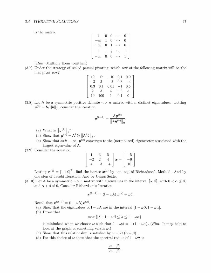
3.4. ITERATIVE SOLUTIONS 47
is the matrix
1 0 0 · · · 0−a2 1 0 · · · 0−a3 0 1 · · · 0
......
.... . .
...−an 0 0 · · · 1
(Hint: Multiply them together.)(3.7) Under the strategy of scaled partial pivoting, which row of the following matrix will be the
first pivot row?
10 17 −10 0.1 0.9−3 3 −3 0.3 −40.3 0.1 0.01 −1 0.52 3 4 −3 510 100 1 0.1 0
(3.8) Let A be a symmetric positive definite n × n matrix with n distinct eigenvalues. Lettingy(0) = b/ ‖b‖2 , consider the iteration
y(k+1) =Ay(k)
∥
∥Ay(k)∥
∥
2
.
(a) What is∥
∥y(k)∥
∥
2?
(b) Show that y(k) = Akb/∥
∥Akb∥
∥
2.
(c) Show that as k →∞, y(k) converges to the (normalized) eigenvector associated with thelargest eigenvalue of A.
(3.9) Consider the equation
1 3 5−2 2 44 −3 −4
x =
−5−610
Letting x(0) = [1 1 0]> , find the iterate x(1) by one step of Richardson’s Method. And byone step of Jacobi Iteration. And by Gauss Seidel.
(3.10) Let A be a symmetric n× n matrix with eigenvalues in the interval [α, β], with 0 < α ≤ β,and α+ β 6= 0. Consider Richardson’s Iteration
x(k+1) = (I− ωA)x(k) + ωb.
Recall that e(k+1) = (I− ωA) e(k).(a) Show that the eigenvalues of I− ωA are in the interval [1− ωβ, 1− ωα].(b) Prove that
max {|λ| : 1− ωβ ≤ λ ≤ 1− ωα}is minimized when we choose ω such that 1 − ωβ = − (1− ωα) . (Hint: It may help tolook at the graph of something versus ω.)
(c) Show that this relationship is satisfied by ω = 2/ (α+ β).(d) For this choice of ω show that the spectral radius of I− ωA is
|α− β||α+ β| .

48 CHAPTER 3. SOLVING LINEAR SYSTEMS
(e) Show that when 0 < α, this quantity is always smaller than 1.(f) Prove that if A is positive definite, then there is an ω such that Richardson’s Iteration
with this ω will converge for any choice of x(0).(g) For which matrix do you expect faster convergence of Richardson’s Iteration: A1 with
eigenvalues in [10, 20] or A2 with eigenvalues in [1010, 1020]? Why?(3.11) Implement Richardson’s Iteration to solve the system Ax = b. Your m-file should have
header line like:function xk = richardsons(A,b,x0,w,k)
Your code should return x(k) based on the iteration
x(j+1) = x(j) − ω(
Ax(j) − b)
.
Let w take the place of ω, and let x0 be the initial iterate x(0). Test your code for A, b forwhich you know the actual solution to the problem. (Hint: Start with A and the solution x
and generate b.) Test your code on the following matrices:• Let A be the Hilbert Matrix . This is generated by the octave command A = hilb(10),
or whatever (smallish) integer. Try different values of ω, including ω = 1.• Let A be a Toeplitz matrix of the form:
A =
−2 1 0 · · · 01 −2 1 · · · 00 1 −2 · · · 0...
......
. . ....
0 0 0 · · · −2
These can be generated by the octave command A = toeplitz([-2 1 0 0 0 0 0 0]).Try different values of ω, including ω = −1/2.
(3.12) Let A be a nonsingular n× n matrix. We wish to solve Ax = b. Let x(0) be some startingvector, let Dk be span
{
r(0),Ar(0), . . . ,Akr(0)}
, and let Pk be the set of polynomials, p(x) ofdegree k with p(0) = 1.Consider the following iterative method: Let x(k+1) be the x that solves
minx∈x(0)+Dk
‖b− Ax‖2 .
Let r(k) = b− Ax(k).(a) Show that if x ∈ x(0) +Dk, then b− Ax = p(A)r(0) for some p ∈ Pk.(b) Prove that, conversely, for any p ∈ Pk there is some x ∈ x(0) +Dk, such that b− Ax =
p(A)r(0).(c) Argue that
∥
∥
∥r(k+1)
∥
∥
∥
2= min
p∈Pk
∥
∥
∥p(A)r(0)
∥
∥
∥
2.
(d) Prove that this iteration converges in at most n steps. (Hint: Argue for the existenceof a polynomial in Pn that vanishes at all the eigenvalues of A. Use this polynomial toshow that
∥
∥r(n)∥
∥
2≤ 0.)

Chapter 4
Finding Roots
4.1 Bisection
We are now concerned with the problem of finding a zero for the function f(x), i.e., some c suchthat f(c) = 0.
The simplest method is that of bisection. The following theorem, from calculus class, insuresthe success of the method
Theorem 4.1 (Intermediate Value Theorem). If f(x) is continuous on [a, b] then for any ysuch that y is between f(a) and f(b) there is a c ∈ [a, b] such that f(c) = y.
The IVT is best illustrated graphically. Note that continuity is really a requirement here–asingle point of discontinuity could ruin your whole day, as the following example illustrates.
Example 4.2. The function f(x) = 1x is not continuous at 0. Thus if 0 ∈ [a, b] , we cannot apply
the IVT. In particular, if 0 ∈ [a, b] it happens to be the case that for every y between f(a), f(b)there is no c ∈ [a, b] such that f(c) = y.
In particular, the IVT tells us that if f(x) is continuous and we know a, b such that f(a), f(b)have different sign, then there is some root in [a, b]. A decent estimate of the root is c = a+b
2 .We can check whether f(c) = 0. If this does not hold then one and only one of the two followingoptions holds:
1. f(a), f(c) have different signs.2. f(c), f(b) have different signs.
We now choose to recursively apply bisection to either [a, c] or [c, b], respectively, depending onwhich of these two options hold.
4.1.1 Modifications
Unfortunately, it is impossible for a computer to test whether a given black box function is contin-uous. Thus malicious or incompetent users could cause a naıvely implemented bisection algorithmto fail. There are a number of easily conceivable problems:
1. The user might give f, a, b such that f(a), f(b) have the same sign. In this case the functionf might be legitimately continuous, and might have a root in the interval [a, b]. If, takingc = a+b
2 , f(a), f(b), f(c) all have the same sign, the algorithm would be at an impasse. Weshould perform a “sanity check” on the input to make sure f(a), f(b) have different signs.
49

50 CHAPTER 4. FINDING ROOTS
2. The user might give f, a, b such that f is not continuous on [a, b], moreover has no root inthe interval [a, b]. For a poorly implemented algorithm, this might lead to an infinite searchon smaller and smaller intervals about some discontinuity of f . In fact, the algorithm mightdescend to intervals as small as machine precision, in which case the midpoint of the intervalwill, due to rounding, be the same as one of the endpoints, resulting in an infinite recursion.
3. The user might give f such that f has no root c that is representable in the computer’smemory. Recall that we think of computers as storing numbers in the form ±r × 10k; givena finite number of bits to represent a number, only a finite number of such numbers can berepresented. It may legitimately be the case that none of them is a root to f . In this case,the behaviour of the algorithm may be like that of the previous case. A well implementedversion of bisection should check the length of its input interval, and give up if the length istoo small, compared to machine precision.
Another common error occurs in the testing of the signs of f(a), f(b). A slick programmer mighttry to implement this test in the pseudocode:
if (f(a)f(b) > 0) then ...
Note however, that |f(a)| , |f(b)| might be very small, and that f(a)f(b) might be too small tobe representable in the computer; this calculation would be rounded to zero, and unpredictablebehaviour would ensue. A wiser choice is
if (sign(f(a)) * sign(f(b)) > 0) then ...
where the function sign (x) returns −1, 0, 1 depending on whether x is negative, zero, or positive,respectively.
The pseudocode bisection algorithm is given as Algorithm 1.
4.1.2 Convergence
We can see that each time recursive bisection (f, a, b, . . .) is called that |b− a| is half the lengthof the interval in the previous call. Formally call the first interval [a0, b0], and the first midpointc0. Let the second interval be [a1, b1], etc. Note that one of a1, b1 will be c0, and the other will beeither a0 or b0. We are claiming that
bn − an =bn−1 − an−1
2
=b0 − a0
2n
Theorem 4.3 (Bisection Method Theorem). If f(x) is a continuous function on [a, b] such thatf(a)f(b) < 0, then after n steps, the algorithm run bisection will return c such that |c− c ′| ≤|b−a|2n , where c′ is some root of f .
4.2 Newton’s Method
Newton’s method is an iterative method for root finding. That is, starting from some guess at theroot, x0, one iteration of the algorithm produces a number x1, which is supposed to be closer to aroot; guesses x2, x3, . . . , xn follow identically.
Newton’s method uses “linearization” to find an approximate root. Recalling Taylor’s Theorem,we know that
f(x+ h) ≈ f(x) + f ′(x)h.

4.2. NEWTON’S METHOD 51
Algorithm 1: Algorithm for finding root by bisection.Input: a function, two endpoints, a x-tolerance, and a y-toleranceOutput: a c such that |f(c)| is smaller than the y-tolerance.run bisection(f, a, b, δ, ε)(1) Let fa← sign (f(a)) .(2) Let fb← sign (f(b)) .(3) if fafb > 0(4) throw an error.(5) else if fafb = 0(6) if fa = 0(7) return a(8) else(9) return b(10) Let c← a+b
2(11) while b− a > 2δ(12) Let fc← f(c).(13) if |fc| < ε(14) return c(15) if sign (fa) sign (fc) < 0(16) Let b← c, fb← fc, c← a+c
2 .(17) else(18) Let a← c, fa← fc, c← c+b
2 .(19) return c
This approximation is better when f ′′(·) is “well-behaved” between x and x+h. Newton’s methodattempts to find some h such that
0 = f(x+ h) = f(x) + f ′(x)h.
This is easily solved as
h =−f(x)
f ′(x).
An iteration of Newton’s method, then, takes some guess xk and returns xk+1 defined by
xk+1 = xk −f(xk)
f ′(xk). (4.1)
An iteration of Newton’s method is shown in Figure 4.1, along with the linearization of f(x) atxk.
4.2.1 Implementation
Use of Newton’s method requires that the function f(x) be differentiable. Moreover, the derivativeof the function must be known. This may preclude Newton’s method from being used when f(x)is a black box. As is the case for the bisection method, our algorithm cannot explicitly check forcontinuity of f(x). Moreover, the success of Newton’s method is dependent on the initial guessx0. This was also the case with bisection, but for bisection there was an easy test of the initialinterval–i.e., test if f(a0)f(b0) < 0.

52 CHAPTER 4. FINDING ROOTS
PSfrag
replacem
ents
xk
xk−1
f(xk)
f(xk−1)
Figure 4.1: One iteration of Newton’s method is shown for a quadratic function f(x). The lin-earization of f(x) at xk is shown. It is clear that xk+1 is a root of the linearization. It happens tobe the case that |f(xk+1)| is smaller than |f(xk)| , i.e., xk+1 is a better guess than xk.
Our algorithm will test for goodness of the estimate by looking at |f(xk)| . The algorithm willalso test for near-zero derivative. Note that if it were the case that f ′(xk) = 0 then h would be illdefined.
Algorithm 2: Algorithm for finding root by Newton’s Method.Input: a function, its derivative, an initial guess, an iteration limit, and a toleranceOutput: a point for which the function has small value.run newton(f, f ′, x0, N, tol)(1) Let x← x0, n← 0.(2) while n ≤ N(3) Let fx← f(x).(4) if |fx| < tol(5) return x.(6) Let fpx← f ′(x).(7) if |fpx| < tol(8) Warn “f ′(x) is small; giving up.”(9) return x.(10) Let x← x− fx/fpx.(11) Let n← n+ 1.

4.2. NEWTON’S METHOD 53
4.2.2 Problems
As mentioned above, convergence is dependent on f(x), and the initial estimate x0. A number ofconceivable problems might come up. We illustrate them here.
Example 4.4. Consider Newton’s method applied to the function f(x) = xj with j > 1, and withinitial estimate x0 6= 0.Note that f(x) = 0 has the single root x = 0. Now note that
xk+1 = xk −xj
k
jxj−1k
=
(
1− 1
j
)
xk.
Since the equation has the single root x = 0, we find that xk is converging to the root. However,it is converging at a rate slower than we expect from Newton’s method: at each step we have aconstant decrease of 1− (1/j) , which is a larger number (and thus worse decrease) when j is larger.
Example 4.5. Consider Newton’s method applied to the function f(x) = lnxx , with initial estimate
x0 = 3.Note that f(x) is continuous on R
+. It has a single root at x = 1. Our initial guess is not too farfrom this root. However, consider the derivative:
f ′(x) =x 1
x − lnx
x2=
1− lnx
x2
If x > e1, then 1− lnx < 0, and so f ′(x) < 0. However, for x > 1, we know f(x) > 0. Thus taking
xk+1 = xk −f(xk)
f ′(xk)> xk.
The estimates will “run away” from the root x = 1.
Example 4.6. Consider Newton’s method applied to the function f(x) = sin (x) for the initialestimate x0 6= 0, where x0 has the odious property 2x0 = tanx0.You should verify that there are an infinite number of such x0. Consider the identity of x1 :
x1 = x0 −f(x0)
f ′(x0)= x0 −
sin(x0)
cos(x0)= x0 − tan x0 = x0 − 2x0 = −x0.
Now consider x2 :
x2 = x1 −f(x1)
f ′(x1)= −x0 −
sin(−x0)
cos(−x0)− x0 +
sin(x0)
cos(x0)= −x0 + tan x0 = −x0 + 2x0 = x0.
Thus Newton’s method “cycles” between the two values x0,−x0.
Of course, Newton’s method may find some iterate xk for which f ′(xk) = 0, in which case, thereis no well-defined xk+1.
4.2.3 Convergence
When Newton’s Method converges, it actually displays quadratic convergence. That is, if ek = xk−r,where r is the root that the xk are converging to, that |ek+1| ≤ C |ek|2 . If, for example, it werethe case that C = 1, then we would double the accuracy of our root estimate with each iterate.That is, if e0 were 0.001, we would expect e1 to be on the order of 0.000001. The following theoremformalizes our claim:
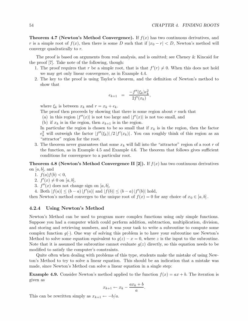
54 CHAPTER 4. FINDING ROOTS
Theorem 4.7 (Newton’s Method Convergence). If f(x) has two continuous derivatives, andr is a simple root of f(x), then there is some D such that if |x0 − r| < D, Newton’s method willconverge quadratically to r.
The proof is based on arguments from real analysis, and is omitted; see Cheney & Kincaid forthe proof [7]. Take note of the following, though:
1. The proof requires that r be a simple root, that is that f ′(r) 6= 0. When this does not holdwe may get only linear convergence, as in Example 4.4.
2. The key to the proof is using Taylor’s theorem, and the definition of Newton’s method toshow that
ek+1 =−f ′′(ξk)e2k2f ′(xk)
,
where ξk is between xk and r = xk + ek.The proof then proceeds by showing that there is some region about r such that(a) in this region |f ′′(x)| is not too large and |f ′(x)| is not too small, and(b) if xk is in the region, then xk+1 is in the region.
In particular the region is chosen to be so small that if xk is in the region, then the factore2k will outweigh the factor |f ′′(ξk)| /2 |f ′(xk)| . You can roughly think of this region as an“attractor” region for the root.
3. The theorem never guarantees that some xk will fall into the “attractor” region of a root r ofthe function, as in Example 4.5 and Example 4.6. The theorem that follows gives sufficientconditions for convergence to a particular root.
Theorem 4.8 (Newton’s Method Convergence II [2]). If f(x) has two continuous derivativeson [a, b], and
1. f(a)f(b) < 0,2. f ′(x) 6= 0 on [a, b],3. f ′′(x) does not change sign on [a, b],4. Both |f(a)| ≤ (b− a) |f ′(a)| and |f(b)| ≤ (b− a) |f ′(b)| hold,
then Newton’s method converges to the unique root of f(x) = 0 for any choice of x0 ∈ [a, b] .
4.2.4 Using Newton’s Method
Newton’s Method can be used to program more complex functions using only simple functions.Suppose you had a computer which could perform addition, subtraction, multiplication, division,and storing and retrieving numbers, and it was your task to write a subroutine to compute somecomplex function g(·). One way of solving this problem is to have your subroutine use Newton’sMethod to solve some equation equivalent to g(z)− x = 0, where z is the input to the subroutine.Note that it is assumed the subroutine cannot evaluate g(z) directly, so this equation needs to bemodified to satisfy the computer’s constraints.
Quite often when dealing with problems of this type, students make the mistake of using New-ton’s Method to try to solve a linear equation. This should be an indication that a mistake wasmade, since Newton’s Method can solve a linear equation in a single step:
Example 4.9. Consider Newton’s method applied to the function f(x) = ax+ b. The iteration isgiven as
xk+1 ← xk −axk + b
a.
This can be rewritten simply as xk+1 ← −b/a.
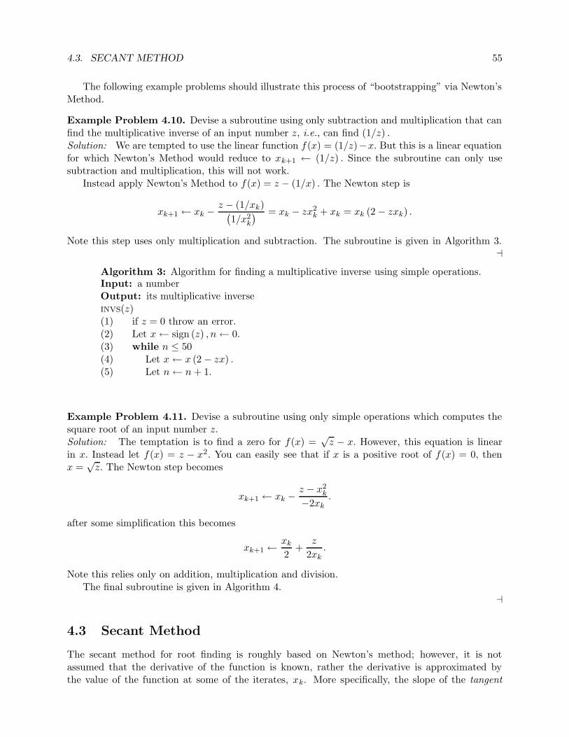
4.3. SECANT METHOD 55
The following example problems should illustrate this process of “bootstrapping” via Newton’sMethod.
Example Problem 4.10. Devise a subroutine using only subtraction and multiplication that canfind the multiplicative inverse of an input number z, i.e., can find (1/z) .Solution: We are tempted to use the linear function f(x) = (1/z)−x. But this is a linear equationfor which Newton’s Method would reduce to xk+1 ← (1/z) . Since the subroutine can only usesubtraction and multiplication, this will not work.
Instead apply Newton’s Method to f(x) = z − (1/x) . The Newton step is
xk+1 ← xk −z − (1/xk)(
1/x2k
) = xk − zx2k + xk = xk (2− zxk) .
Note this step uses only multiplication and subtraction. The subroutine is given in Algorithm 3.a
Algorithm 3: Algorithm for finding a multiplicative inverse using simple operations.Input: a numberOutput: its multiplicative inverseinvs(z)(1) if z = 0 throw an error.(2) Let x← sign (z) , n← 0.(3) while n ≤ 50(4) Let x← x (2− zx) .(5) Let n← n+ 1.
Example Problem 4.11. Devise a subroutine using only simple operations which computes thesquare root of an input number z.Solution: The temptation is to find a zero for f(x) =
√z − x. However, this equation is linear
in x. Instead let f(x) = z − x2. You can easily see that if x is a positive root of f(x) = 0, thenx =√z. The Newton step becomes
xk+1 ← xk −z − x2
k
−2xk.
after some simplification this becomes
xk+1 ←xk
2+
z
2xk.
Note this relies only on addition, multiplication and division.The final subroutine is given in Algorithm 4.
a
4.3 Secant Method
The secant method for root finding is roughly based on Newton’s method; however, it is notassumed that the derivative of the function is known, rather the derivative is approximated bythe value of the function at some of the iterates, xk. More specifically, the slope of the tangent

56 CHAPTER 4. FINDING ROOTS
Algorithm 4: Algorithm for finding a square root using simple operations.Input: a numberOutput: its square rootsqrt(z)(1) if z < 0 throw an error.(2) Let x← 1, n← 0.(3) while n ≤ 50(4) Let x← (x+ z/x) /2.(5) Let n← n+ 1.
PSfrag
replacem
ents
xk xk−1
f(xk)
f(xk−1)
xk+1f(x
k+
1 )
Figure 4.2: One iteration of the Secant method is shown for some quadratic function f(x). Thesecant line through (xk−1, f(xk−1)) and (xk, f(xk)) is shown. It happens to be the case that|f(xk+1)| is smaller than |f(xk)| , i.e., xk+1 is a better guess than xk.
line at (xk, f(xk)) , which is f ′(xk) is approximated by the slope of the secant line passing through(xk−1, f(xk−1)) and (xk, f(xk)) , which is
f(xk)− f(xk−1)
xk − xk−1
Thus the iterate xk+1 is the root of this secant line. That is, it is a root to the equation
f(xk)− f(xk−1)
xk − xk−1(x− xk) = y − f(xk).

4.3. SECANT METHOD 57
Since the root has a y value of 0, we have
f(xk)− f(xk−1)
xk − xk−1(xk+1 − xk) = −f(xk),
xk+1 − xk = −(
xk − xk−1
f(xk)− f(xk−1)
)
f(xk),
xk+1 = xk −(
xk − xk−1
f(xk)− f(xk−1)
)
f(xk). (4.2)
You will note this is the recurrence of Newton’s method, but with the slope f ′(xk) substitutedby the slope of the secant line. Note also that the secant method requires two initial guesses, x0, x1,but can be used on a black box function. The secant method can suffer from some of the sameproblems that Newton’s method does, as we will see.
An iteration of the secant method is shown in Figure 4.2, along with the secant line.
Example 4.12. Consider the secant method used on x3 + x2 − x− 1, with x0 = 2, x1 = 12 .
Note that this function is continuous and has roots ±1. We give the iterates here:
k xk f(xk)0 2 91 0.5 −1.1252 0.666666666666667 −0.9259259259259263 1.44186046511628 2.634673676531634 0.868254072087394 −0.4598424662544955 0.953491494113659 −0.1774824588768986 1.00706900811804 0.02847626921976137 0.999661272951803 −0.00135444928759928 0.999997617569723 −9.52969840528617 × 10−06
9 1.0000000008072 3.22880033820638 × 10−09
10 0.999999999999998 −7.43849426498855 × 10⁻¹⁵
4.3.1 Problems
As with Newton’s method, convergence is dependent on f(x), and the initial estimates x0, x1. Weillustrate a few possible problems:
Example 4.13. Consider the secant method for the function f(x) = lnxx , with x0 = 3, x1 = 4.
As with Newton’s method, the iterates diverge towards infinity, looking for a nonexistant root. We

58 CHAPTER 4. FINDING ROOTS
give some iterates here:
k xk f(xk)0 3 0.3662040962227031 4 0.3465735902799732 21.6548475770851 0.1420111282243413 33.9111765137635 0.1039110114416614 67.3380435135758 0.06251630044181045 117.820919458675 0.04047809049447126 210.543986613847 0.02540891658730037 366.889164762149 0.01609494192312198 637.060241341843 0.0101354060455829 1096.54125113444 0.0063836323354384710 1878.34688714646 0.0040131816999487511 3201.94672271613 0.002520814664842212 5437.69020766155 0.0015817579389472713 9203.60222260594 0.00099171498415259714 15533.1606791089 0.00062129869224134315 26149.7196085218 0.00038897525095042816 43924.8466075548 0.00024337558913788217 73636.673898472 0.000152191807070607
Example 4.14. Consider Newton’s method applied to the function f(x) = 11+x2 − 1
17 , with initialestimates x0 = −1, x1 = 1.You can easily verify that f(x0) = f(x1), and thus the secant line is horizontal. And thus x2 is notdefined.
Algorithm 5: Algorithm for finding root by secant method.Input: a function, initial guesses, an iteration limit, and a toleranceOutput: a point for which the function has small value.run secant(f, x0, x1, N, tol)(1) Let x← x1, xp← x0, fh← f(x1), fp← f(x0), n← 0.(2) while n ≤ N(3) if |fh| < tol(4) return x.(5) Let fpx← (fh− fp)/(x− xp).(6) if |fpx| < tol(7) Warn “secant slope is too small; giving up.”(8) return x.(9) Let xp← x, fp← fh.(10) Let x← x− fh/fpx.(11) Let fh← f(x).(12) Let n← n+ 1.
4.3.2 Convergence
We consider convergence analysis as in Newton’s method. We assume that r is a root of f(x), andlet en = r−xn. Because the secant method involves two iterates, we assume that we will find some
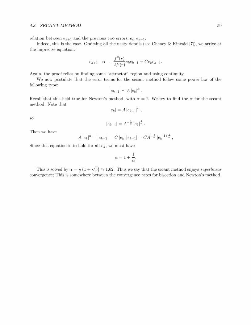
4.3. SECANT METHOD 59
relation between ek+1 and the previous two errors, ek, ek−1.Indeed, this is the case. Omitting all the nasty details (see Cheney & Kincaid [7]), we arrive at
the imprecise equation:
ek+1 ≈ − f′′(r)
2f ′(r)ekek−1 = Cekek−1.
Again, the proof relies on finding some “attractor” region and using continuity.We now postulate that the error terms for the secant method follow some power law of the
following type:|ek+1| ∼ A |ek|α .
Recall that this held true for Newton’s method, with α = 2. We try to find the α for the secantmethod. Note that
|ek| = A |ek−1|α ,so
|ek−1| = A− 1α |ek|
1α .
Then we haveA |ek|α = |ek+1| = C |ek| |ek−1| = CA− 1
α |ek|1+1α ,
Since this equation is to hold for all ek, we must have
α = 1 +1
α.
This is solved by α = 12
(
1 +√
5)
≈ 1.62. Thus we say that the secant method enjoys superlinear
convergence; This is somewhere between the convergence rates for bisection and Newton’s method.

60 CHAPTER 4. FINDING ROOTS
Exercises
(4.1) Consider the bisection method applied to find the zero of the function f(x) = x2 − 5x + 3,with a0 = 0, b0 = 1. What are a1, b1? What are a2, b2 ?
(4.2) Approximate√
10 by using two steps of Newton’s method, with an initial estimate of x0 = 3.(cf. Example Problem 4.11) Your answer should be correct to 5 decimal places.
(4.3) Consider bisection for finding the root to cos x = 0. Let the initial interval I0 be [0, 2]. Whatis the next interval considered, call it I1? What is I2? I6?
(4.4) What does the sequence defined by
x0 = 1, xk+1 =1
2xk +
1
xk
converge to?(4.5) Devise a subroutine using only simple operations that finds, via Newton’s Method, the cubed
root of some input number z.(4.6) Use Newton’s Method to approximate 3
√9. Start with x0 = 2. Find x2.
(4.7) Use Newton’s Method to devise a sequence x0, x1, . . . such that xk → ln 10. Is this a reasonableway to write a subroutine that, given z, computes ln z? (Hint: such a subroutine would requirecomputation of exk . Is this possible for rational xk without using a logarithm? Is it practical?)
(4.8) Give an example (graphical or analytic) of a function, f(x) for which Newton’s Method:(a) Does not find a root for some choices of x0.(b) Finds a root for every choice of x0.(c) Falls into a cycle for some choice of x0.(d) Converges slowly to the zero of f(x).
(4.9) How will Newton’s Method perform for finding the root to f(x) =√
|x| = 0?(4.10) Implement the inverse finder described in Example Problem 4.10. Your m-file should have
header line like:function c = invs(z)
where z is the number to be inverted. You may wish to use the builtin function sign. Asan extra termination condition, you should have the subroutine return the current iterate ifzx is sufficiently close to 1, say within the interval (0.9999, 0.0001). Can you find some z forwhich the algorithm performs poorly?
(4.11) Implement the bisection method in octave/Matlab. Your m-file should have header line like:function c = run_bisection(f, a, b, tol)
where f is the name of the function. Recall that feval(f,x) when f is a string with thename of some function evaluates that function at x. This works for builtin functions andm-files.(a) Run your code on the function f(x) = cos x, with a0 = 0, b0 = 2. In this case you can
set f = "cos".(b) Run your code on the function f(x) = x2 − 5x+ 3, with a0 = 0, b0 = 1. In this case you
will have to set f to the name of an m-file (without the “.m”) which will evaluate thegiven f(x).
(c) Run your code on the function f(x) = x− cosx, with a0 = 0, b0 = 1.(4.12) Implement Newton’s Method. Your m-file should have header line like:
function x = run_newton(f, fp, x0, N, tol)
where f is the name of the function, and fp is its derivative. Run your code to find zeroes ofthe following functions:(a) f(x) = tan x− x.
4.3. SECANT METHOD 61
(b) f(x) = x2 − (2 + ε)x+ 1 + ε, for ε small.(c) f(x) = x7 − 7x6 + 21x5 − 35x4 + 35x3 − 21x2 + 7x− 1.(d) f(x) = (x− 1)7 .
(4.13) Implement the secant method Your m-file should have header line like:function x = run_secant(f, x0, x1, N, tol)
where f is the name of the function. Run your code to find zeroes of the following functions:(a) f(x) = tan x− x.(b) f(x) = x2 + 1. (Note: This function has no zeroes.)(c) f(x) = 2 + sinx. (Note: This function also has no zeroes.)

62 CHAPTER 4. FINDING ROOTS

Chapter 5
Interpolation
5.1 Polynomial Interpolation
We consider the problem of finding a polynomial that interpolates a given set of values:
x x0 x1 . . . xn
y y0 y1 . . . yn
where the xi are all distinct. A polynomial p(x) is said to interpolate these data if p(xi) = yi fori = 0, 1, . . . , n. The xi values are called “nodes.”
Sometimes, we will consider a variant of this problem: we have some black box function, f(x),which we want to approximate with a polynomial p(x). We do this by finding the polynomialinterpolant to the data
x x0 x1 . . . xn
f(x) f(x0) f(x1) . . . f(xn)
for some choice of distinct nodes xi.
5.1.1 Lagranges Method
As you might have guessed, for any such set of data, there is an n-degree polynomial that interpo-lates it. We present a constructive proof of this fact by use of Lagrange Polynomials.
Definition 5.1 (Lagrange Polynomials). For a given set of n + 1 nodes xi, the Lagrangepolynomials are the n+ 1 polynomials `i defined by
`i(xj) = δij =
{
0 if i 6= j1 if i = j
Then we define the interpolating polynomial as
pn(x) =n∑
i=0
yi`i(x).
If each Lagrange Polynomial is of degree at most n, then pn also has this property. The LagrangePolynomials can be characterized as follows:
`i(x) =
n∏
j=0, j 6=i
x− xj
xi − xj. (5.1)
63

64 CHAPTER 5. INTERPOLATION
By evaluating this product for each xj , we see that this is indeed a characterization of the LagrangePolynomials. Moreover, each polynomial is clearly the product of n monomials, and thus has degreeno greater than n.
This gives the theorem
Theorem 5.2 (Interpolant Existence and Uniqueness). Let {xi}ni=0 be distinct nodes. Thenfor any values at the nodes, {yi}ni=0, there is exactly one polynomial, p(x) of degree no greater thann such that p(xi) = yi for i = 0, 1, . . . , n.
Proof. The Lagrange Polynomial construction gives existence of such a polynomial p(x) of degreeno greater than n.
Suppose there were two such polynomials, call them p(x), q(x), each of degree no greater thann, both interpolating the data. Let r(x) = p(x)− q(x). Note that r(x) can have degree no greaterthan n, yet it has roots at x0, x1, . . . , xn. The only polynomial of degree ≤ n that has n+1 distinctroots is the zero polynomial, i.e., 0 ≡ r(x) = p(x) − q(x). Thus p(x), q(x) are equal everywhere,i.e., they are the same polynomial.
Example Problem 5.3. Construct the polynomial interpolating the data
x 1 12 3
y 3 −10 2
by using Lagrange Polynomials.Solution: We construct the Lagrange Polynomials:
`0(x) =(x− 1
2)(x− 3)
(1− 12)(1− 3)
= −(x− 1
2)(x− 3)
`1(x) =(x− 1)(x− 3)
(12 − 1)(1
2 − 3)=
4
5(x− 1)(x − 3)
`2(x) =(x− 1)(x− 1
2)
(3− 1)(3 − 12 )
=1
5(x− 1)(x− 1
2)
Then the interpolating polynomial, in “Lagrange Form” is
p2(x) = −3(x− 1
2)(x− 3)− 8(x− 1)(x− 3) +
2
5(x− 1)(x− 1
2)
a
5.1.2 Newton’s Method
There is another way to prove existence. This method is also constructive, and leads to a differentalgorithm for constructing the interpolant. One way to view this construction is to imagine howone would update the Lagrangian form of an interpolant. That is, suppose some data were given,and the interpolating polynomial calculated using Lagrange Polynomials; then a new point wasgiven (xn+1, yn+1), and an interpolant for the augmented set of data is to be found. Each LagrangePolynomial would have to be updated. This could take a lot of calculation (especially if n is large).
So the alternative method constructs the polynomials iteratively. Thus we create polynomialspk(x) such that pk(xi) = yi for 0 ≤ i ≤ k. This is simple for k = 0, we simply let
p0(x) = y0,
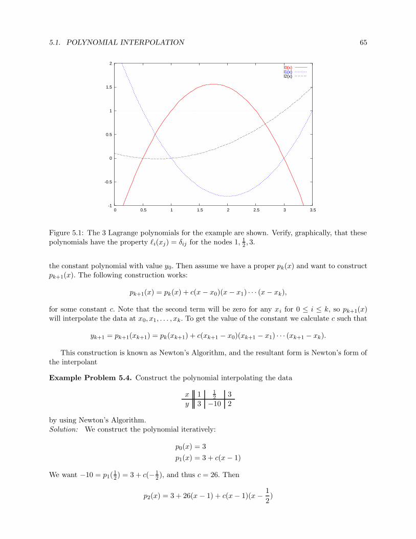
5.1. POLYNOMIAL INTERPOLATION 65
-1
-0.5
0
0.5
1
1.5
2
0 0.5 1 1.5 2 2.5 3 3.5
l0(x)l1(x)l2(x)
Figure 5.1: The 3 Lagrange polynomials for the example are shown. Verify, graphically, that thesepolynomials have the property `i(xj) = δij for the nodes 1, 1
2 , 3.
the constant polynomial with value y0. Then assume we have a proper pk(x) and want to constructpk+1(x). The following construction works:
pk+1(x) = pk(x) + c(x− x0)(x− x1) · · · (x− xk),
for some constant c. Note that the second term will be zero for any xi for 0 ≤ i ≤ k, so pk+1(x)will interpolate the data at x0, x1, . . . , xk. To get the value of the constant we calculate c such that
yk+1 = pk+1(xk+1) = pk(xk+1) + c(xk+1 − x0)(xk+1 − x1) · · · (xk+1 − xk).
This construction is known as Newton’s Algorithm, and the resultant form is Newton’s form ofthe interpolant
Example Problem 5.4. Construct the polynomial interpolating the data
x 1 12 3
y 3 −10 2
by using Newton’s Algorithm.Solution: We construct the polynomial iteratively:
p0(x) = 3
p1(x) = 3 + c(x− 1)
We want −10 = p1(12) = 3 + c(− 1
2 ), and thus c = 26. Then
p2(x) = 3 + 26(x − 1) + c(x− 1)(x − 1
2)

66 CHAPTER 5. INTERPOLATION
-35
-30
-25
-20
-15
-10
-5
0
5
10
15
0 0.5 1 1.5 2 2.5 3 3.5 4
p(x)
Figure 5.2: The interpolating polynomial for the example is shown.
We want 2 = p2(3) = 3 + 26(2) + c(2)( 52 ), and thus c = −53
5 . Then we get
p2(x) = 3 + 26(x− 1) +−53
5(x− 1)(x− 1
2).
aDoes Newton’s Algorithm give a different polynomial? It is easy to show, by induction, that
the degree of pn(x) is no greater than n. Then, by Theorem 5.2, it must be the same polynomialas the Lagrange interpolant.
The two methods give the same interpolant, we may wonder “Which should we use?” Newton’sAlgorithm seems more flexible–it can deal with adding new data. There also happens to be a wayof storing Newton’s form of the interpolant that makes the polynomial simple to evaluate (in thesense of number of calculations required).
5.1.3 Newton’s Nested Form
Recall the iterative construction of Newton’s Form:
pk+1(x) = pk(x) + ck(x− x0)(x− x1) · · · (x− xk).
The previous iterate pk(x) was constructed similarly, so we can write:
pk+1(x) = [pk−1(x) + ck−1(x− x0)(x− x1) · · · (x− xk−1)] + ck(x− x0)(x− x1) · · · (x− xk).
Continuing in this way we see that we can write
pn(x) =
n∑
k=0
ck
∏
0≤j<k
(x− xj)
, (5.2)
where an empty product has value 1 by convention. This can be rewritten in a funny form, wherea monomial is factored out of each successive summand:
pn(x) = c0 + (x− x0)[c1 + (x− x1)[c2 + (x− x2) [. . .]]]

5.1. POLYNOMIAL INTERPOLATION 67
Supposing for an instant that the constants ck were known, this provides a better way ofcalculating pn(t) at arbitrary t. By “better” we mean requiring few multiplications and additions.This nested calculation is performed iteratively:
v0 = cn
v1 = cn−1 + (t− xn−1)v0
v2 = cn−2 + (t− xn−2)v1...
vn = c0 + (t− x0)vn−1
This requires only n multiplications and 2n additions. Compare this with the number requiredfor using the Lagrange form: at least n2 additions and multiplications.
5.1.4 Divided Differences
It turns out that the coefficients ck for Newton’s nested form can be calculated relatively easily byusing divided differences. We assume, for the remainder of this section, that we are consideringinterpolating a function, that is, we have values of f(xi) at the nodes xi.
Definition 5.5 (Divided Differences). For a given collection of nodes {xi}ni=0 and values{f(xi)}nx=0, a kth order divided difference is a function of k + 1 (not necessarily distinct) nodes,written as
f [xi0 , xi1 , . . . , xik ]
The divided differences are defined recursively as follows:
• The 0th order divided differences are simply defined:
f [xi] = f(xi).
• Higher order divided differences are the ratio of differences:
f [xi0 , xi1 , . . . , xik ] =f [xi1 , xi2 , . . . , xik ]− f
[
xi0 , xi1 , . . . , xik−1
]
xik − xi0
We care about divided differences because coefficients for the Newton nested form are divideddifferences:
ck = f [x0, x1, . . . , xk] . (5.3)
Because we are only interested in the Newton method coefficients, we will only consider divideddifferences with successive nodes, i.e., those of the form f [xj, xj+1, . . . , xj+k]. In this case thehigher order differences can more simply be written as
f [xj , xj+1, . . . , xj+k] =f [xj+1, xj+2, . . . , xj+k]− f [xj, xj+1, . . . , xj+k−1]
xj+k − xj

68 CHAPTER 5. INTERPOLATION
The graphical way to calculate these things is a “pyramid scheme”1, where you compute thefollowing table columnwise, from left to right:
x f [ ] f [ , ] f [ , , ] f [ , , , ]
x0 f [x0]f [x0, x1]
x1 f [x1] f [x0, x1, x2]f [x1, x2] f [x0, x1, x2, x3]
x2 f [x2] f [x1, x2, x3]f [x2, x2]
x3 f [x3]
Note that by definition, the first column just echoes the data: f [xi] = f(xi).We drag out our example one last time:
Example Problem 5.6. Find the divided differences for the following data
x 1 12 3
f(x) 3 −10 2
Solution: We start by writing in the data:
x f [ ] f [ , ] f [ , , ]
1 3
12 −10
3 2
Then we calculate:
f [x0, x1] =−10− 3
(1/2) − 1= 26, and f [x1, x2] =
2−−10
3− (1/2)= 24/5.
Adding these to the table, we have
x f [ ] f [ , ] f [ , , ]
1 326
12 −10
245
3 2
Then we calculate
f [x0, x1, x2] =24/5 − 26
3− 1=−53
5.
So we complete the table:x f [ ] f [ , ] f [ , , ]
1 326
12 −10 −53
5245
3 2
1That’s supposed to be a joke.

5.2. ERRORS IN POLYNOMIAL INTERPOLATION 69
You should verify that along the top line of this pyramid you can read off the coefficients forNewton’s form, as found in Example Problem 5.4. a
5.2 Errors in Polynomial Interpolation
We now consider two questions:
1. If we want to interpolate some function f(x) at n + 1 nodes over some closed interval, howshould we pick the nodes?
2. How accurate can we make a polynomial interpolant over a closed interval?
You may be surprised to find that the answer to the first question is not that we should makethe xi equally spaced over the closed interval, as the following example illustrates.
Example 5.7 (Runge Function). Let
f(x) =(
1 + x2)−1
,
(known as the Runge Function), and let pn(x) interpolate f on n equally spaced nodes, includingthe endpoints, on [−5, 5]. Then
limn→∞
maxx∈[−5,5]
|pn(x)− f(x)| =∞.
This behaviour is shown in Figure 5.3.
It turns out that a much better choice is related to the Chebyshev Polynomials (“of the firstkind”). If our closed interval is [−1, 1], then we want to define our nodes as
xi = cos
[(
2i+ 1
2n+ 2
)
π
]
, 0 ≤ i ≤ n.
Literally interpreted, these Chebyshev Nodes are the projections of points uniformly spaced ona semi circle; see Figure 5.4. By using the Chebyshev nodes, a good polynomial interpolant of theRunge function of Example 5.7 can be found, as shown in Figure 5.5.
5.2.1 Interpolation Error Theorem
We did not just invent the Chebyshev nodes. The fact that they are “good” for interpolationfollows from the following theorem:
Theorem 5.8 (Interpolation Error Theorem). Let p be the polynomial of degree at most ninterpolating function f at the n+1 distinct nodes x0, x1, . . . , xn on [a, b]. Let f (n+1) be continuous.Then for each x ∈ [a, b] there is some ξ ∈ [a, b] such that
f(x)− p(x) =1
(n+ 1)!f (n+1)(ξ)
n∏
i=0
(x− xi) .
You should be thinking that the term on the right hand side resembles the error term in Taylor’sTheorem.

70 CHAPTER 5. INTERPOLATION
-0.4
-0.2
0
0.2
0.4
0.6
0.8
1
-6 -4 -2 0 2 4 6
runge3 nodes7 nodes
10 nodes
(a) 3,7,10 equally spaced nodes
-1
0
1
2
3
4
5
6
7
8
-6 -4 -2 0 2 4 6
runge15 nodes
(b) 15 equally spaced nodes
-700000
-600000
-500000
-400000
-300000
-200000
-100000
0
100000
-6 -4 -2 0 2 4 6
runge50 nodes
(c) 50 equally spaced nodes
Figure 5.3: The Runge function is poorly interpolated at n equally spaced nodes, as n gets large.At first, the interpolations appear to improve with larger n, as in (a). In (b) it becomes apparentthat the interpolant is good in center of the interval, but bad at the edges. As shown in (c), thisgets worse as n gets larger.

5.2. ERRORS IN POLYNOMIAL INTERPOLATION 71
bottomright
topleft
PSfrag
replacem
ents
11−
Figure 5.4: The Chebyshev nodes are the projections of nodes equally spaced on a semi circle.
-0.4
-0.2
0
0.2
0.4
0.6
0.8
1
-6 -4 -2 0 2 4 6
runge3 nodes7 nodes
10 nodes
(a) 3,7,10 Chebyshev nodes
0
0.1
0.2
0.3
0.4
0.5
0.6
0.7
0.8
0.9
1
-6 -4 -2 0 2 4 6
runge17 nodes
(b) 17 Chebyshev nodes
Figure 5.5: The Chebyshev nodes yield good polynomial interpolants of the Runge function. Com-pare these figures to those of Figure 5.3. For more than about 25 nodes, the interpolant is indis-tinguishable from the Runge function by eye.
Proof. First consider when x is one of the nodes xi; in this case both the LHS and RHS are zero.So assume x is not a node. Make the following definitions
w(t) =
n∏
i=0
(t− xi) ,
c =f(x)− p(x)
w(x),
φ(t) = f(t)− p(t)− cw(t).
Since x is not a node, w(x) is nonzero. Now note that φ(xi) is zero for each node xi, and that bydefinition of c, that φ(x) = 0 for our x. That is φ(t) has n+ 2 roots.
Some other facts: f, p, w have n+ 1 continuous derivatives, by assumption and definition; thusφ has this many continuous derivatives. Apply Rolle’s Theorem to φ(t) to find that φ ′(t) has n+ 1

72 CHAPTER 5. INTERPOLATION
roots. Then apply Rolle’s Theorem again to find φ′′(t) has n roots. In this way we see that φ(n+1)(t)has a root, call it ξ. That is
0 = φ(n+1)(ξ) = f (n+1)(ξ)− p(n+1)(ξ)− cw(n+1)(ξ).
But p(t) is a polynomial of degree ≤ n, so p(n+1) is identically zero. And w(t) is a polynomialof degree n+ 1 in t, so its n+ 1th derivative is easily seen to be (n+ 1)! Thus
0 = f (n+1)(ξ)− c(n+ 1)!
c(n+ 1)! = f (n+1)(ξ)
f(x)− p(x)w(x)
=1
(n+ 1)!f (n+1)(ξ)
f(x)− p(x) =1
(n+ 1)!f (n+1)(ξ)w(x),
which is what was to be proven.
Thus the error in a polynomial interpolation is given as
f(x)− p(x) =1
(n+ 1)!f (n+1)(ξ)
n∏
i=0
(x− xi) .
We have no control over the function f(x) or its derivatives, and once the nodes and f are fixed, pis determined; thus the only way we can make the error |f(x)− p(x)| small is by judicious choiceof the nodes xi.
The Chebyshev nodes on [−1, 1] have the remarkable property that∣
∣
∣
∣
∣
n∏
i=0
(t− xi)
∣
∣
∣
∣
∣
≤ 2−n
for any t ∈ [−1, 1] . Moreover, it can be shown that for any choice of nodes xi that
maxt∈[−1,1]
∣
∣
∣
∣
∣
n∏
i=0
(t− xi)
∣
∣
∣
∣
∣
≥ 2−n.
Thus the Chebyshev nodes are considered the best for polynomial interpolation.Merging this result with Theorem 5.8, the error for polynomial interpolants defined on Cheby-
shev nodes can be bounded as
|f(x)− p(x)| ≤ 1
2n (n+ 1)!max
ξ∈[−1,1]
∣
∣
∣f (n+1)(ξ)∣
∣
∣ .
The Chebyshev nodes can be rescaled and shifted for use on the general interval [α, β]. In thiscase they take the form
xi =β − α
2cos
[(
2i+ 1
2n+ 2
)
π
]
+α+ β
2, 0 ≤ i ≤ n.
In this case, the rescaling of the nodes changes the bound on∏
(t− xi) so the overall error boundbecomes
|f(x)− p(x)| ≤ (β − α)n+1
22n+1 (n+ 1)!max
ξ∈[α,β]
∣
∣
∣f (n+1)(ξ)∣
∣
∣ ,
for x ∈ [α, β] .

5.2. ERRORS IN POLYNOMIAL INTERPOLATION 73
Example Problem 5.9. How many Chebyshev nodes are required to interpolate the functionf(x) = sin(x) + cos(x) to within 10−8 on the interval [0, π]?Solution: We first find the derivatives of f
f ′(x) = cos(x)− sin(x)
f ′′(x) = − sin(x)− cos(x)
f ′′′(x) = − cos(x) + sin(x)
...
As a crude approximation we can assert that
∣
∣
∣f (k)(x)
∣
∣
∣≤ |cosx|+ |sinx| ≤ 2.
Thus it suffices to take n large enough such that
πn+1
22n+1 (n+ 1)!2 ≤ 10−8
By trial and error we see that n = 10 suffices. a
5.2.2 Interpolation Error for Equally Spaced Nodes
Despite the proven superiority of Chebyshev Nodes, and the problems with the Runge Function,equally spaced nodes are frequently used for interpolation, since they are easy to calculate2. Wenow consider bounding
maxx∈[a,b]
n∏
i=0
|x− xi| ,
where
xi = a+ hi = a+(b− a)n
i, i = 0, 1, . . . , n.
Start by picking an x. We can assume x is not one of the nodes, otherwise the product inquestion is zero. Then x is between some xj , xj+1 We can show that
|x− xj| |x− xj+1| ≤h2
4.
by simple calculus.Now we claim that |x− xi| ≤ (j − i+ 1) h for i < j, and |x− xi| ≤ (i− j) h for j +1 < i. Then
n∏
i=0
|x− xi| ≤h2
4
[
(j + 1)!hj] [
(n− j)!hn−j−1]
.
It can be shown that (j + 1)!(n− j)! ≤ n!, and so we get an overall bound
n∏
i=0
|x− xi| ≤hn+1n!
4.
2Never underestimate the power of laziness.

74 CHAPTER 5. INTERPOLATION
The interpolation theorem then gives us
|f(x)− p(x)| ≤ hn+1
4 (n+ 1)maxξ∈[a,b]
∣
∣
∣f (n+1)(ξ)∣
∣
∣ ,
where h = (b− a)/n.The reason this result does not seem to apply to Runge’s Function is that f (n) for Runge’s
Function becomes unbounded as n→∞.
Example Problem 5.10. How many equally spaced nodes are required to interpolate the functionf(x) = sin(x) + cos(x) to within 10−8 on the interval [0, π]?Solution: As in Example Problem 5.9, we make the crude approximation
∣
∣
∣f (k)(x)
∣
∣
∣≤ |cosx|+ |sinx| ≤ 2.
Thus we want to make n sufficiently large such that
hn+1
4(n+ 1)2 ≤ 10−8,
where h = (π − 0)/n. That is we want to find n large enough such that
πn+1
2nn+1(n+ 1)≤ 10−8,
By simply trying small numbers, we can see this is satisfied if n = 12. a
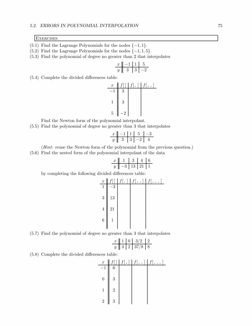
5.2. ERRORS IN POLYNOMIAL INTERPOLATION 75
Exercises
(5.1) Find the Lagrange Polynomials for the nodes {−1, 1}.(5.2) Find the Lagrange Polynomials for the nodes {−1, 1, 5}.(5.3) Find the polynomial of degree no greater than 2 that interpolates
x −1 1 5
y 3 3 −2
(5.4) Complete the divided differences table:
x f [ ] f [ , ] f [ , , ]
−1 3
1 3
5 −2
Find the Newton form of the polynomial interpolant.(5.5) Find the polynomial of degree no greater than 3 that interpolates
x −1 1 5 −3
y 3 3 −2 4
(Hint: reuse the Newton form of the polynomial from the previous question.)(5.6) Find the nested form of the polynomial interpolant of the data
x 1 3 4 6
y −3 13 21 1
by completing the following divided differences table:
x f [ ] f [ , ] f [ , , ] f [ , , , ]
1 −3
3 13
4 21
6 1
(5.7) Find the polynomial of degree no greater than 3 that interpolates
x 1 0 3/2 2
y 3 2 37/8 8
(5.8) Complete the divided differences table:
x f [ ] f [ , ] f [ , , ] f [ , , , ]
−1 6
0 3
1 2
2 3

76 CHAPTER 5. INTERPOLATION
(Something a little odd should have happened in the last column.) Find the Newton form ofthe polynomial interpolant. Of what degree is the polynomial interpolant?
(5.9) Let p(x) interpolate the function cos(x) at n equally spaced nodes on the interval [0, 2]. Boundthe error
max0≤x≤2
|p(x)− cos(x)|
as a function of n. How small is the error when n = 10? How small would the error be ifChebyshev nodes were used instead? How about when n = 10?
(5.10) Let p(x) interpolate the function x−2 at n equally spaced nodes on the interval [0.5, 1].Bound the error
max0.5≤x≤1
∣
∣p(x)− x−2∣
∣
as a function of n. How small is the error when n = 10?(5.11) How many Chebyshev nodes are required to interpolate the function 1
x to within 10−6 onthe interval [1, 2]?
(5.12) Write code to calculate the Newton form coefficients, by divided differences, for the nodesxi and values f(xi). Your m-file should have header line like:function coefs = newtonCoef(xs,fxs)
where xs is the vector of n+ 1 nodes, and fxs the vector of n+ 1 values. Test your code onthe following input:octave:1> xs = [1 -1 2 -2 3 -3 4 -4];
octave:2> fxs = [1 1 2 3 5 8 13 21];
octave:3> newtonCoef(xs,fxs)
ans =
1.00000 -0.00000 0.33333 -0.08333 0.05000 0.00417 -0.00020 -0.00040
(a) What do you get when you try the following?octave:4> xs = [1 4 5 9 14 23 37 60];
octave:5> fxs = [3 1 4 1 5 9 2 6];
octave:6> newtonCoef(xs,ys)
(b) Try the following:octave:7> xs = [1 3 4 2 8 -2 0 14 23 15];
octave:8> fxs = xs.*xs + xs .+ 4;
octave:9> newtonCoef(xs,fxs)
(5.13) Write code to calculate a polynomial interpolant from its Newton form coefficients and thenode values. Your m-file should have header line like:function y = calcNewton(t,coefs,xs)
where coefs is a vector of the Newton coefficients, xs is a vector of the nodes xi, and y isthe value of the interpolating polynomial at t. Check your code against the following values:octave:1> xs = [1 3 4];
octave:2> coefs = [6 5 1];
octave:3> calcNewton (5,coefs,xs)
ans = 34
octave:4> calcNewton (-3,coefs,xs)
ans = 10
(a) What do you get when you try the following?octave:5> xs = [3 1 4 5 9 2 6 8 7 0];

5.2. ERRORS IN POLYNOMIAL INTERPOLATION 77
octave:6> coefs = [1 -1 2 -2 3 -3 4 -4 5 -5];
octave:7> calcNewton(0.5,coefs,xs)
(b) Try the followingoctave:8> xs = [3 1 4 5 9 2 6 8 7 0];
octave:9> coefs = [1 -1 2 -2 3 -3 4 -4 5 -5];
octave:10> calcNewton(1,coefs,xs)

78 CHAPTER 5. INTERPOLATION
Chapter 6
Spline Interpolation
Splines are used to approximate complex functions and shapes. A spline is a function consisting ofsimple functions glued together. In this way a spline is different from a polynomial interpolation,which consists of a single well defined function that approximates a given shape; splines are normallypiecewise polynomial.
6.1 First and Second Degree Splines
Splines make use of partitions, which are a way of cutting an interval into a number of subintervals.
Definition 6.1 (Partition). A partition of the interval [a, b] is an ordered sequence {ti}ni=0 suchthat
a = t0 < t1 < · · · < tn−1 < tn = b
The numbers ti are known as knots.
A spline of degree 1, also known as a linear spline, is a function which is linear on each subintervaldefined by a partition:
Definition 6.2 (Linear Splines). A function S is a spline of degree 1 on [a, b] if1. The domain of S is [a, b].2. S is continuous on [a, b].3. There is a partition {ti}ni=0 of [a, b] such that on each [ti, ti+1], S is a linear polynomial.
A linear spline is defined entirely by its value at the knots. That is, given
t t0 t1 . . . tny y0 y1 . . . yn
there is only one linear spline with these values at the knots and linear on each given subinterval.For a spline with this data, the linear polynomial on each subinterval is defined as
Si(x) = yi +yi+1 − yi
ti+1 − ti(x− ti) .
Note that if x ∈ [ti, ti+1] , then x − ti > 0, but x − ti−1 ≤ 0. Thus if we wish to evaluate S(x), wesearch for the largest i such that x− ti > 0, then evaluate Si(x).
Example 6.3. The linear spline for the following data
t 0.0 0.1 0.4 0.5 0.75 1.0
y 1.3 4.5 2.0 2.1 5.0 3
is shown in Figure 6.1.
79

80 CHAPTER 6. SPLINE INTERPOLATION
0
1
2
3
4
5
6
0 0.2 0.4 0.6 0.8 1
Figure 6.1: A linear spline. The spline is piecewise linear, and is linear between each knot.
6.1.1 First Degree Spline Accuracy
As with polynomial functions, splines are used to interpolate tabulated data as well as functions. Inthe latter case, if the spline is being used to interpolate the function f, say, then this is equivalentto interpolating the data
t t0 t1 . . . tny f(t0) f(t1) . . . f(tn)
A function and its linear spline interpolant are shown in Figure 6.2. The spline interpolant inthat figure is fairly close to the function over some of the interval in question, but it also deviatesgreatly from the function at other points of the interval. We are interested in finding bounds onthe possible error between a function and its spline interpolant.
To find the error bound, we will consider the error on a single interval of the partition, and usea little calculus.1 Suppose p(t) is the linear polynomial interpolating f(t) at the endpoints of thesubinterval [ti, ti+1], then for t ∈ [ti, ti+1] ,
|f(t)− p(t)| ≤ max {|f(t)− f(ti)| , |f(t)− f(ti+1)|} .
That is, |f(t)− p(t)| is no larger than the “maximum variation” of f(t) on this interval.
In particular, if f ′(t) exists and is bounded by M1 on [ti, ti+1], then
|f(t)− p(t)| ≤ M1
2(ti+1 − ti) .
Similarly, if f ′′(t) exists and is bounded by M2 on [ti, ti+1], then
|f(t)− p(t)| ≤ M2
8(ti+1 − ti)2 .
Over a given partition, these become, respectively
1Although we could directly claim Theorem 5.8, it is a bit of overkill.
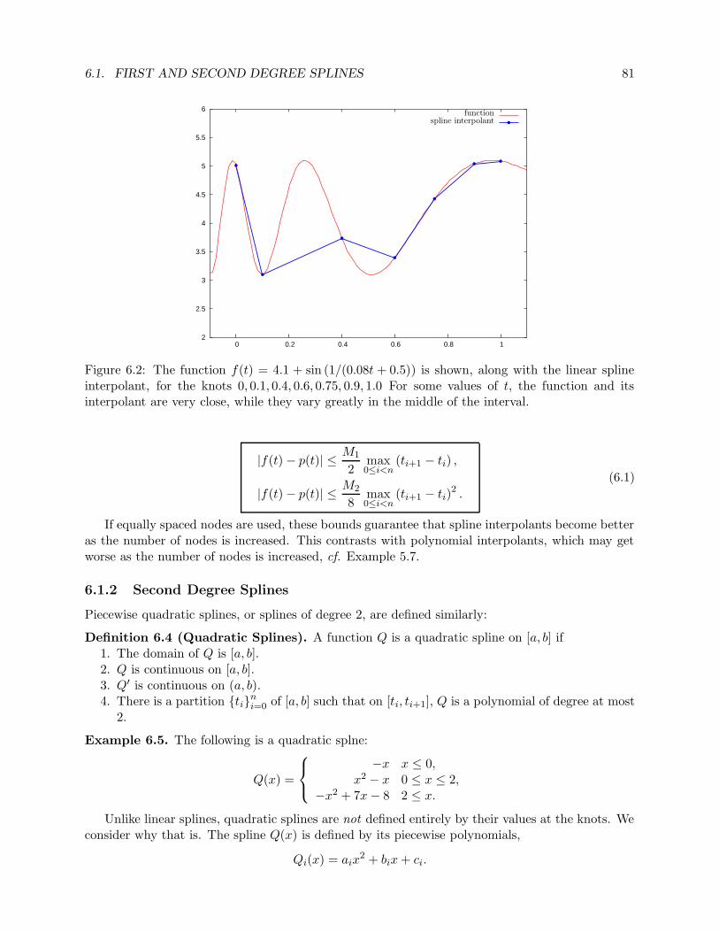
6.1. FIRST AND SECOND DEGREE SPLINES 81
2
2.5
3
3.5
4
4.5
5
5.5
6
0 0.2 0.4 0.6 0.8 1
PSfrag
replacem
ents
functionspline interpolant
Figure 6.2: The function f(t) = 4.1 + sin (1/(0.08t + 0.5)) is shown, along with the linear splineinterpolant, for the knots 0, 0.1, 0.4, 0.6, 0.75, 0.9, 1.0 For some values of t, the function and itsinterpolant are very close, while they vary greatly in the middle of the interval.
|f(t)− p(t)| ≤ M1
2max0≤i<n
(ti+1 − ti) ,
|f(t)− p(t)| ≤ M2
8max0≤i<n
(ti+1 − ti)2 .(6.1)
If equally spaced nodes are used, these bounds guarantee that spline interpolants become betteras the number of nodes is increased. This contrasts with polynomial interpolants, which may getworse as the number of nodes is increased, cf. Example 5.7.
6.1.2 Second Degree Splines
Piecewise quadratic splines, or splines of degree 2, are defined similarly:
Definition 6.4 (Quadratic Splines). A function Q is a quadratic spline on [a, b] if1. The domain of Q is [a, b].2. Q is continuous on [a, b].3. Q′ is continuous on (a, b).4. There is a partition {ti}ni=0 of [a, b] such that on [ti, ti+1], Q is a polynomial of degree at most
2.
Example 6.5. The following is a quadratic splne:
Q(x) =
−x x ≤ 0,x2 − x 0 ≤ x ≤ 2,
−x2 + 7x− 8 2 ≤ x.Unlike linear splines, quadratic splines are not defined entirely by their values at the knots. We
consider why that is. The spline Q(x) is defined by its piecewise polynomials,
Qi(x) = aix2 + bix+ ci.

82 CHAPTER 6. SPLINE INTERPOLATION
Thus there are 3n parameters to define Q(x).For each of the n subintervals, the data
t t0 t1 . . . tny y0 y1 . . . yn
give two equations regarding Qi(x), namely that Qi(ti) must equal yi and Qi(ti+1) must equal yi+1.This is 2n equations. The condition on continuity of Q′ gives a single equation for each of the n−1internal nodes. This totals 3n− 1 equations, but 3n unknowns. This system is underdetermined.
Thus some additional user-chosen condition is required to determine the quadratic spline. Onemight choose, for example, Q′(a) = 0, or Q′′(a) = 0, or some other condition.
6.1.3 Computing Second Degree Splines
Suppose the datat t0 t1 . . . tny y0 y1 . . . yn
are given. Let zi = Q′i(ti), and suppose that the additional condition to define the quadratic spline
is given by specifying z0. We want to be able to compute the form of Qi(x).Because Qi(ti) = yi, Q
′i(ti) = zi, Q
′i(ti+1) = zi+1, we see that we can define
Qi(x) =zi+1 − zi
2 (ti+1 − ti)(x− ti)2 + zi (x− ti) + yi.
Use this at ti+1 :
yi+1 = Qi(ti+1) =zi+1 − zi
2 (ti+1 − ti)(ti+1 − ti)2 + zi (ti+1 − ti) + yi,
yi+1 − yi =zi+1 − zi
2(ti+1 − ti) + zi (ti+1 − ti) ,
yi+1 − yi =zi+1 + zi
2(ti+1 − ti) .
Thus we can determine, from the data alone, zi+1 from zi:
zi+1 = 2yi+1 − yi
ti+1 − ti− zi.
6.2 (Natural) Cubic Splines
If you recall the definition of the linear and quadratic splines, probably you can guess the definitionof the spline of degree k:
Definition 6.6 (Splines of Degree k). A function S is a spline of degree k on [a, b] if1. The domain of S is [a, b].2. S, S′, S′′, . . . , S(k−1) are continuous on (a, b).3. There is a partition {ti}ni=0 of [a, b] such that on [ti, ti+1], S is a polynomial of degree ≤ k.You would also expect that a spline of degree k has k − 1 “degrees of freedom,” as we show
here. If the partition has n+1 knots, the spline of degree k is defined by n(k+1) parameters. Thegiven data
t t0 t1 . . . tny y0 y1 . . . yn

6.2. (NATURAL) CUBIC SPLINES 83
provide 2n equations. The continuity of S ′, S′′, . . . , S(k−1) at the n − 1 internal knots gives (k −1)(n − 1) equations. This is a total of n(k + 1) − (k − 1) equations. Thus we have k − 1 moreunknowns than equations. Thus, barring some singularity, we can (and must) add k−1 constraintsto uniquely define the spline. These are the degrees of freedom.
Often k is chosen as 3. This yields cubic splines. We must add 2 extra constraints to define thespline. The usual choice is to make
S′′(t0) = S′′(tn) = 0.
This yields the natural cubic spline.
6.2.1 Why Natural Cubic Splines?
It turns out that natural cubic splines are a good choice in the sense that they are the “inter-polant of minimal H2 seminorm.” The corollary following this theorem states this in more easilyunderstandable terms:
Theorem 6.7. Suppose f has two continuous derivatives, and S is the natural cubic spline inter-polating f at knots a = t0 < t1 < . . . < tn = b. Then
∫ b
a
[
S′′(x)]2
dx ≤∫ b
a
[
f ′′(x)]2
dx
Proof. We let g(x) = f(x)− S(x). Then g(x) is zero on the (n+ 1) knots ti. Derivatives are linear,meaning that
f ′′(x) = S′′(x) + g′′(x).
Then∫ b
a
[
f ′′(x)]2
dx =
∫ b
a
[
S′′(x)]2
dx+
∫ b
a
[
g′′(x)]2
dx+
∫ b
a2S′′(x)g′′(x) dx.
We show that the last integral is zero. Integrating by parts we get
∫ b
aS′′(x)g′′(x) dx = S′′g′
∣
∣
∣
b
a−∫ b
aS′′′g′ dx = −
∫ b
aS′′′g′ dx,
because S ′′(a) = S′′(b) = 0. Then notice that S is a polynomial of degree ≤ 3 on each interval, thusS′′′(x) is a piecewise constant function, taking value ci on each interval [ti, ti+1]. Thus
∫ b
aS′′′g′ dx =
n−1∑
i=0
∫ b
acig
′ dx =n−1∑
i=0
cig∣
∣
∣
ti+1
ti= 0,
with the last equality holding because g(x) is zero at the knots.
Corollary 6.8. The natural cubic spline is best twice-continuously differentiable interpolant for atwice-continuously differentiable function, under the measure given by the theorem.
Proof. Let f be twice-continuously differentiable, and let S be the natural cubic spline interpolatingf(x) at some given nodes {ti}ni=0. Let R(x) be some twice-continuously differentiable functionwhich also interpolates f(x) at these nodes. Then S(x) interpolates R(x) at these nodes. Applythe theorem to get
∫ b
a
[
S′′(x)]2
dx ≤∫ b
a
[
R′′(x)]2
dx
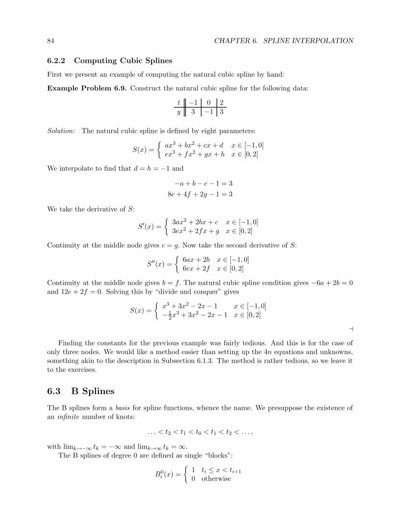
84 CHAPTER 6. SPLINE INTERPOLATION
6.2.2 Computing Cubic Splines
First we present an example of computing the natural cubic spline by hand:
Example Problem 6.9. Construct the natural cubic spline for the following data:
t −1 0 2
y 3 −1 3
Solution: The natural cubic spline is defined by eight parameters:
S(x) =
{
ax3 + bx2 + cx+ d x ∈ [−1, 0]ex3 + fx2 + gx+ h x ∈ [0, 2]
We interpolate to find that d = h = −1 and
−a+ b− c− 1 = 3
8e+ 4f + 2g − 1 = 3
We take the derivative of S:
S′(x) =
{
3ax2 + 2bx+ c x ∈ [−1, 0]3ex2 + 2fx+ g x ∈ [0, 2]
Continuity at the middle node gives c = g. Now take the second derivative of S:
S′′(x) =
{
6ax+ 2b x ∈ [−1, 0]6ex+ 2f x ∈ [0, 2]
Continuity at the middle node gives b = f. The natural cubic spline condition gives −6a+ 2b = 0and 12e+ 2f = 0. Solving this by “divide and conquer” gives
S(x) =
{
x3 + 3x2 − 2x− 1 x ∈ [−1, 0]−1
2x3 + 3x2 − 2x− 1 x ∈ [0, 2]
a
Finding the constants for the previous example was fairly tedious. And this is for the case ofonly three nodes. We would like a method easier than setting up the 4n equations and unknowns,something akin to the description in Subsection 6.1.3. The method is rather tedious, so we leave itto the exercises.
6.3 B Splines
The B splines form a basis for spline functions, whence the name. We presuppose the existence ofan infinite number of knots:
. . . < t2 < t1 < t0 < t1 < t2 < . . . ,
with limk→−∞ tk = −∞ and limk→∞ tk =∞.The B splines of degree 0 are defined as single “blocks”:
B0i (x) =
{
1 ti ≤ x < ti+1
0 otherwise

6.3. B SPLINES 85
The zero degree B splines are continuous from the right, are nonzero only on one subinterval[ti, ti+1), sum to 1 everywhere.
We justify the description of B splines as basis splines: If S is a spline of degree 0 on the givenknots and is continuous from the right then
S(x) =∑
i
S(xi)B0i (x).
That is, the basis splines work in the same way that Lagrange Polynomials worked for polynomialinterpolation.
The B splines of degree k are defined recursively:
Bki (x) =
(
x− titi+k − ti
)
Bk−1i (x) +
(
ti+k+1 − xti+k+1 − ti+1
)
Bk−1i+1 (x).
Some B splines are shown in Figure 6.3.The B splines quickly become unwieldy. We focus on the case k = 1. The B spline B 1
i (x) is• Piecewise linear.• Continuous.• Nonzero only on (ti, ti+2).• 1 at ti+1.
These B splines are sometimes called hat functions. Imagine wearing a hat shaped like this! What-ever.
The nice thing about the hat functions is they allow us to use analogy. Harken back to polyno-mial interpolation and the Lagrange Functions. The hat functions play a similar role because
B1i (tj) = δ(i+1)j =
{
1 (i+ 1) = j0 (i+ 1) 6= j
Then if we want to interpolate the following data with splines of degree 1:
t t0 t1 . . . tny y0 y1 . . . yn
We can immediately set
S(x) =
n∑
i=0
yiB1i−1(x).

86 CHAPTER 6. SPLINE INTERPOLATION
-1
-0.5
0
0.5
1
1.5
2
2.5
3
0 1 2 3 4 5 6
(a) Degree 0 B spline
-1
-0.5
0
0.5
1
1.5
2
2.5
3
0 1 2 3 4 5 6
(b) Degree 1 B spline
-1
-0.5
0
0.5
1
1.5
2
2.5
3
0 1 2 3 4 5 6
PSfrag
replacem
ents
B10(x)
B11(x)B2
0(x)
(c) Degree 2 B spline, with 2 Degree 1 B splines
Figure 6.3: Some B splines for the knots t0 = 1, t1 = 2.5, t2 = 3.5, t3 = 4 are shown. In (a), one ofthe degree 0 B splines; in (b), a degree 1 B spline; in (c), two of the degree 1 B splines and a degree2 B spline are shown. The two hat functions “merge” together to give the quadratic B spline.

6.3. B SPLINES 87
Exercises
(6.1) Is the following function a linear spline on [0, 4]? Why or why not?
S(x) =
{
3x+ 2 : 0 ≤ x < 1
−2x+ 4 : 1 ≤ x ≤ 4
(6.2) Is the following function a linear spline on [0, 2]? Why or why not?
S(x) =
{
x+ 3 : 0 ≤ x < 1
3 : 1 ≤ x ≤ 2
(6.3) Is the following function a linear spline on [0, 4]? Why or why not?
S(x) =
{
x2 + 3 : 0 ≤ x < 3
5x− 6 : 3 ≤ x ≤ 4
(6.4) Find constants, α, β such that the following is a linear spline on [0, 5].
S(x) =
4x− 2 : 0 ≤ x < 1
αx+ β : 1 ≤ x < 3
−2x+ 10 : 3 ≤ x ≤ 5
(6.5) Is the following function a quadratic spline on [0, 4]? Why or why not?
Q(x) =
{
x2 + 3 : 0 ≤ x < 3
5x− 6 : 3 ≤ x ≤ 4
(6.6) Is the following function a quadratic spline on [0, 2]? Why or why not?
Q(x) =
{
x2 + 3x+ 2 : 0 ≤ x < 1
2x2 + x+ 3 : 1 ≤ x ≤ 2
(6.7) Find constants, α, β, γ such that the following is a quadratic spline on [0, 5].
Q(x) =
12x
2 + 2x+ 32 : 0 ≤ x < 1
αx2 + βx+ γ : 1 ≤ x < 3
3x2 − 7x+ 12 : 3 ≤ x ≤ 5
(6.8) Find the quadratic spline that interpolates the following data:
t 0 1 4
y 1 −2 1
To resolve the single degree of freedom, assume that Q′(0) = −Q′(4). Assume your solutiontakes the form
Q(x) =
{
α1 (x− 1)2 + β1 (x− 1)− 2 : 0 ≤ x < 1
α2 (x− 1)2 + β2 (x− 1)− 2 : 1 ≤ x ≤ 4
Find the constants α1, β1, α2, β2.

88 CHAPTER 6. SPLINE INTERPOLATION
(6.9) Find the natural cubic spline that interpolates the data
x 0 1 3
y 4 2 7
It may help to assume your answer has the form
S(x) =
{
Ax3 +Bx2 + Cx+ 4 : 0 ≤ x < 1
D(x− 1)3 +E(x− 1)2 + F (x− 1) + 2 : 1 ≤ x ≤ 3

Chapter 7
Approximating Derivatives
7.1 Finite Differences
Suppose we have some blackbox function f(x) and we wish to calculate f ′(x) at some given x. Notsurprisingly, we start with Taylor’s theorem:
f(x+ h) = f(x) + f ′(x)h +f ′′(ξ)h2
2.
Rearranging we get
f ′(x) =f(x+ h)− f(x)
h− f ′′(ξ)h
2.
Remember that ξ is between x and x+ h, but its exact value is not known. If we wish to calculatef ′(x), we cannot evaluate f ′′(ξ), so we approximate the derivative by dropping the last term. Thatis, we calculate [f(x+ h)− f(x)] /h as an approximation1 to f ′(x). In so doing, we have droppedthe last term. If there is a finite bound on f ′′(z) on the interval in question then the dropped termis bounded by a constant times h. That is,
f ′(x) =f(x+ h)− f(x)
h+O (h) (7.1)
The error that we incur when we approximate f ′(x) by calculating [f(x+ h)− f(x)] /h is calledtruncation error. It has nothing to do with the kind of error that you get when you do calculationswith a computer with limited precision; even if you worked in infinite precision, you would stillhave truncation error.
The truncation error can be made small by making h small. However, as h gets smaller, precisionwill be lost in equation 7.1 due to subtractive cancellation. The error in calculation for small his called roundoff error. Generally the roundoff error will increase as h decreases. Thus there isa nonzero h for which the sum of these two errors is minimized. See Example Problem 7.5 for anexample of this.
The truncation error for this approximation is O (h). We may want a more precise approxima-tion. By now, you should know that any calculation starts with Taylor’s Theorem:
f(x+ h) = f(x) + f ′(x)h +f ′′(x)
2h2 +
f ′′′(ξ1)
3!h3
f(x− h) = f(x)− f ′(x)h +f ′′(x)
2h2 − f ′′′(ξ2)
3!h3
1This approximation for f ′(x) should remind you of the definition of f ′(x) as a limit.
89

90 CHAPTER 7. APPROXIMATING DERIVATIVES
By subtracting these two lines, we get
f(x+ h)− f(x− h) = 2f ′(x)h+f ′′′(ξ1) + f ′′′(ξ2)
3!h3.
Thus
2f ′(x)h = f(x+ h)− f(x− h)− f ′′′(ξ1) + f ′′′(ξ2)
3!h3
f ′(x) =f(x+ h)− f(x− h)
2h−[
f ′′′(ξ1) + f ′′′(ξ2)
2
]
h2
6
If f ′′′(x) is continuous, then there is some ξ between ξ1, ξ2 such that f ′′′(ξ) = f ′′′(ξ1)+f ′′′(ξ2)2 . (This
is the MVT at work.) Assuming some uniform bound on f ′′′(·), we get
f ′(x) =f(x+ h)− f(x− h)
2h+O
(
h2)
(7.2)
In some situations it may be necessary to use evaluations of a function at “odd” places toapproximate a derivative. These are usually straightforward to derive, involving the use of Taylor’sTheorem. The following examples illustrate:
Example Problem 7.1. Use evaluations of f at x+h and x+2h to approximate f ′(x), assumingf(x) is an analytic function, i.e., one with infintely many derivatives.Solution: First use Taylor’s Theorem to expand f(x+h) and f(x+2h), then subtract to get somefactor of f ′(x):
f(x+ 2h) = f(x) + 2hf ′(x) + 4h2
2! f′′(x) + 8h3
3! f′′′(x) + 16h4
4! f(4)(x) + . . .
f(x+ h) = f(x) + hf ′(x) + h2
2! f′′(x) + h3
3! f′′′(x) + h4
4! f(4)(x) + . . .
f(x+ 2h) − f(x+ h) = hf ′(x) + 3h2
2! f′′(x) + 7h3
3! f′′′(x) + 15h4
4! f(4)(x) + . . .
(f(x+ 2h)− f(x+ h)) /h = f ′(x) + 3h2! f
′′(x) + 7h2
3! f′′′(x) + 15h3
4! f(4)(x) + . . .
Thus (f(x+ 2h) − f(x+ h)) /h = f ′(x) +O (h) a
Example Problem 7.2. Show that
4f(x+ h)− f(x+ 2h) − 3f(x)
2h= f ′(x) +O
(
h2)
,
for f with sufficient number of derivativesSolution: In this case we do not have to find the approximation scheme, it is given to us. We onlyhave to expand the appropriate terms with Taylor’s Theorem. As before:
f(x+ h) = f(x) + hf ′(x) + h2
2! f′′(x) + h3
3! f′′′(x) + . . .
4f(x+ h) = 4f(x) + 4hf ′(x) + 4h2
2! f′′(x) + 4h3
3! f′′′(x) + . . .
f(x+ 2h) = f(x) + 2hf ′(x) + 4h2
2! f′′(x) + 8h3
3! f′′′(x) + . . .
4f(x+ h)− f(x+ 2h) = 3f(x) + 2hf ′(x) + 0f ′′(x) + −4h3
3! f ′′′(x) + . . .
4f(x+ h)− f(x+ 2h)− 3f(x) = 2hf ′(x) + −4h3
3! f ′′′(x) + . . .
(4f(x+ h)− f(x+ 2h)− 3f(x)) /2h = f ′(x) + −2h2
3! f ′′′(x) + . . .
a

7.2. RICHARDSON EXTRAPOLATION 91
7.1.1 Approximating the Second Derivative
Suppose we want to approximate the second derivative of some blackbox function f(x). Again,start with Taylor’s Theorem:
f(x+ h) = f(x) + f ′(x)h+f ′′(x)
2h2 +
f ′′′(x)
3!h3 +
f (4)(x)
4!h4 + . . .
f(x− h) = f(x)− f ′(x)h+f ′′(x)
2h2 − f ′′′(x)
3!h3 +
f (4)(x)
4!h4 − . . .
Now add the two series to get
f(x+ h) + f(x− h) = 2f(x) + h2f ′′(x) + 2f (4)(x)
4!h4 + 2
f (6)(x)
6!h6 + . . .
Then let
ψ(h) =f(x+ h)− 2f(x) + f(x− h)
h2= f ′′(x) + 2
f (4)(x)
4!h2 + 2
f (6)(x)
6!h4 + . . . ,
= f ′′(x) +
∞∑
k=1
b2kh2k.
Thus we can use Richardson Extrapolation on ψ(h) to get higher order approximations.This derivation also gives us the centered difference approximation to the second derivative:
f ′′(x) =f(x+ h)− 2f(x) + f(x− h)
h2+O
(
h2)
. (7.3)
7.2 Richardson Extrapolation
The centered difference approximation gives a truncation error of O(
h2)
, which is better thanO (h) . Can we do better? Let’s define
φ(h) =1
2h[f(x+ h)− f(x− h)] .
Had we expanded the Taylor’s Series for f(x+ h), f(x − h) to more terms we would have seenthat
φ(h) = f ′(x) + a2h2 + a4h
4 + a6h6 + a8h
8 + . . .
The constants ai are a function of f (i+1)(x) only. (In fact, they should take the value of f(i+1)(x)(i+1)! .)
What happens if we now calculate φ(h/2)?
φ(h/2) = f ′(x) +1
4a2h
2 +1
16a4h
4 +1
64a6h
6 +1
256a8h
8 + . . .
But we can combine this with φ(h) to get better accuracy. We have to be a little tricky, but wecan get the O
(
h2)
terms to cancel by taking the right multiples of these two approximations:
φ(h) − 4φ(h/2) = −3f ′(x) +3
44h4 +
15
16a6h
6 +63
64a8h
8 + . . .
4φ(h/2) − φ(h)
3= f ′(x)− 1
44h4 − 5
16a6h
6 − 21
64a8h
8 + . . .

92 CHAPTER 7. APPROXIMATING DERIVATIVES
This approximation has a truncation error of O(
h4)
.
This technique of getting better approximations is known as the Richardson Extrapolation, andcan be repeatedly applied. We will also use this technique later to get better quadrature rules–thatis, ways of approximating the definite integral of a function.
7.2.1 Abstracting Richardson’s Method
We now discuss Richardson’s Method in a more abstract framework. Suppose you want to calculatesome quantity L, and have found, through theory, some approximation:
φ(h) = L+
∞∑
k=1
a2kh2k.
Let
D(n, 0) = φ
(
h
2n
)
.
Now define
D(n,m) =4mD(n,m− 1)−D(n− 1,m− 1)
4m − 1. (7.4)
We will be interested in calculating D(n, n) for some n. We claim that
D(n, n) = L+O(
h2(n+1))
.
First we examine the recurrence for D(n,m). As in divided differences, we use a pyramid table:
D(0, 0)D(1, 0) D(1, 1)D(2, 0) D(2, 1) D(2, 2)
......
.... . .
D(n, 0) D(n, 1) D(n, 2) · · · D(n, n)
By definition we know how to calculate the first column of this table; every other entry in the tabledepends on two other entries, one directly to the left, and the other to the left and up one space.Thus to calculate D(n, n) we have to compute this whole lower triangular array.
We want to show that D(n, n) = L+O(
h2(n+1))
, that is D(n, n) is a O(
h2(n+1))
approximationto L. The following theorem gives this result:
Theorem 7.3 (Richardson Extrapolation). There are constants ak,m such that
D(n,m) = L+
∞∑
k=m+1
ak,m
(
h
2n
)2k
(0 ≤ m ≤ n) .
The proof is by an easy, but tedious, induction. We skip the proof.

7.2. RICHARDSON EXTRAPOLATION 93
7.2.2 Using Richardson Extrapolation
We now try out the technique on an example or two.
Example Problem 7.4. Approximate the derivative of f(x) = log x at x = 1.Solution: The real answer is f ′(1) = 1/1 = 1, but our computer doesn’t know that. Define
φ(h) =1
2h[f(1 + h)− f(1− h)] =
log 1+h1−h
2h.
Let’s use h = 0.1. We now try to find D(2, 2), which is supposed to be a O(
h6)
approximation tof ′(1) = 1:
n\m 0 1 2
0log 1.1
0.90.2 ≈ 1.003353477
1log 1.05
0.950.1 ≈ 1.000834586 ≈ 0.999994954
2log 1.025
0.9750.05 ≈ 1.000208411 ≈ 0.999999686 ≈ 1.000000002
This shows that the Richardson method is pretty good. However, notice that for this simpleexample, we have, already, that φ(0.00001) ≈ 0.999999999. a
Example Problem 7.5. Consider the ugly function:
f(x) = arctan(x).
Attempt to find f ′(√
2). Recall that f ′(x) = 11+x2 , so the value that we are seeking is 1
3 .
Solution: Let’s use h = 0.01. We now try to find D(2, 2), which is supposed to be a O(
h6)
approximation to 13 :
n\m 0 1 2
0 0.333339506181068
1 0.333334876543723 0.333333333331274
2 0.33333371913582 0.333333333333186 0.333333333333313
Note that we have some motivation to use Richardson’s method in this case: If we let
φ(h) =1
2h
[
f(√
2 + h)− f(√
2− h)]
,
then making h small gives a good approximation to f ′(√
2)
until subtractive cancelling takes over.The following table illustrates this:

94 CHAPTER 7. APPROXIMATING DERIVATIVES
h φ(h)
1.0 0.392699081698724080.1 0.333950696774319430.01 0.333339506181068450.001 0.333333395061696790.0001 0.33333333395058062
1× 10⁻⁵ 0.333333333341068131× 10⁻⁶ 0.333333333324414841× 10⁻⁷ 0.333333333157881381× 10⁻⁸ 0.333333327606766261× 10⁻⁹ 0.333333360913456941× 10⁻¹⁰ 0.3333333609134571× 10⁻¹¹ 0.3333333609134571× 10⁻¹² 0.333399974294934511× 10⁻¹³ 0.333066907387546961× 10⁻¹⁴ 0.333066907387546961× 10⁻¹⁵ 0.333066907387546911× 10⁻¹⁶ 0
The data are illustrated in Figure 7.1. Notice that φ(h) gives at most 10 decimal places ofaccuracy, then begins to deteriorate; Note however, we get 13 decimal places from D(2, 2). a
1e-12
1e-10
1e-08
1e-06
0.0001
0.01
1
1e-16 1e-14 1e-12 1e-10 1e-08 1e-06 0.0001 0.01 1
PSfrag
replacem
ents
total error
Figure 7.1: The total error for the centered difference approximation to f ′(√
2) is shown versush. The total error is the sum of a truncation term which decreases as h decreases, and a roundoffterm which increases. The optimal h value is around 1 × 10⁻⁵. Note that Richardson’s D(2, 2)approximation with h = 0.01 gives much better results than this optimal h.
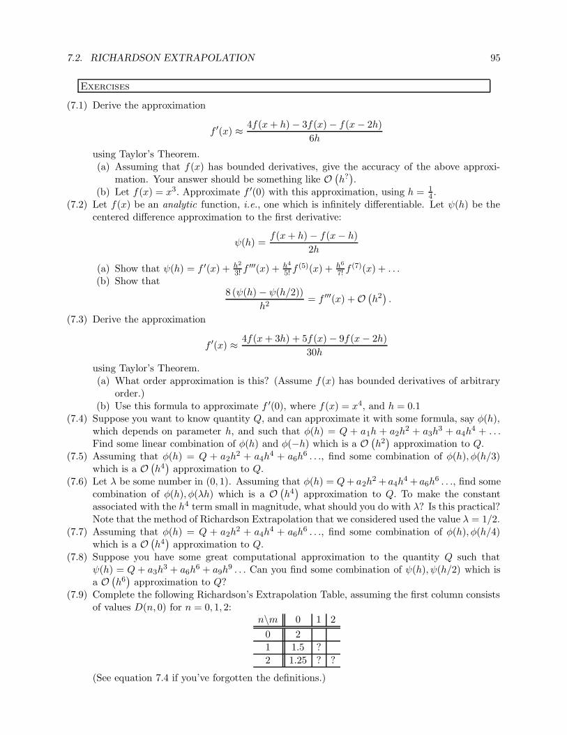
7.2. RICHARDSON EXTRAPOLATION 95
Exercises
(7.1) Derive the approximation
f ′(x) ≈ 4f(x+ h)− 3f(x)− f(x− 2h)
6h
using Taylor’s Theorem.(a) Assuming that f(x) has bounded derivatives, give the accuracy of the above approxi-
mation. Your answer should be something like O(
h?)
.(b) Let f(x) = x3. Approximate f ′(0) with this approximation, using h = 1
4 .(7.2) Let f(x) be an analytic function, i.e., one which is infinitely differentiable. Let ψ(h) be the
centered difference approximation to the first derivative:
ψ(h) =f(x+ h)− f(x− h)
2h
(a) Show that ψ(h) = f ′(x) + h2
3! f′′′(x) + h4
5! f(5)(x) + h6
7! f(7)(x) + . . .
(b) Show that8 (ψ(h)− ψ(h/2))
h2= f ′′′(x) +O
(
h2)
.
(7.3) Derive the approximation
f ′(x) ≈ 4f(x+ 3h) + 5f(x)− 9f(x− 2h)
30h
using Taylor’s Theorem.(a) What order approximation is this? (Assume f(x) has bounded derivatives of arbitrary
order.)(b) Use this formula to approximate f ′(0), where f(x) = x4, and h = 0.1
(7.4) Suppose you want to know quantity Q, and can approximate it with some formula, say φ(h),which depends on parameter h, and such that φ(h) = Q + a1h + a2h
2 + a3h3 + a4h
4 + . . .Find some linear combination of φ(h) and φ(−h) which is a O
(
h2)
approximation to Q.(7.5) Assuming that φ(h) = Q + a2h
2 + a4h4 + a6h
6 . . ., find some combination of φ(h), φ(h/3)which is a O
(
h4)
approximation to Q.(7.6) Let λ be some number in (0, 1). Assuming that φ(h) = Q+ a2h
2 + a4h4 + a6h
6 . . ., find somecombination of φ(h), φ(λh) which is a O
(
h4)
approximation to Q. To make the constantassociated with the h4 term small in magnitude, what should you do with λ? Is this practical?Note that the method of Richardson Extrapolation that we considered used the value λ = 1/2.
(7.7) Assuming that φ(h) = Q + a2h2 + a4h
4 + a6h6 . . ., find some combination of φ(h), φ(h/4)
which is a O(
h4)
approximation to Q.(7.8) Suppose you have some great computational approximation to the quantity Q such that
ψ(h) = Q+ a3h3 + a6h
6 + a9h9 . . . Can you find some combination of ψ(h), ψ(h/2) which is
a O(
h6)
approximation to Q?(7.9) Complete the following Richardson’s Extrapolation Table, assuming the first column consists
of values D(n, 0) for n = 0, 1, 2:n\m 0 1 2
0 2
1 1.5 ?
2 1.25 ? ?
(See equation 7.4 if you’ve forgotten the definitions.)

96 CHAPTER 7. APPROXIMATING DERIVATIVES
(7.10) Write code to complete a Richardson’s Method table, given the first column. Your m-fileshould have header line like:function Dnn = richardsons(col0)
where Dnn is the value at the lower left corner of the table, D(n, n) while col0 is the columnof n+ 1 values D(i, 0), for i = 0, 1, . . . , n. Test your code on the following input:octave:1> col0 = [1 0.5 0.25 0.125 0.0625 0.03125];
octave:2> richardsons(col0)
ans = 0.019042
(a) What do you get when you try the following?octave:5> col0 = [1.5 0.5 1.5 0.5 1.5 0.5 1.5];
octave:6> richardsons(col0)
(b) What do you get when you try the following?octave:7> col0 = [0.9 0.99 0.999 0.9999 0.99999];
octave:8> richardsons(col0)

Chapter 8
Integrals and Quadrature
8.1 The Definite Integral
Often enough the numerical analyst is presented with the challenge of finding the definite integralof some function:
∫ b
af(x) dx.
In your golden years of Calculus, you learned the Fundamental Theorem of Calculus, which claimsthat if f(x) is continuous, and F (x) is an antiderivative of f(x), then
∫ b
af(x) dx = F (b)− F (a).
What you might not have been told in Calculus is there are some functions for which a closedform antiderivative does not exist or at least is not known to humankind. Nevertheless, you mayfind yourself in a situation where you have to evaluate an integral for just such an integrand. Anapproximation will have to do.
8.1.1 Upper and Lower Sums
We will review the definition of the Riemann integral of a function. A partition of an interval [a, b]is a finite, ordered collection of nodes xi:
a = x0 < x1 < x2 < · · · < xn = b.
Given such a partition, P, define the upper and lower bounds on each subinterval [xj , xj+1] asfollows:
mi = inf {f(x) | xi ≤ x ≤ xi+1 }Mi = sup {f(x) | xi ≤ x ≤ xi+1 }
Then for this function f and partition P, define the upper and lower sums:
L(f, P ) =
n−1∑
i=0
mi (xi+1 − xi)
U(f, P ) =n−1∑
i=0
Mi (xi+1 − xi)
97

98 CHAPTER 8. INTEGRALS AND QUADRATURE
We can interpret the upper and lower sums graphically as the sums of areas of rectangles definedby the function f and the partition P , as in Figure 8.1.
bottomright
� � � � � � � � � � � �
(a) The Lower Sumbottomright
� � � � � � � � � � � �
(b) The Upper Sum
Figure 8.1: The (a) lower, and (b) upper sums of a function on a given interval are shown. Theseapproximations to the integral are the sums of areas of rectangles. Note that the lower sums arean underestimate, and the upper sums an overestimate of the integral.
Notice a few things about the upper, lower sums:(i) L(f, P ) ≤ U(f, P ).(ii) If we switch to a “better” partition (i.e., a finer one), we expect that L(f, ·) increases and
U(f, ·) decreases.The notion of integrability familiar from Calculus class (that is Riemann Integrability) is defined
in terms of the upper and lower sums.
Definition 8.1. A function f is Riemann Integrable over interval [a, b] if
supPL(f, P ) = inf
PU(f, P ),
where the supremum and infimum are over all partitions of the interval [a, b]. Moreover, in casef(x) is integrable, we define the integral
∫ b
af(x) dx = inf
PU(f, P ),
You may recall the following
Theorem 8.2. Every continuous function on a closed bounded interval of the real line is RiemannIntegrable (on that interval).
Continuity is sufficient, but not necessary.
Example 8.3. Consider the Heaviside function:
f(x) =
{
0 x < 01 0 ≤ x
This function is not continuous on any interval containing 0, but is Riemann Integrable on everyclosed bounded interval.

8.1. THE DEFINITE INTEGRAL 99
Example 8.4. Consider the Dirichlet function:
f(x) =
{
0 x rational1 x irrational
For any partition P of any interval [a, b], we have L(f, P ) = 0, while U(f, P ) = 1, so
supPL(f, P ) = 0 6= 1 = inf
PU(f, P ),
so this function is not Riemann Integrable.
8.1.2 Approximating the Integral
The definition of the integral gives a simple method of approximating an integral∫ ba f(x) dx. The
method cuts the interval [a, b] into a partition of n equal subintervals xi = a+ b−an , for i = 0, 1, . . . , n.
The algorithm then has to somehow find the supremum and infimum of f(x) on each interval[xi, xi+1]. The integral is then approximated by the mean of the lower and upper sums:
∫ b
af(x) dx ≈ 1
2(L(f, P ) + U(f, P )) .
Because the value of the integral is between L(f, P ) and U(f, P ), this approximation has error atmost
1
2(U(f, P )− L(f, P )) .
Note that in general, or for a black box function, it is usually not feasible to find the supremaand infima of f(x) on the subintervals, and thus the lower and upper sums cannot be calculated.However, if some information is known about the function, it becomes easier:
Example 8.5. Consider for example, using this method on some function f(x) which is monotone
increasing, that is x ≤ y implies f(x) ≤ f(y). In this case, the infimum of f(x) on each intervaloccurs at the leftmost endpoint, while the supremum occurs at the right hand endpoint. Thus forthis partition, P, we have
L(f, P ) =
n−1∑
k=0
mi |xk+1 − xk| =|b− a|n
n−1∑
k=0
f(xk)
U(f, P ) =
n−1∑
k=0
Mi |xk+1 − xk| =|b− a|n
n−1∑
k=0
f(xk+1) =|b− a|n
n∑
k=1
f(xk)
Then the error of the approximation is
1
2(U(f, P )− L(f, P )) =
1
2
|b− a|n
[f(xn)− f(x0)] =|b− a| [f(b)− f(a)]
2n.
8.1.3 Simple and Composite Rules
For the remainder of this chapter we will study “simple” quadrature rules, i.e., rules which approx-imate the integral of a function, f(x) over an interval [a, b] by means of a number of evaluations off at points in this interval. The error of a simple quadrature rule usually depends on the function

100 CHAPTER 8. INTEGRALS AND QUADRATURE
f, and the width of the interval [a, b] to some power which is determined by the rule. That is weusually think of a simple rule as being applied to a small interval.
To use a simple rule on a larger interval, we usually cast it into a “composite” rule. Thus thetrapezoidal rule, which we will study next becomes the composite trapezoidal rule. The means ofextending a simple rule to a composite rule is straightforward: Partition the given interval intosubintervals, apply the simple rule to each subinterval, and sum the results. Thus, for example ifthe interval in question is [α, β], and the partition is α = x0 < x1 < x2 < . . . < xn = β, we have
composite rule on [α, β] =n−1∑
i=0
simple rule applied to [xi, xi+1].
8.2 Trapezoidal Rule
Suppose we are trying to approximate the integral
∫ b
af(x) dx,
for some unpleasant or black box function f(x).The trapezoidal rule approximates the integral
∫ b
af(x) dx
by the (signed) area of the trapezoid through the points (a, f(a)) , (b, f(b)) , and with one side thesegment from a to b. See Figure 8.2.
lleft
uright
PSfrag
replacem
ents
a b
Figure 8.2: The trapezoidal rule for approximating the integral of a function over [a, b] is shown.
By old school math, we can find this signed area easily. This gives the (simple) trapezoidal rule:
∫ b
af(x) dx ≈ (b− a) f(a) + f(b)
2.

8.2. TRAPEZOIDAL RULE 101
The composite trapezoidal rule can be written in a simplified form, one which you saw in yourcalculus class, if the interval in question is partitioned into equal width subintervals. That is if youlet [α, β] be partitioned by
α = x0 < x1 < x2 < x3 < . . . < xn = β,
with xi = α+ ih, where h = (β − α)/n, then the composite trapezoidal rule is
∫ β
αf(x) dx =
n−1∑
i=0
∫ xi+1
xi
f(x) dx ≈ 1
2
n−1∑
i=0
(xi+1 − xi) [f(xi) + f(xi+1)] . (8.1)
Since each subinterval has equal width, xi+1 − xi = h, and we have
∫ b
af(x) dx ≈ h
2
n−1∑
i=0
[f(xi) + f(xi+1)] . (8.2)
In your calculus class, you saw this in the less comprehensible form:
∫ b
af(x) dx ≈ h
[
f(a) + f(b)
2+
n−1∑
i=1
f(xi)
]
.
Note that the composite trapezoidal rule for equal subintervals is the same as the approximationwe found for increasing functions in Example 8.5.
Example Problem 8.6. Approximate the integral
∫ 2
0
1
1 + x2dx
by the composite trapezoidal rule with a partition of equally spaced points, for n = 2.Solution: We have h = 2−0
2 = 1, and f(x0) = 1, f(x1) = 12 , f(x2) = 1
5 . Then the compositetrapezoidal rule gives the value
1
2[f(x0) + f(x1) + f(x1) + f(x2)] =
1
2
[
1 + 1 +1
5
]
=11
10.
The actual value is arctan 2 ≈ 1.107149, and our approximation is correct to two decimal places. a
8.2.1 How Good is the Composite Trapezoidal Rule?
We consider the composite trapezoidal rule for partitions of equal subintervals. Let pi(x) be thepolynomial of degree ≤ 1 that interpolates f(x) at xi, xi+1. Let
Ii =
∫ xi+1
xi
f(x) dx, Ti =
∫ xi+1
xi
pi(x) dx = (xi+1 − xi)pi(xi) + pi(xi+1)
2=h
2(f(xi) + f(xi+1)) .
That’s right: the composite trapezoidal rule approximates the integral of f(x) over [xi, xi+1] bythe integral of pi(x) over the same interval.
Now recall our theorem on polynomial interpolation error. For x ∈ [xi, xi+1] , we have
f(x)− pi(x) =1
(2)!f (2)(ξx) (x− xi) (x− xi+1) ,

102 CHAPTER 8. INTEGRALS AND QUADRATURE
for some ξx ∈ [xi, xi+1] . Recall that ξx depends on x. To make things simpler, call it ξ(x).Now integrate:
Ii − Ti =
∫ xi+1
xi
f(x)− pi(x) dx =1
2
∫ xi+1
xi
f ′′(ξ(x)) (x− xi) (x− xi+1) dx.
We will now attack the integral on the right hand side. Recall the following theorem:
Theorem 8.7 (Mean Value Theorem for Integrals). Suppose f is continuous, g is RiemannIntegrable and does not change sign on [α, β]. Then there is some ζ ∈ [α, β] such that
∫ β
αf(x)g(x) dx = f(ζ)
∫ β
αg(x) dx.
We use this theorem on our integral. Note that (x− xi) (x− xi+1) is nonpositive on the intervalof question, [xi, xi+1]. We assume continuity of f ′′(x), and wave our hands to get continuity off ′′(ξ(x)). Then we have
Ii − Ti =1
2f ′′(ξ)
∫ xi+1
xi
(x− xi) (x− xi+1) dx,
for some ξi ∈ [xi, xi+1]. By boring calculus and algebra, we find that
∫ xi+1
xi
(x− xi) (x− xi+1) dx = −h3
6.
This gives
Ii − Ti = −h3
12f ′′(ξi),
for some ξi ∈ [xi, xi+1].We now sum over all subintervals to find the total error of the composite trapezoidal rule
E =
n−1∑
i=0
Ii − Ti = −h3
12
n−1∑
i=0
f ′′(ξi) = −(b− a) h2
12
[
1
n
n−1∑
i=0
f ′′(ξi)
]
.
On the far right we have an average value, 1n
∑n−1i=0 f
′′(ξi), which lies between the least and greatestvalues of f ′′ on the inteval [a, b], and thus by the IVT, there is some ξ which takes this value. So
E = −(b− a) h2
12f ′′(ξ)
This gives us the theorem:
Theorem 8.8 (Error of the Composite Trapezoidal Rule). Let f ′′(x) be continuous on [a, b].Let T be the value of the trapezoidal rule applied to f(x) on this interval with a partition of uniform
spacing, h, and let I =∫ ba f(x) dx. Then there is some ξ ∈ [a, b] such that
I − T = −(b− a) h2
12f ′′(ξ).
Note that this theorem tells us not only the magnitude of the error, but the sign as well. Thusif, for example, f(x) is concave up and thus f ′′ is positive, then I − T will be negative, i.e., thetrapezoidal rule gives an overestimate of the integral I. See Figure 8.3.

8.2. TRAPEZOIDAL RULE 103
lleft
uright
PSfrag
replacem
ents
xi xi+1
Figure 8.3: The trapezoidal rule is an overestimate for a function which is concave up, i.e., haspositive second derivative.
8.2.2 Using the Error Bound
Example Problem 8.9. How many intervals are required to approximate the integral
ln 2 = I =
∫ 1
0
1
1 + xdx
to within 1× 10⁻¹⁰?Solution: We have f(x) = 1
1+x , thus f ′(x) = − 1(1+x)2 . And f ′′(x) = 2
(1+x)3 . Thus f ′′(ξ) is
continuous and bounded by 2 on [0, 1]. If we use n equal subintervals then Theorem 8.8 tells us theerror will be
−1− 0
12
(
1− 0
n
)2
f ′′(ξ) = −f′′(ξ)
12n2.
To make this smaller than 1× 10⁻¹⁰, in absolute value, we need only take
1
6n2≤ 1× 10⁻¹⁰,
and so n ≥√
16 × 105 suffices. Because f ′′(x) is positive on this interval, the trapezoidal rule will
be an overestimate. aExample Problem 8.10. How many intervals are required to approximate the integral
∫ 2
0x3 − 1 dx
to within 1× 10⁻⁶?Solution: We have f(x) = x3 − 1, thus f ′(x) = 3x2, and f ′′(x) = 6x. Thus f ′′(ξ) is continuousand bounded by 12 on [0, 2]. If we use n equal subintervals then by Theorem 8.8 the error will be
−2− 0
12
(
2− 0
n
)2
f ′′(ξ) = −2f ′′(ξ)
3n2.

104 CHAPTER 8. INTEGRALS AND QUADRATURE
To make this smaller than 1× 10⁻⁶, in absolute value, it suffices to take
24
3n2≤ 1× 10⁻⁶,
and so n ≥√
8 × 10³ suffices. Because f ′′(x) is positive on this interval, the trapezoidal rule willbe an overestimate. a
8.3 Romberg Algorithm
Theorem 8.8 tells us, approximately, that the error of the composite trapezoidal rule approximationis O
(
h2)
. If we halve h, the error is quartered. Sometimes we want to do better than this. We’lluse the same trick that we did from Richardson extrapolation. In fact, the forms are exactly thesame.
Towards this end, suppose that f, a, b are given. For a given n, we are going to use the trapezoidalrule on a partition of 2n equal subintervals of [a, b]. That is h = b−a
2n . Then define
φ(n) =1
2
b− a2n
2n−1∑
i=0
f(xi) + f(xi+1)
=b− a2n
[
f(a)
2+f(b)
2+
2n−1∑
i=1
f
(
a+ ib− a2n
)
]
.
The intervals used to calculate φ(n + 1) are half the size of those for φ(n). As mentioned above,this means the error is one quarter.
It turns out that if we had proved the error theorem differently, we would have proved therelation:
φ(n) =
∫ b
af(x) dx+ a2h
2n + a4h
4n + a6h
6n + a8h
8n + . . . ,
where hn = b−a2n . The constants ai are a function of f (i)(x) only. This should look just like something
from Chapter 7. What happens if we now calculate φ(n+ 1)? We have
φ(n+ 1) =
∫ b
af(x) dx+ a2h
2n+1 + a4h
4n+1 + a6h
6n+1 + a8h
8n+1 + . . . ,
=
∫ b
af(x) dx+
1
4a2h
2n +
1
16a4h
4n +
1
64a6h
6n +
1
256a8h
8n + . . . .
This happens because hn+1 = b−a2n+1 = 1
2b−a2n = hn
2 . As with Richardon’s method for approximatingderivatives, we now combine the right multiples of these:
φ(n)− 4φ(n+ 1) = −3
∫ b
af(x) dx+
3
44h4
n +15
16a6h
6n +
63
64a8h
8n + . . .
4φ(n)− φ(n+ 1)
3=
∫ b
af(x) dx− 1
44h4
n −5
16a6h
6n −
21
64a8h
8n + . . .
This approximation has a truncation error of O(
h4n
)
.Like in Richardson’s method, we can use this to get better and better approximations to the
integral. We do this by constructing a triangular array of approximations, each entry dependingon two others. Towards this end, we let
R(n, 0) = φ(n),
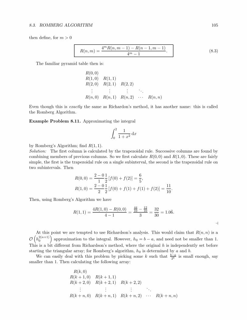
8.3. ROMBERG ALGORITHM 105
then define, for m > 0
R(n,m) =4mR(n,m− 1)−R(n− 1,m− 1)
4m − 1. (8.3)
The familiar pyramid table then is:
R(0, 0)R(1, 0) R(1, 1)R(2, 0) R(2, 1) R(2, 2)
......
.... . .
R(n, 0) R(n, 1) R(n, 2) · · · R(n, n)
Even though this is exactly the same as Richardon’s method, it has another name: this is calledthe Romberg Algorithm.
Example Problem 8.11. Approximating the integral
∫ 2
0
1
1 + x2dx
by Romberg’s Algorithm; find R(1, 1).Solution: The first column is calculated by the trapezoidal rule. Successive columns are found bycombining members of previous columns. So we first calculate R(0, 0) and R(1, 0). These are fairlysimple, the first is the trapezoidal rule on a single subinterval, the second is the trapezoidal rule ontwo subintervals. Then
R(0, 0) =2− 0
1
1
2[f(0) + f(2)] =
6
5,
R(1, 0) =2− 0
2
1
2[f(0) + f(1) + f(1) + f(2)] =
11
10.
Then, using Romberg’s Algorithm we have
R(1, 1) =4R(1, 0) −R(0, 0)
4− 1=
4410 − 12
10
3=
32
30= 1.06.
a
At this point we are tempted to use Richardson’s analysis. This would claim that R(n, n) is a
O(
h2(n+1)0
)
approximation to the integral. However, h0 = b− a, and need not be smaller than 1.
This is a bit different from Richardson’s method, where the original h is independently set beforestarting the triangular array; for Romberg’s algorithm, h0 is determined by a and b.
We can easily deal with this problem by picking some k such that b−a2k is small enough, say
smaller than 1. Then calculating the following array:
R(k, 0)R(k + 1, 0) R(k + 1, 1)R(k + 2, 0) R(k + 2, 1) R(k + 2, 2)
......
.... . .
R(k + n, 0) R(k + n, 1) R(k + n, 2) · · · R(k + n, n)

106 CHAPTER 8. INTEGRALS AND QUADRATURE
Quite often Romberg’s Algorithm is used to compute columns of this array. Subtractive can-celling or unbounded higher derivatives of f(x) can make successive approximations less accurate.For this reason, entries in ever rightward columns are usually not calculated, rather lower entriesin a single column are calculated instead. That is, the user calculates the array:
R(k, 0)R(k + 1, 0) R(k + 1, 1)R(k + 2, 0) R(k + 2, 1) R(k + 2, 2)
......
.... . .
R(k + n, 0) R(k + n, 1) R(k + n, 2) · · · R(k + n, n)R(k + n+ 1, 0) R(k + n+ 1, 1) R(k + n+ 1, 2) · · · R(k + n+ 1, n)R(k + n+ 2, 0) R(k + n+ 2, 1) R(k + n+ 2, 2) · · · R(k + n+ 2, n)R(k + n+ 3, 0) R(k + n+ 3, 1) R(k + n+ 3, 2) · · · R(k + n+ 3, n)
......
......
Then R(k + n+ l, n) makes a fine approximation to the integral as l →∞. Usually n is small,like 2 or 3.
8.3.1 Recursive Trapezoidal Rule
It turns out there is an efficient way of calculating R(n+ 1, 0) given R(n, 0); first notice from theabove example that
R(0, 0) =b− a
1
1
2[f(a) + f(b)] ,
R(1, 0) =b− a
2
1
2
[
f(a) + f(a+ b
2) + f(
a+ b
2) + f(b)
]
.
It would be best to calculate R(1, 0) without recalculating f(a) and f(b). It turns out this is possible.Let hn = b−a
2n , and recall that
R(n, 0) = φ(n) = hn
[
f(a) + f(b)
2+
2n−1∑
i=1
f (a+ ihn)
]
.
Thus
R(n+ 1, 0) = φ(n+ 1) = hn+1
f(a) + f(b)
2+
2n+1−1∑
i=1
f (a+ ihn+1)
,
=1
2hn
[
f(a) + f(b)
2+
2n−1∑
i=1
f (a+ (2i − 1)hn+1) + f
(
a+ (2i)1
2hn
)
]
,
=1
2hn
[
f(a) + f(b)
2+
2n−1∑
i=1
f (a+ ihn) +2n−1∑
i=1
f (a+ (2i− 1)hn+1)
]
,
=1
2R(n, 0) + hn+1
2n−1∑
i=1
f (a+ (2i − 1)hn+1) .
Then calculating R(n+ 1, 0) requires only 2n − 1 additional evaluations of f(x), instead of the2n+1 + 1 usually required.

8.4. GAUSSIAN QUADRATURE 107
8.4 Gaussian Quadrature
The word quadrature refers to a method of approximating the integral of a function as the linearcombination of the function at certain points, i.e.,
∫ b
af(x) dx ≈ A0f(x0) +A1f(x1) + . . . Anf(xn), (8.4)
for some collection of nodes {xi}ni=0, and weights {Ai}ni=0. Normally one finds the nodes and weightsin a table somewhere; we expect a quadrature rule with more nodes to be more accurate in somesense–the tradeoff is in the number of evaluations of f(·). We will examine how these rules arecreated.
8.4.1 Determining Weights (Lagrange Polynomial Method)
Suppose that the nodes {xi}ni=0 are given. An easy way to find “good” weights {Ai}ni=0 for thesenodes is to rig them so the quadrature rule gives the integral of p(x), the polynomial of degree ≤ nwhich interpolates f(x) on these nodes. Recall
p(x) =n∑
i=0
f(xi)`i(x),
where `i(x) is the ith Lagrange polynomial. Thus our rigged approximation is the one that gives∫ b
af(x) dx ≈
∫ b
ap(x) dx =
n∑
i=0
f(xi)
∫ b
a`i(x) dx.
If we let
Ai =
∫ b
a`i(x) dx,
then we have a quadrature rule.If f(x) is a polynomial of degree ≤ n then f(x) = p(x), and the quadrature rule is exact.
Example Problem 8.12. Construct a quadrature rule on the interval [0, 4] using nodes 0, 1, 2.Solution: The nodes are given, we determine the weights by constructing the Lagrange Polyno-mials, and integrating them.
`0(x) =(x− 1)(x− 2)
(0− 1)(0− 2)=
1
2(x− 1)(x− 2),
`1(x) =(x− 0)(x− 2)
(1− 0)(1− 2)= −(x)(x− 2),
`2(x) =(x− 0)(x− 1)
(2− 0)(2− 1)=
1
2(x)(x− 1).
Then the weights are
A0 =
∫ 4
0`0(x) dx =
∫ 4
0
1
2(x− 1)(x − 2) dx =
8
3,
A1 =
∫ 4
0`1(x) dx =
∫ 4
0−(x)(x− 2) dx = −16
3,
A2 =
∫ 4
0`2(x) dx =
∫ 4
0
1
2(x)(x− 1) dx =
20
3.

108 CHAPTER 8. INTEGRALS AND QUADRATURE
Thus our quadrature rule is
∫ 4
0f(x) dx ≈ 8
3f(0)− 16
3f(1) +
20
3f(2).
We expect this rule to be exact for a quadratic function f(x). To illustrate this, let f(x) = x2+1.By calculus we have
∫ 4
0x2 + 1 dx =
1
3x3 + x
∣
∣
∣
∣
4
0
=64
3+ 4 =
76
3.
The approximation is∫ 4
0x2 + 1 dx ≈ 8
3[0 + 1]− 16
3[1 + 1] +
20
3[4 + 1] =
76
3.
a
8.4.2 Determining Weights (Method of Undetermined Coefficients)
Using the Lagrange Polynomial Method to find the weights Ai is fine for a computer, but canbe tedious (and error-prone) if done by hand (say, on an exam). The method of undeterminedcoefficients is a good alternative for finding the weights by hand, and for small n.
The idea behind the method is to find n+1 equations involving the n+1 weights. The equationsare derived by letting the quadrature rule be exact for f(x) = xj for j = 0, 1, . . . , n. That is, setting
∫ b
axj dx =
n∑
i=0
Ai(xi)j .
For example, we reconsider Example Problem 8.12.
Example Problem 8.13. Construct a quadrature rule on the interval [0, 4] using nodes 0, 1, 2.Solution: The method of undetermined coefficients gives the equations:
∫ 4
01 dx = 4 = A0 +A1 +A2
∫ 4
0xdx = 8 = A1 + 2A2
∫ 4
0x2 dx = 64/3 = A1 + 4A2.
We perform Naıve Gaussian Elimination on the system:
1 1 1 40 1 2 80 1 4 64/3
We get the same weights as in Example Problem 8.12: A2 = 203 , A1 = −16
3 , A0 = 83 . a
Notice the difference compared to the Lagrange Polynomial Method: undetermined coefficientsrequires solution of a linear system, while the former method calculates the weights “directly.”Since we will not consider n to be very large, solving the linear system may not be too burdensome.
Moreover, the method of undetermined coefficients is useful in more general settings, as illus-trated by the next example:

8.4. GAUSSIAN QUADRATURE 109
Example Problem 8.14. Determine a “quadrature” rule of the form
∫ 1
0f(x) dx ≈ Af(1) +Bf ′(1) + Cf ′′(1)
that is exact for polynomials of highest possible degree. What is the highest degree polynomial forwhich this rule is exact?Solution: Since there are three unknown coefficients to be determined, we look for three equations.We get these equations by plugging in successive polynomials. That is, we plug in f(x) = 1, x, x2
and assuming the coefficients give equality:
∫ 1
01 dx = 1 = A 1 +B 0 +C 0 = A
∫ 1
0xdx = 1/2 = A 1 +B 1 +C 0 = A+B
∫ 1
0x2 dx = 1/3 = A 1 +B 2 +C 2 = A+ 2B + 2C
This is solved by A = 1, B = −1/2, C = 1/6. This rule should be exact for polynomials of degreeno greater than 2, but it might be better. We should check:
∫ 1
0x3 dx = 1/4 6= 1/2 = 1− 3/2 + 1 = A 1 +B 3 + C 6,
and thus the rule is not exact for cubic polynomials, or those of higher degree. a
8.4.3 Gaussian Nodes
It would seem this is the best we can do: using n+1 nodes we can devise a quadrature rule that isexact for polynomials of degree ≤ n by choosing the weights correctly. It turns out that by choosingthe nodes in the right way, we can do far better. Gauss discovered that the right nodes to chooseare the n+ 1 roots of the (nontrivial) polynomial, q(x), of degree n+ 1 which has the property
∫ b
axkq(x) dx = 0 (0 ≤ k ≤ n) .
(If you view the integral as an inner product, you could say that q(x) is orthogonal to the polyno-mials xk in the resultant inner product space, but that’s just fancy talk.)
Suppose that we have such a q(x)–we will not prove existence or uniqueness. Let f(x) be apolynomial of degree ≤ 2n+ 1. We write
f(x) = p(x)q(x) + r(x).
Both p(x), r(x) are of degree ≤ n. Because of how we picked q(x) we have
∫ b
ap(x)q(x) dx = 0.
Thus∫ b
af(x) dx =
∫ b
ap(x)q(x) dx+
∫ b
ar(x)dx =
∫ b
ar(x)dx.
110 CHAPTER 8. INTEGRALS AND QUADRATURE
Now suppose that the Ai are chosen by Lagrange Polynomials so the quadrature rule on thenodes xi is exact for polynomials of degree ≤ n. Then
n∑
i=0
Aif(xi) =n∑
i=0
Ai [p(xi)q(xi) + r(xi)] =n∑
i=0
Air(xi).
The last equality holds because the xi are the roots of q(x). Because of how the Ai are chosen wethen have
n∑
i=0
Aif(xi) =
n∑
i=0
Air(xi) =
∫ b
ar(x) dx =
∫ b
af(x) dx.
Thus this rule is exact for f(x). We have (or rather, Gauss has) made quadrature twice as good.
Theorem 8.15 (Gaussian Quadrature Theorem). Let xi be the n+ 1 roots of a (nontrivial)polynomial, q(x), of degree n+ 1 which has the property
∫ b
axkq(x) dx = 0 (0 ≤ k ≤ n) .
Let Ai be the coefficients for these nodes chosen by integrating the Lagrange Polynomials. Then thequadrature rule for this choice of nodes and coefficients is exact for polynomials of degree ≤ 2n+1.
8.4.4 Determining Gaussian Nodes
We can determine the Gaussian nodes in the same way we determine coefficients. The example isillustrative
Example Problem 8.16. Find the two Gaussian nodes for a quadrature rule on the interval [0, 2].Solution: We will find the function q(x) of degree 2, which is “orthogonal” to 1, x under the innerproduct of integration over [0, 2]. Thus we let q(x) = c0 + c1x+ c2x
2. The orthogonality conditionbecomes
∫ 2
01q(x) dx =
∫ 2
0xq(x) dx = 0 that is,
∫ 2
0c0 + c1x+ c2x
2 dx =
∫ 2
0c0x+ c1x
2 + c2x3 dx = 0
Evaluating these integrals gives the following system of linear equations:
2c0 + 2c1 +8
3c2 = 0,
2c0 +8
3c1 + 4c2 = 0.
This system is “underdetermined,” that is, there are two equations, but three unknowns. Notice,however, that if q(x) satisfies the orthogonality conditions, then so does q(x) = αq(x), for any realnumber α. That is, we can pick the scaling of q(x) as we wish.
With great foresight, we “guess” that we want c2 = 3. This reduces the equations to
2c0 + 2c1 = −8,
2c0 +8
3c1 = −12.

8.4. GAUSSIAN QUADRATURE 111
Simple Gaussian Elimination (cf. Chapter 3) yields the answer c0 = 2, c1 = −6, c2 = 3.Then our nodes are the roots of q(x) = 2− 6x+ 3x2. That is the roots
6±√
36− 24
6= 1±
√3
3.
These nodes are a bit ugly. Rather than construct the Lagrange Polynomials, we will use themethod of undetermined coefficients. Remember, we want to construct A0, A1 such that
∫ 2
0f(x) dx ≈ A0f(1−
√3
3) +A1f(1 +
√3
3)
is exact for polynomial f(x) of degree ≤ 1. It suffices to make this approximation exact for the“building blocks” of such polynomials, that is, for the functions 1 and x. That is, it suffices to findA0, A1 such that
∫ 2
01 dx = A0 +A1
∫ 2
0xdx = A0(1−
√3
3) +A1(1 +
√3
3)
This gives the equations
2 = A0 +A1
2 = A0(1−√
3
3) +A1(1 +
√3
3)
This is solved by A0 = A1 = 1.Thus our quadrature rule is
∫ 2
0f(x) dx ≈ f(1−
√3
3) + f(1 +
√3
3) .
We expect this rule to be exact for cubic polynomials. a
Example Problem 8.17. Verify the results of the previous example problem for f(x) = x3.Solution: We have
∫ 2
0f(x) dx = (1/4) x4
∣
∣
∣
2
0= 4.
The quadrature rule gives
f(1−√
3
3) + f(1 +
√3
3) =
(
1−√
3
3
)3
+
(
1 +
√3
3
)3
=
(
1− 3
√3
3+ 3
3
9− 3√
3
27
)
+
(
1 + 3
√3
3+ 3
3
9+
3√
3
27
)
=(
2−√
3−√
3/9)
+(
2 +√
3 +√
3/9)
= 4
Thus the quadrature rule is exact for f(x). a

112 CHAPTER 8. INTEGRALS AND QUADRATURE
8.4.5 Reinventing the Wheel
While it is good to know the theory, it doesn’t make sense in practice to recompute these things allthe time. There are books full of quadrature rules; any good textbook will list a few. The simplestones are given in Table 8.1.See also http://mathworld.wolfram.com/Legendre-GaussQuadrature.html
n xi Ai
0 x0 = 0 A0 = 2
1x0 = −
√
1/3 A0 = 1
x1 =√
1/3 A1 = 1
x0 = −√
3/5 A0 = 5/92 x1 = 0 A1 = 8/9
x2 =√
3/5 A1 = 5/9
Table 8.1: Gaussian Quadrature rules for the interval [−1, 1]. Thus∫ 1−1 f(x) dx ≈
∑ni=0Aif(xi),
with this relation holding exactly for all polynomials of degree no greater than 2n+ 1.
Quadrature rules are normally given for the interval [−1, 1]. On first consideration, it wouldseem you need a different rule for each interval [a, b]. This is not the case, as the following exampleproblem illustrates:
Example Problem 8.18. Given a quadrature rule which is good on the interval [−1, 1], derive aversion of the rule to apply to the interval [a, b].Solution: Consider the substitution:
x =b− a
2t+
b+ a
2, so dx =
b− a2
dt.
Then∫ b
af(x) dx =
∫ 1
−1f
(
b− a2
t+b+ a
2
)
b− a2
dt.
Letting
g(t) =b− a
2f
(
b− a2
t+b+ a
2
)
,
if f(x) is a polynomial, g(t) is a polynomial of the same degree. Thus we can use the quadraturerule for [−1, 1] on g(t) to evaluate the integral of f(x) over [a, b]. aExample Problem 8.19. Derive the quadrature rules of Example Problem 8.16 by using thetechnique of Example Problem 8.18 and the quadrature rules of Table 8.1.Solution: We have a = 0, b = 2. Thus
g(t) =b− a
2f
(
b− a2
t+b+ a
2
)
= f(t+ 1).
To integrate f(x) over [0, 2], we integrate g(t) over [−1, 1]. The standard Gaussian Quadrature ruleapproximates this as
∫ 1
−1g(t) dt ≈ g(−
√
1/3) + g(√
1/3) = f(1−√
1/3) + f(1 +√
1/3).
This is the same rule that was derived (with much more work) in Example Problem 8.16. a

8.4. GAUSSIAN QUADRATURE 113
Exercises
(8.1) Use the composite trapezoidal rule, by hand, to approximate
∫ 3
0x2 dx (= 9)
Use the partition {xi}2i=0 = {0, 1, 3} . Why is your approximation an overestimate?(8.2) Use the composite trapezoidal rule, by hand, to approximate
∫ 1
0
1
x+ 1dx (= ln 2 ≈ 0.693)
Use the partition {xi}3i=0 ={
0, 14 ,
12 , 1}
.Why is your approximation an overestimate? (Check:
I think the answer is 0.7)(8.3) Use the composite trapezoidal rule, by hand to approximate
∫ 1
0
4
1 + x2dx.
Use n = 4 subintervals. How good is your answer?(8.4) Use Theorem 8.8 to bound the error of the composite trapezoidal rule approximation of
∫ 20 x
3 dx with n = 10 intervals. You should find that the approximation is an overestimate.
(8.5) How many equal subintervals of [0, 1] are required to approximate∫ 10 cos x dx with error
smaller than 1× 10⁻⁶ by the composite trapezoidal rule? (Use Theorem 8.8.)(8.6) How many equal subintervals would be required to approximate
∫ 1
0
4
1 + x2dx.
to within 0.0001 by the composite trapezoidal rule? (Hint: Use the fact that |f ′′(x)| ≤ 8 on[0, 1] for f(x) = 4/(1 + x2))
(8.7) How many equal subintervals of [2, 3] are required to approximate∫ 32 e
x dx with error smallerthan 1× 10⁻³ by the composite trapezoidal rule?
(8.8) Simpson’s Rule for quadrature is given as
∫ b
af(x) dx ≈ ∆x
3[f(x0) + 4f(x1) + 2f(x2) + 4f(x3) + . . . + 2f(xn−2) + 4f(xn−1) + f(xn)] ,
where ∆x = (b− a)/n, and n is assumed to be even. Show that Simpson’s Rule for n = 2 isactually given by Romberg’s Algorithm as R(1, 1). As such we expect Simpson’s Rule to bea O
(
h4)
approximation to the integral.(8.9) Find a quadrature rule of the form
∫ 1
0f(x) dx ≈ Af(0) +Bf(1/2) + Cf(1)
that is exact for polynomials of highest possible degree. What is the highest degree polynomialfor which this rule is exact?
114 CHAPTER 8. INTEGRALS AND QUADRATURE
(8.10) Determine a “quadrature” rule of the form
∫ 1
−1f(x) dx ≈ Af(0) +Bf ′(−1) + Cf ′(1)
that is exact for polynomials of highest possible degree. What is the highest degree polynomialfor which this rule is exact? (Since this rule uses derivatives of f, it does not exactly fit ourdefinition of a quadrature rule, but it may be applicable in some situations.)
(8.11) Determine a “quadrature” rule of the form
∫ 1
0f(x) dx ≈ Af(0) +Bf ′(0) + Cf(1)
that is exact for polynomials of highest possible degree. What is the highest degree polynomialfor which this rule is exact?
(8.12) Consider the so-called order n Chebyshev Quadrature rule:
∫ 1
−1f(x) dx ≈ cn
n∑
i=0
f(xi)
Find the weighting cn and nodes xi for the case n = 2 and the case n = 3. For what orderpolynomials are these rules exact?
(8.13) Find the Gaussian Quadrature rule with 2 nodes for the interval [1, 5], i.e., find a rule
∫ 5
1f(x) dx ≈ Af(x0) +Bf(x1)
Before you solve the problem, consider the following questions: do you expect the nodes tobe the endpoints 1 and 5? do you expect the nodes to be arranged symmetrically around themidpoint of the interval?
(8.14) Find the Gaussian Quadrature rule with 3 nodes for the interval [−1, 1], i.e., find a rule
∫ 1
−1f(x) dx ≈ Af(x0) +Bf(x1) +Cf(x2)
To find the nodes x0, x1, x2 you will have to find the zeroes of a cubic equation, which could bedifficult. However, you may use the simplifying assumption that the nodes are symmetricallyplaced in the interval [−1, 1].
(8.15) Write code to approximate the integral of a f on [a, b] by the composite trapezoidal rule onn equal subintervals. Your m-file should have header line like:function iappx = trapezoidal(f,a,b,n)
You may wish to use the code:x = a .+ (b-a) .* (0:n) ./ n;
If f is defined to work on vectors element-wise, you can probably speed up your computationby usingbigsum = 0.5 * ( f(x(1)) + f(x(n+1)) ) + sum( f(x(2:(n))) );
(8.16) Write code to implement the Gaussian Quadrature rule for n = 2 to integrate f on theinterval [a, b]. Your m-file should have header line like:function iappx = gauss2(f,a,b)
(8.17) Write code to implement composite Gaussian Quadrature based on code from the previousproblem. Something like the following probably works:

8.4. GAUSSIAN QUADRATURE 115
function iappx = gaussComp(f,a,b,n)
% code to approximate integral of f over n equal subintervals of [a,b]
x = a .+ (b-a) .* (0:n) ./ n;
iappx = 0;
for i=1:n
iappx += gauss2(f,x(i),x(i+1));
end
Use your code to approximate the error function:
erf(z) =2√π
∫ z
0e−t2 dt.
Compare your results with the octave/Matlab builtin function erf. (Try help erf in octave,or see http://mathworld.wolfram.com/Erf.html)The error function is used in probability. In particular, the probability that a normal randomvariable is within z standard deviations from its mean is
erf(z/√
2)
Thus erf(1/√
2) ≈ 0.683, and erf(2/√
2) ≈ 0.955. These numbers should look familiar to you.

116 CHAPTER 8. INTEGRALS AND QUADRATURE

Chapter 9
Least Squares
9.1 Least Squares
Least squares is a general class of methods for fitting observed data to a theoretical model function.In the general setting we are given a set of data
x x0 x1 . . . xn
y y0 y1 . . . yn
and some class of functions, F . The goal then is to find the “best” f ∈ F to fit the data to y = f(x).Usually the class of functions F will be determined by some small number of parameters; the numberof parameters will be smaller (usually much smaller) than the number of data points. The theoryhere will be concerned with defining “best,” and examining methods for finding the “best” functionto fit the data.
9.1.1 The Definition of Ordinary Least Squares
First we consider the data to be two vectors of length n+ 1. That is we let
x = [x0 x1 . . . xn]> , and y = [y0 y1 . . . yn]> .
The error, or residual, of a given function with respect to this data is the vector r = y − f(x).That is
r = [r0 r1 . . . rn]> , where ri = yi − f(xi).
Our goal is to find f ∈ F such that r is reasonably small. We measure the size of a vectorby the use of norms, which were explored in Subsection 1.4.1. The most useful norms are the `p
norms. For a given p with 0 < p <∞, the `p norm of r is defined as
‖r‖p =
(
n∑
i=0
rpi
)1/p
For the purposes of approximation, the easiest norm to use is the `2 norm:
Definition 9.1.1 ((Ordinary) Least Squares Best Approximant). The least-squares best
approximant to a set of data, x, y from a class of functions, F , is the function f ∗ ∈ F thatminimizes the `2 norm of the error. That is, if f ∗ is the least squares best approximant, then
‖y − f∗(x)‖2 = minf∈F‖y − f(x)‖2
117

118 CHAPTER 9. LEAST SQUARES
We will generally assume uniqueness of the minimum. This method is sometimes called the ordinary
least squares method. It assumes there is no error in the measurement of the data x, and usuallyadmits a relatively straightforward solution.
9.1.2 Linear Least Squares
We illustrate this definition using the class of linear functions as an example, as this case is reason-ably simple. We are assuming
F = {f(x) = ax+ b | a, b ∈ R } .
We can now think of our job as drawing the “best” line through the data.By Definition 9.1.1, we want to find the function f(x) = ax+ b that minimizes
(
n∑
i=0
[yi − f(xi)]2
)1/2
.
This is a minimization problem over two variables, x and y. As you may recall from calculus class,it suffices to minimize the sum rather than its square root. That is, it suffices to minimize
n∑
i=0
[axi + b− yi]2.
We minimize this function with calculus. We set
0 =∂φ
a=
n∑
k=0
2xk (axk + b− yk)
0 =∂φ
b=
n∑
k=0
2 (axk + b− yk)
These are called the normal equations. Believe it or not these are two equations in two unknowns.They can be reduced to
∑
x2ka+
∑
xkb =∑
xkyk∑
xka+ (n+ 1)b =∑
yk
The solution is found by naıve Gaussian Elimination, and is ugly. Let
d11 =∑
x2k
d12 = d21 =∑
xk
d22 = n+ 1
e1 =∑
xkyk
e2 =∑
yk
We want to solve
d11a+ d12b = e1
d21a+ d22b = e2
9.1. LEAST SQUARES 119
Gaussian Elimination produces
a =d22e1 − d12e2d22d11 − d12d21
b =d11e2 − d21e1d22d11 − d12d21
The answer is not so enlightening as the means of finding the solution.
We should, for a moment, consider whether this is indeed the solution. Our calculations haveonly shown an extrema at this choice of (a, b); could it not be a maxima?
9.1.3 Least Squares from Basis Functions
In many, but not all cases, the class of functions, F , is the span of a small set of functions. Thiscase is simpler to explore and we consider it here. In this case F can be viewed as a vector spaceover the real numbers. That is, for f, g ∈ F , and α, β ∈ R, then αf + βg ∈ F , where the functionαf is that function such that (αf)(x) = αf(x).
Now let {gj(x)}mj=0 be a set of m+ 1 linearly independent functions, i.e.,
c0g0(x) + c1g1(x) + . . .+ cmgm(x) = 0 ∀x ⇒ c0 = c1 = . . . = cm = 0
Then we say that F is spanned by the functions {gj(x)}mj=0 if
F =
f(x) =∑
j
cjgj(x) | cj ∈ R, j = 0, 1, . . . ,m
.
In this case the functions gj are basis functions for F . Note the basis functions need not be unique:a given class of functions will usually have more than one choice of basis functions.
Example 9.1. The class F = {f(x) = ax+ b | a, b ∈ R} is spanned by the two functions g0(x) = 1,and g1(x) = x. However, it is also spanned by the two functions g0(x) = 2x+1, and g1(x) = x− 1.
To find the least squares best approximant of F for a given set of data, we minimize the squareof the `2 norm of the error; that is we minimize the function
φ (c0, c1, . . . , cm) =n∑
k=0
∑
j
cjgj(xk)
− yk
2
(9.1)
Again we set partials to zero and solve
0 =∂φ
ci=
n∑
k=0
2
∑
j
cjgj(xk)
− yk
gi(xk)
This can be rearranged to get
m∑
j=0
[
∑
k
gj(xk)gi(xk)
]
cj =n∑
k=0
ykgi(xk)

120 CHAPTER 9. LEAST SQUARES
If we now let
dij =
n∑
k=0
gj(xk)gi(xk), ei =
n∑
k=0
ykgi(xk),
Then we have reduced the problem to the linear system (again, called the normal equations):
d00 d01 d02 · · · d0m
d10 d11 d12 · · · d1m
d20 d21 d22 · · · d2m...
......
. . ....
dm0 dm1 dm2 · · · dmm
c0c1c2...cm
=
e0e1e2...em
(9.2)
The choice of the basis functions can affect how easy it is to solve this system. We explore thisin Section 9.2. Note that we are talking about the basis {gj}mj=0, and not exactly about the classof functions F .
For example, consider what would happen if the system of normal equations were diagonal. Inthis case, solving the system would be rather trivial.
Example Problem 9.2. Consider the case where m = 0, and g0(x) = lnx. Find the least squaresapproximation of the data
x 0.50 0.75 1.0 1.50 2.0 2.25 2.75 3.0
y −1.187098 −0.452472 −0.068077 0.713938 1.165234 1.436975 1.725919 1.841422
Solution: Essentially we are trying to find the c such that c lnx best approximates the data. Thesystem of equation 9.2 reduces to the 1-D equation:
[
Σk ln2 xk
]
c = Σkyk lnxk
For our data, this reduces to:4.0960c = 6.9844
so we find c = 1.7052. The data and the least squares interpolant are shown in Figure 9.1. a
Example 9.3. Consider the awfully chosen basis functions:
g0(x) =( ε
2− 1)
x2 − ε
2x+ 1
g1(x) = x3 +( ε
2− 1)
(
x2 + x)
+ 1
where ε is small, around machine precision.Suppose the data are given at the nodes x0 = 0, x1 = 1, x2 = −1. We want to set up the normal
equations, so we compute some of the dij . First we have to evaluate the basis functions at the nodesxi. But this example was rigged to give:
g0(x0) = 1, g0(x1) = 0, g0(x2) = ε
g1(x0) = 1, g1(x1) = ε, g1(x2) = 0
After much work we find we want to solve[
1 + ε2 11 1 + ε2
] [
c0c1
]
=
[
y0 + εy2
y0 + εy1
]
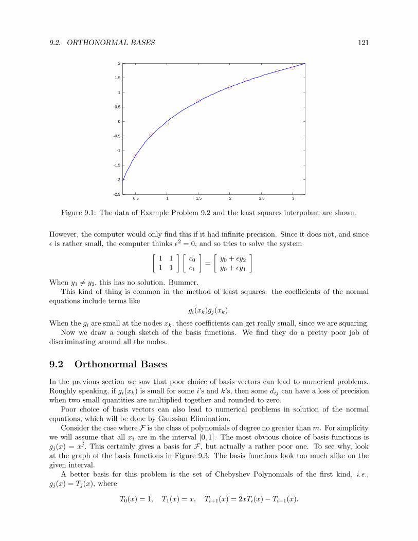
9.2. ORTHONORMAL BASES 121
-2.5
-2
-1.5
-1
-0.5
0
0.5
1
1.5
2
0.5 1 1.5 2 2.5 3
Figure 9.1: The data of Example Problem 9.2 and the least squares interpolant are shown.
However, the computer would only find this if it had infinite precision. Since it does not, and sinceε is rather small, the computer thinks ε2 = 0, and so tries to solve the system
[
1 11 1
] [
c0c1
]
=
[
y0 + εy2
y0 + εy1
]
When y1 6= y2, this has no solution. Bummer.This kind of thing is common in the method of least squares: the coefficients of the normal
equations include terms likegi(xk)gj(xk).
When the gi are small at the nodes xk, these coefficients can get really small, since we are squaring.Now we draw a rough sketch of the basis functions. We find they do a pretty poor job of
discriminating around all the nodes.
9.2 Orthonormal Bases
In the previous section we saw that poor choice of basis vectors can lead to numerical problems.Roughly speaking, if gi(xk) is small for some i’s and k’s, then some dij can have a loss of precisionwhen two small quantities are multiplied together and rounded to zero.
Poor choice of basis vectors can also lead to numerical problems in solution of the normalequations, which will be done by Gaussian Elimination.
Consider the case where F is the class of polynomials of degree no greater thanm. For simplicitywe will assume that all xi are in the interval [0, 1]. The most obvious choice of basis functions isgj(x) = xj. This certainly gives a basis for F , but actually a rather poor one. To see why, lookat the graph of the basis functions in Figure 9.3. The basis functions look too much alike on thegiven interval.
A better basis for this problem is the set of Chebyshev Polynomials of the first kind, i.e.,gj(x) = Tj(x), where
T0(x) = 1, T1(x) = x, Ti+1(x) = 2xTi(x)− Ti−1(x).

122 CHAPTER 9. LEAST SQUARES
-1.5
-1
-0.5
0
0.5
1
1.5
-1 -0.5 0 0.5 1
PSfrag
replacem
ents
g0(x)g1(x)
Figure 9.2: The basis functions g0(x) =(
ε2 − 1
)
x2− ε2x+ 1, and g1(x) = x3 +
(
ε2 − 1
) (
x2 + x)
+ 1are shown for ε = 0.05. Note that around the three nodes 0, 1,−1, these two functions take nearlyidentical values. This can lead to a system of normal equations with no solution.
0
0.2
0.4
0.6
0.8
1
0 0.2 0.4 0.6 0.8 1
PSfrag
replacem
entsx
i
xi+
1
Figure 9.3: The polynomials xi for i = 0, 1, . . . , 6 are shown on [0, 1]. These polynomials make abad basis because they look so much alike, essentially.
These polynomials are illustrated in Figure 9.4.
9.2.1 Alternatives to Normal Equations
It turns out that the Normal Equations method isn’t really so great. We consider other methods.First, we define A as the n×m matrix defined by the entries:
aij = gj(xi), i = 0, 1, . . . , n, j = 0, 1, . . . ,m.

9.2. ORTHONORMAL BASES 123
-1
-0.5
0
0.5
1
0 0.2 0.4 0.6 0.8 1
PSfrag
replacem
entsx
i
xi+
1
Figure 9.4: The Chebyshev polynomials Tj(x) for j = 0, 1, . . . , 6 are shown on [0, 1]. These polyno-mials make a better basis for least squares because they are orthogonal under some inner product.Basically, they do not look like each other.
That is
A =
g0(x0) g1(x0) g2(x0) · · · gm(x0)g0(x1) g1(x1) g2(x1) · · · gm(x1)g0(x2) g1(x2) g2(x2) · · · gm(x2)g0(x3) g1(x3) g2(x3) · · · gm(x3)g0(x4) g1(x4) g2(x4) · · · gm(x4)
......
.... . .
...g0(xn) g1(xn) g2(xn) · · · gm(xn)
We write it in this way since we are thinking of the case where n� m, so A is “tall.”
After some inspection, we find that the Normal Equations can be written as:
A>A c = A>y. (9.3)
Now let the vector c be identified, in the natural way, with a function in F . That is c isidentified with f(x) =
∑mj=0 cjgj(x). You should now convince yourself that
Ac = f(x).
And thus the residual, or error, of this function is r = y − Ac.
In our least squares theory we attempted to find that c that minimized
‖y − Ac‖22 = (y − A c)> (y − A c)
We can see this as minimizing the Euclidian distance from y to A c. For this reason, we will havethat the residual is orthogonal to the column space of A, that is we want
A>r = A>(y − A c) = 0.

124 CHAPTER 9. LEAST SQUARES
This is just the normal equations. We could rewrite this, however, in the following form: find c, r
such that[
I A
A> 0
] [
r
c
]
=
[
y
0
]
This is now a system of n+m variables and unknowns, which can be solved by specialized means.This is known as the augmented form. We briefly mention that naıve Gaussian Elimination is not
appropriate to solve the augmented form, as it turns out to be equivalent to using the normalequations method.
9.2.2 Ordinary Least Squares in octave/Matlab
The ordinary least squares best approximant is so fundamental that it is hard-wired into oc-tave/Matlab’s system solve operator. The general equation we wish to solve is
Ac = y.
This system is overdetermined: there are more rows than columns in A, i.e., more equations thanunknown variables. However, in octave/Matlab, this is solved just like the case where A is square:
octave:1> c = A \ y;
Thus, unless specifically told otherwise, you should not implement the ordinary least squares solu-tion method in octave/Matlab. Under the hood, octave/Matlab is not using the normal equationsmethod, and does not suffer the increased condition number of the normal equations method.
9.3 Orthogonal Least Squares
The method described in Section 9.1, sometimes referred to as “ordinary least squares,” assumesthat measurement error is found entirely in the dependent variable, and that there is no error inthe independent variables.
For example, consider the case of two variables, x and y, which are thought to be related by anequation of the form y = mx+ b. A number of measurements are made, giving the two sequences{xi}ni=1 and {yi}ni=1. Ordinary least squares assumes, that
yi = mxi + b+ εi,
where εi, the error of the ith measurement, is a random variable. It is usually assumed thatE [εi] = 0, i.e., that the measurements are “unbiased.” Under the further assumption that theerrors are independent and have the same variance, the ordinary least squares solution is a verygood one.1
However, what if it were the case that
yi = m (xi + ξi) + b+ εi,
i.e., that there is actually error in the measurement of the xi? In this case, the orthogonal leastsquares method is appropriate.
1This means that the ordinary least squares solution gives an unbiased estimator of m and b, and, moreover, givesthe estimators with the lowest variance among all linear, a priori estimators. For more details on this, locate theGauss-Markov Theorem in a good statistics textbook.

9.3. ORTHOGONAL LEAST SQUARES 125
The difference between the two methods is illustrated in Figure 9.5. In Figure 9.5(a), theordinary least squares method is shown; it minimizes the sum of the squared lengths of verticallines from observations to a line, reflecting the assumption of no error in xi. The orthogonal leastsquares method will minimize the sum of the squared distances from observations to a line, asshown in Figure 9.5(b).
1
2
3
4
5
6
7
0 1 2 3 4 5 6 1
2
3
4
5
6
7
0 1 2 3 4 5 6
(a) Ordinary Least Squares
1
2
3
4
5
6
7
0 1 2 3 4 5 6 1
2
3
4
5
6
7
0 1 2 3 4 5 6
(b) Orthogonal Least Squares
Figure 9.5: The ordinary least squares method, as shown in (a), minimizes the sum of the squaredlengths of the vertical lines from the observed points to the regression line. The orthogonal leastsquares, shown in (b), minimizes the sum of the squared distances from the points to the line. Theoffsets from points to the regression line in (b) may not look orthogonal due to improper aspectratio of the figure.
We construct the solution geometrically. Let{
x(i)}m
i=1be the set of observations, expressed as
vectors in Rn. The problem is to find the vector n and number d such that the hyperplane n>x = d
is the plane that minimizes the sum of the squared distances from the points to the plane. We cansolve this problem using vector calculus.
The function
1
‖n‖22
m∑
i=1
∥
∥
∥n>x(i) − d
∥
∥
∥
2
2.
is the one to be minimized with respect to n and d. It gives the sum of the squared distances fromthe points to the plane described by n and d. To simplify its computation, we will minimize itsubject to the constraint that ‖n‖22 = 1. Thus our problem is to find n and d that solve
minn>n=1
m∑
i=1
∥
∥
∥n>x(i) − d
∥
∥
∥
2
2.
We can express this as min f(n, d) subject to g(n, d) = 1. The solution of this problem uses theLagrange multipliers technique.
Let L (n, d, λ) = f(n, d) − λg(n, d). The Lagrange multipliers theory tells us that a necessary

126 CHAPTER 9. LEAST SQUARES
condition for n, d to be the solution is that there exists λ such that the following hold:
∂L∂d (n, d, λ) = 0
∇nL (n, d, λ) = 0
g (n, d) = 1
Let X be the m × n matrix whose ith row is the vector x(i)>. We can rewrite the Lagrangefunction as
L (n, d, λ) = (Xn− d1m)> (Xn− d1m)− λn>n
= n>X>Xn− 2d1m>Xn + d21m
>1m − λn>n
We solve the necessary condition on ∂L∂d .
0 =∂L∂d
(n, d, λ) = 2d1m>1m − 21m
>Xn ⇒ d = 1m>Xn/1m
>1m
This essentially tells us that we will zero the first moment of the data around the line. Note thatthis determination of d requires knowledge of n. However, since this is a necessary condition, wecan plug it into the gradient equation:
0 = ∇nL (n, d, λ) = 2X>Xn− 2d(
1m>X
)>− 2λn = 2
[
X>Xn− 1m>Xn
1m>1m
(
1m>X
)>− λn
]
The middle term is a scalar times a vector, so the multiplication can be commuted, this gives
0 =
[
X>Xn− X>1m1m>X
1m>1m
n− λn
]
=
[
X>X− X>1m1m>X
1m>1m
− λI
]
n
Thus n is an eigenvector of the matrix
M = X>X− X>1m1m>X
1m>1m
The final condition of the three Lagrange conditions is that g(n, d) = n>n = 1. Thus if n is aminimizer, then it is a unit eigenvector of M.
It is not clear which eigenvector is the right one, so we might have to check all the eigenvectors.However, further work tells us which eigenvector it is. First we rewrite the function to be minimized,when the optimal d is used: f(n) = f(n,1m
>Xn/1m>1m). We have
f(n) = n>X>Xn− 21m
>Xn
1m>1m
1m>Xn +
(
1m>Xn
1m>1m
)2
1m>1m
= n>X>Xn− 2n>X>1m1m
>Xn
1m>1m
+n>X>1m1m
>Xn1m>1m
1m>1m1m
>1m
= n>X>Xn− 2n>X>1m1m
>Xn
1m>1m
+n>X>1m1m
>Xn
1m>1m
= n>X>Xn− n>X>1m1m>Xn
1m>1m
= n>
[
X>X− X>1m1m>X
1m>1m
]
n
= n>Mn

9.3. ORTHOGONAL LEAST SQUARES 127
This sequence of equations only required that the d be the optimal d for the given n, and used thefact that a scalar is it’s own transpose, thus 1m
>Xn = n>X>1m.Now if n is a unit eigenvector of M, with corresponding eigenvalue λ, then n>Mn = λ. Note
that because f(n, d) is defined as w>w, for some vector w, then the matrix M must be positivedefinite, i.e., λ must be positive. However, we want to minimize λ. Thus we take n to be the uniteigenvector associated with the smallest eigenvalue.
Note that, by roundoff, you may compute that M has some negative eigenvalues, though theyare small in magnitude. Thus one should select, as n, the unit eigenvector associated with thesmallest eigenvalue in absolute value.
Example Problem 9.4. Find the equation of the line which best approximates the 2D data{(xi, yi)}mi=1, by the orthogonal least squares method.Solution: In this case the matrix X is
x1 y1
x2 y2
x3 y3...
...xm ym
Thus we have that
M = X>X− X>1m1m>X
1m>1m
,
=
[ ∑
x2i
∑
xiyi∑
xiyi∑
y2i
]
− 1
m
[
(∑
xi)2 ∑
xi∑
yi∑
xi∑
yi (∑
yi)2
]
,
=
[ ∑
x2i
∑
xiyi∑
xiyi∑
y2i
]
−m[
x2 xyxy y2
]
,
=
[ ∑
x2i −mx2
∑
xiyi −mxy∑
xiyi −mxy∑
y2i −my2
]
=
[
2α ββ 2γ
]
. (9.4)
where we use x, y, to mean, respectively, the mean of the x- and y-values. The characteristicpolynomial of the matrix, whose roots are the eigenvalues of the matrix is
p(λ) = det
[
2α− λ ββ 2γ − λ
]
= 4αγ − β2 − 2(α+ γ)λ+ λ2.
The roots of this polynomial are given by the quadratic equation
λ± =2(α+ γ)±
√
4 (α+ γ)2 − 4 (4αγ − β2)
2= (α + γ)±
√
(α− γ)2 + β2
We want the smaller eigenvalue, λ− = (α+ γ)−√
(α− γ)2 + β2. The associated eigenvector is inthe null space of the matrix
0 =
[
2α− λ− ββ 2γ − λ−
]
v =
[
2α− λ− ββ 2γ − λ−
] [
−k1
]
=
[
β − k (2α− λ−)−kβ + 2γ − λ−
]

128 CHAPTER 9. LEAST SQUARES
This is solved by
k =2γ − λ−
β=
(γ − α) +√
(γ − α)2 + β2
β
=
∑
(y2i − x2
i )−m(
y2 − x2)
+√
(∑
(y2i − x2
i )−m (y2 − x2))2
+ 4 (∑
xiyi −mxy)2
2∑
xiyi −mxy. (9.5)
Thus the best plane through the data is of the form
−kx+ 1y = d or y = kx+ d
Note that the eigenvector, v, that we used is not a unit vector. However it is parallel to the unitvector we want, and can still use the regular formula to compute the optimal d.
d = 1m>Xn/1m
>1m =1
m1m
>X
[
−k1
]
=[
x y]
[
−k1
]
= y − kx
Thus the optimal line through the data is
y = kx+ d = k (x− x) + y or y − y = k (x− x) ,
with k defined in equation 9.5.a
9.3.1 Computing the Orthogonal Least Squares Approximant
Just as the Normal Equations equation 9.3 define the solution to the ordinary least squares ap-proximant, but are not normally used to solve the problem, so too is the above described means ofcomputing the orthogonal least squares not a good idea.
First we define
W = X− 1m1m>X
1m>1m
.
Now note that
W>W =
(
X− 1m1m>X
1m>1m
)>(
X− 1m1m>X
1m>1m
)
= X>X− 2X>1m1m
>X
1m>1m
+
(
1m1m>X)>
1m1m>X
(
1m>1m
)2
= X>X− 2X>1m1m
>X
1m>1m
+X>1m(1m
>1m)1m>X
(
1m>1m
)2 = X>X− 2X>1m1m
>X
1m>1m
+X>1m1m
>X
1m>1m
= X>X− X>1m1m>X
1m>1m
= M.
We now need some linear algebra magic:
Definition 9.3.1. A square matrix U is called unitary if its inverse is its transpose, i.e.,
U>U = I = UU>.
From the first equation, we see that the columns of U form a collection of orthonormal vectors.The second equation tells that the rows of U are also such a collection.

9.3. ORTHOGONAL LEAST SQUARES 129
Definition 9.3.2. Every m× n matrix B can be decomposed as
B = UΣV>,
where U and V are unitary matrices, U is m × m, V is n × n, and Σ is m × n, and has nonzeroelements only on its diagonal. The values of the diagonal of Σ are the singular values of B. Thecolumn vectors of V span the row space of B, and the column vectors of U contain the column spaceof B.
The singular value decomposition generalizes the notion of eigenvalues and eigenvalues to thecase of nonsquare matrices. Let u(i) be the ith column vector of U, v(i) the ith column of V, andlet σi be the ith element of the diagonal of Σ. Then if x =
∑
i αiv(i), we have
Bx = UΣV>∑
i
αiv(i) = UΣ [α1α2 . . . αn]> = U
σ1α1 0 . . . 00 σ2α2 . . . 0...
.... . .
...0 0 . . . σnαn
0 0 . . . 0...
.... . .
...0 0 . . . 0
=∑
i
σiαiu(i).
Thus v(i) and u(i) act as an “eigenvector pair” with “eigenvalue” σi.
The singular value decomposition is computed by the octave/Matlab command [U,S,V] =
svd(B). The decomposition is computed such that the diagonal elements of S, the singular values,are positive, and decreasing with increasing index.
Now we can use the singular value decomposition on W:
W = UΣV>.
Thus
M = W>W = VΣ>U>UΣV> = VΣ>IΣV> = VS2V>,
where S2 is the n × n diagonal matrix whose ith diagonal is σ2i . Thus we see that the solution to
the orthogonal least squares problem, the eigenvector associated with the smallest eigenvalue of M,is the column vector of V associated with the smallest, in absolute value, singular value of W. Inoctave/Matlab, this is V(:,n).
This may not appear to be a computational savings, but if M is computed up front, and itseigenvectors are computed, there is loss of precision in its smallest eigenvalues which might lead usto choose the wrong normal direction (especially if there is more than one!). On the other hand,M is a n × n matrix, whereas W is m × n. If storage is at a premium, and the method is beingreapplied with new observations, it may be preferrable to keep M, rather than keeping W. That is,it may be necessary to trade conditioning for space.
9.3.2 Principal Component Analysis
The above analysis leads us to the topic of Principal Component Analysis. Suppose the m × nmatrix X represents m noisy observations of some process, where each observation is a vector inR
n. Suppose the observations nearly lie in some k-dimensional subspace of Rn, for k < n. How can
you find an approximate value of k, and how do you find the k-dimensional subspace?

130 CHAPTER 9. LEAST SQUARES
As in the previous subsection, let
W = X− 1m1m>X
1m>1m
= X− 1mX, where X = 1m>X/1m
>1m.
Now note that X is the mean of the m observations, as a row vector in Rn. Under the assumption
that the noise is approximately the same for each observation, we should think that X is likelyto be in or very close to the k-dimensional subspace. Then each row of W should be like a vectorwhich is contained in the subspace. If we take some vector v and multiply Wv, we expect theresultant vector to have small norm if v is not in the k-dimensional subspace, and to have a largenorm if it is in the subspace.
You should now convince yourself that this is related to the singular value decomposition of W.Decomposing v =
∑
i αiv(i), we have Wv =
∑
i σiαiu(i), and thus product vector has small norm if
the αi associated with large σi are small, and large norm otherwise. That is the principal directionsof the “best” k-dimensional subspace associated with X are the k columns of V associated with thelargest singular values of W.
0.3
0.4
0.5
0.6
0.7
0.8
0.9
1
0 5 10 15 20 25 30 35 40
cum. sum sqrd. sing. vals.
0.3
0.4
0.5
0.6
0.7
0.8
0.9
1
0 5 10 15 20 25 30 35 40
cum. sum sqrd. sing. vals.
Figure 9.6: Noisy 5-dimensional data lurking in R40 are treated to Principal Component Analysis.
This figure shows the normalized cumulative sum of squared singular values of W. There is a sharp“elbow” at k = 5, which indicates the data is actually 5-dimensional.
If k is unknown a priori , a good value can be obtained by eyeing a graph of the cumulativesum of squared singular values of W, and selecting the k that makes this appropriately large. Thisis illustrated in Figure 9.6, with data generated by the following octave/Matlab code:
octave:1> X = rand(150,5);
octave:2> sawX = (X * randn(5,40)) + kron(ones(150,1),randn(1,40));
octave:3> sawX += 0.1 * randn(150,40);
octave:4> wun = ones(150,1);

9.3. ORTHOGONAL LEAST SQUARES 131
octave:5> W = sawX - (wun * wun’ * sawX) / (wun’ * wun);
octave:6> [U,S,V] = svd(W);
octave:7> eigs = diag(S’*S);
octave:8> cseig = cumsum(eigs) ./ sum(eigs);
octave:9> plot ((1:40)’,cseig,’xr-@;cum. sum sqrd. sing. vals.;’);

132 CHAPTER 9. LEAST SQUARES
Exercises
(9.1) How do you know that the choice of constants ci in our least squares analysis actually find aminimum of equation 9.1, and not, say, a maximum?
(9.2) Our “linear” least squares might be better called the “affine” least squares. In this exerciseyou will find the best linear function which approximates a set of data. That is, find thefunction f(x) = cx which is the ordinary least squares best approximant to the given data
x x0 x1 . . . xn
y y0 y1 . . . yn
(9.3) Find the constant that best approximates, in the ordinary least squares sense, the given datax, y. (Hint: you can use equation 9.2 or equation 9.3 using a single basis function g0(x) = 1.)Do the xi values affect your answer?
(9.4) Find the function f(x) = c which best approximates, in the ordinary least squares sense, thedata
x 1 −2 5
y 1 −2 4
(9.5) Find the function ax+ b that best approximates the data
x 0 −1 2
y 0 1 −1
Use the ordinary least squares method.(9.6) Find the function ax+ b that best approximates the data of the previous problem using the
orthogonal least squares method.(9.7) Find the function ax2 + b that best approximates the data
x 0 1 2
y 0.3 0.1 0.5
(9.8) Prove that the least squares solution is the solution of the normal equations, equation 9.3,and thus takes the form
c =(
A>A
)−1A>y.
(9.9) For ordinary least squares regression to the line y = mx + b, express the approximate min terms of the α, β, and γ parameters from equation 9.4. Compare this to that found inequation 9.5.
(9.10) Any symmetric positive definite matrix, G can be used to define a norm in the followingway:
‖v‖G
=df
√v>Gv
The weighted least squares method for G and data A and y, finds the c that solves
minc‖Ac− y‖2
G
Prove that the normal equations form of the solution of this problem is
A>GA c = A>Gy.

9.3. ORTHOGONAL LEAST SQUARES 133
(9.11) (Continuation) Let the symmetric positive definite matrix G have Cholesky FactorizationG = LL>, where L is a lower triangular matrix. Show that the solution to the weighted leastsquares method is the c that is the ordinary (unweighted) least squares best approximatesolution to the problem
L>Ac = L>y.
(9.12) The r2 statistic is often used to describe the “goodness-of-fit” of the ordinary least squaresapproximation to data. It is defined as
r2 =‖Ac‖22‖y‖22
,
where c is the approximant A>A−1A>y.(a) Prove that we also have
r2 = 1− ‖Ac− y‖22‖y‖22
.
(b) Prove that the r2 parameter is “scale-invariant,” that is, if we change the units of ourdata, the parameter is unchanged (although the value of c may change.)
(c) Devise a similar statistic for the orthogonal least squares approximation which is scale-invariant and rotation-invariant.
(9.13) As proved in Example Problem 9.4, the orthogonal least squares best approximate line fordata {(xi, yi)}mi=1 goes through the point (x, y). Does the same thing hold for the ordinaryleast squares best approximate line?
(9.14) Find the constant c such that f(x) = ln (cx) best approximates, in the least squares sense,the given data
x x0 x1 . . . xn
y y0 y1 . . . yn
(Hint: You cannot use basis functions and equation 9.2 to solve this. You must use the
Definition 9.1.1.) The geometric mean of the numbers a1, a2, . . . , an is defined as (∏
ai)1/n .
How does your answer relate to the geometric mean?(9.15) Write code to find the function aex + be−x that best interpolates, in the least squares sense,
a set of data {(xi, yi)}i=ni=0 . Your m-file should have header line like:
function [a,b] = lsqrexp(xys)
where xys is the (n+ 1)× 2 matrix whose rows are the n+ 1 tuples (xi, yi). Use the normalequations method. This should reduce the problem to solving a 2 × 2 linear system; letoctave/Matlab solve that linear system for you. (Hint: To find x such that Mx = b, use x =
M \ b.)(a) What do you get when you try the following?
octave:1> xs = [-1 -0.5 0 0.5 1]’;
octave:2> ys = [1.194 0.430 0.103 0.322 1.034]’;
octave:3> xys = [xs ys];
octave:4> [a,b] = lsqrexp(xys)
(b) Try the following:octave:5> xys = xys = [-0.00001 0.3;0 0.6;0.00001 0.7];
octave:6> [a,b] = lsqrexp(xys)
Does something unexpected happen? Why?(9.16) Write code to find the plane n>x(i) = d that best interpolates, in the least squares sense, a
set of data{
x(i)}i=m
i=0. Your m-file should have header line like:

134 CHAPTER 9. LEAST SQUARES
function [n,d] = orthlsq(X)
where X is the m × n matrix whose rows are the m tuples (x1, x2, . . . , xn). Use the oc-tave/Matlab eig function, which returns the eigenvalues and vectors of a matrix.(a) Create artificially planar data by the following:
octave:1> m = 100;n = 5;epsi = 0.1;offs = 2;
octave:2> Xsub = rand(m,(n-1));
octave:3> T = rand(n-1,n);
octave:4> X = Xsub * T;
octave:5> X += offs .* ones(size(X));
octave:6> X += epsi .* randn(size(X));
Now X contains data which are approximately on a (n − 1)-dimensional hyperplane inR
n. The data, when centered, lay in the rowspace of T. Now test your code.octave:7> [n,d] = orthlsq(X);
You should have that the vector n is orthogonal to the rows of T. Check this:octave:8> disp(norm(T * n));
What do you get? Try again with epsi very small (1× 10⁻⁵) or zero.(b) Compare the orthogonal least squares technique to the ordinary least squares in a two
dimensional setting. Consider x, y data nearly on the line y = mx+ b:octave:1> obs = 100;xeps = 1.0;yeps = 1.0;m = 0.375;b = 1;
octave:2> Xtrue = randn(obs,1);Ytrue = m .* Xtrue .+ b;
octave:3> XSaw = Xtrue + xeps * randn(size(Xtrue));
octave:4> YSaw = Ytrue + yeps * randn(size(Ytrue));
octave:5> lsmb = [XSaw, ones(obs,1)] \ YSaw;
octave:6> lsm = lsmb(1); lsb = lsmb(2);
octave:7> [n,d] = orthlsq([XSaw, YSaw]);
octave:8> orthm = -n(1) / n(2);orthb = d / n(2);
Compare the estimated coefficients from both solutions. Plot the two regression lines.octave:9> hold off;
octave:10> plot(XSaw,YSaw,"*;observed data;");
octave:11> hold on;
octave:12> plot(XSaw,m*XSaw .+ b,"r-;true line;");
octave:13> plot(XSaw,lsm*XSaw .+ lsb,"g-;ordinary least squares;");
octave:14> plot(XSaw,orthm*XSaw .+ orthb,"b-;orthogonal least squares;");
octave:15> hold off;
Try this again with different values of xeps and yeps, which control the sizes of theerrors in the x and y dimensions. Try with xeps = 0.1, yeps = 1.0, and with withxeps = 1.0, yeps = 0.1. Under which situations does orthogonal least squares outperformordinary least squares? Do they give equally erroneous results in some situations? Canyou think of a way of “reweighting” channel data to make the orthogonal least squaresmethod more robust in cases of unequal error variance?

Chapter 10
Ordinary Differential Equations
Ordinary Differential Equations, or ODEs, are used in approximating some physical systems. Someclassical uses include simulation of the growth of populations and trajectory of a particle. They areusually easier to solve or approximate than the more general Partial Differential Equations, PDEs,which can contain partial derivatives.
Much of the background material of this chapter should be familiar to the student of calculus.We will focus more on the approximation of solutions, than on analytical solutions. For morebackground on ODEs, see any of the standard texts, e.g., [8].
10.1 Elementary Methods
A one-dimensional ODE is posed as follows: find some function x(t) such that
{
dx(t)dt = f (t, x(t)) ,x(a) = c.
(10.1)
In calculus classes, you probably studied the case where f (t, x(t)) is independent of its secondvariable. For example the ODE given by
{
dx(t)dt = t2 − t,x(a) = c.
has solution x(t) = 13 t
3 − 12 t
2 +K, where K is chosen such that x(a) = c.
A more general case is when f(t, x) is separable, that is f(t, x) = g(t)h(x) for some functionsg, h. You may recall that the solution to such a separable ODE usually involved the followingequation:
∫
dx
h(x)=
∫
g(t) dt
Finding an analytic solution can be considerably more difficult in the general case, thus we turnto approximation schemes.
135

136 CHAPTER 10. ORDINARY DIFFERENTIAL EQUATIONS
10.1.1 Integration and ‘Stepping’
We attempt to solve the ODE by integrating both sides. That is
dx(t)
dt= f (t, x(t)) , yields
∫ t+h
tdx =
∫ t+h
tf (r, x(r)) dr, thus
x(t+ h) = x(t) +
∫ t+h
tf (r, x(r)) dr. (10.2)
If we can approximate the integral then we have a way of ‘stepping’ from t to t+h, i.e., if we havea good approximate of x(t) we can approximate x(t + h). Note that this means that all the workwe have put into approximating integrals can be used to approximate the solution of ODEs.
Using stepping schemes we can approximate x(tfinal) given x(tinitial) by taking a number ofsteps. For simplicity we usually use the same step size, h, for each step, though nothing precludesus from varying the step size.
If we apply the left-hand rectangle rule for approximating integrals to equation 10.2, we get
x(t+ h) ≈ x(t) + hf(t, x(t)). (10.3)
This is called Euler’s Method. Note this is essentially the same as the “forward difference” approx-imation we made to the derivative, equation 7.1.
Trapezoid rule gives
x(t+ h) ≈ x(t) +h
2[f(t, x(t)) + f(t+ h, x(t+ h))] .
But we cannot evaluate this exactly, since x(t+h) appears on both sides of the equation. And it isembedded on the right hand side. Bummer. But if we could approximate it, say by using Euler’sMethod, maybe the formula would work. This is the idea behind the Runge-Kutta Method (seeSection 10.2).
10.1.2 Taylor’s Series Methods
We see that our more accurate integral approximations will be useless since they require informationwe do not know, i.e., evaluations of f(t, x) for yet unknown x values. Thus we fall back onTaylor’s Theorem (Theorem 1.1). We can also view this as using integral approximations where allinformation comes from the left-hand endpoint.
By Taylor’s theorem, if x has at least m+ 1 continuous derivatives on the interval in question,we can write
x(t+ h) = x(t) + hx′(t) +1
2h2x′′(t) + . . .+
1
m!hmx(m)(t) +
1
(m+ 1)!hm+1x(m+1)(τ),
where τ is between t and t+ h. Since τ is essentially unknown, our best calculable approximationto this expression is
x(t+ h) ≈ x(t) + hx′(t) +1
2h2x′′(t) + . . .+
1
m!hmx(m)(t).
This approximate solution to the ODE is called a Taylor’s series method of order m. We also saythat this approximation is a truncation of the Taylor’s series. The difference between the actual

10.1. ELEMENTARY METHODS 137
value of x(t+h), and this approximation is called the truncation error. The truncation error existsindependently from any error in computing the approximation, called roundoff error. We discussthis more in Subsection 10.1.5.
10.1.3 Euler’s Method
When m = 1 we recover Euler’s Method:
x(t+ h) = x(t) + hx′(t) = x(t) + hf(t, x(t)).
Example 10.1. Consider the ODE{
dx(t)dt = x,x(0) = 1.
The actual solution is x(t) = et. Euler’s Method will underestimate x(t) because the curvature ofthe actual x(t) is positive, and thus the function is always above its linearization. In Figure 10.1,we see that eventually the Euler’s Method approximation is very poor.
0
2
4
6
8
10
12
14
16
18
20
22
0 0.5 1 1.5 2 2.5 3
PSfrag
replacem
ents
Euler approximationActual
Figure 10.1: Euler’s Method applied to approximate x′ = x, x(0) = 1. Each step proceeds onthe linearization of the curve, and is thus an underestimate, as the actual solution, x(t) = et haspositive curvature. Here step size h = 0.3 is used.
10.1.4 Higher Order Methods
Higher order methods are derived by taking more terms of the Taylor’s series expansion. Notehowever, that they will require information about the higher derivatives of x(t), and thus may notbe appropriate for the case where f(t, x) is given as a “black box” function.

138 CHAPTER 10. ORDINARY DIFFERENTIAL EQUATIONS
Example Problem 10.2. Derive the Taylor’s series method for m = 3 for the ODE
{
dx(t)dt = x+ ex,x(0) = 1.
Solution: By simple calculus:
x′(t) = x+ ex
x′′(t) = x′ + exx′
x′′′(t) = x′′ (1 + ex) + x′exx′
We can then write our step like a program:
x′(t)← x(t) + ex(t)
x′′(t)← x′(t)(
1 + ex(t))
x′′′(t)← x′′(t)(
1 + ex(t))
+(
x′(t))2ex(t)
x(t+ h) ≈ x(t) + hx′(t) +1
2h2x′′(t) +
1
6h3x′′′(t)
a
10.1.5 Errors
There are two types of errors: truncation and roundoff. Truncation error is the error of truncatingthe Taylor’s series after the mth term. You can see that the truncation error is O
(
hm+1)
. Roundofferror occurs because of the limited precision of computer arithmetic.
While it is possible these two kinds of error could cancel each other, given our pessimisticworldview, we usually assume they are additive. We also expect some tradeoff between these twoerrors as h varies. As h is made smaller, the truncation error presumably decreases, while theroundoff error increases. This results in an optimal h-value for a given method. See Figure 10.2.Unfortunately, the optimal h-value will usually depend on the given ODE and the approximationmethod. For an ODE with unknown solution, it is generally impossible to predict the optimal h. Wehave already observed this kind of behaviour, when analyzing approximate derivatives–cf. ExampleProblem 7.5.
Both of these kinds of error can accumulate: Since we step from x(t) to x(t + h), an error inthe value of x(t) can cause a greater error in the value of x(t+h). It turns out that for some ODEsand some methods, this does not happen. This leads to the topic of stability.
10.1.6 Stability
Suppose you had an exact method of solving an ODE, but had the wrong data. That is, you weretrying to solve
{
dx(t)dt = f (t, x(t)) ,x(a) = c,
but instead fed the wrong data into the computer, which then solved exactly the ODE
{
dx(t)dt = f (t, x(t)) ,x(a) = c+ ε.

10.1. ELEMENTARY METHODS 139
0.01
0.1
1
10
100
1000
10000
1e-07 1e-06 1e-05 0.0001 0.001 0.01
PSfrag
replacem
ents
truncationroundoff
total error
Figure 10.2: The truncation, roundoff, and total error for a fictional ODE and approximationmethod are shown. The total error is apparently minimized for an h value of approximately 0.0002.Note that the truncation error appears to beO (h), thus the approximation could be Euler’s Method.In reality, we expect the roundoff error to be more “bumpy,” as seen in Figure 7.1.
This solution can diverge from the correct one because of the different starting conditions. Weillustrate this with the usual example.
Example 10.3. Consider the ODEdx(t)
dt= x.
This has solution x(t) = x(0)et. The curves for different starting conditions diverge, as in Fig-ure 10.3(a).
However, if we instead consider the ODE
dx(t)
dt= −x,
which has solution x(t) = x(0)e−t, we see that differences in the initial conditions become immate-rial, as in Figure 10.3(b).
Thus the latter ODE exhibits stability: roundoff and truncation errors accrued at a given stepwill become irrelevant as more steps are taken. The former ODE exhibits the opposite behavior–accrued errors will be amplified.

140 CHAPTER 10. ORDINARY DIFFERENTIAL EQUATIONS
0
2
4
6
8
10
12
0 0.5 1 1.5 2
PSfrag
replacem
ents
ε = −0.5ε = −0.25
ε = 0ε = 0.25ε = 0.5
(a) (1 + ε)et
0
0.2
0.4
0.6
0.8
1
1.2
1.4
1.6
0 0.5 1 1.5 2
PSfrag
replacem
ents
ε = −0.5ε = −0.25
ε = 0ε = 0.25ε = 0.5
(b) (1 + ε)e−t
Figure 10.3: Exponential functions with different starting conditions: in (a), the functions (1+ ε)e t
are shown, while in (b), (1+ε)e−t are shown. The latter exhibits stability, while the former exhibitsinstability.
10.1. ELEMENTARY METHODS 141
It turns out there is a simple test for stability. If fx > δ for some positive δ, then the ODEis instable; if fx < −δ for a positive δ, the equation is stable. Some ODEs fall through this test,however.
We can prove this without too much pain. Define x(t, s) to be the solution to
{
dx(t)dt = f (t, x(t)) ,x(a) = s,
for t ≥ a.Then instability means that
limt→∞
∣
∣
∣
∣
∂
∂sx(t, s)
∣
∣
∣
∣
=∞.
Think about this in terms of the curves for our simple example x′ = x.
If we take the derivative of the ODE we get
∂
∂tx(t, s) = f(t, x(t, s)),
∂
∂s
∂
∂tx(t, s) =
∂
∂sf(t, x(t, s)), i.e.,
∂
∂s
∂
∂tx(t, s) = ft(t, x(t))
∂t
∂s+ fx(t, x(t, s))
∂x(t, s)
∂s.
By the independence of t, s the first part of the RHS is zero, so
∂
∂s
∂
∂tx(t, s) = fx(t, x(t, s))
∂x(t, s)
∂s.
We use continuity of x to switch the orders of differentiation:
∂
∂t
∂
∂sx(t, s) = fx(t, x(t, s))
∂
∂sx(t, s).
Defining u(t) = ∂∂sx(t, s), and q(t) = fx(t, x(t, s)), we have
∂
∂tu(t) = q(t)u(t).
The solution is u(t) = ceQ(t), where
Q(t) =
∫ t
aq(r) dr.
If q(r) = fx(r, x(r, s)) ≥ δ > 0, then limQ(t) = ∞, and so limu(t) = ∞. But note that u(t) =∂∂sx(t, s), and thus we have instability.
Similarly if q(r) ≤ −δ < 0, then limQ(t) = −∞, and so limu(t) = 0, giving stability.
10.1.7 Backwards Euler’s Method
Euler’s Method is the most basic numerical technique for solving ODEs. However, it may sufferfrom instability, which may make the method inappropriate or impractical. However, it can berecast into a method which may have superior stability at the cost of limited applicability.

142 CHAPTER 10. ORDINARY DIFFERENTIAL EQUATIONS
This method, the so-called Backwards Euler’s Method, is a stepping method: given a reasonableapproximation to x(t), it calculates an approximation to x(t + h). As usual, Taylor’s Theorem isthe starting point. Letting tf = t+ h, Taylor’s Theorem states that
x(tf − h) = x(tf ) + (−h)x′(tf ) +(−h)2
2x′′(tf ) + . . . ,
for an analytic function. Assuming that x has two continuous derivatives on the interval in question,the second order term is truncated to give
x(t) = x(t+ h− h) = x(tf − h) ≈ x(tf ) + (−h)x′(tf )
and so, x(t+ h) ≈ x(t) + hx′(t+ h)
The complication with applying this method is that x′(t+h) may not be computable if x(t+h) isnot known, thus cannot be used to calculate an approximation for x(t+h). Since this approximationmay contain x(t + h) on both sides, we call this method an implicit method. In contrast, Euler’sMethod, and the Runge-Kutta methods in the following section are explicit methods: they can beused to directly compute an approximate step. We make this clear by examples.
Example 10.4. Consider the ODE{
dx(t)dt = cos x,x(0) = 2π.
In this case, if we wish to approximate x(0 + h) using Backwards Euler’s Method, we have to findx(h) such that x(h) = x(0) + cos x(h). This is equivalent to finding a root of the equation
g(y) = 2π + cos y − y = 0
The function g(y) is nonincreasing (g ′(y) is nonpositive), and has a zero between 6 and 8, as seenin Figure 10.4. The techniques of Chapter 4 are needed to find the zero of this function.
-6
-4
-2
0
2
4
6
8
0 2 4 6 8 10 12
PSfrag
replacem
ents
g(y)
Figure 10.4: The nonincreasing function g(y) = 2π + cos y − y is shown.

10.2. RUNGE-KUTTA METHODS 143
Example 10.5. Consider the ODE from Example 10.1:
{
dx(t)dt = x,x(0) = 1.
The actual solution is x(t) = et. Euler’s Method underestimates x(t), as shown in Figure 10.1.Using Backwards Euler’s Method, gives the approximation:
x(t+ h) = x(t) + hx(t+ h),
x(t+ h) =x(t)
1− h.
Using Backwards Euler’s Method gives an overestimate, as shown in Figure 10.5. This is becauseeach step proceeds on the tangent line to a curve ket to a point on that curve. Generally BackwardsEuler’s Method is preferred over vanilla Euler’s Method because it gives equivalent stability forlarger stepsize h. This effect is not evident in this case.
0
5
10
15
20
25
30
35
40
0 0.5 1 1.5 2 2.5 3
PSfrag
replacem
ents
Backwards Euler approximationActual
Figure 10.5: Backwards Euler’s Method applied to approximate x′ = x, x(0) = 1. The approxi-mation is an overestimate, as each step is to a point on a curve ket, through the tangent at thatpoint. Compare this figure to Figure 10.1, which shows the same problem approximated by Euler’sMethod, with the same stepsize, h = 0.3.
10.2 Runge-Kutta Methods
Recall the ODE problem: find some x(t) such that
{
dx(t)dt = f (t, x(t)) ,x(a) = c,
144 CHAPTER 10. ORDINARY DIFFERENTIAL EQUATIONS
where f, a, c are given.Recall that the Taylor’s series method has problems: either you are using the first order method
(Euler’s Method), which suffers inaccuracy, or you are using a higher order method which requiresevaluations of higher order derivatives of x(t), i.e., x′′(t), x′′′(t), etc. This makes these methods lessuseful for the general setting of f being a blackbox function. The Runge-Kutta Methods (don’task me how it’s pronounced) seek to resolve this.
10.2.1 Taylor’s Series Redux
We fall back on Taylor’s series, in this case the 2-dimensional version:
f(x+ h, y + k) =
∞∑
i=0
1
i!
(
h∂
∂x+ k
∂
∂y
)i
f(x, y).
The thing in the middle is an operator on f(x, y). The partial derivative operators are interpretedexactly as if they were algebraic terms, that is:
(
h∂
∂x+ k
∂
∂y
)0
f(x, y) = f(x, y),
(
h∂
∂x+ k
∂
∂y
)1
f(x, y) = h∂f(x, y)
∂x+ k
∂f(x, y)
∂y,
(
h∂
∂x+ k
∂
∂y
)2
f(x, y) = h2∂2f(x, y)
∂x2 + 2hk∂2f(x, y)
∂x∂y+ k2 ∂
2f(x, y)
∂y2 ,
...
There is a truncated version of Taylors series:
f(x+ h, y + k) =n∑
i=0
1
i!
(
h∂
∂x+ k
∂
∂y
)i
f(x, y) +1
(n+ 1)!
(
h∂
∂x+ k
∂
∂y
)n+1
f(x, y).
where (x, y) is a point on the line segment with endpoints (x, y) and (x+ h, y + k).For practice, we will write this for n = 1:
f(x+ h, y + k) = f(x, y) + hfx(x, y) + kfy(x, y) +1
2
(
h2fxx(x, y) + 2hkfxy(x, y) + k2fyy(x, y))
10.2.2 Deriving the Runge-Kutta Methods
We now introduce the Runge-Kutta Method for stepping from x(t) to x(t + h). We suppose thatα, β,w1, w2 are fixed constants. We then compute:
K1 ← hf(t, x)
K2 ← hf(t+ αh, x + βK1).
Then we approximate:x(t+ h)← x(t) + w1K1 +w2K2.
We now examine the “proper” choices of the constants. Note that w1 = 1, w2 = 0 correspondsto Euler’s Method, and does not require computation of K2. We will pick another choice.

10.2. RUNGE-KUTTA METHODS 145
Also notice that the definition of K2 should be related to Taylor’s theorem in two dimensions.Let’s look at it:
K2/h = f(t+ αh, x+ βK1)
= f(t+ αh, x+ βhf(t, x))
= f + αhft + βhffx +1
2
(
α2h2ftt(t, x) + αβfh2ftx(t, x) + β2h2f2fxx(t, x))
.
Now reconsider our step:
x(t+ h) = x(t) + w1K1 + w2K2
= x(t) + w1hf + w2hf + w2αh2ft + w2βh
2ffx +O(
h3)
.
= x(t) + (w1 + w2)hx′(t) + w2h
2 (αft + βffx) +O(
h3)
.
= x(t) + (w1 + w2)hx′(t) + w2h
2 (αft + βffx) +O(
h3)
.
If we happen to choose our constants such that
w1 + w2 = 1, αw2 =1
2= βw2,
then we get
x(t+ h) = x(t) + hx′(t) +1
2h2 (ft + ffx) +O
(
h3)
= x(t) + hx′(t) +1
2h2x′′(t) +O
(
h3)
,
i.e., our choice of the constants makes the approximate x(t+h) good up to a O(
h3)
term, becausewe end up with the Taylor’s series expansion up to that term. cool.
The usual choice of constants is α = β = 1, w1 = w2 = 12 . This gives the second order Runge-
Kutta Method :
x(t+ h)← x(t) +h
2f(t, x) +
h
2f(t+ h, x+ hf(t, x)).
This can be written (and evaluated) as
K1 ← hf(t, x)
K2 ← hf(t+ h, x+K1)
x(t+ h)← x(t) +1
2(K1 +K2) .
(10.4)
Another choice is α = β = 2/3, w1 = 1/4, w2 = 3/4. This gives
x(t+ h)← x(t) +h
4f(t, x) +
3h
4f
(
t+2h
3, x+
2h
3f(t, x)
)
.
The Runge-Kutta Method of order two has error term O(
h3)
. Sometimes this is not enoughand higher-order Runge-Kutta Methods are used. The next Runge-Kutta Method is the order fourmethod:
K1 ← hf(t, x)
K2 ← hf(t+ h/2, x+K1/2)
K3 ← hf(t+ h/2, x+K2/2)
K4 ← hf(t+ h, x+K3)
x(t+ h)← x(t) +1
6(K1 + 2K2 + 2K3 +K4) .
(10.5)
146 CHAPTER 10. ORDINARY DIFFERENTIAL EQUATIONS
This method has order O(
h5)
. (See http://mathworld.wolfram.com/Runge-KuttaMethod.html)The Runge-Kutta Method can be extrapolated to even higher orders. However, the number
of function evaluations grows faster than the accuracy of the method. Thus the methods of orderhigher than four are normally not used.
We already saw that w1 = 1, w2 = 0 corresponds to Euler’s Method. We consider now the casew1 = 0, w2 = 1. The method becomes
x(t+ h)← x(t) + hf
(
t+h
2, x+
h
2f(t, x)
)
.
This is called the modified Euler’s Method . Note this gives a different value than if Euler’sMethod was applied twice with step size h/2.
10.2.3 Examples
Example 10.6. Consider the ODE:
{
x′ = (tx)3 −(
xt
)2
x(1) = 1
Use h = 0.1 to compute x(1.1) using both Taylor’s Series Methods and Runge-Kutta methodsof order 2.
10.3 Systems of ODEs
Recall the regular ODE problem: find some x(t) such that
{
dx(t)dt = f (t, x(t)) ,x(a) = c,
where f, a, c are given.Sometimes the physical systems we are considering are more complex. For example, we might
be interested in the system of ODEs:
dx(t)dt = f (t, x(t), y(t)) ,
dy(t)dt = g (t, x(t), y(t)) ,x(a) = c,y(a) = d.
Example 10.7. Consider the following system of ODEs:
dx(t)dt = t2 − x
dy(t)dt = y2 + y − t,x(0) = 1,y(0) = 0.
You should immediately notice that this is not a system at all, but rather a collection of two ODEs:
{
dx(t)dt = t2 − xx(0) = 1,

10.3. SYSTEMS OF ODES 147
and{
dy(t)dt = y2 + y − t,y(0) = 0.
These two ODEs can be solved separately. We call such a system uncoupled. In an uncoupledsystem the function f(t, x, y) is independent of y, and g(t, x, y) is independent of x. A systemwhich is not uncoupled, is, of course, coupled. We will not consider uncoupled systems.
10.3.1 Larger Systems
There is no need to stop at two functions. We may imagine we have to solve the following problem:find x1(t), x2(t), . . . , xn(t) such that
dx1(t)dt = f1 (t, x1(t), x2(t), . . . , xn(t)) ,
dx2(t)dt = f2 (t, x1(t), x2(t), . . . , xn(t)) ,
...dxn(t)
dt = fn (t, x1(t), x2(t), . . . , xn(t)) ,x1(a) = c1, x2(a) = c2, . . . , xn(a) = cn.
The idea is to not be afraid of the notation, write everything as vectors, then do exactly the
same thing as for the one dimensional case! That’s right, there is nothing new but notation:
Let
X =
x1
x2
. . .xn
, X′ =
x′1x′2. . .x′n
, F =
f1
f2
. . .fn
, C =
c1c2. . .cn
.
Then we want to find X such that
{
X′(t) = F (t,X(t))X (a) = C.
(10.6)
Compare this to equation 10.1.
10.3.2 Recasting Single ODE Methods
We will consider stepping methods for solving higher order ODEs. That is, we know X(t), andwant to find X(t + h). Most of the methods we looked at for solving one dimensional ODEs canbe rewritten to solve higher dimensional problems.
For example, Euler’s Method, equation 10.3 can be written as
X(t+ h)←X(t) + hF (t,X(t)) .
As in 1D, this method is derived from approximating X by its linearization.
In fact, our general strategy of using Taylor’s Theorem also carries through without change.That is we can use the kth order method to step as follows:
X(t+ h)←X(t) + hX ′(t) +h2
2X′′(t) + . . . +
hk
k!X(k)(t).
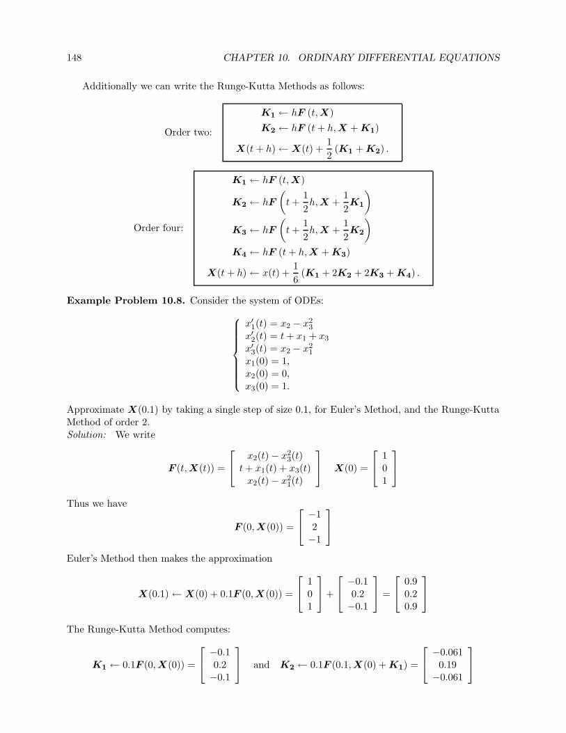
148 CHAPTER 10. ORDINARY DIFFERENTIAL EQUATIONS
Additionally we can write the Runge-Kutta Methods as follows:
Order two:
K1 ← hF (t,X)
K2 ← hF (t+ h,X + K1)
X(t+ h)←X(t) +1
2(K1 + K2) .
Order four:
K1 ← hF (t,X)
K2 ← hF
(
t+1
2h,X +
1
2K1
)
K3 ← hF
(
t+1
2h,X +
1
2K2
)
K4 ← hF (t+ h,X + K3)
X(t+ h)← x(t) +1
6(K1 + 2K2 + 2K3 + K4) .
Example Problem 10.8. Consider the system of ODEs:
x′1(t) = x2 − x23
x′2(t) = t+ x1 + x3
x′3(t) = x2 − x21
x1(0) = 1,x2(0) = 0,x3(0) = 1.
Approximate X(0.1) by taking a single step of size 0.1, for Euler’s Method, and the Runge-KuttaMethod of order 2.Solution: We write
F (t,X(t)) =
x2(t)− x23(t)
t+ x1(t) + x3(t)x2(t)− x2
1(t)
X(0) =
101
Thus we have
F (0,X(0)) =
−12−1
Euler’s Method then makes the approximation
X(0.1)← X(0) + 0.1F (0,X(0)) =
101
+
−0.10.2−0.1
=
0.90.20.9
The Runge-Kutta Method computes:
K1 ← 0.1F (0,X(0)) =
−0.10.2−0.1
and K2 ← 0.1F (0.1,X(0) + K1) =
−0.0610.19−0.061

10.3. SYSTEMS OF ODES 149
Then
X(0.1)←X(0) +1
2(K1 + K2) =
101
+
−0.08050.195−0.0805
=
0.91950.1950.9195
a
10.3.3 It’s Only Systems
The fact we can simply solve systems of ODEs using old methods is good news. It allows us tosolve higher order ODEs. For example, consider the following problem: given f, a, c0, c1, . . . , cn,find x(t) such that
{
x(n)(t) = f(
t, x(t), x′(t), . . . , x(n−1)(t))
,
x(a) = c0, x′(a) = c1, x
′′(a) = c2, . . . , x(n−1)(a) = cn−1.
We can put this in terms of a system by letting
x0 = x, x1 = x′, x2 = x′′, . . . , xn−1 = x(n−1).
Then the ODE plus these n− 1 equations can be written as
x′n−1(t) = f (t, x0(t), x1(t), x2(t), . . . , xn−1(t))x′0(t) = x1(t)x′1(t) = x2(t)...x′n−2(t) = xn−1(t)x0(a) = c0, x1(a) = c1, x2(a) = c2, . . . , xn−1(a) = cn−1.
This is just a system of ODEs that we can solve like any other.
Note that this trick also works on systems of higher order ODEs. That is, we can transformany system of higher order ODEs into a (larger) system of first order ODEs.
Example Problem 10.9. Rewrite the following system as a system of first order ODEs:
x′′(t) = (t/y(t)) + x′(t)− 1y′(t) = 1
(x′(t)+y(t))
x(0) = 1, x′(0) = 0, y(0) = −1
Solution: We let x0 = x, x1 = x′, x2 = y, then we can rewrite as
x′1(t) = (t/x2(t)) + x1(t)− 1x′0(t) = x1(t)x′2(t) = 1
(x1(t)+x2(t))
x0(0) = 1, x1(0) = 0, x2(0) = −1
a

150 CHAPTER 10. ORDINARY DIFFERENTIAL EQUATIONS
10.3.4 It’s Only Autonomous Systems
In fact, we can use a similar trick to get rid of the time-dependence of an ODE. Consider the firstorder system
x′1 = f1 (t, x1, x2, . . . , xn) ,x′2 = f2 (t, x1, x2, . . . , xn) ,x′3 = f3 (t, x1, x2, . . . , xn) ,
...x′n = fn (t, x1, x2, . . . , xn) ,x1(a) = c1, x2(a) = c2, . . . , xn(a) = cn.
We can get rid of the time dependence and thus make the system autonomous by making tanother variable function to be found. We do this by letting x0 = t, then adding the equationsx′0 = 1, and x0(a) = a, to get the system:
x′0 = 1,x′1 = f1 (x0, x1, x2, . . . , xn) ,x′2 = f2 (x0, x1, x2, . . . , xn) ,x′3 = f3 (x0, x1, x2, . . . , xn) ,
...x′n = fn (x0, x1, x2, . . . , xn) ,x0(a) = a, x1(a) = c1, x2(a) = c2, . . . , xn(a) = cn.
An autonomous system can be written in the more elegant form:
{
X′ = F (X)X (a) = C.
Moreover, we can consider the phase curve of an autonomous system.
One can consider X to be the position of a particle which moves through Rn over time. For
an autonomous system of ODEs, the movement of the particle is dependent only on its currentposition and not on time.1 A phase curve is a flow line in the vector field F . You can think ofthe vector field F as being the velocity, at a given point, of a river, the flow of which is timeindependent. Under this analogy, the phase curve is the path of a vessel placed in the river. In ourdeterministic world, phase curves never cross. This is because at the point of crossing, there wouldhave to be two different values of the tangent of the curve, i.e., the vector field would have to havetwo different values at that point.
The following example illustrates the idea of phase curves for autonomous ODE.
Example 10.10. Consider the autonomous system of ODEs, without an initial value:
{
x′1(t) = −2(x2 − 2.4)x′2(t) = 3(x1 − 1.2)
We can rewrite this ODE as
X ′(t) = F (X(t)) .
1Note that if you have converted a system of n equations with a time dependence to an autonomous system, thenthe autonomous system should be considered a particle moving through R
n+1. In this case time becomes one of thedimensions, and thus we speak of position, instead of time.

10.3. SYSTEMS OF ODES 151
This is an autonomous ODE. The associated vector field can be expressed as
F (X) =
[
0 −23 0
]
X +
[
4.8−3.6
]
.
This vector field is plotted in Figure 10.6.
-0.5
0
0.5
1
1.5
2
2.5
3
3.5
4
4.5
-0.5 0 0.5 1 1.5 2 2.5 3 3.5
Figure 10.6: The vector field F (X) is shown in R2. The tips of the vectors are shown as circles.
(Due to budget restrictions, arrowheads were not available for this figure.)
You should verify that this ODE is solved by
X (t) = r
[ √2 cos(
√6t+ t0)√
3 sin(√
6t+ t0)
]
+
[
1.22.4
]
,
for any r ≥ 0, and t0 ∈ (0, 2π] . Given an initial value, the parameters r and t0 are uniquelydetermined. Thus the trajectory of X over time is that of an ellipse in the plane.2 Thus thefamily of such ellipses, taking all r ≥ 0, form the phase curves of this ODE. We would expect the
approximation of an ODE to never cross a phase curve. This is because the phase curve representsthe
Euler’s Method and the second order Runge-Kutta Method were used to approximate the ODEwith initial value
X (0) =
[
1.51.5
]
.
2In the case r = 0, the ellipse is the “trivial” ellipse which consists of a point.

152 CHAPTER 10. ORDINARY DIFFERENTIAL EQUATIONS
-0.5
0
0.5
1
1.5
2
2.5
3
3.5
4
4.5
-0.5 0 0.5 1 1.5 2 2.5 3 3.5
(a) Euler’s Method
-0.5
0
0.5
1
1.5
2
2.5
3
3.5
4
4.5
-0.5 0 0.5 1 1.5 2 2.5 3 3.5
(b) Runge-Kutta Method
Figure 10.7: The simulated phase curves of the system of Example 10.10 are shown for (a) Euler’sMethod and (b) the Runge-Kutta Method of order 2. The Runge-Kutta Method used larger stepsize, but was more accurate. The actual solution to the ODE is an ellipse, thus the “spiralling”observed for Euler’s Method is spurious.

10.3. SYSTEMS OF ODES 153
Euler’s Method was used for step size h = 0.005 for 3000 steps. The Runge-Kutta Method wasemployed with step size h = 0.015 for 3000 steps. The approximations are shown in Figure 10.7.
Given that the actual solution of this initial value problem is an ellipse, we see that Euler’sMethod performed rather poorly, spiralling out from the ellipse. This must be the case for any stepsize, since Euler’s Method steps in the direction tangent to the actual solution; thus every step ofEuler’s Method puts the approximation on an ellipse of larger radius. Smaller stepsize minimizesthis effect, but at greater computational cost.
The Runge-Kutta Method performs much better, and for larger step size. At the given resolu-tion, no spiralling is observable. Thus the Runge-Kutta Method outperforms Euler’s Method, andat lesser computational cost.3
3Because the Runge-Kutta Method of order two requires two evaluations of F , whereas Euler’s Method requiresonly one, per step, it is expected that they would be ‘evenly matched’ when Runge-Kutta Method uses a step sizetwice that of Euler’s Method.

154 CHAPTER 10. ORDINARY DIFFERENTIAL EQUATIONS
Exercises
(10.1) Given the ODE:{
x′(t) = t2 − x2
x(1) = 1
Approximate x(1.1) by using one step of Euler’s Method. Approximate x(1.1) using onestep of the second order Runge-Kutta Method.
(10.2) Given the ODE:
x′1(t) = x1x2 + tx′2(t) = 2x2 − x2
1
x1(1) = 0x2(1) = 3
Approximate X(1.1) by using one step of Euler’s Method. Approximate X(1.1) using onestep of the second order Runge-Kutta Method.
(10.3) Consider the separable ODEx′(t) = x(t)g(t),
for some function g. Use backward’s Euler (or, alternatively, the right endpoint rule forapproximating integrals) to derive the approximation scheme
x(t+ h)← x(t)
1− hg(t+ h).
What could go wrong with using such a scheme?(10.4) Consider the ODE
x′(t) = x(t) + t2.
Using Taylor’s Theorem, derive a higher order approximation scheme to find x(t+ h) basedon x(t), t, and h.
(10.5) Which of the following ODEs can you show are stable? Which are unstable? Which seemambiguous?(a) x′(t) = −x − arctan x (b) x′(t) = 2x + tan x (c) x′(t) = −4x − ex (d) x′(t) = x + x3
(e) x′(t) = t+ cos x(10.6) Rewrite the following higher order ODE as a system of first order ODEs:
x′′(t) = x(t)− sinx′(t),x(0) = 0,x′(0) = π.
(10.7) Rewrite the system of ODEs as a system of first order ODEs
x′′(t) = y(t) + t− x(t),y′(t) = x′(t) + x(t)− 4,x′(0) = 1,x(0) = 2,y(0) = 0.
(10.8) Rewrite the following higher order system of ODEs as a system of first order ODEs:
x′′′(t) = y′′(t)− x′(t),y′′′(t) = x′′(t) + y′(t),x(0) = x′′(0) = y′(0) = −1,x′(0) = y(0) = y′′(0) = 1.

10.3. SYSTEMS OF ODES 155
(10.9) Implement Euler’s Method for approximating the solution to
{
dx(t)dt = f (t, x(t)) ,x(a) = c.
Your m-file should have header line like:function xfin = euler(f,a,c,h,steps)
where xfin should be the approximate solution to the ODE at time a + steps ? h.(a) Run your code with f(t, x) = −x, using a = 0 6= c, and using h ? steps = 1.0. In this
case the actual solution isxfin = ce−1.
This ODE is stable, so your approximation should be good (cf. Example 10.3). Exper-iment with different values of h.
(b) Run your code with f(t, x) = x, using a = 0 6= c, and using h ? steps = 1.0. In thiscase the actual solution is
xfin = ce.
Your actual solution may be a rather poor approximation. Prepare a plot of errorversus h for varying values of h. (cf. Figure 7.1 and Figure 10.2)
(c) Run your code with f(t, x) = 1/ (1− x) , using a = 0, c = 0.1, and using h?steps = 2.0.Plot your approximations for varying values of steps. For example, try steps values of35, 36, and 90, 91. Also try large values of steps, like 100, 500, 1000. Can you guess whatthe actual solution is supposed to look like? Can you explain the poor performance ofEuler’s Method for this ODE?
(10.10) Implement the Runge-Kutta Method of order two for approximating the solution to
{
dx(t)dt = f (t, x(t)) ,x(a) = c.
Your m-file should have header line like:function xfin = rkm(f,a,c,h,steps)
where xfin should be the approximate solution to the ODE at time a + steps ? h.Test your code with the ODEs from the previous problem. Does the Runge-Kutta Methodperform any better than Euler’s Method for the last ODE?

156 CHAPTER 10. ORDINARY DIFFERENTIAL EQUATIONS
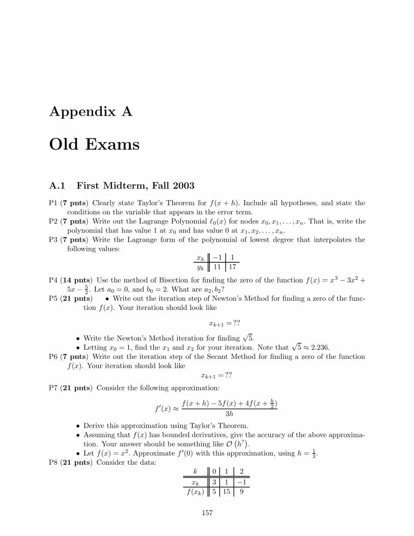
Appendix A
Old Exams
A.1 First Midterm, Fall 2003
P1 (7 pnts) Clearly state Taylor’s Theorem for f(x + h). Include all hypotheses, and state theconditions on the variable that appears in the error term.
P2 (7 pnts) Write out the Lagrange Polynomial `0(x) for nodes x0, x1, . . . , xn. That is, write thepolynomial that has value 1 at x0 and has value 0 at x1, x2, . . . , xn.
P3 (7 pnts) Write the Lagrange form of the polynomial of lowest degree that interpolates thefollowing values:
xk −1 1
yk 11 17
P4 (14 pnts) Use the method of Bisection for finding the zero of the function f(x) = x3 − 3x2 +5x− 5
2 . Let a0 = 0, and b0 = 2. What are a2, b2?P5 (21 pnts) • Write out the iteration step of Newton’s Method for finding a zero of the func-
tion f(x). Your iteration should look like
xk+1 =??
• Write the Newton’s Method iteration for finding√
5.• Letting x0 = 1, find the x1 and x2 for your iteration. Note that
√5 ≈ 2.236.
P6 (7 pnts) Write out the iteration step of the Secant Method for finding a zero of the functionf(x). Your iteration should look like
xk+1 =??
P7 (21 pnts) Consider the following approximation:
f ′(x) ≈ f(x+ h)− 5f(x) + 4f(x+ h2 )
3h
• Derive this approximation using Taylor’s Theorem.• Assuming that f(x) has bounded derivatives, give the accuracy of the above approxima-
tion. Your answer should be something like O(
h?)
.• Let f(x) = x2. Approximate f ′(0) with this approximation, using h = 1
3 .P8 (21 pnts) Consider the data:
k 0 1 2
xk 3 1 −1
f(xk) 5 15 9
157

158 APPENDIX A. OLD EXAMS
• Construct the divided differences table for the data.• Construct the Newton form of the polynomial p(x) of lowest degree that interpolatesf(x) at these nodes.
• Suppose that these data were generated by the function f(x) = x3 − 5x2 + 2x + 17.Find a numerical upper bound on the error |p(x)− f(x)| over the interval [−1, 3]. Youranswer should be a number.
A.2 Second Midterm, Fall 2003
P1 (6 pnts) Write the Trapezoid rule approximation for∫ ba f(x) dx, using the nodes {xi}ni=0.
P2 (6 pnts) Suppose Gaussian Elimination with scaled partial pivoting is applied to the matrix
A =
0.0001 −0.1 −0.01 0.00143 91 −43 1−12 26 −1 0−7 1
2 −10 π
.
Which row contains the first pivot? You must show your work.P3 (14 pnts) Let φ(n) be some quadrature rule that divides an interval into 2n equal subintervals.
Suppose∫ b
af(x) dx = φ(n) + a5h
5n + a10h
10n + a15h
15n + . . . ,
where hn = b−a2n . Using evaluations of φ(·), devise a “Romberg-style” quadrature rule that is
a O(
h10n
)
approximation to the integral.P4 (14 pnts) Compute the LU factorization of the matrix
A =
1 0 −10 2 02 2 −1
using naıve Gaussian Elimination. Show all your work. Your final answer should be twomatrices, L and U. Verify your answer, i.e., verify that A = LU.
P5 (14 pnts) Run one iteration of either Jacobi or Gauss Seidel on the system:
1 3 4−2 2 1−1 3 −2
x =
−3−3
1
Start with x(0) = [1 1 1]> . Clearly indicate your answer x(1). Show your work. You mustindicate which of the two methods you are using.
P6 (21 pnts) Derive the two-node Chebyshev Quadrature rule:
∫ 1
−1f(x) dx ≈ c [f(x0) + f(x1)] .
Make this rule exact for all polynomials of degree ≤ 2.P7 (28 pnts) Consider the quadrature rule:
∫ 1
0f(x) dx ≈ z0f(0) + z1f(1) + z2f
′(0) + z3f′(1).

A.3. FINAL EXAM, FALL 2003 159
• Write four linear equations involving zi to make this rule exact for polynomials of thehighest possible degree.
• Solve your system for z using naıve Gaussian Elimination.
A.3 Final Exam, Fall 2003
P1 (4 pnts) Clearly state Taylor’s Theorem for f(x + h). Include all hypotheses, and state theconditions on the variable that appears in the error term.
P2 (4 pnts) State the conditions that characterize S(x) as a natural cubic spline on the interval[a, b]. Let the knots be a = t0 < t1 < t2 < . . . < tn = b.
P3 (4 pnts) Let x0 = 3, x1 = −5, x2 = 0. Write out the Lagrange Polynomial `0(x) for thesenodes; that is, write the polynomial that has value 1 at x0 and has value 0 at x1, x2.
P4 (4 pnts) Consider the ODE:{
x′(t) = f(t, x(t))x(a) = c
Write out the Euler Method to step from x(t) to x(t+ h).P5 (7 pnts) Compute the LU factorization of the matrix
A =
−1 1 01 1 −1−2 0 2
using naıve Gaussian Elimination. Show all your work. Your final answer should be twomatrices, L and U. Verify your answer, i.e., verify that A = LU.
P6 (9 pnts) Let α be given. Determine a quadrature rule of the form∫ α
−αf(x) dx ≈ Af(0) +Bf ′′(−α) + Cf ′′(α)
that is exact for polynomials of highest possible degree. What is the highest degree polynomialfor which this rule is exact?
P7 (9 pnts) Suppose that φ(n) is some computational function that approximates a desired quan-tity, L. Furthermore suppose that
φ(n) = L+ a1n− 1
2 + a2n− 2
2 + a3n− 3
2 + . . .
Combine two evaluations of φ(·) in the manner of Richardson to get a O(
n−1)
approximationto L.
P8 (9 pnts) Find the least-squares best approximate of the form y = ln (cx) to the data
x0 x1 . . . xn
y0 y1 . . . yn
Caution: this should not be done with basis vectors.P9 (9 pnts) Let
F = {f(x) = c0x+ c1 log x+ c2 cos x | c0, c1, c2 ∈ R } .Set up (but do not attempt to solve) the normal equations to find the least-squares best f ∈ Fto approximate the data:
x0 x1 . . . xn
y0 y1 . . . yn

160 APPENDIX A. OLD EXAMS
The normal equations should involve the vector c = [c0 c1 c2]>, which uniquely determines a
function in F .P10 (9 pnts) Consider the following approximation:
f ′′(x) ≈ 3f(x− h)− 4f(x) + f(x+ 3h)
6h2
• Derive this approximation using Taylor’s Theorem.• Assuming that f(x) has bounded derivatives, give the accuracy of the above approxima-
tion. Your answer should be something like O(
h?)
.P11 (11 pnts) Consider the ODE:
{
x′(t) = x(t)g(t)x(0) = 1
• Use the Fundamental Theorem of Calculus to write a step update of the form:
x(t+ h) = x(t) +
∫ t+h
t??
• Approximate the integral using the Trapezoid Rule to get an explicit step update of theform
x(t+ h)← Q(t, x(t), h)
• Suppose that g(t) ≥ m > 0 for all t. Do you see any problem with this stepping methodif h > 2/m?Hint: the actual solution to the ODE is
x(t) = eR
t
0g(r) dr.
P12 (9 pnts) Consider the ODE:
{
x′(t) = ex(t) + sin (x(t))x(0) = 0
Write out the Taylor’s series method of order three to approximate x(t+ h) given x(t). It ispermissible to write the update as a small program like:
x′(t) ← Q0(x(t))
x′′(t) ← Q1(x(t), x′(t))
...
x(t+ h) ← R(x(t), x′(t), x′′(t), . . .)
rather than write the update as a monstrous equation of the form
x(t+ h)←M(x(t)).
P13 (15 pnts) Consider the data:k 0 1 2
xk −0.5 0 0.5
f(xk) 5 15 9
• Construct the divided differences table for the data.
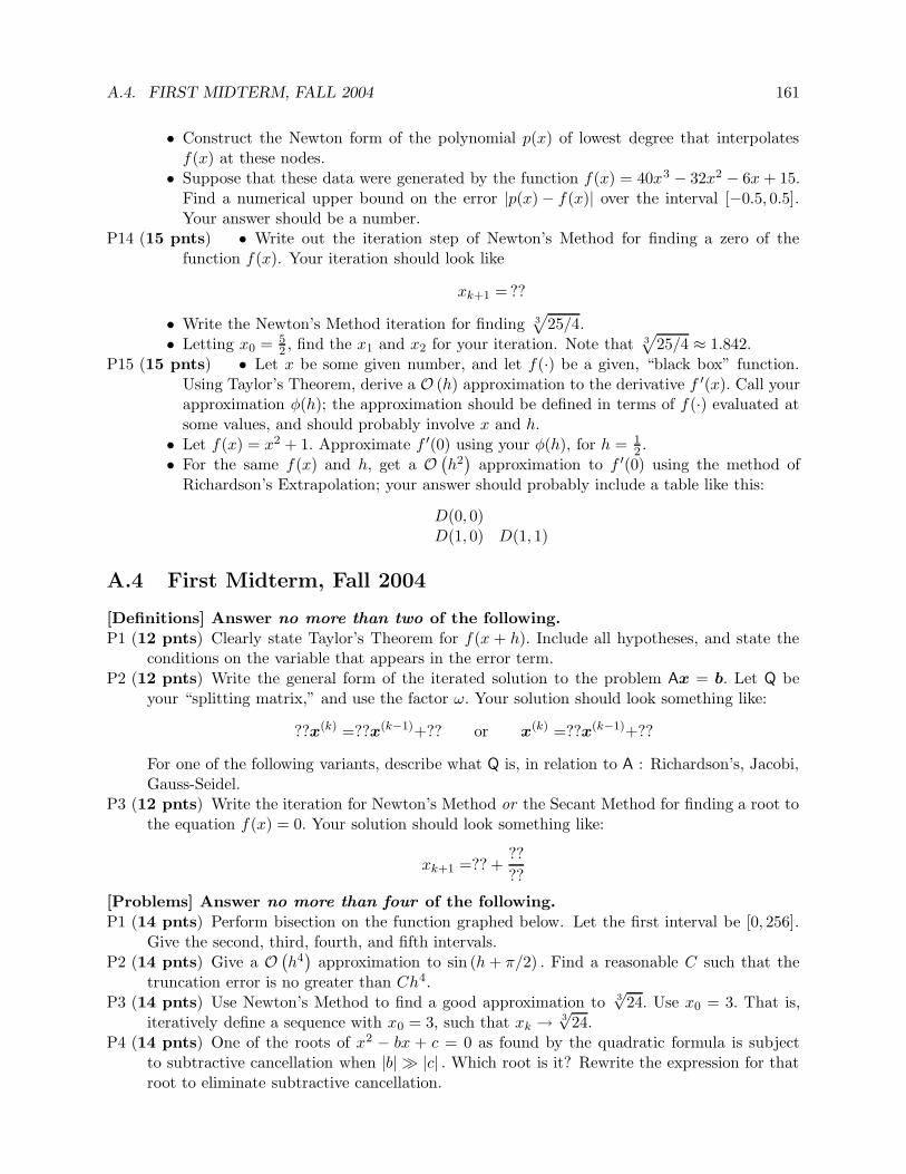
A.4. FIRST MIDTERM, FALL 2004 161
• Construct the Newton form of the polynomial p(x) of lowest degree that interpolatesf(x) at these nodes.
• Suppose that these data were generated by the function f(x) = 40x3 − 32x2 − 6x+ 15.Find a numerical upper bound on the error |p(x)− f(x)| over the interval [−0.5, 0.5].Your answer should be a number.
P14 (15 pnts) • Write out the iteration step of Newton’s Method for finding a zero of thefunction f(x). Your iteration should look like
xk+1 =??
• Write the Newton’s Method iteration for finding 3√
25/4.• Letting x0 = 5
2 , find the x1 and x2 for your iteration. Note that 3√
25/4 ≈ 1.842.P15 (15 pnts) • Let x be some given number, and let f(·) be a given, “black box” function.
Using Taylor’s Theorem, derive a O (h) approximation to the derivative f ′(x). Call yourapproximation φ(h); the approximation should be defined in terms of f(·) evaluated atsome values, and should probably involve x and h.
• Let f(x) = x2 + 1. Approximate f ′(0) using your φ(h), for h = 12 .
• For the same f(x) and h, get a O(
h2)
approximation to f ′(0) using the method ofRichardson’s Extrapolation; your answer should probably include a table like this:
D(0, 0)D(1, 0) D(1, 1)
A.4 First Midterm, Fall 2004
[Definitions] Answer no more than two of the following.P1 (12 pnts) Clearly state Taylor’s Theorem for f(x + h). Include all hypotheses, and state the
conditions on the variable that appears in the error term.P2 (12 pnts) Write the general form of the iterated solution to the problem Ax = b. Let Q be
your “splitting matrix,” and use the factor ω. Your solution should look something like:
??x(k) =??x(k−1)+?? or x(k) =??x(k−1)+??
For one of the following variants, describe what Q is, in relation to A : Richardson’s, Jacobi,Gauss-Seidel.
P3 (12 pnts) Write the iteration for Newton’s Method or the Secant Method for finding a root tothe equation f(x) = 0. Your solution should look something like:
xk+1 =?? +??
??
[Problems] Answer no more than four of the following.P1 (14 pnts) Perform bisection on the function graphed below. Let the first interval be [0, 256].
Give the second, third, fourth, and fifth intervals.P2 (14 pnts) Give a O
(
h4)
approximation to sin (h+ π/2) . Find a reasonable C such that thetruncation error is no greater than Ch4.
P3 (14 pnts) Use Newton’s Method to find a good approximation to 3√
24. Use x0 = 3. That is,iteratively define a sequence with x0 = 3, such that xk → 3
√24.
P4 (14 pnts) One of the roots of x2 − bx + c = 0 as found by the quadratic formula is subjectto subtractive cancellation when |b| � |c| . Which root is it? Rewrite the expression for thatroot to eliminate subtractive cancellation.

162 APPENDIX A. OLD EXAMS
0 32 64 96 128 160 192 224 256
-64
-32
0
32
64
P5 (14 pnts) Find the LU decomposition of the following matrix by Gaussian Elimination withnaıve pivoting.
3 2 4−6 1 −612 −12 10
P6 (14 pnts) Consider the linear equation:
6 1 12 4 01 2 6
x =
5−6
3
Letting x(0) = [1 1 1]>, find x(1) using either the Gauss-Seidel or Jacobi iterative schemes.Use weighting ω = 1. You must indicate which scheme you are using. Show all your work.
[Questions] Answer only one of the following.
P1 (20 pnts) Suppose that the eigenvalues of A are in [α, β] with 0 < α < β. Find the ω thatminimizes
∥
∥I− ωA2∥
∥
2. What is the minimal value of
∥
∥I− ωA2∥
∥
2for this optimal ω? For full
credit you need to make some argument why this ω minimizes this norm.P2 (20 pnts) Let f(x) = 0 have a unique root r. Recall that the form of the error for Newton’s
Method is
ek+1 =−f ′′(ξk)2f ′(xk)
e2k,
where ek = r − xk. Suppose that f(x) has the properties that f ′(x) ≥ m > 0 for all x, and|f ′′(x)| ≤M for all x. Find δ > 0 such that |ek| < δ insures that xn → r. Justify your answer.
P3 (20 pnts) Suppose that f(r) = 0 = f ′(r) 6= f ′′(r), and f ′′(x) is continuous. Letting ek = xk−r,show that for Newton’s Method,
ek+1 ≈1
2ek,
when |ek| is sufficiently small. (Hint: Use Taylor’s Theorem twice.) Is this faster or slowerconvergence than for Newton’s Method with a simple root?
A.5 Second Midterm, Fall 2004
[Definitions] Answer no more than two of the following three.
P1 (10 pnts) For a set of distinct nodes x0, x1, . . . , x13, what is the Lagrange Polynomial `5(x)?You may write your answer as a product. What degree is this polynomial?
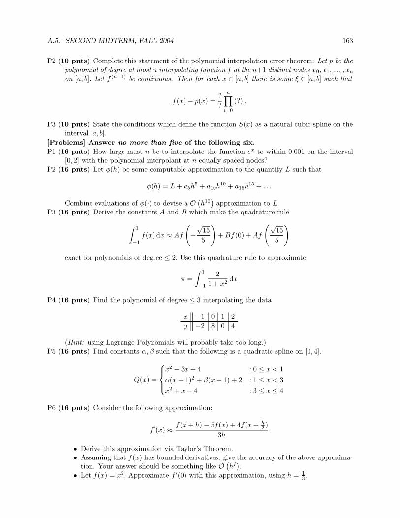
A.5. SECOND MIDTERM, FALL 2004 163
P2 (10 pnts) Complete this statement of the polynomial interpolation error theorem: Let p be the
polynomial of degree at most n interpolating function f at the n+1 distinct nodes x0, x1, . . . , xn
on [a, b]. Let f (n+1) be continuous. Then for each x ∈ [a, b] there is some ξ ∈ [a, b] such that
f(x)− p(x) =?
?
n∏
i=0
(?) .
P3 (10 pnts) State the conditions which define the function S(x) as a natural cubic spline on theinterval [a, b].
[Problems] Answer no more than five of the following six.
P1 (16 pnts) How large must n be to interpolate the function ex to within 0.001 on the interval[0, 2] with the polynomial interpolant at n equally spaced nodes?
P2 (16 pnts) Let φ(h) be some computable approximation to the quantity L such that
φ(h) = L+ a5h5 + a10h
10 + a15h15 + . . .
Combine evaluations of φ(·) to devise a O(
h10)
approximation to L.P3 (16 pnts) Derive the constants A and B which make the quadrature rule
∫ 1
−1f(x) dx ≈ Af
(
−√
15
5
)
+Bf(0) +Af
(√15
5
)
exact for polynomials of degree ≤ 2. Use this quadrature rule to approximate
π =
∫ 1
−1
2
1 + x2dx
P4 (16 pnts) Find the polynomial of degree ≤ 3 interpolating the data
x −1 0 1 2
y −2 8 0 4
(Hint: using Lagrange Polynomials will probably take too long.)P5 (16 pnts) Find constants α, β such that the following is a quadratic spline on [0, 4].
Q(x) =
x2 − 3x+ 4 : 0 ≤ x < 1
α(x− 1)2 + β(x− 1) + 2 : 1 ≤ x < 3
x2 + x− 4 : 3 ≤ x ≤ 4
P6 (16 pnts) Consider the following approximation:
f ′(x) ≈ f(x+ h)− 5f(x) + 4f(x+ h2 )
3h
• Derive this approximation via Taylor’s Theorem.• Assuming that f(x) has bounded derivatives, give the accuracy of the above approxima-
tion. Your answer should be something like O(
h?)
.• Let f(x) = x2. Approximate f ′(0) with this approximation, using h = 1
3 .

164 APPENDIX A. OLD EXAMS
A.6 Final Exam, Fall 2004
[Definitions] Answer all of the following.P1 (10 pnts) Clearly state Taylor’s Theorem for f(x + h). Include all hypotheses, and state the
conditions on the variable that appears in the error term.P2 (10 pnts) Write the iteration for Newton’s Method or the Secant Method for finding a root to
the equation f(x) = 0. Your solution should look something like:
xk+1 =?? +??
??
P3 (10 pnts) Write the general form of the iterated solution to the problem Ax = b. Let Q beyour “splitting matrix,” and use the factor ω. Your solution should look something like:
??x(k) =??x(k−1)+?? or x(k) =??x(k−1)+??
For one of the following variants, describe what Q is, in relation to A : Richardson’s, Jacobi,Gauss-Seidel.
P4 (10 pnts) Define what it means for the function f(x) ∈ F to be the least squares best approx-imant to the data
x0 x1 . . . xn
y0 y1 . . . yn
[Problems] Answer all of the following.P1 (10 pnts) Rewrite this system of higher order ODEs as a system of first order ODEs:
x′′(t) = x′(t) [x(t) + ty(t)]
y′′(t) = y′(t) [y(t)− tx(t)]x′(0) = 1
x(0) = 4
y′(0) = −3
y(0) = −2
P2 (10 pnts) Consider the ODE:{
x′(t) = t (x+ 1)2
x(2) = 1/2
Use Euler’s Method to find an approximate value of x(2.1) using a single step.P3 (10 pnts) Let φ(h) be some computable approximation to the quantity L such that
φ(h) = L+ a4h4 + a8h
8 + a12h12 + . . .
Combine evaluations of φ(·) to devise a O(
h8)
approximation to L.P4 (15 pnts) Consider the approximation
f ′(x) ≈ 9f(x+ h)− 8f(x)− f(x− 3h)
12h
(a) Derive this approximation using Taylor’s Theorem.(b) Assuming that f(x) has bounded derivatives, give the accuracy of the above approxima-
tion. Your answer should be something like O(
h?)
.

A.6. FINAL EXAM, FALL 2004 165
P5 (15 pnts) Find constants, α, β, γ such that the following is a natural cubic spline on [1, 3].
Q(x) =
{
α (x− 1)3 + β (x− 1)2 + 12 (x− 1) + 1 : 1 ≤ x < 2
γx3 + 18x2 − 30x+ 19 : 2 ≤ x < 3
P6 (15 pnts) Devise a subroutine that, given an input number z, calculates an approximate to 3√z
via Newton’s Method. Write your subroutine in pseudo code, Matlab, or C/C++. Includereasonable termination conditions so your subroutine will terminate if it finds a good approx-imate solution. Your subroutine should use only the basic arithmetic operations of addition,subtraction, multiplication, division; in particular your subroutine should not have access toa cubed root or logarithm operator.
P7 (15 pnts) Consider the ODE:{
x′(t) = cos (x(t)) + sin (x(t))
x(0) = 1
Use Taylor’s theorem to devise a O(
h3)
approximant to x(t+ h) which is a function of x, t,and h only. You may write your answer as a program:
x′(t)← Q0(x(t))
x′′(t)← Q1(x(t), x′(t))
...
x← R(x(t), x′(t), x′′(t), . . .)
such that x(t+ h) = x+O(
h3)
.[Questions] Answer all of the following.P1 (20 pnts) Consider the “quadrature” rule:
∫ 1
0f(x) dx ≈ A0f(0) +A1f(1) +A2f
′(1) +A3f′′(1)
(a) Write four linear equations involving Ai to make this rule exact for polynomials of thehighest possible degree.
(b) Find the constants Ai using Gaussian Elimination with naıve pivoting.P2 (20 pnts) Consider the data:
k 0 1 2
xk 0 0.25 0.5
f(xk) 1.5 1 0.5
(a) Construct the divided differences table for the data.(b) Construct the Newton form of the polynomial p(x) of lowest degree that interpolates
f(x) at these nodes.(c) What degree is your polynomial? Is this strange?(d) Suppose that these data were generated by the function
f(x) = 1 +cos 2πx
2.
Find an upper bound on the error |p(x)− f(x)| over the interval [0, 0.5]. Your answershould be a number.

166 APPENDIX A. OLD EXAMS
P3 (20 pnts) LetF =
{
f(x) = c0√x+ c1`(x) + c2e
x | c0, c1, c2 ∈ R}
,
where `(x) is some black box function. We are concerned with finding the least-squares bestf ∈ F to approximate the data
x0 x1 . . . xn
y0 y1 . . . yn
(a) Set up (but do not attempt to solve) the normal equations to find the the vector c =[c0 c1 c2]
>, which determines the least squares approximant in F .(b) Now suppose that the function `(x) happens to be the Lagrange Polynomial associated
with x7, among the values x0, x1, . . . , xn. That is, `(xj) = δj7. Prove that f(x7) = y7,where f is the least squares best approximant to the data.
P4 (10 pnts) State some substantive question which you thought might appear on this exam, butdid not. Answer this question (correctly).
Appendix B
GNU Free Documentation License
Version 1.2, November 2002Copyright c©2000,2001,2002 Free Software Foundation, Inc.
59 Temple Place, Suite 330, Boston, MA 02111-1307 USA
Everyone is permitted to copy and distribute verbatim copies of this license document, but changing it is not allowed.
Preamble
The purpose of this License is to make a manual, textbook, or other functional and useful document ”free” in the sense offreedom: to assure everyone the effective freedom to copy and redistribute it, with or without modifying it, either commerciallyor noncommercially. Secondarily, this License preserves for the author and publisher a way to get credit for their work, whilenot being considered responsible for modifications made by others.
This License is a kind of ”copyleft”, which means that derivative works of the document must themselves be free in thesame sense. It complements the GNU General Public License, which is a copyleft license designed for free software.
We have designed this License in order to use it for manuals for free software, because free software needs free documentation:a free program should come with manuals providing the same freedoms that the software does. But this License is not limitedto software manuals; it can be used for any textual work, regardless of subject matter or whether it is published as a printedbook. We recommend this License principally for works whose purpose is instruction or reference.
1. APPLICABILITY AND DEFINITIONS
This License applies to any manual or other work, in any medium, that contains a notice placed by the copyright holdersaying it can be distributed under the terms of this License. Such a notice grants a world-wide, royalty-free license, unlimitedin duration, to use that work under the conditions stated herein. The ”Document”, below, refers to any such manual or work.Any member of the public is a licensee, and is addressed as ”you”. You accept the license if you copy, modify or distribute thework in a way requiring permission under copyright law.
A ”Modified Version” of the Document means any work containing the Document or a portion of it, either copiedverbatim, or with modifications and/or translated into another language.
A ”Secondary Section” is a named appendix or a front-matter section of the Document that deals exclusively with therelationship of the publishers or authors of the Document to the Document’s overall subject (or to related matters) and containsnothing that could fall directly within that overall subject. (Thus, if the Document is in part a textbook of mathematics, aSecondary Section may not explain any mathematics.) The relationship could be a matter of historical connection with thesubject or with related matters, or of legal, commercial, philosophical, ethical or political position regarding them.
The ”Invariant Sections” are certain Secondary Sections whose titles are designated, as being those of Invariant Sections,in the notice that says that the Document is released under this License. If a section does not fit the above definition of Secondarythen it is not allowed to be designated as Invariant. The Document may contain zero Invariant Sections. If the Document doesnot identify any Invariant Sections then there are none.
The ”Cover Texts” are certain short passages of text that are listed, as Front-Cover Texts or Back-Cover Texts, inthe notice that says that the Document is released under this License. A Front-Cover Text may be at most 5 words, and aBack-Cover Text may be at most 25 words.
A ”Transparent” copy of the Document means a machine-readable copy, represented in a format whose specification isavailable to the general public, that is suitable for revising the document straightforwardly with generic text editors or (forimages composed of pixels) generic paint programs or (for drawings) some widely available drawing editor, and that is suitablefor input to text formatters or for automatic translation to a variety of formats suitable for input to text formatters. A copymade in an otherwise Transparent file format whose markup, or absence of markup, has been arranged to thwart or discouragesubsequent modification by readers is not Transparent. An image format is not Transparent if used for any substantial amountof text. A copy that is not ”Transparent” is called ”Opaque”.
167
168 APPENDIX B. GNU FREE DOCUMENTATION LICENSE
Examples of suitable formats for Transparent copies include plain ASCII without markup, Texinfo input format, LaTeXinput format, SGML or XML using a publicly available DTD, and standard-conforming simple HTML, PostScript or PDFdesigned for human modification. Examples of transparent image formats include PNG, XCF and JPG. Opaque formatsinclude proprietary formats that can be read and edited only by proprietary word processors, SGML or XML for which theDTD and/or processing tools are not generally available, and the machine-generated HTML, PostScript or PDF produced bysome word processors for output purposes only.
The ”Title Page” means, for a printed book, the title page itself, plus such following pages as are needed to hold, legibly,the material this License requires to appear in the title page. For works in formats which do not have any title page as such,”Title Page” means the text near the most prominent appearance of the work’s title, preceding the beginning of the body ofthe text.
A section ”Entitled XYZ” means a named subunit of the Document whose title either is precisely XYZ or contains XYZin parentheses following text that translates XYZ in another language. (Here XYZ stands for a specific section name mentionedbelow, such as ”Acknowledgements”, ”Dedications”, ”Endorsements”, or ”History”.) To ”Preserve the Title” ofsuch a section when you modify the Document means that it remains a section ”Entitled XYZ” according to this definition.
The Document may include Warranty Disclaimers next to the notice which states that this License applies to the Document.These Warranty Disclaimers are considered to be included by reference in this License, but only as regards disclaiming warranties:any other implication that these Warranty Disclaimers may have is void and has no effect on the meaning of this License.
2. VERBATIM COPYING
You may copy and distribute the Document in any medium, either commercially or noncommercially, provided that thisLicense, the copyright notices, and the license notice saying this License applies to the Document are reproduced in all copies,and that you add no other conditions whatsoever to those of this License. You may not use technical measures to obstruct orcontrol the reading or further copying of the copies you make or distribute. However, you may accept compensation in exchangefor copies. If you distribute a large enough number of copies you must also follow the conditions in section 3.
You may also lend copies, under the same conditions stated above, and you may publicly display copies.
3. COPYING IN QUANTITY
If you publish printed copies (or copies in media that commonly have printed covers) of the Document, numbering morethan 100, and the Document’s license notice requires Cover Texts, you must enclose the copies in covers that carry, clearly andlegibly, all these Cover Texts: Front-Cover Texts on the front cover, and Back-Cover Texts on the back cover. Both covers mustalso clearly and legibly identify you as the publisher of these copies. The front cover must present the full title with all words ofthe title equally prominent and visible. You may add other material on the covers in addition. Copying with changes limited tothe covers, as long as they preserve the title of the Document and satisfy these conditions, can be treated as verbatim copyingin other respects.
If the required texts for either cover are too voluminous to fit legibly, you should put the first ones listed (as many as fitreasonably) on the actual cover, and continue the rest onto adjacent pages.
If you publish or distribute Opaque copies of the Document numbering more than 100, you must either include a machine-readable Transparent copy along with each Opaque copy, or state in or with each Opaque copy a computer-network location fromwhich the general network-using public has access to download using public-standard network protocols a complete Transparentcopy of the Document, free of added material. If you use the latter option, you must take reasonably prudent steps, when youbegin distribution of Opaque copies in quantity, to ensure that this Transparent copy will remain thus accessible at the statedlocation until at least one year after the last time you distribute an Opaque copy (directly or through your agents or retailers)of that edition to the public.
It is requested, but not required, that you contact the authors of the Document well before redistributing any large numberof copies, to give them a chance to provide you with an updated version of the Document.
4. MODIFICATIONS
You may copy and distribute a Modified Version of the Document under the conditions of sections 2 and 3 above, providedthat you release the Modified Version under precisely this License, with the Modified Version filling the role of the Document,thus licensing distribution and modification of the Modified Version to whoever possesses a copy of it. In addition, you mustdo these things in the Modified Version:
A. Use in the Title Page (and on the covers, if any) a title distinct from that of the Document, and from those of previousversions (which should, if there were any, be listed in the History section of the Document). You may use the same titleas a previous version if the original publisher of that version gives permission.
B. List on the Title Page, as authors, one or more persons or entities responsible for authorship of the modifications in theModified Version, together with at least five of the principal authors of the Document (all of its principal authors, if ithas fewer than five), unless they release you from this requirement.
C. State on the Title page the name of the publisher of the Modified Version, as the publisher.
D. Preserve all the copyright notices of the Document.
E. Add an appropriate copyright notice for your modifications adjacent to the other copyright notices.

169
F. Include, immediately after the copyright notices, a license notice giving the public permission to use the Modified Versionunder the terms of this License, in the form shown in the Addendum below.
G. Preserve in that license notice the full lists of Invariant Sections and required Cover Texts given in the Document’slicense notice.
H. Include an unaltered copy of this License.
I. Preserve the section Entitled ”History”, Preserve its Title, and add to it an item stating at least the title, year, newauthors, and publisher of the Modified Version as given on the Title Page. If there is no section Entitled ”History” inthe Document, create one stating the title, year, authors, and publisher of the Document as given on its Title Page,then add an item describing the Modified Version as stated in the previous sentence.
J. Preserve the network location, if any, given in the Document for public access to a Transparent copy of the Document,and likewise the network locations given in the Document for previous versions it was based on. These may be placedin the ”History” section. You may omit a network location for a work that was published at least four years before theDocument itself, or if the original publisher of the version it refers to gives permission.
K. For any section Entitled ”Acknowledgements” or ”Dedications”, Preserve the Title of the section, and preserve in thesection all the substance and tone of each of the contributor acknowledgements and/or dedications given therein.
L. Preserve all the Invariant Sections of the Document, unaltered in their text and in their titles. Section numbers or theequivalent are not considered part of the section titles.
M. Delete any section Entitled ”Endorsements”. Such a section may not be included in the Modified Version.
N. Do not retitle any existing section to be Entitled ”Endorsements” or to conflict in title with any Invariant Section.
O. Preserve any Warranty Disclaimers.
If the Modified Version includes new front-matter sections or appendices that qualify as Secondary Sections and containno material copied from the Document, you may at your option designate some or all of these sections as invariant. To do this,add their titles to the list of Invariant Sections in the Modified Version’s license notice. These titles must be distinct from anyother section titles.
You may add a section Entitled ”Endorsements”, provided it contains nothing but endorsements of your Modified Version byvarious parties–for example, statements of peer review or that the text has been approved by an organization as the authoritativedefinition of a standard.
You may add a passage of up to five words as a Front-Cover Text, and a passage of up to 25 words as a Back-Cover Text,to the end of the list of Cover Texts in the Modified Version. Only one passage of Front-Cover Text and one of Back-CoverText may be added by (or through arrangements made by) any one entity. If the Document already includes a cover text forthe same cover, previously added by you or by arrangement made by the same entity you are acting on behalf of, you may notadd another; but you may replace the old one, on explicit permission from the previous publisher that added the old one.
The author(s) and publisher(s) of the Document do not by this License give permission to use their names for publicityfor or to assert or imply endorsement of any Modified Version.
5. COMBINING DOCUMENTS
You may combine the Document with other documents released under this License, under the terms defined in section 4above for modified versions, provided that you include in the combination all of the Invariant Sections of all of the originaldocuments, unmodified, and list them all as Invariant Sections of your combined work in its license notice, and that you preserveall their Warranty Disclaimers.
The combined work need only contain one copy of this License, and multiple identical Invariant Sections may be replacedwith a single copy. If there are multiple Invariant Sections with the same name but different contents, make the title of eachsuch section unique by adding at the end of it, in parentheses, the name of the original author or publisher of that section ifknown, or else a unique number. Make the same adjustment to the section titles in the list of Invariant Sections in the licensenotice of the combined work.
In the combination, you must combine any sections Entitled ”History” in the various original documents, forming one sectionEntitled ”History”; likewise combine any sections Entitled ”Acknowledgements”, and any sections Entitled ”Dedications”. Youmust delete all sections Entitled ”Endorsements”.
6. COLLECTIONS OF DOCUMENTS
You may make a collection consisting of the Document and other documents released under this License, and replace theindividual copies of this License in the various documents with a single copy that is included in the collection, provided thatyou follow the rules of this License for verbatim copying of each of the documents in all other respects.
You may extract a single document from such a collection, and distribute it individually under this License, provided youinsert a copy of this License into the extracted document, and follow this License in all other respects regarding verbatimcopying of that document.
7. AGGREGATION WITH INDEPENDENT WORKS
170 APPENDIX B. GNU FREE DOCUMENTATION LICENSE
A compilation of the Document or its derivatives with other separate and independent documents or works, in or on avolume of a storage or distribution medium, is called an ”aggregate” if the copyright resulting from the compilation is not usedto limit the legal rights of the compilation’s users beyond what the individual works permit. When the Document is includedin an aggregate, this License does not apply to the other works in the aggregate which are not themselves derivative works ofthe Document.
If the Cover Text requirement of section 3 is applicable to these copies of the Document, then if the Document is less thanone half of the entire aggregate, the Document’s Cover Texts may be placed on covers that bracket the Document within theaggregate, or the electronic equivalent of covers if the Document is in electronic form. Otherwise they must appear on printedcovers that bracket the whole aggregate.
8. TRANSLATION
Translation is considered a kind of modification, so you may distribute translations of the Document under the terms ofsection 4. Replacing Invariant Sections with translations requires special permission from their copyright holders, but you mayinclude translations of some or all Invariant Sections in addition to the original versions of these Invariant Sections. You mayinclude a translation of this License, and all the license notices in the Document, and any Warranty Disclaimers, provided thatyou also include the original English version of this License and the original versions of those notices and disclaimers. In caseof a disagreement between the translation and the original version of this License or a notice or disclaimer, the original versionwill prevail.
If a section in the Document is Entitled ”Acknowledgements”, ”Dedications”, or ”History”, the requirement (section 4) toPreserve its Title (section 1) will typically require changing the actual title.
9. TERMINATION
You may not copy, modify, sublicense, or distribute the Document except as expressly provided for under this License.Any other attempt to copy, modify, sublicense or distribute the Document is void, and will automatically terminate your rightsunder this License. However, parties who have received copies, or rights, from you under this License will not have their licensesterminated so long as such parties remain in full compliance.
10. FUTURE REVISIONS OF THIS LICENSE
The Free Software Foundation may publish new, revised versions of the GNU Free Documentation License from time totime. Such new versions will be similar in spirit to the present version, but may differ in detail to address new problems orconcerns. See http://www.gnu.org/copyleft/.
Each version of the License is given a distinguishing version number. If the Document specifies that a particular numberedversion of this License ”or any later version” applies to it, you have the option of following the terms and conditions either ofthat specified version or of any later version that has been published (not as a draft) by the Free Software Foundation. If theDocument does not specify a version number of this License, you may choose any version ever published (not as a draft) by theFree Software Foundation.
ADDENDUM: How to use this License for your documents
To use this License in a document you have written, include a copy of the License in the document and put the followingcopyright and license notices just after the title page:
Copyright c©YEAR YOUR NAME. Permission is granted to copy, distribute and/or modify this documentunder the terms of the GNU Free Documentation License, Version 1.2 or any later version published by the FreeSoftware Foundation; with no Invariant Sections, no Front-Cover Texts, and no Back-Cover Texts. A copy ofthe license is included in the section entitled ”GNU Free Documentation License”.
If you have Invariant Sections, Front-Cover Texts and Back-Cover Texts, replace the ”with...Texts.” line with this:
with the Invariant Sections being LIST THEIR TITLES, with the Front-Cover Texts being LIST, and with theBack-Cover Texts being LIST.
If you have Invariant Sections without Cover Texts, or some other combination of the three, merge those two alternativesto suit the situation.
If your document contains nontrivial examples of program code, we recommend releasing these examples in parallel underyour choice of free software license, such as the GNU General Public License, to permit their use in free software.

Bibliography
[1] Guillaume Bal. Lecture notes, course on numerical analysis, 2002. URLhttp://www.columbia.edu/~gb2030/COURSES/E6302/NumAnal.ps.
[2] Samuel Daniel Conte and Carl de Boor. Elementary Numerical Analysis; An Algorithmic Ap-
proach. McGraw-Hill, New York, third edition, 1980. ISBN 0070124477.
[3] James F. Epperson. An Introduction to Numerical Methods and Analysis. Wiley, 2001. ISBN0-471-31647-4.
[4] Richard Hamming. Numerical Methods for Scientists and Engineers. Dover, New York, 1987.ISBN 0486652416.
[5] Eugene Isaacson and Herbert Bishop Keller. Analysis of Numerical Methods. Dover, New York,1966. ISBN 0486680290.
[6] David Kincaid and Ward Cheney. Numerical analysis. Brooks/Cole Publishing Co., PacificGrove, CA, second edition, 1996. ISBN 0-534-33892-5. Mathematics of scientific computing.
[7] David Kincaid and Ward Cheney. Numerical Mathematics and Computing . Brooks/Cole Pub-lishing Co., Pacific Grove, CA, fourth edition, 1999. ISBN 0-534-35184-0.
[8] James Stewart. Calculus, Early Transcendentals. Brooks/Cole-Thomson Learning, Belmont,CA, fifth edition, 2003. ISBN 0-534-39330-6.
171

Index
Backwards Euler’s Method, 141big-O, 3bisection method, 50
centered difference, 91Chebyshev Polynomials, 69, 122Chebyshev Quadrature, 114composite quadrature rule, 100
Dirichlet function, 99divided differences, 67
eigenvalue, 8eigenvector, 8elementary row operations, 25error
roundoff, 89, 138truncation, 89, 138
Euler’s Method, 136, 137
Gaussian Elimination, Naıve, 25Gaussian Quadrature, 107
Heaviside function, 98Hilbert Matrix, 48
inner product, 6Intermediate Value Theorem, 49
knot, 79
Lagrange Polynomials, 63least squares, 119
definition, 117linear, 119
LU Factorization, 33
method of undetermined coefficients, 108multiplier, 28
natural cubic spline, 83Newton’s Method, 52norm, 7
subordinate, 9normal equations, 118
ODEerrors, 138higher order methods, 137stability, 138stepping, 136
partition, 79phase curve, 150
Richardson Extrapolation, 92, 104Riemann Integrable, 98Riemann integral, 97Romberg Algorithm, 104, 105Runge Function, 69Runge-Kutta Method, 143
secant method, 58splines, 79
basis splines, 84linear, 79quadratic, 81
subtractive cancellation, 4
Taylor’s Series Method, 136Taylor’s Theorem, 1, 3trapezoidal rule, 100
error, 102recursive, 106
vector space, 5
172