Numerical Methods for PDEsIntegral Equation Methods, Lecture 1

Discretization of Boundary Integral Equations

Notes by Suvranu De and J. White

April 23, 2003

1 Outline for this ModuleSlide 1

Overview of Integral Equation MethodsImportant for many exterior problems(Fluids, Electromagnetics, Acoustics)Quadrature and Cubature for computing integralsOne and Two dimensional basicsDealing with Singularities1st and 2nd Kind Integral EquationsCollocation, Galerkin and Nystrom theoryAlternative Integral FormulationsAnsatz approach and Green’s theoremFast SolversFast Multipole and FFT-based methods.

2 OutlineSlide 2

Integral Equation MethodsExterior versus interior problemsStart with using point sourcesStandard Solution MethodsCollocation MethodGalerkin MethodSome issues in 3DSingular integrals

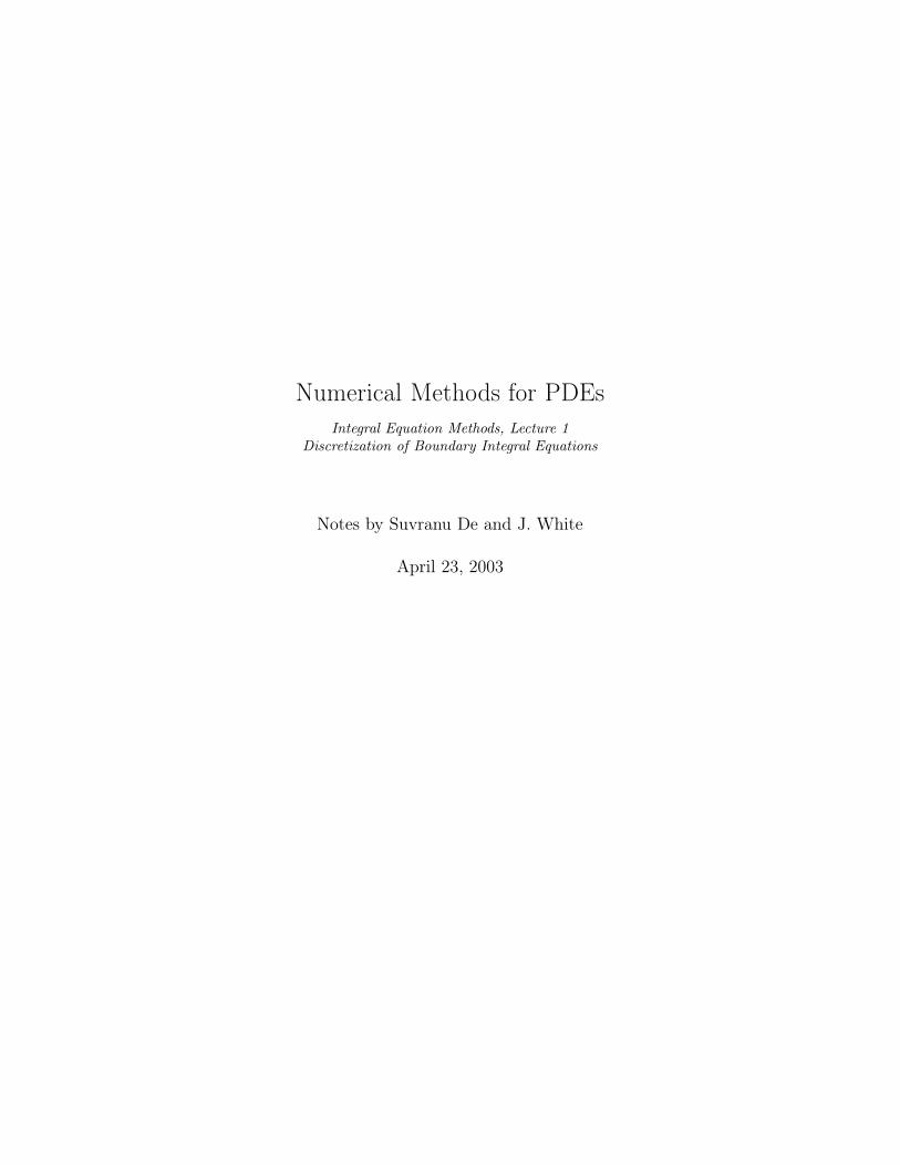
3 Interior Vs Exterior ProblemsSlide 3

Interior Exterior

Temperature known on surface

2 0T∇ =

inside

2 0T∇ =outside

Temperature known on surfac

"Temperature in a tank" "Ice cube in a bath"

What is the heat flow?Heat flow = Thermal conductivity

∫surface

∂T∂n

Note 1 Why use integral equation methods?

For both of the heat conduction examples in the above figure, the temperature,T , is a function of the spatial coordinate, x, and satisfies ∇2T (x) = 0. In both

1

problems T (x) is given on the surface, defined by Γ, and therefore both problemsare Dirichlet problems. For the “temperature in a tank” problem, the problemdomain, Ω is the interior of the cube, and for the “ice cube in a bath” problem,the problem domain is the infinitely extending region exterior to the cube. Forsuch an exterior problem, one needs an additional boundary condition to specifywhat happens sufficiently far away from the cube. Typically, it is assumed thereare no heat sources exterior to the cube and therefore

lim‖x‖→∞

T (x) → 0.

For the cube problem, we might only be interested in the net heat flow fromthe surface. That flow is given by an integral over the cube surface of thenormal derivative of temperature, scaled by a thermal conductivity. It mightseem inefficient to use the finite-element or finite-difference methods discussed inprevious sections to solve this problem, as such methods will need to computethe temperature everywhere in Ω. Indeed, it is possible to write an integralequation which relates the temperature on the surface directly to its surfacenormal, as we shall see shortly.In the four examples below, we try to demonstrate that it is quite commonin applications to have exterior problems where the known quantities and thequantities of interest are all on the surface.

4 Examples

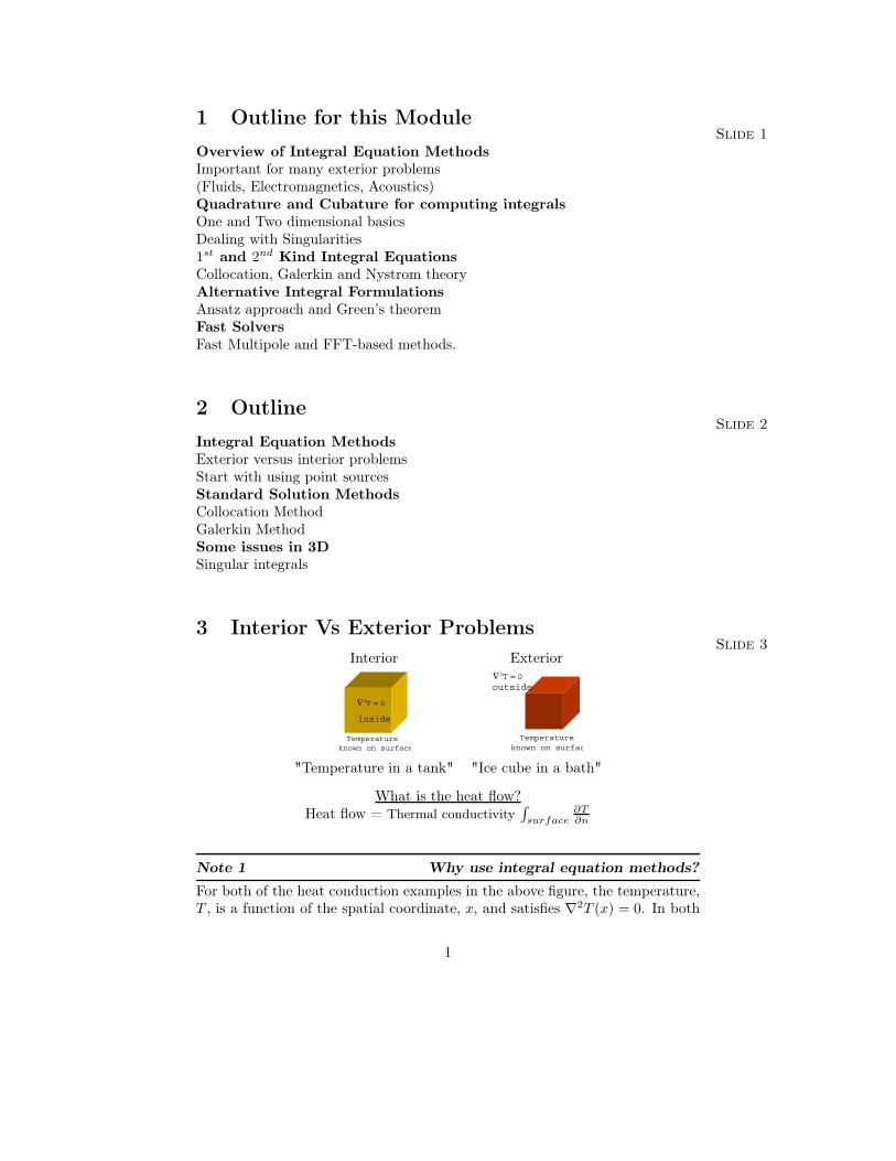
4.1 Computation of CapacitanceSlide 4

v+-2 0 Outsi∇ Ψ =

is given on SΨ

potential

What is the capacitance?Capacitance = Dielectric Permittivity

∫∂Ψ∂n

Note 2 Example 1: Capacitance problem

In the example in the slide, the yellow plates form a parallel-plate capacitorwith an applied voltage V . In this 3-D electrostatics problem, the electrostaticpotential Ψ satisfies ∇2Ψ(x) = 0 in the region exterior to the plates, and thepotential is known on the surface of the plates. In addition, far from the plates,Ψ → 0. What is of interest is the capacitance, C, which satisfies

q = CV

2

where q, the net charge on one of the plates, is given by the surface normal ofthe potential integrated over one plate and scaled by a dielectric permittivity.

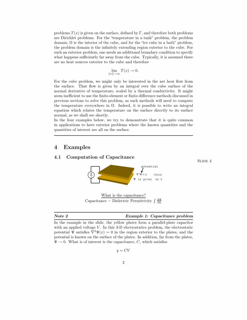
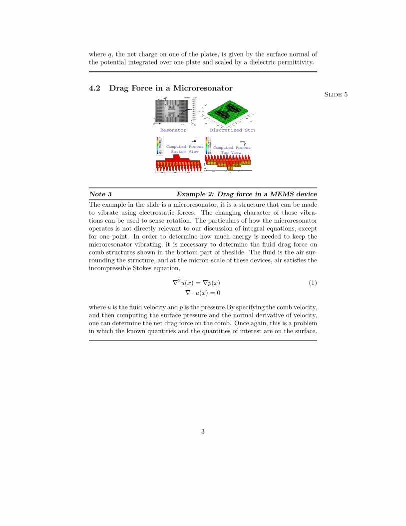
4.2 Drag Force in a MicroresonatorSlide 5

Resonator Discretized Stru

Computed ForcesBottom View

Computed ForcesTop View

Note 3 Example 2: Drag force in a MEMS device

The example in the slide is a microresonator, it is a structure that can be madeto vibrate using electrostatic forces. The changing character of those vibra-tions can be used to sense rotation. The particulars of how the microresonatoroperates is not directly relevant to our discussion of integral equations, exceptfor one point. In order to determine how much energy is needed to keep themicroresonator vibrating, it is necessary to determine the fluid drag force oncomb structures shown in the bottom part of theslide. The fluid is the air sur-rounding the structure, and at the micron-scale of these devices, air satisfies theincompressible Stokes equation,

∇2u(x) = ∇p(x) (1)∇ · u(x) = 0

where u is the fluid velocity and p is the pressure.By specifying the comb velocity,and then computing the surface pressure and the normal derivative of velocity,one can determine the net drag force on the comb. Once again, this is a problemin which the known quantities and the quantities of interest are on the surface.

3

4.3 Electromagnetic Coupling in a PackageSlide 6

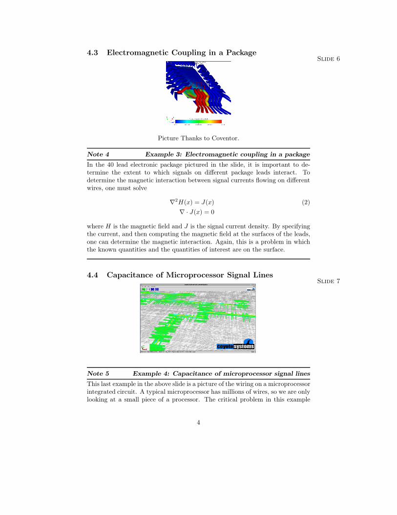
Picture Thanks to Coventor.

Note 4 Example 3: Electromagnetic coupling in a package

In the 40 lead electronic package pictured in the slide, it is important to de-termine the extent to which signals on different package leads interact. Todetermine the magnetic interaction between signal currents flowing on differentwires, one must solve

∇2H(x) = J(x) (2)∇ · J(x) = 0

where H is the magnetic field and J is the signal current density. By specifyingthe current, and then computing the magnetic field at the surfaces of the leads,one can determine the magnetic interaction. Again, this is a problem in whichthe known quantities and the quantities of interest are on the surface.

4.4 Capacitance of Microprocessor Signal LinesSlide 7

Note 5 Example 4: Capacitance of microprocessor signal lines

This last example in the above slide is a picture of the wiring on a microprocessorintegrated circuit. A typical microprocessor has millions of wires, so we are onlylooking at a small piece of a processor. The critical problem in this example

4

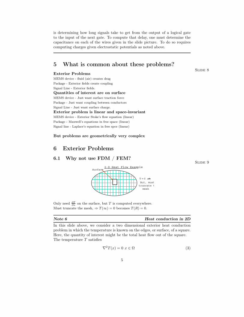
is determining how long signals take to get from the output of a logical gateto the input of the next gate. To compute that delay, one must determine thecapacitance on each of the wires given in the slide picture. To do so requirescomputing charges given electrostatic potentials as noted above.

5 What is common about these problems?Slide 8

Exterior ProblemsMEMS device - fluid (air) creates dragPackage - Exterior fields create couplingSignal Line - Exterior fields.Quantities of interest are on surfaceMEMS device - Just want surface traction forcePackage - Just want coupling between conductorsSignal Line - Just want surface charge.Exterior problem is linear and space-invariantMEMS device - Exterior Stoke’s flow equation (linear)Package - Maxwell’s equations in free space (linear)Signal line - Laplace’s equation in free spce (linear)

But problems are geometrically very complex

6 Exterior Problems

6.1 Why not use FDM / FEM?Slide 9

2-D Heat Flow Example

0 at T = ∞But, musttruncate t

mesh

Surface

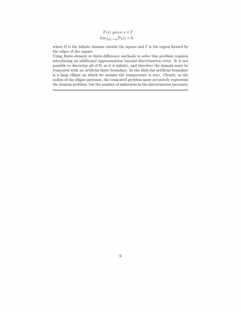
Only need ∂T∂n

on the surface, but T is computed everywhere.Must truncate the mesh, ⇒ T (∞) = 0 becomes T (R) = 0.

Note 6 Heat conduction in 2D

In this slide above, we consider a two dimensional exterior heat conductionproblem in which the temperature is known on the edges, or surface, of a square.Here, the quantity of interest might be the total heat flow out of the square.The temperature T satisfies

∇2T (x) = 0 x ∈ Ω (3)

5

T (x) given x ∈ Γlim‖x‖→∞T (x) = 0

where Ω is the infinite domain outside the square and Γ is the region formed bythe edges of the square.Using finite-element or finite-difference methods to solve this problem requiresintroducing an additional approximation beyond discretization error. It is notpossible to discretize all of Ω, as it is infinite, and therefore the domain must betruncated with an artificial finite boundary. In the slide,the artificial boundaryis a large ellipse on which we assume the temperature is zero. Clearly, as theradius of the ellipse increases, the truncated problem more accurately representsthe domain problem, but the number of unknowns in the discretization increases.

6

7 Laplace’s Equation

7.1 Green’s FunctionSlide 10

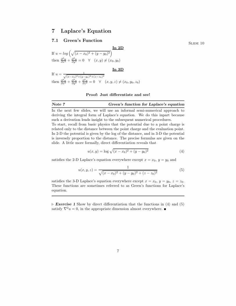
In 2DIf u = log

(√(x− x0)2 + (y − y0)2

)then ∂2u

∂x2 + ∂2u∂y2 = 0 ∀ (x, y) = (x0, y0)

In 3DIf u = 1√

(x−x0)2+(y−y0)2+(z−z0)2

then ∂2u∂x2 + ∂2u

∂y2 + ∂2u∂z2 = 0 ∀ (x, y, z) = (x0, y0, z0)

Proof: Just differentiate and see!

Note 7 Green’s function for Laplace’s equation

In the next few slides, we will use an informal semi-numerical approach toderiving the integral form of Laplace’s equation. We do this inpart becausesuch a derivation lends insight to the subsequent numerical procedures.To start, recall from basic physics that the potential due to a point charge isrelated only to the distance between the point charge and the evaluation point.In 2-D the potential is given by the log of the distance, and in 3-D the potentialis inversely proportion to the distance. The precise formulas are given on theslide. A little more formally, direct differentiation reveals that

u(x, y) = log√

(x − x0)2 + (y − y0)2 (4)

satisfies the 2-D Laplace’s equation everywhere except x = x0, y = y0 and

u(x, y, z) =1√

(x− x0)2 + (y − y0)2 + (z − z0)2(5)

satisfies the 3-D Laplace’s equation everywhere except x = x0, y = y0, z = z0.These functions are sometimes referred to as Green’s functions for Laplace’sequation.

Exercise 1 Show by direct differentiation that the functions in (4) and (5)satisfy ∇2u = 0, in the appropriate dimension almost everywhere.

7

8 Laplace’s Equation in 2D

8.1 Simple ideaSlide 11

2 2

2 2+ = 0 outs

u u

x y

∂ ∂∂ ∂

Surface

( )0 0,x y

2 2

2 2+ = 0 outside

u u

x y

∂ ∂∂ ∂

Problem Solved

is given on surfaceu

( ) ( )( )2 2

0 0Let logu x x y y= − + −

Does not match boundary conditions!

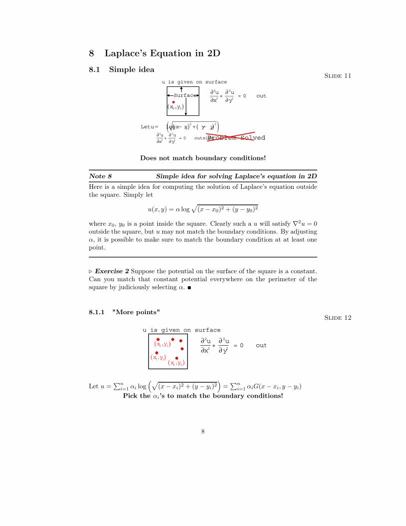
Note 8 Simple idea for solving Laplace’s equation in 2D

Here is a simple idea for computing the solution of Laplace’s equation outsidethe square. Simply let

u(x, y) = α log√

(x− x0)2 + (y − y0)2

where x0, y0 is a point inside the square. Clearly such a u will satisfy ∇2u = 0outside the square, but u may not match the boundary conditions. By adjustingα, it is possible to make sure to match the boundary condition at at least onepoint.

Exercise 2 Suppose the potential on the surface of the square is a constant.Can you match that constant potential everywhere on the perimeter of thesquare by judiciously selecting α.

8.1.1 "More points"Slide 12

2 2

2 2+ = 0 out

u u

x y

∂ ∂∂ ∂

( )1 1,x y

( )2 2,x y

is given on surfaceu

( ),n nx y

Let u =∑n

i=1 αi log(√

(x− xi)2 + (y − yi)2)

=∑n

i=1 αiG(x− xi, y − yi)Pick the αi’s to match the boundary conditions!

8

Note 9 ...contd

To construct a potential that satisfies Laplace’s equation and matches theboundary conditions at more points, let u be represented by the potential dueto a sum of n weighted point charges in the square’s interior. As shown in theslide, we can think of the potential due to a sum of charges as a sum of Green’sfunctions. Of course, we have to determine the weights on the n point charges,and the weight on the ith charge is denoted hereby αi.

8.1.2 "More points equations"Slide 13

( )1 1,x y

( )2 2,x y

( ),n nx y

( )1 1,t tx y

Source Strengths selecto give correct potent

testtestpoints.

( ) ( )

( ) ( )

( )

( )

1 1 1 1 1 11 1 1

1 1

, , ,

, , ,n n n n n n

t t t n t n t t

nt t t n t n t t

G x x y y G x x y y x y

G x x y y G x x y y x y

α

α

− − − − Ψ = − − − − Ψ

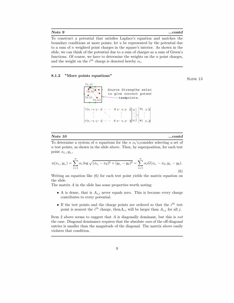
Note 10 ...contd

To determine a system of n equations for the n αi’s,consider selecting a set ofn test points, as shown in the slide above. Then, by superposition, for each testpoint xti , yti ,

u(xti , yti) =n∑i=1

αi log√

(xti − x0)2 + (yti − y0)2 =n∑i=1

αiG(xti − x0, yti − y0).(6)

Writing an equation like (6) for each test point yields the matrix equation onthe slide.The matrix A in the slide has some properties worth noting:

• A is dense, that is Ai,j never equals zero. This is because every chargecontributes to every potential.

• If the test points and the charge points are ordered so that the ith testpoint is nearest the ith charge, thenAi,i will be larger than Ai,j for all j.

Item 2 above seems to suggest that A is diagonally dominant, but this is notthe case. Diagonal dominance requires that the absolute sum of the off-diagonalentries is smaller than the magnitude of the diagonal. The matrix above easilyviolates that condition.

9

Exercise 3 Determine a set of test points and charge locations for the 2-Dsquare problem that generates anAmatrix where the magnitude of the diagonalsare bigger than the absolute value of the off-diagonals, but the magnitude ofthe diagonal is smaller than the absolute sum of the off-diagonals.

8.1.3 Computational ResultsSlide 14

R=10

rCircle with Chargesr=9.5

n=20 n=40

Potentials on the Circle

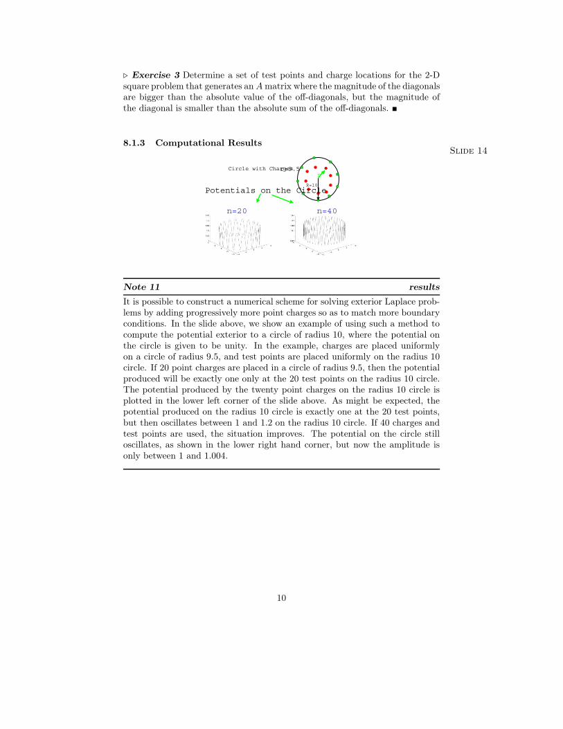
Note 11 results

It is possible to construct a numerical scheme for solving exterior Laplace prob-lems by adding progressively more point charges so as to match more boundaryconditions. In the slide above, we show an example of using such a method tocompute the potential exterior to a circle of radius 10, where the potential onthe circle is given to be unity. In the example, charges are placed uniformlyon a circle of radius 9.5, and test points are placed uniformly on the radius 10circle. If 20 point charges are placed in a circle of radius 9.5, then the potentialproduced will be exactly one only at the 20 test points on the radius 10 circle.The potential produced by the twenty point charges on the radius 10 circle isplotted in the lower left corner of the slide above. As might be expected, thepotential produced on the radius 10 circle is exactly one at the 20 test points,but then oscillates between 1 and 1.2 on the radius 10 circle. If 40 charges andtest points are used, the situation improves. The potential on the circle stilloscillates, as shown in the lower right hand corner, but now the amplitude isonly between 1 and 1.004.

10

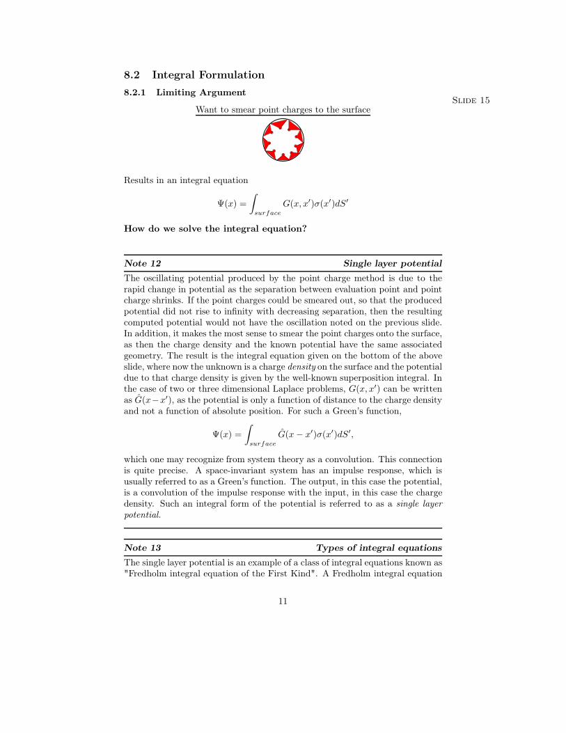
8.2 Integral Formulation8.2.1 Limiting Argument

Slide 15Want to smear point charges to the surface

Results in an integral equation

Ψ(x) =∫surface

G(x, x′)σ(x′)dS′

How do we solve the integral equation?

Note 12 Single layer potential

The oscillating potential produced by the point charge method is due to therapid change in potential as the separation between evaluation point and pointcharge shrinks. If the point charges could be smeared out, so that the producedpotential did not rise to infinity with decreasing separation, then the resultingcomputed potential would not have the oscillation noted on the previous slide.In addition, it makes the most sense to smear the point charges onto the surface,as then the charge density and the known potential have the same associatedgeometry. The result is the integral equation given on the bottom of the aboveslide, where now the unknown is a charge density on the surface and the potentialdue to that charge density is given by the well-known superposition integral. Inthe case of two or three dimensional Laplace problems, G(x, x′) can be writtenas G(x−x′), as the potential is only a function of distance to the charge densityand not a function of absolute position. For such a Green’s function,

Ψ(x) =∫surface

G(x− x′)σ(x′)dS′,

which one may recognize from system theory as a convolution. This connectionis quite precise. A space-invariant system has an impulse response, which isusually referred to as a Green’s function. The output, in this case the potential,is a convolution of the impulse response with the input, in this case the chargedensity. Such an integral form of the potential is referred to as a single layerpotential.

Note 13 Types of integral equations

The single layer potential is an example of a class of integral equations known as"Fredholm integral equation of the First Kind". A Fredholm integral equation

11

of the Second Kind results when the unknown charge density exists not onlyunder the integral sign but also outside it. An example of such an equation is

Ψ(x) = σ(x) +∫surface

K(x− x′)σ(x′)dS′,

Fredholm integral equations, in which the domain of integration is fixed, usu-ally arise out of boundary value problems. Initial value problems typically giverise to the so-called Volterra integral equations, where the domain of integra-tion depends on the output of interest. For example, consider the initial valueproblem

dx(t)dt

= tx(t); t ∈ [0, T ], T > 0.

x(t = 0) = x0

The "solution" of this equation is the following Volterra integral equation:

x(t) = x0 +∫ t

0

ξx(ξ)dξ

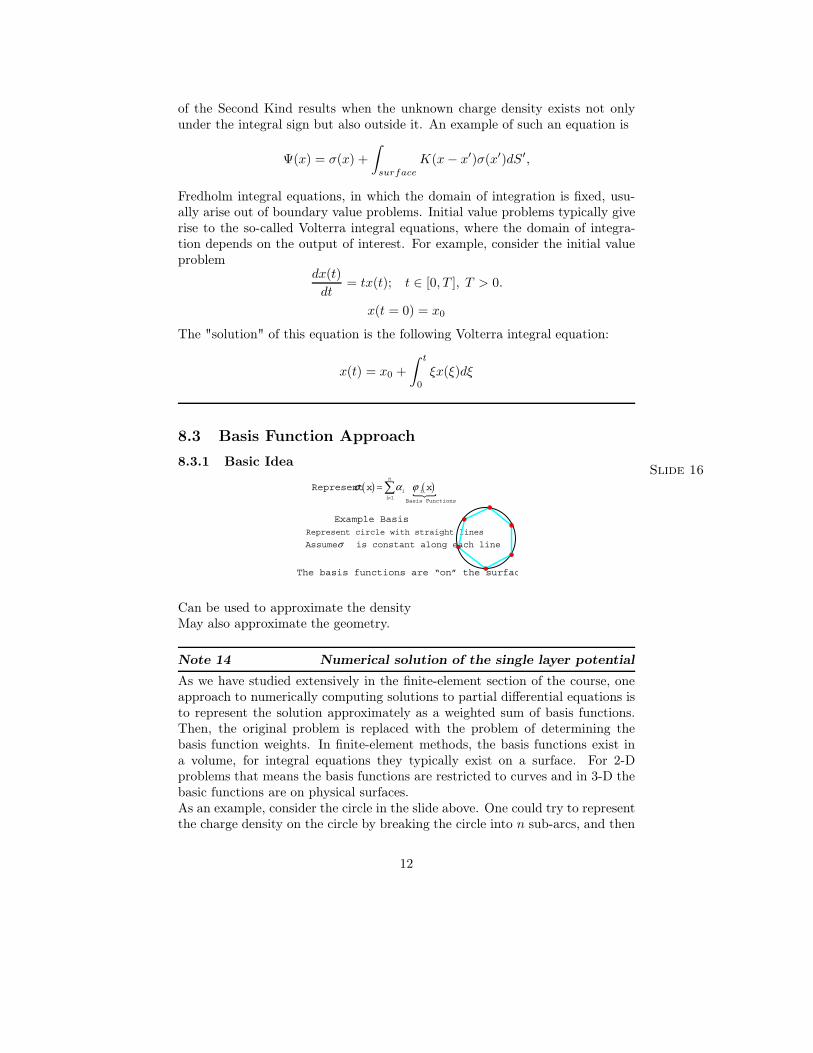
8.3 Basis Function Approach8.3.1 Basic Idea

Slide 16( ) ( )

1

Basis Functions

Represent n

i ii

x xσ α ϕ=

=

The basis functions are “on” the surfac

Example BasisRepresent circle with straight lines

Assume is constant along each lineσ

Can be used to approximate the densityMay also approximate the geometry.

Note 14 Numerical solution of the single layer potential

As we have studied extensively in the finite-element section of the course, oneapproach to numerically computing solutions to partial differential equations isto represent the solution approximately as a weighted sum of basis functions.Then, the original problem is replaced with the problem of determining thebasis function weights. In finite-element methods, the basis functions exist ina volume, for integral equations they typically exist on a surface. For 2-Dproblems that means the basis functions are restricted to curves and in 3-D thebasic functions are on physical surfaces.As an example, consider the circle in the slide above. One could try to representthe charge density on the circle by breaking the circle into n sub-arcs, and then

12

assume the charge density is a constant on each sub-arc. Such an approach is notcommonly used. Instead the geometry is usually approximated along with thecharge density. In this example case, shown in the center right of the slide, thesub-arcs of the circle are replaced with straight sections, thus forming a polygon.The charge density is assumed constant on each edge of the polygon.The resultis a piecewise constant representation of the charge density on a polygon.

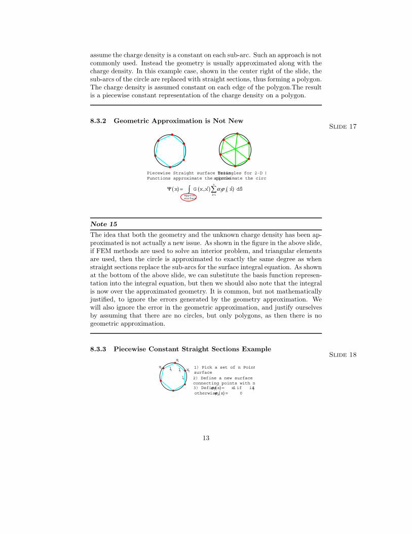
8.3.2 Geometric Approximation is Not NewSlide 17

Piecewise Straight surface basis Functions approximate the circle

Triangles for 2-D Fapproximate the circ

( ) ( ) ( )1

,n

i iiapprox

surface

x G x x x dSα ϕ=

′ ′ ′Ψ =

Note 15

The idea that both the geometry and the unknown charge density has been ap-proximated is not actually a new issue. As shown in the figure in the above slide,if FEM methods are used to solve an interior problem, and triangular elementsare used, then the circle is approximated to exactly the same degree as whenstraight sections replace the sub-arcs for the surface integral equation. As shownat the bottom of the above slide, we can substitute the basis function represen-tation into the integral equation, but then we should also note that the integralis now over the approximated geometry. It is common, but not mathematicallyjustified, to ignore the errors generated by the geometry approximation. Wewill also ignore the error in the geometric approximation, and justify ourselvesby assuming that there are no circles, but only polygons, as then there is nogeometric approximation.

8.3.3 Piecewise Constant Straight Sections ExampleSlide 18

1) Pick a set of n Pointsurface

1x

2) Define a new surface connecting points with n

( )i3) Define 1 if is ix x lϕ =( )iotherwise, 0 xϕ =

2xnx

1l

2l

nl

13

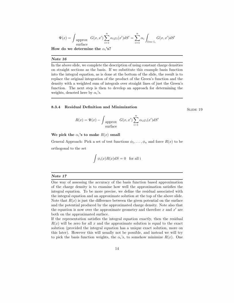
Ψ(x) =∫

approxsurface

G(x, x′)n∑i=1

αiϕi(x′)dS′ =n∑i=1

αi

∫line li

G(x, x′)dS′

How do we determine the αi’s?

Note 16

In the above slide, we complete the description of using constant charge densitieson straight sections as the basis. If we substitute this example basis functioninto the integral equation, as is done at the bottom of the slide, the result is toreplace the original integration of the product of the Green’s function and thedensity with a weighted sum of integrals over straight lines of just the Green’sfunction. The next step is then to develop an approach for determining theweights, denoted here by αi’s.

8.3.4 Residual Definition and MinimizationSlide 19

R(x) = Ψ(x) −∫

approxsurface

G(x, x′)n∑i=1

αiϕi(x′)dS′

We pick the αi’s to make R(x) small

General Approach: Pick a set of test functions φ1, . . . , φn and force R(x) to be

orthogonal to the set ∫φi(x)R(x)dS = 0 for all i

Note 17

One way of assessing the accuracy of the basis function based approximationof the charge density is to examine how well the approximation satisfies theintegral equation. To be more precise, we define the residual associated withthe integral equation and an approximate solution at the top of the above slide.Note that R(x) is just the difference between the given potential on the surfaceand the potential produced by the approximated charge density. Note also thatthe equation is now over the approximate geometry and therefore x and x′ areboth on the approximated surface.If the representation satisfies the integral equation exactly, then the residualR(x) will be zero for all x and the approximate solution is equal to the exactsolution (provided the integral equation has a unique exact solution, more onthis later). However this will usually not be possible, and instead we will tryto pick the basis function weights, the αi’s, to somehow minimize R(x). One

14

approach to minimizing R(x) is to make it orthogonal to a collection of testfunctions, which may or may not be related to the basis functions. As notedon the bottom of the slide, enforcing orthogonality in this case means ensuringthat the integral of the product of R(x) and φ(x) over the surface is zero.

15

8.3.5 Residual Minimization Using Test FunctionsSlide 20∫

φi(x)R(x)dS = 0 ⇒∫φi(x)Ψ(x)dS −

∫ ∫approxsurface

φi(x)G(x, x′)n∑j=1

αjϕj(x′)dS′dS = 0

We will generate different methods by choosing the φ1, . . . , φn

Collocation : φi(x) = δ(x − xti) (point matching)Galerkin Method : φi(x) = ϕi(x) (basis = test)Weighted Residual Method : φi(x) = 1 if ϕi(x) = 0 (averages)

Note 18

As noted in the equation on the top of the above slide, by substituting thedefinition of the residual into the orthogonality equation given in the previousslide, it is possible to generate n equations, one for each test function. Thegenerated equation has two integrals. The first is a surface integral of theproduct of the given potential with the test function. The second integral isa double integral over the surface. The integrand of the double integral isa product of the test function, the Green’s function, and the charge densityrepresentation.As noted in the slide, and as we will describe in more detail below, three differentnumerical techniques can be derived by altering the test functions.

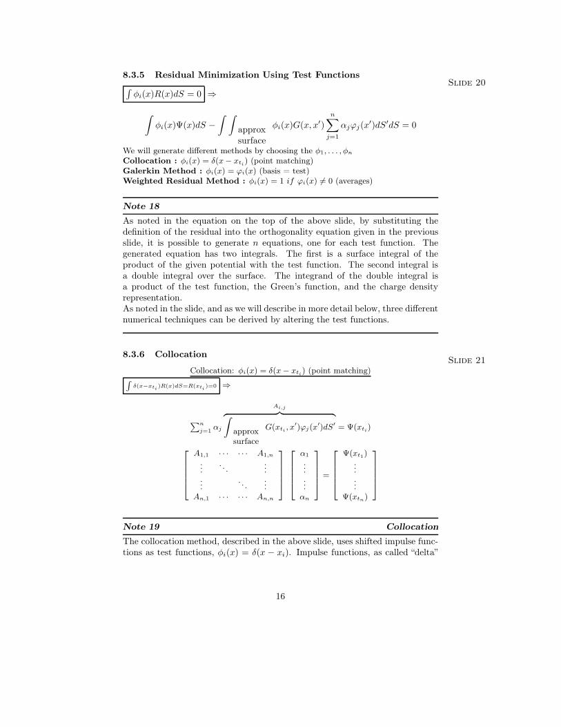
8.3.6 CollocationSlide 21

Collocation: φi(x) = δ(x − xti) (point matching)∫δ(x−xti

)R(x)dS=R(xti)=0 ⇒

∑n

j=1αj

Ai,j︷ ︸︸ ︷∫approxsurface

G(xti , x′)ϕj(x

′)dS′ = Ψ(xti)

A1,1 · · · · · · A1,n

.... . .

......

. . ....

An,1 · · · · · · An,n

α1

...

...αn

=

Ψ(xt1)......

Ψ(xtn)

Note 19 Collocation

The collocation method, described in the above slide, uses shifted impulse func-tions as test functions, φi(x) = δ(x − xi). Impulse functions, as called “delta”

16

functions, have a sifting property when integrated with a smooth function f(x),∫f(x)δ(x − xi)dx = f(xi).

Impulse functions are also referred to as generalized functions, and they arespecified only by their behavior when integrated with a smooth function. In thecase of the impulse function, one can think of the function as being zero exceptfor a very narrow interval around xi, and then being so large in that narrowinterval that

∫δ(x− xi)dx = 1.

As the summation equation in the middle of the above slide indicates, testingwith impulse functions is equivalent to insisting that R(xi) = 0, or in words,that the potential produced by the approximated charge density should matchthe given potential at n test points. That the potentials match at the testpoints gives rise to the method’s name, the point where the potential is exactlymatched is “co-located” with a set of test points.The n × n matrix equation at the bottom of the above slide has as its right-hand side the potentials at the test points. The unknowns are the basis functionweights. The jth matrix element for the ith row is the potential produced attest point xi by a charge density equal to basis function ϕj .

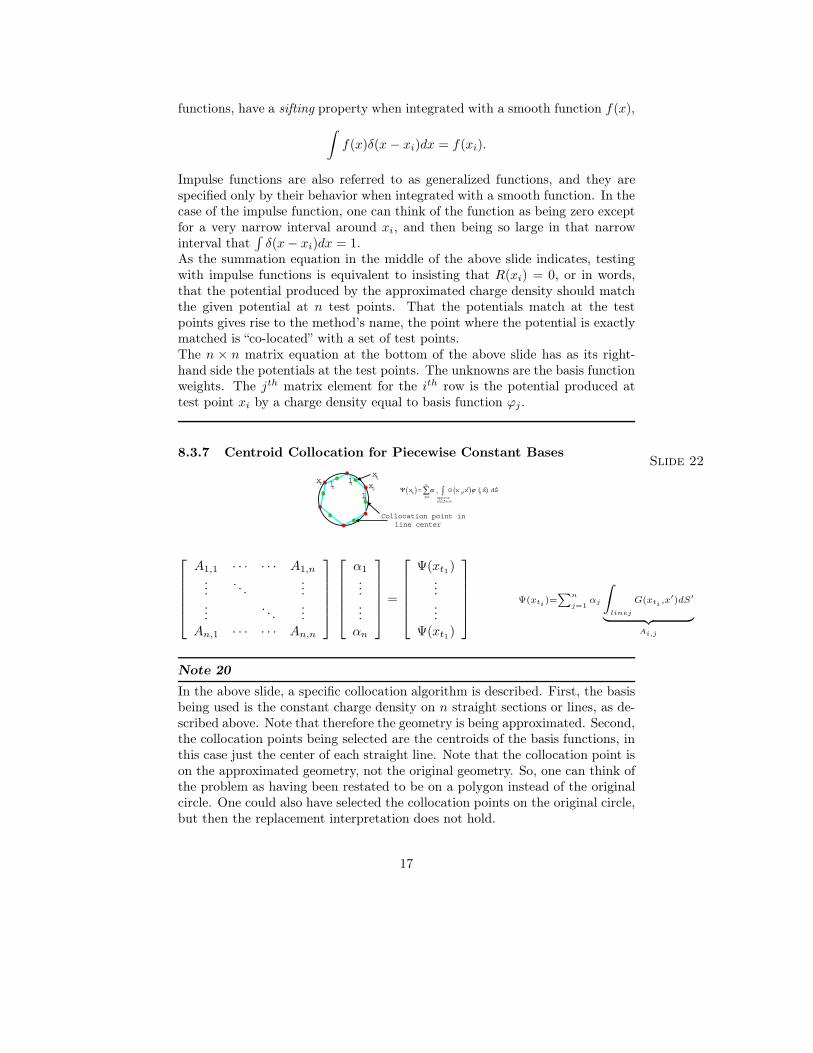
8.3.7 Centroid Collocation for Piecewise Constant BasesSlide 22

( ) ( ) ( )1

,i i

n

t j t jj approx

surface

x G x x x dSα ϕ=

′ ′ ′Ψ = 2xnx 1l

2lnl

Collocation point in line center

1tx

A1,1 · · · · · · A1,n

.... . .

......

. . ....

An,1 · · · · · · An,n

α1

...

...αn

=

Ψ(xt1)......

Ψ(xt1)

Ψ(xti

)=∑

n

j=1αj

∫linej

G(xti,x′)dS′

︸ ︷︷ ︸Ai,j

Note 20

In the above slide, a specific collocation algorithm is described. First, the basisbeing used is the constant charge density on n straight sections or lines, as de-scribed above. Note that therefore the geometry is being approximated. Second,the collocation points being selected are the centroids of the basis functions, inthis case just the center of each straight line. Note that the collocation point ison the approximated geometry, not the original geometry. So, one can think ofthe problem as having been restated to be on a polygon instead of the originalcircle. One could also have selected the collocation points on the original circle,but then the replacement interpretation does not hold.

17

In collocation, or point- matching, the charge densities on each of the straightlines are selected so that the resulting potential at the line centers matches thegiven potential. As the equations on this slide make clear, the matrix elementAi,j is the potential at the center of line i due to a unit charge density alongline j.It should be noted that the matrix A is dense, the charge on line j contributesto the potential everywhere. Also note that if line j is far away from line i, then

Ai,j ≈ length(linej) ∗G(xti , xtj ) (7)

Exercise 4 Suppose we are using piecewise constant centroid collocationto solve a 2-D Laplace problem, so G(x, y, x′, y′) = log

√(x− x′)2 + (y − y′)2.

Roughly how far apart do line sections i and j have to be for (7) to be accurate towithin one percent? Assume line j has length of one. Does your answer dependon the orientation of line j? Does your answer depend on the orientation of linei? (You should answer yes to one of these and no to the other, do you see why?)

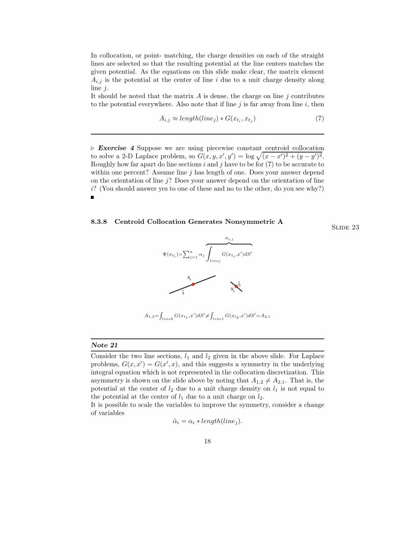
8.3.8 Centroid Collocation Generates Nonsymmetric ASlide 23

Ψ(xti)=

∑n

j=1αj

Ai,j︷ ︸︸ ︷∫linej

G(xti,x′)dS′

1l

2l1tx

2tx

A1,2=∫

line2G(xt1 ,x

′)dS′ =∫

line1G(xt2 ,x

′)dS′=A2,1

Note 21

Consider the two line sections, l1 and l2 given in the above slide. For Laplaceproblems, G(x, x′) = G(x′, x), and this suggests a symmetry in the underlyingintegral equation which is not represented in the collocation discretization. Thisasymmetry is shown on the slide above by noting that A1,2 = A2,1. That is, thepotential at the center of l2 due to a unit charge density on l1 is not equal tothe potential at the center of l1 due to a unit charge on l2.It is possible to scale the variables to improve the symmetry, consider a changeof variables

αi = αi ∗ length(linej).

18

In this change of variables, the unknowns αi are now the net line charges ratherthan the line charge densities. In this new system, Aα = Ψ, where the elementsof the matrix A are given by

Ai,j =1

length(linej)

∫linej

G(xti , x′)dS′.

Under the change of variables, if line j is far away from line i, then

Ai,j ≈ G(xti , xtj ) ≈ Aj,i. (8)

In other words, the elements of A corresponding to distant terms are approxi-mately symmetric.

Exercise 5 Give an example which shows that the scaled entries of A can befar from symmetric. Assume we are using piecewise constant straight sectionswith centroid collocation and the 2-D Laplace’s equation Green’s function.

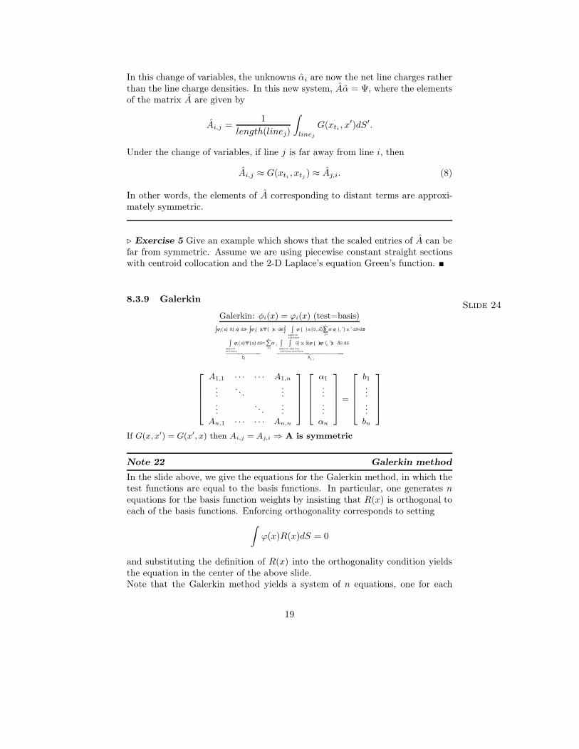
8.3.9 GalerkinSlide 24

Galerkin: φi(x) = ϕi(x) (test=basis)( ) ( ) ( ) ( ) ( ) ( ) ( )

1

, 0n

i i i j jjapprox

surface

x R x dS x x dS x G x x x dS dSϕ ϕ ϕ α ϕ=

′ ′ ′= Ψ − =

( ) ( ) ( ) ( ) ( )1

,

,n

i j i jjapprox approx approx

surface surface surface

i ji

x x dS G x x x x dS dS

Ab

ϕ α ϕ ϕ=

′ ′ ′Ψ =

A1,1 · · · · · · A1,n

.... . .

......

. . ....

An,1 · · · · · · An,n

α1

...

...αn

=

b1

...

...bn

If G(x, x′) = G(x′, x) then Ai,j = Aj,i ⇒ A is symmetric

Note 22 Galerkin method

In the slide above, we give the equations for the Galerkin method, in which thetest functions are equal to the basis functions. In particular, one generates nequations for the basis function weights by insisting that R(x) is orthogonal toeach of the basis functions. Enforcing orthogonality corresponds to setting

∫ϕ(x)R(x)dS = 0

and substituting the definition of R(x) into the orthogonality condition yieldsthe equation in the center of the above slide.Note that the Galerkin method yields a system of n equations, one for each

19

orthogonality condition, and n unknowns, one for each basis function weight.Also, the system does not have the potential explicitly as the right hand side.Instead, the ith right- hand side entry is the average of the product of thepotential and the ith basis function.

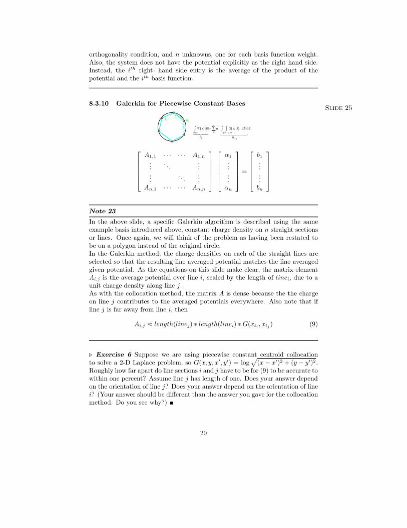
8.3.10 Galerkin for Piecewise Constant BasesSlide 25

2xnx1l

2lnl

( ) ( )1

,

,i i j

n

jjline line line

i i j

x dS G x x dS dS

b A

α=

′ ′Ψ =

A1,1 · · · · · · A1,n

.... . .

......

. . ....

An,1 · · · · · · An,n

α1

...

...αn

=

b1......bn

Note 23

In the above slide, a specific Galerkin algorithm is described using the sameexample basis introduced above, constant charge density on n straight sectionsor lines. Once again, we will think of the problem as having been restated tobe on a polygon instead of the original circle.In the Galerkin method, the charge densities on each of the straight lines areselected so that the resulting line averaged potential matches the line averagedgiven potential. As the equations on this slide make clear, the matrix elementAi,j is the average potential over line i, scaled by the length of linei, due to aunit charge density along line j.As with the collocation method, the matrix A is dense because the the chargeon line j contributes to the averaged potentials everywhere. Also note that ifline j is far away from line i, then

Ai,j ≈ length(linej) ∗ length(linei) ∗G(xti , xtj ) (9)

Exercise 6 Suppose we are using piecewise constant centroid collocationto solve a 2-D Laplace problem, so G(x, y, x′, y′) = log

√(x− x′)2 + (y − y′)2.

Roughly how far apart do line sections i and j have to be for (9) to be accurate towithin one percent? Assume line j has length of one. Does your answer dependon the orientation of line j? Does your answer depend on the orientation of linei? (Your answer should be different than the answer you gave for the collocationmethod. Do you see why?)

20

9 Laplace’s Equation in 3D

9.1 Electrostatics Example9.1.1 Dirichlet Problem

Slide 26

v+-2 0 Outsi∇ Ψ =

is given on SΨ

potential

First kind integral equation for charge:

Ψ(x)︸ ︷︷ ︸Potential

=∫surface

1||x− x′||︸ ︷︷ ︸

Green′s function

σ(x′)︸ ︷︷ ︸Charge density

dS′

Note 24

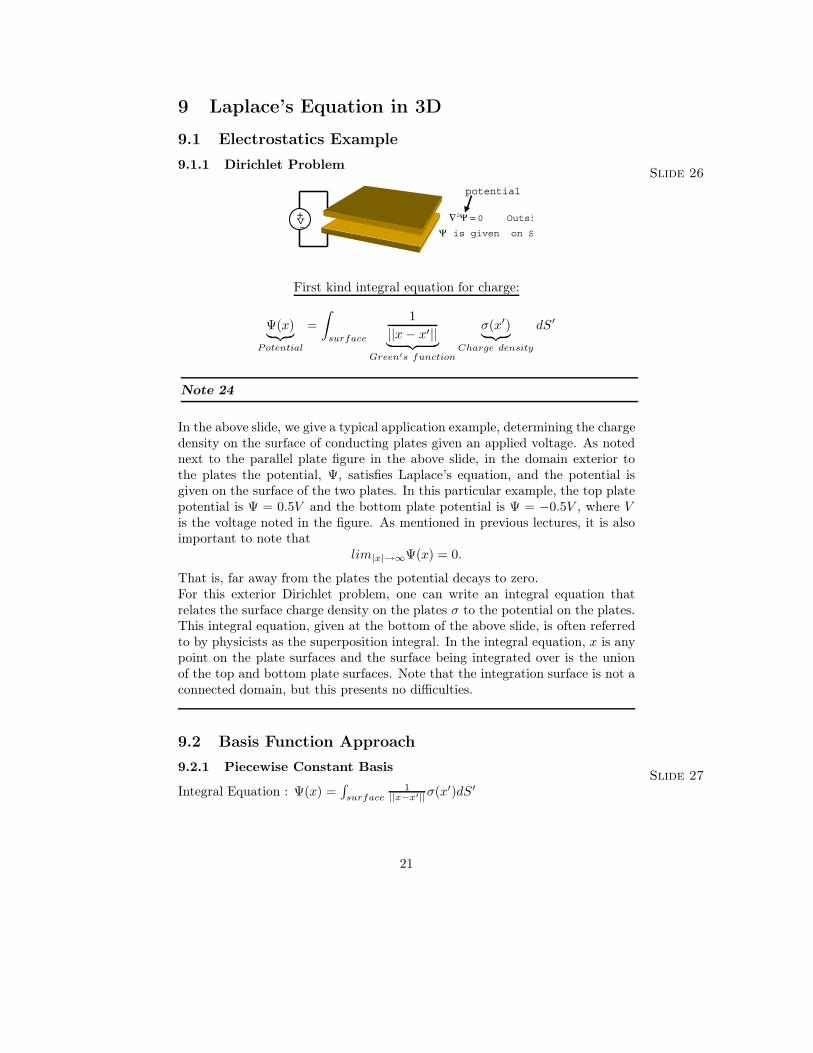
In the above slide, we give a typical application example, determining the chargedensity on the surface of conducting plates given an applied voltage. As notednext to the parallel plate figure in the above slide, in the domain exterior tothe plates the potential, Ψ, satisfies Laplace’s equation, and the potential isgiven on the surface of the two plates. In this particular example, the top platepotential is Ψ = 0.5V and the bottom plate potential is Ψ = −0.5V , where Vis the voltage noted in the figure. As mentioned in previous lectures, it is alsoimportant to note that

lim|x|→∞Ψ(x) = 0.

That is, far away from the plates the potential decays to zero.For this exterior Dirichlet problem, one can write an integral equation thatrelates the surface charge density on the plates σ to the potential on the plates.This integral equation, given at the bottom of the above slide, is often referredto by physicists as the superposition integral. In the integral equation, x is anypoint on the plate surfaces and the surface being integrated over is the unionof the top and bottom plate surfaces. Note that the integration surface is not aconnected domain, but this presents no difficulties.

9.2 Basis Function Approach9.2.1 Piecewise Constant Basis

Slide 27Integral Equation : Ψ(x) =

∫surface

1||x−x′||σ(x

′)dS′

21

( ) 1 if is on j x xϕ =( ) 0 otherwisej xϕ =

Discretize Surface into Panels

Panel j

( ) ( )

1Basis Functio

Represent n

i ii

x xσ α ϕ=

≈

Note 25

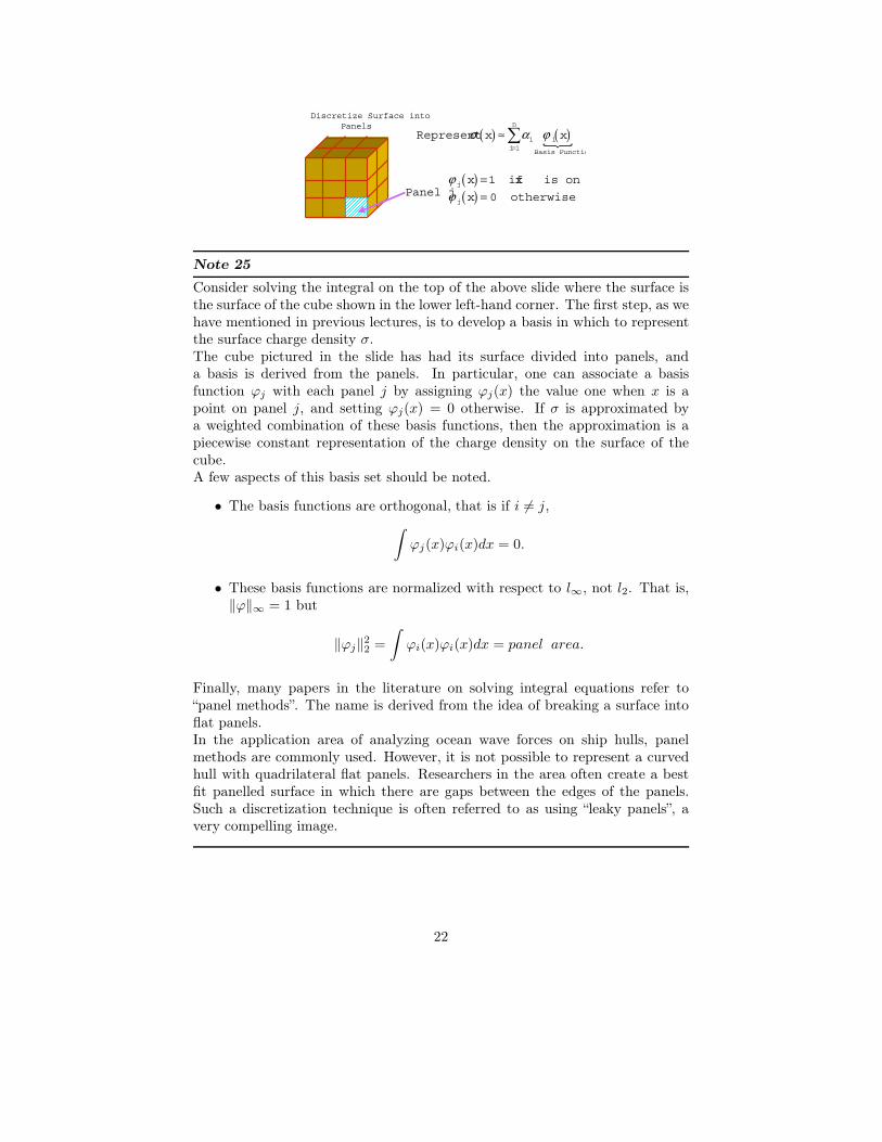
Consider solving the integral on the top of the above slide where the surface isthe surface of the cube shown in the lower left-hand corner. The first step, as wehave mentioned in previous lectures, is to develop a basis in which to representthe surface charge density σ.The cube pictured in the slide has had its surface divided into panels, anda basis is derived from the panels. In particular, one can associate a basisfunction ϕj with each panel j by assigning ϕj(x) the value one when x is apoint on panel j, and setting ϕj(x) = 0 otherwise. If σ is approximated bya weighted combination of these basis functions, then the approximation is apiecewise constant representation of the charge density on the surface of thecube.A few aspects of this basis set should be noted.

• The basis functions are orthogonal, that is if i = j,∫ϕj(x)ϕi(x)dx = 0.

• These basis functions are normalized with respect to l∞, not l2. That is,‖ϕ‖∞ = 1 but

‖ϕj‖22 =

∫ϕi(x)ϕi(x)dx = panel area.

Finally, many papers in the literature on solving integral equations refer to“panel methods”. The name is derived from the idea of breaking a surface intoflat panels.In the application area of analyzing ocean wave forces on ship hulls, panelmethods are commonly used. However, it is not possible to represent a curvedhull with quadrilateral flat panels. Researchers in the area often create a bestfit panelled surface in which there are gaps between the edges of the panels.Such a discretization technique is often referred to as using “leaky panels”, avery compelling image.

22

9.2.2 Centroid CollocationSlide 28

Put collocation points at panel centroids

( )1

,

1i

i

n

c jj c

i j

panel j

x dSx x

A

α=

′Ψ =′−

( )

( )

11,1 1, 1

,1 ,n

cn

n n n n c

xA A

A A x

α

α

Ψ = Ψ

icx Collocation

point

Note 26

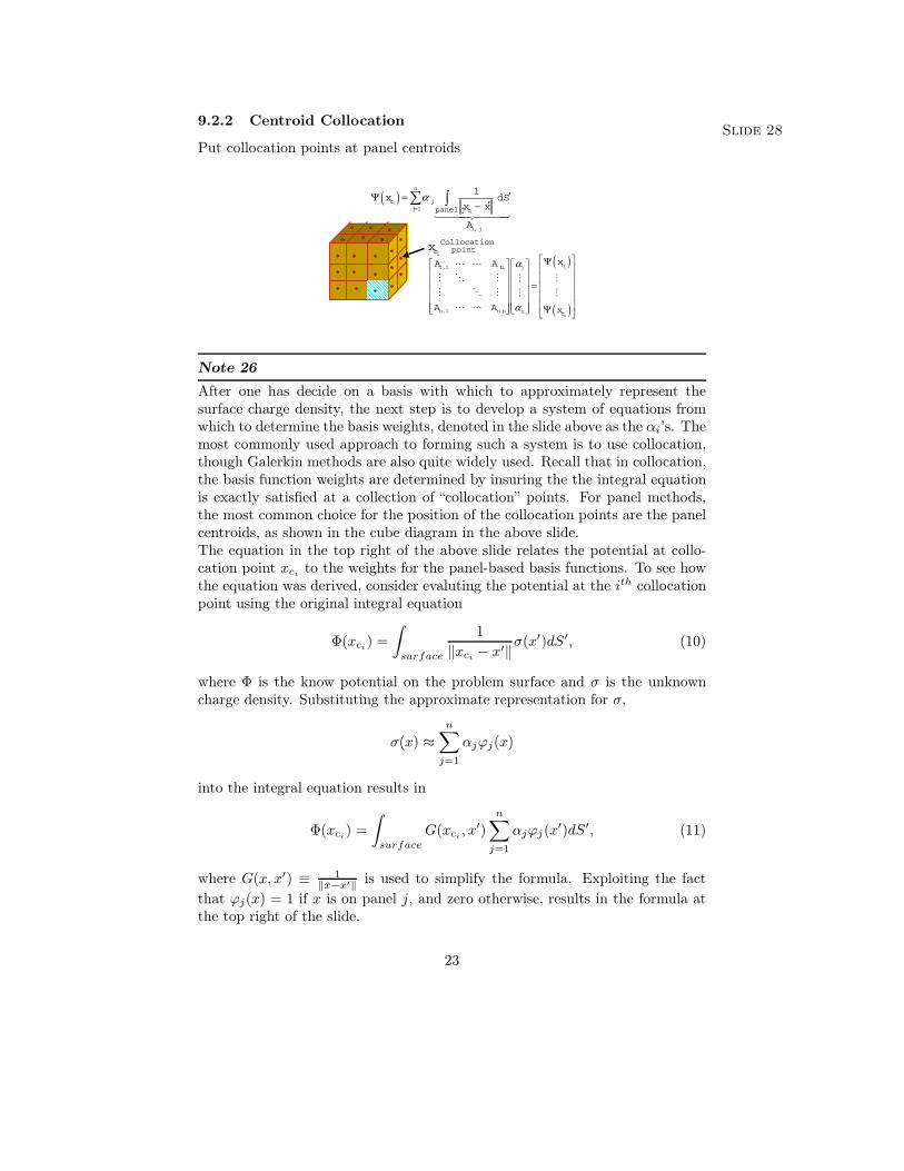
After one has decide on a basis with which to approximately represent thesurface charge density, the next step is to develop a system of equations fromwhich to determine the basis weights, denoted in the slide above as the αi’s. Themost commonly used approach to forming such a system is to use collocation,though Galerkin methods are also quite widely used. Recall that in collocation,the basis function weights are determined by insuring the the integral equationis exactly satisfied at a collection of “collocation” points. For panel methods,the most common choice for the position of the collocation points are the panelcentroids, as shown in the cube diagram in the above slide.The equation in the top right of the above slide relates the potential at collo-cation point xci to the weights for the panel-based basis functions. To see howthe equation was derived, consider evaluting the potential at the ith collocationpoint using the original integral equation

Φ(xci) =∫surface

1‖xci − x′‖

σ(x′)dS′, (10)

where Φ is the know potential on the problem surface and σ is the unknowncharge density. Substituting the approximate representation for σ,

σ(x) ≈n∑j=1

αjϕj(x)

into the integral equation results in

Φ(xci) =∫surface

G(xci , x′)

n∑j=1

αjϕj(x′)dS′, (11)

where G(x, x′) ≡ 1‖x−x′‖ is used to simplify the formula. Exploiting the fact

that ϕj(x) = 1 if x is on panel j, and zero otherwise, results in the formula atthe top right of the slide.

23

The system of equations from which to determine the basis function weights isgiven in the lower right corner of the slide. The right hand side of the systemis the vector of known potentials at the collocation points. The i, jth elementof the matrix A is the potential produced at collocation point i due to a unitcharge density on panel j. The vector of α’s are the unknown panel chargedensities.

Exercise 7 Determine a scaling of the α’s (αi = ciαi) such that the scaledmatrix A has the property

Ai,j ≈ 1‖xci − xcj‖

when ‖xci − xcj‖ is much larger than a panel diameter.

9.2.3 Calculating Matrix ElementsSlide 29

Panel j

icx Collocation

point

,

1

i

i j

pa cnel j x xA dS′

′−=

,

i jc centr

j

id

i

o

Panel Area

x xA

−≈One point

quadratureApproximation

x

yz

t

4

,1 in

0.25*

i jc o

i jj p

Ar a

x xA

e

= −≈ Four point

quadratureApproximation

Note 27

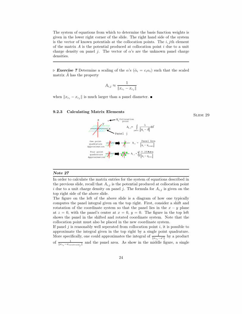
In order to calculate the matrix entries for the system of equations described inthe previous slide, recall that Ai,j is the potential produced at collocation pointi due to a unit charge density on panel j. The formula for Ai,j is given on thetop right side of the above slide.The figure on the left of the above slide is a diagram of how one typicallycomputes the panel integral given on the top right. First, consider a shift androtatation of the coordinate system so that the panel lies in the x − y planeat z = 0, with the panel’s center at x = 0, y = 0. The figure in the top leftshows the panel in the shifted and rotated coordinate system. Note that thecollocation point must also be placed in the new coordinate system.If panel j is reasonably well seperated from collocation point i, it is possible toapproximate the integral given in the top right by a single point quadrature.More specifically, one could approximates the integral of 1

‖xci−x′‖ by a product

of 1‖xci

−xcentroidj‖ and the panel area. As show in the middle figure, a single

24

point quadrature is like treating the panel as if it were a point charge at thepanel’s centroid, where the point charge’s strength is equal to the panel area.If the collocation point is close to the panel, then a single point quadraturewill be insufficiently accurate. Instead, a more accurate four point quadraturescheme would be to break the panel into four subpanels, and then treat each ofthe subpanels as point charges at their respective centers. This simple idea isshown in the figure at the bottom of the above slide. This four point scheme isequivalent to ∫

panelj

1‖xci − x′‖

dS′ ≈4∑

j=1

0.25 ∗Area‖xci − xpointj ‖

.

If the panel is a unit square in the x-y plane whose center is at the coordinatesystem origin, then the four xpointj ’s are (x, y, z) = (0.25, 0.25, 0), (x, y, z) =(−0.25, 0.25, 0), (x, y, z) = (−0.25,−0.25, 0), and (x, y, z) = (0.25,−0.25, 0).

9.2.4 Calculating "Self Term"Slide 30

Panel i

icx Collocation

point

,

0

i i

i i

c c

Panel AreaA

x x−≈

One point quadrature

Approximation

x

yz

, is an integrable sin1

i

i i

panel i cx xA dS

′−′=

,

1

i

i i

pa cnel i x xA dS′

′−=

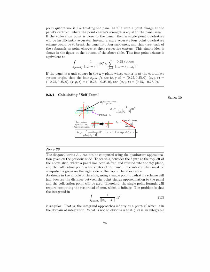
Note 28

The diagonal terms Ai,i can not be computed using the quadrature approxima-tion given on the previous slide. To see this, consider the figure at the top left ofthe above slide, where a panel has been shifted and rotated into the x-y plane,and the collocation point is the center of the panel. The integral that must becomputed is given on the right side of the top of the above slide.As shown in the middle of the slide, using a single point quadrature scheme willfail, because the distance between the point charge approximation to the paneland the collocation point will be zero. Therefore, the single point formula willrequire computing the reciprocal of zero, which is infinite. The problem is thatthe integrand in ∫

paneli

1‖xci − x′‖

dS′ (12)

is singular. That is, the integrand approaches infinity at a point x′ which is inthe domain of integration. What is not so obvious is that (12) is an integrable

25

singularity. Therefore, even though the integrand approaches infinity at somepoint, the “area under the curve” is finite.

9.2.5 Calculating "Self Term"Tricks of the Trade

Slide 31

Panel i

icx Collocation

point

,

1

i

i i

pa cnel i x xA dS′

′−= x

yz

Disk of radius R surrounding

collocation point

,

1 1

i ic c

i i

disk rest of panel

A dS dSx x x x′ ′− −

′ ′= +

Disk Integral has singularity but has analytic formula

Integrate in two pieces

2

0 0

12

1

i

R

d k cis

dS rdrd Rrx x

π

θ π′

′ = =−

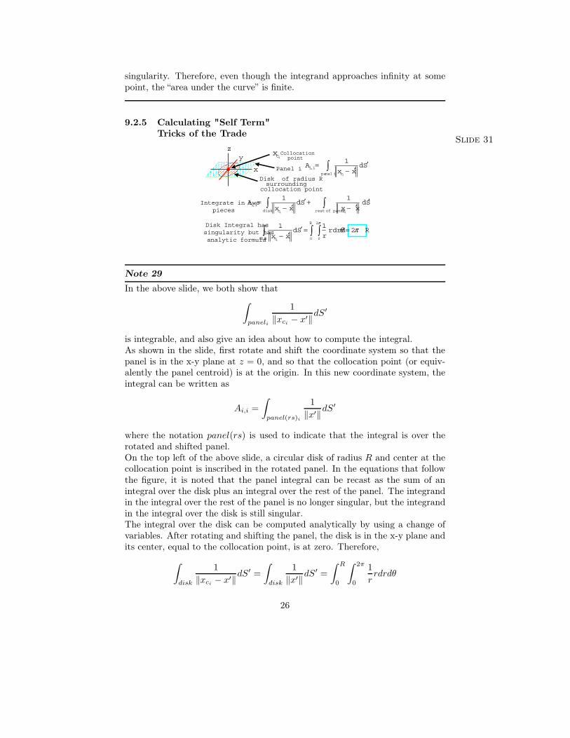
Note 29

In the above slide, we both show that∫paneli

1‖xci − x′‖

dS′

is integrable, and also give an idea about how to compute the integral.As shown in the slide, first rotate and shift the coordinate system so that thepanel is in the x-y plane at z = 0, and so that the collocation point (or equiv-alently the panel centroid) is at the origin. In this new coordinate system, theintegral can be written as

Ai,i =∫panel(rs)i

1‖x′‖dS

′

where the notation panel(rs) is used to indicate that the integral is over therotated and shifted panel.On the top left of the above slide, a circular disk of radius R and center at thecollocation point is inscribed in the rotated panel. In the equations that followthe figure, it is noted that the panel integral can be recast as the sum of anintegral over the disk plus an integral over the rest of the panel. The integrandin the integral over the rest of the panel is no longer singular, but the integrandin the integral over the disk is still singular.The integral over the disk can be computed analytically by using a change ofvariables. After rotating and shifting the panel, the disk is in the x-y plane andits center, equal to the collocation point, is at zero. Therefore,

∫disk

1‖xci − x′‖

dS′ =∫disk

1‖x′‖dS

′ =∫ R

0

∫ 2π

0

1rrdrdθ

26

where r =√x2 + y2, rsinθ = x and rcosθ = y. As given in the bottom of the

above slide, the integral over the disk is 2πR.

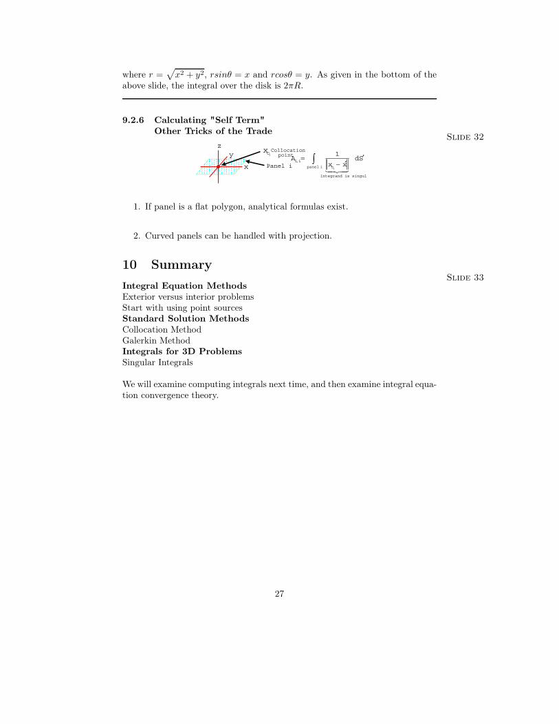
9.2.6 Calculating "Self Term"Other Tricks of the Trade

Slide 32

Panel i

icx Collocation

point

Integrand is singul

,

1

i

i i

panel i cx xA dS

′′=

−x

yz

1. If panel is a flat polygon, analytical formulas exist.

2. Curved panels can be handled with projection.

10 SummarySlide 33

Integral Equation MethodsExterior versus interior problemsStart with using point sourcesStandard Solution MethodsCollocation MethodGalerkin MethodIntegrals for 3D ProblemsSingular Integrals

We will examine computing integrals next time, and then examine integral equa-tion convergence theory.

27