numerical metho numerical methods cal methods
TRANSCRIPT
NUMERICAL METHODS
VI SEMESTER
CORE COURSE
B Sc MATHEMATICS
(2011 Admission)
UNIVERSITY OF CALICUTSCHOOL OF DISTANCE EDUCATION
Calicut university P.O, Malappuram Kerala, India 673 635.
359
NUMERICAL METHODS
VI SEMESTER
CORE COURSE
B Sc MATHEMATICS
(2011 Admission)
UNIVERSITY OF CALICUTSCHOOL OF DISTANCE EDUCATION
Calicut university P.O, Malappuram Kerala, India 673 635.
359
NUMERICAL METHODS
VI SEMESTER
CORE COURSE
B Sc MATHEMATICS
(2011 Admission)
UNIVERSITY OF CALICUTSCHOOL OF DISTANCE EDUCATION
Calicut university P.O, Malappuram Kerala, India 673 635.
359
School of Distance Education
Numerical Methods Page 2
UNIVERSITY OF CALICUTSCHOOL OF DISTANCE EDUCATIONSTUDY MATERIAL
Core Course
B Sc Mathematics
VI Semester
NUMERICAL METHODS
Prepared by: Sri.Nandakumar M.,Assistant ProfessorDept. of Mathematics,N.A.M. College, Kal likkandy.Kannur.
Scrutinized by: Dr. V. Anil Kumar,Reader,Dept. of Mathematics,University of Calicut.
Layout: Computer Section, SDE
©Reserved
School of Distance Education
Numerical Methods Page 3
Contents Page No.
MODULE I
1 Fixed Point Iteration Method 6
2 Bisection and Regula False Methods 18
3 Newton Raphson Method etc. 32
4 Finite Differences Operators 51
MODULE II
5 Numerical Interpolation 71
6 Newton’s and Lagrangian Formulae– Part I 87
7 Newton’s and Lagrangian Formulae– Part II 100
8 Interpolation by Iteration 114
9 Numerical Differentiaton 119
10 Numerical Integration 128
MODULE III
11 Solution of System of LinearEquations 140
12 Solution by Iterations 161
13 Eigen Values 169
MODULE IV
14 Taylor Series Method 179
15 Picard’s Iteration Method 187
16 Euler Methods 195
17 Runge – Kutta Methods 203
18 Predictor and Corrector Methods 214
School of Distance Education
Numerical Methods Page 4
SYLLABUS
B.Sc. DEGREE PROGRAMME
MATHEMATICS
MM6B11 : NUMERICAL METHODS
4 credits 30 weightage
Text :
S.S. Sastry : Introductory Methods of Numerical Analysis, Fourth Edition, PHI.
Module I : Solution of Algebraic and Transcendental Equation
2.1 Introduction
2.2 Bisection Method
2.3 Method of false position
2.4 Iteration method
2.5 Newton-Raphson Method
2.6 Ramanujan's method
2.7 The Secant Method
Finite Differences
3.1 Introduction
3.3.1 Forward differences
3.3.2 Backward differences
3.3.3 Central differences
3.3.4 Symbolic relations and separation of symbols
3.5 Differences of a polynomial
Module II : Interpolation
3.6 Newton's formulae for intrapolation
3.7 Central difference interpolation formulae
3.7.1 Gauss' Central Difference Formulae
3.9 Interpolation with unevenly spaced points
3.9.1 Langrange's interpolation formula
3.10 Divided differences and their properties
3.10.1 Newton's General interpolation formula
School of Distance Education
Numerical Methods Page 5
3.11 Inverse interpolation
Numerical Differentiation and Integration
5.1 Introduction
5.2 Numerical differentiation (using Newton's forward and backward formulae)
5.4 Numerical Integration
5.4.1 Trapizaoidal Rule
5.4.2 Simpson's 1/3-Rule
5.4.3 Simpson's 3/8-Rule
Module III : Matrices and Linear Systems of equations
6.3 Solution of Linear Systems – Direct Methods
6.3.2 Gauss elimination
6.3.3 Gauss-Jordan Method
6.3.4 Modification of Gauss method to compute the inverse
6.3.6 LU Decomposition
6.3.7 LU Decomposition from Gauss elimination
6.4 Solution of Linear Systems – Iterative methods
6.5 The eigen value problem
6.5.1 Eigen values of Symmetric Tridiazonal matrix
Module IV : Numerical Solutions of Ordinary Differential Equations
7.1 Introduction
7.2 Solution by Taylor's series
7.3 Picard's method of successive approximations
7.4 Euler's method
7.4.2 Modified Euler's Method
7.5 Runge-Kutta method
7.6 Predictor-Corrector Methods
7.6.1 Adams-Moulton Method
7.6.2 Milne's method
References
1. S. Sankara Rao : Numerical Methods of Scientists and Engineer, 3rd ed., PHI.
2. F.B. Hidebrand : Introduction to Numerical Analysis, TMH.
3. J.B. Scarborough : Numerical Mathematical Analysis, Oxford and IBH.
School of Distance Education
Numerical Methods Page 6
1
FIXED POINT ITERATION METHOD
Nature of numerical problems
Solving mathematical equations is an important requirement for various branches ofscience. The field of numerical analysis explores the techniques that give approximatesolutions to such problems with the desired accuracy.
Computer based solutions
The major steps involved to solve a given problem using a computer are:
1. Modeling: Setting up a mathematical model, i.e., formulating the problem inmathematical terms, taking into account the type of computer one wants to use.
2. Choosing an appropriate numerical method (algorithm) together with a preliminaryerror analysis (estimation of error, determination of steps, size etc.)
3. Programming, usually starting with a flowchart showing a block diagram of theprocedures to be performed by the computer and then writing, say, a C++ program.
4. Operation or computer execution.
5. Interpretation of results, which may include decisions to rerun if further data areneeded.
Errors
Numerically computed solutions are subject to certain errors. Mainly there are threetypes of errors. They are inherent errors, truncation errors and errors due to rounding.
1. Inherent errors or experimental errors arise due to the assumptions made in themathematical modeling of problem. It can also arise when the data is obtained fromcertain physical measurements of the parameters of the problem. i.e., errors arisingfrom measurements.
2. Truncation errors are those errors corresponding to the fact that a finite (or infinite)sequence of computational steps necessary to produce an exact result is “truncated”prematurely after a certain number of steps.
3. Round of errors are errors arising from the process of rounding off duringcomputation. These are also called chopping, i.e. discarding all decimals from somedecimals on.
School of Distance Education
Numerical Methods Page 7
Truevalue
Errorεrε
a
Error in Numerical Computation
Due to errors that we have just discussed, it can be seen that our numerical result is anapproximate value of the (sometimes unknown) exact result, except for the rare casewhere the exact answer is sufficiently simple rational number.
If a~ is an approximate value of a quantity whose exact value is a, then the difference =a~ a is called the absolute error of a~ or, briefly, the error of a~ . Hence, a~ = a + , i.e.
Approximate value = True value + Error.
For example, if a~ = 10.52 is an approximation to a = 10.5, then the error is = 0.02. Therelative error, r, of a~ is defined by
For example, consider the value of ...)414213.1(2 up to four decimal places, then
Error4142.12 .
Error = 1.4142 1.41421 = .00001,
taking 1.41421 as true or exact value. Hence, the relative error is
4142.1
00001.0rε .
We note that
a~εε r if is much less than a~ .
We may also introduce the quantity = a a~ = and call it the correction, thus, a = a~
+ , i.e.
True value = Approximate value + Correction.
Error bound for a~ is a number such that a~ a i.e., .
Number representations
Integer representation
School of Distance Education
Numerical Methods Page 8
Floating point representation
Most digital computers have two ways of representing numbers, called fixed point andfloating point. In a fixed point system the numbers are represented by a fixed number ofdecimal places e.g. 62.358, 0.013, 1.000.
In a floating point system the numbers are represented with a fixed number ofsignificant digits, for example
0.6238 103 0.1714 10 13 0.2000 101
also written as 0.6238 E03 0.1714 E 13 0.2000 E01
or more simply 0.6238 +03 0.1714 13 0.2000 +01
Significant digits
Significant digit of a number c is any given digit of c, except possibly for zeros to theleft of the first nonzero digit that serve only to fix the position of the decimal point. (Thus,any other zero is a significant digit of c). For example, each of the number 1360, 1.360,0.01360 has 4 significant digits.
Round off rule to discard the k + 1th and all subsequent decimals
(a) Rounding down If the number at (k + 1)th decimal to be discarded is less than half aunit in the k th place, leave the k th decimal unchanged. For example, rounding of 8.43to 1 decimal gives 8.4 and rounding of 6.281 to 2 decimal places gives 6.28.
(b) Rounding up If the number at (k + 1)th decimal to be discarded is greater than half aunit in the k th place, add 1 to the k th decimal. For example, rounding of 8.48 to 1decimal gives 8.5 and rounding of 6.277 to 2 decimals gives 6.28.
(c) If it is exactly half a unit, round off to the nearest even decimal. For example, roundingoff 8.45 and 8.55 to 1 decimal gives 8.4 and 8.6 respectively. Rounding off 6.265 and6.275 to 2 decimals gives 6.26 and 6.28 respectively.
Example Find the roots of the following equations using 4 significant figures in thecalculation.
(a) x2 4x + 2 = 0 and (b) x2 40x + 2 = 0.
School of Distance Education
Numerical Methods Page 9
Solution
A formula for the roots x1, x2 of a quadratic equation ax2 + bx + c = 0 is
(i) 21
1( 4 )
2x b b ac
a and 2
2
1( 4 )
2x b b ac
a .
Furthermore, since x1x2 = c/a, another formula for these roots is
(ii) 21
1( 4 )
2x b b ac
a , and 2
1
cx
ax
For the equation in (a), formula (i) gives,
x1 = 2 + 2 = 2 + 1.414 = 3.414,
x2= 2 2 = 2 1.414 = 0.586
and formula (ii) gives,
x1 = 2 + 2 = 2 + 1.414 = 3.414,
x2= 2.000/3.414 = 0.5858.
For the equation in (b), formula (i) gives,
x1 = 20 + 398 = 20 + 19.95 = 39.95,
x2= 20 398 = 20 19.95 = 0.05
and formula (ii) gives,
x1 = 20 + 398 = 20 + 19.95 = 39.95,
x2= 20.000/39.95 = 0.05006.
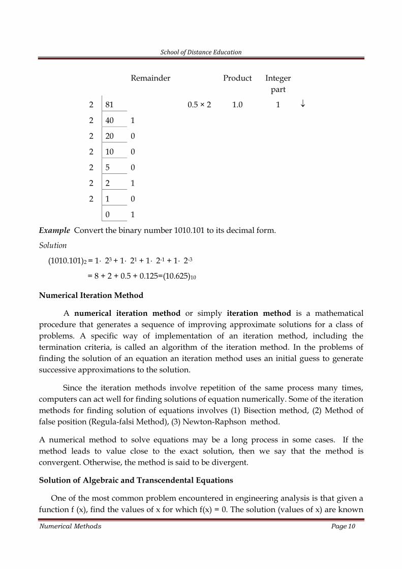
Example Convert the decimal number (which is in the base 10) 81.5 to its binary form (ofbase 2).
Solution Note that (81.5)10=8 101+1 100+5 10-1
Now 81.5 = 64+16+1+0.5=26 +24 +20 + 2-1=(1010001.1)2.
School of Distance Education
Numerical Methods Page 10
Remainder Product Integerpart
2 81
0.5 × 2 1.0 1
2 40 1
2 20 0
2 10 0
2 5 0
2 2 1
2 1 0
0 1
Example Convert the binary number 1010.101 to its decimal form.
Solution
(1010.101)2 = 1 23 + 1 21 + 1 2-1 + 1 2-3
= 8 + 2 + 0.5 + 0.125=(10.625)10
Numerical Iteration Method
A numerical iteration method or simply iteration method is a mathematicalprocedure that generates a sequence of improving approximate solutions for a class ofproblems. A specific way of implementation of an iteration method, including thetermination criteria, is called an algorithm of the iteration method. In the problems offinding the solution of an equation an iteration method uses an initial guess to generatesuccessive approximations to the solution.
Since the iteration methods involve repetition of the same process many times,computers can act well for finding solutions of equation numerically. Some of the iterationmethods for finding solution of equations involves (1) Bisection method, (2) Method offalse position (Regula-falsi Method), (3) Newton-Raphson method.
A numerical method to solve equations may be a long process in some cases. If themethod leads to value close to the exact solution, then we say that the method isconvergent. Otherwise, the method is said to be divergent.
Solution of Algebraic and Transcendental Equations
One of the most common problem encountered in engineering analysis is that given afunction f (x), find the values of x for which f(x) = 0. The solution (values of x) are known
School of Distance Education
Numerical Methods Page 11
as the roots of the equation f(x) = 0, or the zeroes of the function f (x). The roots ofequations may be real or complex.
In general, an equation may have any number of (real) roots, or no roots at all. Forexample, sin x – x = 0 has a single root, namely, x = 0, whereas tan x – x = 0 has infinitenumber of roots (x = 0, ± 4.493, ± 7.725, …).
Algebraic and Transcendental Equations
f(x) = 0 is called an algebraic equation if the corresponding ( )f x is a polynomial. Anexample is 7x2 + x - 8 = 0. ( ) 0f x is called transcendental equation if the ( )f x containstrigonometric, or exponential or logarithmic functions. Examples of transcendentalequations are sin x – x = 0, tan 0 x x and 37 log(3 6) 3 cos tan 0.xx x e x x
There are two types of methods available to find the roots of algebraic andtranscendental equations of the form f (x) = 0.
1. Direct Methods: Direct methods give the exact value of the roots in a finite number ofsteps. We assume here that there are no round off errors. Direct methods determine all theroots at the same time.
2. Indirect or Iterative Methods: Indirect or iterative methods are based on the concept ofsuccessive approximations. The general procedure is to start with one or more initialapproximation to the root and obtain a sequence of iterates kx which in the limitconverges to the actual or true solution to the root. Indirect or iterative methodsdetermine one or two roots at a time. The indirect or iterative methods are furtherdivided into two categories: bracketing and open methods. The bracketing methodsrequire the limits between which the root lies, whereas the open methods require theinitial estimation of the solution. Bisection and False position methods are two knownexamples of the bracketing methods. Among the open methods, the Newton-Raphson ismost commonly used. The most popular method for solving a non-linear equation is the
Newton-Raphson method and this method has a high rate of convergence to a solution.
In this chapter and in the coming chapters, we present the following indirect or iterativemethods with illustrative examples:
1. Fixed Point Iteration Method
2. Bisection Method
3. Method of False Position (Regula Falsi Method)
4. Newton-Raphson Method (Newton’s method)
School of Distance Education
Numerical Methods Page 12
Fixed Point Iteration Method
Consider
( ) 0f x … (1)
Transform (1) to the form,
( ).x x …(2)
Take an arbitrary x0 and then compute a sequence x1, x2, x3, . . . recursively from arelation of the form
1 ( )n nx x ( 0, 1, )n … (3)
A solution of (2) is called fixed point of . To a given equation (1) there maycorrespond several equations (2) and the behaviour, especially, as regards speed ofconvergence of iterative sequences x0, x1, x2, x3, . . . may differ accordingly.
Example Solve 2( ) 3 1 0,f x x x by fixed point iteration method.
Solution
Write the given equation as
2 3 1x x or 3 1/x x .
Choose 1( ) 3xx
. Then2
1( ) andx
x ( ) 1 x on the interval (1, 2).
Hence the iteration method can be applied to the Eq. (3).
The iterative formula is given by
113n
n
xx (n = 0, 1, 2, . . . )
Starting with, 0 1x , we obtain the sequence
x0=1.000, x1 =2.000, x2 =2.500, x3 = 2.600, x4 =2.615, . . .
Question : Under what assumptions on and 0 ,x does Algorithm 1 converge ? Whendoes the sequence ( )nx obtained from the iterative process (3) converge ?
We answer this in the following theorem, that is a sufficient condition forconvergence of iteration process
School of Distance Education
Numerical Methods Page 13
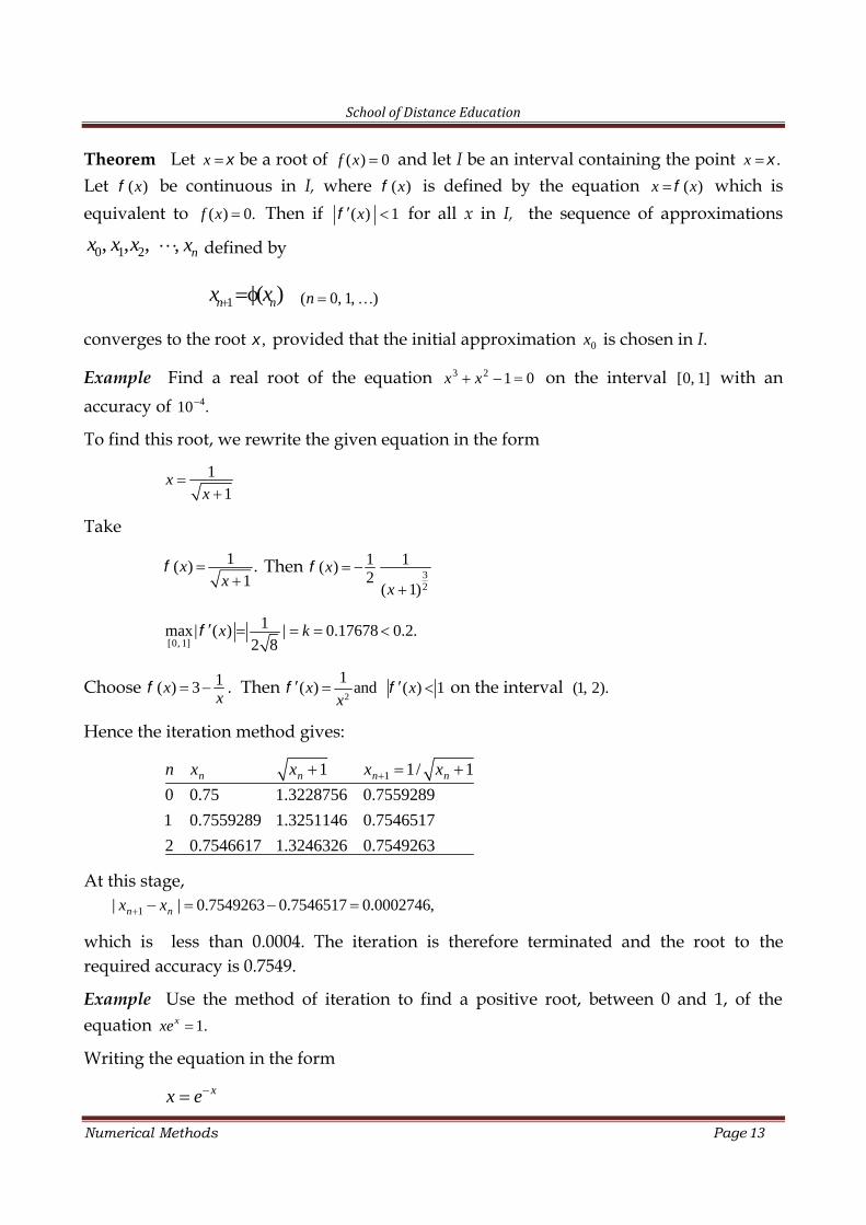
Theorem Let x be a root of ( ) 0f x and let I be an interval containing the point .x
Let ( )x be continuous in I, where ( )x is defined by the equation ( )x x which isequivalent to ( ) 0.f x Then if ( ) 1 x for all x in I, the sequence of approximations
0 1 2, , ,x x x , nx defined by
1 ( )n nx x ( 0, 1, )n
converges to the root , provided that the initial approximation 0x is chosen in I.
Example Find a real root of the equation 3 2 1 0 x x on the interval [0, 1] with anaccuracy of 410 .
To find this root, we rewrite the given equation in the form
11
xx
Take
1( ) .1
xx
Then32
1 1( )2
( 1)
x
x
[0, 1]
1max| ( ) | 0.17678 0.2.2 8
x k
Choose 1( ) 3xx
. Then2
1( ) andx
x ( ) 1x on the interval (1, 2).
Hence the iteration method gives:
11 1/ 1
0 0.75 1.3228756 0.7559289
1 0.7559289 1.3251146 0.7546517
2 0.7546617 1.3246326 0.7549263
n n n nn x x x x
At this stage,1| | 0.7549263 0.7546517 0.0002746, n nx x
which is less than 0.0004. The iteration is therefore terminated and the root to therequired accuracy is 0.7549.
Example Use the method of iteration to find a positive root, between 0 and 1, of theequation 1.xxe
Writing the equation in the form
xx e
School of Distance Education
Numerical Methods Page 14
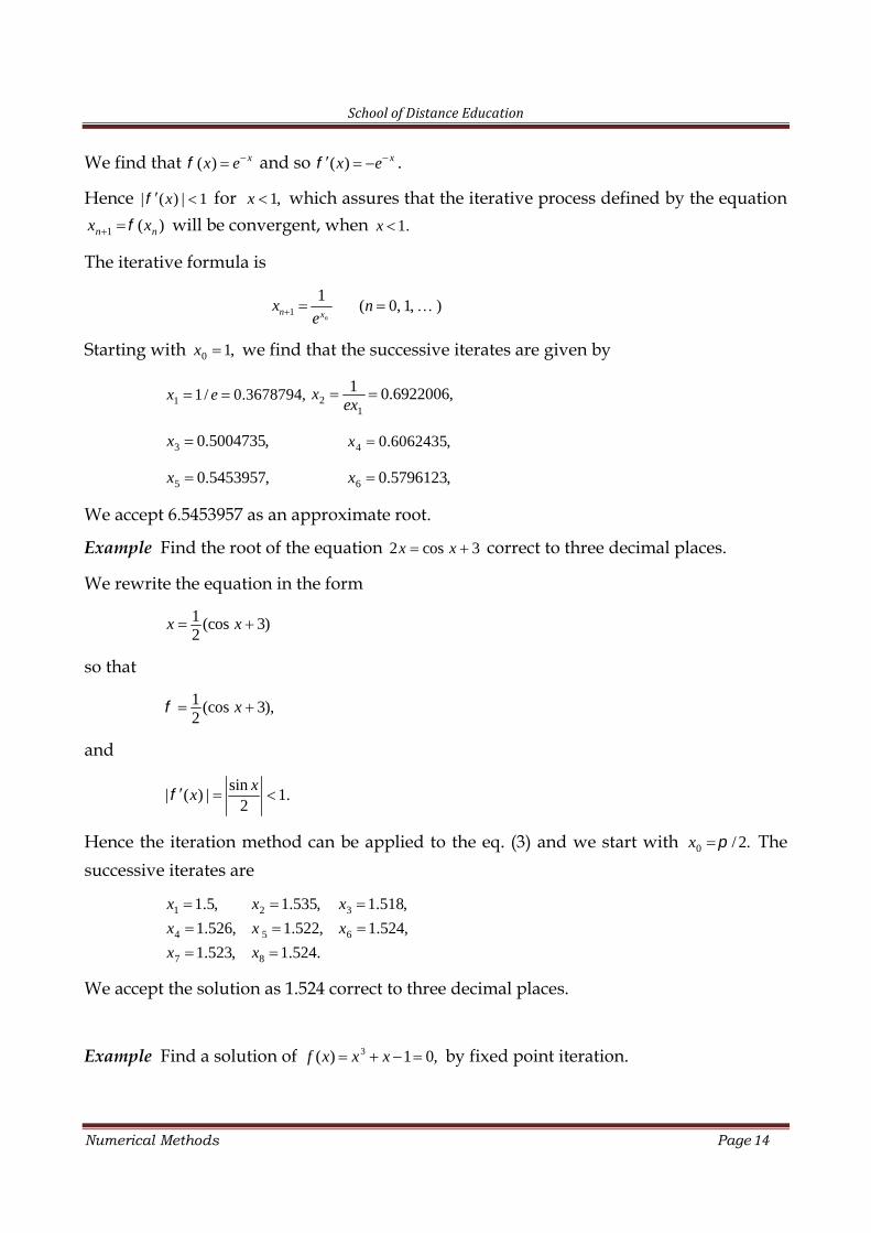
We find that ( ) xx e and so ( ) xx e .
Hence | ( ) | 1 x for 1,x which assures that the iterative process defined by the equation
1 ( ) n nx x will be convergent, when 1.x
The iterative formula is
1
1n
n xx
e ( 0, 1, )n
Starting with 0 1,x we find that the successive iterates are given by
1 1/ 0.3678794, x e 21
1 0.6922006,xex
3 0.5004735,x 4 0.6062435,x
5 0.5453957,x 6 0.5796123,x
We accept 6.5453957 as an approximate root.
Example Find the root of the equation 2 cos 3 x x correct to three decimal places.
We rewrite the equation in the form
1 (cos 3)2 x x
so that
1 (cos 3),2
x
and
sin| ( ) | 1.
2 x
x
Hence the iteration method can be applied to the eq. (3) and we start with 0 / 2.x Thesuccessive iterates are
1 2 3
4 5 6
7 8
1.5, 1.535, 1.518,
1.526, 1.522, 1.524,
1.523, 1.524.
x x x
x x x
x x
We accept the solution as 1.524 correct to three decimal places.
Example Find a solution of 3( ) 1 0,f x x x by fixed point iteration.
School of Distance Education
Numerical Methods Page 15
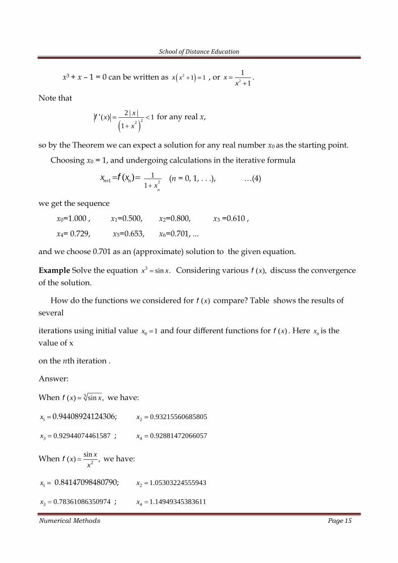
x3 + x – 1 = 0 can be written as 2 1 1xx , or2
1
1x
x
.
Note that
22
2 | |( ) 1
1
xx
x
for any real x,
so by the Theorem we can expect a solution for any real number x0 as the starting point.
Choosing x0 = 1, and undergoing calculations in the iterative formula
1 ( )n nx x 2
1
1n
x(n = 0, 1, . . .), …(4)
we get the sequence
x0=1.000 , x1=0.500, x2=0.800, x3 =0.610 ,
x4= 0.729, x5=0.653, x6=0.701, ...
and we choose 0.701 as an (approximate) solution to the given equation.
Example Solve the equation 3 sin .x x Considering various ( ),x discuss the convergenceof the solution.
How do the functions we considered for ( )x compare? Table shows the results ofseveral
iterations using initial value 0 1x and four different functions for ( )x . Here nx is thevalue of x
on the nth iteration .
Answer:
When 3( ) sin ,x x we have:
1x 0.94408924124306; 2 0.93215560685805x
3 0.92944074461587x ; 4 0.92881472066057x
When2
sin( ) ,
xx
x we have:
1x 0.84147098480790; 2 1.05303224555943x
3 0.78361086350974x ; 4 1.14949345383611x
School of Distance Education
Numerical Methods Page 16
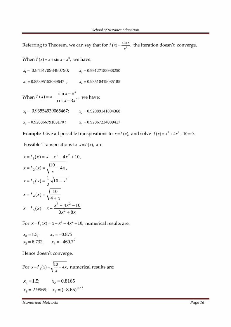
Referring to Theorem, we can say that for2
sin( ) ,
xx
x the iteration doesn’t converge.
When 3( ) sin ,x x x x we have:
1x 0.84147098480790; 2 0.99127188988250x
3 0.85395152069647x ; 4 0.98510419085185x
When3
2
sin( ) ,
cos 3
x xx x
x x
we have:
1x 0.93554939065467; 2 0.92989141894368x
3 0.92886679103170x ; 4 0.92867234089417x
Example Give all possible transpositions to ( ),x x and solve 3 2( ) 4 10 0.f x x x
Possible Transpositions to ( ),x x are
3 21
2
33
4
3 2
5 2
( ) 4 10,
10( ) 4 ,
1( ) 10
2
10( )
4
4 10( )
3 8
x x x x x
x x xx
x x x
x xx
x xx x x
x x
For 3 21( ) 4 10,x x x x x numerical results are:
0 2
3 4
1.5; 0.875
6.732; 469.7
x x
x x
;
Hence doesn’t converge.
For 210
( ) 4 ,x x xx
numerical results are:
0 2
1/ 23 4
1.5; 0.8165
2.9969; ( 8.65)
x x
x x
;
School of Distance Education
Numerical Methods Page 17
For 33
1( ) 10 ,
2x x x numerical results are:
0 2
3 4
1.5; 1.2869
1.4025; 1.3454
x x
x x
;
Exercises
Solve the following equations by iteration method:
1sin
1
xx
x
x4 = x + 0.15
3 cos 2 0x x ,0353 xx
3 1 0x x 31 36
x x
103 6 logx x 31 35
x x
102 log 7x x 3 22 10 20x x x
2sin x x cos 3 1x x
3 2 100x x 3 sin xx x e
School of Distance Education
Numerical Methods Page 18
2
BISECTION AND REGULA FALSI METHODS
Bisection Method
The bisection method is one of the bracketing methods for finding roots of an equation.For a given a function f(x), guess an interval which might contain a root and perform anumber of iterations, where, in each iteration the interval containing the root is get halved.
The bisection method is based on the intermediate value theorem for continuousfunctions.
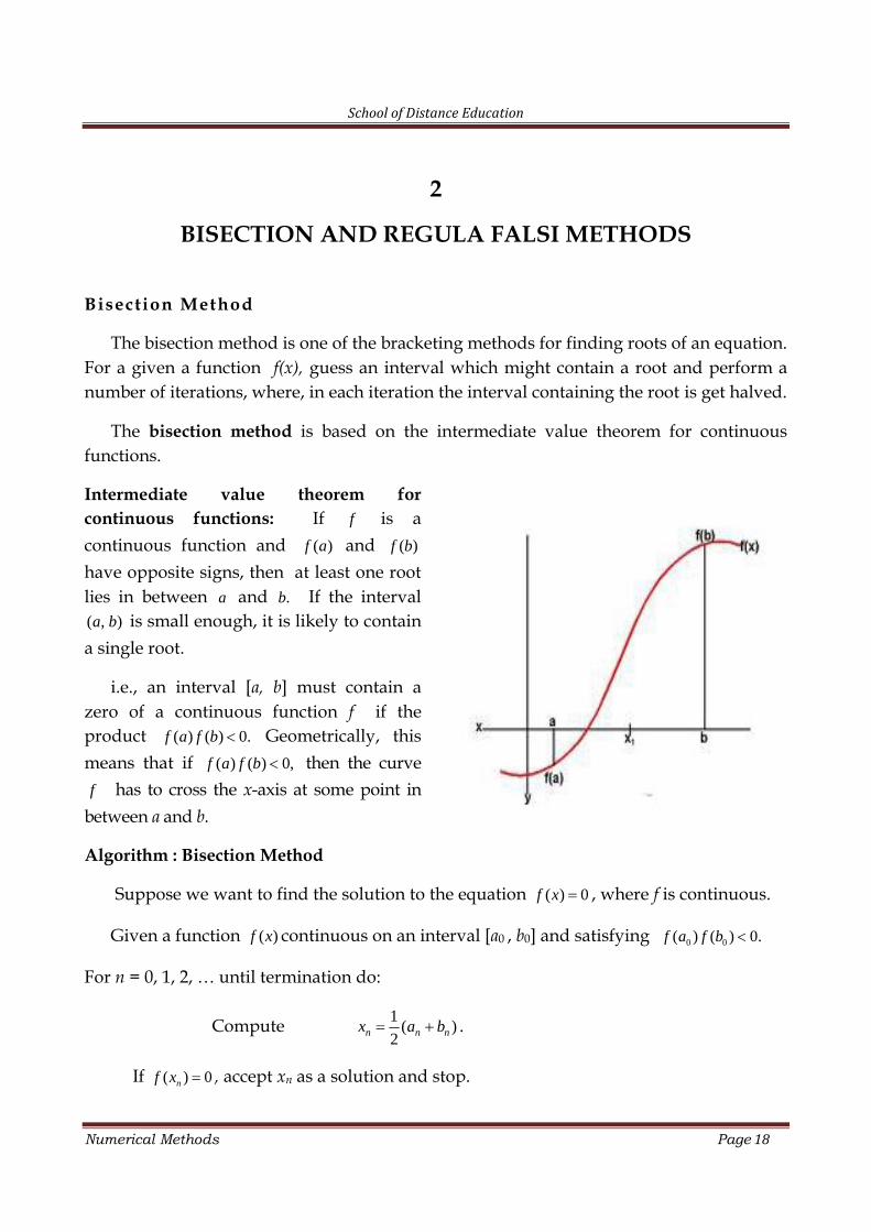
Intermediate value theorem forcontinuous functions: If f is acontinuous function and ( )f a and ( )f b
have opposite signs, then at least one rootlies in between a and .b If the interval( , )a b is small enough, it is likely to containa single root.
i.e., an interval [a, b] must contain azero of a continuous function f if theproduct ( ) ( ) 0.f a f b Geometrically, thismeans that if ( ) ( ) 0,f a f b then the curvef has to cross the x-axis at some point in
between a and b.
Algorithm : Bisection Method
Suppose we want to find the solution to the equation ( ) 0f x , where f is continuous.
Given a function ( )f x continuous on an interval [a0 , b0] and satisfying 0 0( ) ( ) 0.f a f b
For n = 0, 1, 2, … until termination do:
Compute 1( )
2 n n nx a b .
If ( ) 0nf x , accept xn as a solution and stop.
School of Distance Education
Numerical Methods Page 19
Else continue.
If ( ) ( ) 0n nf a f x , a root lies in the interval ( , )n na x .
Set 1 1, n n n na a b x .
If ( ) ( ) 0,n nf a f x a root lies in the interval ( , )n nx b .
Set 1 1, n n n na x b b .
Then ( ) 0f x for some x in 1 1[ , ]n na b .
Test for termination.
Criterion for termination
A convenient criterion is to compute the percentage error r defined by
100%.
r r
rr
x xx
where rx is the new value of rx . The computations can be terminated when r becomesless than a prescribed tolerance, say .p In addition, the maximum number of iterations
may also be specified in advance.
Some other termination criteria are as follows:
Termination after N steps (N given, fixed)
Termination if xn+1 xn ( > 0 given)
Termination if f(xn) ( >0 given).
In this chapter our criterion for termination is terminate the iteration process aftersome finite steps. However, we note that this is generally not advisable, as the steps maynot be sufficient to get an approximate solution.
Example Solve x3 – 9x+1 = 0 for the root between x = 2 and x = 4, by bisection method.
Given 3( ) 9 1f x x x . Now (2) 9, (4) 29f f so that (2) (4) 0f f and hence a root liesbetween 2 and 4.
Set a0 = 2 and b0 = 4. Then
School of Distance Education
Numerical Methods Page 20
0 0
0
( ) 2 4 32 2
a bx
and 0( ) (3) 1f x f .
Since (2) (3) 0f f , a root lies between 2 and 3, hence we set a1 = a0 = 2 and 1 0 3b x . Then
1 11
( ) 2 32.5
2 2
a bx
and 1( ) (2.5) 5.875f x f
Since (2) (2.5) 0,f f a root lies between 2.5 and 3, hence we set 2 1 2.5a x and 2 1 3b b .
Then 2 2
2
( ) 2.5 3 2.752 2
a bx
and 2( ) (2.75) 2.9531.f x f
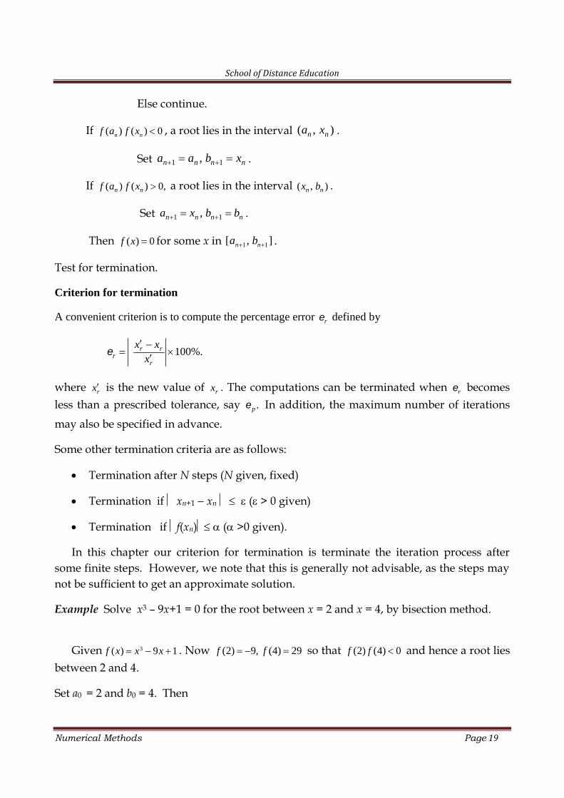
The steps are illustrated in the following table.
n nx ( )nf x
0 3 1.0000
1 2.5 5.875
2 2.75 2.9531
3 2.875 1.1113
4 2.9375 0.0901
Example Find a real root of the equation 3( ) 1 0. f x x x
Since (1)f is negative and (2)f positive, a root lies between 1 and 2 and therefore we take 0 3/ 2 1.5.x Then
027 3 15( )8 2 8
f x is positive and hence (1) (1.5) 0f f and Hence the root lies between 1
and 1.5 and we obtain
11 1.5 1.25
2 x
1( ) 19 / 64, f x which is negative and hence (1) (1.25) 0f f and hence a root lies between1.25 and 1.5. Also,
School of Distance Education
Numerical Methods Page 21
21.25 1.5 1.375
2 x
The procedure is repeated and the successive approximations are
3 1.3125,x 4 1.34375,x 5 1.328125,x etc.
Example Find a positive root of the equation 1,xxe which lies between 0 and 1.
Let ( ) 1. xf x xe Since (0) 1 f and (1) 1.718,f it follows that a root lies between 0 and 1.Thus,
00 1 0.5
2x .
Since (0.5)f is negative, it follows that a root lies between 0.5 and 1. Hence the new root is0.75, i.e.,
1.5 1 0.75.
2x
Since 1( )f x is positive, a root lies between 0.5 and 0.75 . Hence
2
.5 .750.625
2x
Since 2( )f x is positive, a root lies between 0.5 and 0.625. Hence
3
.5 .6250.5625.
2x
We accept 0.5625 as an approximate root.
Merits of bisection method
a) The iteration using bisection method always produces a root, since the methodbrackets the root between two values.
b) As iterations are conducted, the length of the interval gets halved. So one canguarantee the convergence in case of the solution of the equation.
c) the Bisection Method is simple to program in a computer.

School of Distance Education
Numerical Methods Page 22
Demerits of bisection method
a) The convergence of the bisection method is slow as it is simply based onhalving the interval.
b) Bisection method cannot be applied over an interval where there is adiscontinuity.
c) Bisection method cannot be applied over an interval where the function takesalways values of the same sign.
d) The method fails to determine complex roots.
e) If one of the initial guesses 0a or 0b is closer to the exact solution, it will takelarger number of iterations to reach the root.
Exercises
Find a real root of the following equations by bisection method.
1. 3 1 sinx x 2. 3 21.2 4 48x x x
3. 3xe x 4. 3 4 9 0x x
5. 3 3 1 0x x 6. 3 cos 1x x
7. 3 2 1 0x x 8. 2 3 cosx x
9. 4 3x 10. x3 5x = 6
11. cos x x 12. ,0323 xxx
13. x4 = x + 0.15 near x = 0.
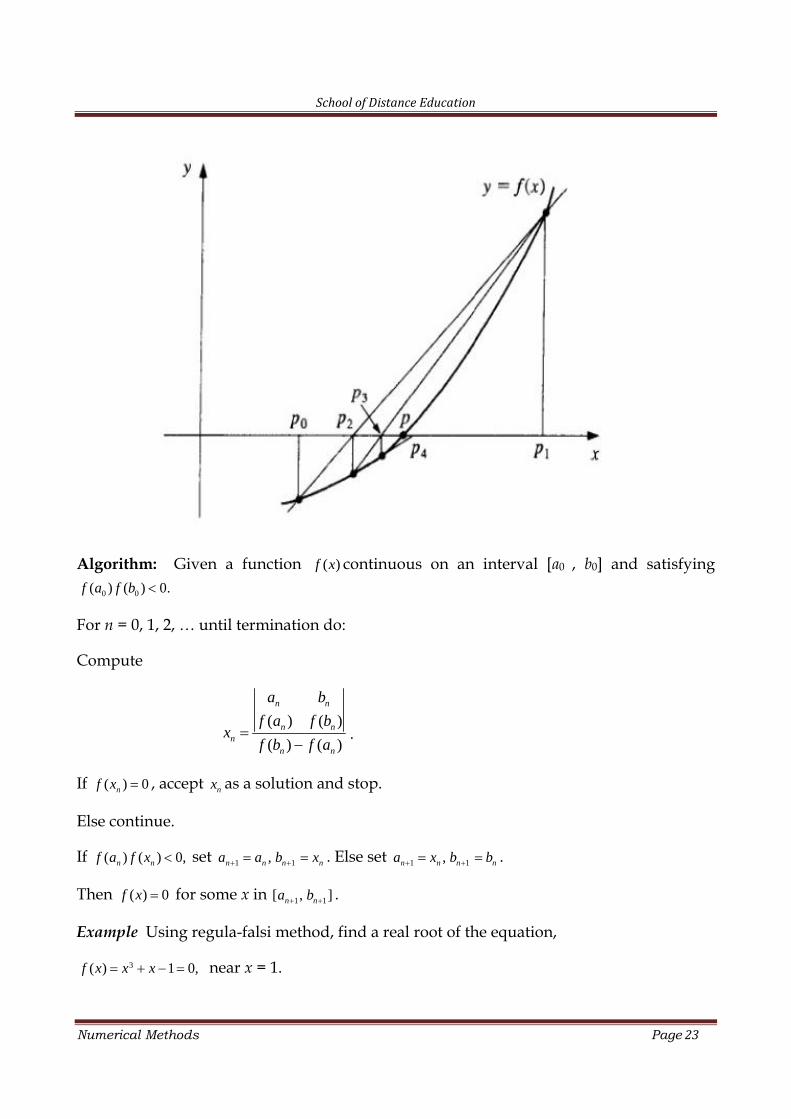
Regula Falsi method or Method of False Position
This method is also based on the intermediate value theorem. In this method also, asin bisection method, we choose two points an and bn such that ( )nf a and ( )nf b are ofopposite signs (i.e., ( ) ( ) 0)n nf a f b . Then, intermediate value theorem suggests that a zeroof f lies in between an and bn, if f is a continuous function.
School of Distance Education
Numerical Methods Page 23
Algorithm: Given a function ( )f x continuous on an interval [a0 , b0] and satisfying
0 0( ) ( ) 0.f a f b
For n = 0, 1, 2, … until termination do:
Compute
( ) ( )
( ) ( )
n n
n nn
n n
a b
f a f bx
f b f a
.
If ( ) 0nf x , accept nx as a solution and stop.
Else continue.
If ( ) ( ) 0,n nf a f x set 1 1,n n n na a b x . Else set 1 1,n n n na x b b .
Then ( ) 0f x for some x in 1 1[ , ]n na b .
Example Using regula-falsi method, find a real root of the equation,
3( ) 1 0,f x x x near x = 1.
School of Distance Education
Numerical Methods Page 24
Here note that f(0) = -1 and (0) 1f . Hence (0) (1) 0f f , so by intermediate valuetheorem a root lies in between 0 and 1. We search for that root by regula falsi method andwe will get an approximate root.
Set a0 = 0 and b0 = 1. Then
0 0
0 0
0
0 0
0 11 1
0.51 1
a b
f a f bx
f b f a
and 0( ) (0.5) 0.375f x f .
Since (0) (0.5) 0f f , a root lies between 0.5 and 1. Set 1 0 0.5a x and 1 0 1b b .
Then
1 1
1 1
1
1 1
0.5 10.375 1
0.63641 0.375
a b
f a f bx
f b f a
and 1( ) (0.6364) 0.1058.f x f
Since 1(0.6364) ( ) 0f f x , a root lies between 1x and 1 and hence we set 2 1 0.6364a x and
2 1 1.b b Then
2 2
2 2
2
2 2
0.6364 10.1058 1
0.67121 0.1058
a b
f a f bx
f b f a
and 2( ) (0.6712) 0.0264f x f
Since (0.6712) (0.6364) 0,f f a root lies between 2x and 1, and hence we set 3 2 0.6364a x
and 3 1 1b b .
Then
3 3
3 3
3
3 3
0.6712 10.0264 1
0.67961 0.0264
a b
f a f bx
f b f a
and 3( ) (0.6796) 0.0063 0f x f .
School of Distance Education
Numerical Methods Page 25
Since (0.6796) 0.0000f we accept 0.6796 as an (approximate) solution of 013 xx .
Example Given that the equation 2.2 69x has a root between 5 and 8. Use the method ofregula-falsi to determine it.
Let 2.2( ) 69.f x x We find
(5) 3450675846 f and (8) 28.00586026. f
1
5 8
(5) (8) 5(28.00586026) 8( 34.50675846)(8) (5) 28.00586026 34.50675846)
f fx
f f 6.655990062 .
Now, 1( ) 4.275625415 f x and therefore, 1(5) ( ) 0f f x and hence the root lies between6.655990062 and 8.0. Proceeding similarly,
2 6.83400179,x 3 6.850669653,x
The correct root is 3 6.8523651 , x so that 3x is correct to these significant figures. Weaccept 6.850669653 as an approximate root.
Theoretical Exercises with Answers:
1. What is the difference between algebraic and transcendental equations?
Ans: An equation ( ) 0f x is called an algebraic equation if the corresponding ( )f x
is a polynomial, while, ( ) 0f x is called transcendental equation if the ( )f x
contains trigonometric, or exponential or logarithmic functions.
2. Why we are using numerical iterative methods for solving equations?
Ans: As analytic solutions are often either too tiresome or simply do not exist, weneed to find an approximate method of solution. This is where numerical analysiscomes into the picture.
3. Based on which principle, the bisection and regula-falsi method is developed?
Ans: These methods are based on the intermediate value theorem for continuousfunctions: stated as , “If f is a continuous function and ( )f a and ( )f b haveopposite signs, then at least one root lies in between a and .b If the interval ( , )a b
is small enough, it is likely to contain a single root. ”
4. What are the advantages and disadvantages of the bracketing methods like bisectionand regula-falsi?
School of Distance Education
Numerical Methods Page 26
Ans: (i) The bisection and regula-falsi method is always convergent. Since themethod brackets the root, the method is guaranteed to converge. The maindisadvantage is, if it is not possible to bracket the roots, the methods cannotapplicable. For example, if ( )f x is such that it always takes the values with samesign, say, always positive or always negative, then we cannot work with bisectionmethod. Some examples of such functions are
2( )f x x which take only non-negative values and
2( )f x x , which take only non-positive values.
Exercises
Find a real root of the following equations by false position method:
1. 3 5 6x x 2. 4 xx e
3. 10log 1.2x x 4. tan tanh 0x x
5. sinxe x 6. 3 5 7 0x x
7. 3 22 10 20 0x x x 8. 102 log 7x x
9. cosxxe x 10. 3 5 1 0x x
11. 3xe x 12. 2 log 12ex x
13. 3 cos 1x x 14. 2 3sin 5x x
15. 2 cos 3x x 16. 3xxe
17. cos x x 18. 3 5 3 0x x
Ramanujan’s Method
We need the following Theorem:
Binomial Theorem: If n is any rational number and 1x , then
2 ( 1) . . . ( ( 1))( 1)1 1 . . . . . .
1 1 2 1 2 . . .n rn n n rn nnx x x x
r
School of Distance Education
Numerical Methods Page 27
In particular,
1 2 31 1 . . . 1 . . .n nx x x x x
and 1 2 31 1 . . . . . .nx x x x x
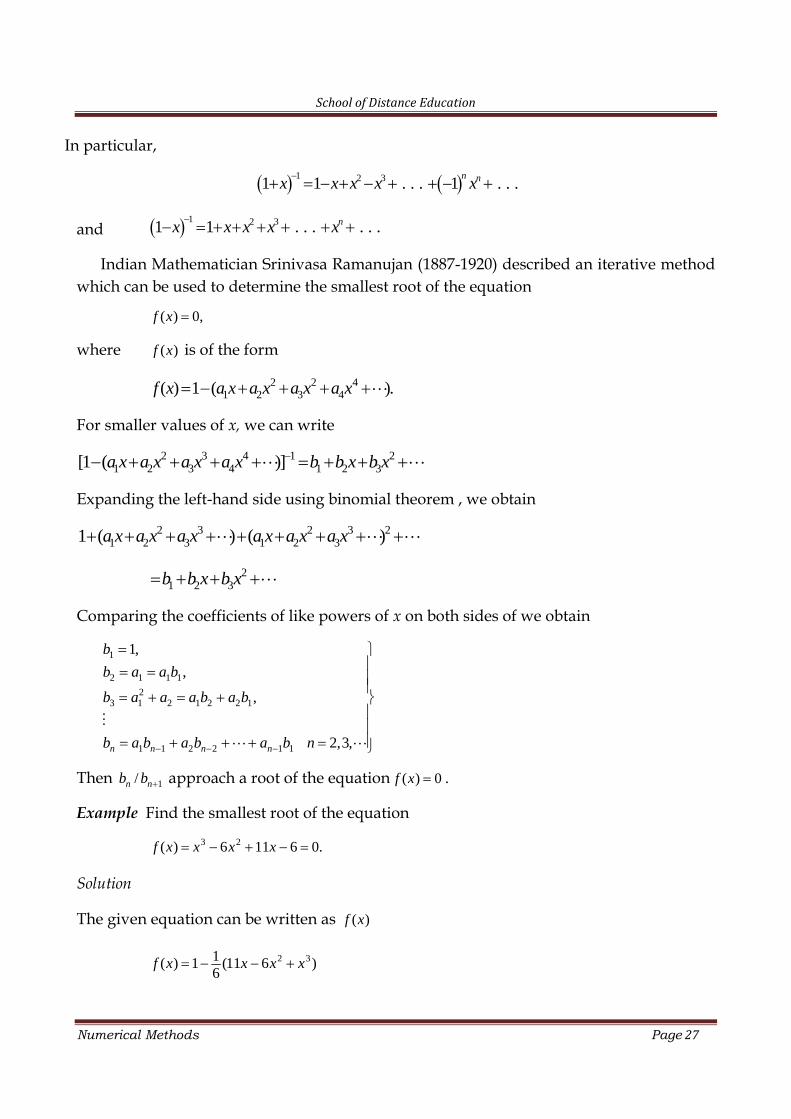
Indian Mathematician Srinivasa Ramanujan (1887-1920) described an iterative methodwhich can be used to determine the smallest root of the equation
( ) 0,f x
where ( )f x is of the form
2 2 41 2 3 4( ) 1 ( ).f x a x a x a x a x
For smaller values of x, we can write
2 3 4 1 21 2 3 4 1 2 3[1 ( )]a x a x a x a x b b x b x
Expanding the left-hand side using binomial theorem , we obtain
2 3 2 3 21 2 3 1 2 31 ( ) ( )a x a x a x a x a x a x
21 2 3b b x b x
Comparing the coefficients of like powers of x on both sides of we obtain
1
2 1 1 1
23 1 2 1 2 2 1
1 1 2 2 1 1
1,
,
,
2,3,n n n n
b
b a a b
b a a a b a b
b a b a b a b n
Then 1/n nb b approach a root of the equation ( ) 0f x .
Example Find the smallest root of the equation
3 2( ) 6 11 6 0.f x x x x
Solution
The given equation can be written as ( )f x
2 31( ) 1 (11 6 )6
f x x x x
School of Distance Education
Numerical Methods Page 28
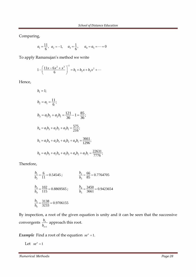
Comparing,
111,6
a 2 1,a 31 ,6
a 4 5 0a a
To apply Ramanujan’s method we write
12 32
1 2 311 61
6x x x b b x b x
Hence,
1 1;b
2 111;6
b a
3 1 2 2 1121 851 ;36 36
b a b a b
4 1 3 2 2 3 1575;216
b a b a b a b
5 1 4 2 3 3 2 4 13661;1296
b a b a b a b a b
6 1 5 2 4 3 3 4 2 5 122631;7776
b a b a b a b a b a b
Therefore,
1
2
6 0.5454511
bb ; 2
3
66 0.776470585
bb
3
4
102 0.8869565115
bb ; 4
5
3450 0.94236543661
bb
5
6
3138 0.97061553233
bb
By inspection, a root of the given equation is unity and it can be seen that the successive
convergents1
n
n
b
b approach this root.
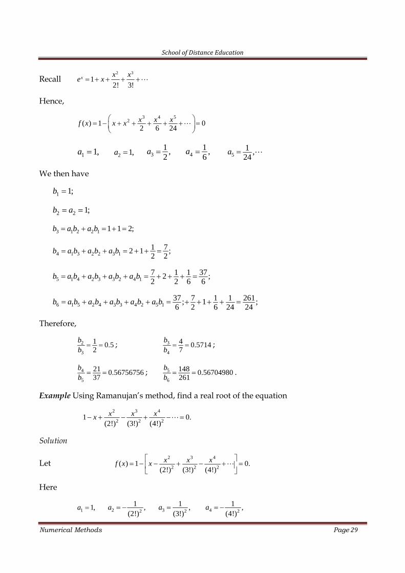
Example Find a root of the equation 1.xxe
Let 1xxe
School of Distance Education
Numerical Methods Page 29
Recall2 3
12! 3!
x x xe x
Hence,
3 4 52( ) 1 0
2 6 24x x xf x x x
1 1,a 2 1,a 31 ,2
a 41 ,6
a 51 ,24
a
We then have
1 1;b
2 2 1;b a
3 1 2 2 1 1 1 2;b a b a b
4 1 3 2 2 3 11 72 1 ;2 2
b a b a b a b
5 1 4 2 3 3 2 4 17 1 1 372 ;2 2 6 6
b a b a b a b a b
6 1 5 2 4 3 3 4 2 5 137 7 1 1 261; 1 ;6 2 6 24 24
b a b a b a b a b a b
Therefore,
2
3
1 0.52
bb ; 3
4
4 0.57147
bb ;
4
5
21 0.5675675637
bb ; 5
6
148 0.56704980261
bb .
Example Using Ramanujan’s method, find a real root of the equation
2 3 4
2 2 21 0.
(2!) (3!) (4!)x x xx
Solution
Let2 3 4
2 2 2( ) 1 0.
(2!) (3!) (4!)x x xf x x
Here
1 1,a 2 21 ,
(2!)a 3 2
1 ,(3!)
a 4 21 ,
(4!)a
School of Distance Education
Numerical Methods Page 30
5 21 ,
(5!)a 6 2
1 ,(6!)
a
Writing
12 3 4
21 2 32 2
1(2!) (3!) (4!)x x xx b b x b x
,
we obtain
1 1,b
2 1 1,b a
3 1 2 2 1 21 31 ;
4(2!)b a b a b
4 1 3 2 2 3 1 2 23 1 1 3 1 14 4 4 36(2!) (3!)
b a b a b a b 19 ,36
5 1 4 2 3 3 2 4 1b a b a b a b a b
19 1 3 1 1 2111 .36 4 4 36 576 576
It follows
1
2
1;bb 2
3
4 1.333 ;3
bb
3
4
3 36 27 1.4210 ,4 19 19
bb 4
5
19 576 1.4408 ,36 211
bb
where the last result is correct to three significant figures.
Example Find a root of the equation sin 1 .x x
Using the expansion of sin ,x the given equation may be written as
3 5 7
( ) 1 0.3! 5! 7!x x xf x x x
Here
School of Distance Education
Numerical Methods Page 31
1 2,a 2 0,a 31 ,6
a 4 0,a
51 ,
120a 6 0,a 7
1 ,5040
a
we write
13 5 7
21 2 31 2
6 120 5040x x xx b b x b x
We then obtain
1 1;b
2 1 2;b a
3 1 2 2 1 4;b a b a b
4 1 3 2 2 3 11 478 ;6 6
b a b a b a b
5 1 4 2 3 3 2 4 146 ;3
b a b a b a b a b
6 1 5 2 4 3 3 4 2 5 13601;120
b a b a b a b a b a b
Therefore,
1
2
1 ;2
bb 2
3
1 ;2
bb
3
4
24 0.510638227
bb 4
5
47 0.510869592
bb
5
6
1840 0.51096913601
bb .
The root, correct to four decimal places is 0.5110
Exercises
1. Using Ramanujan’s method, obtain the first-eight convergents of the equation2 3 4
2 2 21 0
(2!) (3!) (4!)
x x xx
2. Using Ramanujan’s method, find the real root of the equation 3 1.x x
School of Distance Education
Numerical Methods Page 32
3
NEWTON RAPHSON ETC..
The Newton-Raphson method, or Newton Method, is a powerful technique for solvingequations numerically. Like so much of the differential calculus, it is based on the simpleidea of linear approximation.
Newton – Raphson Method
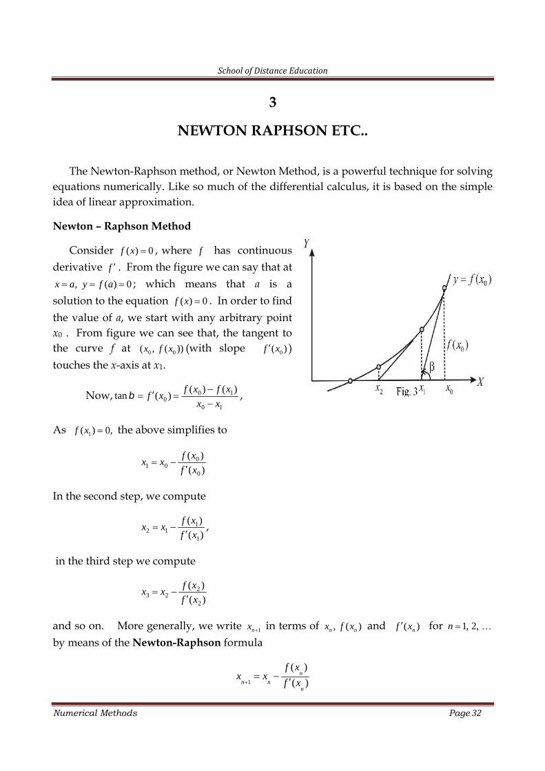
Consider ( ) 0f x , where f has continuousderivative f . From the figure we can say that at
, ( ) 0x a y f a ; which means that a is asolution to the equation ( ) 0f x . In order to findthe value of a, we start with any arbitrary pointx0 . From figure we can see that, the tangent tothe curve f at 0 0( , ( ))x f x (with slope 0( )f x )touches the x-axis at x1.
Now,10
100
)()()(tan
xx
xfxfxf
,
As 1( ) 0,f x the above simplifies to
)(
)(
0
001 xf
xfxx
In the second step, we compute
)(
)(
1
112 xf
xfxx
,
in the third step we compute
)(
)(
2
223 xf
xfxx
and so on. More generally, we write 1nx in terms of , ( )n nx f x and ( )nf x for 1, 2,n
by means of the Newton-Raphson formula
1
( )
( )
n
n nn
f xx x
f x
School of Distance Education
Numerical Methods Page 32
3
NEWTON RAPHSON ETC..
The Newton-Raphson method, or Newton Method, is a powerful technique for solvingequations numerically. Like so much of the differential calculus, it is based on the simpleidea of linear approximation.
Newton – Raphson Method
Consider ( ) 0f x , where f has continuousderivative f . From the figure we can say that at
, ( ) 0x a y f a ; which means that a is asolution to the equation ( ) 0f x . In order to findthe value of a, we start with any arbitrary pointx0 . From figure we can see that, the tangent tothe curve f at 0 0( , ( ))x f x (with slope 0( )f x )touches the x-axis at x1.
Now,10
100
)()()(tan
xx
xfxfxf
,
As 1( ) 0,f x the above simplifies to
)(
)(
0
001 xf
xfxx
In the second step, we compute
)(
)(
1
112 xf
xfxx
,
in the third step we compute
)(
)(
2
223 xf
xfxx
and so on. More generally, we write 1nx in terms of , ( )n nx f x and ( )nf x for 1, 2,n
by means of the Newton-Raphson formula
1
( )
( )
n
n nn
f xx x
f x
School of Distance Education
Numerical Methods Page 33
The refinement on the value of the rootn
x is terminated by any of the following conditions.
(i) Termination after a pre-fixed number of steps
(ii) After n iterations where, 1
0nn
x x for a given , or
(iii) After n iterations, where ( ) 0n
f x for a given .
Termination after a fixed number of steps is not advisable, because a fine approximation cannot beensured by a fixed number of steps.
Algorithm: The steps of the Newton-Raphson method to find the root of an equation 0xf are
1. Evaluate xf
2. Use an initial guess of the root, ix , to estimate the new value of the root, 1ix , as
i
iii xf
xf = xx
1
3. Find the absolute relative approximate error a as
0101
1
i
iia x
xx =
4. Compare the absolute relative approximate error with the pre-specified relative error
tolerance, s . If a > s then go to Step 2, else stop the algorithm. Also, check if the
number of iterations has exceeded the maximum number of iterations allowed. If so, oneneeds to terminate the algorithm and notify the user.
The method can be used for both algebraic and transcendental equations, and it also workswhen coefficients or roots are complex. It should be noted, however, that in the case of analgebraic equation with real coefficients, a complex root cannot be reached with a real startingvalue.
Example Set up a Newton iteration for computing the square root of a given positivenumber. Using the same find the square root of 2 exact to six decimal places.
Let c be a given positive number and let x be its positive square root, so that cx . Thencx 2 or
School of Distance Education
Numerical Methods Page 34
2( ) 0f x x c
xxf 2)(
Using the Newton’s iteration formula we have
2
1 2n
n nn
x cx x
x
or1 2 2
n
nn
x cxx
or1
1 , 0.1, 2,2n n
n
cx x nx
,
Now to find the square root of 2, let c = 2, so that
1
1 2 , 0, 1, 2,2n n
n
x x nx
Choose 0 1x . Then
x1 = 1.500000, x2 = 1.416667, x3 = 1.414216, x4 = 1.414214, …
and accept 1.414214 as the square root of 2 exact to 6D.
Historical Note: Heron of Alexandria (60 CE?) used a pre-algebra version of the above
recurrence. It is still at the heart of computer algorithms for finding square roots.
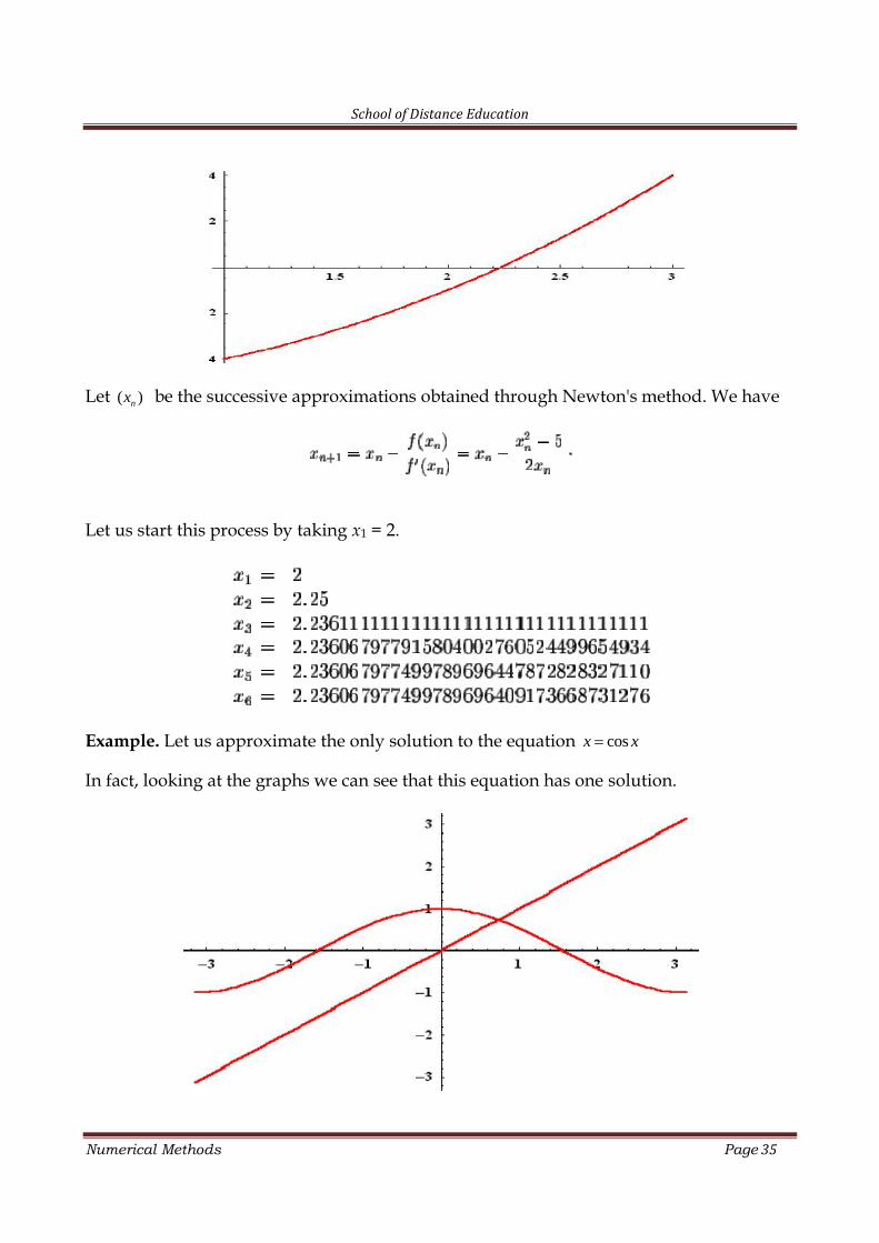
Example. Let us find an approximation to 5 to ten decimal places.
Note that 5 is an irrational number. Therefore the sequence of decimals which defines5 will not stop. Clearly 5 is the only zero of f(x) = x2 - 5 on the interval [1, 3]. See the
Picture.
School of Distance Education
Numerical Methods Page 35
Let ( )nx be the successive approximations obtained through Newton's method. We have
Let us start this process by taking x1 = 2.
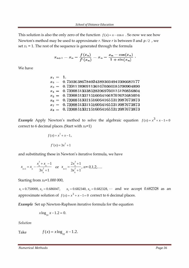
Example. Let us approximate the only solution to the equation cosx x
In fact, looking at the graphs we can see that this equation has one solution.
School of Distance Education
Numerical Methods Page 35
Let ( )nx be the successive approximations obtained through Newton's method. We have
Let us start this process by taking x1 = 2.
Example. Let us approximate the only solution to the equation cosx x
In fact, looking at the graphs we can see that this equation has one solution.
School of Distance Education
Numerical Methods Page 36
This solution is also the only zero of the function ( ) cosf x x x . So now we see howNewton's method may be used to approximate r. Since r is between 0 and / 2 , weset x1 = 1. The rest of the sequence is generated through the formula
We have
Example Apply Newton’s method to solve the algebraic equation 013)( xxxf
correct to 6 decimal places. (Start with x0=1)
3( ) 1f x x x ,
2( ) 3 1f x x
and substituting these in Newton’s iterative formula, we have
3
21
1
3 1n n
n n
n
x xx x
x
or
3
21
2 1
3 1n
n
n
xx
x
, n= 0,1,2,….
Starting from x0=1.000 000,
1 20.750000, 0.686047,x x 3 40.682340, 0.682328,x x and we accept 0.682328 as an
approximate solution of 3( ) 1 0f x x x correct to 6 decimal places.
Example Set up Newton-Raphson iterative formula for the equation
10log 1.2 0. x x
Solution
Take10
( ) log 1.2. f x x x
School of Distance Education
Numerical Methods Page 37
Noting that10 10
log log log log0.4343 ,e e
x x e x
we obtain ( ) log0.4343 1.2.e
f x x x
10( ) log log10.4343 0.4343 0.4343
ef x x x x
x
and hence the Newton’s iterative formula for the given equation is
110
log
log
( ) 0.4343 1.2
( ) 0.4343n e n
n n nn
f x x xx x x
f x x
.
Example Find the positive solution of the transcendental equation
xx sin2 .
Here xxxf sin2)( ,
so that xxf cos21)(
Substituting in Newton’s iterative formula, we have
1
2sin
1 2cosn n
n nn
x xx x
x
, 0.1, 2,n or
1
2(sin cos )
1 2cosn n n n
nn n
x x x Nx
x D
, 0.1, 2,n
where we take 2(sin cos )n n n n
N x x x and 1 2cosn n
D x , to easy our calculation. Values
calculated at each step are indicated in the following table (Starting with 0 2x ).
n xn Nn Dn xn+1
0 2.000 3.483 1.832 1.901
1 1.901 3.125 1.648 1.896
2 1.896 3.107 1.639 1.896
1.896 is an approximate solution to xx sin2 .
Example Use Newton-Raphson method to find a root of the equation 3 2 5 0. x x
Here 3( ) 2 5 f x x x and 2( ) 3 2. f x x Hence Newton’s iterative formula becomes
School of Distance Education
Numerical Methods Page 38
3`
1 2
2 5
3 2
n nn n
n
x xx x
x
Choosing 0 2,x we obtain 0( ) 1 f x and 0( ) 10. f x
112 2.1
10 x
31( ) (2.1) 2(2.1) 5 0.06,f x
and 21( ) 3(2.1) 2 11.23.f x
20.0612.1 2.094568.11.23
x
2.094568 is an approximate root.
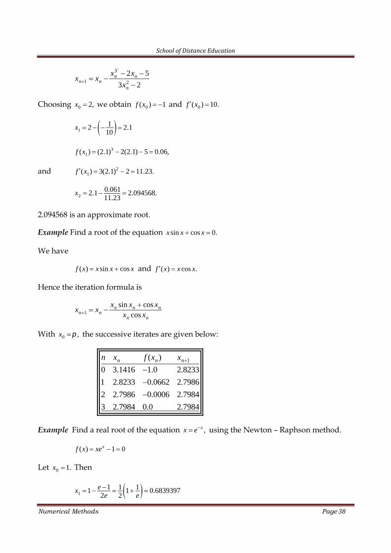
Example Find a root of the equation sin cos 0.x x x
We have
( ) sin cosf x x x x and ( ) cos .f x x x
Hence the iteration formula is
1
sin coscos
n n nn n
n n
x x xx x
x x
With 0 ,x the successive iterates are given below:
1( )
0 3.1416 1.0 2.8233
1 2.8233 0.0662 2.7986
2 2.7986 0.0006 2.7984
3 2.7984 0.0 2.7984
n n nn x f x x
Example Find a real root of the equation ,xx e using the Newton – Raphson method.
( ) 1 0xf x xe
Let 0 1.x Then
11 1 11 1 0.6839397
2 2ex
e e
School of Distance Education
Numerical Methods Page 39
Now 1( ) 0.3553424,f x and 1( ) 3.337012,f x
20.35534240.6839397 0.5774545.3.337012
x
3 0.5672297x and 4 0.5671433.x
Example f(x) = x−2+lnx has a root near x = 1.5. Use the Newton-Raphson formula toobtain a better estimate.
Here x0 = 1.5, f(1.5)= −0.5 + ln(1.5)= −0.0945
1
( 0.0945)1 5( ) 1 ; (1.5) ; 1.5 1.55673 1.6667
f x f xx
The Newton-Raphson formula can be used again: this time beginning with 1.5567 as ourinitial
2
( 0.0007)1.5567 1.5571
1.6424x
This is in fact the correct value of the root to 4 d.p.
Generalized Newton’s Method
If is a root of ( ) 0f x with multiplicity p, then the generalized Newton’s formula is
1
( ),
( )n
n nn
f xx x p
f x
Since is a root of ( ) 0f x with multiplicity p, it follows that is a root of ( ) 0f x
with multiplicity ( 1),p of ( ) 0f x with multiplicity ( 2),p and so on. Hence theexpressions
0 0 00 0 0
0 0 0
( ) ( ) ( ), ( 1) , ( 2)
( ) ( ) ( )f x f x f x
x p x p x pf x f x f x
must have the same value if there is a root with multiplicity p, provided that the initialapproximation 0x is chosen sufficiently close to the root.
Example Find a double root of the equation
3 2( ) 1 0.f x x x x
Here 2( ) 3 2 1,f x x x and ( ) 6 2.f x x With 0 0.8,x we obtain
School of Distance Education
Numerical Methods Page 40
00
0
( ) 0.0722 0.8 2 1.012,( ) (0.68)
f xx
f x
and
00
0
( ) (0.68)0.8 1.043,( ) 2.8
f xx
f x
The closeness of these values indicates that there is a doublel root near to unity. For thenext approximation, we choose 1 1.01x and obtain
11
1
( )2 1.01 0.0099 1.0001,
( )f x
xf x
and 11
1
( )1.01 0.0099 1.0001,
( )f x
xf x
Hence we conclude that there is a double root at 1.0001x which is sufficiently close to theactual root unity.
On the other hand, if we apply Newton-Raphson method with 0 0.8,x we obtain
1 0.8 0.106 0.91,x and 2 0.91 0.046 0.96.x
Exercises
1. Approximate the real root to two four decimal places of 3 5 3 0x x
2. Approximate to four decimal places 3 3
3. Find a positive root of the equation 4 2 1 0x x correct to 4 places of decimals.(Choose x0 = 1.3)
4. Explain how to determine the square root of a real number by N R method andusing it determine 3 correct to three decimal places.
5. Find the value of 2 correct to four decimals places using Newton Raphson method.
6. Use the Newton-Raphson method, with 3 as starting point, to find a fraction that iswithin 810 of 10 .
7. Design Newton iteration for the cube root. Calculate 3 7 , starting from x0 = 2 andperforming 3 steps.
8. Calculate 7 by Newton’s iteration, starting from x0 = 2 and calculating x1, x2, x3.Compare the results with the value 645751.27
School of Distance Education
Numerical Methods Page 41
9. Design a Newton’s iteration for computing kth root of a positive number c.
10. Find all real solutions of the following equations by Newton’s iteration method.
(a) sin x = .2
x (b) ln x = 1 – 2x (c) cos x x
11. Using Newton-Raphson method, find the root of the equation ,0323 xxx
correct to three decimal places
12. Apply Newton’s method to the equation
35 3 0x x
starting from the given0
2x and performing 3 steps.
13. Apply Newton’s method to the equation
4 32 34 0x x x
starting from the given0
3x and performing 3 steps.
14. Apply Newton’s method to the equation
3 23.9 4.79 1.881 0x x x
starting from the given0
1x and performing 3 steps.
Ramanujan’s Method
We need the following Theorem:
Binomial Theorem: If n is any rational number and 1x , then
2 ( 1) . . . ( ( 1))( 1)1 1 . . . . . .
1 1 2 1 2 . . .n rn n n rn nnx x x x
r
In particular,
1 2 31 1 . . . 1 . . .n nx x x x x
and 1 2 31 1 . . . . . .nx x x x x
Indian Mathematician Srinivasa Ramanujan (1887-1920) described an iterative methodwhich can be used to determine the smallest root of the equation
School of Distance Education
Numerical Methods Page 42
( ) 0,f x
where ( )f x is of the form
2 2 41 2 3 4( ) 1 ( ).f x a x a x a x a x
For smaller values of x, we can write
2 3 4 1 21 2 3 4 1 2 3[1 ( )]a x a x a x a x b b x b x
Expanding the left-hand side using binomial theorem , we obtain
2 3 2 3 21 2 3 1 2 31 ( ) ( )a x a x a x a x a x a x
21 2 3b b x b x
Comparing the coefficients of like powers of x on both sides of we obtain
1
2 1 1 1
23 1 2 1 2 2 1
1 1 2 2 1 1
1,
,
,
2,3,n n n n
b
b a a b
b a a a b a b
b a b a b a b n
Then 1/n nb b approach a root of the equation ( ) 0f x .
Example Find the smallest root of the equation
3 2( ) 6 11 6 0.f x x x x
Solution
The given equation can be written as ( )f x
2 31( ) 1 (11 6 )6
f x x x x
Comparing,
111,6
a 2 1,a 31 ,6
a 4 5 0a a
To apply Ramanujan’s method we write
12 32
1 2 311 61
6x x x b b x b x
School of Distance Education
Numerical Methods Page 43
Hence,
1 1;b
2 111;6
b a
3 1 2 2 1121 851 ;36 36
b a b a b
4 1 3 2 2 3 1575;216
b a b a b a b
5 1 4 2 3 3 2 4 13661;1296
b a b a b a b a b
6 1 5 2 4 3 3 4 2 5 122631;7776
b a b a b a b a b a b
Therefore,
1
2
6 0.5454511
bb ; 2
3
66 0.776470585
bb
3
4
102 0.8869565115
bb ; 4
5
3450 0.94236543661
bb
5
6
3138 0.97061553233
bb
By inspection, a root of the given equation is unity and it can be seen that the successive
convergents1
n
n
b
b approach this root.
Example Find a root of the equation 1.xxe
Let 1xxe
Recall2 3
12! 3!
x x xe x
Hence,
3 4 52( ) 1 0
2 6 24x x xf x x x
1 1,a 2 1,a 31 ,2
a 41 ,6
a 51 ,24
a
School of Distance Education
Numerical Methods Page 44
We then have
1 1;b
2 2 1;b a
3 1 2 2 1 1 1 2;b a b a b
4 1 3 2 2 3 11 72 1 ;2 2
b a b a b a b
5 1 4 2 3 3 2 4 17 1 1 372 ;2 2 6 6
b a b a b a b a b
6 1 5 2 4 3 3 4 2 5 137 7 1 1 261; 1 ;6 2 6 24 24
b a b a b a b a b a b
Therefore,
2
3
1 0.52
bb ; 3
4
4 0.57147
bb ;
4
5
21 0.5675675637
bb ; 5
6
148 0.56704980261
bb .
Example Using Ramanujan’s method, find a real root of the equation
2 3 4
2 2 21 0.
(2!) (3!) (4!)x x xx
Solution
Let2 3 4
2 2 2( ) 1 0.
(2!) (3!) (4!)x x xf x x
Here
1 1,a 2 21 ,
(2!)a 3 2
1 ,(3!)
a 4 21 ,
(4!)a
5 21 ,
(5!)a 6 2
1 ,(6!)
a
Writing
School of Distance Education
Numerical Methods Page 45
12 3 4
21 2 32 2
1(2!) (3!) (4!)x x xx b b x b x
,
we obtain
1 1,b
2 1 1,b a
3 1 2 2 1 21 31 ;
4(2!)b a b a b
4 1 3 2 2 3 1 2 23 1 1 3 1 14 4 4 36(2!) (3!)
b a b a b a b 19 ,36
5 1 4 2 3 3 2 4 1b ab a b a b a b
19 1 3 1 1 2111 .36 4 4 36 576 576
It follows
1
2
1;bb 2
3
4 1.333 ;3
bb
3
4
3 36 27 1.4210 ,4 19 19
bb 4
5
19 576 1.4408 ,36 211
bb
where the last result is correct to three significant figures.
Example Find a root of the equation sin 1 .x x
Using the expansion of sin ,x the given equation may be written as
3 5 7
( ) 1 0.3! 5! 7!x x xf x x x
Here
1 2,a 2 0,a 31 ,6
a 4 0,a
51 ,
120a 6 0,a 7
1 ,5040
a
we write
School of Distance Education
Numerical Methods Page 46
13 5 7
21 2 31 2
6 120 5040x x xx b b x b x
We then obtain
1 1;b
2 1 2;b a
3 1 2 2 1 4;b a b a b
4 1 3 2 2 3 11 478 ;6 6
b a b a b a b
5 1 4 2 3 3 2 4 146 ;3
b a b a b a b a b
6 1 5 2 4 3 3 4 2 5 13601;120
b a b a b a b a b a b
Therefore,
1
2
1 ;2
bb 2
3
1 ;2
bb
3
4
24 0.510638227
bb 4
5
47 0.510869592
bb
5
6
1840 0.51096913601
bb .
The root, correct to four decimal places is 0.5110
Exercises
1. Using Ramanujan’s method, obtain the first-eight convergents of the equation2 3 4
2 2 21 0
(2!) (3!) (4!)
x x xx
2. Using Ramanujan’s method, find the real root of the equation 3 1.x x
The Secant Method
We have seen that the Newton-Raphson method requires the evaluation of derivatives ofthe function and this is not always possible, particularly in the case of functions arising inpractical problems. In the secant method, the derivative at nx is approximated by theformula
School of Distance Education
Numerical Methods Page 47
1
1
( ) ( )( ) ,n n
nn n
f x f xf x
x x
which can be written as
1
1
,
n nn
n n
f ff
x x
where ( ).n nf f x Hence, the Newton-Raphson formula becomes
1 1 1
11 1
(.n n n n n n n
n nn n n n
f x x x f x fx x
f f f f
It should be noted that this formula requires two initial approximations to the root.
Example Find a real root of the equation 3 2 5 0x x using secant method.
Let the two initial approximations be given by 1 2x and 0 3.x
We have
1 1( ) 8 9 1,f x f and 0 0( ) 27 11 16.f x f
12(16) 3( 1) 35 2.058823529.
17 17x
Also,
1 1( ) 0.390799923.f x f
0 1 1 02
1 0
3( 0.390799923) 2.058823529(16) 2.08126366.16.390799923
x f x fx
f f
Again
2 2( ) 0.147204057.f x f
3 2.094824145.x
Example: Find a real root of the equation 0xx e using secant method.
Solution
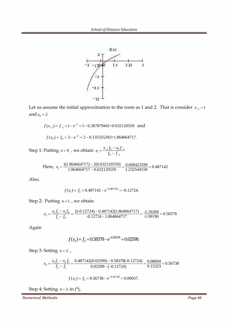
The graph of ( ) xf x x e is as shown here.
School of Distance Education
Numerical Methods Page 48
Let us assume the initial approximation to the roots as 1 and 2. That is consider 1 1x
and 0 2x
11 1( ) 1 1 0.367879441=0.632120559f x f e and
20 0( ) 2 2 0.135335283=1.864664717.f x f e
Step 1: Putting 0n , we obtain 1 0 0 11
0 1
x f x fx
f f
Here, 11(1.864664717) 2(0.632120559) 0.600423599 0.487142.
1.864664717 0.632120559 1.232544158x
Also,
0.4871421 1( ) 0.487142 -0.12724.f x f e
Step 2: Putting 1n , we obtain
0 1 1 02
1 0
2(-0.12724) 0.487142(1.864664717) -1.16284 0.58378-0.12724 1.864664717 -1.99190
x f x fx
f f
Again
0.583782 2( ) 0.58378 0.02599.f x f e
Step 3: Setting 2n ,
1 2 2 1
32 1
0.487142(0.02599) 0.58378(-0.12724) 0.08694 0.567380.153230.02599 -0.12724
x f x fx
f f
0.567383 3( ) 0.56738 0.00037.f x f e
Step 4: Setting 3n in (*),
School of Distance Education
Numerical Methods Page 49
2 3 3 24
3 2
0.58378(0.00037) 0.56738(0.02599) -0.01453 0.56710.00037 0.02599 -0.02562
x f x fx
f f
Approximating to three digits, the root can be considered as 0.567.
Exercises
1. Determine the real root of the equation 1xxe using the secant method. Compareyour result with the true value of 0.567143x .
2. Use the secant method to determine the root, lying between 5 and 8, of the equation2.2 69.x
Objective Type Questions
(a) The Newton-Raphson method formula for finding the square root of a realnumber C from the equation 2 0x C is,
(i) 1 2n
n
xx (ii) 1
3
2n
n
xx (iii) 1
1
2n nn
Cx x
x
(iv) None of these
(b) The next iterative value of the root of 22 3 0x using the Newton-Raphsonmethod, if the initial guess is 2, is
(i) 1.275 (ii) 1.375 (iii) 1.475 (iv) None of these
(c) The next iterative value of the root of 22 3 0x using the secant method, if theinitial guesses are 2 and 3, is
(i) 1 (ii) 1.25 (iii) 1.5 (iv) None of these
(d) In secant method,
(i) 1 11
1
n n n nn
n n
x f x fx
f f
(ii) 1 1
11
n n n nn
n n
x f x fx
f f
(iii) 1 1
11
n n n nn
n n
x f x fx
f f
(iv) None of these
Answers
(a) (iii) 1
1
2n nn
Cx x
x
(b) (ii) 1.375
(c) (iii) 1.5
School of Distance Education
Numerical Methods Page 50
(d) (i) 1 11
1
n n n nn
n n
x f x fx
f f
Theoretical Questions with Answers:
1. What is the difference between bracketing and open method?
Ans: For finding roots of a nonlinear equation 0)( xf , bracketing method requirestwo guesses which contain the exact root. But in open method initial guess of theroot is needed without any condition of bracketing for starting the iterative processto find the solution of an equation.
2. When the Generalized Newton’s methods for solving equations is helpful?
Ans: To solve the find the oot of ( ) 0f x with multiplicity p, the generalizedNewton’s formula is required.
3. What is the importance of Secant method over Newton-Raphson method?
Ans: Newton-Raphson method requires the evaluation of derivatives of thefunction and this is not always possible, particularly in the case of functions arisingin practical problems. In such situations Secant method helps to solve the equationwith an approximation to the derivative.
************
School of Distance Education
Numerical Methods Page 51
4
FINITE DIFFERENCES OPERATORS
For a function y=f(x), it is given that 0 1, ,..., ny y y are the values of the variable ycorresponding to the equidistant arguments, 0 1, ,..., nx x x , where
1 0 2 0 3 0 0, 2 , 3 ,..., nx x h x x h x x h x x nh . In this case, even though Lagrange anddivided difference interpolation polynomials can be used for interpolation, some simplerinterpolation formulas can be derived. For this, we have to be familiar with some finitedifference operators and finite differences, which were introduced by Sir Isaac Newton.Finite differences deal with the changes that take place in the value of a function f(x) dueto finite changes in x. Finite difference operators include, forward difference operator,backward difference operator, shift operator, central difference operator and meanoperator.
Forward difference operator ( ) :
For the values 0 1, ,..., ny y y of a function y=f(x), for the equidistant values 0 1 2, , ,..., nx x x x ,where 1 0 2 0 3 0 0, 2 , 3 ,..., nx x h x x h x x h x x nh , the forward difference operator isdefined on the function f(x) as,
1i i i i if x f x h f x f x f x
That is,
1i i iy y y
Then, in particular
0 0 0 1 0
0 1 0
f x f x h f x f x f x
y y y
1 1 1 2 1
1 2 1
f x f x h f x f x f x
y y y
etc.,
0 1, ,..., ,...iy y y are known as the first forward differences.
The second forward differences are defined as,
School of Distance Education
Numerical Methods Page 52
2
2 1
2
2 2
2
i i i i
i i
i i i i
i i i
i i i
f x f x f x h f x
f x h f x
f x h f x h f x h f x
f x h f x h f x
y y y
In particular,
2 20 2 1 0 0 2 1 02 2f x y y y or y y y y
The third forward differences are,
3 2
2 2
3 33 2 1
f x f xi i
f x h f x h f xi i i
y y y yii i i
In particular,
3 30 3 2 1 0 0 3 2 1 03 3 3 3f x y y y y or y y y y y
In general the nth forward difference,
1 1n n ni i if x f x h f x
The differences 2 30 0 0, , ....y y y are called the leading differences.
Forward differences can be written in a tabular form as follows:
x y y 2 y 3 y
0x
1x
2x
3x
0 ( )oy f x
1 1( )y f x
2 2( )y f x
3 3( )y f x
0 1 0y y y
1 2 1y y y
2 3 2y y y
20 1 0y y y
21 2 1y y y
3 2 20 1 0y y y
School of Distance Education
Numerical Methods Page 53
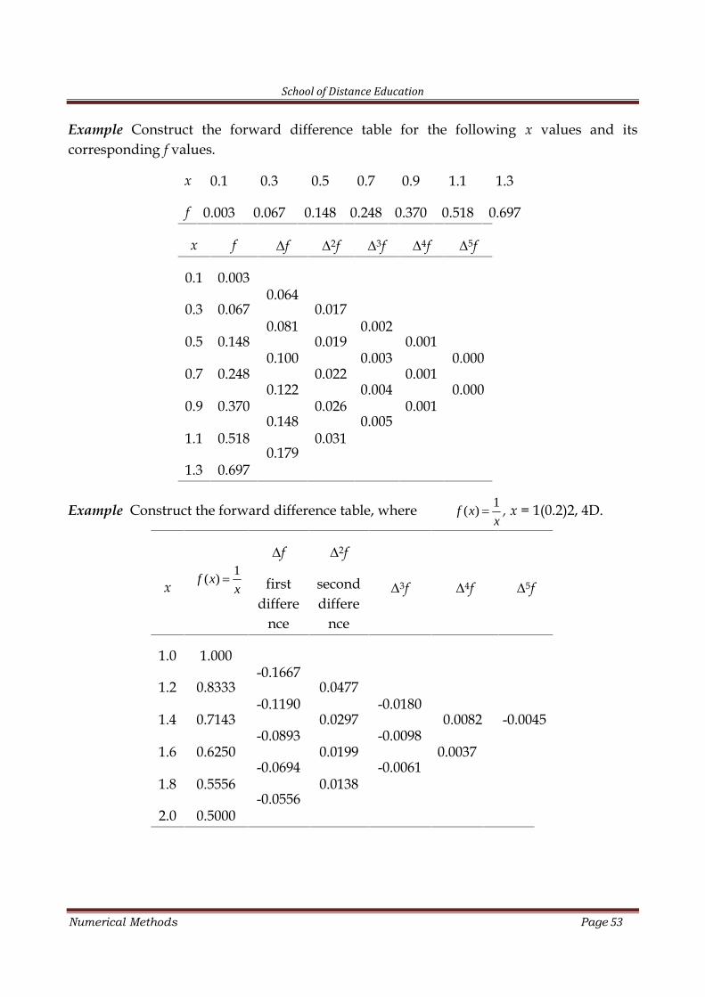
Example Construct the forward difference table for the following x values and itscorresponding f values.
x 0.1 0.3 0.5 0.7 0.9 1.1 1.3
f 0.003 0.067 0.148 0.248 0.370 0.518 0.697
x f f 2f 3f 4f 5f
0.1 0.0030.064
0.081
0.100
0.122
0.148
0.179
0.3 0.067 0.0170.002
0.003
0.004
0.005
0.5 0.148 0.019 0.0010.000
0.0000.7 0.248 0.022 0.001
0.9 0.370 0.026 0.001
1.1 0.518 0.031
1.3 0.697
Example Construct the forward difference table, wherex
xf1
)( , x = 1(0.2)2, 4D.
x xxf
1)(
f
firstdiffere
nce
2f
seconddiffere
nce
3f 4f 5f
1.0 1.000-0.1667
-0.1190
-0.0893
-0.0694
-0.0556
1.2 0.8333 0.0477-0.0180
-0.0098
-0.0061
1.4 0.7143 0.0297 0.0082 -0.0045
1.6 0.6250 0.0199 0.0037
1.8 0.5556 0.0138
2.0 0.5000
School of Distance Education
Numerical Methods Page 54
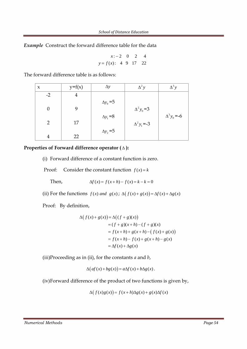
Example Construct the forward difference table for the data
: 2 0 2 4
( ) : 4 9 17 22
x
y f x
The forward difference table is as follows:
x y=f(x) y 2 y 3 y
-2
0
2
4
4
9
17
22
0y =5
1y =8
2y =5
20y =3
21y =-3
30y =-6
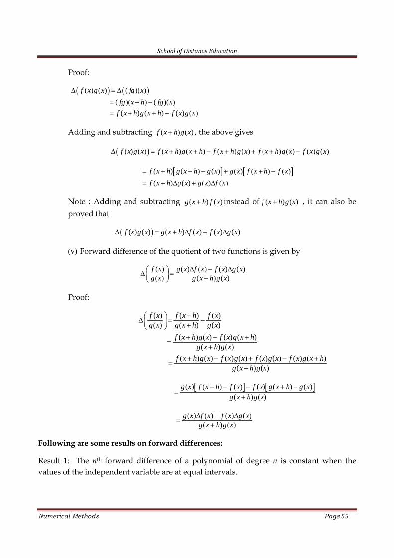
Properties of Forward difference operator ( ):
(i) Forward difference of a constant function is zero.
Proof: Consider the constant function ( )f x k
Then, ( ) ( ) ( ) 0f x f x h f x k k
(ii) For the functions ( ) ( )f x and g x ; ( ) ( ) ( ) ( )f x g x f x g x
Proof: By definition,
( ) ( ) ( )( )
( )( ) ( )( )
( ) ( ) ( ) ( )
( ) ( ) ( ) ( )
( ) ( )
f x g x f g x
f g x h f g x
f x h g x h f x g x
f x h f x g x h g x
f x g x
(iii)Proceeding as in (ii), for the constants a and b,
( ) ( ) ( ) ( )af x bg x a f x b g x .
(iv)Forward difference of the product of two functions is given by,
( ) ( ) ( ) ( ) ( ) ( )f x g x f x h g x g x f x
School of Distance Education
Numerical Methods Page 55
Proof:
( ) ( ) ( )( )
( )( ) ( )( )
( ) ( ) ( ) ( )
f x g x fg x
fg x h fg x
f x h g x h f x g x
Adding and subtracting ( ) ( )f x h g x , the above gives
( ) ( ) ( ) ( ) ( ) ( ) ( ) ( ) ( ) ( )f x g x f x h g x h f x h g x f x h g x f x g x
( ) ( ) ( ) ( ) ( ) ( )
( ) ( ) ( ) ( )
f x h g x h g x g x f x h f x
f x h g x g x f x
Note : Adding and subtracting ( ) ( )g x h f x instead of ( ) ( )f x h g x , it can also beproved that
( ) ( ) ( ) ( ) ( ) ( )f x g x g x h f x f x g x
(v) Forward difference of the quotient of two functions is given by
( ) ( ) ( ) ( ) ( )( ) ( ) ( )
f x g x f x f x g xg x g x h g x
Proof:
( ) ( ) ( )( ) ( ) ( )
( ) ( ) ( ) ( )( ) ( )
( ) ( ) ( ) ( ) ( ) ( ) ( ) ( )( ) ( )
f x f x h f xg x g x h g x
f x h g x f x g x hg x h g x
f x h g x f x g x f x g x f x g x hg x h g x
( ) ( ) ( ) ( ) ( ) ( )( ) ( )
g x f x h f x f x g x h g x
g x h g x
( ) ( ) ( ) ( )( ) ( )
g x f x f x g xg x h g x
Following are some results on forward differences:
Result 1: The nth forward difference of a polynomial of degree n is constant when thevalues of the independent variable are at equal intervals.
School of Distance Education
Numerical Methods Page 56
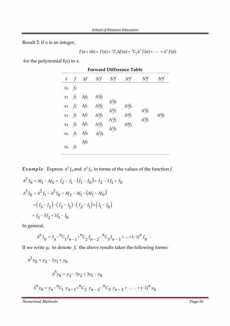
Result 2: If n is an integer,2
1 2( ) ( ) ( ) ( ) ( )n n nf a nh f a C f a C f a f a
for the polynomial f(x) in x.
Forward Difference Table
x f f 2f 3f 4f 5f 6f
x0 f0
f0
f1
f2
f3
f4
f5
x1 f1 2f03f0
3f1
3f2
3f3
x2 f2 2f2 4f05f0
5f1x3 f3 2f2 4f1 6f0
x4 f4 2f3 4f2
x5 f5 2f4
x6 f6
Example Express 02 f and 0
3 f in terms of the values of the function f.
012201120102 ffffffffff
011202
12
03 fffffff
3 2 2 1 2 1 1 0f f f f f f f f
3 33 2 1 0f f f f
In general,
0)1(...
3322110fn
nfCn
nfCn
nfCn
nffn
.
If we write yn to denote fn the above results takes the following forms:
012202 yyyy
01323303 yyyyy
0)1(...3322110 ynnyCn
nyCnnyCn
nyyn
School of Distance Education
Numerical Methods Page 57
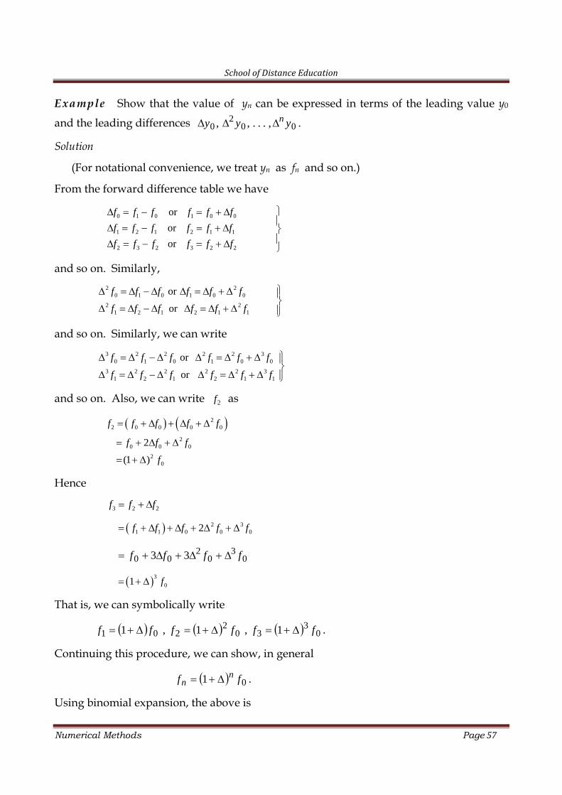
Example Show that the value of yn can be expressed in terms of the leading value y0
and the leading differences .,...,, 002
0 yyy n
Solution
(For notational convenience, we treat yn as fn and so on.)
From the forward difference table we have
0 1 0 1 0 0
1 2 1 2 1 1
2 3 2 3 2 2
or
or
or
f f f f f f
f f f f f f
f f f f f f
and so on. Similarly,2 2
0 1 0 1 0 0
2 21 2 1 2 1 1
or
or
f f f f f f
f f f f f f
and so on. Similarly, we can write3 2 2 2 2 3
0 1 0 1 0 0
3 2 2 2 2 31 2 1 2 1 1
or
or
f f f f f f
f f f f f f
and so on. Also, we can write 2f as
22 0 0 0 0
20 0 0
20
2
(1 )
f f f f f
f f f
f
Hence
3 2 2f f f
2 31 1 0 0 02f f f f f
03
02
00 33 ffff
3 01 f
That is, we can symbolically write
.1,1,1 03
302
201 ffffff
Continuing this procedure, we can show, in general
.1 0ff nn
Using binomial expansion, the above is
School of Distance Education
Numerical Methods Page 58
002
2010 ... ffCfCff nnnn
Thus
00
.n
n in i
i
f C f
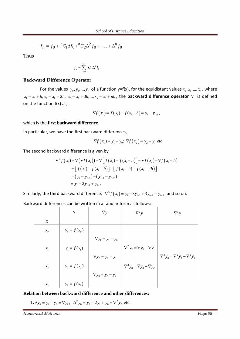
Backward Difference Operator
For the values 0 1, ,..., ny y y of a function y=f(x), for the equidistant values 0 1, ,..., nx x x , where
1 0 2 0 3 0 0, 2 , 3 ,..., nx x h x x h x x h x x nh , the backward difference operator is definedon the function f(x) as,
1) (i i i i if x f x f x h y y ,
which is the first backward difference.
In particular, we have the first backward differences,
1 1 0 2 2 1;f x y y f x y y etc
The second backward difference is given by
2
1 1 2
1 2
) (
) ( ) ( 2
2
i i i i i i
i i i i
i i i i
i i i
f x f x f x f x h f x f x h
f x f x h f x h f x h
y y y y
y y y
Similarly, the third backward difference, 31 2 33 3i i i i if x y y y y and so on.
Backward differences can be written in a tabular form as follows:
x
Y y 2 y 3 y
ox
1x
2x
3x
0 ( )oy f x
1 1( )y f x
2 2( )y f x
3 3( )y f x
1 1 0y y y
2 2 1y y y
3 3 2y y y
22 2 1y y y
23 3 2y y y
3 2 23 3 2y y y
Relation between backward difference and other differences:
1. 0 1 0 1y y y y ; 2 20 2 1 0 22y y y y y etc.
School of Distance Education
Numerical Methods Page 59
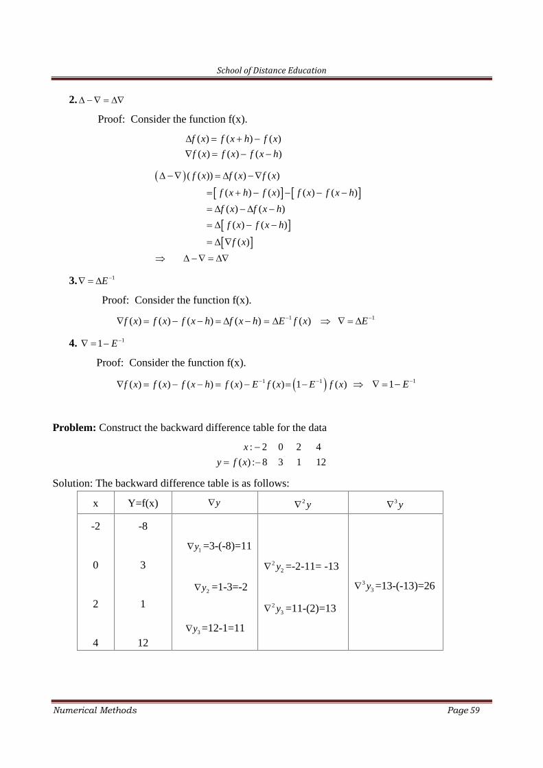
2.
Proof: Consider the function f(x).
( ) ( ) ( )
( ) ( ) ( )
f x f x h f x
f x f x f x h
( ( )) ( ) ( )
( ) ( ) ( ) ( )
( ) ( )
( ) ( )
( )
f x f x f x
f x h f x f x f x h
f x f x h
f x f x h
f x
3. 1E
Proof: Consider the function f(x).
1( ) ( ) ( ) ( ) ( )f x f x f x h f x h E f x 1E
4. 11 E
Proof: Consider the function f(x).
1 1( ) ( ) ( ) ( ) ( ) 1 ( )f x f x f x h f x E f x E f x 11 E
Problem: Construct the backward difference table for the data
: 2 0 2 4
( ) : 8 3 1 12
x
y f x
Solution: The backward difference table is as follows:
x Y=f(x) y 2 y 3 y
-2
0
2
4
-8
3
1
12
1y =3-(-8)=11
2y =1-3=-2
3y =12-1=11
22y =-2-11= -13
23y =11-(2)=13
33y =13-(-13)=26
School of Distance Education
Numerical Methods Page 60
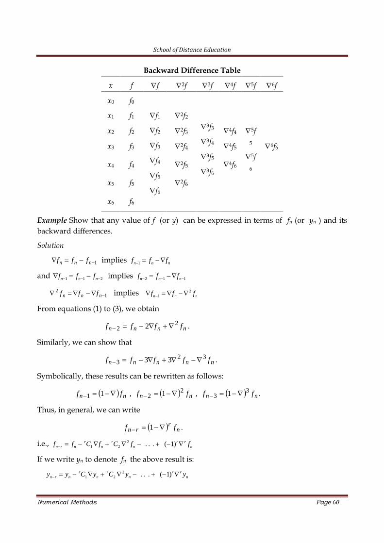
Backward Difference Table
x f f 2f 3f 4f 5f 6f
x0 f0
f1
f2
f3
f4
f5
f6
x1 f1 2f2
3f3
3f4
3f5
3f6
x2 f2 2f3 4f4 5f5
5f6
x3 f3 2f4 4f5 6f6
x4 f4 2f5 4f6
x5 f5 2f6
x6 f6
Example Show that any value of f (or y) can be expressed in terms of fn (or yn ) and itsbackward differences.
Solution
1 nnn fff implies 1n n nf f f
and 1 1 2n n nf f f implies 2 1 1n n nf f f
12
nnn fff implies 21n n nf f f
From equations (1) to (3), we obtain
nnnn ffff 22 2 .
Similarly, we can show that
nnnnn fffff 323 33 .
Symbolically, these results can be rewritten as follows:
.1,1,1 33
221 nnnnnn ffffff
Thus, in general, we can write
nr
rn ff 1 .
i.e., 21 2 . . . ( 1)r r r r
n r n n n nf f C f C f f
If we write yn to denote fn the above result is:2
1 2 . . . ( 1)r r r rn r n n n ny y C y C y y
School of Distance Education
Numerical Methods Page 61
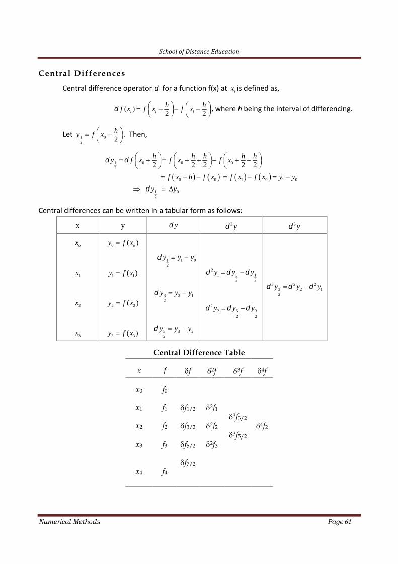
Central Differences
Central difference operator for a function f(x) at ix is defined as,
( )2 2i i ih hf x f x f x
, where h being the interval of differencing.
Let 1 02 2
hy f x
. Then,
1 0 0 02
0 0 1 0 1 0
1 02
2 2 2 2 2h h h h hy f x f x f x
f x h f x f x f x y y
y y
Central differences can be written in a tabular form as follows:
x y y 2 y 3 y
ox
1x
2x
3x
0 ( )oy f x
1 1( )y f x
2 2( )y f x
3 3( )y f x
1 1 02
y y y
3 2 12
y y y
5 3 22
y y y
21 3 1
2 2
y y y
22 5 3
2 2
y y y
3 2 23 2 12
y y y
Central Difference Table
x f f 2f 3f 4f
x0 f0
f1/2
f3/2
f5/2
f7/2
x1 f1 2f13f3/2
3f5/2
x2 f2 2f2 4f2
x3 f3 2f3
x4 f4
School of Distance Education
Numerical Methods Page 62
Example Show that
(a)1
21
2
m
fmfmfmf
(b)1
31
32
2
13
mf
mf
mf
mf
mf
(a) 2 ( ) ( )1 11/2 1/2f f f f f f fm m mm mm m
21 1f f fmm m
(b) 3 2 2 211/2 2 1f f f f f fmmm m m m
21 1
f f fm m m 1
31
32
m
fm
fm
fm
f
Shift operator, E
Let y = f (x) be a function of x, and let x takes the consecutive values x, x + h, x + 2h, etc.We then define an operator E, called the shift operator having the property
E f(x) = f (x + h) …(1)
Thus, when E operates on f (x), the result is the next value of the function. If we apply theoperator twice on f (x), we get
E2 f (x) = E [E f (x)] = f (x+ 2h).
Thus, in general, if we apply the shift operator n times on f (x), we arrive at
E n f (x) = f (x+ nh) …(2)
for all real values of n.
If f0 (= y0), f1 (= y1)… are the consecutive values of the function
y = f (x), then we can also write
E f0 = f1 (or E y0 = y1), E f1 = f2 (or E y1 = y2)…
E2f0 = f2 (or E 2y0 = y2), E 2 f1 = f3 (or E y1 = y3)…
E3f0 = f3 (or E 2y0 = y3), E 3 f1 = f4 (or E y1 = y4)…
and so on. The inverse operator E1 is defined as:
School of Distance Education
Numerical Methods Page 63
E1 f(x) = f (x h) …(3)
and similarly
En f(x) = f (x nh) …(4)
Average Operator
The average operator is defined as
2 21 ( ) ( )2
h hf x f x f x
Differential operator D
The differential operator D has the property
( ) ( ) ( )dDf x f x f xdx
22
2( ) ( ) ( )dD f x f x f x
dx
Relations between the operators:
Operators,,, and D in terms of E
From the definition of operators and E, we have
f (x) = f (x + h) f (x) = E f (x) f (x) = (E 1) f (x).
Therefore,
= E 1
From the definition of operators and E 1, we have
f (x) = f (x) f (x h) = f (x) E 1f (x) = (1 E 1) f (x).
Therefore,
1 11 .EEE
The definition of the operators and E gives
f (x) = f (x + h/2) f (x h/2) = E 1/2f (x) E 1/2f (x)
= (E 1/2 E 1/2) f (x).
School of Distance Education
Numerical Methods Page 64
Therefore,
= E 1/2 E 1/2
The definition of the operators and E yields
1/ 2 1/ 21 1 .2 2 2 2
h hf x f x f x E E f x
Therefore,
1/ 2 1/ 21 .2
E E
It is known that
E f (x) = f (x + h).
Using the Taylor series expansion, we have
2
. . .2!hEf x f x h f x f x
2
2 . . .2!hf x h Df x D x
2 2
1 . . .1! 2!
hDh D h D f x e f x
.
Thus hDeE . Or,
hD = log E.
Example If , , denote forward, backward and central difference operators, E and respectively the shift operator and average operators, in the analysis of data with equalspacing h, prove the following:
222 2 1/ 2
22
( ) 1 12 2
1 / 42
i ii E
iii
1
.2 2 2Eiv v
Solution
(i) From the definition of operators, we have
School of Distance Education
Numerical Methods Page 65
1/ 2 1/ 2 1/ 2 1/ 2 11 12 2
E E E E E E .
Therefore
22 2 2 2 11 11 1 24 4
E E E E
Also,
2 21/ 2 1/ 2 11 11 1
2 2 2E E E E
From equations (1) and (2), we get22
2 21 1 .2
(ii) 1/ 2 1/ 2 1/ 2 1/ 2 1/ 21 .2 2
E E E E E
(iii) We can write
21/ 2 1/ 2221 / 4
2 2
E E 21/ 2 1/ 2 1/ 2 1/ 2114
E E E E
1
1/ 2 1/ 2 1/ 2 1/ 22 12 2
E E E E E E
1 122 2
E E E E
= E 1
=
(iv) We write
1/ 2 1/ 2 1/ 2 1/ 2 11 12 2
E E E E E E
1 11 1 1 11 1 .2 2 2 2 2 2 2
EE EE E
(v) We can write
1/ 2 1/ 2 1/ 2 1/ 2 11 12 2
E E E E E E
1 11 1 .2 2
School of Distance Education
Numerical Methods Page 66
Example Prove that
1log 1 log 1 sinh .hD
Using the standard relations given in boxes in the last section, we have
1log log 1 log log log 1hD E E E
Also,
1/ 2 1/ 2 1/ 2 1/ 2 11 12 2
E E E E E E
1 sin2
hD hDe e hD
Therefore
.sinh 1 hD
Example Show that the operations and E commute.
Solution
From the definition of operators and E , we have
0 1 3/ 2 1/ 212
Ef f f f
and also
0 1/ 2 1/ 2 3/ 2 1/ 21 12 2
E f E f f f f
Hence
.E E
Therefore, the operators and E commute.
Example Show that2 2
20 0 0 0 1 2... ...
2! 2!
x x xe u x u u u u x u
2 2 22
0 0 0 0... 1 ...2! 2!
x xx xe u x u u e x u
(1 )0 0
x x xe e u e u
0 xEe u
School of Distance Education
Numerical Methods Page 67
2 2
01 ...2!
x ExE u
2
0 1 2 ...,2!
xu xu u
as desired.
Example Using the method of separation of symbols, show that
1 2
( 1)( 1) .
2 n n
x n x x x x n
n nu u nu u u
To prove this result, we start with the right-hand side. Thus,
R.H.S 1 2
( 1)( 1) .
2 n
x x x x n
n nu nu u u
1 2( 1)( 1)
2 n n
x x x x
n nu nE u E u E u
1 2( 1)1 ( 1)
2
n nx
n nnE E E u
11 n
xE u
11
n
xuE
1
n
xE u
E
n
xn uE
n nxE u
, nx nu
= L.H.S
Differences of a Polynomial
Let us consider the polynomial of degree n in the form1 2
0 1 2 1( ) . . . ,n n nn nf x a x a x a x a x a
where 0 0a and 0 1 2 1, , , . . . , ,n na a a a a are constants. Let h be the interval of differencing.Then
School of Distance Education
Numerical Methods Page 68
1 20 1 2( ) ( ) ( ) ( ) ...n n nf x h a x h a x h a x h 1( )n na x h a
Now the difference of the polynomials is:
1 10 1( ) ( ) ( ) ( ) ( ) ...n n n nf x f x h f x a x h x a x h x 1( )na x h x
Binomial expansion yields
nnnnnnn xhhxChxCxaxf ...222
110
1 11 2 3 21 1 2[ n nn n na x C x h C x h
1 11. . . ] . . .n n
nh x a h
.... 12
11
12
201
0 haxhCahCanhxa nnnnn
Therefore,
,...3210 lxkxcxbnhxaxf nnn
where b, c, . . . , k, l are constants involving h but not x. Thus, the first difference ofa polynomial of degree n is another polynomial of degree (n 1). Similarly,
xfhxfxfxf 2
1 21 20
n nn na nh x h x b x h x
. . . k x h x
On simplification, it reduces to the form
qxcxbxhnnaxf nnn ...1 43220
2 .
Therefore, xf2 is a polynomial of degree (n 2) in x. Similarly, we can form thehigher order differences, and every time we observe that the degree of the polynomial isreduced by 1. After differencing n times, we are left with only the first term in form
0 1 2 3 . . . 2 1n nf x a n n n n h
0 ! constant.na n h
This constant is independent of x. Since xfn is a constant .01 xfn Hence the (n+ 1)th and higher order differences of a polynomial of degree n are 0.
School of Distance Education
Numerical Methods Page 69
Conversely, if the n th differences of a tabulated function are constant and the ( 1)thn ,( 2)th,...,n differences all vanish, then the tabulated function represents a polynomial ofdegree n. It should be noted that these results hold good only if the values of x are equallyspaced. The converse is important in numerical analysis since it enables us to approximatea function by a polynomial if its differences of some order become nearly constant.
Theorem (Differences of a polynomial)The nth differences of a polynomial of degree n is aconstant, when the values of the independent variable are given at equal intervals.
Exercises
1. Calculate 1)2.0(0,1
1)(
x
xxf to (a) 2 decimal places, (b) 3 decimal places and (c)4
decimal places. Then compare the effect of rounding errors in the correspondingdifference tables.
2. Express 2y1 (i.e. 2f1 ) and 4y0 (i.e. 4f0 ) in terms of the values of the function y =f(x).
3. Set up a difference table of 2( )f x x for 0(1)10x . Do the same with the calculatedvalue 25 of (5)f replaced by 26. Observe the spread of the error.
4. Calculate 1)2.0(0,1
1)(
x
xxf to (a)2 decimal places, (b)3 decimal places and (c)4
decimal places. Then compare the effect of rounding errors in the correspondingdifference tables.
5. Set up a forward difference table of f(x) = x2 for x = 0(1)10. Do the same with thecalculated value 25 of f(5) replaced by 26. Observe the spread of the error.
6. Construct the difference table based on the following table.
x 0.0 0.1 0.2 0.3 0.4 0.5
cosx 1.000 00 0.995 00 0.980 07 0.955 34 0.921 06 0.877 58
7. Construct the difference table based on the following table.
x 0.0 0.1 0.2 0.3 0.4 0.5
sinx 0.000 00 0.09983
0.19867
0.29552
0.38942
0.479
8. Construct the backward difference table, where
( ) sinf x x , x = 1.0(0.1)1.5, 4D.
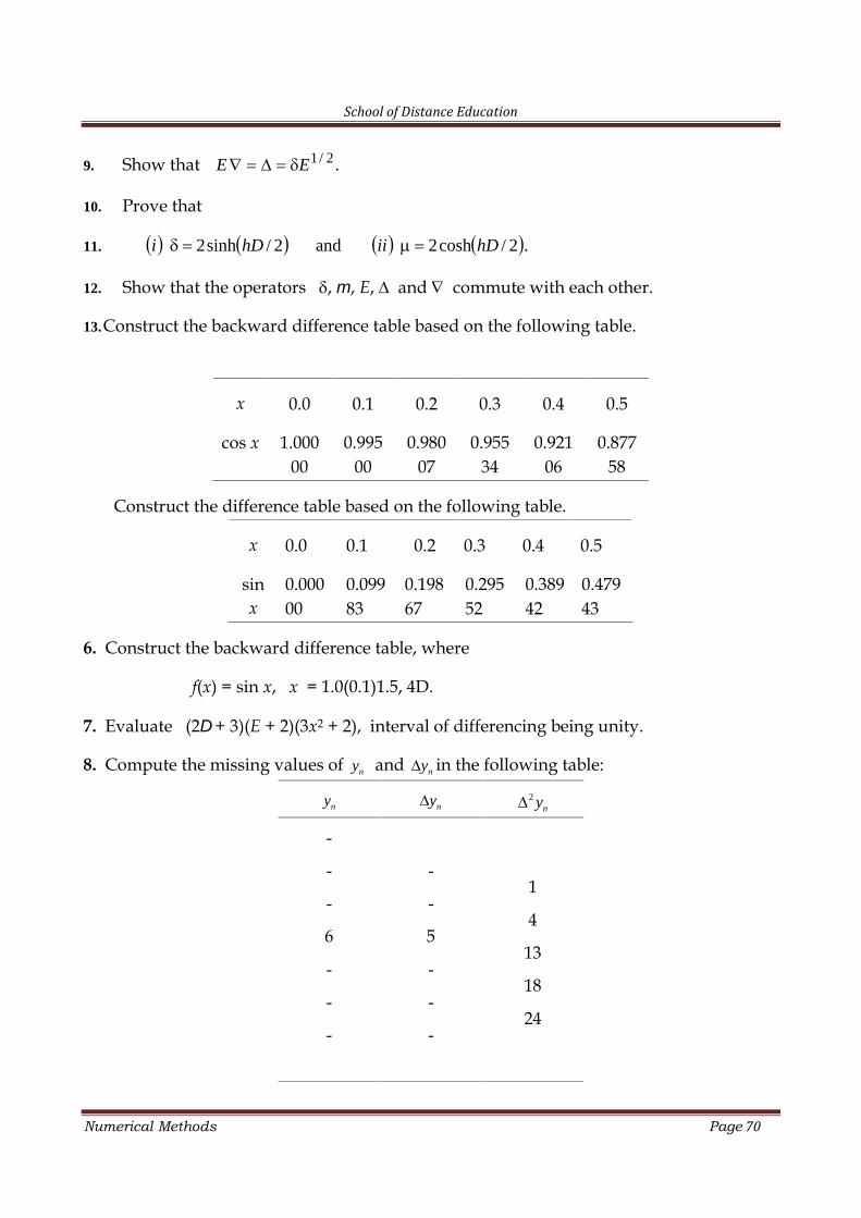
School of Distance Education
Numerical Methods Page 70
9. Show that .2/1EE
10. Prove that
11. .2/cosh2and2/sinh2 hDiihDi
12. Show that the operators , , E, and commute with each other.
13.Construct the backward difference table based on the following table.
x 0.0 0.1 0.2 0.3 0.4 0.5
cos x 1.00000
0.99500
0.98007
0.95534
0.92106
0.87758
Construct the difference table based on the following table.
x 0.0 0.1 0.2 0.3 0.4 0.5
sinx
0.00000
0.09983
0.19867
0.29552
0.38942
0.47943
6. Construct the backward difference table, where
f(x) = sin x, x = 1.0(0.1)1.5, 4D.
7. Evaluate (2 + 3)(E + 2)(3x2 + 2), interval of differencing being unity.
8. Compute the missing values of ny and ny in the following table:
ny ny 2ny
-
-
-
5
-
-
-
1
4
13
18
24
-
-
6
-
-
-
School of Distance Education
Numerical Methods Page 71
5
NUMERICAL INTERPOLATION
Consider a single valued continuous function ( )y f x defined over [a,b] where( )f x is known explicitly. It is easy to find the values of ‘y’ for a given set of values of ‘x’ in
[a,b]. i.e., it is possible to get information of all the points ( , )x y where .a x b
But the converse is not so easy. That is, using only the points 0 0( , )x y , 1 1( , )x y ,…,( , )n nx y where , 0,1,2,...,ia x b i n , it is not so easy to find the relation between x and y inthe form ( )y f x explicitly. That is one of the problem we face in numericaldifferentiation or integration.
Now we have first to find a simpler function, say ( )g x , such that ( )f x and ( )g x agreeat the given set of points and accept the value of ( )g x as the required value of ( )f x at somepoint x in between a and b. Such a process is called interpolation. If ( )g x is apolynomial, then the process is called polynomial interpolation.
When a function f(x) is not given explicitly and only values of ( )f x are given at aset of distinct points called nodes or tabular points, using the interpolated function ( )g x tothe function f(x), the required operations intended for ( )f x , like determination of roots,differentiation and integration etc. can be carried out. The approximating polynomial ( )g x
can be used to predict the value of ( )f x at a non- tabular point. The deviation of ( )g x from( )f x , that is ( ) ( )f x g x is called the error of approximation.
Consider a continuous single valued function ( )f x defined on an interval [a, b].Given the values of the function for n + 1 distinct tabular points 0 1, ,..., nx x x such that
0 1 ... na x x x b . The problem of polynomial interpolation is to find a polynomial g(x)or ( )np x , of degree n, which fits the given data. The interpolation polynomial fitted to agiven data is unique.
If we are given two points satisfying the function such as 0 0 1 1, ; ,x y x y , where
0 0y f x and 1 1y f x it is possible to fit a unique polynomial of degree 1. If threedistinct points are given, a polynomial of degree not greater than two can be fitteduniquely. In general, if n+ 1 distinct points are given, a polynomial of degree not greaterthan n can be fitted uniquely.
Interpolation fits a real function to discrete data. Given the set of tabular values
0 0 1 1( , ), ( , ) ( , ) n nx y x y x y satisfying the relation ( )y f x , where the explicit nature of
School of Distance Education
Numerical Methods Page 72
( )f x is not known, and it is required to find the values of ( )f x corresponding to certaingiven values of x in between x0 and xn . To do this we have first to find a simpler function,say ( )g x , such that ( )f x and ( )g x agree at the set of tabulated points and accept the valueof ( )g x as the required value of ( )f x at some point x in between x0 and xn . Such a processis called interpolation. If ( )g x is a polynomial, then the process is called polynomialinterpolation.
In interpolation, we have to determine the function ( )g x , in the case that ( )f x isdifficult to be obtained, using the pivotal values 0 0( ),f f x 1 1( )f f x ,. . . , ( )n nf f x .
Linear interpolation
In linear interpolation, we are given with two pivotal values 0 0( )f f x and 1 1( ),f f x
and we approximate the curve of f by a chord (straight line) P1 passing through the points0 0( , )x f and 1 1( , )x f . Hence the approximate value of f at the intermediate point 0x x rh
is given by the linear interpolation formula
1 0 1 0 0 0( ) ( ) ( )f x P x f r f f f r f
where 0x x
rh
and 10 r .
Example Evaluate ln 9.2 , given that ln 9.0 2.197 and ln 9.5 2.251.
Here x0 = 9.0 , x1 = 9.5, h = x1 x0 =9.5 9.0 = 0.5, f0 = f(x0) = ln 9.0 2.197 and1 1( ) ln 9.5 2.251. f f x Now to calculate ln9.2 (9.2), f take 9.2,x so that
0 9.2 9.0 0.2 0.40.5 0.5
x xr
h
and hence
1 0 1 0ln 9.2 (9.2) (9.2) ( ) 2.197 0.4 (2.251 2.197) 2.219f P f r f f
Example Evaluate f (15), given that f(10) = 46, f(20) = 66.
Here x0 = 10 , x1 = 20, h = x1 x0 =20 10 = 10,
f0 = f(x0) = 46 and f1 = f(x1) = 66.
Now to calculate f(15), take x = 15, so that
0 15 10 5 0.510 10
x xr
h
and hence1 0 1 0
(15) (15) ( ) 46 0.5 (66 46) 56f P f r f f
Example Evaluate 1.24e , given that 1.1
3.0042e and 1.44.0552e .
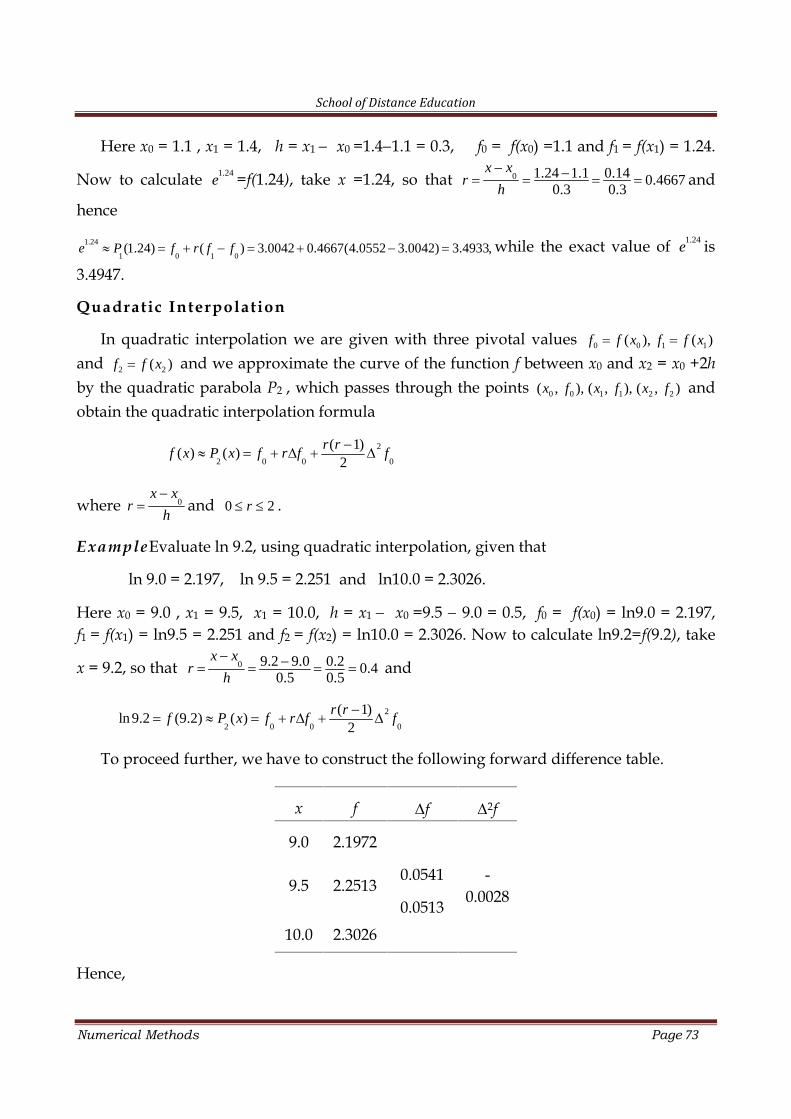
School of Distance Education
Numerical Methods Page 73
Here x0 = 1.1 , x1 = 1.4, h = x1 x0 =1.41.1 = 0.3, f0 = f(x0) =1.1 and f1 = f(x1) = 1.24.
Now to calculate 1.24e =f(1.24), take x =1.24, so that 0 1.24 1.1 0.14 0.4667
0.3 0.3
x xr
h
and
hence
1.24
1 0 1 0(1.24) ( ) 3.0042 0.4667(4.0552 3.0042) 3.4933,e P f r f f while the exact value of 1.24
e is
3.4947.
Quadratic Interpolation
In quadratic interpolation we are given with three pivotal values 0 0 1 1( ), ( ) f f x f f x
and 2 2( )f f x and we approximate the curve of the function f between x0 and x2 = x0 +2hby the quadratic parabola P2 , which passes through the points 0 0 1 1 2 2( , ), ( , ), ( , )x f x f x f andobtain the quadratic interpolation formula
2
2 0 0 0
( 1)( ) ( )
2r r
f x P x f r f f
where 0x x
rh
and 20 r .
ExampleEvaluate ln 9.2, using quadratic interpolation, given that
ln 9.0 = 2.197, ln 9.5 = 2.251 and ln10.0 = 2.3026.
Here x0 = 9.0 , x1 = 9.5, x1 = 10.0, h = x1 x0 =9.5 9.0 = 0.5, f0 = f(x0) = ln9.0 = 2.197,f1 = f(x1) = ln9.5 = 2.251 and f2 = f(x2) = ln10.0 = 2.3026. Now to calculate ln9.2=f(9.2), take
x = 9.2, so that 0 9.2 9.0 0.2 0.40.5 0.5
x xr
h
and
2
2 0 0 0
( 1)ln 9.2 (9.2) ( )
2r r
f P x f r f f
To proceed further, we have to construct the following forward difference table.
x f f 2f
9.0 2.1972
0.0541
0.05139.5 2.2513
-0.0028
10.0 2.3026
Hence,
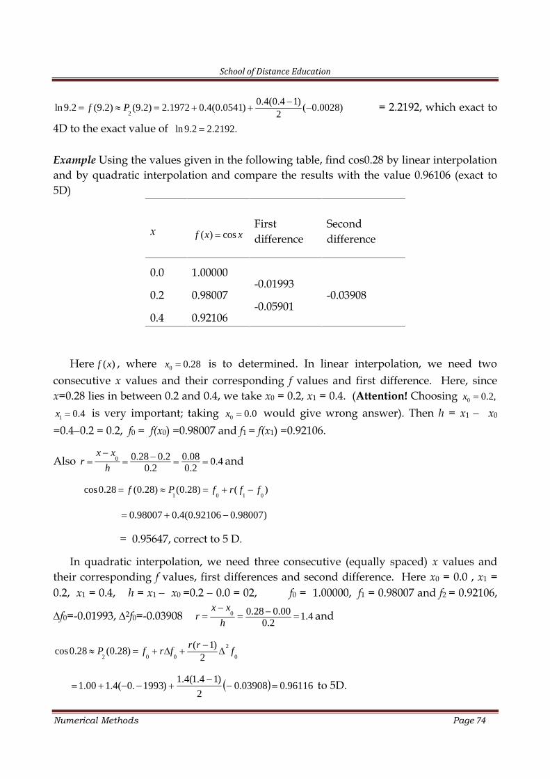
School of Distance Education
Numerical Methods Page 74
2
0.4(0.4 1)ln 9.2 (9.2) (9.2) 2.1972 0.4(0.0541) ( 0.0028)
2f P
= 2.2192, which exact to
4D to the exact value of ln 9.2 2.2192.
Example Using the values given in the following table, find cos0.28 by linear interpolationand by quadratic interpolation and compare the results with the value 0.96106 (exact to5D)
x ( ) cosf x xFirstdifference
Seconddifference
0.0 1.00000-0.01993
-0.059010.2 0.98007 -0.03908
0.4 0.92106
Here ( )f x , where 0 0.28x is to determined. In linear interpolation, we need twoconsecutive x values and their corresponding f values and first difference. Here, sincex=0.28 lies in between 0.2 and 0.4, we take x0 = 0.2, x1 = 0.4. (Attention! Choosing 0 0.2,x
1 0.4x is very important; taking 0 0.0x would give wrong answer). Then h = x1 x0
=0.40.2 = 0.2, f0 = f(x0) =0.98007 and f1 = f(x1) =0.92106.
Also 0 0.28 0.2 0.08 0.40.2 0.2
x xr
h
and
1 0 1 0cos0.28 (0.28) (0.28) ( ) f P f r f f
0.98007 0.4(0.92106 0.98007)
= 0.95647, correct to 5 D.
In quadratic interpolation, we need three consecutive (equally spaced) x values andtheir corresponding f values, first differences and second difference. Here x0 = 0.0 , x1 =0.2, x1 = 0.4, h = x1 x0 =0.2 0.0 = 02, f0 = 1.00000, f1 = 0.98007 and f2 = 0.92106,
f0=-0.01993, 2f0=-0.03908 0 0.28 0.00 1.40.2
x xr
h
and
2
2 0 0 0
( 1)cos0.28 (0.28)
2r r
P f r f f
96116.003908.02
)14.1(4.1)1993.0(4.100.1
to 5D.
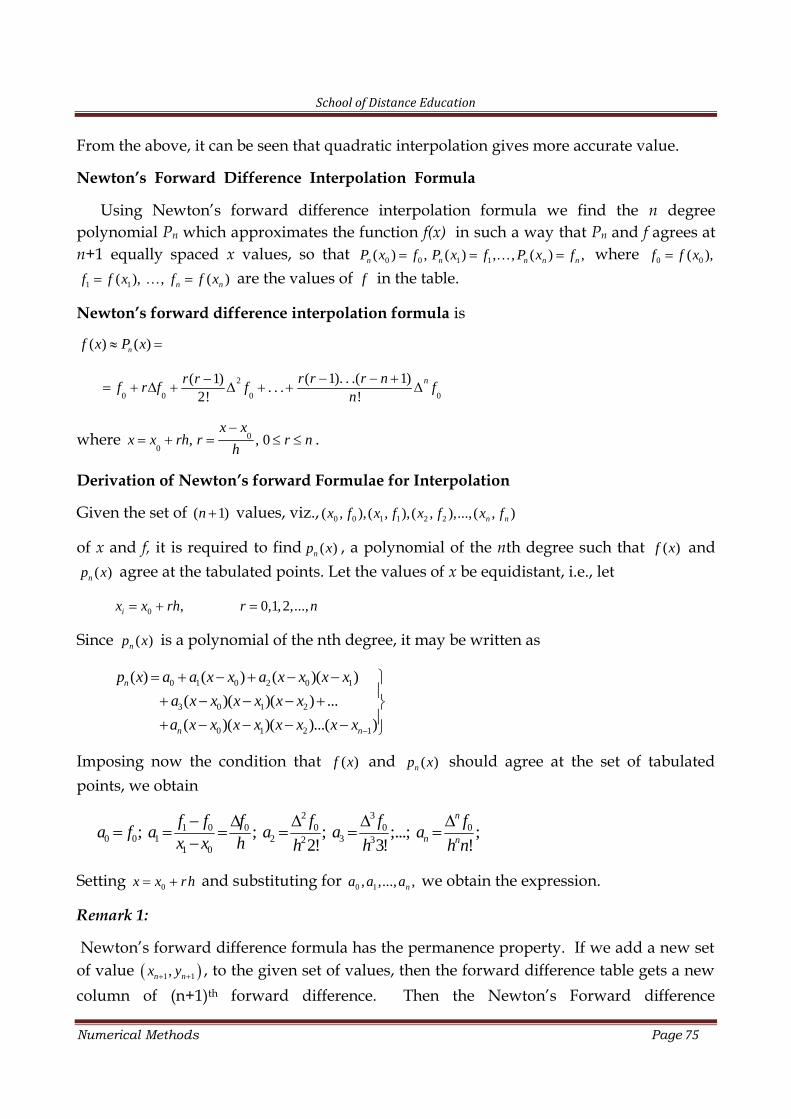
School of Distance Education
Numerical Methods Page 75
From the above, it can be seen that quadratic interpolation gives more accurate value.
Newton’s Forward Difference Interpolation Formula
Using Newton’s forward difference interpolation formula we find the n degreepolynomial Pn which approximates the function f(x) in such a way that Pn and f agrees atn+1 equally spaced x values, so that 0 0 1 1( ) , ( ) , , ( ) , n n n n nP x f P x f P x f where 0 0( ),f f x
1 1( ), , ( ) n nf f x f f x are the values of f in the table.
Newton’s forward difference interpolation formula is
( ) ( )nf x P x
2
0 0 0 0
( 1). . .( 1)( 1). . .
2! !nr r r nr r
f r f f fn
where 0
0, , 0
x xx x rh r r n
h
.
Derivation of Newton’s forward Formulae for Interpolation
Given the set of ( 1)n values, viz., 0 0 1 1 2 2( , ), ( , ), ( , ),..., ( , )n nx f x f x f x f
of x and f, it is required to find ( )np x , a polynomial of the nth degree such that ( )f x and( )np x agree at the tabulated points. Let the values of x be equidistant, i.e., let
0 , 0,1,2,...,ix x rh r n
Since ( )np x is a polynomial of the nth degree, it may be written as
0 1 0 2 0 1
3 0 1 2
0 1 2 1
( ) ( ) ( )( )
( )( )( ) ...
( )( )( )...( )
n
n n
p x a a x x a x x x x
a x x x x x x
a x x x x x x x x
Imposing now the condition that ( )f x and ( )np x should agree at the set of tabulatedpoints, we obtain
2 31 0 0 0 0 0
0 0 1 2 32 31 0
; ; ; ;...; ;2! 3! !
n
n n
f f f f f fa f a a a a
x x h h h h n
Setting 0x x rh and substituting for 0 1, ,..., ,na a a we obtain the expression.
Remark 1:
Newton’s forward difference formula has the permanence property. If we add a new setof value 1 1,n nx y , to the given set of values, then the forward difference table gets a newcolumn of (n+1)th forward difference. Then the Newton’s Forward difference
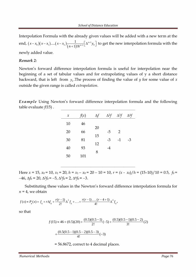
School of Distance Education
Numerical Methods Page 76
Interpolation Formula with the already given values will be added with a new term at the
end, 1
0 1 01
1.....1 !
nn n
x x x x x x yn h
to get the new interpolation formula with the
newly added value.
Remark 2:
Newton’s forward difference interpolation formula is useful for interpolation near thebeginning of a set of tabular values and for extrapolating values of y a short distancebackward, that is left from 0y .The process of finding the value of y for some value of xoutside the given range is called extrapolation.
Example Using Newton’s forward difference interpolation formula and the followingtable evaluate f(15) .
x f(x) f 2f 3f 4f
10 4620
15
12
8
20 66 -5
-3
-4
2
30 81 -1 -3
40 93
50 101
Here x = 15, x0 = 10, x1 = 20, h = x1 x0 = 20 10 = 10, r = (x x0)/h = (15–10)/10 = 0.5, f0 =46, f0 = 20, 2f0 = 5, 3f0 = 2, 4f0 = 3.
Substituting these values in the Newton’s forward difference interpolation formula forn = 4, we obtain
2 4
4 0 0 0 0
( 1) . . . ( 4 1)( 1)( ) ( ) . . .
2! 4!r r rr r
f x P x f r f f f ,
so that
(0.5)(0.5 1) (0.5)(0.5 1)(0.5 2)(15) 46 (0.5)(20) ( 5) (2)
2! 3!f
(0.5(0.5 1)(0.5 2)(0.5 3)( 3)
4!
= 56.8672, correct to 4 decimal places.
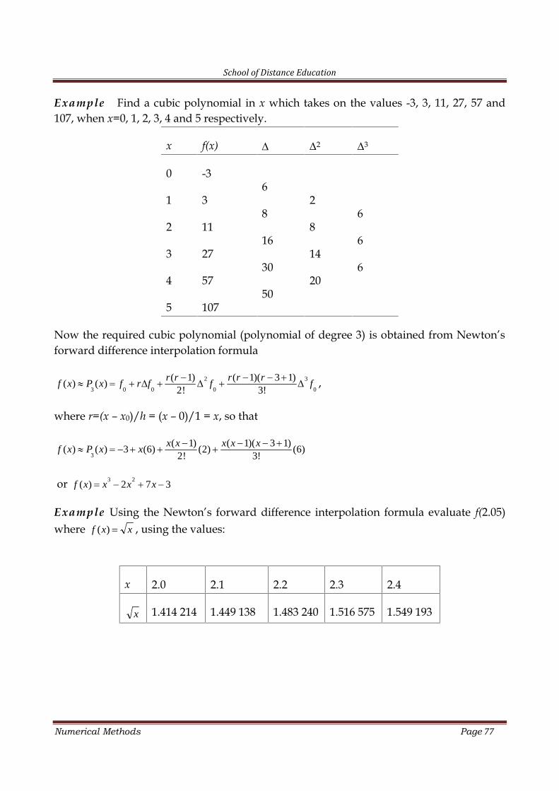
School of Distance Education
Numerical Methods Page 77
Example Find a cubic polynomial in x which takes on the values -3, 3, 11, 27, 57 and107, when x=0, 1, 2, 3, 4 and 5 respectively.
x f(x) 2 3
0 -36
8
16
30
50
1 3 2
8
14
20
6
6
6
2 11
3 27
4 57
5 107
Now the required cubic polynomial (polynomial of degree 3) is obtained from Newton’sforward difference interpolation formula
2 3
3 0 0 0 0
( 1) ( 1)( 3 1)( ) ( )
2! 3!r r r r r
f x P x f r f f f ,
where r=(x – x0)/h = (x – 0)/1 = x, so that
3
( 1) ( 1)( 3 1)( ) ( ) 3 (6) (2) (6)
2! 3!x x x x x
f x P x x
or 3 2( ) 2 7 3f x x x x
Example Using the Newton’s forward difference interpolation formula evaluate f(2.05)where xxf )( , using the values:
x 2.0 2.1 2.2 2.3 2.4
x 1.414 214 1.449 138 1.483 240 1.516 575 1.549 193
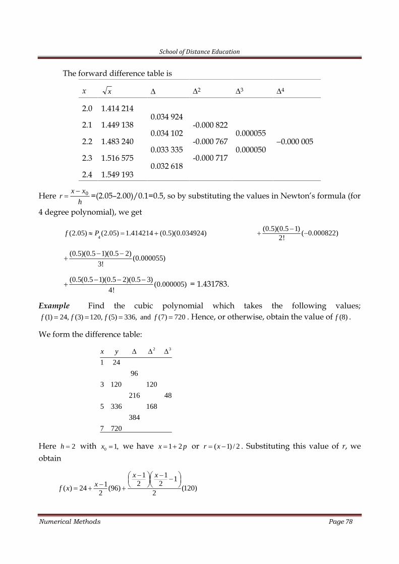
School of Distance Education
Numerical Methods Page 78
The forward difference table is
x x 2 3 4
2.0 1.414 2140.034 924
0.034 102
0.033 335
0.032 618
2.1 1.449 138 -0.000 822
-0.000 767
-0.000 717
0.000055
0.0000502.2 1.483 240 0.000 005
2.3 1.516 575
2.4 1.549 193
Hereh
xxr 0 =(2.05–2.00)/0.1=0.5, so by substituting the values in Newton’s formula (for
4 degree polynomial), we get
4(2.05) (2.05) 1.414214 (0.5)(0.034924)f P
(0.5)(0.5 1)( 0.000822)
2!
(0.5)(0.5 1)(0.5 2)(0.000055)
3!
(0.5(0.5 1)(0.5 2)(0.5 3)(0.000005)
4!
= 1.431783.
Example Find the cubic polynomial which takes the following values;(1) 24, (3) 120, (5) 336, and (7) 720 f f f f . Hence, or otherwise, obtain the value of (8)f .
We form the difference table:2 3
1 24
96
3 120 120
216 48
5 336 168
384
7 720
x y
Here 2h with 0 1,x we have 1 2 x p or ( 1) / 2r x . Substituting this value of r, weobtain
1 1 12 21( ) 24 (96) (120)
2 2
x xxf x
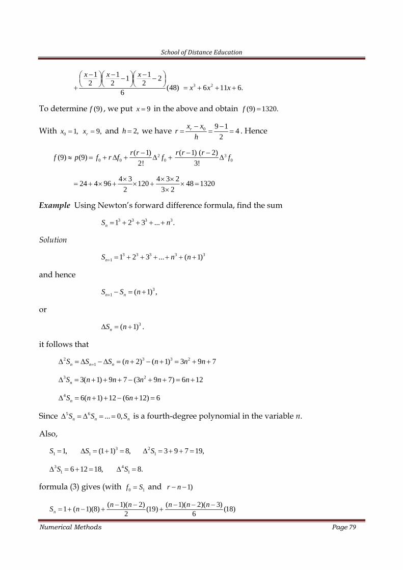
School of Distance Education
Numerical Methods Page 79
1 1 11 22 2 2
(48)6
x x x 3 26 11 6. x x x
To determine (9)f , we put 9x in the above and obtain (9) 1320.f
With 0 1,x 9,rx and 2,h we have 0 9 14
2rx x
rh
. Hence
20 0 0
( 1)(9) (9)
2!
r rf p f r f f
3
0
( 1) ( 2)
3!
r r rf
4 3 4 3 224 4 96 120 48 1320
2 3 2
Example Using Newton’s forward difference formula, find the sum3 3 3 31 2 3 ... . nS n
Solution3 3 3 3 3
1 1 2 3 ... ( 1) nS n n
and hence3
1 ( 1) , n nS S n
or3( 1) nS n .
it follows that2 3 3 2
1 ( 2) ( 1) 3 9 7 n n nS S S n n n n
3 23( 1) 9 7 (3 9 7) 6 12 nS n n n n n
4 6( 1) 12 (6 12) 6 nS n n
Since 5 6 ... 0, n n nS S S is a fourth-degree polynomial in the variable n.
Also,3 2
1 1 11, (1 1) 8, 3 9 7 19,S S S
3 41 16 12 18, 8.S S
formula (3) gives (with 0 1f S and 1)r n
( 1)( 2) ( 1)( 2)( 3)1 ( 1)(8) (19) (18)
2 6 n
n n n n nS n
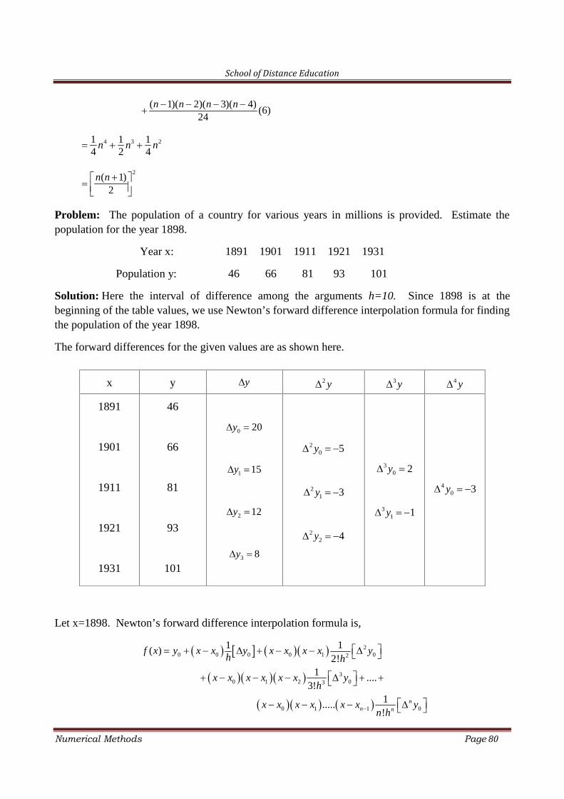
School of Distance Education
Numerical Methods Page 80
( 1)( 2)( 3)( 4)(6)
24 n n n n
4 3 21 1 14 2 4 n n n
2( 1)
2
n n
Problem: The population of a country for various years in millions is provided. Estimate thepopulation for the year 1898.
Year x: 1891 1901 1911 1921 1931
Population y: 46 66 81 93 101
Solution: Here the interval of difference among the arguments h=10. Since 1898 is at thebeginning of the table values, we use Newton’s forward difference interpolation formula for findingthe population of the year 1898.
The forward differences for the given values are as shown here.
Let x=1898. Newton’s forward difference interpolation formula is,
20 0 0 0 1 02
30 1 2 03
0 1 1 0
1 1( )2!
1 ....3!
1.....!
nn n
f x y x x y x x x x yh h
x x x x x x yh
x x x x x x yn h
x y y 2 y 3 y 4 y
1891
1901
1911
1921
1931
46
66
81
93
101
0 20y
1 15y
2 12y
3 8y
20 5y
21 3y
22 4y
30 2y
31 1y
40 3y
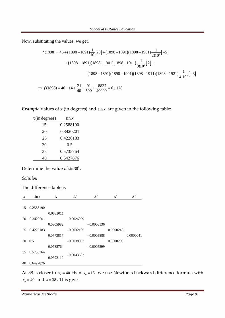
School of Distance Education
Numerical Methods Page 81
Now, substituting the values, we get,
2
3
4
1 1(1898) 46 1898 1891 20 1898 1891 1898 1901 510 2!10
11898 1891 1898 1901 1898 1911 23!10
11898 1891 1898 1901 1898 1911 1898 1921 34!10
f
21 91 18837(1898) 46 14 61.17840 500 40000
f
Example Values of x (in degrees) and sin x are given in the following table:
(in degrees) sin
15 0.2588190
20 0.3420201
25 0.4226183
30 0.5
35 0.5735764
40 0.6427876
x x
Determine the value of 0sin38 .
Solution
The difference table is2 3 4 5sin
15 0.2588190
0.0832011
20 0.3420201 0.0026029
0.0805982 0.0006136
25 0.4226183 0.0032165 0.0000248
0.0773817 0.0005888 0.0000041
30 0.5 0.0038053 0.0000289
0.0735764 0.00
35 0.57357640.0043652
0.0692112
x x
05599
40 0.6427876
As 38 is closer to 40nx than 0 15,x we use Newton’s backward difference formula with40nx and 38x . This gives
School of Distance Education
Numerical Methods Page 82
38 40 2 0.45 5
nx xr
h
Hence, using formula, we obtain
0.4( 0.4 1)(38) 0.6427876 0.4(0.0692112) ( 0.0043652)
2f
( 0.4)( 0.4 1)( 0.4 2)( 0.0005599)
6
( 0.4)( 0.4 1)( 0.4 2)( 0.4 3)(0.0000289)
24
( 0.4)( 0.4 1)( 0.4 2)( 0.4 3)( 0.4 4)(0.0000041)
120
0.6427876 0.02768448 0.00052382 0.00003583
0.00000120
0.6156614
Example Find the missing term in the following table:
( )
0 1
1 3
2 9
3
4 81
x y f x
Explain why the result differs from 33 27?
Since four points are given, the given data can be approximated by a third degreepolynomial in x . Hence 4
0 0f . Substituting 1E we get, 40( 1) 0,E f which on
simplification yields4 3 2
0 0 0 0 04 6 4 0 E f E f E f Ef f .
Since 0r
rE f f the above equation becomes
4 3 2 1 04 6 4 0f f f f f
Substituting for 0 1 2, ,f f f and 4f in the above, we obtain
3 31f
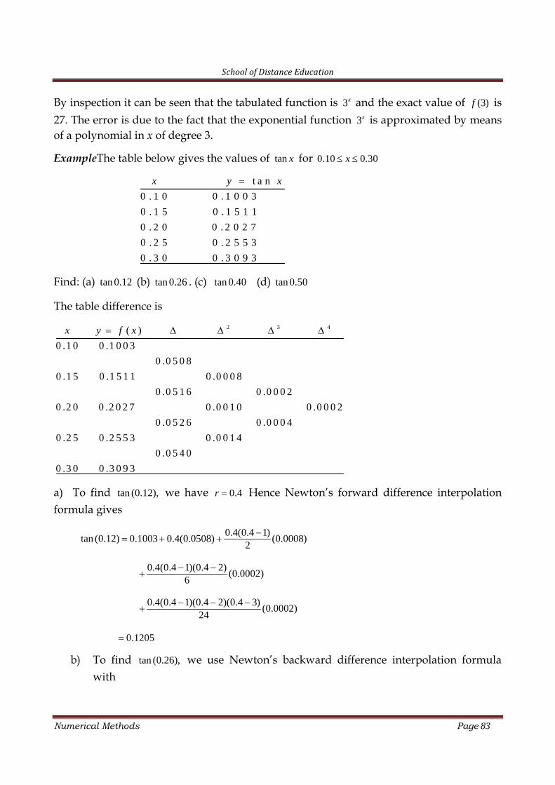
School of Distance Education
Numerical Methods Page 83
By inspection it can be seen that the tabulated function is 3x and the exact value of (3)f is27. The error is due to the fact that the exponential function 3x is approximated by meansof a polynomial in x of degree 3.
ExampleThe table below gives the values of tan x for 0.10 0.30x
t a n
0 . 1 0 0 . 1 0 0 3
0 . 1 5 0 . 1 5 1 1
0 . 2 0 0 . 2 0 2 7
0 . 2 5 0 . 2 5 5 3
0 . 3 0 0 . 3 0 9 3
x y x
Find: (a) tan 0.12 (b) tan 0.26 . (c) tan 0.40 (d) tan 0.50
The table difference is
2 3 4( )
0 .1 0 0 .1 0 0 3
0 .0 5 0 8
0 .1 5 0 .1 5 1 1 0 .0 0 0 8
0 .0 5 1 6 0 .0 0 0 2
0 .2 0 0 .2 0 2 7 0 .0 0 1 0 0 .0 0 0 2
0 .0 5 2 6 0 .0 0 0 4
0 .2 5 0 .2 5 5 3 0 .0 0 1 4
0 .0 5 4 0
0 .3 0 0 .3 0 9 3
x y f x
a) To find tan (0.12), we have 0.4r Hence Newton’s forward difference interpolationformula gives
0.4(0.4 1)tan (0.12) 0.1003 0.4(0.0508) (0.0008)
2
0.4(0.4 1)(0.4 2)(0.0002)
6
0.4(0.4 1)(0.4 2)(0.4 3)(0.0002)
24
0.1205
b) To find tan (0.26), we use Newton’s backward difference interpolation formulawith
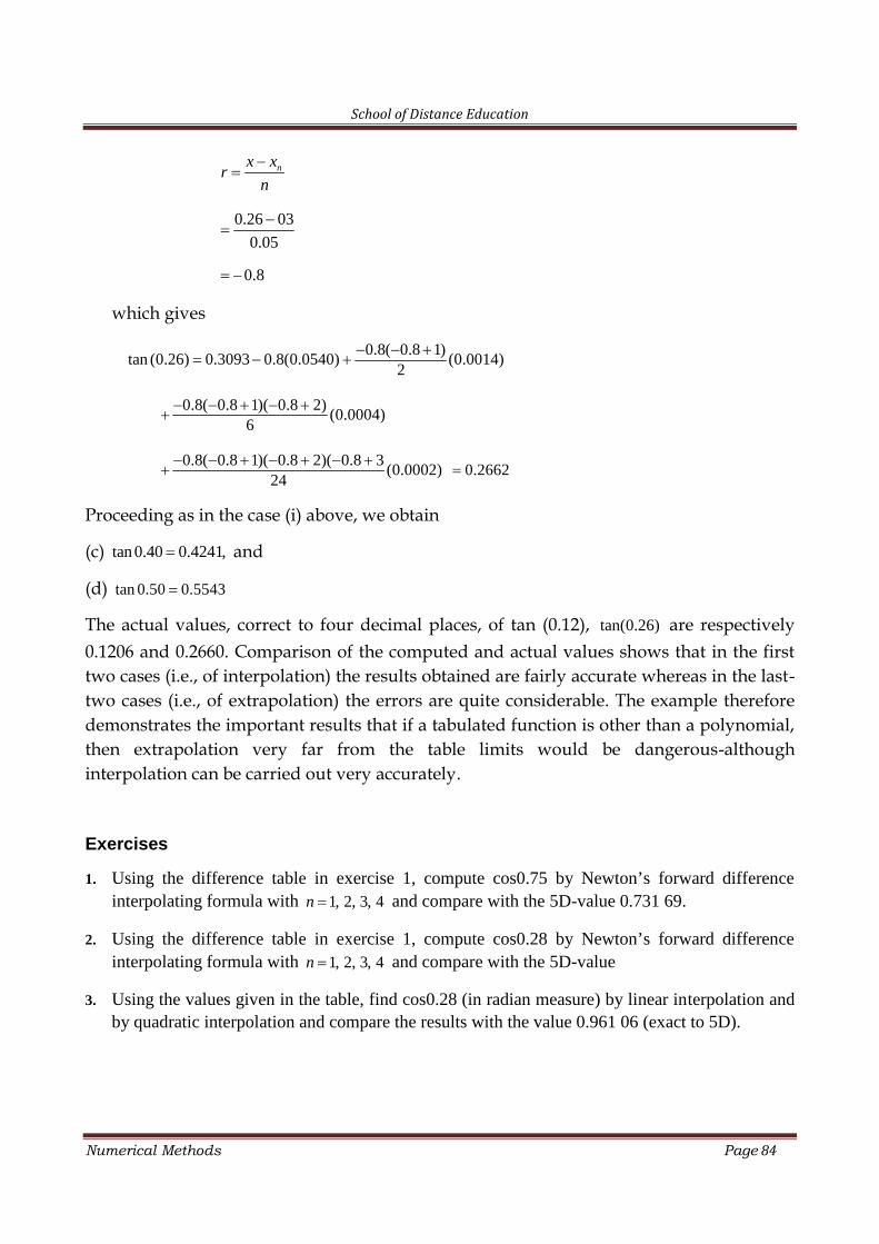
School of Distance Education
Numerical Methods Page 84
nx xr
n
0.26 03
0.05
0.8
which gives
0.8( 0.8 1)tan (0.26) 0.3093 0.8(0.0540) (0.0014)
2
0.8( 0.8 1)( 0.8 2)(0.0004)
6
0.8( 0.8 1)( 0.8 2)( 0.8 3(0.0002)
24 0.2662
Proceeding as in the case (i) above, we obtain
(c) tan 0.40 0.4241, and
(d) tan 0.50 0.5543
The actual values, correct to four decimal places, of tan (0.12), tan(0.26) are respectively0.1206 and 0.2660. Comparison of the computed and actual values shows that in the firsttwo cases (i.e., of interpolation) the results obtained are fairly accurate whereas in the last-two cases (i.e., of extrapolation) the errors are quite considerable. The example thereforedemonstrates the important results that if a tabulated function is other than a polynomial,then extrapolation very far from the table limits would be dangerous-althoughinterpolation can be carried out very accurately.
Exercises
1. Using the difference table in exercise 1, compute cos0.75 by Newton’s forward differenceinterpolating formula with 1, 2, 3, 4n and compare with the 5D-value 0.731 69.
2. Using the difference table in exercise 1, compute cos0.28 by Newton’s forward differenceinterpolating formula with 1, 2, 3, 4n and compare with the 5D-value
3. Using the values given in the table, find cos0.28 (in radian measure) by linear interpolation andby quadratic interpolation and compare the results with the value 0.961 06 (exact to 5D).
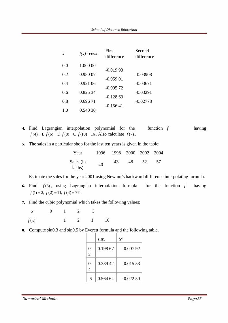
School of Distance Education
Numerical Methods Page 85
x f(x)=cosxFirstdifference
Seconddifference
0.0 1.000 00-0.019 93
-0.059 01
-0.095 72
-0.128 63
-0.156 41
-0.03908
-0.03671
-0.03291
-0.02778
0.2 0.980 07
0.4 0.921 06
0.6 0.825 34
0.8 0.696 71
1.0 0.540 30
4. Find Lagrangian interpolation polynomial for the function f having(4) 1, (6) 3, (8) 8, (10) 16f f f f . Also calculate (7)f .
5. The sales in a particular shop for the last ten years is given in the table:
Year 1996 1998 2000 2002 2004
Sales (inlakhs)
4043 48 52 57
Estimate the sales for the year 2001 using Newton’s backward difference interpolating formula.
6. Find (3)f , using Lagrangian interpolation formula for the function f having
(1) 2, (2) 11, (4) 77f f f .
7. Find the cubic polynomial which takes the following values:
x 0 1 2 3
( )f x 1 2 1 10
8. Compute sin0.3 and sin0.5 by Everett formula and the following table.
sinx 2
0.2
0.198 67 -0.007 92
0.4
0.389 42 -0.015 53
.6 0.564 64 -0.022 50
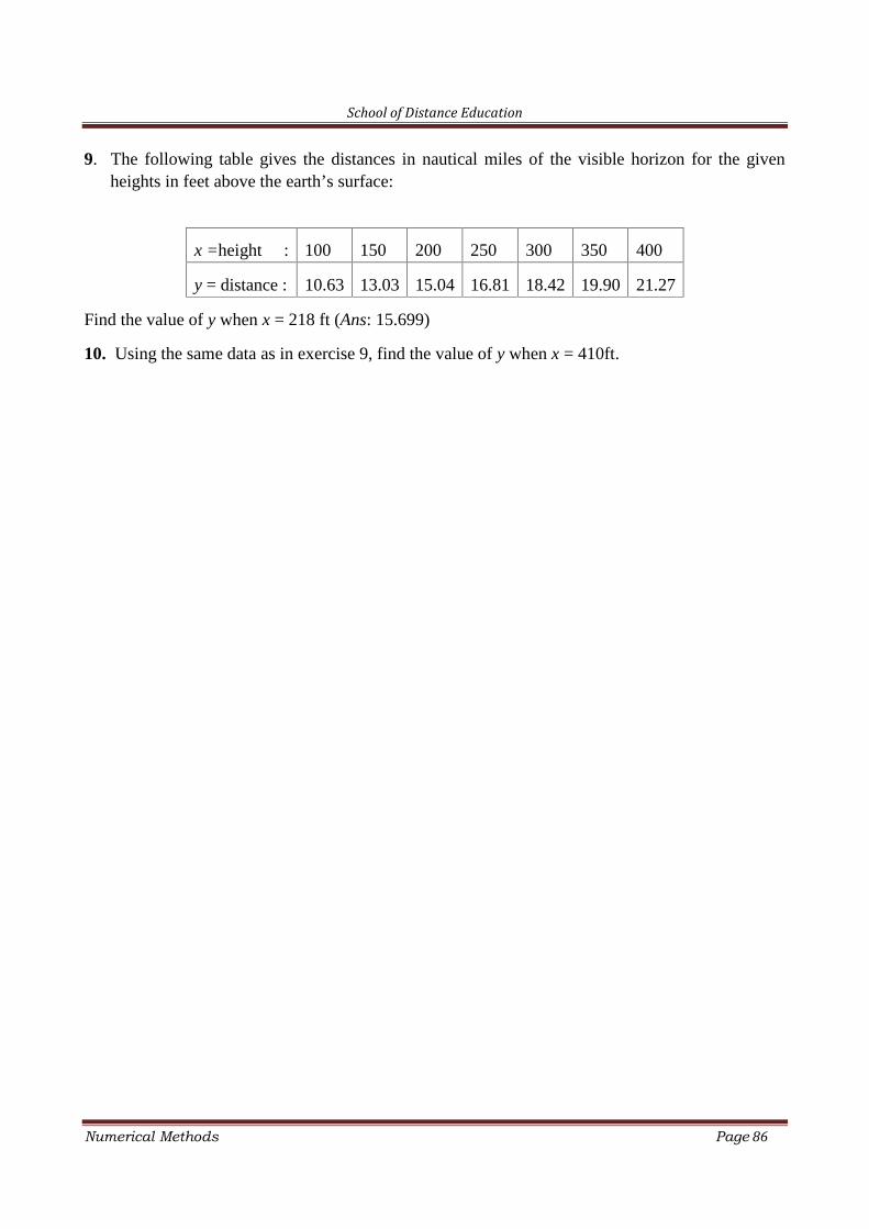
School of Distance Education
Numerical Methods Page 86
9. The following table gives the distances in nautical miles of the visible horizon for the givenheights in feet above the earth’s surface:
x =height : 100 150 200 250 300 350 400
y = distance : 10.63 13.03 15.04 16.81 18.42 19.90 21.27
Find the value of y when x = 218 ft (Ans: 15.699)
10. Using the same data as in exercise 9, find the value of y when x = 410ft.
School of Distance Education
Numerical Methods Page 87
6
NEWTON’ S AND LAGRANGIAN FORMULAE - PART I
Newton’s Backward Difference Interpolation Formula
Newton’s backward difference interpolation formula is
2 ( 1). . .( 1)( 1)( ) ( ) . . .
2! !n
n n n n n
r r r nr rf x P x f r f f f
n
where , , 0n
n
x xx x rh r n r
h
.
Derivation of Newton’s Backward Formulae for Interpolation
Given the set of ( 1)n values, viz., 0 0 1 1 2 2( , ), ( , ), ( , ),..., ( , )n nx f x f x f x f
of x and f, it is required to find ( )np x , a polynomial of the nth degree such that ( )f x and( )np x agree at the tabulated points. Let the values of x be equidistant, i.e., let
0 , 0,1,2,...,ix x rh r n
Since ( )np x is a polynomial of the nth degree, it may be written as
0 1 2 1
3 1 2
1 1
( ) ( ) ( )( )
( )( )( ) ...
( )( )...( )
n n n n
n n n
n n n
p x a a x x a x x x x
a x x x x x x
a x x x x x x
Imposing the condition that ( )f x and ( )np x should agree at the set of tabulated pointswe obtain (after some simplification) the above formula.
Remark 1:
If the values of the kth forward/backward differences are same, then (k+1)th or higher differencesare zero. Hence the given data represents a kth degree polynomial.
Remark 2:
The Backward difference Interpolation Formula is commonly used for interpolation near the end ofa set of tabular values and for extrapolating values of y a short distance forward that is right from ny
.
Problem: For the following table of values, estimate f(7.5), using Newton’s backward differenceinterpolation formula.
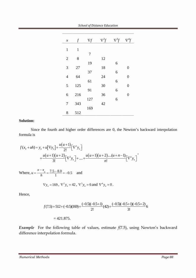
School of Distance Education
Numerical Methods Page 88
x f f 2f 3f 4f
1 17
19
37
61
91
127
169
2 8 12
18
24
30
36
42
6
6
6
6
6
3 27 0
4 64 0
5 125 0
6 216 0
7 343
8 512
Solution:
Since the fourth and higher order differences are 0, the Newton’s backward interpolationformula is
2
3
1( )
2!1 2 1 2 ....( 1)
....3! !
n n n n
nn n
u uf x uh y u y y
u u u u u u u ny y
n
,
Where, 7.5 8.0 0.51
nx x
uh
and
169ny , 2 42ny , 3 6ny and 4 0ny .
Hence,
( 0.5)( 0.5 1) ( 0.5)( 0.5 1)( 0.5 2)(7.5) 512 ( 0.5)(169) (42) 6
2! 3!f
= 421.875.
Example For the following table of values, estimate f(7.5), using Newton’s backwarddifference interpolation formula.
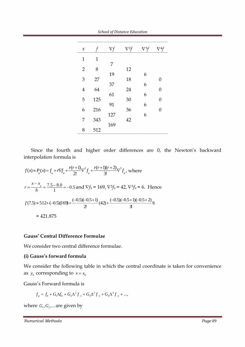
School of Distance Education
Numerical Methods Page 89
x f f 2f 3f 4f
1 17
19
37
61
91
127
169
2 8 12
18
24
30
36
42
6
6
6
6
6
3 27 0
4 64 0
5 125 0
6 216 0
7 343
8 512
Since the fourth and higher order differences are 0, the Newton’s backwardinterpolation formula is
2 3( 1) ( 1)( 2)( ) ( )
2! 3!n n n n n
r r r r rf x P x f r f f f
, where
7.5 8.0 0.51
nx x
rh
and fn = 169, 2fn = 42, 3fn = 6. Hence
6!3
)25.0)(15.0)(5.0()42(
!2
)15.0)(5.0()169)(5.0(512)5.7(
f
= 421.875
Gauss’ Central Difference Formulae
We consider two central difference formulae.
(i) Gauss’s forward formula
We consider the following table in which the central coordinate is taken for convenienceas 0y corresponding to 0x x
Gauss’s Forward formula is2 3 4
0 1 0 2 1 3 1 4 2 ...,pf f G f G f G f G f
where 1 2, ,...G G are given by
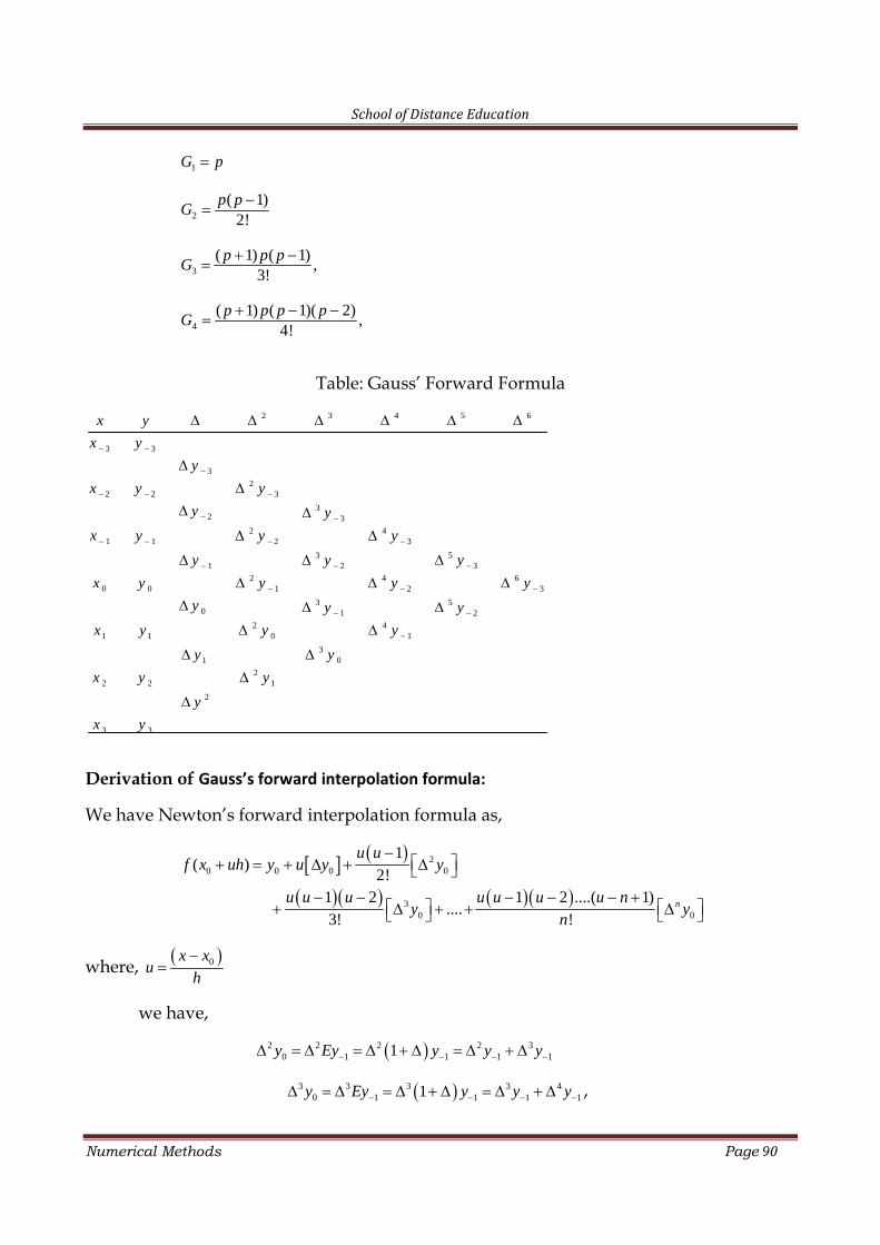
School of Distance Education
Numerical Methods Page 90
1G p
2
( 1)2!
p pG
3
( 1) ( 1),
3!p p p
G
4
( 1) ( 1)( 2),
4!p p p p
G
Table: Gauss’ Forward Formula2 3 4 5 6
3 3
3
22 2 3
32 3
2 41 1 2 3
5331 2
2 4 60 0 1 2 3
3 50 1 2
2 41 1 0 1
301
22 2 1
2
3 3
x y
x y
y
x y y
y y
x y y y
yy y
x y y y y
y y y
x y y y
yy
x y y
y
x y
Derivation of Gauss’s forward interpolation formula:
We have Newton’s forward interpolation formula as,
20 0 0 0
30 0
1( )
2!1 2 1 2 ....( 1)
....3! !
n
u uf x uh y u y y
u u u u u u u ny y
n
where, 0x xu
h
we have,
2 2 2 2 30 1 1 1 11y Ey y y y
3 3 3 3 40 1 1 1 11y Ey y y y ,
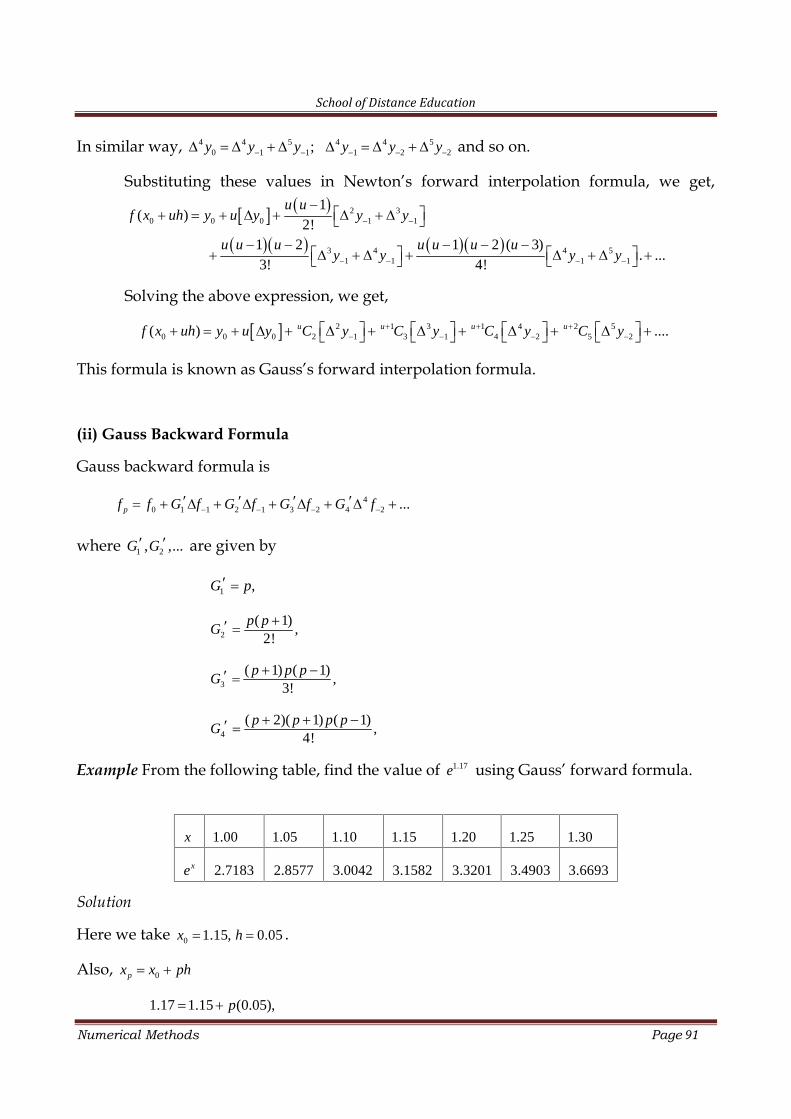
School of Distance Education
Numerical Methods Page 91
In similar way, 4 4 5 4 4 50 1 1 1 2 2;y y y y y y and so on.
Substituting these values in Newton’s forward interpolation formula, we get,
2 30 0 0 1 1
3 4 4 51 1 1 1
1( )
2!1 2 1 2 ( 3)
. ...3! 4!
u uf x uh y u y y y
u u u u u u uy y y y
Solving the above expression, we get,
2 1 3 1 4 2 50 0 0 2 1 3 1 4 2 5 2( ) ....u u u uf x uh y u y C y C y C y C y
This formula is known as Gauss’s forward interpolation formula.
(ii) Gauss Backward Formula
Gauss backward formula is
40 1 1 2 1 3 2 4 2 ...pf f G f G f G f G f
where 1 2, ,...G G are given by
1 ,G p
2
( 1),
2!p p
G
3
( 1) ( 1),
3!p p p
G
4
( 2)( 1) ( 1),
4!p p p p
G
Example From the following table, find the value of 1.17e using Gauss’ forward formula.
x 1.00 1.05 1.10 1.15 1.20 1.25 1.30
xe 2.7183 2.8577 3.0042 3.1582 3.3201 3.4903 3.6693
Solution
Here we take 0 1.15, 0.05x h .
Also, 0px x ph
1.17 1.15 (0.05),p
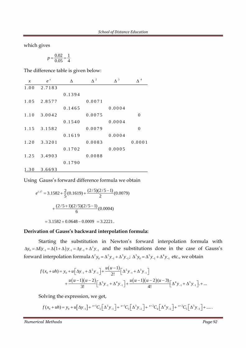
School of Distance Education
Numerical Methods Page 92
which gives
0.02 10.05 4
p
The difference table is given below:2 3 4
1 .0 0 2 .7 1 8 3
0 .1 3 9 4
1 .0 5 2 .8 5 7 7 0 .0 0 7 1
0 .1 4 6 5 0 .0 0 0 4
1 .1 0 3 .0 0 4 2 0 .0 0 7 5 0
0 .1 5 4 0 0 .0 0 0 4
1 .1 5 3 .1 5 8 2 0 .0 0 7 9 0
0 .1 6 1 9 0 .0 0 0 4
1 .2 0 3 .3 2 0 1 0 .0 0 8 3 0 .0 0 0 1
0 .1 7 0 2 0 .0 0 0 5
1 .2 5 3 .4 9 0 3 0 .0 0 8 8
0 .1 7 9 0
1 .3 0 3 .6 6 9 3
xx e
Using Gauss’s forward difference formula we obtain
1.17 (2 / 5)(2 / 5 1)23.1582 (0.1619) (0.0079)5 2
e
(2 / 5 1)(2 / 5)(2 / 5 1)(0.0004)
6
3.1582 0.0648 0.0009 3.2221 .
Derivation of Gauss’s backward interpolation formula:
Starting the substitution in Newton’s forward interpolation formula with 2
0 1 1 1 11y Ey y y y and the substitutions done in the case of Gauss’sforward interpolation formula 2 2 3
0 1 1y y y ; 3 3 40 1 1y y y etc., we obtain
2 2 30 0 1 1 1 1
3 4 4 51 1 1 1
1( )
2!1 2 1 2 ( 3)
. ...3! 4!
u uf x uh y u y y y y
u u u u u u uy y y y
Solving the expression, we get,
1 2 1 3 2 4 2 50 0 1 2 1 3 2 4 2 5 3( ) ....u u u uf x uh y u y C y C y C y C y
.
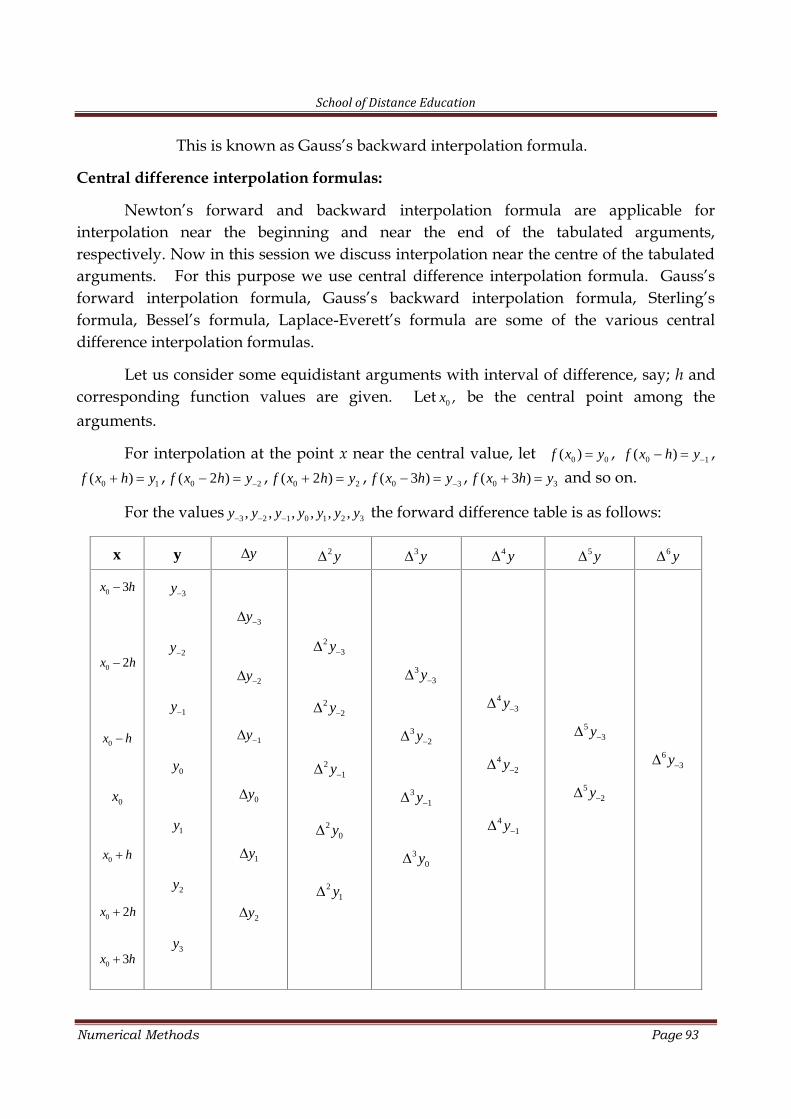
School of Distance Education
Numerical Methods Page 93
This is known as Gauss’s backward interpolation formula.
Central difference interpolation formulas:
Newton’s forward and backward interpolation formula are applicable forinterpolation near the beginning and near the end of the tabulated arguments,respectively. Now in this session we discuss interpolation near the centre of the tabulatedarguments. For this purpose we use central difference interpolation formula. Gauss’sforward interpolation formula, Gauss’s backward interpolation formula, Sterling’sformula, Bessel’s formula, Laplace-Everett’s formula are some of the various centraldifference interpolation formulas.
Let us consider some equidistant arguments with interval of difference, say; h andcorresponding function values are given. Let 0x , be the central point among thearguments.
For interpolation at the point x near the central value, let 0 0( )f x y , 0 1( )f x h y ,
0 1( )f x h y , 0 2( 2 )f x h y , 0 2( 2 )f x h y , 0 3( 3 )f x h y , 0 3( 3 )f x h y and so on.
For the values 3 2 1 0 1 2 3, , , , , ,y y y y y y y the forward difference table is as follows:
x y y 2 y 3 y 4 y 5 y 6 y
0 3x h
0 2x h
0x h
0x
0x h
0 2x h
0 3x h
3y
2y
1y
0y
1y
2y
3y
3y
2y
1y
0y
1y
2y
23y
22y
21y
20y
21y
33y
32y
31y
30y
43y
42y
41y
53y
52y
63y
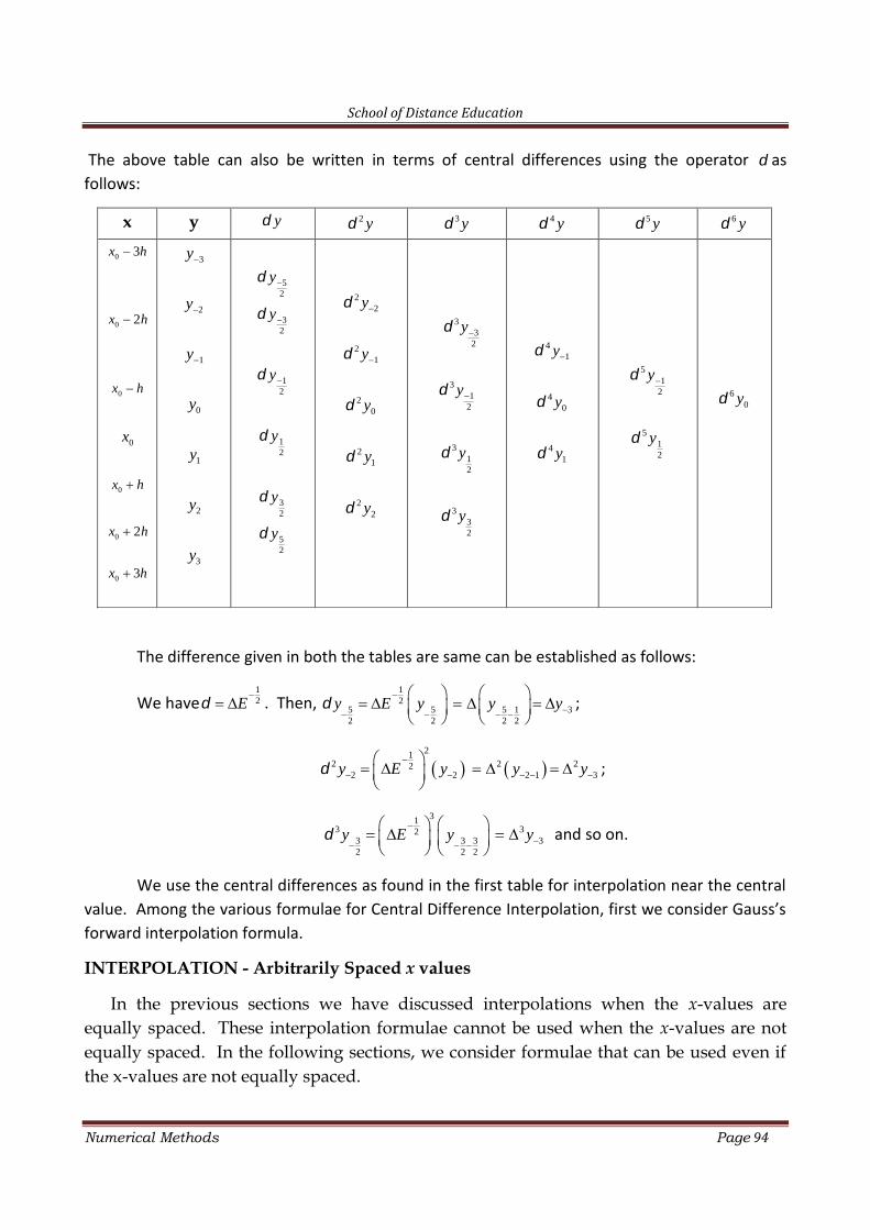
School of Distance Education
Numerical Methods Page 94
The above table can also be written in terms of central differences using the operator asfollows:
x y y 2 y 3 y 4 y 5 y 6 y
0 3x h
0 2x h
0x h
0x
0x h
0 2x h
0 3x h
3y
2y
1y
0y
1y
2y
3y
52
y
32
y
12
y
12
y
32
y
52
y
22y
21y
20y
21y
22y
33
2
y
31
2
y
312
y
332
y
41y
40y
41y
51
2
y
512
y
60y
The difference given in both the tables are same can be established as follows:
We have12E
. Then,12
5 5 5 1 32 2 2 2
y E y y y
;
21
2 2 222 2 2 1 3y E y y y
;
313 32
3 3 3 32 2 2
y E y y
and so on.
We use the central differences as found in the first table for interpolation near the centralvalue. Among the various formulae for Central Difference Interpolation, first we consider Gauss’sforward interpolation formula.
INTERPOLATION - Arbitrarily Spaced x values
In the previous sections we have discussed interpolations when the x-values areequally spaced. These interpolation formulae cannot be used when the x-values are notequally spaced. In the following sections, we consider formulae that can be used even ifthe x-values are not equally spaced.
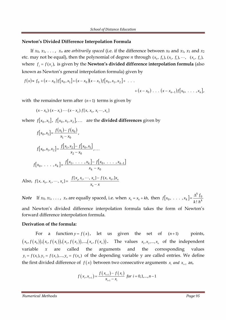
School of Distance Education
Numerical Methods Page 95
Newton’s Divided Difference Interpolation Formula
If x0, x1, . . . , xn are arbitrarily spaced (i.e. if the difference between x0 and x1, x1 and x2
etc. may not be equal), then the polynomial of degree n through 0 0 1 1( , ), ( , ), ,x f x f ( , ),n nx f
where ( ),j jf f x is given by the Newton’s divided difference interpolation formula (alsoknown as Newton’s general interpolation formula) given by
...,,, 210101000 xxxfxxxxxxfxxfxf
nn xxfxxxx ,...,... 010 ,
with the remainder term after ( 1)n terms is given by
0 1 0 1( ) ( ) ( ) [ , , , ]n nx x x x x x f x x x x
where 10 , xxf , 210 ,, xxxf , are the divided differences given by
01
0110 ,
xx
xfxfxxf
,
02
1021210
,,,,
xx
xxfxxfxxxf
,
0
1010
,...,,...,,...,
xx
xxfxxfxxf
k
kkk
Also, 0 1[ , , , , ]nf x x x x 1 0
0
[ , , ] ( , , ]p n nf x x x f x x x
x x
Note If x0, x1, . . . , xn are equally spaced, i.e. when 0 ,kx x kh then k
k
khk
fxxf
!,..., 0
0
and Newton’s divided difference interpolation formula takes the form of Newton’sforward difference interpolation formula.
Derivation of the formula:
For a function y f x , let us given the set of ( 1)n points,
0 0 1 1 2 2, , , , , ,..., ,n nx f x x f x x f x x f x . The values 1 2, ,..., nx x x of the independentvariable x are called the arguments and the corresponding values
1 1 2 2( ), ( ),..., ( )n ny f x y f x y f x of the depending variable y are called entries. We definethe first divided difference of f x between two consecutive arguments 1i ix and x as,
11
1
, 0,1,..., 1i ii i
i i
f x f xf x x for i n
x x
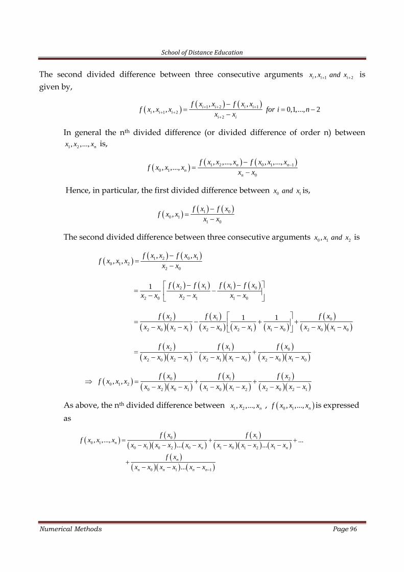
School of Distance Education
Numerical Methods Page 96
The second divided difference between three consecutive arguments 1 2,i i ix x and x isgiven by,
1 2 11 2
2
, ,, , 0,1,..., 2i i i i
i i ii i
f x x f x xf x x x for i n
x x
In general the nth divided difference (or divided difference of order n) between1 2, ,..., nx x x is,
1 2 0 1 10 1
0
, ,..., , ,...,, ,..., n n
nn
f x x x f x x xf x x x
x x
Hence, in particular, the first divided difference between 0 1x and x is,
1 00 1
1 0
,f x f x
f x xx x
The second divided difference between three consecutive arguments 0 1 2,x x and x is
1 2 0 10 1 2
2 0
, ,, ,
f x x f x xf x x x
x x
2 1 1 0
2 0 2 1 1 0
1 f x f x f x f xx x x x x x
2 1 0
2 0 2 1 2 0 2 1 1 0 2 0 1 0
1 1f x f x f x
x x x x x x x x x x x x x x
2 1 0
2 0 2 1 2 1 1 0 2 0 1 0
f x f x f x
x x x x x x x x x x x x
0 1 20 1 2
0 2 0 1 1 0 1 2 2 0 2 1
, ,f x f x f x
f x x xx x x x x x x x x x x x
As above, the nth divided difference between 1 2, ,..., nx x x , 0 1, ,..., nf x x x is expressedas
0 10 1
0 1 0 2 0 1 0 1 2 1
0 1 1
, ,..., ...... ...
...
nn n
n
n n n n
f x f xf x x x
x x x x x x x x x x x x
f x
x x x x x x
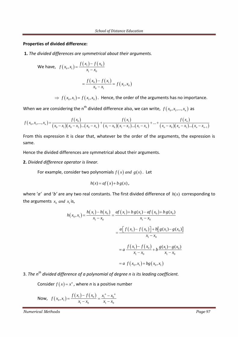
School of Distance Education
Numerical Methods Page 97
Properties of divided difference:
1. The divided differences are symmetrical about their arguments.
We have, 1 00 1
1 0
,f x f x
f x xx x
0 11 0
0 1
,f x f x
f x xx x
0 1 1 0, ,f x x f x x . Hence, the order of the arguments has no importance.
When we are considering the nth divided difference also, we can write, 0 1, ,..., nf x x x as
0 10 1
0 1 0 2 0 1 0 1 2 1 0 1 1
, ,..., ...... ... ...
nn
n n n n n n
f x f x f xf x x x
x x x x x x x x x x x x x x x x x x
From this expression it is clear that, whatever be the order of the arguments, the expression issame.
Hence the divided differences are symmetrical about their arguments.
2. Divided difference operator is linear.
For example, consider two polynomials ( )f x and g x . Let
( ) ( )h x af x b g x ,
where ‘a’ and ‘b’ are any two real constants. The first divided difference of ( )h x corresponding tothe arguments 0 1x and x is,
1 0 1 1 0 00 1
1 0 1 0
( ) ( ),
h x h x af x b g x af x b g xh x x
x x x x
1 0 1 0
1 0
( ) ( )a f x f x b g x g x
x x
1 0 1 0
1 0 1 0
( ) ( )f x f x g x g xa b
x x x x
0 1 0 1, ,a f x x bg x x
3. The nth divided difference of a polynomial of degree n is its leading coefficient.
Consider nf x x , where n is a positive number
Now, 1 0 1 00 1
1 0 1 0
,n nf x f x x x
f x xx x x x
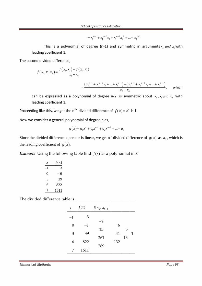
School of Distance Education
Numerical Methods Page 98
1 2 3 2 11 1 0 1 0 0...n n n nx x x x x x
This is a polynomial of degree (n-1) and symmetric in arguments 1ox and x withleading coefficient 1.
The second divided difference,
1 2 0 10 1 2
2 0
, ,, ,
f x x f x xf x x x
x x
1 2 1 1 2 12 2 1 1 0 0 1 1
2 0
... ...n n n n n nx x x x x x x x
x x
, which
can be expressed as a polynomial of degree n-2, is symmetric about 0 1 2,x x and x withleading coefficient 1.
Proceeding like this, we get the nth divided difference of nf x x is 1.
Now we consider a general polynomial of degree n as,
1 20 1 2 ...n n n
ng x a x a x a x a
Since the divided difference operator is linear, we get nth divided difference of g x as 0a , which is
the leading coefficient of g x .
Example Using the following table find ( )f x as a polynomial in x
( )
1 3
0 6
3 39
6 822
7 1611
x f x
The divided difference table is
x ( )f x 1[ , ]k kf x x
1
0
3
6
7
3
6
39
822
1611
9
15
261
789
6
41
132
5
131
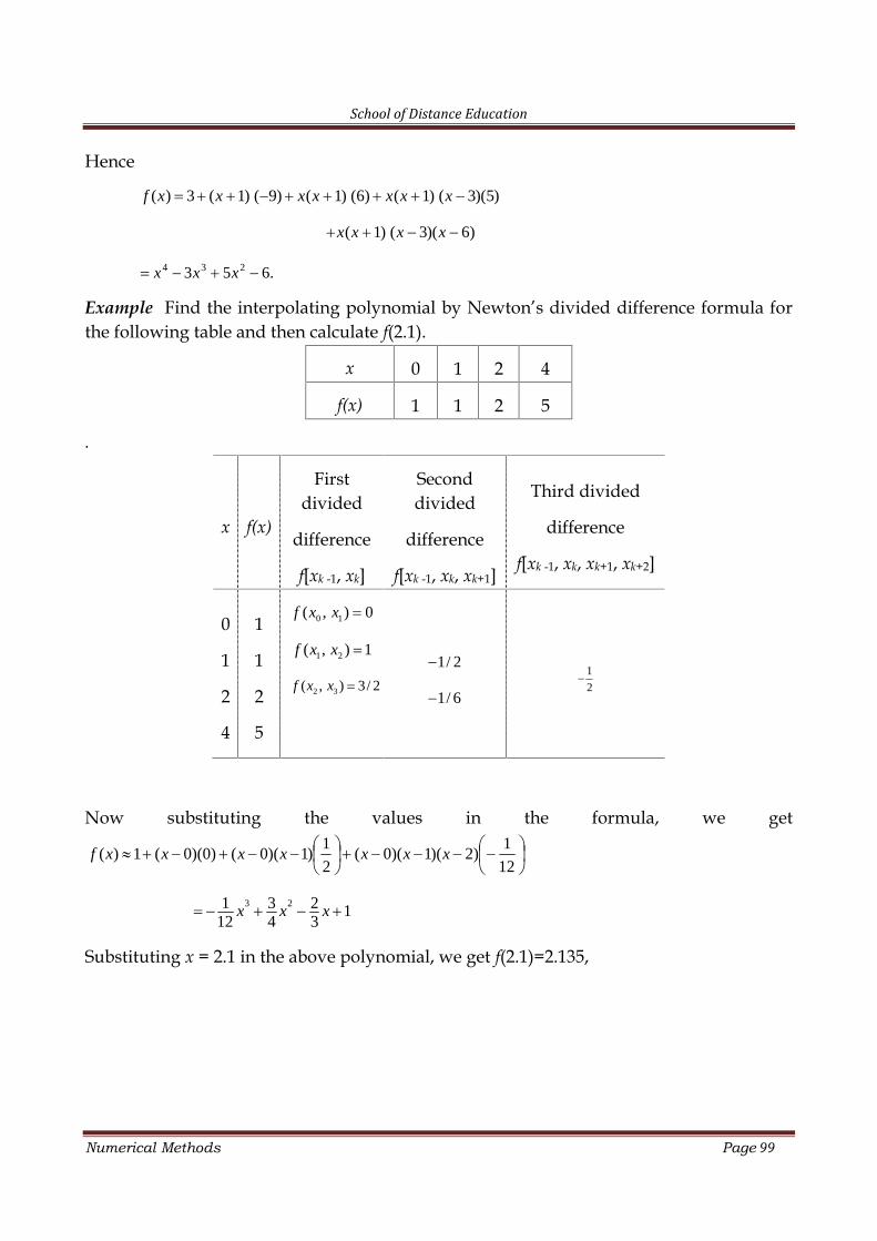
School of Distance Education
Numerical Methods Page 99
Hence
( ) 3 ( 1) ( 9) ( 1) (6) ( 1) ( 3)(5)f x x x x x x x
( 1) ( 3)( 6)x x x x
4 3 23 5 6.x x x
Example Find the interpolating polynomial by Newton’s divided difference formula forthe following table and then calculate f(2.1).
x 0 1 2 4
f(x) 1 1 2 5
.
x f(x)
Firstdivided
difference
f[xk -1, xk]
Seconddivided
difference
f[xk -1, xk, xk+1]
Third divided
difference
f[xk -1, xk, xk+1, xk+2]
0
1
2
4
1
1
2
5
0 1( , ) 0f x x
1 2( , ) 1f x x
2 3( , ) 3/ 2f x x
1/ 2
1/ 6
1
2
Now substituting the values in the formula, we get
12
1)2)(1)(0(
2
1)1)(0()0)(0(1)( xxxxxxxf
3 21 3 2 112 4 3
x x x
Substituting x = 2.1 in the above polynomial, we get f(2.1)=2.135,
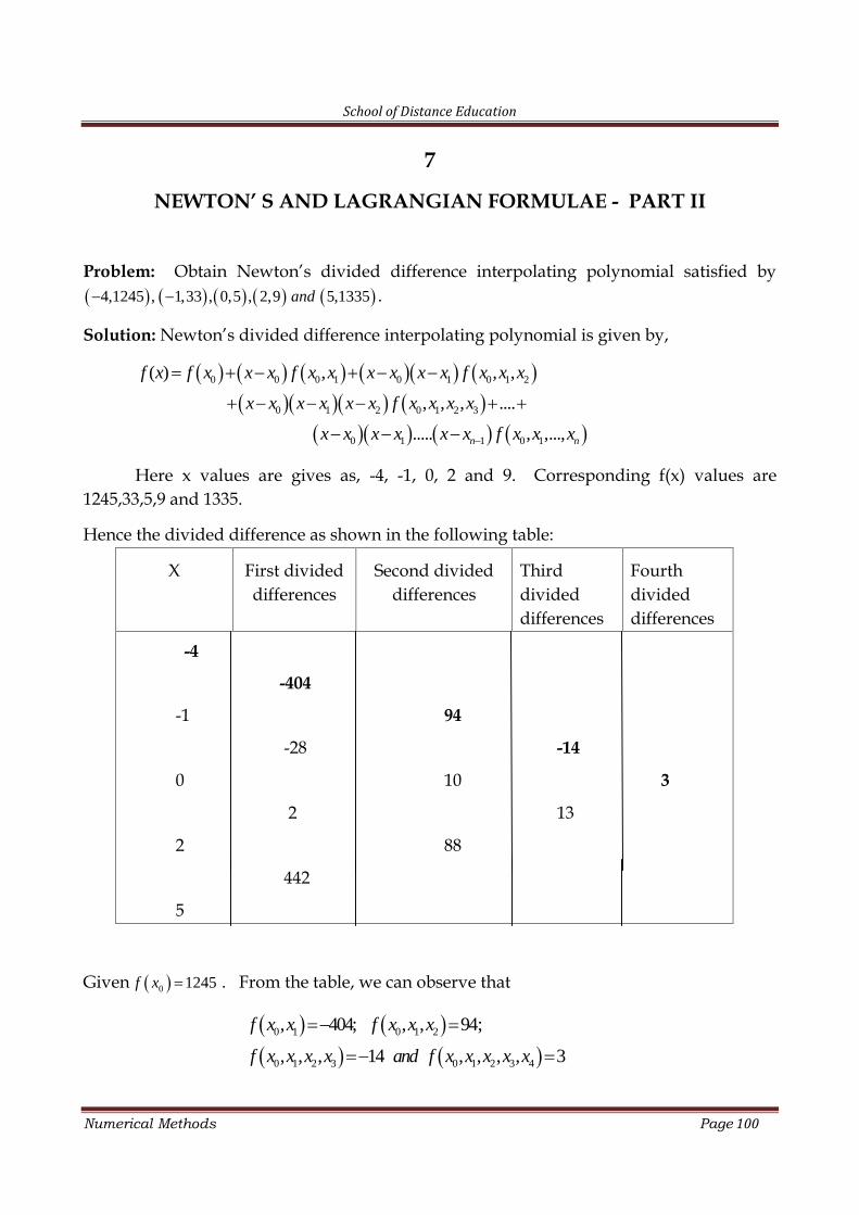
School of Distance Education
Numerical Methods Page 100
7
NEWTON’ S AND LAGRANGIAN FORMULAE - PART II
Problem: Obtain Newton’s divided difference interpolating polynomial satisfied by 4,1245 , 1,33 , 0,5 , 2,9 5,1335and .
Solution: Newton’s divided difference interpolating polynomial is given by,
0 0 0 1 0 1 0 1 2
0 1 2 0 1 2 3
0 1 1 0 1
( ) , , ,
, , , ....
..... , ,...,n n
f x f x x x f x x x x x x f x x x
x x x x x x f x x x x
x x x x x x f x x x
Here x values are gives as, -4, -1, 0, 2 and 9. Corresponding f(x) values are1245,33,5,9 and 1335.
Hence the divided difference as shown in the following table:
X First divideddifferences
Second divideddifferences
Thirddivideddifferences
Fourthdivideddifferences
-4
-404
-1 94
-28 -14
0 10 3
2 13
2 88
442
5
Given 0 1245f x . From the table, we can observe that
0 1 0 1 2
0 1 2 3 0 1 2 3 4
, 404; , , 94;
, , , 14 , , , , 3
f x x f x x x
f x x x x and f x x x x x
School of Distance Education
Numerical Methods Page 101
Hence the interpolating polynomial is,
( ) 1245 ( 4) ( 404) ( 4) ( 1) 94
( 4) ( 1) 0 14 ( 4) ( 1) 0 2 3
f x x x x
x x x x x x x
( ) 1245 404 4 94 4 1
14 4 1 0 3 4 1 0 2
f x x x x
x x x x x x x
On simplification, we get,
4 3 2( ) 3 5 6 14 5f x x x x x .
Newton’s Interpolation formula with divided differences
Consider two arguments 0x and x . The first divided difference between 0x and x is,
0 00
0 0
,f x f x f x f x
f x xx x x x
0 0 0,f x f x x x f x x ---- (1)
Consider 0 1,x x and x . Then,
0 1 0 0 0 10 1
1 1
, , , ,, ,
f x x f x x f x x f x xf x x x
x x x x
0 0 1 1 0 1, , , ,f x x f x x x x f x x x
Put it in (1), we get,
0 0 0 1 1 0 1, , ,f x f x x x f x x x x f x x x
That is,
0 0 0 1 0 1 0 1, , ,f x f x x x f x x x x x x f x x x --- (2)
Again, for 0 1 2, ,x x x and x
0 1 0 1 2 0 1 2 0 10 1 2
2 2
, , , , , , , ,, , ,
f x x x f x x x f x x x f x x xf x x x x
x x x x
0 1 2 0 1 2 0 1 2, , , , , , ,f x x x x x f x x x x f x x x
School of Distance Education
Numerical Methods Page 102
Hence (2) implies,
0 0 0 1 0 1 2 0 1 2 0 1 2, , , , , ,f x f x x x f x x x x x x x x f x x x x f x x x
0 0 0 1 0 1 0 1 2 0 1 2 0 1 2, , , , , ,f x x x f x x x x x x f x x x x x x x x x f x x x x
Proceeding like this, we obtain for f x as,
0 0 0 1 0 1 0 1 2
0 1 2 0 1 2 3
0 1 0 1
( ) , , ,
, , , ....
..... , , ,...,n n
f x f x x x f x x x x x x f x x x
x x x x x x f x x x x
x x x x x x f x x x x
If f(x) is a polynomial of degree n, then 0 1, , ,..., 0nf x x x x , because it is the (n+1)thdifference.
Hence we get,
0 0 0 1 0 1 0 1 2
0 1 2 0 1 2 3
0 1 1 0 1
( ) , , ,
, , , ....
..... , ,...,n n
f x f x x x f x x x x x x f x x x
x x x x x x f x x x x
x x x x x x f x x x
This is known as Newton’s interpolation formula with divided difference.
Note:
1. For the given arguments 1 2, ,..., nx x x , if all the kth , (k<n) divided differences are equal,the k+1th divided differences are zeroes. Then Newton’s interpolation formula gives apolynomial of degree k for the given data.
2. Newton’s divided difference interpolation formula possesses the permanence property.Apart from the given arguments 1 2, ,..., nx x x along with the corresponding function values,suppose that on a later time a new argument 1nx with corresponding entry 1( )nf x aregiven. The new set of data values can be represented by a polynomial of degree (n+1). Toobtain the required polynomial we add the term 0 1 0 1 1..... , ,..., ,n n nx x x x x x f x x x x tothe previously obtained nth degree polynomial.
Problem 2: The following table gives the relation between steam pressure andtemperature. Find the pressure at temperature 3750.
Temp. : 3610 3670 3780 3870 3990
Pressure: 154.9 167.9 191 212.5 244.2
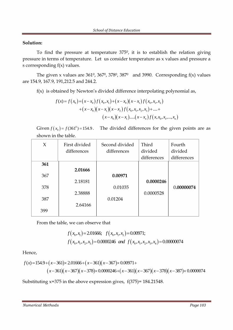
School of Distance Education
Numerical Methods Page 103
Solution:
To find the pressure at temperature 3750, it is to establish the relation givingpressure in terms of temperature. Let us consider temperature as x values and pressure as corresponding f(x) values.
The given x values are 3610, 3670, 3780, 3870 and 3990. Corresponding f(x) valuesare 154.9, 167.9, 191,212.5 and 244.2.
f(x) is obtained by Newton’s divided difference interpolating polynomial as,
0 0 0 1 0 1 0 1 2
0 1 2 0 1 2 3
0 1 0 1
( ) , , ,
, , , ....
..... , , ,...,n n
f x f x x x f x x x x x x f x x x
x x x x x x f x x x x
x x x x x x f x x x x
Given 00 (361 ) 154.9f x f . The divided differences for the given points are as
shown in the table.
X First divideddifferences
Second divideddifferences
Thirddivideddifferences
Fourthdivideddifferences
3612.01666
367 0.009712.18181 0.0000246
378 0.01035 0.000000742.38888 0.0000528
387 0.012042.64166
399
From the table, we can observe that
0 1 0 1 2
0 1 2 3 0 1 2 3 4
, 2.01666; , , 0.00971;
, , , 0.0000246 , , , , 0.00000074
f x x f x x x
f x x x x and f x x x x x
Hence,
( ) 154.9 361 2.01666 361 367 0.00971
361 367 378 0.0000246 361 367 378 387 0.0000074
f x x x x
x x x x x x x
Substituting x=375 in the above expression gives, f(375)= 184.21548.
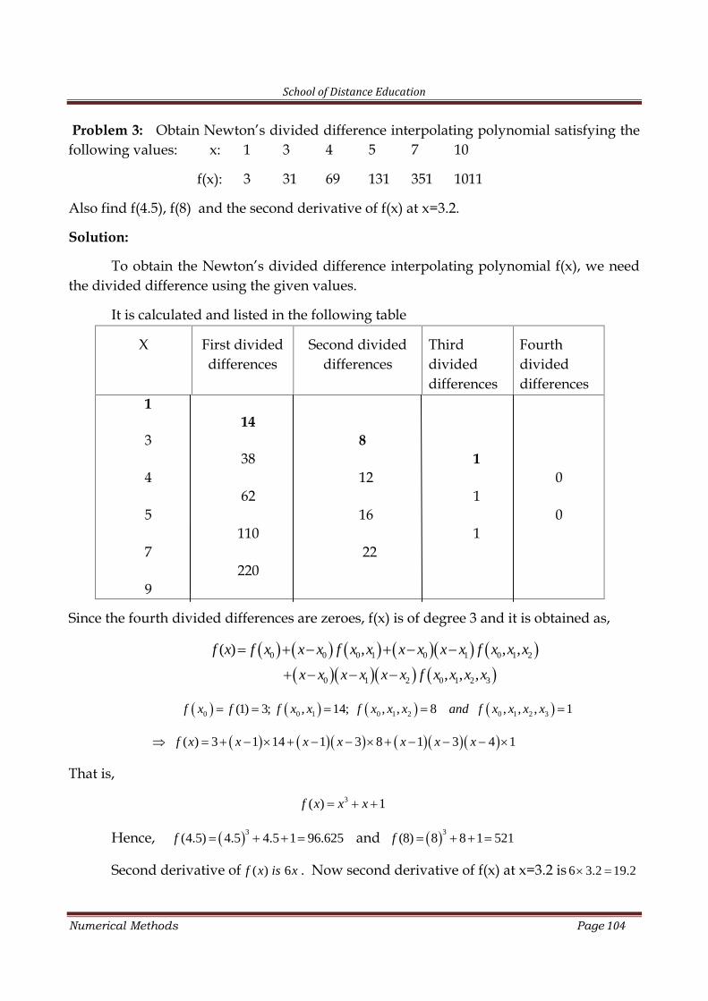
School of Distance Education
Numerical Methods Page 104
Problem 3: Obtain Newton’s divided difference interpolating polynomial satisfying thefollowing values: x: 1 3 4 5 7 10
f(x): 3 31 69 131 351 1011
Also find f(4.5), f(8) and the second derivative of f(x) at x=3.2.
Solution:
To obtain the Newton’s divided difference interpolating polynomial f(x), we needthe divided difference using the given values.
It is calculated and listed in the following table
X First divideddifferences
Second divideddifferences
Thirddivideddifferences
Fourthdivideddifferences
114
3 838 1
4 12 062 1
5 16 0110 1
7 22220
9
Since the fourth divided differences are zeroes, f(x) is of degree 3 and it is obtained as,
0 0 0 1 0 1 0 1 2
0 1 2 0 1 2 3
( ) , , ,
, , ,
f x f x x x f x x x x x x f x x x
x x x x x x f x x x x
0 0 1 0 1 2 0 1 2 3(1) 3; , 14; , , 8 , , , 1f x f f x x f x x x and f x x x x
( ) 3 1 14 1 3 8 1 3 4 1f x x x x x x x
That is,3( ) 1f x x x
Hence, 3(4.5) 4.5 4.5 1 96.625f and 3(8) 8 8 1 521f
Second derivative of ( ) 6f x is x . Now second derivative of f(x) at x=3.2 is 6 3.2 19.2
School of Distance Education
Numerical Methods Page 105
Lagrangian Interpolation
Another method of interpolation in the case of arbitrarily spaced pivotal values x0, x1, . . ., xn is Lagrangian interpolation. This method is based on Lagrange’s n+1 pointinterpolation formula given by
n
kk
kk
kn f
xl
xlxLxf
0,
where
0 1 2( ) ( )( ) . . . . ( )
nl x x x x x x x ,
0 1 1( ) ( ) ( )( ) ( )k k k nl x x x x x x x x x , 0 < k < n.
0 1 1( ) ( )( ) . . ..( )
n nl x x x x x x x
Remark: ( ) .k k k
L x f For, ( ) 0, ,k j
l x when j k so that fork
x x , the sum on the RHS of the
formula reduces to the single termk
f , which indicates that f andk
L agrees at n+1
tabulated points.
Derivation of the formula:
Given the set of ( 1)n points, 0 0 1 1 2 2, , , , , ,..., ,n nx f x x f x x f x x f x of x and f(x), it is
required to fit the unique polynomial ( )np x of maximum degree n, such that ( )f x and ( )np x agree
at the given set of points. The values 0 1, ,..., nx x x may not be equidistant.
Since the interpolating polynomial must use all the ordinates 0 1, ,..., nf x f x f x , it can be
written as a linear combination of these ordinates. That is, we can write the polynomial as
0 0 1 1( ) ( ) ( ) ( ) .n n np x l x f x l x f x l x f x
where ( ), 0,1,2,...,i if x and l x for i n are polynomials of degree n.
This polynomial fits the given data exactly.
At 0x x , as ( )np x and ( )f x coincide, we get,
0 0 0 0 0 1 0 1 0( ) ( ) ( ) ( ) ... ( )n n nf x p x l x f x l x f x l x f x
This equation is satisfied only when 0 0( ) 1l x and 0( ) 0, 0il x i
School of Distance Education
Numerical Methods Page 106
At a general point ix x , we get,
0 0 1 1( ) ( ) ( ) ( ) ... ( )i n i i i n i nf x p x l x f x l x f x l x f x
This equation is satisfied only when ( ) 1i il x and ( ) 0,j il x i j
Therefore, ( )il x , which are polynomials of degree n, satisfy the conditions
Since, ( ) 0il x at 0 1 1 1, ,..., , ,...,i i nx x x x x x , we know that
0 1 1 1, ,..., , ,...,i i nx x x x x x x x x x are factors of ( )il x . The product of these factors is a
polynomial of degree n. Therefore, we can write
0 1 1 1( ) ... ...i i i nl x C x x x x x x x x x x , where C is a constant.
Now, since ( ) 1i il x , we get
0 1 1 1( ) 1 ... ...i i i i i i i i i nl x C x x x x x x x x x x
Hence, 0 1 1 1
1... ...i i i i i i i n
Cx x x x x x x x x x
Therefore,
0 1 1 1
0 1 1 1
... ...( )
... ...i i n
ii i i i i i i n
x x x x x x x x x xl x
x x x x x x x x x x
Now the polynomial
0 0 1 1( ) ( ) ( ) ... ( )n n np x l x f x l x f x l x f x ,
with
0 1 1 1
0 1 1 1
... ...( )
... ...i i n
ii i i i i i i n
x x x x x x x x x xl x
x x x x x x x x x x
is called Lagrange interpolating
polynomial and ( )il x are called Lagrange fundamental polynomials.
To fit a polynomial of degree 1, we require at least two points. Let 0 0 1 1, , ,x f x x f x
are the points. Then the Lagrange polynomial of degree one or a straight line for the given data is,
1 0 0 1 1( ) ( ) ( )p x l x f x l x f x , where,
10
0 1
( )x x
l xx x
and
01
1 0
( )x x
l xx x
.
Let 0 0 1 1 2 2, , , , ,x f x x f x x f x are the given three points. Then the Lagrange
polynomial of degree two for the data is given by
1,( )
0,i j
i jl x
i j
School of Distance Education
Numerical Methods Page 107
2 0 0 1 1 2 2( ) ( ) ( ) ( )p x l x f x l x f x l x f x , where,
1 20
0 1 0 2
( )x x x x
l xx x x x
,
0 21
1 0 1 2
( )x x x x
l xx x x x
and
0 12
2 0 2 1
( )x x x x
l xx x x x
.
For the four points 0 0 1 1 2 2 3 3, , , , , , ,x f x x f x x f x x f x , the Lagrange polynomial of
degree three is given by,
3 0 0 1 1 2 2 3 3( ) ( ) ( ) ( ) ( )p x l x f x l x f x l x f x l x f x , where,
1 2 30
0 1 0 2 0 3
( )x x x x x x
l xx x x x x x
0 2 31
1 0 1 2 1 3
( )x x x x x x
l xx x x x x x
,
0 1 32
2 0 2 1 2 3
( )x x x x x x
l xx x x x x x
and
0 1 23
3 0 3 1 3 2
( )x x x x x x
l xx x x x x x
and so on.
Problem : Given f(2) = 9, and f(6) = 17. Find an approximate value for f(5) by the method ofLagrange’s interpolation.
Solution:
For the given two points (2,9) and (6,17), the Lagrangian polynomial of degree 1 is
1 0 0 1 1( ) ( ) ( )p x l x f x l x f x , where,
10
0 1
( )x x
l xx x
and
01
1 0
( )x x
l xx x
. That is,
1 01 0 1
0 1 1 0
( )x x x x
p x f x f xx x x x
1
6 2( ) 9 17
2 6 6 2
x xp x
Hence,
1
5 6 5 2(5) (5) 9 17
2 6 6 2
1 39 174 4
15
f P
Problem: Use Lagrange’s formula, to find the quadratic polynomial that takes the values
: 0 1 3
( ) : 0 1 0
x
f x
School of Distance Education
Numerical Methods Page 108
For the given three points (0,0) , (1,1) and (3,0), the quadratic polynomial by Lagrange’s
interpolation is
1 2 0 2 0 12 0 1 2
0 1 0 2 1 0 1 2 2 0 2 1
( )x x x x x x x x x x x x
p x f x f x f xx x x x x x x x x x x x
We are considering the given x values 0,1, and 3 as 0 1 2,x x and x . Given, 0 2( )f x and f x
are zeroes. Hence the polynomial is,
0 22 1
1 0 1 2
( )x x x x
p x f xx x x x
Then,
2
0 3( ) 1
1 0 1 3
x xp x
22
3 1( ) 1 32 2
x xp x x x
.
Example Find Lagrange’s interpolation polynomial fitting the points f(1) = 3, f(3) = 0,f(4) = 30, f(6) = 132. Hence find f(5).
Here 4 tabulated points are given. Hence we need Lagrange’s polynomial for (n + = 3+ 1 = 4 points) and is given by
3
30
( )( ) ( )
( )k
kk k k
l xf x L x f
l x
.
Now substituting the values, we obtain
)0()63)(43)(13(
)6)(4)(1()3(
)61)(41)(31(
)6)(4)(3(3
xxxxxx
xL
)132()46)(46)(16(
)4)(3)(1()30(
)64)(34)(14(
)6)(3)(1(
xxxxxx
3 21 ( 27 92 60),2
x x x on simplification.
Now 3 2
3
1(5) (5) (5) 27(5) 92(5) 60 75.2
f L
Example Find ln 9.2 with 3n , using Lagrange’s interpolation formula with the giventable:
x 9.0 9.5 10.0 11.0
ln x 2.197 2.251 2.302 2.397
School of Distance Education
Numerical Methods Page 109
22 29 59 90
3
30
(9.2)ln(9.2) (9.2) 9.2
( )k
kk k k
lf L f
l x
.
(9.2 9.5)(9.2 10.0)(9.2 11.0)(2.19722)
(9.0 9.5)(9.0 10.0)(9.0 11.0)
(9.2 9.0)(9.2 10.0)(9.2 11.0)(2.25129)
(9.5 9.0)(9.5 10.0)(9.5 11.0)
(9.2 9.0)(9.2 9.5)(9.2 11.0)(2.30259)
(10.0 9.0)(10.0 9.5)(10.0 11.0)
(9.2 9.0)(9.2 9.5)(9.2 10.0)(2.39790)
(11.0 9.0)(11.0 9.5)(11.0 10.0)
= 2.219 20, which is exact to 5D.
Example Certain corresponding values of x and 10log x are(300, 2.4771), (304, 2.4829), (305, 2.4843) and (307, 2.4871). Find 10log 301.
10( 3) ( 4) ( 6) (1) ( 4) ( 6)
log 301 (2.4771) (2.4829)( 4) ( 5) ( 7) (4) ( 1) ( 3)
(1) ( 3) ( 6) (1) ( 3) ( 4)(2.4843) (2.4871)
(5) (1) ( 2) (7) (3) (2)
1.2739 4.9658 4.4717 0.7106
2.4786.
Inverse Lagrangian Interpolation Formula
Interchanging x and y in the Lagrangian Interpolation Formula, we obtain the inverseLagrangian interpolation formula given by
0
( )( ) .
( )
nk
n kk k k
l yx L y x
l y
Example If 1 3 44, 12, 19y y y and 7,xy find x. Compare with the actual value.
Using the inverse interpolation formula,2
0
(7)(7)
( )k
n kk k k
lx L x
l y
where 0 01, ,x y k 13, 12yx y 2 24, 19x y and 7y
School of Distance Education
Numerical Methods Page 110
i.e., 0 21 20
0 1 0 2 1 0 1 2
(7 ) (7 )(7 ) (7 )
( ) ( ) ( ) ( )
y yy yx x
y y y y y y y y
0 11 2
2 0 2 1
(7 ) (7 )
( ) ( )
y yx x
y y y y
i.e.,
( 5) ( 12) (3) ( 12) (3) ( 5)(1) (3) (4)
( 8) ( 15) (8) ( 7) (15) (7)x
1 27 42 14 7
= 1.86
The actual value is 2.0 since the above values were obtained from the polynomial2( ) 3.y x x
Example Find the Lagrange interpolating polynomial of degree 2 approximating thefunction lny x defined by the following table of values. Hence determine the value of ln2.7.
ln
2 0.69315
2.5 0.91629
3.0 1.09861
x y x
Similarly,
21( ) (4 20 24)l x x x and 2
2 ( ) 2 9 10.l x x x
Hence
0 1 22 0 1 2
0 1 0
( ) ( ) ( )( )
( ) ( ) ( )k k k
l x l x l xL x f f f
l x l x l x
( 2.5) ( 3.0)( 0.5) ( 1.0)
x x0 1 2
( 2) ( 3) ( 2) ( 2.5)
(2.5 2) (3.0 2.5) (3 2) (3 2.5)
x x x xf f f
2 2(2 11 15) (0.69315) (4 20 24) (0.91629)x x x x
2(2 9 10) (1.09861)x x
20.08164 0.81366 0.60761.x x
which is the required quadratic polynomial.
School of Distance Education
Numerical Methods Page 111
Putting x = 2.7, in the above polynomial, we obtain
22ln 2.7 (2.7) 0.08164(2.7) 0.81366(2.7) 0.60761 0.9941164.L Actual value of
ln2.7 0.9932518, so that
| Error | 0.0008646.
ExampleThe function siny x is tabulated below
sin
0 0
/ 4 0.70711
/ 2 1.0
x y x
Using Lagrange’s interpolation formula, find the value of sin( / 6).
Solution We have
( / 6 0) ( / 6 / 2) ( / 6 0) ( / 6 / 4)sin (0.70711) (1)
6 ( / 4 0) ( / 4 / 2) ( / 2 0) ( / 2 / 4)
8 1(0.70711)9 9
4.65688 0.51743.9
Example Using Lagranges’ interpolation formula, find the form of the function ( )y x fromthe following table.
0 12
1 0
3 12
4 24
x y
Since 0y when 1,x it follows that 1x is a factor. Let ( ) ( 1) ( ).y x x R x Then
( ) /( 1).R x y x We now tabulate the values of x and ( )R x : For 0,x 12
(0) 12,0 1
R
and
so on.
( )
0 12
3 6
4 8
x R x
Applying Lagrange’s formula to the above table, we find
( 3)( 4) ( 0)( 4) ( 0)( 3)( ) (12) (6) (8)
( 3) ( 4) (3 0) (3 4) (4 0) (4 3)x x x x x x
R x
School of Distance Education
Numerical Methods Page 112
( 3)( 4) 2 ( 4) 2 ( 3)x x x x x x
= 2 5 12.x x
Hence the required polynomial approximation to ( )y x is given by
2( ) ( 1)( 5 12).y x x x x
Example With the use of Newton’s divided difference formula, find 301log 10 . Given thefollowing divided difference table
x 10( ) logf x x 1[ , ]k kf x x 2 1[ , , ]k k kf x x x
300
304
305
307
2.47714
2.4829
2.4843
2.4871
0.00145
0.00140
0.00140
0.00001
0
10log 301 2.4771 0.00145 ( 3) ( 0.00001) 2.4786, as before.
It is clear that the arithmetic in this method is much simpler when compare to that inLagrange’s method.
Exercises
9. Using the difference table in exercise 1, compute cos0.75 by Newton’s forwarddifference interpolating formula with 1, 2, 3, 4n and compare with the 5D-value 0.73169.
10. Using the difference table in exercise 1, compute cos0.28 by Newton’s forwarddifference interpolating formula with 1, 2, 3, 4n and compare with the 5D-value
11. Using the values given in the table, find cos0.28 (in radian measure) by linearinterpolation and by quadratic interpolation and compare the results with the value0.961 06 (exact to 5D).
x f(x)=cosxFirstdifference
Seconddifference
0.0 1.000 00 -0.019 93
-0.059 01
-0.095 72
-0.03908
-0.03671
-0.03291
0.2 0.980 07
0.4 0.921 06
School of Distance Education
Numerical Methods Page 113
0.6 0.825 34 -0.128 63
-0.156 41
-0.02778
0.8 0.696 71
1.0 0.540 30
12. Find Lagrangian interpolation polynomial for the function f having(4) 1, (6) 3, (8) 8, (10) 16f f f f . Also calculate (7)f .
13. The sales in a particular shop for the last ten years is given in the table:
Year 1996 1998 2000 2002 2004
Sales (inlakhs)
4043 48 52 57
Estimate the sales for the year 2001 using Newton’s backward difference interpolatingformula.
14. Find (3)f , using Lagrangian interpolation formula for the function f having(1) 2, (2) 11, (4) 77f f f .
15. Find the cubic polynomial which takes the following values:
x 0 1 2 3
( )f x 1 2 1 10
16. Compute sin0.3 and sin0.5 by Everett formula and the following table.
sinx 2
0.2 0.198 67 -0.007 92
0.4 0.389 42 -0.015 53
.6 0.564 64 -0.022 50
9. The following table gives the distances in nautical miles of the visible horizon for thegiven heights in feet above the earth’s surface:
x =height : 100 150 200 250 300 350 400
y = distance : 10.63 13.03 15.04 16.81 18.42 19.90 21.27
Find the value of y when x = 218 ft (Ans: 15.699)
10. Using the same data as in exercise 9, find the value of y when x = 410ft.
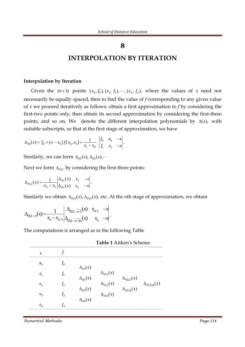
School of Distance Education
Numerical Methods Page 114
8
INTERPOLATION BY ITERATION
Interpolation by Iteration
Given the ( 1)n points 0 0 1 1( , ), ( , ), , ( , ),n nx f x f x f where the values of x need not
necessarily be equally spaced, then to find the value of f corresponding to any given valueof x we proceed iteratively as follows: obtain a first approximation to f by considering thefirst-two points only; then obtain its second approximation by considering the first-threepoints, and so on. We denote the different interpolation polynomials by ( ),x withsuitable subscripts, so that at the first stage of approximation, we have
01 0 0 0 1
1 0
1( ) ( ) [ , ]x f x x f x xx x
0 0
1 1
f x x
f x x.
Similarly, we can form 02 03( ), ( ),x x
Next we form 012 by considering the first-three points:
01 1
0122 1 02 2
( )1( )( )
x x xx
x x x x x.
Similarly we obtain 013 014( ), ( ),x x etc. At the nth stage of approximation, we obtain
1012 1012
1 012 2
( )1( )( )
nnn
n n nn n
x x xx
x x x x x .
The computations is arranged as in the following Table
Table 1 Aitken’s Scheme
x f
0x
1x
2x
3x
4x
0f
1f
2f
3f
4f
01( )x
02 ( )x
03( )x
04 ( )x
012 ( )x
013( )x
014 ( )x
0123( )x
0124 ( )x01234 ( )x
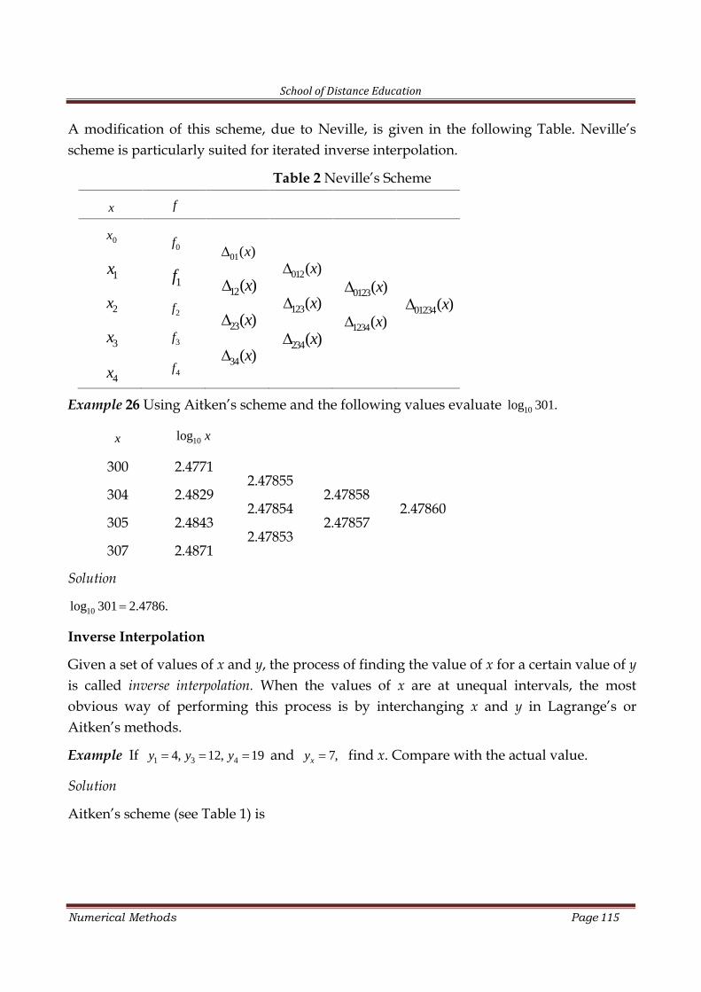
School of Distance Education
Numerical Methods Page 115
A modification of this scheme, due to Neville, is given in the following Table. Neville’sscheme is particularly suited for iterated inverse interpolation.
Table 2 Neville’s Scheme
x f
0x
1x
2x
3x
4x
0f
1f
2f
3f
4f
01( )x
12( )x
23( )x
34( )x
012( )x
123( )x
234( )x
0123( )x
1234( )x01234( )x
Example 26 Using Aitken’s scheme and the following values evaluate 10log 301.
x 10log x
300
304
305
307
2.4771
2.4829
2.4843
2.4871
2.47855
2.47854
2.47853
2.47858
2.478572.47860
Solution
10log 301 2.4786.
Inverse Interpolation
Given a set of values of x and y, the process of finding the value of x for a certain value of yis called inverse interpolation. When the values of x are at unequal intervals, the mostobvious way of performing this process is by interchanging x and y in Lagrange’s orAitken’s methods.
Example If 1 3 44, 12, 19y y y and 7,xy find x. Compare with the actual value.
Solution
Aitken’s scheme (see Table 1) is
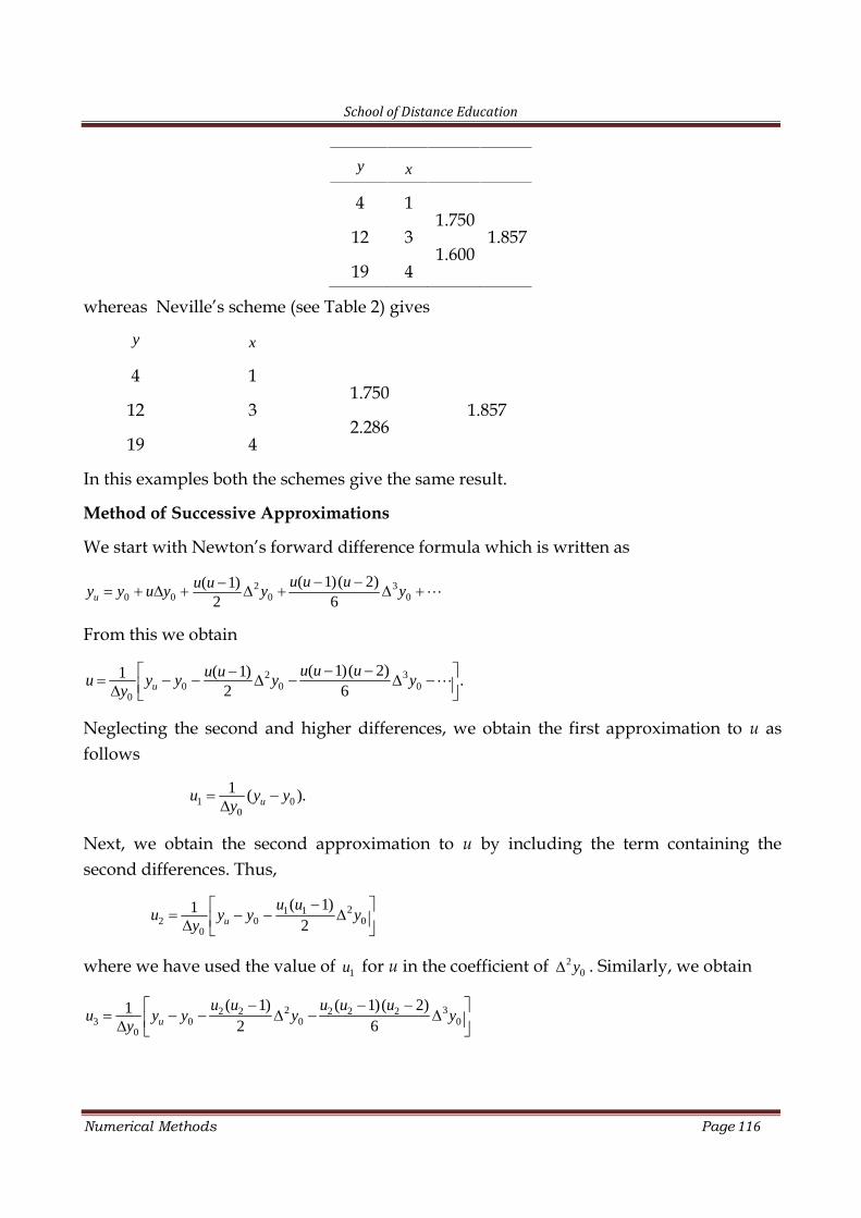
School of Distance Education
Numerical Methods Page 116
y x
4
12
19
1
3
4
1.750
1.6001.857
whereas Neville’s scheme (see Table 2) gives
y x
4
12
19
1
3
4
1.750
2.2861.857
In this examples both the schemes give the same result.
Method of Successive Approximations
We start with Newton’s forward difference formula which is written as
2 30 0 0 0
( 1)( 2)( 1)2 6u
u u uu uy y u y y y
From this we obtain
2 30 0 0
0
( 1)( 2)( 1)1 .2 6u
u u uu uu y y y yy
Neglecting the second and higher differences, we obtain the first approximation to u asfollows
1 00
1 ( ).uu y yy
Next, we obtain the second approximation to u by including the term containing thesecond differences. Thus,
21 1
2 0 00
( 1)12u
u uu y y y
y
where we have used the value of 1u for u in the coefficient of 20y . Similarly, we obtain
2 32 2 2 2 2
3 0 0 00
( 1) ( 1)( 2)12 6u
u u u u uu y y y y
y
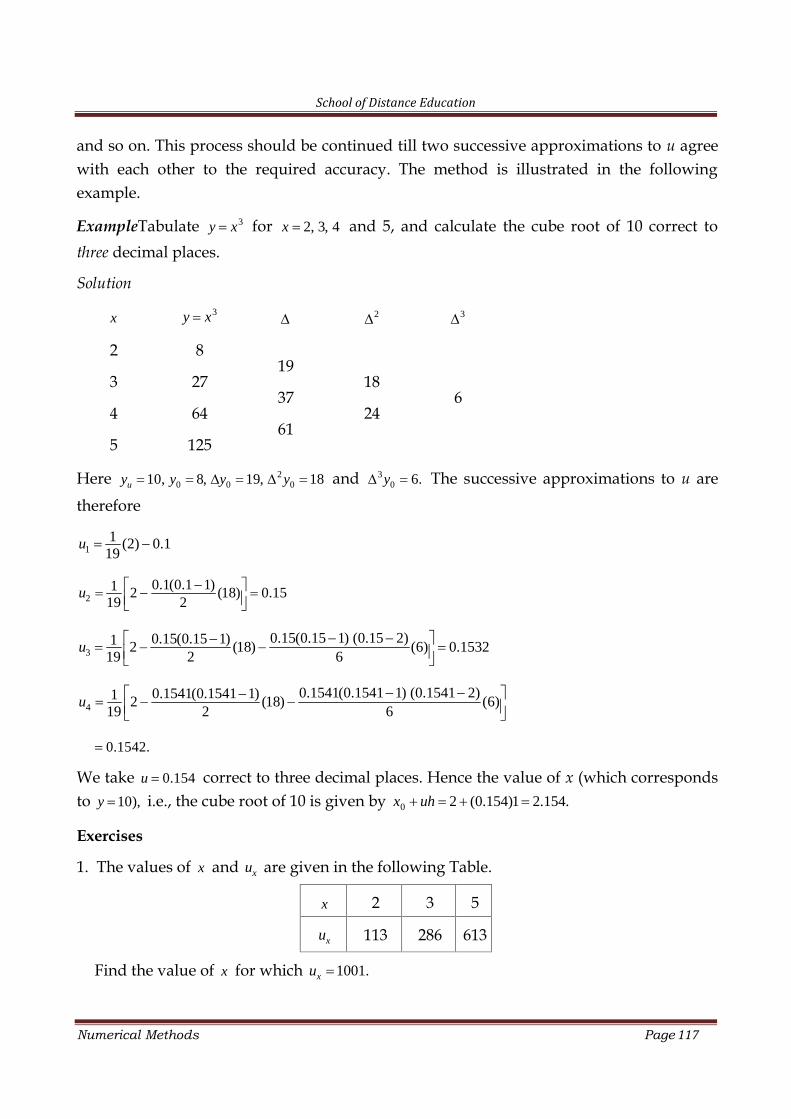
School of Distance Education
Numerical Methods Page 117
and so on. This process should be continued till two successive approximations to u agreewith each other to the required accuracy. The method is illustrated in the followingexample.
ExampleTabulate 3y x for 2, 3, 4x and 5, and calculate the cube root of 10 correct tothree decimal places.
Solution
x 3y x 2 3
2
3
4
5
8
27
64
125
19
37
61
18
246
Here 20 0 010, 8, 19, 18uy y y y and 3
0 6.y The successive approximations to u are
therefore
11 (2) 0.119
u
20.1(0.1 1)1 2 (18) 0.15
19 2u
30.15(0.15 1) (0.15 2)0.15(0.15 1)1 2 (18) (6) 0.1532
19 2 6u
40.1541(0.1541 1) (0.1541 2)0.1541(0.1541 1)1 2 (18) (6)
19 2 6u
0.1542.
We take 0.154u correct to three decimal places. Hence the value of x (which correspondsto 10),y i.e., the cube root of 10 is given by 0 2 (0.154)1 2.154.x uh
Exercises
1. The values of x and xu are given in the following Table.
x 2 3 5
xu 113 286 613
Find the value of x for which 1001.xu
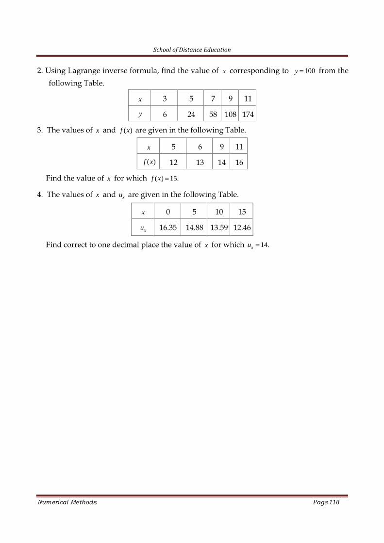
School of Distance Education
Numerical Methods Page 118
2. Using Lagrange inverse formula, find the value of x corresponding to 100y from thefollowing Table.
x 3 5 7 9 11
y 6 24 58 108 174
3. The values of x and ( )f x are given in the following Table.
x 5 6 9 11
( )f x 12 13 14 16
Find the value of x for which ( ) 15.f x
4. The values of x and xu are given in the following Table.
x 0 5 10 15
xu 16.35 14.88 13.59 12.46
Find correct to one decimal place the value of x for which 14.xu
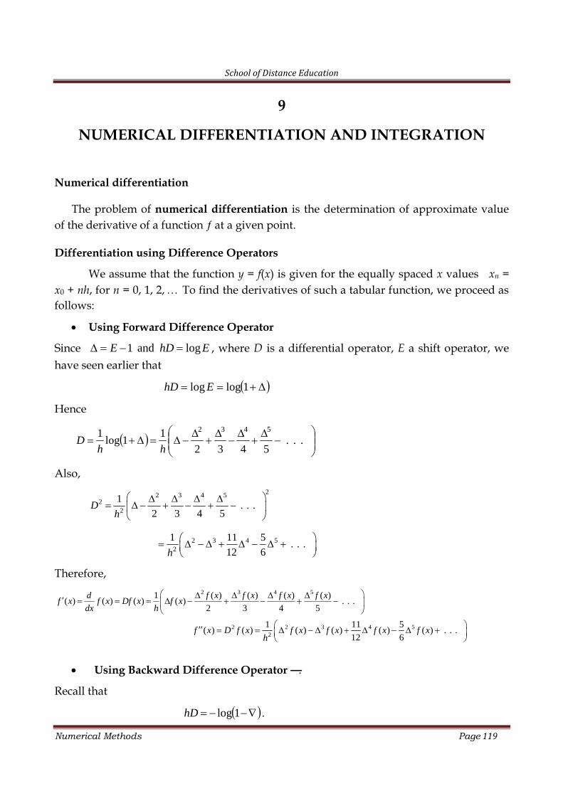
School of Distance Education
Numerical Methods Page 119
9
NUMERICAL DIFFERENTIATION AND INTEGRATION
Numerical differentiation
The problem of numerical differentiation is the determination of approximate valueof the derivative of a function at a given point.
Differentiation using Difference Operators
We assume that the function y = f(x) is given for the equally spaced x values xn =x0 + nh, for n = 0, 1, 2, To find the derivatives of such a tabular function, we proceed asfollows:
Using Forward Difference Operator
Since EhDE logand1 , where D is a differential operator, E a shift operator, wehave seen earlier that
1loglog EhD
Hence
...
5432
11log
1 5432
hhD
Also,22 3 4 5
22
1. . .
2 3 4 5
Dh
2 3 4 52
1 11 5. . .
12 6 h
Therefore,2 3 4 51 ( ) ( ) ( ) ( )
( ) ( ) ( ) ( ) . . .2 3 4 5
d f x f x f x f xf x f x Df x f x
dx h
2 2 3 4 52
1 11 5( ) ( ) ( ) ( ) ( ) ( ) . . .
12 6
f x D f x f x f x f x f xh
Using Backward Difference Operator .
Recall that
1loghD .
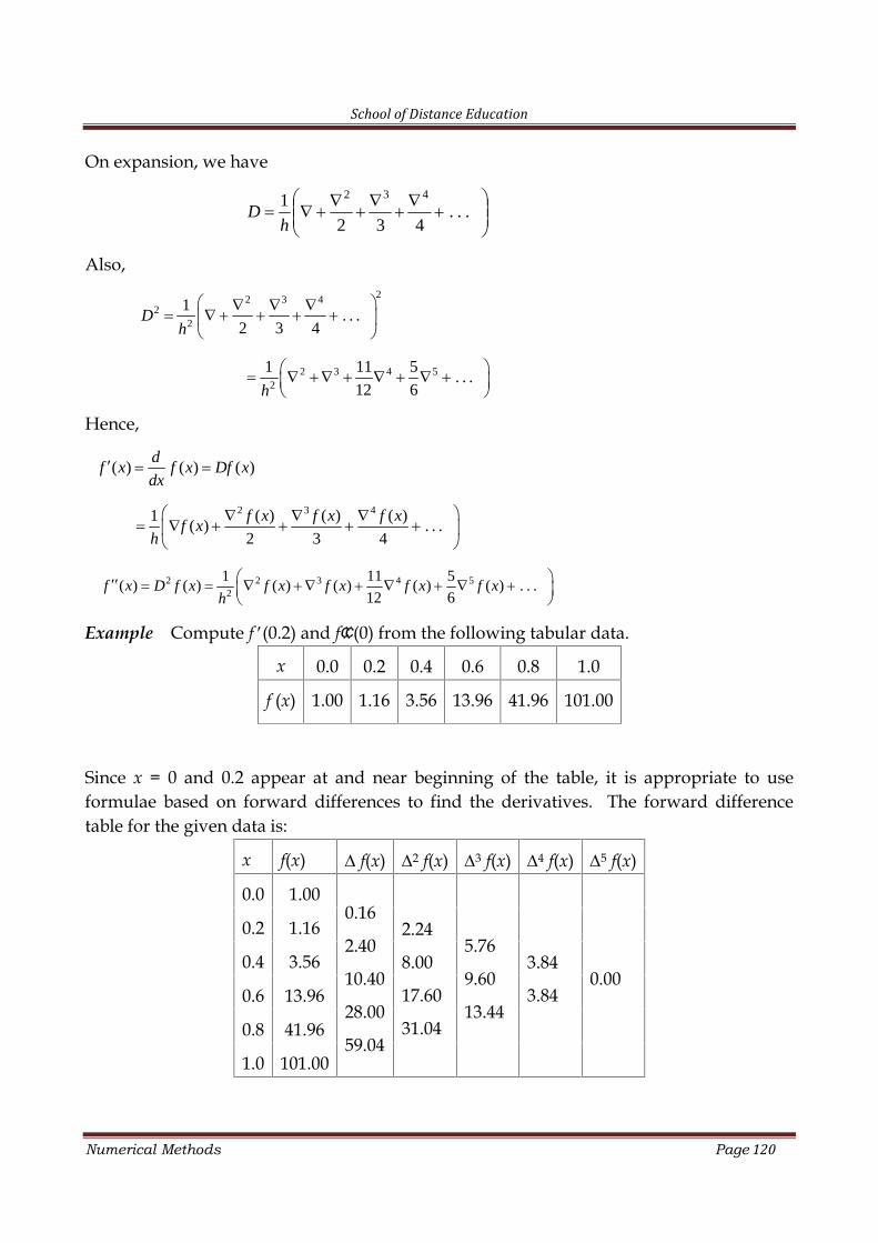
School of Distance Education
Numerical Methods Page 120
On expansion, we have
...
432
1 432
hD
Also,22 3 4
22
1. . .
2 3 4
Dh
2 3 4 52
1 11 5. . .
12 6 h
Hence,
( ) ( ) ( )d
f x f x Df xdx
2 3 41 ( ) ( ) ( )( ) . . .
2 3 4
f x f x f xf x
h
2 2 3 4 52
1 11 5( ) ( ) ( ) ( ) ( ) ( ) . . .
12 6f x D f x f x f x f x f x
h
Example Compute f (0.2) and f (0) from the following tabular data.
x 0.0 0.2 0.4 0.6 0.8 1.0
f (x) 1.00 1.16 3.56 13.96 41.96 101.00
Since x = 0 and 0.2 appear at and near beginning of the table, it is appropriate to useformulae based on forward differences to find the derivatives. The forward differencetable for the given data is:
x f(x) f(x) 2 f(x) 3 f(x) 4 f(x) 5 f(x)
0.0 1.000.16
2.40
10.40
28.00
59.04
2.24
8.00
17.60
31.04
5.76
9.60
13.44
3.84
3.840.00
0.2 1.16
0.4 3.56
0.6 13.96
0.8 41.96
1.0 101.00
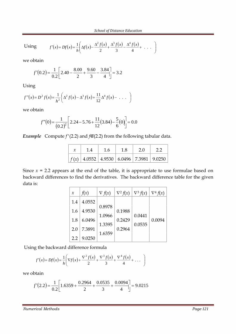
School of Distance Education
Numerical Methods Page 121
Using
...
432
1 432 xfxfxfxf
hxDfxf
we obtain
2.34
84.3
3
60.9
2
00.840.2
2.0
12.0
f
Using
...
12
111 4322
2 xfxfxfh
xfDxf
we obtain
0.006
584.3
12
1176.524.2
2.0
10
2
f
Example Compute f (2.2) and f (2.2) from the following tabular data.
x 1.4 1.6 1.8 2.0 2.2
f (x) 4.0552 4.9530 6.0496 7.3981 9.0250
Since x = 2.2 appears at the end of the table, it is appropriate to use formulae based onbackward differences to find the derivatives. The backward difference table for the givendata is:
x f(x) f(x) 2 f(x) 3 f(x) 4 f(x)
1.4 4.05520.8978
1.0966
1.3395
1.6359
0.1988
0.2429
0.2964
0.0441
0.05350.0094
1.6 4.9530
1.8 6.0496
2.0 7.3891
2.2 9.0250
Using the backward difference formula
...
432
1 432 xfxfxfxf
hxDfxf
we obtain
0215.94
0094.0
3
0535.0
2
2964.06359.1
2.0
12.2
f
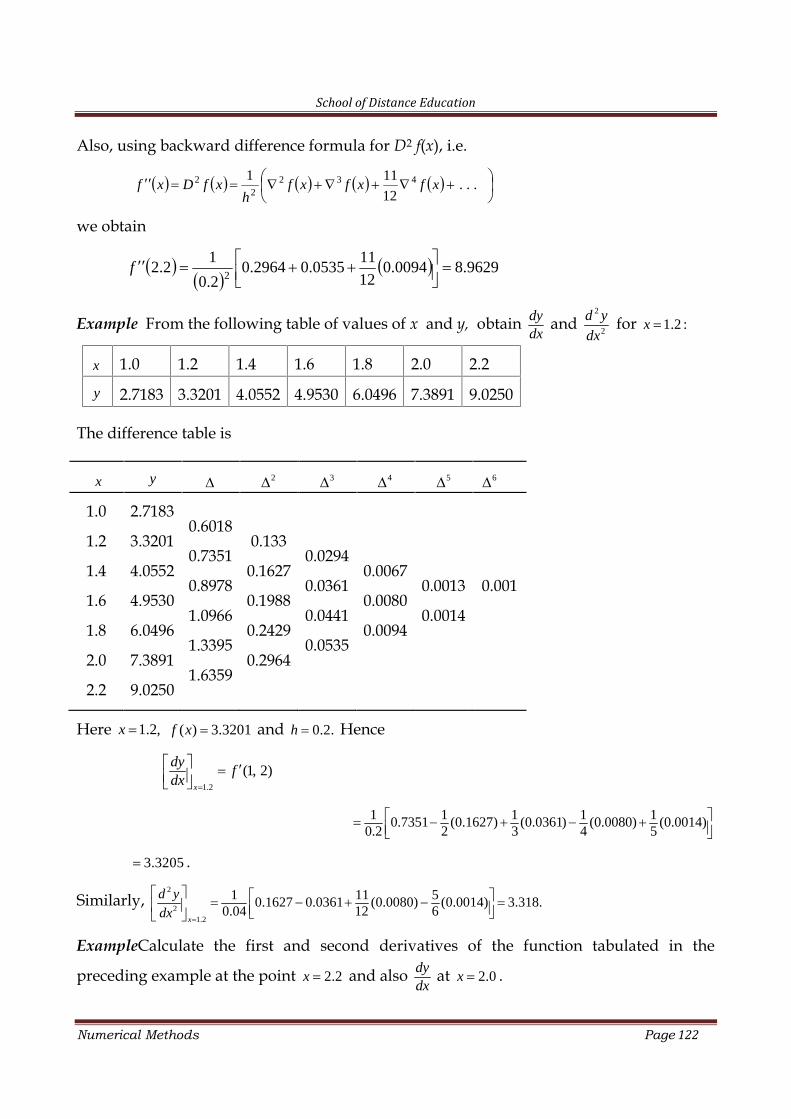
School of Distance Education
Numerical Methods Page 122
Also, using backward difference formula for D2 f(x), i.e.
...
12
111 4322
2 xfxfxfh
xfDxf
we obtain
9629.80094.012
110535.02964.0
2.0
12.2
2
f
Example From the following table of values of x and y, obtain dydx
and2
2
d y
dxfor 1.2 :x
x 1.0 1.2 1.4 1.6 1.8 2.0 2.2
y 2.7183 3.3201 4.0552 4.9530 6.0496 7.3891 9.0250
The difference table is
x y 2 3 4 5 6
1.0
1.2
1.4
1.6
1.8
2.0
2.2
2.7183
3.3201
4.0552
4.9530
6.0496
7.3891
9.0250
0.6018
0.7351
0.8978
1.0966
1.3395
1.6359
0.133
0.1627
0.1988
0.2429
0.2964
0.0294
0.0361
0.0441
0.0535
0.0067
0.0080
0.0094
0.0013
0.0014
0.001
Here 1.2,x ( ) 3.3201f x and 0.2.h Hence
1.2
(1, 2)x
dyf
dx
1 1 1 1 10.7351 (0.1627) (0.0361) (0.0080) (0.0014)0.2 2 3 4 5
3.3205 .
Similarly,2
21.2
1 11 50.1627 0.0361 (0.0080) (0.0014) 3.318.0.04 12 6
x
d y
dx
ExampleCalculate the first and second derivatives of the function tabulated in the
preceding example at the point 2.2x and also dydx
at 2.0x .
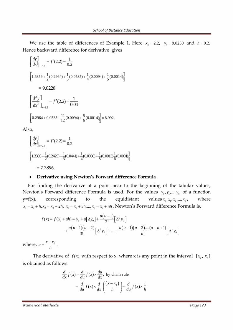
School of Distance Education
Numerical Methods Page 123
We use the table of differences of Example 1. Here 2.2,nx 9.0250ny and 0.2.h
Hence backward difference for derivative gives
2.2
1(2.2)0.2
x
dyf
dx
1 1 1 11.6359 (0.2964) (0.0535) (0.0094) (0.0014)2 3 4 5
= 9.0228.
2
22.2
1(2.2)0.04
x
d yf
dx
11 50.2964 0.0535 (0.0094) (0.0014) 8.992.12 6
Also,
2.0
1(2.2)0.2
x
dyf
dx
1 1 1 1 11.3395 (0.2429) (0.0441) (0.0080) (0.0013) (0.0001)2 3 4 5 6
= 7.3896.
Derivative using Newton’s Forward difference Formula
For finding the derivative at a point near to the beginning of the tabular values,Newton’s Forward difference Formula is used. For the values 0 1, ,..., ny y y of a functiony=f(x), corresponding to the equidistant values 0 1 2, , ,..., nx x x x , where
1 0 2 0 3 0 0, 2 , 3 ,..., nx x h x x h x x h x x nh , Newton’s Forward difference Formula is,
20 0 0 0
30 0
1( ) ( )
2!1 2 1 2 ....( 1)
....3! !
n
u uf x f x uh y u y y
u u u u u u u ny y
n
where, 0x xu
h
.
The derivative of ( )f x with respect to x, where x is any point in the interval 0[ , ]nx x
is obtained as follows:
0
( ) ( ) , by chain rule
1( ) ( )
d d duf x f xdx du dx
x xd d df x f xdu dx h du h
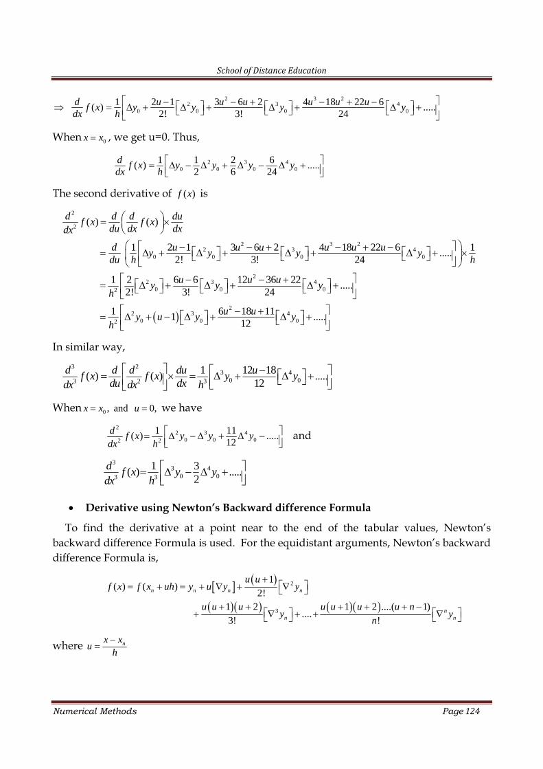
School of Distance Education
Numerical Methods Page 124
2 3 22 3 4
0 0 0 01 2 1 3 6 2 4 18 22 6( ) .....
2! 3! 24d u u u u u uf x y y y ydx h
When 0x x , we get u=0. Thus,
2 3 40 0 0 0
1 1 2 6( ) .....2 6 24
d f x y y y ydx h
The second derivative of ( )f x is
2
2
2 3 22 3 4
0 0 0 0
22 3 4
0 0 02
2 30 02
( ) ( )
1 2 1 3 6 2 4 18 22 6 1.....2! 3! 24
1 2 6 6 12 36 22 .....2! 3! 24
1 1
d d d duf x f xdu dx dxdx
d u u u u u uy y y ydu h h
u u uy y yh
y u yh
2
40
6 18 11 .....12
u u y
In similar way,3 2
3 40 03 2 3
1 12 18( ) ( ) .....12
d d d du uf x f x y ydu dxdx dx h
When 0 , and 0,x x u we have2
2 3 40 0 02 2
1 11( ) .....12
d f x y y ydx h
and
33 4
0 03 3
1 3( ) .....2
d f x y ydx h
Derivative using Newton’s Backward difference Formula
To find the derivative at a point near to the end of the tabular values, Newton’sbackward difference Formula is used. For the equidistant arguments, Newton’s backwarddifference Formula is,
2
3
1( ) ( )
2!1 2 1 2 ....( 1)
....3! !
n n n n
nn n
u uf x f x uh y u y y
u u u u u u u ny y
n
where nx xu
h
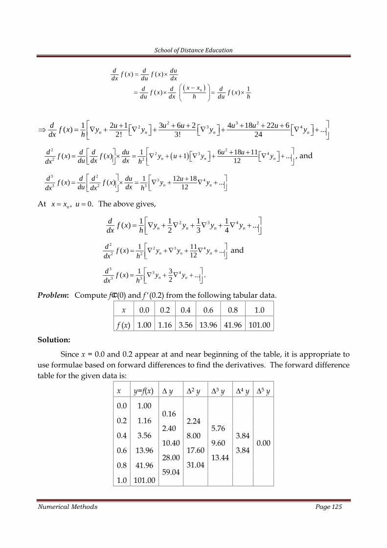
School of Distance Education
Numerical Methods Page 125
( ) ( )
1( ) ( )n
d d duf x f xdx du dx
x xd d df x f xdu dx h du h
2 3 22 3 41 2 1 3 6 2 4 18 22 6( ) ...
2! 3! 24n n n nd u u u u u uf x y y y ydx h
2 2
2 3 42 2
1 6 18 11( ) ( ) 1 ...12n n n
d d d du u uf x f x y u y ydu dx dxdx h
, and
3 23 4
3 2 3
1 12 18( ) ( ) ...12n n
d d d du uf x f x y ydu dxdx dx h
At , 0.nx x u The above gives,
2 3 41 1 1 1( ) ...2 3 4n n n n
d f x y y y ydx h
2
2 3 42 2
1 11( ) ...12n n n
d f x y y ydx h
and
33 4
3 3
1 3( ) ...2n n
d f x y ydx h
.
Problem: Compute f (0) and f (0.2) from the following tabular data.
x 0.0 0.2 0.4 0.6 0.8 1.0
f (x) 1.00 1.16 3.56 13.96 41.96 101.00
Solution:
Since x = 0.0 and 0.2 appear at and near beginning of the table, it is appropriate touse formulae based on forward differences to find the derivatives. The forward differencetable for the given data is:
x y=f(x) y 2 y 3 y 4 y 5 y
0.0 1.000.16
2.40
10.40
28.00
59.04
2.24
8.00
17.60
31.04
5.76
9.60
13.44
3.84
3.840.00
0.2 1.16
0.4 3.56
0.6 13.96
0.8 41.96
1.0 101.00
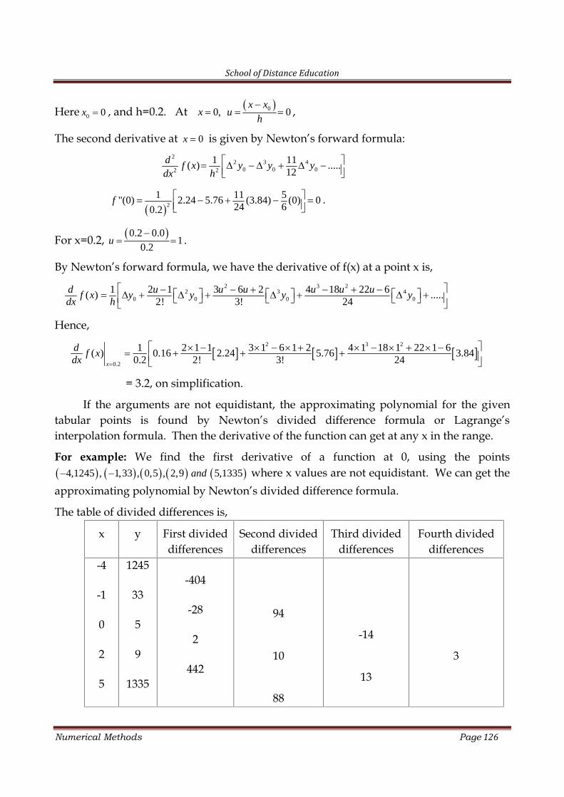
School of Distance Education
Numerical Methods Page 126
Here 0 0x , and h=0.2. At 00, 0x x
x uh
,
The second derivative at 0x is given by Newton’s forward formula:2
2 3 40 0 02 2
1 11( ) .....12
d f x y y ydx h
21 11 5"(0) 2.24 5.76 (3.84) (0) 0
24 60.2f
.
For x=0.2, 0.2 0.01
0.2u
.
By Newton’s forward formula, we have the derivative of f(x) at a point x is,2 3 2
2 3 40 0 0 0
1 2 1 3 6 2 4 18 22 6( ) .....2! 3! 24
d u u u u u uf x y y y ydx h
Hence,
2 3 2
0.2
1 2 1 1 3 1 6 1 2 4 1 18 1 22 1 6( ) 0.16 2.24 5.76 3.840.2 2! 3! 24x
d f xdx
= 3.2, on simplification.
If the arguments are not equidistant, the approximating polynomial for the giventabular points is found by Newton’s divided difference formula or Lagrange’sinterpolation formula. Then the derivative of the function can get at any x in the range.
For example: We find the first derivative of a function at 0, using the points 4,1245 , 1,33 , 0,5 , 2,9 5,1335and where x values are not equidistant. We can get theapproximating polynomial by Newton’s divided difference formula.
The table of divided differences is,
x y First divideddifferences
Second divideddifferences
Third divideddifferences
Fourth divideddifferences
-4
-1
0
2
5
1245
33
5
9
1335
-404
-28
2
442
94
10
88
-14
13
3
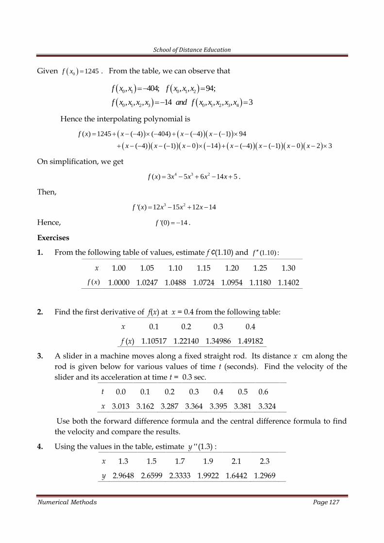
School of Distance Education
Numerical Methods Page 127
Given 0 1245f x . From the table, we can observe that
0 1 0 1 2
0 1 2 3 0 1 2 3 4
, 404; , , 94;
, , , 14 , , , , 3
f x x f x x x
f x x x x and f x x x x x
Hence the interpolating polynomial is
( ) 1245 ( 4) ( 404) ( 4) ( 1) 94
( 4) ( 1) 0 14 ( 4) ( 1) 0 2 3
f x x x x
x x x x x x x
On simplification, we get4 3 2( ) 3 5 6 14 5f x x x x x .
Then,3 2'( ) 12 15 12 14f x x x x
Hence, '(0) 14f .
Exercises
1. From the following table of values, estimate f (1.10) and (1.10) :f
x 1.00 1.05 1.10 1.15 1.20 1.25 1.30
( )f x 1.0000 1.0247 1.0488 1.0724 1.0954 1.1180 1.1402
2. Find the first derivative of f(x) at x = 0.4 from the following table:
x 0.1 0.2 0.3 0.4
f (x) 1.10517 1.22140 1.34986 1.49182
3. A slider in a machine moves along a fixed straight rod. Its distance x cm along therod is given below for various values of time t (seconds). Find the velocity of theslider and its acceleration at time t = 0.3 sec.
t 0.0 0.1 0.2 0.3 0.4 0.5 0.6
x 3.013 3.162 3.287 3.364 3.395 3.381 3.324
Use both the forward difference formula and the central difference formula to findthe velocity and compare the results.
4. Using the values in the table, estimate y (1.3) :
x 1.3 1.5 1.7 1.9 2.1 2.3
y 2.9648 2.6599 2.3333 1.9922 1.6442 1.2969
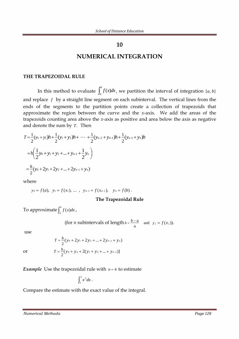
School of Distance Education
Numerical Methods Page 128
10
NUMERICAL INTEGRATION
THE TRAPEZOIDAL RULE
In this method to evaluate ( )b
af x dx , we partition the interval of integration [ , ]a b
and replace f by a straight line segment on each subinterval. The vertical lines from theends of the segments to the partition points create a collection of trapezoids thatapproximate the region between the curve and the x-axis. We add the areas of thetrapezoids counting area above the x-axis as positive and area below the axis as negativeand denote the sum by .T Then
0 1 1 2 2 1 11 1 1 1(2 2 2 2
) ( ) ( ) ( )n n n nT y y h y y h y y h y y h
0 1 2 11 1...2 2
n nh y y y y y
0 1 2 12
( 2 2 ... 2 )n nh y y y y y
where
( ), ( ), ... , ( ), ( )0 1 1 1 1 n n ny f a y f x y f x y f b .
The Trapezoidal Rule
To approximate ( )b
af x dx ,
(for n subintervals of length h
b a
nand ( )).j jy f x
use
0 1 2 12
( 2 2 ... 2 ) n nhT y y y y y
or 0 1 2 12
[ 2( ... )] n nhT y y y y y
Example Use the trapezoidal rule with 4n to estimate2 2
1x dx .
Compare the estimate with the exact value of the integral.
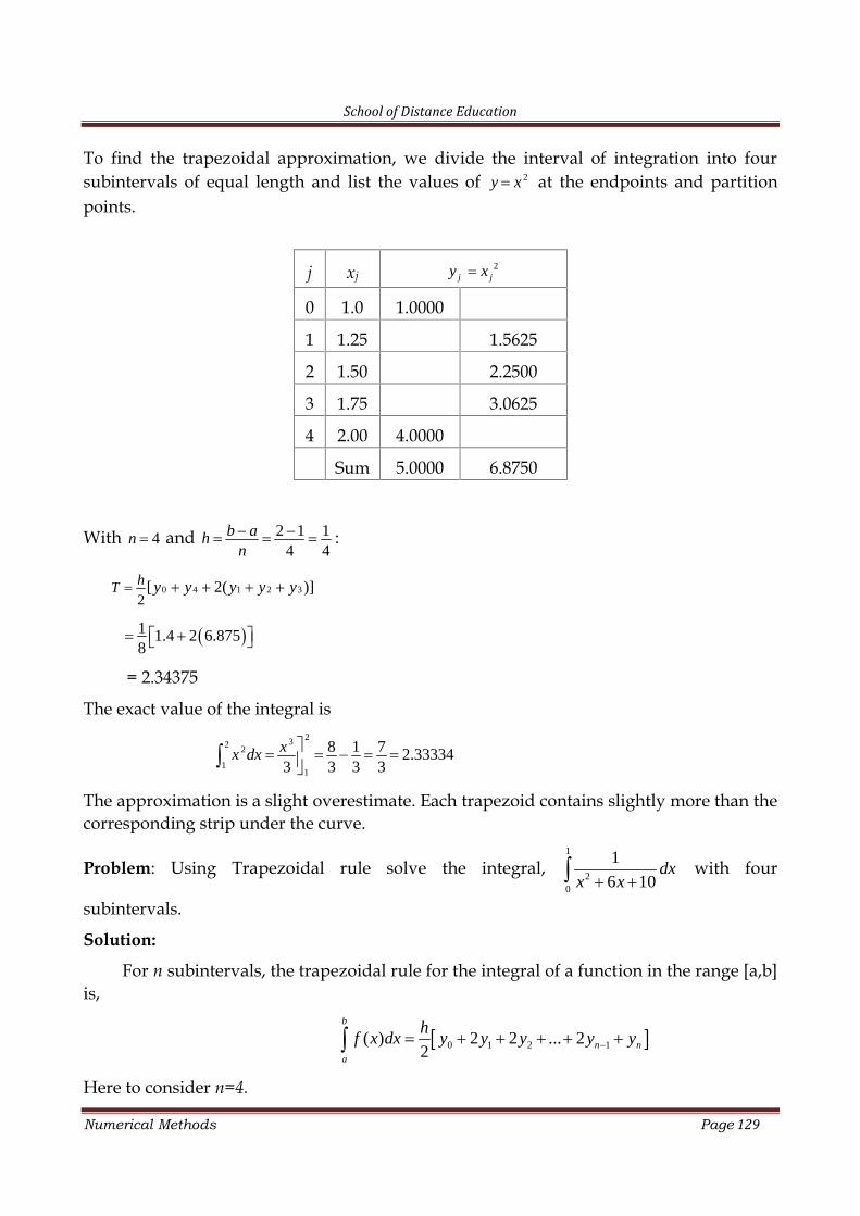
School of Distance Education
Numerical Methods Page 129
To find the trapezoidal approximation, we divide the interval of integration into foursubintervals of equal length and list the values of 2y x at the endpoints and partitionpoints.
j xj2j jy x
0 1.0 1.0000
1 1.25 1.5625
2 1.50 2.2500
3 1.75 3.0625
4 2.00 4.0000
Sum 5.0000 6.8750
With 4n and 2 1 14 4
b ahn :
0 4 1 2 32
[ 2( )] hT y y y y y
1 1.4 2 6.8758
= 2.34375
The exact value of the integral is232 2
11
8 1 7 2.333343 3 3 3xx dx
The approximation is a slight overestimate. Each trapezoid contains slightly more than thecorresponding strip under the curve.
Problem: Using Trapezoidal rule solve the integral,1
20
1
6 10dx
x x with four
subintervals.
Solution:
For n subintervals, the trapezoidal rule for the integral of a function in the range [a,b]is,
0 1 2 1( ) 2 2 ... 22 n n
b
a
hf x dx y y y y y
Here to consider n=4.
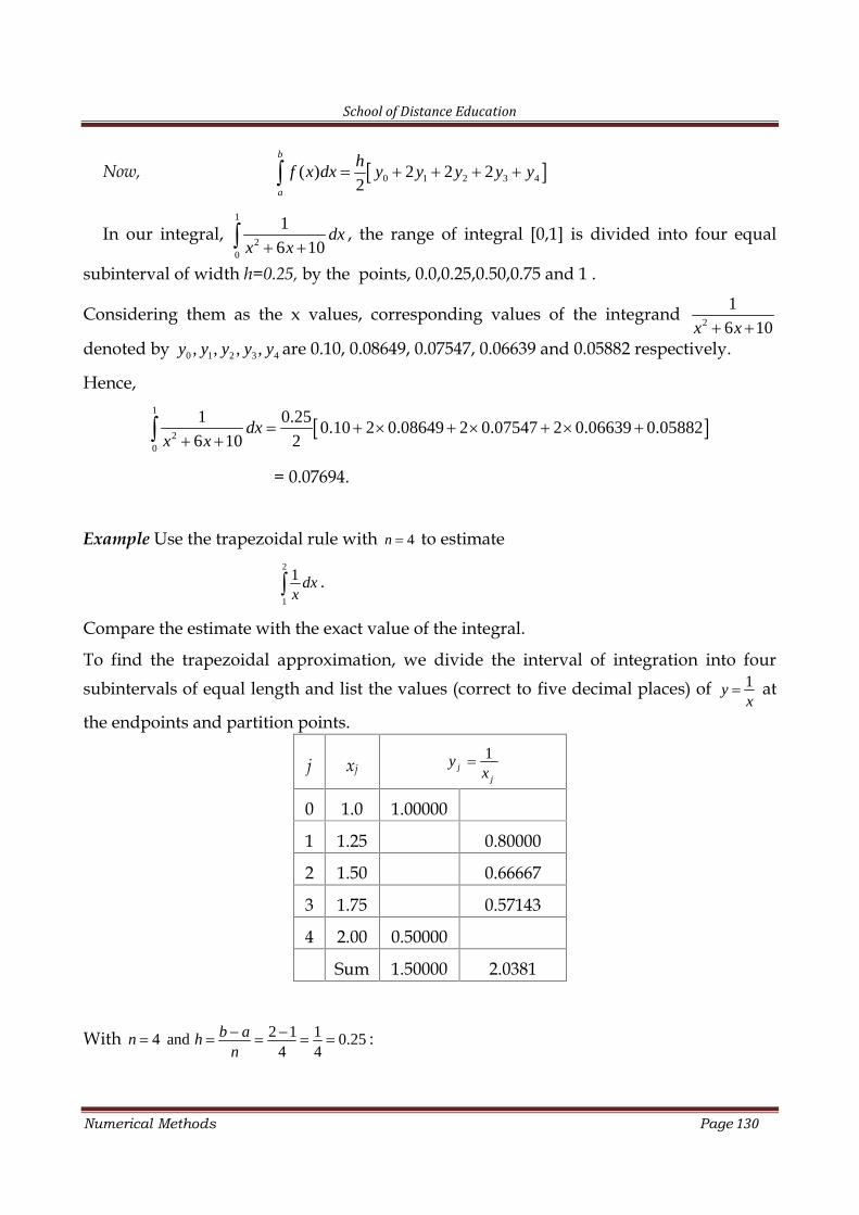
School of Distance Education
Numerical Methods Page 130
Now, 0 1 2 3 4( ) 2 2 22
b
a
hf x dx y y y y y
In our integral,1
20
1
6 10dx
x x , the range of integral [0,1] is divided into four equal
subinterval of width h=0.25, by the points, 0.0,0.25,0.50,0.75 and 1 .
Considering them as the x values, corresponding values of the integrand2
1
6 10x x denoted by 0 1 2 3 4, , , ,y y y y y are 0.10, 0.08649, 0.07547, 0.06639 and 0.05882 respectively.
Hence,
1
20
1 0.250.10 2 0.08649 2 0.07547 2 0.06639 0.05882
6 10 2dx
x x
= 0.07694.
Example Use the trapezoidal rule with 4n to estimate2
1
1 dxx
.
Compare the estimate with the exact value of the integral.
To find the trapezoidal approximation, we divide the interval of integration into foursubintervals of equal length and list the values (correct to five decimal places) of 1y
xat
the endpoints and partition points.
j xj1j
j
yx
0 1.0 1.00000
1 1.25 0.80000
2 1.50 0.66667
3 1.75 0.57143
4 2.00 0.50000
Sum 1.50000 2.0381
With 2 1 14 and 0.254 4
b an hn
:
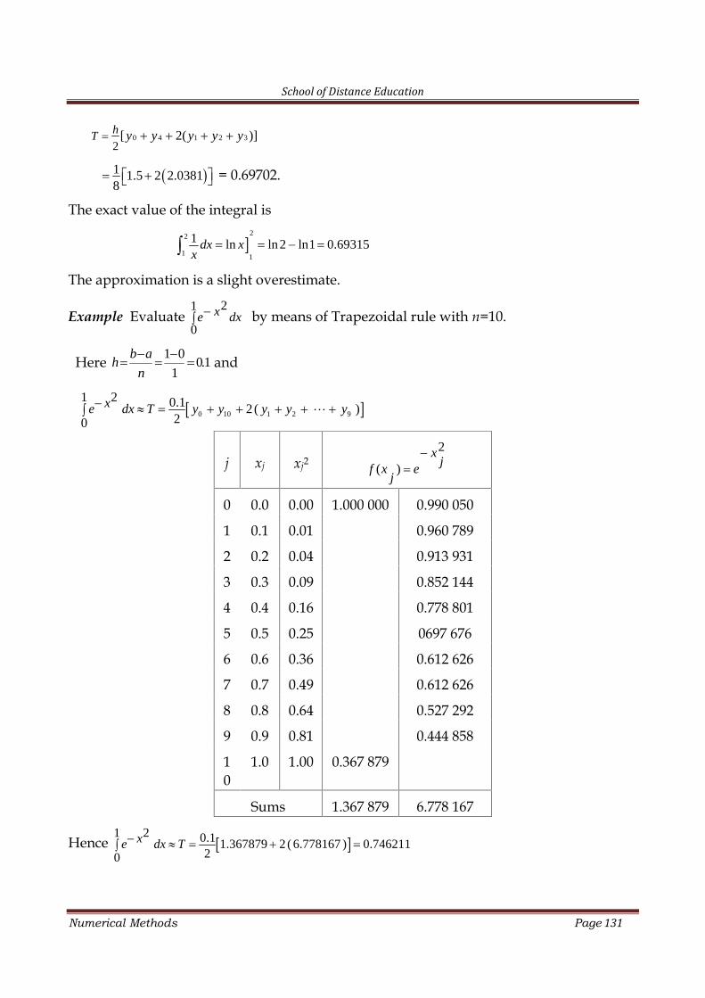
School of Distance Education
Numerical Methods Page 131
0 4 1 2 32
[ 2( )] hT y y y y y
1 1.5 2 2.03818 = 0.69702.
The exact value of the integral is
22
1 1
1 ln ln2 ln1 0.69315dx xx
The approximation is a slight overestimate.
Example Evaluate 1
0
2dxxe by means of Trapezoidal rule with n=10.
Here 1.01
01
n
abh and
0 10 1 2 9
21 0.1 2( )20
xe dx T y y y y y
j xj xj22
)(j
xe
jxf
0 0.0 0.00 1.000 000 0.990 050
1 0.1 0.01 0.960 789
2 0.2 0.04 0.913 931
3 0.3 0.09 0.852 144
4 0.4 0.16 0.778 801
5 0.5 0.25 0697 676
6 0.6 0.36 0.612 626
7 0.7 0.49 0.612 626
8 0.8 0.64 0.527 292
9 0.9 0.81 0.444 858
10
1.0 1.00 0.367 879
Sums 1.367 879 6.778 167
Hence 21 0.1 1.367879 2 ( 6.778167 ) 0.746211
20
xe dx T
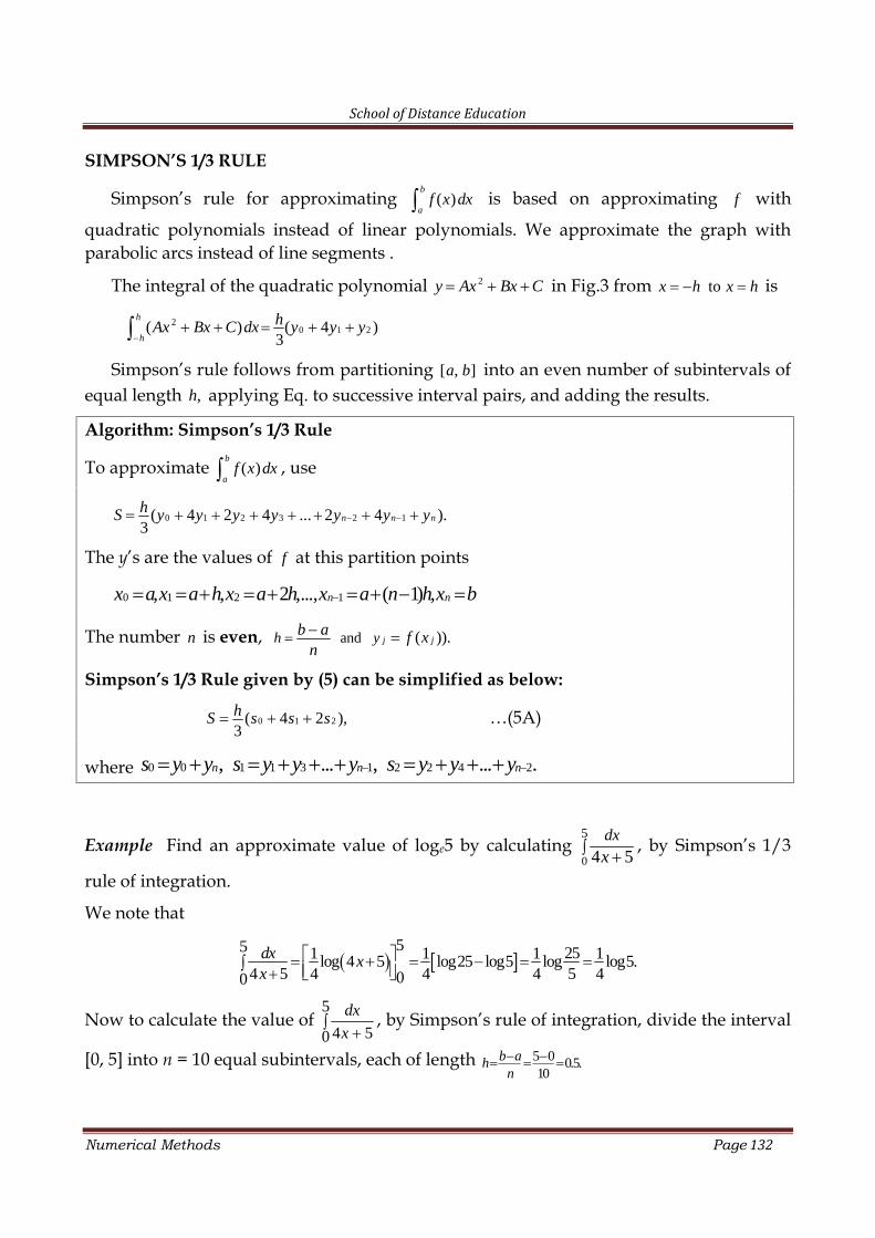
School of Distance Education
Numerical Methods Page 132
SIMPSON’S 1/3 RULE
Simpson’s rule for approximating ( )b
af x dx is based on approximating f with
quadratic polynomials instead of linear polynomials. We approximate the graph withparabolic arcs instead of line segments .
The integral of the quadratic polynomial 2y Ax Bx C in Fig.3 from tox h x h is
20 1 2( ) ( 4 )
3
h
h
hAx Bx C dx y y y
Simpson’s rule follows from partitioning [ , ]a b into an even number of subintervals ofequal length ,h applying Eq. to successive interval pairs, and adding the results.
Algorithm: Simpson’s 1/3 Rule
To approximate ( )b
af x dx , use
0 1 2 3 2 1( 4 2 4 ... 2 4 ).3
n n nhS y y y y y y y
The y’s are the values of f at this partition points
0 1 2 1, , 2 ,..., ( 1) ,n nx a x a h x a h x a n h x b
The number n is even, and ( )).j jh yb a f xn
Simpson’s 1/3 Rule given by (5) can be simplified as below:
0 1 2( 4 2 ),3hS s s s …(5A)
where 0 0 1 1 3 1 2 2 4 2, ... , ... .n n ns y y s y y y s y y y
Example Find an approximate value of loge5 by calculating0
5
4 5dx
x , by Simpson’s 1/3
rule of integration.
We note that
55 251 1 1 1log 4 5 log25 log5 log log5.
4 5 4 4 4 5 400
dx xx
Now to calculate the value of
5
0 54x
dx , by Simpson’s rule of integration, divide the interval
[0, 5] into n = 10 equal subintervals, each of length 5 0 0.5.10
b ahn
School of Distance Education
Numerical Methods Page 133
j xj4 xj+5
1( )4 5
j jj
f f xx
0 0.0 5 0.20
1 0.5 7 0.1429
2 1.0 9 0.1111
3 1.5 11 0.0909
4 2.0 13 0.0769
5 2.5 15 0.6666
6 3.0 17 0.0588
7 3.5 19 0.0526
8 4.0 21 0.0476
9 4.5 23 0.0434
10 5.0 25 0.04
Sums s0=0.24 s1=0.3963 s2=0.2944
Hence,
.4023.0)2944.0(2)3963.0(424.03
5.05
0 54
S
x
dx
and loge 5 = 4(0.4023) = 1.6092.
Problem: Find10
20
1
1dx
x using Simpson’s one third rule.
Solution:
By Simpson’s one third rule, 0 1 3 2 4( ) 4 ... 2 ....3
b
n
a
hf x dx y y y y y y
In our integral,10
20
1
1dx
x , let the range [0,10] is subdivided into 10 equal interval of
width h=1, by the x values 0,1,2,3,4,5,6,7,8,9 and 10. Corresponding y values of the
function2
1
1 xare listed below:
Thus,
x 0 1 2 3 4 5 6 7 8 9 10
y 1 0.5 0.2 0.1 0.0588 0.0385 0.0270 0.02 0.0154 0.0122 0.0099
School of Distance Education
Numerical Methods Page 134
10
20
1 11 4 0.5 0.1 0.0385 0.02 0.0122 2 0.2 0.0588 0.027 0.0154 0.0099
1 3dx
x
11.0099 4 0.6707 2 0.3012
3
14.2951 1.4317
3 .
Problem: Evaluate6
20
1
3dx
x using Simpson’s three eight rule.
Solution:
By Simpson’s three eight rule,
0 1 2 4 1 3 6 9
3( ) 3 .... 2 ...
8 n n
b
a
hf x dx y y y y y y y y y
Let the limit of integral [0,6] be divided into six equal parts with interval h=1, using the
x values 0,1,2,3,4,5 and 6. Corresponding y values of the given integrand function2
1
3 xare,
Thus,
6
0 1 2 4 1 3 6 920
1 3 13 .... 2 ...
3 8 n ndx y y y y y y y y yx
For n=6,
6
0 1 2 4 5 3 620
1 3 13 2
3 8dx y y y y y y y
x
6
20
1 3 10.333 3 0.25 0.1429 0.0526 0.0357 2 0.1 0.0256
3 8dx
x
3 30.333 1.4436 0.2 0.0256 2.0022
8 8
6
20
10.7508
3dx
x
.
Example Find an approximation value of 21
0x dx by Simpson’s 1/3 rule with n = 10.
x 0 1 2 3 4 5 6
y 0.333 0.25 0.1429 0.1 0.0526 0.0357 0.0256
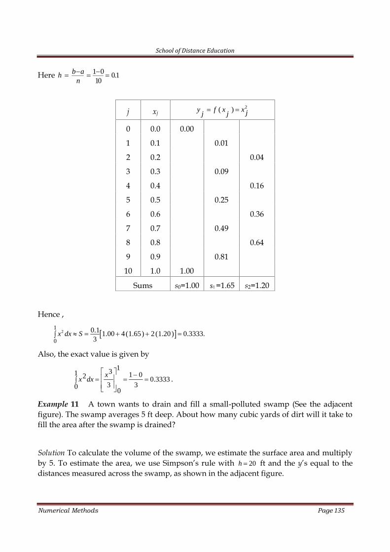
School of Distance Education
Numerical Methods Page 135
Here 1 0 0.110
b ahn
j xj2( )y f x x jj j
0 0.0 0.00
1 0.1 0.01
2 0.2 0.04
3 0.3 0.09
4 0.4 0.16
5 0.5 0.25
6 0.6 0.36
7 0.7 0.49
8 0.8 0.64
9 0.9 0.81
10 1.0 1.00
Sums s0=1.00 1s =1.65 s2=1.20
Hence ,
21
0
0.1 1.00 4(1.65) 2(1.20) 0.3333.3
x dx S
Also, the exact value is given by
3333.03
011
03
31
0
2
xdxx .
Example 11 A town wants to drain and fill a small-polluted swamp (See the adjacentfigure). The swamp averages 5 ft deep. About how many cubic yards of dirt will it take tofill the area after the swamp is drained?
Solution To calculate the volume of the swamp, we estimate the surface area and multiplyby 5. To estimate the area, we use Simpson’s rule with 20h ft and the y’s equal to thedistances measured across the swamp, as shown in the adjacent figure.
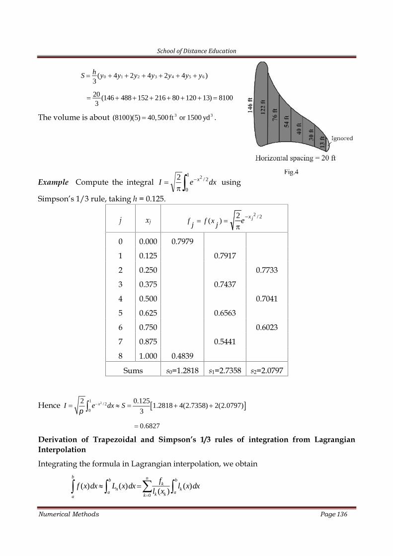
School of Distance Education
Numerical Methods Page 136
0 1 2 3 4 5 6( 4 2 4 2 4 )3hS y y y y y y y
20 (146 488 152 216 80 120 13) 81003
The volume is about ft or yd 3 3(8100)(5) 40,500 1500 .
Example Compute the integral
1
0
2/22dxeI x using
Simpson’s 1/3 rule, taking h = 0.125.
j xj2/22
)( jxe
jxf
jf
0 0.000 0.7979
1 0.125 0.7917
2 0.250 0.7733
3 0.375 0.7437
4 0.500 0.7041
5 0.625 0.6563
6 0.750 0.6023
7 0.875 0.5441
8 1.000 0.4839
Sums s0=1.2818 s1=2.7358 s2=2.0797
Hence 21/ 2
0
2 0.1251.2818 4(2.7358) 2(2.0797)
3 xI e dx S
0.6827
Derivation of Trapezoidal and Simpson’s 1/3 rules of integration from LagrangianInterpolation
Integrating the formula in Lagrangian interpolation, we obtain
0
( ) ( ) ( )( )
b nb bk
n ka ak kka
ff x dx L x dx l x dx
l x
School of Distance Education
Numerical Methods Page 137
For n = 1, we have only one interval [x0, x1] such that a = x0 and b = x1 and then theabove integration formula gives trapezoidal rule.
For n = 2 , we have two subintervals [x0, x1] and [x1, x2] of equal width h such that a= x0 and b = x2 and then the above integration formula becomes
2
00 1 2( ) ( ) 4
3
bx
xa
hf x dx f x dx f f f ,
and is the Simpson’s 1/3 rule of integration.
For n = 3 the above integration formula (4) becomes
3
00 1 2 3
3( ) ( ) 3 38
bx
xa
f x dx f x dx h f f f f ,
and is known as Simpson’s 3/8 rule of integration.
Simpson’s three eight (3/8) rule
When n=3, all the differences of order four or higher becomes zero.
Hence,
2 3 2 4
2 3 2 30 0 0 0
33 0
0
3 1 3 3 1 3( ) 3 3 3 0
2 2 3 2 6 4
x x h
x
f x dx h y y y y
0 1 0 2 1 0 3 2 1 0
9 1 27 9 1 813 2 27 9 3 3
2 2 3 2 6 4h y y y y y y y y y y
0 1 0 2 1 0 3 2 1 0
0 1 2 3
72 108 54 2 9 3 324
9 27 27 924
hy y y y y y y y y y
hy y y y
0 1 2 3
33 0
0
3( ) 3 3
8
x x h
x
hf x dx y y y y
Similarly, 3 4 5 6
66 0
3
3( ) 3 3
8
x x h
x
hf x dx y y y y
Finally, under the assumption that n is a multiple of three,
School of Distance Education
Numerical Methods Page 138
3 2 1
0
3
3( ) 3 3
8 n n n n
x x nhn
xn
hf x dx y y y y
Adding these integrals, we get,
0 1 2 3 3 4 5 6 3 2 1
0
3( ) 3 3 3 3 ... 3 3
8
x
n n n n
n
x
hf x dx y y y y y y y y y y y y
That is,
0 1 2 3 3 4 5 6 3 2 1
3( ) 3 3 3 3 ... 3 3
8 n n n n
b
a
hf x dx y y y y y y y y y y y y
0 1 2 3 4 5 6 7 1
3( ) 3 3 2 3 3 2 3 ... 3
8 n n
b
a
hf x dx y y y y y y y y y y
0 1 2 4 1 3 6 9
3( ) 3 .... 2 ...
8 n n
b
a
hf x dx y y y y y y y y y
Exercises
Estimate the integral using
(a) trapezoidal rule and (b) Simpson’s 1/3 rule.
1. 2
21
1S
ds 2.0
sin t dt
3.2 3
0x dx
4.2
1x dx 5.
1 2
1( 1)x dx
6.
2 3
0( )t t dt
7. 1
0
sindx
x
x 8. 1
0 1
1dx
x9.
6
021
1dx
x
10.1
0
ln 2dxx
11. dxx
7
1
1 12.3
1(2 1)x dx
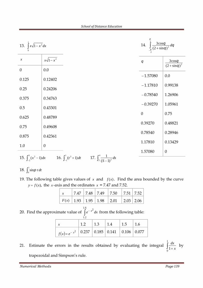
School of Distance Education
Numerical Methods Page 139
15.0 2
2( 1)x dx
16.
1 3
1( 1)t dt
17.
4
22
1( 1)
dsS
18.1
0sin t dt
19. The following table gives values of x and ( )f x . Find the area bounded by the curve( ),y f x the x -axis and the ordinates x = 7.47 and 7.52.
x 7.47 7.48 7.49 7.50 7.51 7.52
( )F x 1.93 1.95 1.98 2.01 2.03 2.06
20. Find the approximate value of 6.1
2.1
2dxe x from the following table:
x 1.2 1.3 1.4 1.5 1.6
2xexf 0.237 0.185 0.141 0.106 0.077
21. Estimate the errors in the results obtained by evaluating the integral 1
01 x
dx by
trapezoidal and Simpson’s rule.
14.2
2
2
3cos(2 sin )
d
2
3cos(2 sin )
1.57080 0.0
1.17810 0.99138
0.78540 1.26906
0.39270 1.05961
0 0.75
0.39270 0.48821
0.78540 0.28946
1.17810 0.13429
1.57080 0
13.1
2
0
1x x dx
x 21x x
0 0.0
0.125 0.12402
0.25 0.24206
0.375 0.34763
0.5 0.43301
0.625 0.48789
0.75 0.49608
0.875 0.42361
1.0 0
School of Distance Education
Numerical Methods Page 140
11
SOLUTION OF SYSTEMS OF LINEAR EQUATIONS
Solution of system of linear equations
A system of m linear equations in n unknowns x1, x2, . . . , xn is a set of equations ofthe form
a1 1 x1 + a1 2 x2 + . . . + a1 n x n = b1
a2 1 x1 + a2 2 x2 + . . . + a2 n x n = b2
. . . . . . . . . . . . . . . . . . . . . . . . . . . . . .
a m 1 x1 + a m 2 x2 + . . . + a m n x n = b m
where the coefficients a j k and the b j are given numbers. The system is said to behomogeneous if all the b j are zero; otherwise, it is said to be non-homogeneous.
The system of linear equations is equivalent to the matrix equation (or the single vectorequation)
Ax b
where the coefficient matrix [ ]i jA a is the m n matrix and x and b are the columnmatrices (vectors) given by:
11 12 1
21 22 2
1 2
...
.... . ... .
...
n
n
m m mn
a a aa a aA
a a a
,12..
xx
xn
x
and12..
bb
bm
b
A solution of the system is a set of numbers x1, x2, . . . , xn which satisfy all the mequations, and a solution vector of (1) is a column matrix whose components constitute asolution of system. The method of solving such a system using methods like Cramer’srule is impracticable for large systems. Hence, we use other methods like Gausselimination.
Gauss Elimination Method
In the Gauss elimination method, the solution to the system of equations is obtainedin two stages. In the first stage, the given system of equations is reduced to an equivalentupper triangular form using elementary transformations. In the second stage, the uppertriangular system is solved using back substitution procedure by which we obtain thesolution in the order 1 2 2 1, , , , , . n n nx x x x x
School of Distance Education
Numerical Methods Page 141
Example Solve the system
1 2 3 42 2 6x x x x …(1)
1 2 3 46 6 6 12 36x x x x …(2)
1 2 3 44 3 3 3 1x x x x …(3)
1 2 3 42 2 10x x x x …(4)
To eliminate x1 from equations (2), (3) and (4), we subtract suitable multiples of equation(1) and we get the following system of equations:
(2) 3 (1) 9x2 + 0x3 + 9x4 = 18 …(5)
(3) 2 (1) x2 x3 5x4 = 13 …(6)
(4) 1 (1) x2 3x3 +0x4 = 4 …(7)
To eliminate x2 from equations (6) and (7), subtract suitable multiples of equation (5) andget the following system of equations:
(6) (-1/9)(5) x3 4x4 = 11 …(8)
(7) (-1/9)(5) 3x3 + x4 = 6 …(9)
To eliminate x2 from equation (9), subtract 3(8) and get the following equation:
13 x4 = 39 …(10)
From equation (10), x4 = 39/13 = 3; using this value of x4, (9) gives x3 = -1; using thesevalues of x4 and x3, (7) gives x2 = 1; using all these values (1) gives x1 = 2. Hence thesolution to the system is x1 = 2, x2 = 1, x3 = 1, x4 = 3.
Note: The above method can be simplified using the matrix notation. The given system ofequations can be written as
xA b
and the augmented matrix is
2 1 2 1 6
6 6 6 12 36
4 3 3 3 1
2 2 1 1 10
which on successive row transformations give
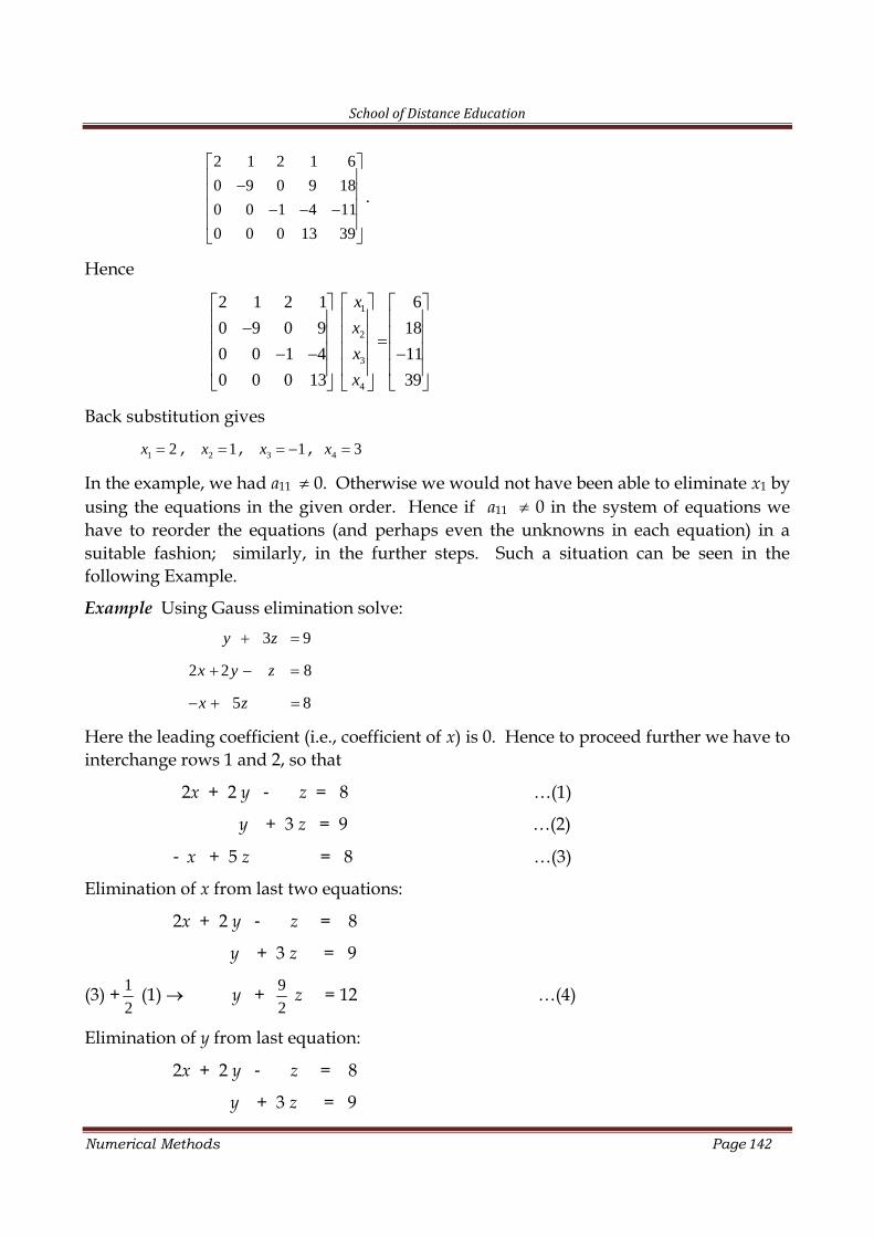
School of Distance Education
Numerical Methods Page 142
2 1 2 1 6
0 9 0 9 18
0 0 1 4 11
0 0 0 13 39
.
Hence
1
2
3
4
2 1 2 1 6
0 9 0 9 18
0 0 1 4 11
0 0 0 13 39
x
x
x
x
Back substitution gives
1 2x , 2 1x , 3 1 x , 4 3x
In the example, we had a11 0. Otherwise we would not have been able to eliminate x1 byusing the equations in the given order. Hence if a11 0 in the system of equations wehave to reorder the equations (and perhaps even the unknowns in each equation) in asuitable fashion; similarly, in the further steps. Such a situation can be seen in thefollowing Example.
Example Using Gauss elimination solve:3 9
2 2 8
5 8
y z
x y z
x z
Here the leading coefficient (i.e., coefficient of x) is 0. Hence to proceed further we have tointerchange rows 1 and 2, so that
2x + 2 y z = 8 …(1)
y + 3 z = 9 …(2)
x + 5 z = 8 …(3)
Elimination of x from last two equations:
2x + 2 y z = 8
y + 3 z = 9
(3) +2
1 (1) y +2
9 z = 12 …(4)
Elimination of y from last equation:
2x + 2 y z = 8
y + 3 z = 9
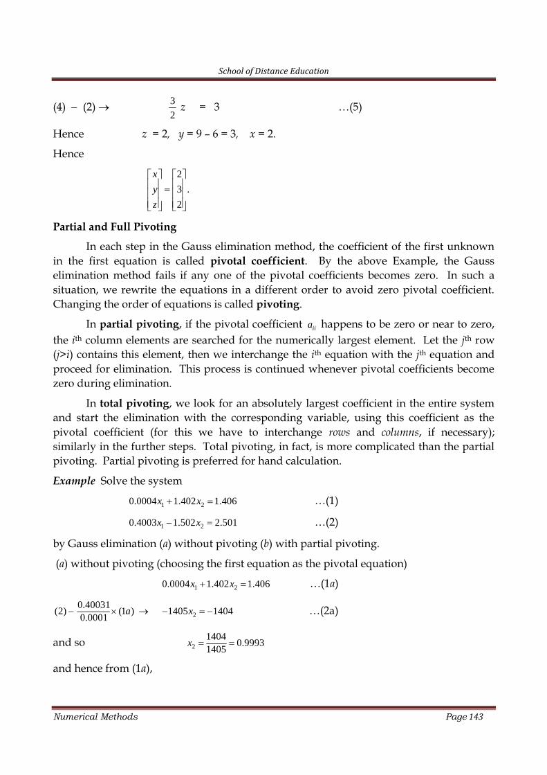
School of Distance Education
Numerical Methods Page 143
(4) (2)2
3 z = 3 …(5)
Hence z = 2, y = 9 – 6 = 3, x = 2.
Hence
2
3 .
2
x
y
z
Partial and Full Pivoting
In each step in the Gauss elimination method, the coefficient of the first unknownin the first equation is called pivotal coefficient. By the above Example, the Gausselimination method fails if any one of the pivotal coefficients becomes zero. In such asituation, we rewrite the equations in a different order to avoid zero pivotal coefficient.Changing the order of equations is called pivoting.
In partial pivoting, if the pivotal coefficient iia happens to be zero or near to zero,the ith column elements are searched for the numerically largest element. Let the jth row(j>i) contains this element, then we interchange the ith equation with the jth equation andproceed for elimination. This process is continued whenever pivotal coefficients becomezero during elimination.
In total pivoting, we look for an absolutely largest coefficient in the entire systemand start the elimination with the corresponding variable, using this coefficient as thepivotal coefficient (for this we have to interchange rows and columns, if necessary);similarly in the further steps. Total pivoting, in fact, is more complicated than the partialpivoting. Partial pivoting is preferred for hand calculation.
Example Solve the system
1 20.0004 1.402 1.406 x x …(1)
1 20.4003 1.502 2.501 x x …(2)
by Gauss elimination (a) without pivoting (b) with partial pivoting.
(a) without pivoting (choosing the first equation as the pivotal equation)
1 20.0004 1.402 1.406 x x …(1a)
0.40031(2) (1 )
0.0001 a 21405 1404 x …(2a)
and so 21404
0.99931405 x
and hence from (1a),
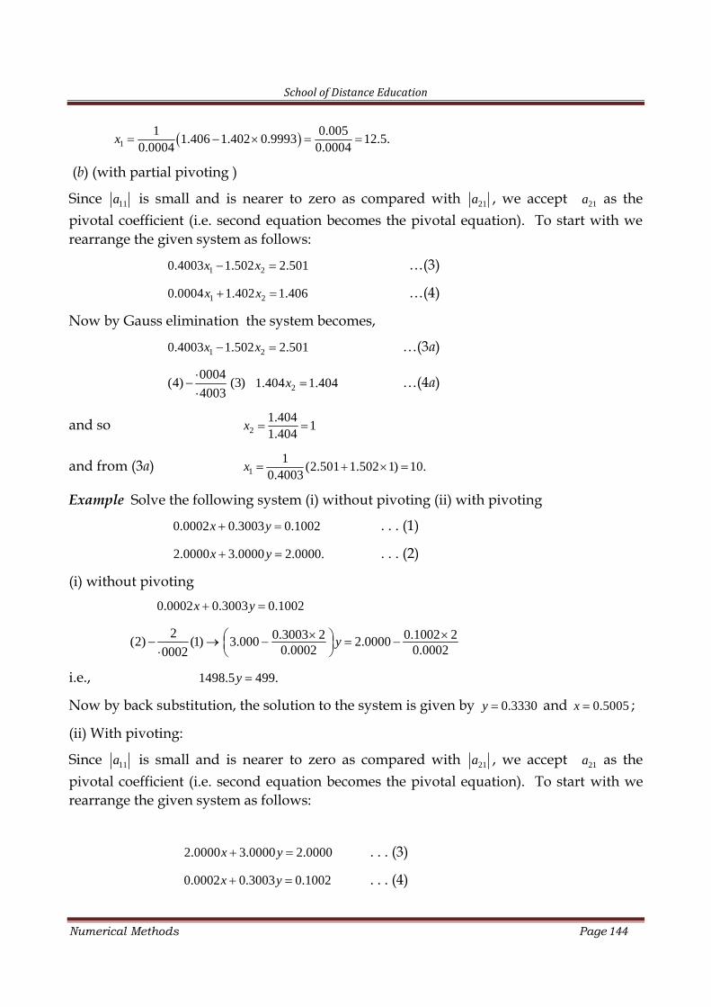
School of Distance Education
Numerical Methods Page 144
11 0.005
1.406 1.402 0.9993 12.5.0.0004 0.0004 x
(b) (with partial pivoting )
Since 11a is small and is nearer to zero as compared with 21a , we accept 21a as thepivotal coefficient (i.e. second equation becomes the pivotal equation). To start with werearrange the given system as follows:
1 20.4003 1.502 2.501 x x …(3)
1 20.0004 1.402 1.406 x x …(4)
Now by Gauss elimination the system becomes,
1 20.4003 1.502 2.501 x x …(3a)
0004(4) (3)
4003
21.404 1.404x …(4a)
and so 21.404
11.404 x
and from (3a) 11
(2.501 1.502 1) 10.0.4003 x
Example Solve the following system (i) without pivoting (ii) with pivoting
0.0002 0.3003 0.1002x y . . . (1)
2.0000 3.0000 2.0000.x y . . . (2)
(i) without pivoting0.0002 0.3003 0.1002x y
2(2) (1)
0002
0.3003 2 0.1002 23.000 2.00000.0002 0.0002
y
i.e., 1498.5 499.y
Now by back substitution, the solution to the system is given by 0.3330y and 0.5005x ;
(ii) With pivoting:
Since 11a is small and is nearer to zero as compared with 21a , we accept 21a as thepivotal coefficient (i.e. second equation becomes the pivotal equation). To start with werearrange the given system as follows:
2.0000 3.0000 2.0000x y . . . (3)
0.0002 0.3003 0.1002x y . . . (4)
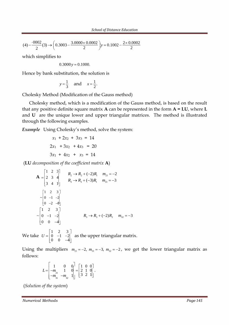
School of Distance Education
Numerical Methods Page 145
0002(4) (3)
2
3.0000 0.0002 2 0.00020.3003 0.1002
2 2
y
which simplifies to0.3000 0.1000.y
Hence by bank substitution, the solution is
13
y and 1 .2
x
Cholesky Method (Modification of the Gauss method)
Cholesky method, which is a modification of the Gauss method, is based on the resultthat any positive definite square matrix A can be represented in the form A = LU, where Land U are the unique lower and upper triangular matrices. The method is illustratedthrough the following examples.
Example Using Cholesky’s method, solve the system:
x1 + 2x2 + 3x3 = 14
2x1 + 3x2 + 4x3 = 20
3x1 + 4x2 + x3 = 14
(LU decomposition of the coefficient matrix A)
A1 2 3
2 3 4
3 4 1
2 2 1 21
3 3 1 31
( 2) 2
( 3) 3
R R R m
R R R m
2
1 2 3
~ 0 1
0 0 4
3 3 2 32( 2) 3 R R R m
We take1 2 30 1 20 0 4
U
as the upper triangular matrix.
Using the multipliers 21 31 322, 3, 2 m m m , we get the lower triangular matrix asfollows:
21
31 32
1 0 0 1 0 01 0 2 1 0
3 2 11L m
m m
.
(Solution of the system)
2
1 2 3
~ 0 1
0 2 8
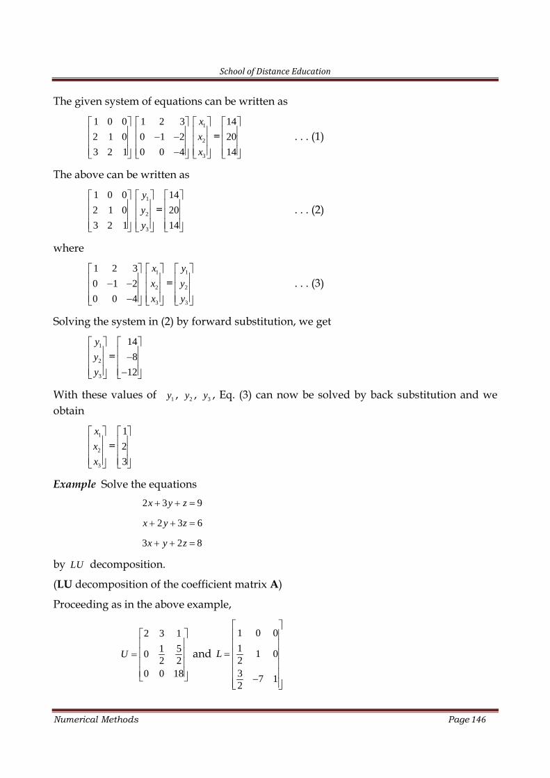
School of Distance Education
Numerical Methods Page 146
The given system of equations can be written as
1 0 0
2 1 0
3 2 1
1 2 3
0 1 2
0 0 4
1
2
3
x
x
x
=14
20
14
. . . (1)
The above can be written as
1 0 0
2 1 0
3 2 1
1
2
3
y
y
y
=14
20
14
. . . (2)
where
1 2 3
0 1 2
0 0 4
1
2
3
x
x
x
=1
2
3
y
y
y
. . . (3)
Solving the system in (2) by forward substitution, we get
1
2
3
y
y
y
=14
8
12
With these values of 1y , 2y , 3y , Eq. (3) can now be solved by back substitution and weobtain
1
2
3
x
x
x
=1
2
3
Example Solve the equations2 3 9x y z
2 3 6x y z
3 2 8x y z
by LU decomposition.
(LU decomposition of the coefficient matrix A)
Proceeding as in the above example,
2 3 1
1 502 2
0 0 18
U
and
1 0 0
1 1 023 7 12
L
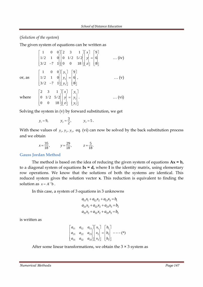
School of Distance Education
Numerical Methods Page 147
(Solution of the system)
The given system of equations can be written as
1 0 0 2 3 1 9
1/ 2 1 0 0 1/ 2 5/ 2 6
3/ 2 7 1 0 0 18 8
x
y
z
… (iv)
or, as1
2
3
1 0 0 9
1/ 2 1 0 6 ,
3/ 2 7 1 8
y
y
y
… (v)
where1
2
3
2 3 1
0 1/ 2 5/ 2 .
0 0 18
x y
y y
z y
… (vi)
Solving the system in (v) by forward substitution, we get
1 9,y 23 ,2
y 3 5y .
With these values of 1 2 3, , ,y y y eq. (vi) can now be solved by the back substitution processand we obtain
35 ,18
x 29 ,18
y 5 .18
z
Gauss Jordan Method
The method is based on the idea of reducing the given system of equations Ax = b,to a diagonal system of equations Ix = d, where I is the identity matrix, using elementaryrow operations. We know that the solutions of both the systems are identical. Thisreduced system gives the solution vector x. This reduction is equivalent to finding thesolution as 1x A b .
In this case, a system of 3 equations in 3 unknowns
11 1 12 2 13 3 1
21 2 22 2 23 3 2
31 2 32 2 33 3 3
a x a x a x b
a x a x a x b
a x a x a x b
is written as
11 12 13 1 1
21 22 23 2 2
31 32 33 3 3
(*)
a a a x b
a a a x b
a a a x b
After some linear transformations, we obtain the 3 × 3 system as
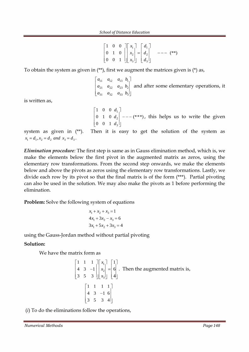
School of Distance Education
Numerical Methods Page 148
1 1
2 2
3 3
1 0 0
0 1 0 (**)
0 0 1
x d
x d
x d
To obtain the system as given in (**), first we augment the matrices given is (*) as,
11 12 13 1
21 22 23 2
31 32 33 3
a a a b
a a a b
a a a b
and after some elementary operations, it
is written as,
1
2
3
1 0 0
0 1 0 (***)
0 0 1
d
d
d
, this helps us to write the given
system as given in (**). Then it is easy to get the solution of the system as1 1 2 2 3 3,x d x d and x d .
Elimination procedure: The first step is same as in Gauss elimination method, which is, wemake the elements below the first pivot in the augmented matrix as zeros, using theelementary row transformations. From the second step onwards, we make the elementsbelow and above the pivots as zeros using the elementary row transformations. Lastly, wedivide each row by its pivot so that the final matrix is of the form (***). Partial pivotingcan also be used in the solution. We may also make the pivots as 1 before performing theelimination.
Problem: Solve the following system of equations
1 2 3
1 2 3
1 2 3
1
4 3 6
3 5 3 4
x x x
x x x
x x x
using the Gauss-Jordan method without partial pivoting
Solution:
We have the matrix form as
1
2
3
1 1 1 1
4 3 1 6
3 5 3 4
x
x
x
. Then the augmented matrix is,
1 1 1 1
4 3 1 6
3 5 3 4
(i) To do the eliminations follow the operations,
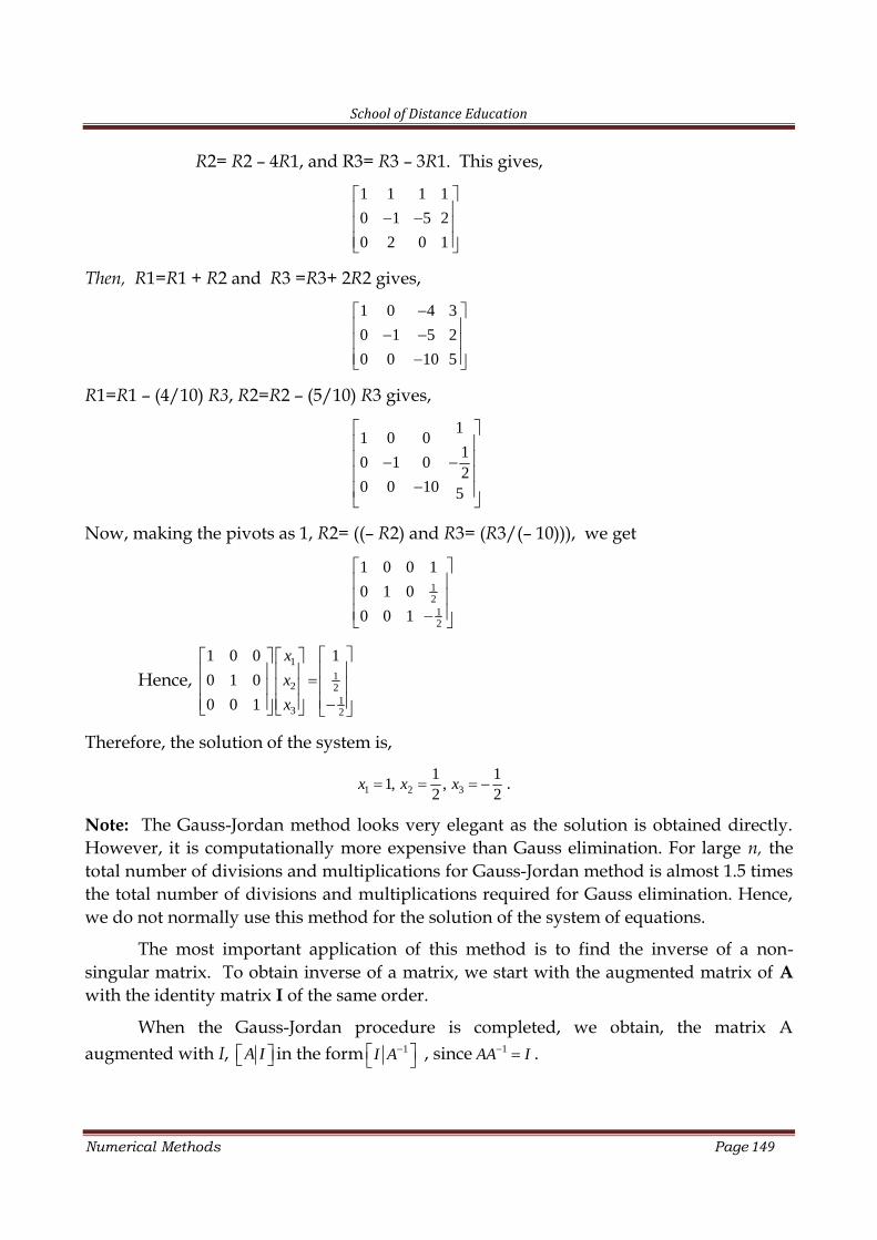
School of Distance Education
Numerical Methods Page 149
R2= R2 – 4R1, and R3= R3 – 3R1. This gives,
1 1 1 1
0 1 5 2
0 2 0 1
Then, R1=R1 + R2 and R3 =R3+ 2R2 gives,
1 0 4 3
0 1 5 2
0 0 10 5
R1=R1 – (4/10) R3, R2=R2 – (5/10) R3 gives,
11 0 0
10 1 0
20 0 10 5
Now, making the pivots as 1, R2= ((– R2) and R3= (R3/(– 10))), we get
1212
1 0 0 1
0 1 0
0 0 1
Hence,1
12 2
13 2
1 0 0 1
0 1 0
0 0 1
x
x
x
Therefore, the solution of the system is,
1 2 31 1
1, ,2 2
x x x .
Note: The Gauss-Jordan method looks very elegant as the solution is obtained directly.However, it is computationally more expensive than Gauss elimination. For large n, thetotal number of divisions and multiplications for Gauss-Jordan method is almost 1.5 timesthe total number of divisions and multiplications required for Gauss elimination. Hence,we do not normally use this method for the solution of the system of equations.
The most important application of this method is to find the inverse of a non-singular matrix. To obtain inverse of a matrix, we start with the augmented matrix of Awith the identity matrix I of the same order.
When the Gauss-Jordan procedure is completed, we obtain, the matrix Aaugmented with I, A I in the form 1I A , since 1AA I .
School of Distance Education
Numerical Methods Page 150
Example Using Gauss Jordan method solve the system of equations:
x + 2y + z = 8 … (1)
2x + 3y + 4z = 20 … (2)
4x + 3y + 2z = 16 … (3)
[Elimination of x from Eqs. (2) and (3), using (1)]
x + 2y + z = 8 … (1a)
y + 2z = 4 … (2a)
5y 2z = 16 … (3a)
[Elimination of y from (1a) and (3a), using (2a)]
x + 5z = 16 … (1b)
y + 2z = 4 … (2b)
12z = 36 … (3b)
[Elimination of z from (1b) and (2b), using (3b)]
x = 1 … (1c)
y = 2 … (2c)
12z = 36 … (3c)
Hence, x = 1, y = 2, z = 3.
Assignments
1. Apply Gauss elimination method to solve the equations:
2 3 5
4 4 3 3
2 3 1
x y z
x y z
x y z
2. Apply Gauss elimination method to solve the equations:
1 2 3
1 2 3
1 2 3
3 6 16
2 4 3 13
3 2 9
x x x
x x x
x x x
3. Apply Gauss elimination method to solve the equations:10 2 9
2 20 2 44
2 3 10 22
x y z
x y z
x y z

School of Distance Education
Numerical Methods Page 151
4. Apply Gauss elimination method to solve the equations:10
2 2 17
3 2 17
x y z
x y z
x y z
5. Solve the system, using Gauss elimination method:
1 2 3 4
1 2 3 4
1 2 3 4
1 2 3 4
5 4
7 12
6 5
4 6
x x x x
x x x x
x x x x
x x x x
6. Apply Gauss elimination method to solve the equations:4 5
6 12
3 4
x y z
x y z
x y z
7. Solve the following system, using Cholesky method10 12
2 10 13
2 2 10 14
x y z
x y z
x y z
8. Solve the following system, using Cholesky method
2 3 5
4 4 3 3
2 3 1
x y z
x y z
x y z
9. Solve the following system, using Cholesky method
2 3 9
2 3 6
3 2 8
x y z
x y z
x y z
10. Solve the following using Cholesky method:
3 1 1 41 2 2 3 .2 1 3 4
xyz
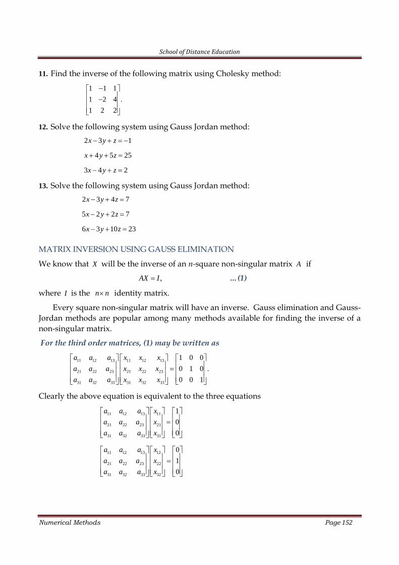
School of Distance Education
Numerical Methods Page 152
11. Find the inverse of the following matrix using Cholesky method:
1 1 1
1 2 4 .
1 2 2
12. Solve the following system using Gauss Jordan method:2 3 1
4 5 25
3 4 2
x y z
x y z
x y z
13. Solve the following system using Gauss Jordan method:2 3 4 7
5 2 2 7
6 3 10 23
x y z
x y z
x y z
MATRIX INVERSION USING GAUSS ELIMINATION
We know that X will be the inverse of an n-square non-singular matrix A if
,AX I …(1)
where I is the n n identity matrix.
Every square non-singular matrix will have an inverse. Gauss elimination and Gauss-Jordan methods are popular among many methods available for finding the inverse of anon-singular matrix.
For the third order matrices, (1) may be written as
11 12 13 11 12 13
21 22 23 21 22 23
31 32 33 31 32 33
1 0 0
0 1 0 .
0 0 1
a a a x x x
a a a x x x
a a a x x x
Clearly the above equation is equivalent to the three equations
11 12 13 11
21 22 23 21
31 32 33 31
1
0
0
a a a x
a a a x
a a a x
11 12 13 12
21 22 23 22
31 32 33 32
0
1
0
a a a x
a a a x
a a a x
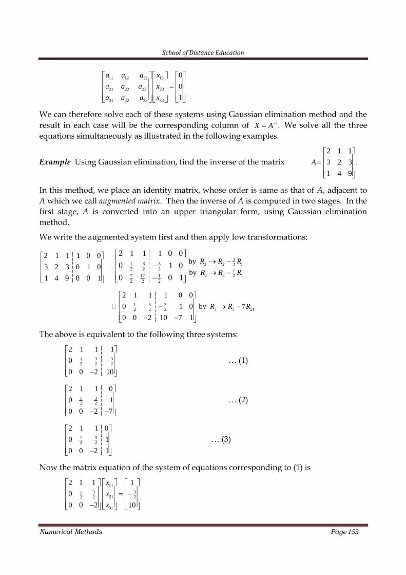
School of Distance Education
Numerical Methods Page 153
11 12 13 13
21 22 23 23
31 32 33 33
0
0
1
a a a x
a a a x
a a a x
We can therefore solve each of these systems using Gaussian elimination method and theresult in each case will be the corresponding column of 1.X A We solve all the threeequations simultaneously as illustrated in the following examples.
Example Using Gaussian elimination, find the inverse of the matrix2 1 1
3 2 3 .
1 4 9
A
In this method, we place an identity matrix, whose order is same as that of A, adjacent toA which we call augmented matrix. Then the inverse of A is computed in two stages. In thefirst stage, A is converted into an upper triangular form, using Gaussian eliminationmethod.
We write the augmented system first and then apply low transformations:
2 1 1 1 0 0
3 2 3 0 1 0
1 4 9 0 0 1
3 31
2 2 2
7 17 12 2 2
2 1 1 1 0 0
0 1 0
0 0 1
32 2 12
13 3 12
by
by
R R R
R R R
3 312 2 2
2 1 1 1 0 0
0 1 0
0 0 2 10 7 1
3 3 21by 7R R R
The above is equivalent to the following three systems:
3 312 2 2
2 1 1 1
0
0 0 2 10
… (1)
312 2
2 1 1 0
0 1
0 0 2 7
… (2)
312 2
2 1 1 0
0 1
0 0 2 1
… (3)
Now the matrix equation of the system of equations corresponding to (1) is
11
3 31212 2 2
31
2 1 1 1
0
0 0 2 10
x
x
x
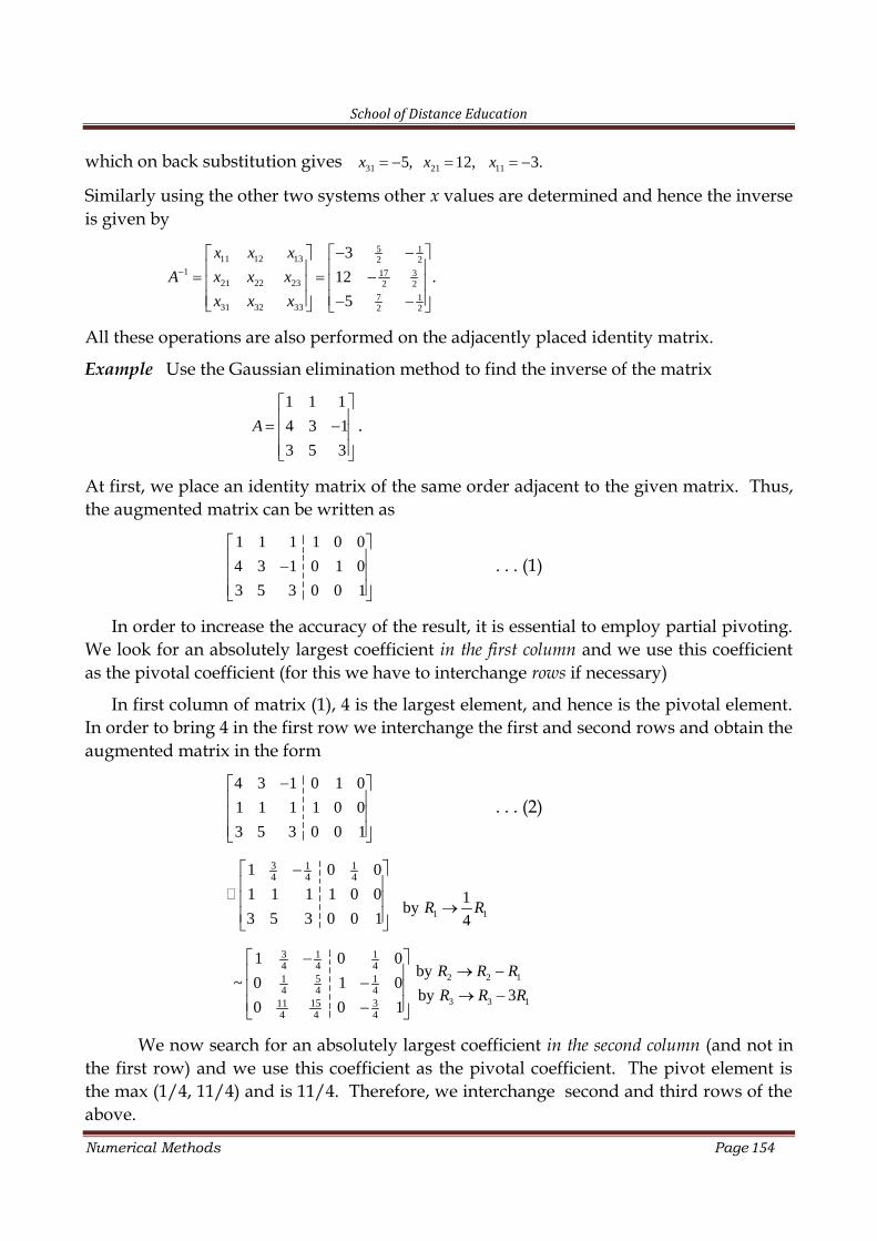
School of Distance Education
Numerical Methods Page 154
which on back substitution gives 31 21 115, 12, 3. x x x
Similarly using the other two systems other x values are determined and hence the inverseis given by
5 111 12 13 2 2
1 17 321 22 23 2 2
7 131 32 33 2 2
3
12 .
5
x x x
A x x x
x x x
All these operations are also performed on the adjacently placed identity matrix.
Example Use the Gaussian elimination method to find the inverse of the matrix
1 1 1
4 3 1
3 5 3
A .
At first, we place an identity matrix of the same order adjacent to the given matrix. Thus,the augmented matrix can be written as
1 1 1 1 0 0
4 3 1 0 1 0
3 5 3 0 0 1
. . . (1)
In order to increase the accuracy of the result, it is essential to employ partial pivoting.We look for an absolutely largest coefficient in the first column and we use this coefficientas the pivotal coefficient (for this we have to interchange rows if necessary)
In first column of matrix (1), 4 is the largest element, and hence is the pivotal element.In order to bring 4 in the first row we interchange the first and second rows and obtain theaugmented matrix in the form
4 3 1 0 1 0
1 1 1 1 0 0
3 5 3 0 0 1
. . . (2)
3 1 14 4 41 0 0
1 1 1 1 0 0
3 5 3 0 0 1
1 1
1by
4R R
3 1 14 4 4
51 14 4 4
15 3114 4 4
1 0 0
~ 0 1 0
0 0 1
2 2 1
3 3 1
by
by 3
R R R
R R R
We now search for an absolutely largest coefficient in the second column (and not inthe first row) and we use this coefficient as the pivotal coefficient. The pivot element isthe max (1/4, 11/4) and is 11/4. Therefore, we interchange second and third rows of theabove.
School of Distance Education
Numerical Methods Page 155
3 1 14 4 4
15 3114 4 4
51 14 4 4
1 0 0
0 0 1
0 1 0
Now, divide R2 by the pivot element a22 = 11/4, and obtain3 1 14 4 4
15 3 411 11 1151 1
4 4 4
1 0 0
0 1 0
0 1 0
In order to make the entries below 1 in the second column we perform
R3 R3 (1/4)R1 in the above matrix and obtain3 1 14 4 4
15 3 411 11 1110 2 111 11 11
1 0 0
0 1 0
0 0 1
This is equivalent to the following three matrices3 14 4
15111011
1 0
0 1 0
0 0 1
;
3 1 14 4 4
15 310 1110 211 11
1
0 1
0 0
;
3 14 4
15 411 1110 111 11
1 0
0 1
0 0
Thus we have
11 12 131
21 22 23
31 32 33
7 1 25 5 53 1
02 2
11 1 110 5 10
x x x
A x x x
x x x
Matrix Inversion using Gauss-Jordan method
This method is similar to Gaussian elimination method for matrix inversion, starting withthe augmented matrix [ ]AI and reducing A to the identity matrix using elementary rowtransformations. The method is illustrated in the following example.
Example Find the inverse of the following matrix A by Gauss-Jordan method.
1 1 1
4 3 1 .
3 5 3
A
The augmented matrix is given by
School of Distance Education
Numerical Methods Page 156
1 1 1 1 0 0
4 3 1 0 1 0
3 5 3 0 0 1
1 1 1 1 0 0
~ 0 1 5 4 1 0
0 2 0 3 0 1
2 2 1
3 3 1
by 4
by 3
R R R
R R R
1 1 1 1 0 0
~ 0 1 5 4 1 0
0 2 0 3 0 1
2 2by R R
1 0 4 3 1 0
~ 0 1 5 4 1 0
0 0 10 11 2 1
1 1 2
3 3 2
by
by 2
R R R
R R R
1 0 4 3 1 0
~ 0 1 5 4 1 0
0 0 1 11/10 1/ 5 1/10
3 3
1by
10R R
1 0 0 7 / 5 1/ 5 2 / 5
~ 0 1 0 3/ 2 0 1/ 2
0 0 1 11/10 1/ 5 1/10
1 1 3
2 2 1
by 4
by 5
R R R
R R R
Thus we have
1
7 1 25 5 53 1
0 .2 2
11 1 110 5 10
A
Triangulation Method (LU Decomposition Method):
In linear algebra, LU decomposition (also called LU factorization) factorizes amatrix as the product of a lower triangular matrix and an upper triangular matrix
Let A be a non-singular square matrix. LU decomposition is a decomposition of theform
A=LU
where L is a lower triangular matrix and U is an upper triangular matrix. This means thatL has only zeros above the diagonal and U has only zeros below the diagonal. Forexample, for a 3-by-3 matrix A, its LU decomposition looks like this:
School of Distance Education
Numerical Methods Page 157
11 12 13 11 12 13
21 22 23 21 22 23
31 32 33 31 32 33
1 0 0
1 0 0
1 0 0
a a a u u u
a a a l u u
a a a l l u
Consider a system of linear equations,
11 1 12 2 13 3 1
21 1 22 2 23 3 2
31 1 32 2 33 3 3
a x a x a x b
a x a x a x b
a x a x a x b
This can be written in the form,
Ax=b,
where11 12 13
21 22 23
31 32 33
a a a
A a a a
a a a
,12..
xx
xn
x
and12..
bb
bm
b
To solve the system of equations by LU decomposition, first we decompose A as LU,where,
11 12 13
21 22 23
31 32 33
1 0 0
1 0 0
1 0 0
u u u
L l and U u u
l l u
This gives,
LUx = b.
Let Ux=y. This implies, Ly=b.
That is,
1 1
21 2 2
31 32 3 3
1 0 0
1 0
1
y b
l y b
l l y b
Thus,
1 1
21 1 2 2
31 1 32 2 3 3
y b
l y y b
l y l y y b
School of Distance Education
Numerical Methods Page 158
This gives the y values by forward substitution, which means, substitute the valueof 1y given by the first equation in the second and solve 2y , then use these values of
1 2y and y in the third and solve 3y .
Then the system of equations
11 12 13 1 1
22 23 2 2
33 3 3
; 0
0 0
u u u x y
Ux y that is u u x y
u x y
gives the required values of 1 2 3,x x and x as the solution of the original system of linearequations by backward substitution.
To decompose a matrix11 12 13
21 22 23
31 32 33
a a a
A a a a
a a a
, in the form
11 12 13 11 12 13
21 22 23 21 22 23
31 32 33 31 32 33
1 0 0
1 0 0
1 0 0
a a a u u u
a a a l u u
a a a l l u
, we proceed as follows.
On multiplying11 12 13
21 22 23
31 32 33
1 0 0
1 0 0
1 0 0
u u u
l and u u
l l u
, we get,
11 12 13
21 11 21 12 22 21 13 23
31 11 31 12 32 22 31 13 32 23 33
u u u
l u l u u l u u
l u l u l u l u l u u
Equating it with the corresponding terms of A, we get,
11 11 12 12 13 13
312121 11 21 21 31 11 31 31
11 11
21 12 22 22 22 22 21 12
21 13 23 23 23 23 21 13
31 12 32 22 32 31 13 32 23 33 33 32 33
; ;
;
;
;
,
,
u a u a u a
aal u a l l u a l
u u
l u u a u a l u
l u u a u a l u
simililarly
l u l u a l u l u u a gives l and u
.
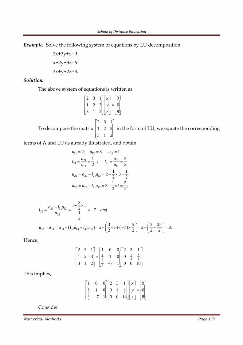
School of Distance Education
Numerical Methods Page 159
Example: Solve the following system of equations by LU decomposition.
2x+3y+z=9
x+2y+3z=6
3x+y+2z=8.
Solution:
The above system of equations is written as,
2 3 1 9
1 2 3 6
3 1 2 8
x
y
z
To decompose the matrix2 3 1
1 2 3
3 1 2
in the form of LU, we equate the corresponding
terms of A and LU as already illustrated, and obtain
11 12 13
312121 31
11 11
22 22 21 12
23 23 21 13
2; 3; 1
1 3;
2 2
1 12 3 ;
2 21 5
3 1 ;2 2
u u u
aal l
u u
u a l u
u a l u
32 31 1232
22
33 33 33 31 13 32 23
31 3
2 712
3 5 3 352 1 7 2 18
2 2 2 2
a l ul and
u
u u a l u l u
Hence,
51 12 2 232
2 3 1 1 0 0 2 3 1
1 2 3 1 0 0
3 1 2 7 1 0 0 18
This implies,
51 12 2 232
1 0 0 2 3 1 9
1 0 0 6
7 1 0 0 18 8
x
y
z
Consider
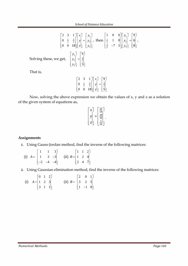
School of Distance Education
Numerical Methods Page 160
151
22 2
3
2 3 1
0
0 0 18
x y
y y
z y
, then1
122
332
1 0 0 9
1 0 6
7 1 8
y
y
y
,
Solving these, we get,1
32 2
3
9
5
y
y
y
That is,
5 312 2 2
2 3 1 9
0
0 0 18 5
x
y
z
Now, solving the above expression we obtain the values of x, y and z as a solutionof the given system of equations as,
351829185
18
x
y
z
.
Assignments
1. Using Gauss-Jordan method, find the inverse of the following matrices:
(i)1 1 3
1 3 3
2 4 4
A
(ii)1 1 2
1 2 4
2 4 7
B
2. Using Gaussian elimination method, find the inverse of the following matrices:
(i)0 1 2
1 2 3
3 1 1
A
(ii)2 0 1
3 2 5
1 1 0
B
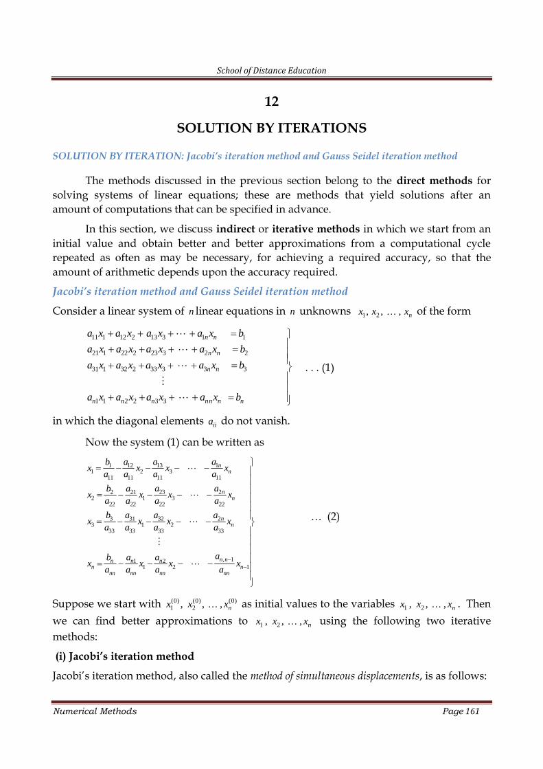
School of Distance Education
Numerical Methods Page 161
12
SOLUTION BY ITERATIONS
SOLUTION BY ITERATION: Jacobi’s iteration method and Gauss Seidel iteration method
The methods discussed in the previous section belong to the direct methods forsolving systems of linear equations; these are methods that yield solutions after anamount of computations that can be specified in advance.
In this section, we discuss indirect or iterative methods in which we start from aninitial value and obtain better and better approximations from a computational cyclerepeated as often as may be necessary, for achieving a required accuracy, so that theamount of arithmetic depends upon the accuracy required.
Jacobi’s iteration method and Gauss Seidel iteration method
Consider a linear system of n linear equations in n unknowns 1 2, , , nx x x of the form
11 1 12 2 13 3 1 1
21 1 22 2 23 3 2 2
31 1 32 2 33 3 3 3
1 1 2 2 3 3
n n
n n
n n
n n n nn n n
a x a x a x a x b
a x a x a x a x b
a x a x a x a x b
a x a x a x a x b
. . . (1)
in which the diagonal elements iia do not vanish.
Now the system (1) can be written as
13 11 121 2 3
11 11 11 11
23 22 212 1 3
22 22 22 22
3 31 32 23 1 2
33 33 33 33
, 11 21 2 1
nn
nn
nn
n nn n nn n
nn nn nn nn
a ab ax x x x
a a a a
a ab ax x x x
a a a a
b a a ax x x x
a a a a
ab a ax x x x
a a a a
… (2)
Suppose we start with (0) (0) (0)1 2, , , nx x x as initial values to the variables 1 2, , , nx x x . Then
we can find better approximations to 1 2, , , nx x x using the following two iterativemethods:
(i) Jacobi’s iteration method
Jacobi’s iteration method, also called the method of simultaneous displacements, is as follows:
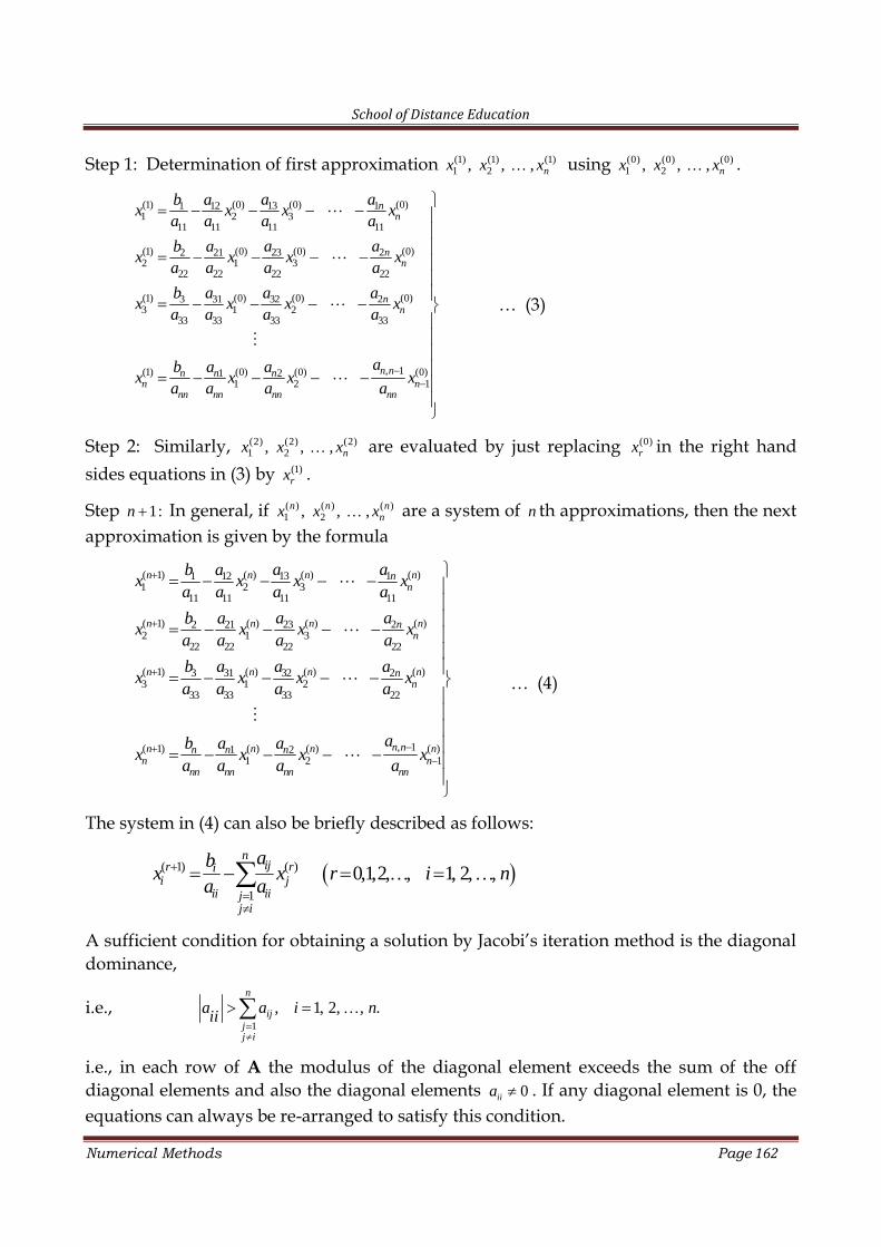
School of Distance Education
Numerical Methods Page 162
Step 1: Determination of first approximation (1) (1) (1)1 2, , , nx x x using (0) (0) (0)
1 2, , , nx x x .
(1) (0) (0) (0)13 11 121 2 3
11 11 11 11
(1) (0) (0) (0)23 22 212 1 3
22 22 22 22
(1) (0) (0) (0)3 31 32 23 1 2
33 33 33 33
, 1(1) (0) (0) (1 21 2 1
nn
nn
nn
n nn n nn n
nn nn nn nn
a ab ax x x x
a a a a
a ab ax x x x
a a a a
b a a ax x x x
a a a a
ab a ax x x x
a a a a0)
… (3)
Step 2: Similarly, (2) (2) (2)1 2, , , nx x x are evaluated by just replacing (0)
rx in the right handsides equations in (3) by (1)
rx .
Step 1:n In general, if ( ) ( ) ( )1 2, , ,n n n
nx x x are a system of n th approximations, then the nextapproximation is given by the formula
( 1) ( ) ( ) ( )13 11 121 2 3
11 11 11 11
( 1) ( ) ( ) ( )23 22 212 1 3
22 22 22 22
( 1) ( ) ( ) ( )3 31 32 23 1 2
33 33 33 22
, 1( 1) ( ) ( )1 21 2
n n n nnn
n n n nnn
n n n nnn
n nn n nn n nn
nn nn nn
a ab ax x x x
a a a a
a ab ax x x x
a a a a
b a a ax x x x
a a a a
ab a ax x x
a a a( )
1
nn
nn
xa
… (4)
The system in (4) can also be briefly described as follows:
( 1) ( )
1
0,1,2, , 1, 2, ,
n
ijr rii j
ii iijj i
abx x r i n
a a
A sufficient condition for obtaining a solution by Jacobi’s iteration method is the diagonaldominance,
i.e.,1
, 1, 2, , .
n
ijjj i
a a i nii
i.e., in each row of A the modulus of the diagonal element exceeds the sum of the offdiagonal elements and also the diagonal elements 0iia . If any diagonal element is 0, theequations can always be re-arranged to satisfy this condition.
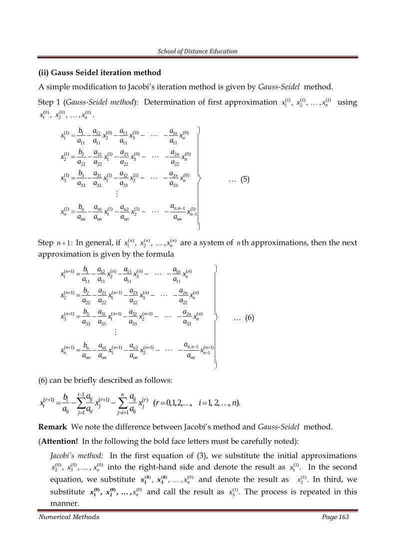
School of Distance Education
Numerical Methods Page 163
(ii) Gauss Seidel iteration method
A simple modification to Jacobi’s iteration method is given by Gauss-Seidel method.
Step 1 (Gauss-Seidel method): Determination of first approximation (1) (1) (1)1 2, , , nx x x using
(0) (0) (0)1 2, , , nx x x .
(1) (0) (0) (0)13 11 121 2 3
11 11 11 11
(1) (1) (0) (0)23 22 212 1 3
22 22 22 22
(1) (1) (1) (0)3 31 32 23 1 2
33 33 33 33
, 1(1) (1) (1) (1 21 2 1
nn
nn
nn
n nn n nn n
nn nn nn nn
a ab ax x x x
a a a a
a ab ax x x x
a a a a
b a a ax x x x
a a a a
ab a ax x x x
a a a a1)
… (5)
Step 1:n In general, if ( ) ( ) ( )1 2, , ,n n n
nx x x are a system of n th approximations, then the nextapproximation is given by the formula
( 1) ( ) ( ) ( )13 11 121 2 3
11 11 11 11
( 1) ( 1) ( ) ( )23 22 212 1 3
22 22 22 22
( 1) ( 1) ( 1) ( )3 31 32 23 1 2
33 33 33 33
( 1) ( 1) ( 11 21 2
n n n nnn
n n n nnn
n n n nnn
n n nn n nn
nn nn nn
a ab ax x x x
a a a a
a ab ax x x x
a a a a
b a a ax x x x
a a a a
b a ax x x
a a a, 1) ( 1)
1
n n n
nnn
ax
a
… (6)
(6) can be briefly described as follows:
1( 1) ( 1) ( )
1 1
( 0,1,2, , 1, 2, , ).
i n
ij ijr r rii j j
ii ii iij j i
a abx x x r i n
a a a
Remark We note the difference between Jacobi’s method and Gauss-Seidel method.
(Attention! In the following the bold face letters must be carefully noted):
Jacobi’s method: In the first equation of (3), we substitute the initial approximations(0) (0) (0)2 3, , , nx x x into the right-hand side and denote the result as (1)
1 .x In the secondequation, we substitute ( ) ( ) (0), , , nx0 0
1 3x x and denote the result as (1)2 .x In third, we
substitute (0)nx(0) (0)
1 2, , … ,x x and call the result as (1)3 .x The process is repeated in this
manner.
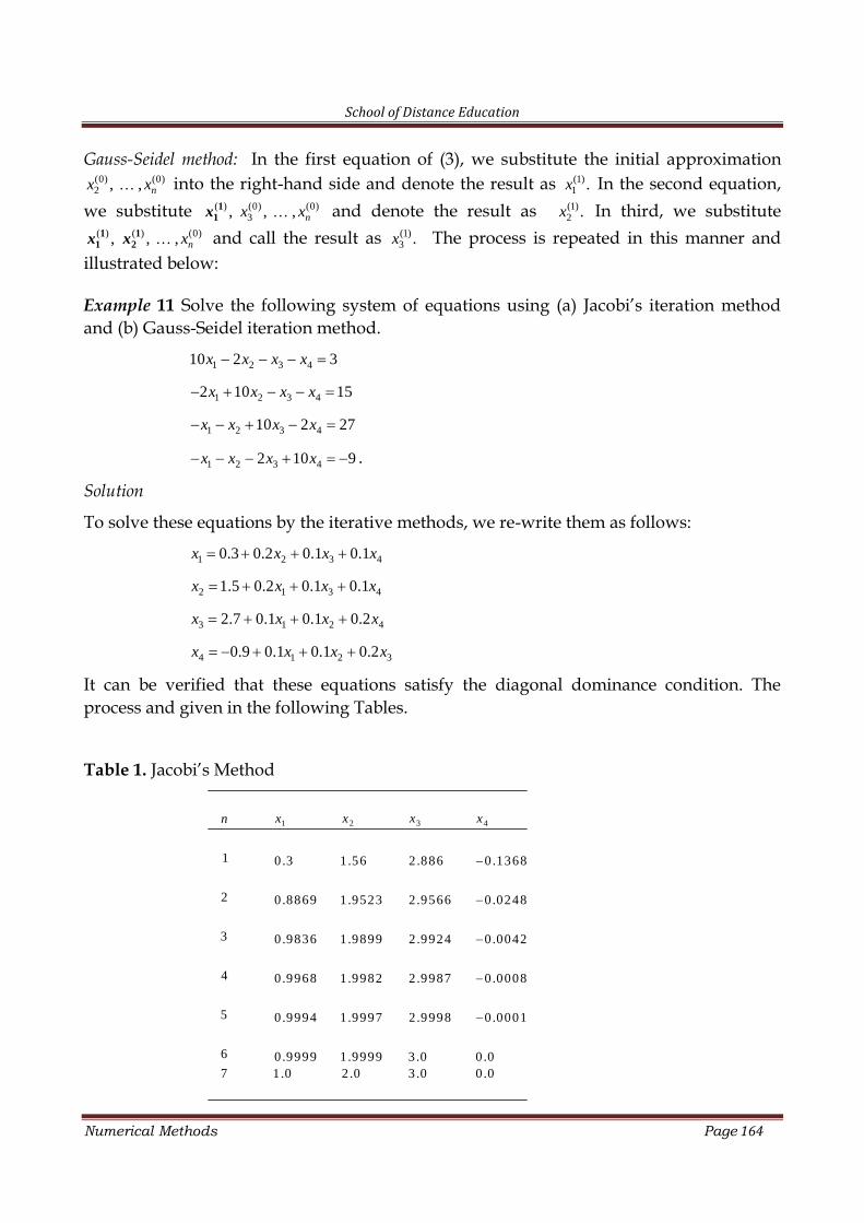
School of Distance Education
Numerical Methods Page 164
Gauss-Seidel method: In the first equation of (3), we substitute the initial approximation(0) (0)2 , , nx x into the right-hand side and denote the result as (1)
1 .x In the second equation,we substitute ( ) (0) (0)
3, , , nx x11x and denote the result as (1)
2 .x In third, we substitute( ) ( ) (0), , , nx1 11 2x x and call the result as (1)
3 .x The process is repeated in this manner andillustrated below:
Example 11 Solve the following system of equations using (a) Jacobi’s iteration methodand (b) Gauss-Seidel iteration method.
1 2 3 410 2 3x x x x
1 2 3 42 10 15x x x x
1 2 3 410 2 27x x x x
1 2 3 42 10 9x x x x .
Solution
To solve these equations by the iterative methods, we re-write them as follows:
1 2 3 40.3 0.2 0.1 0.1x x x x
2 1 3 41.5 0.2 0.1 0.1x x x x
3 1 2 42.7 0.1 0.1 0.2x x x x
4 1 2 30.9 0.1 0.1 0.2x x x x
It can be verified that these equations satisfy the diagonal dominance condition. Theprocess and given in the following Tables.
Table 1. Jacobi’s Method
31 2 4
1 0.3 1.56 2.886 0.1368
2 0.8869 1.9523 2.9566 0.0248
3 0.9836 1.9899 2.9924 0.0042
4 0.9968 1.9982 2.9987 0.0008
5 0.9994 1.9997 2.9998 0.0001
6 0.9999 1.9999 3.0 0.07 1.0 2.0 3.0 0.0
xx x xn
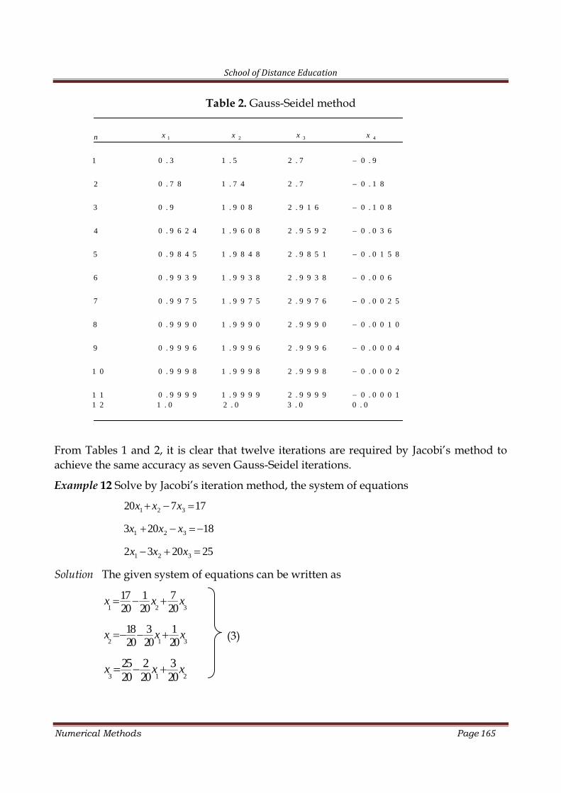
School of Distance Education
Numerical Methods Page 165
Table 2. Gauss-Seidel method
From Tables 1 and 2, it is clear that twelve iterations are required by Jacobi’s method toachieve the same accuracy as seven Gauss-Seidel iterations.
Example 12 Solve by Jacobi’s iteration method, the system of equations
1 2 3
1 2 3
1 2 3
20 7 17
3 20 18
2 3 20 25
x x x
x x x
x x x
Solution The given system of equations can be written as
1 2 3
17 1 720 20 20
x x x
2 1 3
18 3 120 20 20
x x x (3)
3 1 2
25 2 320 20 20
x x x
31 2 4
0 . 3 1 . 5 2 . 7 0 . 91
0 . 7 8 1 . 7 4 2 . 7 0 . 1 82
3 0 . 9 1 . 9 0 8 2 . 9 1 6 0 . 1 0 8
0 . 9 6 2 4 1 . 9 6 0 8 2 . 9 5 9 2 0 . 0 3 64
5 0 . 9 8 4 5 1 . 9 8 4 8 2 . 9 8 5 1 0 . 0 1 5 8
6 0 . 9 9 3 9 1 . 9 9 3 8 2 . 9 9 3 8 0 . 0 0 6
7 0 . 9 9 7 5 1 . 9 9 7 5 2 . 9 9 7 6 0 . 0 0 2 5
8 0 . 9 9 9 0 1 . 9 9 9 0 2 . 9 9 9 0 0 . 0 0 1 0
9 0 . 9 9 9 6 1 . 9 9 9
xx x xn
6 2 . 9 9 9 6 0 . 0 0 0 4
1 0 0 . 9 9 9 8 1 . 9 9 9 8 2 . 9 9 9 8 0 . 0 0 0 2
0 . 9 9 9 9 1 . 9 9 9 9 2 . 9 9 9 9 0 . 0 0 0 11 11 2 1 . 0 2 . 0 3 . 0 0 . 0
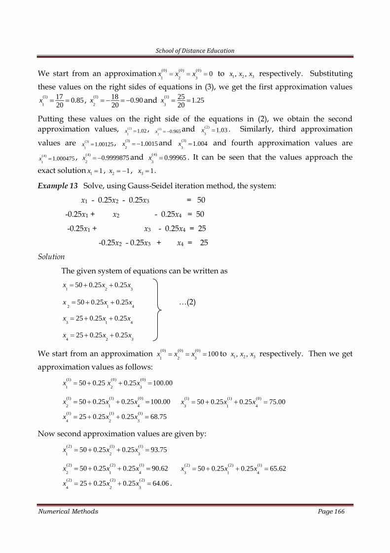
School of Distance Education
Numerical Methods Page 166
We start from an approximation (0) (0) (0)
1 2 30 x x x to 1 2 3, ,x x x respectively. Substituting
these values on the right sides of equations in (3), we get the first approximation values(1)
1
17 0.8520
x , (1)
2
18 0.9020
x and (1)
3
25 1.2520
x
Putting these values on the right side of the equations in (2), we obtain the secondapproximation values, (2)
11.02x , (2)
20.965x and (2)
31.03x . Similarly, third approximation
values are (3)
11.00125x , (3)
21.0015x and (3)
31.004x and fourth approximation values are
(4)
11.000475x , (4)
20.9999875x and (4)
30.99965x . It can be seen that the values approach the
exact solution 1 1x , 2 1x , 3 1x .
Example 13 Solve, using Gauss-Seidel iteration method, the system:
x1 - 0.25x2 - 0.25x3 = 50
-0.25x1 + x2 - 0.25x4 = 50
-0.25x1 + x3 - 0.25x4 = 25
-0.25x2 - 0.25x3 + x4 = 25
Solution
The given system of equations can be written as
1 2 350 0.25 0.25x x x
2 1 450 0.25 0.25x x x …(2)
3 1 425 0.25 0.25x x x
4 2 325 0.25 0.25x x x
We start from an approximation (0) (0) (0)
1 2 3100x x x to 1 2 3, ,x x x respectively. Then we get
approximation values as follows:(1) (0) (0)
1 2 350 0.25 0.25 100.00x x x
(1) (1) (0)
2 1 450 0.25 0.25 100.00x x x (1) (1) (0)
3 1 450 0.25 0.25 75.00x x x
(1) (1) (1)
4 2 325 0.25 0.25 68.75x x x
Now second approximation values are given by:(2) (1) (1)
1 2 350 0.25 0.25 93.75x x x
(2) (2) (1)
2 1 450 0.25 0.25 90.62x x x (2) (2) (1)
3 1 450 0.25 0.25 65.62x x x
(2) (2) (2)
4 2 325 0.25 0.25 64.06x x x .
School of Distance Education
Numerical Methods Page 167
Note that the exact solution to the system is
1 2 3 487.5, 62.5x x x x
Example 14 Using Gauss Siedel iteration solve the following system of equations, in threesteps starting from 1, 1, 1.
10 6x y z
10 6x y z
10 6x y z
Solution 0.6 0.1 0.1x y z
0.6 0.1 0.1
0.6 0.1 0.1
y x z
z x y
Step 1 Using x(0) = y(0) = z(0) = 1, we have
x(1) = 0.6 0.1 y(0) 0.1 z(0) = 0.6 0.1 0.1 = 0.4
y(1) = 0.6 0.1 x(1) 0.1 z(0) = 0.6 0.10.4 0.1 = 0.46
z(1) = 0.6 0.1 x(1) 0.1 y(1) = 0.6 0.10.4 0.10.46 = 0.514
Step 2 Using x(1) = 0.4, y(1)= 0.46, z(1) = 0.514, we have
x(2) = 0.6 0.1 y(1) 0.1 z(1) = 0.6 0.1 0.46 0.10.514 = 0.5026
y(2) = 0.6 0.1 x(2) 0.1 z(1) = 0.6 0.10.5026 0.10.514 = 0.49834
z(2) = 0.6 0.1 x(2) 0.1 y(2)
= 0.6 0.10.5026 0.10.49834 = 0.499906
Step 3 Using x(2) = 0.5026, y(2)= 0.49834, z(2) = 0.499906, we have
x(3) = 0.6 0.1 y(2) 0.1 z(2) = 0.6 0.1 0.49834 0.10.499906= 0.5001754
y(3) = 0.6 0.1 x(3) 0.1 z(2)
= 0.6 0.10.5001754 0.10.499906= 0.49999186
z(3) = 0.6 0.1 x(3) 0.1 y(3)
= 0.6 0.10.5001754 0.10.5001754= 0.49996492
We take x 5, y 5, z 5 as the solution of the given system of equations.
School of Distance Education
Numerical Methods Page 168
Exercises
1. Apply Gauss Seidel iteration method to solve:10 2 9x y z
2 20 2 44x y z
2 3 10 22x y z
2. Apply Gauss Seidel iteration method to solve:1.2 2.1 4.2 9.9x y z
5.3 6.1 4.7 21.6x y z
9.2 8.3 15.2x y z
3. Apply Jacobi’s iteration method to solve:5 10x y z
2 10x y z
5 1x y z
4. Apply Jacobi’s iteration method to solve:5 2 12x y z
4 2 15x y z
2 5 20x y z
Answers
1. 1.013, 1.996, 3.001x y z
2. 2, 3, 4x y z (Approximately)
3. 13.223, 16.766, 2.306x y z
4. 2.556, 1.722, 1.005x y z
5. 1.08, 1.95, 3.16x y z
School of Distance Education
Numerical Methods Page 169
13
EIGEN VALUES
Eigen Values
Definitions Suppose λ be an indeterminate. Consider the n × n matrix
nnji
nnnn
n
n
a
aaa
aaa
aaa
A
][
...
......
...
...
21
22221
11211
. . . (1)
Then the matrix A – λI , where I is the identity matrix of order n, is called thecharacteristic matrix of A and is given by
.
...
...
...
...
21
2
1
2221
1211
nnnn
n
n
aaa
a
a
aa
aa
IA . . . (2)
The determinant A λI of the characteristic matrix of A given in (2) can be found outto be
b0 + b1 λ + b2 λ2 + . . . + bn 1λn 1 + bn λn . . . (3)
where b i are scalars. Now (3) is a non-zero polynomial of degree n in theindeterminate λ. This polynomial is called the characteristic polynomial of A. That isthe characteristic polynomial of the matrix A is given by
A λI . . . . (3)
The equation
A λI = 0 . . . (4)
i.e., the equation
11 12 1
21 22 2
1 2
. . .
. . .0
. . .
. . .
n
n
n n nn
a a a
a a a
a a a
…(4)
is called the characteristic equation of the matrix A.
School of Distance Education
Numerical Methods Page 170
The roots of the characteristic equation (4) are called the characteristic roots or latentroots or eigen values of the matrix A. If is an eigen value, then column vector X suchthat AX X is called an eigen vector associated with the eigen value .
Example Find the eigen values and the corresponding eigen vectors of the matrix
.
342
476
268
A
Solution
The characteristic equation of A is A λI = 0.
i.e., 0
342
476
268
On simplification we get
- λ 3 + 18 λ2 45 λ = 0,
which gives the eigen values λ = 0; λ = 3; λ = 15.
(Determination of eigen vector corresponding to the eigen value 0 )
Let1
2
3
x
X x
x
be the eigen vector corresponding to 0 is obtained by solving 0AX X
i.e., by solving
1 1
2 2
3 3
8 6 2
6 7 4 0
2 4 3
x x
x x
x x
i.e., by solving
.
0
0
0
342
476
268
3
2
1
x
x
x
The corresponding system of linear equations is
1 2 3
1 2 3
1 2 3
8 6 2 0
6 7 4 0
2 4 3 0
x x x
x x x
x x x
1
2
3
Now (1) and (3) can be written as
School of Distance Education
Numerical Methods Page 171
034 321 xxx
and .0342 321 xxx
Now by the method of cross multiplication
234434214133321
xxx
or10105321
xxx .
or221321 xxx
.
Hence 31 2 ,1 2 2
xx xk
where k is arbitrary.
1 2 3, 2 , 2 . x k x k x k . . . (4)
The solution given in (4) also satisfies the equation (2).
eigen vector corresponding to λ = 0 is given by
k
k
k
X
2
2 .
A particular eigen value is (with 1k ) is1
2 .
2
X
(Determination of eigen vector corresponding to the eigen value λ = 3 )
The eigen vector X corresponding to λ = 3 is obtained by solving 3AX X or by solving(A – 3 I) X = 0
i.e., by solving
.
0
0
0
042
446
265
3
2
1
x
x
x
By elementary row transformations, the above matrix equation is equivalent to thematrix equation
.
0
0
0
000
10
101
3
2
1
21
x
x
x
Choosing 3 ,x k arbitrary, we have 1 3 0, x x 12 32 0 x x .
School of Distance Education
Numerical Methods Page 172
Hence 12
k
X k
k
is an eigen vector corresponding to the eigen value λ = 3.
A particular eigen value is (with 2k ) is2
1 .
2
X
(Determination of eigen vector corresponding to the eigen value λ = 15 )
The eigen vector X corresponding to λ = 15 is obtained by solving 15AX X
i.e., by solving (A – 15 I) X = 0
i.e., by solving
.
0
0
0
1242
486
267
3
2
1
x
x
x
Hence
a
a
a
X 2
2
is an eigen vector corresponding to the eigen value λ = 15.
ExampleFind the eigen values and the eigen vector corresponding to the largest eigenvalue of the matrix
.
312
132
226
A
Solution
It can be seen that the eigen values are 2, 2 and 8.
Now we determine the eigen vector corresponding to the largest eigen value 8:
The eigen vector X corresponding to λ = 8 is obtained by solving 8AX X i.e., bysolving [A – 8 I ] X = 0
i.e., by solving
.
0
0
0
8312
1832
2286
3
2
1
x
x
x
School of Distance Education
Numerical Methods Page 173
i.e., by solving
.
0
0
0
512
142
222
3
2
1
x
x
x
The corresponding system of linear equations is
32
1
052
052
0222
321
321
321
xxx
xxx
xxx
Now (1) and (3) can be written as
1 2 3 0 x x x
and .052 321 xxx
Now by the method of cross multiplication
31 2
1 5 1 1 1 2 1 5 1 1 1 2
xx x
or336321 xxx
.
or112321 xxx
.
Hence .112321 k
xxx
.,,2 321 kxkxkx . . . (4)
The solution given in (4) also satisfies the equation (2).
the eigen vector corresponding to λ = 8 is
.
2
k
k
k
X
A particular eigen value is (with 1k ) is2
1 .
1
X
Example Find the eigenvalues and eigenvectors of the matrix:
5 0 1
0 02
0 51
A
School of Distance Education
Numerical Methods Page 174
The characteristic equation of the matrix is given by
5 0 1
0 2 0 0
0 51
which gives 1 22, 4 and 3 6 .
Determination of eigenvectors corresponding to 1 2 . Let the eigenvector be
1
1 2
3
x
X x
x
Then we have:
1 1
2 2
3 3
2
x x
A x x
x x
,
which gives the equations
1 37 0 x x
1 3and 7 0 x x
The solution is 1 3 0x x with 2x arbitrary. In particular, we take 2 1x and an eigenvectoris
1
0
1
0
X
Determination of eigenvectors corresponding to 2 4 . If
1
2 2
3
x
X x
x
is an eigenvector, the equations are
1 3 0x x
and 26 0x
from which we obtain
1 3x x and 2 0.x

School of Distance Education
Numerical Methods Page 175
We choose, in particular, 1 1/ 2x and 3 1 2x so that 2 2 21 2 3 1x x x . The
eigenvector chosen in this way is said be normalized. We therefore have12
2 12
.
X
Determination of eigenvectors corresponding to 3 6 . If
1
3 2
3
x
X x
x
is the required eigenvector, then the equations are
1 3 0x x
28 0x
1 3 0x x
which give 1 3x x and 2 0x .
Choosing 1 3 1/ 2x x , the normalized eigenvector is given by
3
1/ 2
0
1/ 2
X
Example Determine the largest eigen value and the corresponding eigenvector of thematrix
61 1
01 2
0 0 3
A
Let the initial eigenvector be
(0)
1
0
0
X
.
Then we have
(0)
6 1 11 1
01 2 0 1
0 0 3 0 0
AX
School of Distance Education
Numerical Methods Page 176
Let (1)
1
1 .
0
X Then we have (0) (1)AX X and we have an approximate eigen value is 1 and
an approximate eigenvector is (1)X . Hence we have
(1)
61 1 1 7 2.3
01 2 1 3 3 9
0 0 3 0 0 0
AX
from which we see that
(2)
2.3
1
0
X
and that an approximate eigen value is 3.
Repeating the above procedure, we successively obtain
2.1 2.2 2 2 2
4 1.1 ; 4 1.1 ; 4.4 1 ; 4 1 ; 4 1 .
0 0 00 0
It follows that the largest eigen value is 4 and the corresponding eigenvector is
2
1
0
.
Eigenvalues of a Symmetric Tridiagonal Matrix
Since symmetric matrices can be reduced to symmetric tridiagonal matrices, thedetermination of eigen values of a symmetric tridiagonal matrix is of particular interest.Consider the tridiagonal matrix
11 12
231 12 22
23 33
0
0
a a
aA a a
a a
.
To obtain the eigenvalues of 1A , we form the determinant equation
11 12
231 12 22
23 33
0
0.
0
a a
aA a a
a a
Suppose that the above equation is written in the form
3 ( ) 0 . . . (1)
School of Distance Education
Numerical Methods Page 177
Expanding the determinants in terms of the third row, we obtain
11 12 113 33 23
2312 22 12
0( ) ( )a a a
a aaa a a
33 2 23 11 23( ) ( ) ( )a a a a ,
where 11 122
12 22
( )
a a
a a
233 2 23 1( ) ( ) ( )a a , where 1 11( ) ( ) a
Hence (1) implies,2
33 2 23 1( ) ( ) ( ) 0a a .
We thus obtain the recursion formula
0 ( ) 1
1 11( ) a
11 0( ) ( )a
11 122
12 22
( )a a
a a
211 22 12( ) ( )a a a
21 22 12 0( )( ) ( )a a
23 2 33 23 1( ) ( )( ) ( )a a .
In general, if
11 12
2312 22
1
0 ... 0
... 0( )0 ... ... ... ...
,0 ... ...
k
k kk
a a
aa a
a k a
, (2 ),k n
then the recursion formula is2
1 1, 2( ) ( ) ( ) ( )k kk k k k ka a , (2 )k n
The equation ( ) 0k is the characteristic equation and can be solved using the methodsdiscussed in Chapter 2. When the eigen values are known its eigen vectors can becalculated.
Exercises
1. Find the eigen values and the corresponding eigen vectors of the following matrices:
(a) 3 0
5 1
(b)
42
21
School of Distance Education
Numerical Methods Page 178
(c)
200
120
012
(d)
753
432
5103
(e)
163
045
003
(f)
311
131
115
5 6 6
1 4 2
3 6 4
g
2 2 0
2 1 1
7 2 3
h
2 2 1
1 3 1
1 2 2
i
3 1 1
1 3 1
1 1 3
j
2 1 1
0 3 2
2 4 3
k
2 1 1
1 2 1
1 1 2
l
2. Find the eigen values and eigen vectors of
12
21 Find the characteristic roots of
102
120
201
A .
3. Find also the corresponding characteristic vectors.
4. Find the eigen values and the eigen vector corresponding to the largest eigen value of
the matrix .
342
416
268
A
5. Obtain the eigen values and the corresponding eigen vector of matrix
.
312
132
226
A
6. Use the iterative method to find the largest eigen value and the corresponding eigenvector of the matrix
5 2 1 2
2 6 3 4.
1 3 19 2
2 4 2 1
A
School of Distance Education
Numerical Methods Page 179
14
TAYLOR SERIES METHOD
METHODS FOR NUMERCIAL SOLUTION OF ORDINARY DIFFERENTIAL EQUATIONS
There are differential equations that cannot be solved using the standard methodseven though they possess solutions. In such situations, we apply numerical methods forobtaining approximate solutions, where the accuracy is sufficient. These methods yieldthe solution in one of the following forms:
(i) Single-step method: A series for y in terms of powers of ,x from which the valueof y at a particular value of x can be obtained by direct substitution.
(ii) Multi-step method: In multi step methods, the solution at any point x is obtainedusing the solution at a number of previous points.
Taylor’s, Picard’s, Euler’s and Modified Euler’s methods are coming under single-step method of solving an ordinary differential equation.
The need for finding the solution of the initial value problems occur frequently inEngineering and Physics. There are some first order differential equations that cannot besolved using the standard methods. In such situations we apply numerical methods.These methods yield the solution in one of the two forms:
(iii)A series for y in terms of powers of ,x from which the value of y can be obtainedby direct substitution.
(iv)A set of tabulated values of x and .y
The methods of Taylor and Picard belong to class (i), whereas those of Euler, Runge-Kutta, etc., belong to the class (ii). In this chapter we consider Taylor series method.
Taylor SeriesWe recall the following (Ref. Fourth Semester Core Text):
The Taylor series generated by f at x a is
( )
0
( )( )
!
k
k
k
f ax a
k=
2( )( ) ( ) ( ) ( ) . . .
2!
x af a x a f a f a
1( 1) ( )( ) ( )
( ) ( )( 1)! !
n nn nx a x a
f a f an n
In most of the cases, the Taylor’s series converges to ( )f x at every x and we often write
the Taylor’s series at x a as

School of Distance Education
Numerical Methods Page 180
2( )( ) ( ) ( ) ( ) ( ) . . .
2!
x af x f a x a f a f a … (1)
Instead of ( )f x and a , we prefer ( )y x and 0x , and in that case (1) becomes2
00 0 0 0
( )( ) ( ) ( ) ( ) ( ) . . .
2!x x
y x y x x x y x y x ... (2)
Solution of First Order IVP by Taylor Series Method
Now consider the initial value problem
0 0( , ), ( ) .y f x y y x y …(3)
If ( )y x is the exact solution of (3), then using (2) with 0 0( )y x y , 0 0 0 0( ) , ( ) ,y x y y x y
and so on, we obtain the Taylor’s series for ( )y x around 0x x as
20
0 0 0 0
( )( ) ( ) . . .
2!x x
y x y x x y y … (4)
If the values of 0 0, ,y y are known, then (4) gives a power series for .y From (3) we
have ,y f which on differentiation with respect to x (using chain rule) gives
df f fy f y
dx x x
…(5)
Similarly, higher derivatives of y can be expressed in terms of f.
Example Using Taylor series, solve 2 , (0) 1.y x y y Also find (0.1)y correct to four decimal
places.
Here 0 00; (0) 1.x y y Hence (4) takes the form3 3 4 5
(4) (5)0 0 0 0 0 0( )
1! 2! 3! 4! 5!x x x x x
y x y y y y y y …(6)
We have2 ,y x y 2 2
0 0 0 0 0( , ) 0 1 1.y y x x y y x y
1 2 ,y yy 0 0 0 0 0( , ) 1 2 1 2(1)( 1) 3.y y x x y y y y
22 2( ) ,y yy y 20 0 0 0 0 0( , ) 2 2 8.y y x x y y y y y
(4) 2 6 ,y yy y y
(4) (4)0 0 0 0 0 0 0( , ) 2 6 34.y y x x y y y y y y
(5) (4) 22 8 6( ) ,y yy y y y
(5) (5) (4) 20 0 0 0 0 0 0 0( , ) 2 8 6( ) 186.y y x x y y y y y y y
School of Distance Education
Numerical Methods Page 181
Substituting these values in (6), we obtain
3 4 17 312 3 4 5( ) 1 . . .2 3 12 20
y x x x x x x …(7)
To obtain (0.1)y correct to four decimal places, we consider the terms upto 4x and putting0.1,x we obtain
(0.1) 0.9138.y
Remark to the Example (Truncation and range of x) Suppose that we wish to find therange of values of x for which the above series, truncated after the term containing 4 ,x
can be used to compute the values of y correct to four decimal places. We need only towrite
31 5 0.00005,20
x
so that 0.126.x
Example Solve using Taylor series method yxdx
dy numerically starting with 1,x 0y .
Also find y at 1.1.x
Here 0 01; (1) 0.x y y Hence (4) takes the form2 3 4
(4)0 0 0 0 0
( 1) ( 1) ( 1)( ) ( 1) . . .
2! 3! 4!x x x
y x y x y y y y …(7)
Here
y x y ; 0 0 0 0 0( , ) 1 0 1y y x x y y x y ( ) 1dy x y ydx
;
0 0 0 0( , ) 1 1 1 2y y x x y y y
y y ; 0 0 0 0( , ) 2.y y x x y y y
(4)y y ; (4)0 0 0 0( , ) 2.y y x x y y y
Substituting these values in (7), we obtain3 4
2 ( 1) ( 1)( ) ( 1) ( 1) . . .
3 12x x
y x x x
Now to find (1.1),y we put 1.1x in the above series (considering terms upto 4th power ofx ) we get
3 42 (0.1) (0.1)
(1.1) 0.1 (0.1)3 12
y = 0.11.
Exact solution of the above initial value problem is121 xexy
School of Distance Education
Numerical Methods Page 182
and hence the exact value of y at 1.1x is
y (1.1) = 0.11034.
Example Using Taylor series, solve
25 2 0, (4) 1.xy y y
Also, find (4.1).y
Here 0 04; (4) 1.x y y Hence (4) takes the form
2 3 4(4)
0 0 0 0 0
( 4) ( 4) ( 4)( ) ( 4) . . .
2! 3! 4!x x x
y x y x y y y y …(8)
Here 0 0, ,y y are evaluated as follows:
Consider the differential equation
25 2 0xy y …(9)
Differentiating (9) with respect to x, we get
5 5 2 0xy y yy . …(10)
Differentiating successively with respect to x, we obtain
5 xy + 10 y + 2 yy + 2 (y )2 = 0 …(11)
5 xy + 15 y + 2 yy + 6 y y = 0 …(12)
5 xy + 20 y + 2 yy + 8 y y + 6 (y )2 = 0…(13)
Using 0 04; 1,x y (9) gives 20 0 05 2 0x y y or 2
05 4 1 2 0y which gives 0 0.05y
. (10) gives
0 0 0 0 05 5 2 0x y y y y or 05 4 5 0.05 2 1 0.05 0y
and gives 0 0.0175.y
Similarly, 0y 0.01025, (4)0y 0.00845, (5)
0y 0.008998125,
Hence (8) gives
School of Distance Education
Numerical Methods Page 183
2 3
4 4( ) 1 4 0.05 0.0175 0.01025
2! 3!x x
y x x
4 5
4 40.00845 0.008998125
4! 5!x x
Putting x = 4.1, we get
2 3
0.1 0.14.1 1 0.1 0.05 0.0175 0.01025
2! 3!y
4 5
0.1 0.10.00845 0.008998125
4! 5!
= 1.0049
Solution of Second Order IVP by Taylor Series Method
Consider the second order initial value problem
0 0 0 0( , , ), ( ) , ( ) .y f x y y y x y y x l …(14)
Setting ,y p we get ,y p and the differential equation in (14) becomes
( , , )p f x y p …(15)
with the initial conditions
0 0( )y x y …(16)
and 0 0 0( ) .p x p l …(17)
Now Taylor series is given by2
00 0 0 0
( )( ) ( ) . . .
2!x x
y x y x x y y .....(18)
where 0 0, ,y y are determined using (16) and (17) and successive differentiation. The
method is illustrated in the following example.Example Using Taylor series method, prove that the solution of
2
20
d yxy
dx
with the initial conditions (0)y d and (0) 0y is given by
3 6 91 4 28( ) 1 . . .
3! 6! 9!y x d x x x
.......(19)
Set .y p
Then, ,y p
School of Distance Education
Numerical Methods Page 184
and the given differential equation becomes
0.p xy …(20)
Now we have to determine the coefficients of the Taylor series:2
00 0 0 0
( )( ) ( ) . . .
2!x x
y x y x x y y … (21)
Here 0 0 0 0 00, ( ) (0) , ( ) (0) 0.x y y x y d y y x y
From (20), ,p xy
so ,y p xy 0 0 0 0;y x y
,y p y xy 0 0 0 0 ;y y x y d
(4) 2 ,y y xy (4)0 0 0 02 0;y y x y
(5) 3 ,y y xy (5)0 0 0 03 0;y y x y
(6) (4)4 ,y y xy (6) (4)0 0 0 04 4 ;y y x y d
(7) (4) (5)5 ,y y xy (7) (4) (5)0 0 05 0;y y x y
(8) (5) (6)6 ,y y xy (8) (5) (6)0 0 0 06 0;y y x y
(9) (6) (7)7 ,y y xy (9) (6) (7)0 0 0 07 7 4 28 .y y x y d d
Putting these values in (21), we obtain (19).
Example 9 Evaluate (0.1)y , using Taylor series method, given2 2( ) 0, (0) 1, (0) 0y x y y y y
SolutionSet .y p
Then, ,y p
and the given differential equation becomes2 2 0.p xp y …(22)
Now we have to determine the coefficients of the Taylor series:2
00 0 0 0
( )( ) ( ) . . .
2!x x
y x y x x y y … (23)
Here 0 0 0 0 0 00, ( ) (0) 1, ( ) (0) 0.x y y x y p y y x y
From (22), 2 2 ,p xp y
so 2 2 ,y p xp y 2 20 0 0 0 0 1 1;y x p y
2 2 2 ,y p p xpp yy 20 0 0 0 0 0 02 2 0;y p x p p y y
School of Distance Education
Numerical Methods Page 185
2 2 2 ,y p p xpp yy 20 0 0 0 0 0 02 2 0;y p x p p y y
Putting these values in (23), we obtain2
( ) 1 . . .2!x
y x … (24)
Putting 0.1x in (24), neglecting higher powers of ,x we obtain2(0.1)
(0.1) 1 1 0.005 0.995.2!
y
Exercises
In Exercises 112 , solve the given initial value problem using Taylor series method. Alsofind the value of y for the given x .
1. 1 , (0) 1.dy
xy ydx Also find (0.1).y
2. 2 2 2, 1dy
x y ydx at 0.x Also find (0.1).y
3. 2 1, (0) 0.dy
y ydx Also find (0.1)y and (0.2).y
4. 2yxdx
dy , (0) 1.y Obtain numerical values for 0.2(0.2)0.6.x
5. 2 ,y x y (0) 0.y Obtain numerical values for
x = 0.0(0.2)0.4.
6. 2 2 ,y x y (1) 0.y Find y (1.3).
7. Solve , (1) 0.y x y y Obtain numerical values for 1.0(0.1)1.2.x
8. Solve2
1, (4) 4.
dyy
dx x y
Also find (4.1)y and (4.2).y
9. Solve 1 2 , (0) 0.dy
xy ydx Also find (0.2)y and (0.4).y
10. Solve 1/ 3 , (1) 1.dy
xy ydx Also find (1.1)y and (1.2).y
11. Solve 2 , (0) 1.dy
x y ydx Also find y at 0.1(0.1)0.4.x
School of Distance Education
Numerical Methods Page 186
12. Solve 2 3 , (0) 0.xdyy e y
dx Also find (0.1)y and (0.2).y
In Exercises 13 15, solve the given second order initial value problem using Taylor seriesmethod. Also find the value of y for the given x .
13.2
2, (0) 1, (0) 0.
d y dyy x y y
dx dx Also find (0.1).y
14.2
20, (0) 1, (0) 0.5.
d yxy y y
dx Also find (0.1)y and (0.2).y
15.2
22
, (0) 1, (0) 0.d y
x xy y ydx
Also find (0.1)y and (0.2).y
School of Distance Education
Numerical Methods Page 187
15PICARDS ITERATION METHOD
Consider the initial value problem
( , )y f x y , 0 0( ) .y x y …(1*)
Also, assume (1*) have a unique solution on some interval containing 0x . By separatingvariables, the differential equation in (1) becomes
( , ) .dy f x y dx ...(1**)
Integrating (1**) from x0 to x with respect to x, (at the same time y changes from 0y toy ) we get
0 0
( , )y x
y x
dy f x y dx
or 0
0
( ) ( , )x
y x y f x y dxx
or 0
0
( ) ( , )x
y x y f x y dxx
…(2)
It can be verified, by substituting 0x x and 0y y in (2), that (2) satisfies the initialcondition in (1).
To find the approximations to the solution ( )y x of (2) we proceed as follows:
We substitute the first approximation 0y y on the right side of (2), and obtain the betterapproximation
(1)0 0
0
( ) ( , )x
y x y f x y dxx
…(3)
In the next step we substitute the function (1) ( )y x on the right side of (2) and obtain
(2) (1)0
0
( ) ( , ( ))x
y x y f x y x dxx
, …(4)
The nth step of this iteration gives an approximating function
( ) ( 1)0
0
( ) ( , ( ))n nx
y x y f x y x dxx
…(5)
In this way we obtain a sequence of approximations
School of Distance Education
Numerical Methods Page 188
(1) (2) ( )( ), ( ), , ( ),ny x y x y x
Working Rule
Consider the initial value problem
( , )y f x y , 0 0( ) .y x y
Then Picard’s iterative formula is
( ) ( 1)0
0
( , )n nx
y y f x y dxx
( 1, 2, 3, )n ...(6)
with (0)0.y y
Example Find approximate solutions by Picard’s iteration method to the initial valueproblem 21y y with the initial condition (0) 0.y Hence find the approximate valueof y at 0.1x and 0.2x .
Picard’s iteration’s nth step is given by (6).
In this problem2( , ) 1f x y y ; (0)
0 0 00, ( ) (0) 0,x y y y x y
and hence
2( 1) ( 1)( , ) 1 .n nf x y y
Substituting these values in (6),
2( ) ( 1)
0
0 1n nx
y y dx ( 1, 2, 3, )n
i.e., 2( ) ( 1)
0
n nx
y x y dx ( 1, 2, 3, )n
2(1) (0)
0
xy x y dx
Putting (0) 0,y
(1) 2
0
0 .x
y x dx x
2(2) (1)
0
xy x y dx
Putting (1) ,y x
(2) 2 3
0
1.
3
xy x x dx x x
School of Distance Education
Numerical Methods Page 189
2(3) (2)
0
xy x y dx
Putting (2) 31,
3y x x
2(3) 3
0
13
xy x x x dx
3 5 71 2 1.
3 15 63x x x x
We can continue the process. But we take the above as an approximate solution to thegiven initial value problem. That is,
3 5 71 2 1( ) .
3 15 63y y x x x x x …(7)
Substituting x = 0.1, and x = 0.2, in (7), we obtain
(0.1)y 0.100334
and (0.2)y 0.202709 .
The above are not exact values for y at the given x points, but the approximate values.
Example Given yxdx
dy with the initial condition (0) 1.y Find approximately the value
of y for 0.2x and 1.x
Here ( , )f x y x y ; (0)0 0 00, ( ) (0) 1,x y y y x y and hence using (6)
( ) ( 1)
0
1n nx
y x y dx
i.e.,2
( ) ( 1)
0
12
n nxx
y y dx
2(1) (0)
0
12
xxy y dx
Putting (0)y = 1, we obtain2 2
(1)
0
1 1 .2 2
xx xy dx x
2(2) (1)
0
12
xxy y dx
Putting2
(1) 1 ,2x
y x we obtain
School of Distance Education
Numerical Methods Page 190
2 2(2)
0
1 12 2
xx xy x dx
321
6x
x x
2(3) (2)
0
12
xxy y dx
Putting3
(2) 21 ,6x
y x x we obtain
2 3(3) 2
0
1 12 6
xx xy x x dx
3 421
3 24x x
x x
We accept3 4
213 24x x
y x x
as an approximate solution.
When x = 0.2, we have3 4
2 (0.2) (0.2)(0.2) 1 0.2 (0.2) 1.2427.
3 24y
When x = 1.0, we have
1 1(0.2) 1 1 1 3.3751.
3 24y
Example Solve by Picard’s method
1,y xy given 0y , when 2.x
Also find (2.05)y correct to four places of decimal.
Here 1 .y xy
Hence ( , ) 1f x y xy ; (0)0 0 02, ( ) (2) 0,x y y y x y
and hence( 1) ( 1)( , ) 1 .n nf x y xy
Substituting these values in (5), we obtain
( ) ( 1)
2
0 1n nx
y xy dx ( 1, 2, 3, )n
School of Distance Education
Numerical Methods Page 191
i.e., ( ) ( 1)
2
2n nx
y x xy dx ( 1, 2, 3, )n
(1) (0)
2
2x
y x xy dx
Putting (0) 0,y we obtain
(1)
2
2 0x
y x x dx
i.e., (1) 2.y x
(2) (1)
2
2x
y x xy dx
Putting (1) 2,y x we obtain
(2)
2
2 ( 2)x
y x x x dx
322
.3 3
xx x
(3) (2)
2
2x
y x xy dx
Putting3
(2) 22,
3 3x
y x x we obtain
3(3) 2
2
22
3 3
x xy x x x x dx
2 3 4 522.
15 3 3 4 15x x x x
x
We consider2 3 4 522
15 3 3 4 15x x x x
y x
as an approximate solution. Substituting x = 2.05, we get
y (2.05) 0.0526.
Example Solve thexy
xy
dx
dy
, y(0) =1 using Picard’s method. Find the value of y at x =
0.1 approximately.
Here ( , )y x
f x yy x
; (0)0 0 00, ( ) (0) 1,x y y y x y and hence by (6),
School of Distance Education
Numerical Methods Page 192
( 1)( )
( 1)0
1n
nn
x y xy dx
y x
(0)(1)
(0)0
1x y x
y dxy x
Putting (0)y = 1, we obtain
(1)
0
11
1
x xy dx
x
By actual division,
1 21
1 1xx x
and hence the above can be written as
(1)
0
21 1
1
xy dx
x
1 2ln(1 ).x x
We take 1 2ln(1 )y x x as an approximate solution and hence the value of y at x =0.1 (with ln 1.1 = natural logarithm of 1.1 = 0.0953) is given by
*
(0.1) 1 0.1 2ln(1 0.1) 0.9 2ln1.1 1.0906.y
Example Given the differential equation2
2 1dy xdx y
with the initial condition 0y when 0,x use Picard’s method to obtain y for 0.25, 0.5x
and 1.0 correct to three decimal places.
Here2
2( , )
1
xf x y
y
; (0)
0 0 00, ( ) (0) 0,x y y y x y and hence by (6),
2
( )2( 1)0 1
n
n
x xy dx
y
2
(1)2(0)0 1
x xy dx
y
Putting (0) 0,y we obtain
School of Distance Education
Numerical Methods Page 193
(1) 2 3
0
13
x
y x dx x
2
(2)2(1)0 1
x xy dx
y
Putting (1) 31 ,3
y x we obtain
312(2) 3
6 3 210 0 3
( )
(1/ 9) 1 ( ) 1
x x d xxy dx dxx x
1 3 3 91 1 1tan3 3 81
x x x
so that (1)y and (2)y agree to the first term, viz., 3(1/3) .x To find the range of values of x sothat the series with the term 3(1/3)x alone will give the result correct to three decimalplaces, we put
91 0.000581
x
which yields
0.7x
Hence
31(0.25) (0.25) 0.0053
y
31(0.5) (0.5) 0.0423
y
When 1.0x ( 0.7x is not true) so we have to consider the second term 9181
x also into
consideration and get
1 1(1.0) 0.321.3 81
y
Exercises
In Exercises 1-7, solve the initial value problem by Piacrd’s iteration method (Do threesteps).
1. , (0) 1.y y y 2. , (0) 1.y x y y
3. 32 , (0) 0.y xy x x y 4. 2 1, (0) .
2y y y y
5. 2 , (0) 1.y y y 6. 2 , (1) 0.y y y
School of Distance Education
Numerical Methods Page 194
7. 3, (1) 1.
yy y
x
In Exercises 8-16, solve the initial value problem by Piacrd’s iteration method (Do foursteps). Also find the value of y at the given points of .x
8. 2 , (1) 3.y x y y Also find (1.1).y
9. , (0) 1.y x y y Also find (0.2).y
10. 2 , (1) 2.y x y y Also find (1.2).y
11. 23 , (0) 1.y x y y Also find (0.1).y
12. 2 3 , (0) 1.y x y y Also find (0.25).y
13. 2 , (0) 2.dy
x y ydx Also find (0.1).y
14.2
1, (1) 1.
dy yy
dx x x Also find (1.1).y
15. 1 , (0) 1.dy
xy ydx Also find (0.1).y
16. 3(1 ), (0) 3.dy
x x y ydx Also find (0.1)y and (0.2).y
17. Obtain the approximate solution of
4 , (0) 3dy
x x y ydx
by Picard’s iteration method. Tabulate the values of ,y for 0.1(0.1)0.5, 3 .x D

School of Distance Education
Numerical Methods Page 195
16
EULER METHODS
Consider the initial value problem of first order
0 0( , ), ( ) .y f x y y x y …(1)
Starting with given 0x and the value of h is chosen so small, we suppose 0 1 2, , ,x x x beequally spaced x values (called mesh points) with interval .h
i.e., 1 0 2 1, ,x x h x x h
Also denote 0 0 1 1 2 2( ), ( ), ( ),y y x y y x y y x
By separating variables, the differential equation in (1) becomes
( , ) .dy f x y dx ...(1A)
Integrating (1A) from 0x to 1x with respect to x, (at the same time y changes from 0y to
1y ) we get
1 1
0 0
( , )y x
y x
dy f x y dx
or1
1 0
0
( , )x
y y f x y dxx
or1
1 0
0
( , )x
y y f x y dxx
…(2)
Assuming that 0 0( , ) ( , )f x y f x y in 0 1,x x x (2) gives
1 0 0 0 1 0( , )( )y y f x y x x
or 1 0 0 0( , ).y y h f x y
Similarly, for the range 1 2 ,x x x we have
2
2 1
1
( , )x
y y f x y dxx
…(3)
Assuming that 1 1( , ) ( , )f x y f x y in 1 2 ,x x x (3) gives
2 1 1 1( , ).y y h f x y
School of Distance Education
Numerical Methods Page 196
Proceeding in this way, we obtain the general formula
1 ( , )n n n ny y hf x y ( 0, 1, )n …(4)
The above is called the Euler method or Euler-Cauchy method.
Working Rule (Euler method)
Given the initial value problem (1). Suppose 0 1 2, , ,x x x be equally spaced x valueswith interval .h i.e., 1 0 ,x x h 2 1 ,x x h Also denote 0 0( ),y y x 1 1( ),y y x 2 2( ),y y x
Then the iterative formula of Euler method is:
1 ( , )n n n ny y hf x y ( 0, 1, )n …(5)
Example Use Euler’s method with h = 0.1 to solve the initial value problem22 yx
dx
dy with (0) 0y in the range 0 0.5.x
Here 2 20 0( , ) , 0, 0, 0.1.f x y x y x y h
Hence
1 0 2 1 3 20.2, 0.2, 0.3,x x h x x h x x h 4 3 5 40.4, 0.5.x x h x x h
We determine 1 2 3 4 5, , , ,y y y y y using the Euler formula (5). Substituting the given value in
1 ( , )n n n ny y hf x y
we obtain2 2
1 0.1( )n n n ny y x y ( 0, 1, )n
2 21 0 0 00.1( ) 0 0.1(0 0) 0.y y x y
2 2 2 22 1 1 10.1( ) 0 0.1 (0.1) 0 0.001.y y x y
2 2 2 23 2 2 20.1( ) 0.001 0.1 (0.2) (0.001) 0.005.y y x y
2 2 2 24 3 3 30.1( ) 0.005 0.1 (0.3) (0.005) 0.014.y y x y
2 2 2 25 4 4 40.1( ) 0.014 0.1 (0.4) (0.014) 0.0300196.y y x y
Hence
(0) 0y (0.1) 0y (0.2) 0.001y
(0.3) 0.005y (0.4) 0.014y (0.5) 0.0300196.y

School of Distance Education
Numerical Methods Page 197
Example Using Euler method solve the equation 12 xyy with (0) 0, 0.02y h for0.1.x
Here 0 0( , ) 2 1, 0, 0, 0.02.f x y xy x y h Hence
1 0 2 1 3 20.02, 0.04, 0.06,x x h x x h x x h 4 3 5 40.08, 0.1.x x h x x h
We determine 1 2 3 4 5, , , ,y y y y y using the Euler formula (5). Substituting the given value in
1 ( , )n n n ny y hf x y
we obtain
1 0.02(2 1)n n n ny y x y ( 0, 1, )n
1 0 0 00.02(2 1) 0 0.02(0 1) 0.02.y y x y
2 1 1 10.02(2 1) 0.02 0.02(2 0.02 0.02 1) 0.04y y x y ,
approximate to 2 places of decimals
3 2 2 20.02(2 1) 0.04 0.02(2 0.04 0.04 1) 0.06y y x y
4 3 3 30.02(2 1) 0.06 0.02(2 0.06 0.06 1) 0.08y y x y
5 4 4 40.02(2 1) 0.08 0.02(2 0.08 0.08 1) 0.1y y x y
Hence
(0) 0y (0.02) 0.02y (0.04) 0.04y
(0.06) 0.06y (0.08) 0.08y (0.1) 0.1.y
That is the approximate value of (0.1)y is 0.1.
Example Given the initial value problem , (0) 0.y x y y Find the value of y
approximately for 1x by Euler method in five steps. Compare the result with the exactvalue.
Here 0 0 0( , ) , 0, ( ) (0) 0.f x y x y x y y x y As we have to calculate the value of y in
five steps, we have to take 0 1 00.2.
5nx x
hn
Hence
1 0 2 1 3 20.2, 0.4, 0.6,x x h x x h x x h 4 3 5 40.8, 1.0.x x h x x h
We determine 1 2 3 4 5, , , ,y y y y y using the Euler formula (5). Substituting the given value in(5), we obtain
1 0.2( )n n n ny y x y ( 0, 1, )n
School of Distance Education
Numerical Methods Page 198
The steps are given in the following Table.
Also the exact solution to the linear differential equation y x y with the initialcondition (0) 0y can be found out to be
1.xy e x …(6)
The exact values of y can be evaluated from (6) by substituting the corresponding x
values, in particular,1 0.2
1 1 1( ) 1 0.2 1 0.000,xy y x e x e approximately.
The other exact values are also shown in the following table.
n nx
approximate
value ofny
0.2( )n nx yExactvalues
Absolutevalue
of Error
0 0.0 0.000 0.000 0.000 0.000
1 0.2 0.000 0.040 0.021 0.021
2 0.4 0.040 0.088 0.092 0.052
3 0.6 0.128 0.146 0.222 0.094
4 0.8 0.274 0.215 0.426 0.152
5 1.0 0.489 0.718 0.229
The approximate value of (1.0)y by Euler’s method is 0.489, while exact value is 0.718.
Exercises
In Exercises 1-11, solve the initial value problem using Euler’s method for value of y atthe given point of x with given ( h is given in brackets)
1. 1 , (0) 0dy
y ydx at the point 0.2x ( 0.1).h
2. , (0) 11
dy y xy
dx x
at the point 0.1x ( 0.02).h
3. , (0) 1.5yy x y at the point 0.2x ( 0.1).h
4. 13 , (0) 1
2dy
x y ydx at the point 0.2x ( 0.05).h
5. , (0) 1y x y xy y at the point 0.1x ( 0.02).h
School of Distance Education
Numerical Methods Page 199
6. 21 , (0) 0dy
y ydx at the point 0.4x ( 0.2).h
7. , (0) 1dy
xy ydx at the point 0.4x ( 0.2).h
8. 1 ln( ), (0) 1dy
x y ydx at the point 0.2x ( 0.1).h
9. 2 , (0) 1y x y y at the point 0.1x ( 0.05).h
10. 2 , (0) 1y xy y at the point 0.5x ( 0.1).h
11. , (0) 1y y y at the point 0.04x ( 0.01).h
In Exercises 12-15, apply Euler’s method. Do 10 steps. Also solve the problem exactly.Compute the errors to see that the method is too inaccurate for practical purposes.
12. 0.1 0, (0) 2, 0.1y y y h
13. 211 , (0) 0, 0.1
2y y y h
14. 4 25 0, (0) 1, 0.2y x y y h
15. 2( ) , (0) 1, 0.1y y x y h
16. Solve using Euler’s method ( )y x y y x with (0) 2y for the range 0.00(0.02)0.06.
17. Solve using Euler’s method 2xy y
y with 1y at 0x for 0.5h on the interval
[0, 1].
18. Using Euler’s method find (0.2)y of the initial value problem 2 , (0) 1,y x y y
taking 0.1.h
19. Using Euler’s method find the value of y at the point 2x in steps of 0.2 of the initial
value problem 2 , (1) 1dy
xy ydx .
Modified Euler Method
Modified Euler method is given by the iteration formula
( 1) ( )1 0 0 0 1 1[ ( , ) ( , )],
2n nhy y f x y f x y 0, 1, 2,n
where ( )1
ny is the nth approximation to 1y . The iteration formula can be started bychoosing (0)
1y from Euler’s formula
(0)1 0 0 0( , ).y y hf x y
School of Distance Education
Numerical Methods Page 200
Example Using modified Euler’s method, determine the value of y when 0.1x giventhat
2 ; (0) 1.y x y y (Take 0.05)h
Here 20 0( , ) ; 0, 1.f x y x y x y
(0)1 0 0 0( , ) 1 0.05(1) 1.05y y hf x y
(1) (0)1 0 0 0 1 1[ ( , ) ( , )]
2hy y f x y f x y
0.051 [ (0, 1) (0.05, 1.05)]2
f f
21 0.025[1 (0.05) 1.05]
1.0513
(2) (1)1 0 0 0 1 1[ ( , ) ( , )]
2hy y f x y f x y
0.051 [ (0, 1) (0.05, 1.0513)]2
f f
21 0.025[1 (0.05) 1.0513]
1.0513
Hence we take 1 1.0513,y which is correct to four decimal places.
Formula takes the form
( 1) ( )2 1 1 1 2 2[ ( , ) ( , )]
2n nhy y f x y f x y 0, 1, 2,n
where we first evaluate (0)2y using the Euler formula
(0)2 1 1 1( , ).y y hf x y
21.0513 0.05 (0.05) 1.0513 1.1040
(1) (0)2 1 1 1 2 2[ ( , ) ( , )]
2hy y f x y f x y
2 20.051 (0.05) 1.0513 (0.1) 1.1040
2
1.1055
School of Distance Education
Numerical Methods Page 201
(2) (1)2 1 1 1 2 2[ ( , ) ( , )]
2hy y f x y f x y
2 20.051 (0.05) 1.0513 (0.1) 1.1055
2
1.1055
Hence we take 2 1.1055y .
Hence the value of y when 0.1x is 1.1055 correct to four decimal places.
Example Using modified Euler’s method, determine the value of y when 0.2x giventhat
; (0) 1.dy
x y ydx (Take 0.2)h
Here 0 0( , ) ; 0, 1.f x y x y x y
(0)1 0 0 0( , ) 1 0.2(0 1) 1.2y y hf x y
(1) (0)1 0 0 0 1 1[ ( , ) ( , )]
2hy y f x y f x y
0.21 [1 (0.2 1.2] 1.2295.2
(2) (1)1 0 0 0 1 1[ ( , ) ( , )]
2hy y f x y f x y
0.21 [1 (0.2 1.2295] 1.2309.2
(3) (2)1 0 0 0 1 1[ ( , ) ( , )]
2hy y f x y f x y
0.21 [1 (0.2 1.2309] 1.2309.2
Hence we take 1(0.2) 1.2309.y y .
Exercises
In Exercises 1-11, solve the initial value problem using modified Euler’s method for valueof y at the given point of x with given ( h is given in brackets)
1. 1 , (0) 0dy
y ydx at the point 0.2x ( 0.1).h
2. , (0) 11
dy y xy
dx x
at the point 0.1x ( 0.02).h
School of Distance Education
Numerical Methods Page 202
3. , (0) 1.5yy x y at the point 0.2x ( 0.1).h
4. 13 , (0) 1
2dy
x y ydx at the point 0.2x ( 0.05).h
5. , (0) 1y x y xy y at the point 0.1x ( 0.02).h
6. 21 , (0) 0dy
y ydx at the point 0.4x ( 0.2).h
7. , (0) 1dy
xy ydx at the point 0.4x ( 0.2).h
8. 1 ln( ), (0) 1dy
x y ydx at the point 0.2x ( 0.1).h
9. 2 , (0) 1y x y y at the point 0.1x ( 0.05).h
10. 2 , (0) 1y xy y at the point 0.5x ( 0.1).h
11. , (0) 1y y y at the point 0.04x ( 0.01).h
School of Distance Education
Numerical Methods Page 203
17
RUNGE KUTTA METHODS
The Taylor series method has desirable features, particularly in its ability to keep theerrors small, but that it also has the strong disadvantage of requiring the evaluation ofhigher derivatives of the function f(x,y). In the Taylor series method, each of these higherorder derivatives is evaluated at the point ix at the beginning of the step, in order toevaluate ( )iy x at the end of the step. We observed that the Euler method could beimproved by computing the function f(x,y) at a predicted point at the far end of the step inx. The Runge-Kutta approach is to aim for the desirable features of the Taylor seriesmethod, but with the replacement of the requirement for the evaluation of higher orderderivatives with the requirement to evaluate f(x,y) at some points within the step ix to 1ix . Since it is not initially known at which points in the interval these evaluations should bedone, it is possible to choose these points in such a way that the result is consistent withthe Taylor series solution to some particular, which we shall call the order of the Runge-Kutta method. The Runge-Kutta method of order N = 4 is most popular. It is a goodchoice for common purposes because it is quite accurate, stable, and easy to program.Most authorities proclaim that it is not necessary to go to a higher-order method becausethe increased accuracy is offset by additional computational effort. If more accuracy isrequired, then either a smaller step size or an adaptive method should be used.
We use the fact that Runge-Kutta method of rth order agree with Taylor’s series solutionup to the terms of .rh
Second Order Runge-Kutta Method
Computationally, most efficient methods in terms of accuracy were developed by twoGerman mathematicians, Carl Runge and Wilhelm Kutta. These methods are well knownas Runge-Kutta methods (R-K methods). In this and the coming section we considersecond and fourth order R-K methods.
There are several second order Runge-Kutta formulas and we consider one amongthem.
Working Method (Second Order Runge-Kutta Method)
Given the initial value problem (1). Suppose 0 1 2, , ,x x x be equally spaced x valueswith interval .h i.e.,
1 0 2 1, ,x x h x x h
School of Distance Education
Numerical Methods Page 204
Also denote 0 0 1 1 2 2( ), ( ), ( ),y y x y y x y y x
For 0, 1,n until termination do:
1n nx x h
( , )n n nk hf x y …(8)
1( , )n n n nl hf x y k …(9)
1
1( )
2n n n ny y k l …(10)
Remark Modified Euler method is a special case of second order Runge-Kutta methodgiven by (10).
Example Use second order Runge-Kutta method with 0.1h to find (0.2),y given22 yx
dx
dy with (0) 0.y
Here 2 20 0( , ) , 0, 0, 0.1.f x y x y x y h Hence
1 0 2 10.1, 0.2.x x h x x h
To determine 1 2,y y we use second order Runge-Kutta method and using (8) – (10),
2 2( , ) 0.1( )n n n n nk hf x y x y
2 21 1( , ) 0.1[ ( ) ]n n n n n n nl hf x y k x y k
and 1
1( )
2n n n ny y k l
2 2 2 20 0 00.2( ) 0.1(0 0 ) 0.k x y
2 2 2 20 1 0 00.2( ( ) ) 0.1 (0.1) (0 0) ) 0.001l x y k
and 1 0 0 0
1 1( ) 0 (0 0.001) 0.0005.
2 2y y k k
2 2 2 21 1 10.2( ) 0.1 (0.1) (0.0005) 0.001,k x y correct to three places of decimals.
2 2 2 21 2 1 10.2( ( ) ) 0.1 (0.2) (0.0015) ) 0.004l x y k
and 2 1 1 1
1 1( ) 0.0005 (0.001 0.004) 0.003.
2 2y y k l
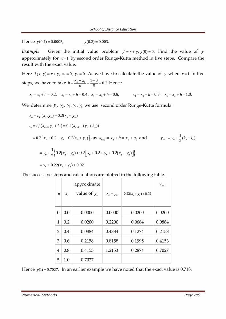
School of Distance Education
Numerical Methods Page 205
Hence (0.1) 0.0005,y (0.2) 0.003.y
Example Given the initial value problem , (0) 0.y x y y Find the value of y
approximately for 1x by second order Runge-Kutta method in five steps. Compare theresult with the exact value.
Here 0 0( , ) , 0, 0.f x y x y x y As we have to calculate the value of y when 1x in five
steps, we have to take 0 1 00.2.
5nx x
hn
Hence
1 0 2 1 3 20.2, 0.4, 0.6,x x h x x h x x h 4 3 5 40.8, 1.0.x x h x x h
We determine 1 2 3 4 5, , , ,y y y y y we use second order Runge-Kutta formula:
( , ) 0.2( )n n n n nk hf x y x y
1 1 1( , ) 0.2( ( ))n n n n n nl hf x y k x y k
0.2 0.2 0.2( )n n n nx y x y , as 1 2n n nx x h x a and 1
1( )
2n n n ny y k l
10.2( ) 0.2 0.2 0.2( )
2n n n n n n ny x y x y x y
0.22( ) 0.02n n ny x y
The successive steps and calculations are plotted in the following table.
n nx
approximate
value of ny n nx y 0.22( ) 0.02n nx y
1ny
0 0.0 0.0000 0.0000 0.0200 0.0200
1 0.2 0.0200 0.2200 0.0684 0.0884
2 0.4 0.0884 0.4884 0.1274 0.2158
3 0.6 0.2158 0.8158 0.1995 0.4153
4 0.8 0.4153 1.2153 0.2874 0.7027
5 1.0 0.7027
Hence (1) 0.7027.y In an earlier example we have noted that the exact value is 0.718.
School of Distance Education
Numerical Methods Page 206
Exercises
In Exercises 1-10, solve the initial value problem using second order Runge-Kutta methodfor value of y at the given point of x with given .h
1. 1 , (0) 0dy
y ydx at the point 0.2x (Take 0.1).h
2. , (0) 11
dy y xy
dx x
at the point 0.1x (Take 0.02).h
3. , (0) 1.5yy x y at the point 0.2x (Take 0.1).h
4. , (0) 1dy
x y ydx at the point 0.2x (Take 0.1).h
5. , (0) 1y x y xy y at the point 0.1x (Take 0.02).h
6. 21 , (0) 0dy
y ydx at the point 0.4x (Take 0.2).h
7. , (0) 1dy
xy ydx at the point 0.4x (Take 0.2).h
8. 1 ln( ), (0) 1dy
x y ydx at the point 0.2x (Take 0.1).h
9. 2 , (0) 1y x y y at the point 0.1x (Take 0.05).h
10. 2 , (0) 1y xy y at the point 0.5x (Take 0.1).h
In Exercises 11-13, apply second order Runge-Kutta method. Do 10 steps.
11. , (0) 1, 0.1y y y h
12. 2 , (0) 0.5, 0.1y y y y h
13. 22(1 ), (0) 0, 0.05y y y h
14. 22 0, (0) 1, 0.2y xy y h
15. Solve using second order Runge-Kutta method ( )y x y y x with (0) 2y for therange 0.00(0.02)0.06.
16. Solve using second order Runge-Kutta method 2xy y
y with 1y at 0x for
0.5h on the interval [0, 1].
School of Distance Education
Numerical Methods Page 207
17. Using second order Runge-Kutta method find (0.2)y of the initial value problem2 , (0) 1,y x y y taking 0.1.h
18. Using second order Runge-Kutta method find the value of y at the point 2x in
steps of 0.2 of the initial value problem 2 , (1) 1dy
xy ydx .
Fourth Order Runge-Kutta method
The Runge-Kutta method1 of fourth order (also known as classical Runge-Kuttamethod) gives greater accuracy and is most widely used for finding the approximatesolution of first order ordinary differential equations. The method is well suited forcomputers. The method is shown in the following algorithm.
Algorithm (The Runge-Kutta method)
Given the initial value problem (1). Suppose 0 1 2, , ,x x x be equally spaced x values withinterval .h i.e.,
1 0 2 1, ,x x h x x h
Also denote 0 0 1 1 2 2( ), ( ), ( ),y y x y y x y y x
For 0, 1,n , until termination do:
1n nx x h
( , )n n nA hf x y …(11)
1 12 2( , )n n n nB hf x h y A …(12)
1 12 2( , )n n n nC hf x h y B …(13)
( , )n n n nD hf x h y C …(14)
1
1( 2 2 )
6n n n n n ny y A B C D …(15)
Example Use Runge-Kutta method with 0.1h to find (0.2)y given 22 yxdx
dy with
(0) 0.y
Here 2 20 0( , ) , 0, 0, 0.1.f x y x y x y h Hence
1 0 2 10.1, 0.2.x x h x x h
To determine 1 2,y y we use improved Euler formula. Using Eqs. (12) (15),
1 0.1n n nx x h x
School of Distance Education
Numerical Methods Page 208
2 2( , ) 0.1( )n n n n nA hf x y x y
221 1 12 2 2( , ) 0.1 ( 0.05)n n n n n n nB hf x h y A x y A
221 1 12 2 2( , ) 0.1 ( 0.05)n n n n n n nC hf x h y B x y B
221( , ) 0.1n n n n n n nD hf x h y C x y C
1
1( 2 2 )
6n n n n n ny y A B C D
1 0 0.1 0 0.1 0.1x x
2 2 2 20 0 00.1( ) 0.1(0 0 ) 0A x y
22 10 0 0 020.1 ( 0.05)B x y A
2 20.1 (0.05) 0 0.00025.
22 10 0 0 020.1 ( 0.05)C x y B
2 20.1 (0.05) (0.000125) 0.00025.
220 1 0 00.1D x y C
2 20.1 (0.1) (0.00025) 0.001.
1 0 0 0 0 0
1( 2 2 )
6y y A B C D
10 (0 2 0.00025 2 0.00025 0.001) 0.00033.
6
2 1 0.1 0.1 0.1 0.2x x
2 2 2 21 1 10.1( ) 0.1 (0.1) (0.00033) 0.001A x y
22 11 1 1 120.1 ( 0.05)B x y A
2 20.1 (0.15) (0.00083) 0.00225.
22 11 1 1 120.1 ( 0.05)C x y B
2 20.1 (0.15) (0.001455) 0.00025.
School of Distance Education
Numerical Methods Page 209
221 2 1 10.1D x y C
2 20.1 (0.2) (0.0058) 0.004.
2 1 1 1 1 1
1( 2 2 )
6y y A B C D
10.00033 (0.014) 0.002663.
6
Example Use Runge-Kutta method with 0.2h to find the value of y at 0.2,x 0.4,x
and 0.6,x given 21 , (0) 0.dy
y ydx
Here 20 0( , ) 1 , 0, 0, 0.2.f x y y x y h Hence
1 0 2 10.2, 0.4.x x h x x h
To determine 1 2,y y we use improved Euler formula:
1 0.2n n nx x h x
2( , ) 0.2(1 )n n n nA hf x y y
21 1 12 2 2( , ) 0.2 1n n n n n nB hf x h y A y A
21 1 12 2 2( , ) 0.2 1n n n n n nC hf x h y B y B
2( , ) 0.2 1n n n n n nD hf x h y C y C
1
1( 2 2 )
6n n n n n ny y A B C D
1 0 0.2 0 0.2 0.2x x
2 20 00.2(1 ) 0.2(1 0 ) 0.2A y
210 0 020.2 1B y A
20.2 1 (0.1) 0.202.
210 0 020.2 1C y B
20.2 1 (0.101) 0.20204.
20 0 00.2 1D y C
20.2 1 (0.20204) 0.20816.
School of Distance Education
Numerical Methods Page 210
1 0 0 0 0 0
1( 2 2 )
6y y A B C D
10 (0.2 2 0.202 2 0.20204 0.20816) 0.2027.
6
i.e., (0.2) 0.2027.y
2 1 0.1 0.2 0.2 0.4x x
2 21 10.2(1 ) 0.2 1 (0.2027) 0.2082A y
211 1 120.2 1B y A
20.2 1 (0.3068) 0.2188.
211 1 120.2 1C y B
20.2 1 (0.3121) 0.2195. 21 1 10.2 1D y C 20.2 1 (0.4222) 0.2356.
2 1 1 1 1 1
1( 2 2 )
6y y A B C D
10.00033 (0.2082 2 0.2195 2 0.2195 0.2356)
6
0.4228.
i.e., (0.4) 0.4228,y correct to four decimal places.
3 2 0.1 0.4 0.2 0.6x x
22 20.2(1 );A y 21
2 2 220.2 1 ;B y A
212 2 220.2 1 ;C y B 22 2 20.2 1 .D y C
Substituting the values, and using
3 2 2 2 2 2
1( 2 2 )
6y y A B C D
we obtain 3(0.6) 0.6841,y y correct to four decimal places.
Example Given the initial value problem , (0) 0.y x y y Find the value of y
approximately for 1x by Runge-Kutta method in five steps. Compare the result with theexact value.
Here 0 0( , ) , 0, 0.f x y x y x y As we have to calculate the value of y when 1x in five
steps, we have to take 0 1 00.2.
5nx x
hn
Hence
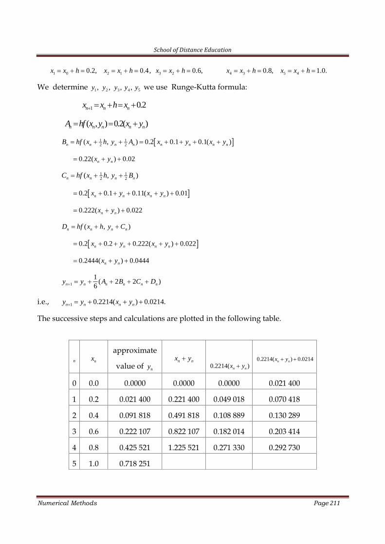
School of Distance Education
Numerical Methods Page 211
1 0 2 1 3 20.2, 0.4, 0.6,x x h x x h x x h 4 3 5 40.8, 1.0.x x h x x h
We determine 1 2 3 4 5, , , ,y y y y y we use Runge-Kutta formula:
1 0.2n n nx x h x
( , ) 0.2( )n n n n nA hf x y x y
1 12 2( , ) 0.2 0.1 0.1( )n n n n n n n nB hf x h y A x y x y
0.22( ) 0.02n nx y
1 12 2( , )n n n nC hf x h y B
0.2 0.1 0.11( ) 0.01n n n nx y x y
0.222( ) 0.022n nx y
( , )n n n nD hf x h y C
0.2 0.2 0.222( ) 0.022n n n nx y x y
0.2444( ) 0.0444n nx y
1
1( 2 2 )
6n n n n n ny y A B C D
i.e., 1 0.2214( ) 0.0214.n n n ny y x y
The successive steps and calculations are plotted in the following table.
n nxapproximate
value of nyn nx y
0.2214( )n nx y0.2214( ) 0.0214n nx y
0 0.0 0.0000 0.0000 0.0000 0.021 400
1 0.2 0.021 400 0.221 400 0.049 018 0.070 418
2 0.4 0.091 818 0.491 818 0.108 889 0.130 289
3 0.6 0.222 107 0.822 107 0.182 014 0.203 414
4 0.8 0.425 521 1.225 521 0.271 330 0.292 730
5 1.0 0.718 251
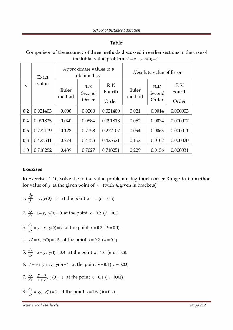
School of Distance Education
Numerical Methods Page 212
Table:
Comparison of the accuracy of three methods discussed in earlier sections in the case ofthe initial value problem , (0) 0.y x y y
nx
Exactvalue
Approximate values to yobtained by
Absolute value of Error
Eulermethod
R-KSecondOrder
R-KFourth
Order
Eulermethod
R-KSecondOrder
R-KFourth
Order
0.2 0.021403 0.000 0.0200 0.021400 0.021 0.0014 0.000003
0.4 0.091825 0.040 0.0884 0.091818 0.052 0.0034 0.000007
0.6 0.222119 0.128 0.2158 0.222107 0.094 0.0063 0.000011
0.8 0.425541 0.274 0.4153 0.425521 0.152 0.0102 0.000020
1.0 0.718282 0.489 0.7027 0.718251 0.229 0.0156 0.000031
Exercises
In Exercises 1-10, solve the initial value problem using fourth order Runge-Kutta methodfor value of y at the given point of x (with .h given in brackets)
1. , (0) 1dy
y ydx at the point 1x ( 0.5)h
2. 1 , (0) 0dy
y ydx at the point 0.2x ( 0.1).h
3. , (0) 2dy
y x ydx at the point 0.2x ( 0.1).h
4. , (0) 1.5yy x y at the point 0.2x ( 0.1).h
5. , (1) 0.4dy
x y ydx at the point 1.6x (e 0.6).h
6. , (0) 1y x y xy y at the point 0.1x ( 0.02).h
7. , (0) 11
dy y xy
dx x
at the point 0.1x ( 0.02).h
8. , (1) 2dy
xy ydx at the point 1.6x ( 0.2).h
School of Distance Education
Numerical Methods Page 213
9. 1 ln( ), (0) 1dy
x y ydx at the point 0.2x ( 0.1).h
10. 2 , (0) 1y x y y at the point 0.1x ( 0.05).h
11. 2 , (0) 1y xy y at the point 0.5x ( 0.1).h
12. 13 , (0) 1
2y x y at the point 0.2x ( 0.05).h
13. Solve using Runge-Kutta method ( )y x y y x with (0) 2y for the range0.00(0.02)0.06.
14. Using Runge-Kutta method find (0.2)y of the initial value problem 2 2 , (0) 0,y x y y
taking 0.2.h
15. Using Runge-Kutta method find the value of y at the point 2x in steps of 0.2 of the
initial value problem 2 , (1) 1dy
xy ydx .
16. Using Runge-Kutta method find (1.3),y given 2y x y and (1) 2.y Take 0.3h .
17. Solve using Runge-Kutta method 2xy y
y with 1y at 0x for 0.5h on the
interval [0, 1].
18. Solve 1 12 ln , (1) 0y x y x x y for 1 1.8x
(a) by Euler method with 0.1.h
(b) by improved Euler method with 0.2.h
(c) by Runge-Kutta method with 0.4.h
(d) Compare the above results with the exact value. Determine the errors. Comment.
School of Distance Education
Numerical Methods Page 214
18
PREDICTOR CORRECTOR METHODS
Introduction
Euler method and fourth order Runge-Kutta methods are called single-step methods,where we have seen that the computation of 1ny requires the knowledge of ny only. Butmodified Euler method is a multi-step method since for the computation of 1ny theknowledge of ny is not enough. It is a predictor-corrector method, in which a predictorformula is used to predict the value 1ny of y at 1nx and then a corrector formula is used toimprove the value of 1ny .
For example, consider the initial value problem
0 0, , ( ) .dy
f x y y x ydx
Using simple Euler’s and modified Euler’s method, we can write down a simplepredictor-corrector pair (P-C) as
:P(0)
1 ( , ).n n n ny y hf x y
:C(1) (0)
1 1 1( , ) ( , ) .2n n n n n nhy y f x y f x y
Here, (1)1ny is the first corrected value of 1.ny . The corrector formula may be used
iteratively as defined below:
( ) ( 1)1 1 1( , ) ( , ) 1, 2,
2r r
n n n n n nhy y f x y f x y r
The iteration terminate when two successive iterates agree to the desired accuracy. Wehave considered modified Euler method in the previous chapter.
In this chapter we consider two methods: Adams-Moulton and Milne’s Methods.They require function values at 1 2, , ,n n nx x x for the computation of the function value at
1.nx
Adams-Moulton Method
Consider the initial value problem
0 0( , ), ( ) .y f x y y x y …(1)
School of Distance Education
Numerical Methods Page 215
Starting with given 0x and given the step size h , we have
1 0 1 0 2 0, , 2 ,x x h x x h x x h and 3 0 3x x h . We denote
0 0 0 1 1 1 1 1 1 2 2 2( , ), ( , ), ( , ), ( , ),f f x y f f x y f f x y f f x y and 3 3 3( , ).f f x y
In Adams-Moulton Method, we predict by
1 0 0 1 2 3(55 59 37 9 )24
P hy y f f f f …(1)
and correct by
1 0 1 0 1 2(9 19 5 ),24
C phy y f f f f …(2)
where 1 1 1( , ).p Pf f x y
The general forms for formulae (1) and (2) are given by
1 1 2 3(55 59 37 9 )24
Pn n n n n n
hy y f f f f …(1)
with correction
1 1 1 2(9 19 5 ),24
C pn n n n n n
hy y f f f f …(2)
where 1 1 1( , ).p Pn n nf f x y
The formulae given above are example of explicit predictor –corrector formulae as they areexpressed in ordinate form.
Example Given 21 ; (0) 0.dy
y ydx Compute (0.8)y using Adams-Moulton Method.
Here 1 0.8, 0.2.x h Hence 0 1 0.8 0.2 0.6,x x h
1 0 0.4,x x h 2 0 2 0.2,x x h and 3 0 3 0.x x h
The starter values are (0.6), (0.4)y y and (0.2)y . Using fourth-order Runge-Kutta method(Ref. Example 7 in the previous chapter), the values are found to be:
(0.6) 0.6841, (0.4) 0.4228, (0.2) 0.2027.y y y
Hence 0 0 1 1( ) (0.6) 0.6841, ( ) (0.4) 0.4228,y y x y y y x y
2 0.2027y and 3 3( ) (0) 0.y y x y
Also, 2 20 0 0 0( , ) 1 1 (0.6841)f f x y y ;
School of Distance Education
Numerical Methods Page 216
2 21 1 1 1( , ) 1 1 (0.4228)f f x y y ;
and so on. We tabulate them below:
x y 2( ) 1f x y
3 0.0x
2 0.2x
1 0.4x
0 0.6x
3y 0.000
2y 0.2027
1y 0.4228
0y 0.6841
3f 1.0000
2f 1.0411
1f 1.1787
0f 1.4681
Substituting these values in (1), we obtain the predicted value of 1y at 1 0.8x as
2 21
0.20.6841 55[1 (0.6841) ] 59[1 (0.4228) ]
24Py
237[1 (0.4228) ] 9
1.0233, on simplification.
Corrected value of 1y at 1 0.8x is obtained using (2) as below:
2 21
0.20.6841 9[1 (0.0233) ] 19[1 (0.6841) ]
24Cy
2 25[1 (0.4228) ] [1 (0.2027) ]
1.0296, on simplification.
Exercises
1. Using Adams-Moulton predictor-corrector method, find the value of y at 4.4x fromthe differential equation
25 2,dy
x ydx
given that
4.0 4.1 4.2 4.3
1.0000 1.0049 1.0097 1.0143
x
y
2. Using Adams-Moulton predictor-corrector method, find the value of y at 0.8,x and1.0x of the initial value problem
2 , (0) 1dy
y x ydx
School of Distance Education
Numerical Methods Page 217
(Take 0.2.)h
3. Using Adams-Moulton predictor-corrector method, find the value of y at 1.4x of theinitial value problem
2 1, (1) 1.0x y xy y
with starter values (1.1) 0.996, (1.2) 0.986, (1.3) 0.972.y y y
4. Find the solution of the initial value problem2 sin , (0) 1y y t y
using Adams-Moulton predictor-corrector method, in the interval (0.2, 0.5) given that
(0.05) 1.00125, (0.1) 1.00502, (0.15) 1.01136.y y y
Milne’s Method
Consider the initial value problem
0 0( , ), ( ) .y f x y y x y …(1)
Starting with given 0x and given the step size h , we have
1 0 1 0 2 0, , 2 ,x x h x x h x x h and 3 0 3x x h . We denote
0 0 0 1 1 1 1 1 1 2 2 2( , ), ( , ), ( , ), ( , ),f f x y f f x y f f x y f f x y and 3 3 3( , ).f f x y
In Milne’s Method, we predict by
1 3 2 1 0
4(2 2 )
3P h
y y f f f …(1)
and correct by
1 1 1 0 1( 4 ),3
C Phy y f f f …(2)
where 1 1 1( , ).P Pf f x y
The general forms for formulae (1) and (2) are given by
1 3 2 1
4(2 2 )
3Pn n n n n
hy y f f f …(3)
and correct by
1 1 1 1( 4 ),3
C Pn n n n n
hy y f f f …(4)
School of Distance Education
Numerical Methods Page 218
where 1 1 1( , ).P Pn n nf f x y
The formulae given above is also explicit predictor –corrector formulae as they areexpressed in ordinate form.
Example Given 21 ; (0) 0.dy
y ydx Compute (0.8)y and (1.0)y using Milne’s Method.
Solution
Determination of (0.8) :y
Here take 1 0.8, 0.2.x h Hence
0 1 0.8 0.2 0.6,x x h 1 0.4,x 2 0.2,x 3 0.x
The starter values are (0.6), (0.4)y y and (0.2)y . Using fourth-order Runge-Kutta method,the valued are found to be:
(0.6) 0.6841, (0.4) 0.4228, (0.2) 0.2027.y y y
Hence
0 1 20.6841, 0.4228, 0.2027y y y and
3 3( ) (0) 0.y y x y
Also, 2 20 0 0 0( , ) 1 1 (0.6841)f f x y y ;
2 21 11 1 (0.4228)f y ;
and so on. We tabulate them below:
x y 2( ) 1f x y
3 0.0x
2 0.2x
1 0.4x
0 0.6x
3y 0.000
2y 0.2027
1y 0.4228
0y 0.6841
3f 1.0000
2f 1.0411
1f 1.1787
0f 1.4681
Substituting these values in (1), we obtain the predicted value of 1y at 1 0.8x as
1
0.80 2(1.0411) 1.1787 2(1.4681) 1.0239
3Py
Hence 2 21 11 1 (1.0239) 2.0480Pf y
School of Distance Education
Numerical Methods Page 219
and hence the corrected value of 1y at 1 0.8x is obtained using (2) as below:
1
0.20.4228 1.1787 4(1.4681) 2.0480 1.0294.
3Cy
Hence (0.8) 1.0294,y correct to four places of decimal.
Determination of (1.0) :y
Here take 1 1.0, 0.2.x h Hence
0 1 1.0 0.2 0.8,x x h 1 0.6,x 2 0.4,x 3 0.2.x
The starter values are (0.8), (0.6),y y and (0.4)y . We have the values
(0.8) 1.0294,y (0.6) 0.6841, (0.4) 0.4228.y y
Hence
0 1 21.0294, 0.6841, 0.4228y y y and 3 0.y
Also, 2 20 01 1 (1.0294)f y ; 2 2
1 11 1 (0.6841)f y ; and so on.
x y 2( ) 1f x y
3 0.2x
2 0.4x
1 0.6x
0 0.8x
3y 0.2027
2y 0.4228
1y 0.6841
0y 1.0294
3f 1.0411
2f 1.1787
1f 1.4681
0f 2.0597
Substituting these values in (1), we obtain the predicted value of 1y at 1 1.0x as
1 1.5384Py
Hence 21 11 3.3667Pf y
Corrected value of 1y at 1 0.8x is obtained using (2) as below:
1 1.5557.Cy
Example Find, using Milne’s predictor-corrector method, (2.0)y if ( )y x is the solution of
2
yx
dx
dy
School of Distance Education
Numerical Methods Page 220
assuming (0) 2. (0.5) 2.636, (1.0) 3.595y y y and (1.5) 4.968.y
Here take 1 2.0, 0.5.x h Hence
0 1 2.0 0.5 1.5,x x h 1 1,x 2 0.5,x 3 0.x
Also, by the assumption,
0 1 24.968, 3.595, 2.636y y y and 3 2.y
As ( , ) ,2
x yf x y
we have
0 00 0 0
1.5 4.968( , ) 3.2340.
2 2
x yf f x y
;
1 11 1 1
1.0 3.595( , ) 2.2975.
2 2
x yf f x y
;
2 22 2 2
0.5 2.636( , ) 1.5680.
2 2
x yf f x y
;
Now, using predictor formula we compute
1 3 2 1 0
42 2
3P h
y y f f f
4 0.52 2 1.5680 2.2975 2 3.2340 6.8710.
3
Using the predicted value, we shall compute the corrected value of 1y from the correctorformula
1 1 1 0 1( 4 ),3
C Phy y f f f (2)
where 1 1 1( , ).P Pf f x y
Now using the available predicted value 1Py ,
1 11 1 1
2 6.871( , ) 4.4355.
2 2
PP P x y
f f x y
Thus the corrected value is given by
1
0.53.595 2.2975 4 3.234 4.4355 6.8731667.
3Cy
Hence an approximate value of y at 2x is taken as 1(2) 6.8731667.Cy y
School of Distance Education
Numerical Methods Page 221
Example Tabulate the solution of
10; yyxdx
dy
in the interval 0 x 0.4, with h = 0.1, using Milne’s predictor-corrector method.
We take 1 0.4.x We cannot immediately use Milne’s predictor-corrector method as itneed the value of y at the previous four points 0 1 0.4 0.1 0.3,x x h 1 0.2,x
2 0.1,x 3 0.x Clearly, 3 3( ) (0) 1.y y x y For the calculation of the rest three y valueswe use Runge-Kutta method of fourth order and then switch over to Milne’s P-C method.
By Runge-Kutta method of fourth order it can be seen that (work is left as an exercise)
0 0( ) (0.3) 1.3997,y y x y 1 1( ) (0.2) 1.2428,y y x y 2 2( ) (0.1) 1.1103.y y x y
From the given differential equation ( , )f x y x y , and we have
0 0 0 0 0, 0.3 1.3997 1.6997.f f x y x y
1 1 1 1 1, 0.2 1.2428 1.4428.f f x y x y
2 2 2 2 2, 0.1 1.1103 1.2103.f f x y x y
Now, using predictor formula we compute
1 3 2 1 0
42 2
3P h
y y f f f
4 0.51 2 1.2103 1.4428 2 1.6997 1.58363
3
Before using the corrector formula
1 1 1 0 1( 4 ),3
C Phy y f f f …(2)
we compute
1 1 1 1 1( , ) 0.4 1.5836 1.9836.P P Pf f x y x y
Hence
1
0.11.2428 1.4428 4 1.6997 1.9836 1.5836.
3Cy
School of Distance Education
Numerical Methods Page 222
The required solution is tabulated below:
x 0 0.1 0.2 0.3 0.4
y 1.0000 1.1103 1.2428 1.3997 1.5836
Example Find, using Milne’s predictor-corrector method, (2.0)y if ( )y x is the solution of
2
yx
dx
dy assuming (0) 2. (0.5) 2.636, (1.0) 3.595y y y and (1.5) 4.968.y
Here take 1 2.0, 0.5.x h Hence
0 1 2.0 0.5 1.5,x x h 1 1,x 2 0.5,x 3 0.x
Also, by the assumption,
0 1 24.968, 3.595, 2.636y y y and 3 2.y
As ( , ) ,2
x yf x y
we have
0 00 0 0
1.5 4.968( , ) 3.2340.
2 2
x yf f x y
;
1 11 1 1
1.0 3.595( , ) 2.2975.
2 2
x yf f x y
;
2 22 2 2
0.5 2.636( , ) 1.5680.
2 2
x yf f x y
;
Now, using predictor formula we compute
1 3 2 1 0
42 2
3P h
y y f f f
4 0.52 2 1.5680 2.2975 2 3.2340 6.8710.
3
Using the predicted value, we shall compute the corrected value of 1y from the correctorformula
1 1 1 0 1( 4 ),3
C Phy y f f f
where 1 1 1( , ).P Pf f x y
Now using the available predicted value 1Py ,
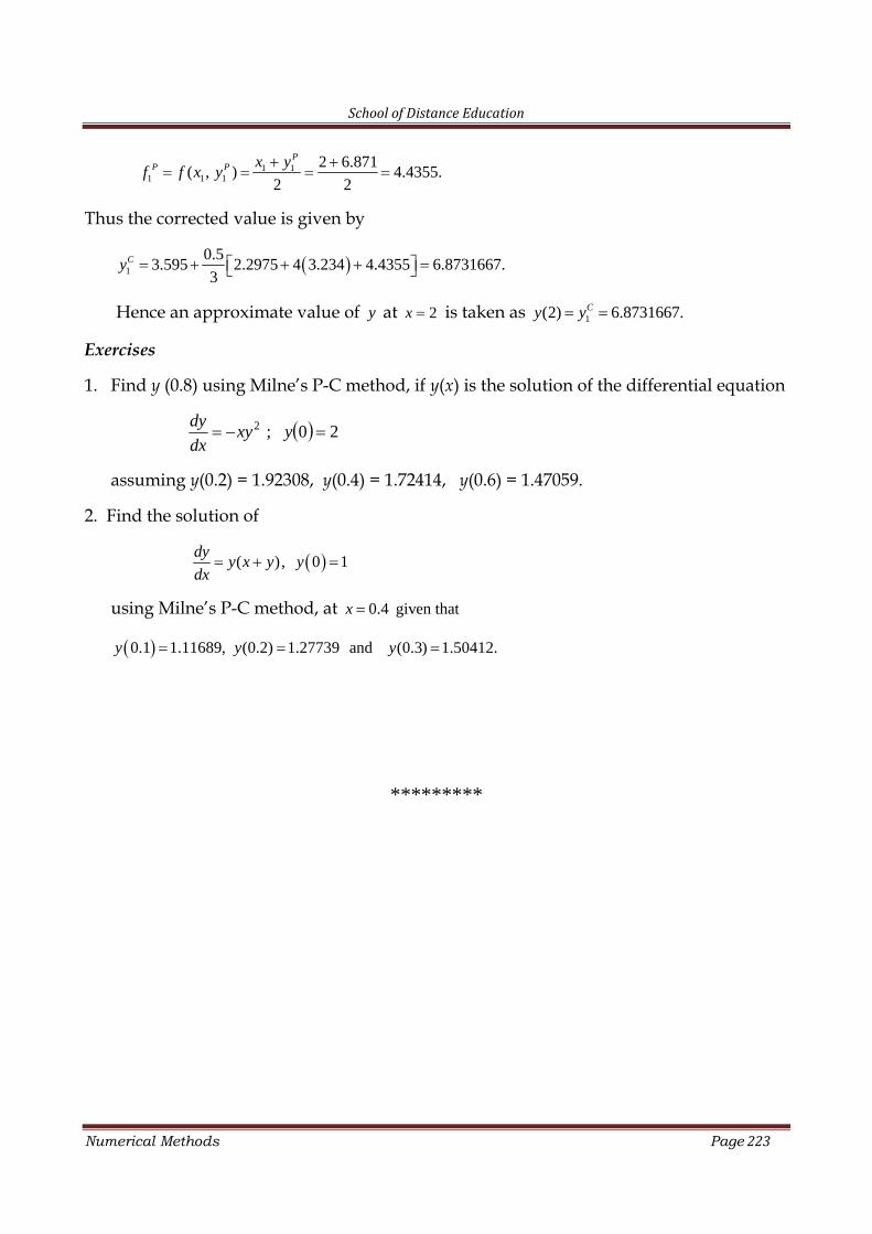
School of Distance Education
Numerical Methods Page 223
1 11 1 1
2 6.871( , ) 4.4355.
2 2
PP P x y
f f x y
Thus the corrected value is given by
1
0.53.595 2.2975 4 3.234 4.4355 6.8731667.
3Cy
Hence an approximate value of y at 2x is taken as 1(2) 6.8731667.Cy y
Exercises
1. Find y (0.8) using Milne’s P-C method, if y(x) is the solution of the differential equation
20;2 yxydx
dy
assuming y(0.2) = 1.92308, y(0.4) = 1.72414, y(0.6) = 1.47059.
2. Find the solution of
( ), 0 1dy
y x y ydx
using Milne’s P-C method, at 0.4 given thatx
0.1 1.11689, (0.2) 1.27739 andy y (0.3) 1.50412.y
*********