2.2 gaussian elimination with scaled partial pivoting€¦ · 2.2 gaussian elimination with scaled...
TRANSCRIPT

120202: ESM4A - Numerical Methods 87
Visualization and Computer Graphics LabJacobs University
2.2 Gaussian Elimination with ScaledPartial Pivoting
120202: ESM4A - Numerical Methods 88
Visualization and Computer Graphics LabJacobs University
Observation
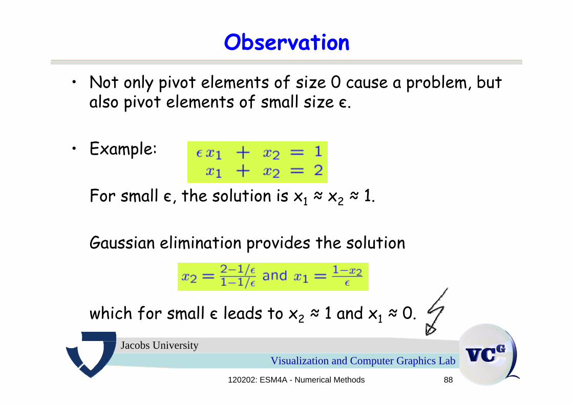
• Not only pivot elements of size 0 cause a problem, butalso pivot elements of small size є.
• Example:
For small є, the solution is x1 ≈ x2 ≈ 1.
Gaussian elimination provides the solution
which for small є leads to x2 ≈ 1 and x1 ≈ 0.

120202: ESM4A - Numerical Methods 89
Visualization and Computer Graphics LabJacobs University
Pivoting
• Observation: Pivot element of last row is never used.• Idea: Switch order of rows.
• Example revisited:Reordering:
Solution:
This is correct, even for small є (and even for є = 0).

120202: ESM4A - Numerical Methods 90
Visualization and Computer Graphics LabJacobs University
Vandermonde revisited
• There was no small value є in the equation system.• Why was it ill-conditioned?• Ratio in the first row of the matrix was
• It is not the absolute size that matters but therelative size!

120202: ESM4A - Numerical Methods 91
Visualization and Computer Graphics LabJacobs University
Scaled partial pivoting
• Process the rows in the order such that the relative pivot element size is largest.
• The relative pivot element size is given by the ratioof the pivot element to the largest entry in (the left-hand side of) that row.
120202: ESM4A - Numerical Methods 92
Visualization and Computer Graphics LabJacobs University
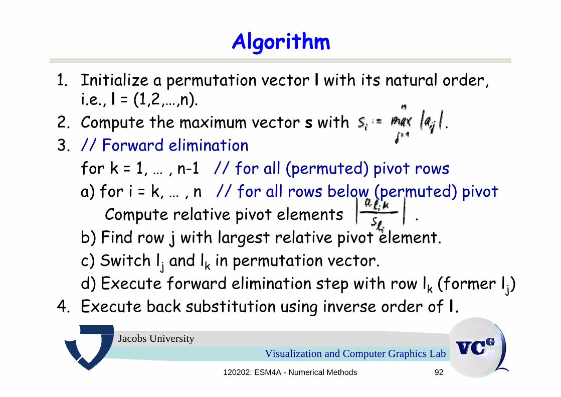
Algorithm1. Initialize a permutation vector l with its natural order,
i.e., l = (1,2,…,n).2. Compute the maximum vector s with .3. // Forward elimination
for k = 1, … , n-1 // for all (permuted) pivot rowsa) for i = k, … , n // for all rows below (permuted) pivot
Compute relative pivot elements .b) Find row j with largest relative pivot element.c) Switch lj and lk in permutation vector.d) Execute forward elimination step with row lk (former lj)
4. Execute back substitution using inverse order of l.

120202: ESM4A - Numerical Methods 93
Visualization and Computer Graphics LabJacobs University
Examplesystem:
initialization:permutation vector l = (1,2,3,4)maximum vector s = (13,18,6,12)
1st iteration: l1 = 1relative pivot elements: l = (3,2,1,4)Execute first forward elimination step for l1 = 3.
120202: ESM4A - Numerical Methods 94
Visualization and Computer Graphics LabJacobs University
Example
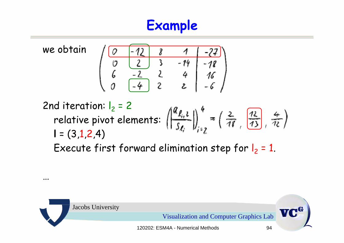
we obtain
2nd iteration: l2 = 2relative pivot elements: l = (3,1,2,4)Execute first forward elimination step for l2 = 1.
…
120202: ESM4A - Numerical Methods 95
Visualization and Computer Graphics LabJacobs University
Example
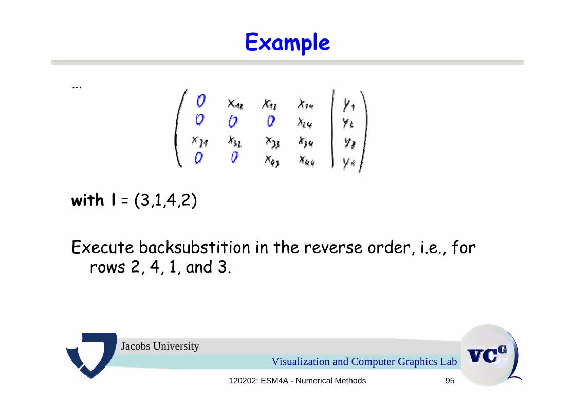
…
with l = (3,1,4,2)
Execute backsubstition in the reverse order, i.e., forrows 2, 4, 1, and 3.
120202: ESM4A - Numerical Methods 96
Visualization and Computer Graphics LabJacobs University
Remark
• Gaussian elimation with scaled partial pivoting alwaysworks, if a unique solution exists.
• A square linear equation system has a unique solution, if the left-hand side is a non-singular matrix.
• A non-singular matrix is also referred to as regular.• A non-singular matrix has an inverse matrix.• A non-singular matrix has full rank.
120202: ESM4A - Numerical Methods 97
Visualization and Computer Graphics LabJacobs University
Checking non-singularity
• A square matrix is non-singular, iff its determinant isnon-zero.
• The Gaussian elimination algorithm (with or withoutscaled partial pivoting) will fail for a singular matrix(division by zero).
• We will never get a wrong solution, such that checkingnon-singularity by computing the determinant is notrequired.
• Non-singularity is implicitly verified by a successfulexecution of the algorithm.
120202: ESM4A - Numerical Methods 98
Visualization and Computer Graphics LabJacobs University
Time complexity
1. Initialize a permutation vector l with its natural order, i.e., l = (1,2,…,n).time complexity O(n)
2. Compute the maximum vector s.time complexity O(n2)
120202: ESM4A - Numerical Methods 99
Visualization and Computer Graphics LabJacobs University
Time complexity
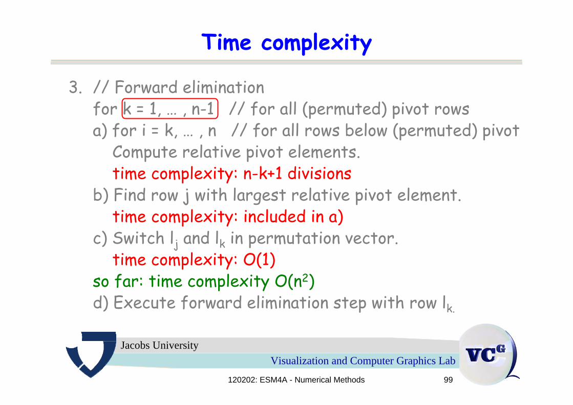
3. // Forward eliminationfor k = 1, … , n-1 // for all (permuted) pivot rowsa) for i = k, … , n // for all rows below (permuted) pivot
Compute relative pivot elements.time complexity: n-k+1 divisions
b) Find row j with largest relative pivot element.time complexity: included in a)
c) Switch lj and lk in permutation vector.time complexity: O(1)
so far: time complexity O(n2)d) Execute forward elimination step with row lk.
120202: ESM4A - Numerical Methods 100
Visualization and Computer Graphics LabJacobs University
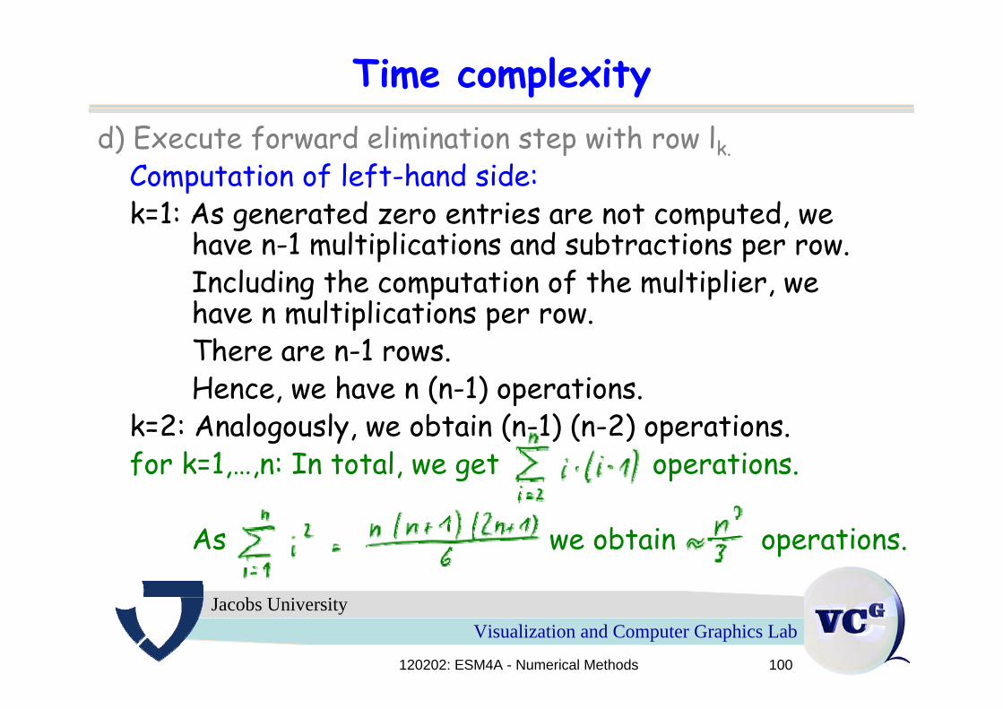
Time complexityd) Execute forward elimination step with row lk.
Computation of left-hand side:k=1: As generated zero entries are not computed, we
have n-1 multiplications and subtractions per row.Including the computation of the multiplier, wehave n multiplications per row.There are n-1 rows. Hence, we have n (n-1) operations.
k=2: Analogously, we obtain (n-1) (n-2) operations.for k=1,…,n: In total, we get operations.
As we obtain operations.
120202: ESM4A - Numerical Methods 101
Visualization and Computer Graphics LabJacobs University
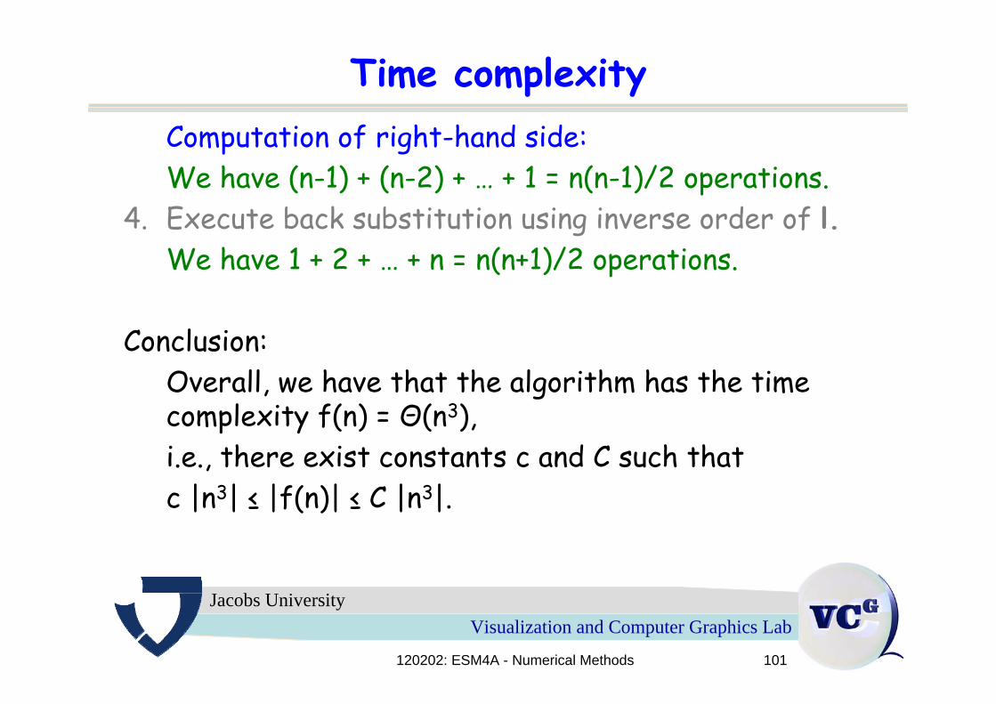
Time complexityComputation of right-hand side:We have (n-1) + (n-2) + … + 1 = n(n-1)/2 operations.
4. Execute back substitution using inverse order of l.We have 1 + 2 + … + n = n(n+1)/2 operations.
Conclusion: Overall, we have that the algorithm has the time complexity f(n) = Θ(n3), i.e., there exist constants c and C such thatc |n3| ≤ |f(n)| ≤ C |n3|.

120202: ESM4A - Numerical Methods 102
Visualization and Computer Graphics LabJacobs University
Remark
• The derived time complexity is not a worst-casescenario, but is what we always have to execute.
• Can we do better?• For special cases: yes!

120202: ESM4A - Numerical Methods 103
Visualization and Computer Graphics LabJacobs University
2.3 Banded Systems
120202: ESM4A - Numerical Methods 104
Visualization and Computer Graphics LabJacobs University
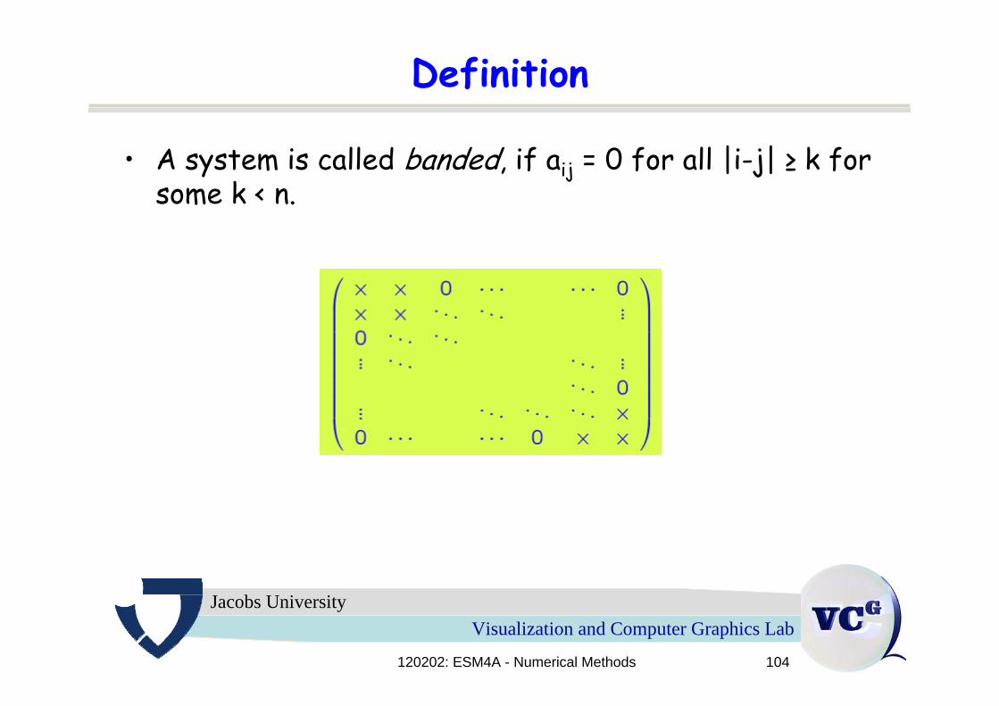
Definition
• A system is called banded, if aij = 0 for all |i-j| ≥ k forsome k < n.

120202: ESM4A - Numerical Methods 105
Visualization and Computer Graphics LabJacobs University
Example
• For k=2, the banded system is called tridiagonal.It is of the form
Gaussian elimination algorithm becomes simple.

120202: ESM4A - Numerical Methods 106
Visualization and Computer Graphics LabJacobs University
Gaussian elimination for tridiagonal system1. // Forward elimination:
for i = 2, … , n// all ai become 0 -> no need to compute// all ci do not change
2. // Backward substitution:
for i = n-1, … , 1

120202: ESM4A - Numerical Methods 107
Visualization and Computer Graphics LabJacobs University
Remarks
• The time complexity becomes Θ(n).
• The method can be generalized to any banded system.• Time complexity stays Θ(n).

120202: ESM4A - Numerical Methods 108
Visualization and Computer Graphics LabJacobs University
2.4 LU Decomposition
120202: ESM4A - Numerical Methods 109
Visualization and Computer Graphics LabJacobs University
Motivation
• In many applications, one does not have to solve a linear equation system for one object but for a large number.
• If the system is not banded, but has full entries, canwe still make computations faster as Θ(n3)?
• When solving a system for many objects, only theright-hand side changes.
• Hence, many computations stay the same. • We can make use of this.

120202: ESM4A - Numerical Methods 110
Visualization and Computer Graphics LabJacobs University
Example• In forward elimination, we execute the first step
• This can be written in the form
with

120202: ESM4A - Numerical Methods 111
Visualization and Computer Graphics LabJacobs University
Example• After this first step, we execute a second step
• This is equivalent to
with

120202: ESM4A - Numerical Methods 112
Visualization and Computer Graphics LabJacobs University
Example• After this second step, we execute a third step
• This is equivalent to
with
120202: ESM4A - Numerical Methods 113
Visualization and Computer Graphics LabJacobs University
Upper triangular matrix
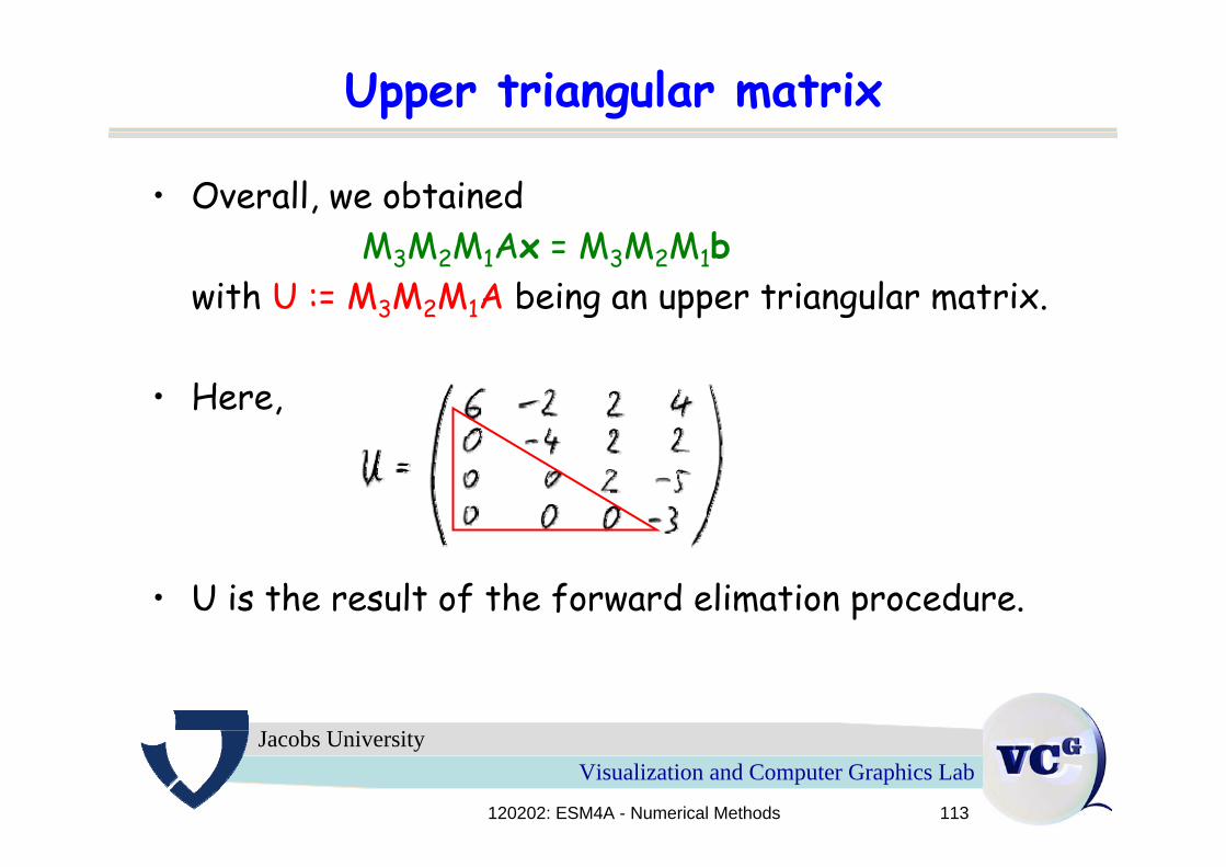
• Overall, we obtainedM3M2M1Ax = M3M2M1b
with U := M3M2M1A being an upper triangular matrix.
• Here,
• U is the result of the forward elimation procedure.

120202: ESM4A - Numerical Methods 114
Visualization and Computer Graphics LabJacobs University
Lower triangular matrix• Moreover, from U = M3M2M1A we get
A = (M3M2M1)-1U = M1-1M2
-1M3-1U
with L := M1-1M2
-1M3-1 being a lower triangular matrix.
• Here,
120202: ESM4A - Numerical Methods 115
Visualization and Computer Graphics LabJacobs University
Remarks
• L is a lower triangular matrix with entries 1 on thediagonal.
• Because of their simple structure, the inverse of thematrices M1, M2, and M3 is just the same matrix, where all non-zero entries below the diagonal becometheir additive inverse.
• Moreover, because of their simple structure, theproduct of the three matrices is obtain by just component-wise adding all non-zero entries below thediagonal.
• Hence, L can be directly retrieved from the forwardelimination step without further computations. Theentries are the negative Gaussian multipliers.