A NEW PIVOTING STRATEGY

FOR GAUSSIAN ELIMINATION

Markus OlschowkaInstitut fur Angewandte Mathematik

Universitat FreiburgD-79104 Freiburg

Germany

and

Arnold NeumaierAT&T Bell Laboratories600 Mountain Avenue

Murray Hill, NJ 07974-0636U.S.A.

email: neum@research.att.com

December 1993

Abstract.

This paper discusses a method for determining a good pivoting sequencefor Gaussian elimination, based on an algorithm for solving assignmentproblems. The worst case complexity is O(n3), while in practice O(n2.25)operations are sufficient.

1991 MSC Classification: 65F05 (secondary 90B80)

Keywords: Gaussian elimination, scaled partial pivoting, I-matrix, domi-nant transversal, assignment problem, bipartite weighted matching.

1

1 Introduction

For a system of linear equations Ax = b with a square nonsingularcoefficient matrix A, the most important solution algorithm is the systematicelimination method of Gauss. The basic idea of Gaussian elimination is thefactorization of A as the product LU of a lower triangular matrix L withones on its diagonal and an upper triangular matrix U , the diagonal entriesof which are called the pivot elements. In general, the numerical stabilityof triangularization is guaranteed only if the matrix A is symmetric positivedefinite, diagonally dominant, or an H-matrix.

In [4], p.159, Conte & deBoor write: It is “difficult (if not impossible) toascertain for a general linear system how various pivoting strategies affect theaccuracy of the computed solution. A notable and important exception tothis statement are the linear systems with positive definite coefficient matrix(...). For such a system, the error in the computed solution due to roundingerrors during elimination and back-substitution can be shown to be accept-ably small if the trivial pivoting strategy of no interchanges is used. But it isnot possible at present to give a “best” pivoting strategy for a general linearsystem, nor is it even clear what such a term might mean. (...) A currentlyaccepted strategy is scaled partial pivoting”.

Partial pivoting consists in choosing – when the kth variable is to be elimi-nated – as pivot element the element of largest absolute value in the remain-der of the kth column and exchanging the corresponding rows. For goodnumerical stability it is advisable to carry out the partial pivoting with priorscaling of the coefficient matrix A – i.e., replacing of A by D1AD2 , whereD1 and D2 are nonsingular diagonal matrices. To avoid additional roundingerrors the scaling is done implicitly: Let A = (aij) be an n×n -matrix andD1 = Diag(d11, ..., d

1n), then, in the jth reduction step A(j−1) → A(j), the

pivoting rule becomes:Find k ≥ j with

|a(j−1)kj | · d1k = max

i≥j|a

(j−1)ij | · d1i 6= 0,

and then take a(j−1)kj as pivot element.

The nonsingular diagonal matrix D1 must be chosen such that the triangu-larization with partial pivoting of D1AD2 is stable. (The matrix D2 doesnot affect the pivot choice, but is introduced for convenience.) The approach

2

to this problem taken by Wilkinson [13] is to insist that the scaled matrixbe equilibrated, i.e., all its rows have l1-norm 1. This can be achieved forarbitrary choice of D2, since the diagonal matrix D1 whose diagonal entriesare the inverse norms of the rows of AD2 is the unique diagonal matrix whichmakes D1AD2 equilibrated. The choice of D2 then determines D1 which inturn determines the pivot elements. In practice one usually takes for D2 theidentity matrix, D2 = I. However, this can be disastrous when the entriesin some row of A have widely differing magnitudes, and it is particularlyunsatisfactory for sparse matrices (Curtis & Reid [5]).One can improve the behavior by enforcing also that the transposed matrix isequilibrated, i.e., that all columns have norm 1. Ignoring the signs, the scaledmatrix is then doubly stochastic, i.e., the entries of each row and column sumto 1. Now the scaling matrices must satisfy nonlinear equations which arenot easy to solve. Parlett & Landis describe in [11] iterative proceduresfor scaling nonnegative matrices to double stochastic form, and they presentresults of tests comparing the new algorithms with other methods. How-ever, their examples suggest that their iterations require O(n4) operations,so these procedures are too slow to be useful as a scaling strategy for Gaus-sian elimination.

In the present paper we introduce a new idea for choosing the scaling matricesin such a way that A = D1AD2 has a structure resembling an equilibrated,diagonally dominant matrix. Thus, choosing D1 as the scaling matrix forimplicit partial pivoting, we expect better results in Gaussian eliminationthan with the traditional choices.

More precisely, we set ourselves the following task: Given the matrix A, finddiagonal matrices D1 and D2 such that A = D1AD2 has the following form:

(*) All coefficients are of absolute value at most 1 and there are n elementsof absolute value 1, no two of which lie in the same row or column.

In the special case when A is obtained by scaling and permuting a diagonallydominant matrix A0 it turns out that the triangular factorization of A usingpartial pivoting and implicit scaling with scaling factors determined by (*)chooses a pivot sequence equivalent to original ordering of A0. During re-duction those elements are taken as pivots, whose corresponding entries in Aare of absolute value 1. Thus the condition (*) recovers in this case the nat-ural stable ordering. The same happens for scaled and permuted symmetric

3

positive definite matrices. This nourishes the hope that we also get a goodpivoting sequence in the general situation. Although we cannot prove this,the experimental results obtained in Section 4 indeed suggest that this holds.

In Section 2 we investigate the properties of matrices with property (*) andof corresponding scaling matrices. In Section 3 we discuss in more detail theconsequences for pivoting. Section 4 describe the particular method we im-plemented to produce scaling factors such that the scaled matrix satisfies (*).The method involves at most O(n3) operations, i.e., the worst case work isof the same order as for the subsequent triangular factorization. Test resultswith some random matrices are given in Section 5.

Acknowledgment. I’d like to thank Carl de Boor and an unknown refereefor a number of useful remarks which helped to improve this paper.

2 Theoretical Foundations

Let A be an n×n -matrix and denote by Σ := Sym(n) the set of permutationsof 1, ..., n. For σ ∈ Σ, Pσ denotes the n×n - permutation matrix with entries

pij :=

{

1 if j = σ(i),0 otherwise.

PσA is obtained from A by permuting its rows in such a way that the ele-ments aσ(j),j are on its diagonal.

2.1. Lemma. If A is nonsingular, there exists at least one transversal forA.

Proof: Since

det(A) :=∑

σ∈Σ

sgn(σ)n∏

j=1

aσ(j),j 6= 0

there exists some σ ∈ Σ with∏n

j=1 aσ(j),j 6= 0. ✷

4

We call a matrix A structurally nonsingular if A has a transversal. A usefulcondition for this can be deduced from the

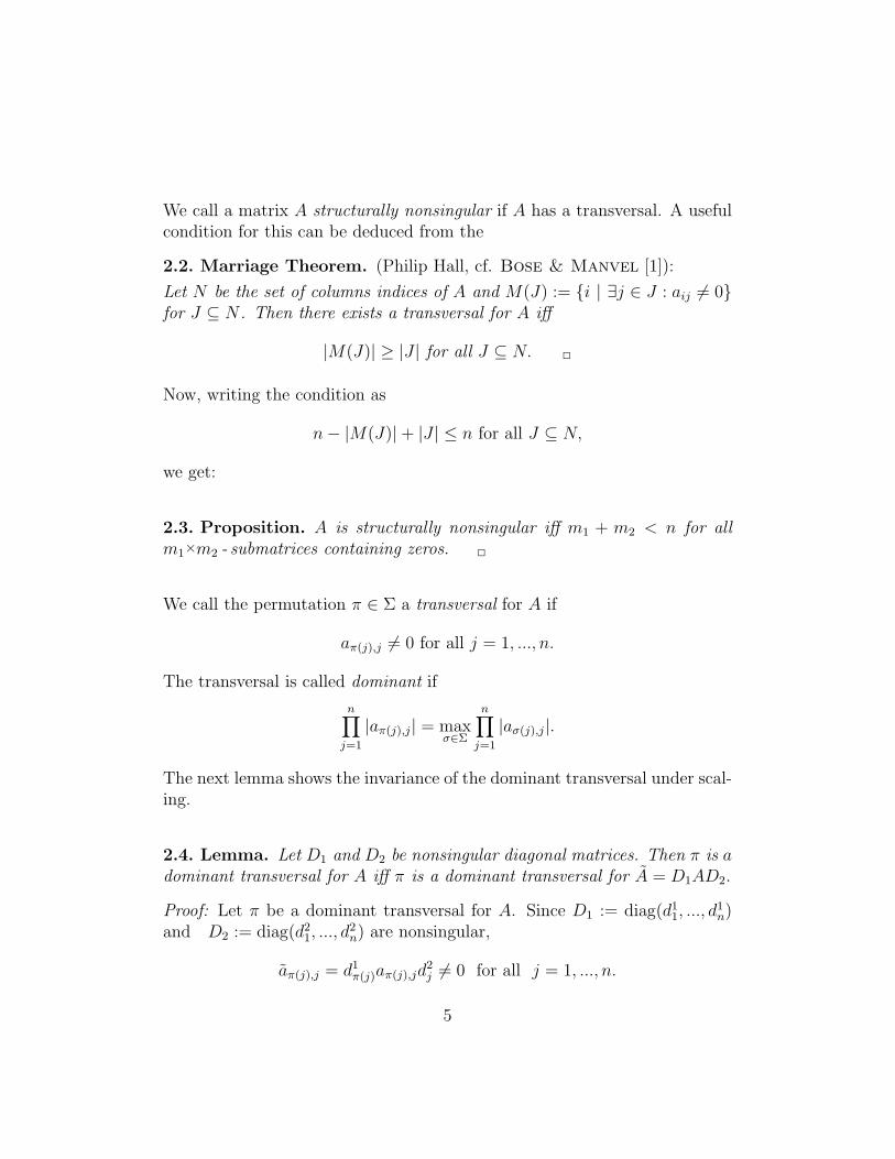
2.2. Marriage Theorem. (Philip Hall, cf. Bose & Manvel [1]):

Let N be the set of columns indices of A and M(J) := {i | ∃j ∈ J : aij 6= 0}for J ⊆ N . Then there exists a transversal for A iff

|M(J)| ≥ |J | for all J ⊆ N. ✷

Now, writing the condition as

n− |M(J)|+ |J | ≤ n for all J ⊆ N,

we get:

2.3. Proposition. A is structurally nonsingular iff m1 + m2 < n for allm1×m2 - submatrices containing zeros. ✷

We call the permutation π ∈ Σ a transversal for A if

aπ(j),j 6= 0 for all j = 1, ..., n.

The transversal is called dominant if

n∏

j=1

|aπ(j),j| = maxσ∈Σ

n∏

j=1

|aσ(j),j|.

The next lemma shows the invariance of the dominant transversal under scal-ing.

2.4. Lemma. Let D1 and D2 be nonsingular diagonal matrices. Then π is adominant transversal for A iff π is a dominant transversal for A = D1AD2.

Proof: Let π be a dominant transversal for A. Since D1 := diag(d11, ..., d1n)

and D2 := diag(d21, ..., d2n) are nonsingular,

aπ(j),j = d1π(j)aπ(j),jd2j 6= 0 for all j = 1, ..., n.

5

Given σ ∈ Σ, then, since τ and π are bijective,

n∏

j=1

|aσ(j),j|

|aπ(j),j|=

n∏

j=1

|d1σ(j)aσ(j),jd2j |

|d1π(j)aπ(j),jd2j |

=n∏

j=1

|aσ(j),j|

|aπ(j),j|≤ 1.

Since A = D−11 AD−1

2 , the converse direction holds, too. ✷

A n×n -matrix A is called an H-Matrix if

‖I −D1AD2‖∞ < 1 (1)

for suitable diagonal matrices D1 and D2. (The special case where one cantake for D2 the identity defines strictly diagonally dominant matrices.)

2.5. Theorem. For H-matrices and symmetric positive definite matrices,π = id is the unique dominant transversal.

Proof: (i) In (1), D1 and D2 are nonsingular matrices, because

|1− d1i aiid2i | ≤ |1− d1i aiid

2i |+

n∑

k=1k 6=i

|d1i aikd2k| < 1

implies d1i 6= 0, d2i 6= 0. According to Lemma 2.4 it only remains to showthat π = id is the unique dominant transversal for any matrix A = D1AD2

satisfying ‖I − A‖∞ < 1. But such an A is strongly diagonally dominant,hence this is true.

(ii) Let A be symmetric positive definite. Then

aii > 0 for i = 1, ..., n

since e(i)TAe(i) > 0 where e(i) is the ith unit vector in IRn. DefiningD1 = D2 = diag(a

−1/211 , ..., a−1/2

nn ), the matrix A = D1AD2 is still symmetricpositive definite with units on its diagonal. Again with Lemma 2.4 we mustonly show that id is dominant for A.

Let x(l,m) := e(l) + e(m) and

y(l,m) := e(l) − e(m) for l,m = 1, ..., n, l 6= m.

6

Thenx(l,m)T Ax(l,m) = all + alm + aml + amm

= 2(1 + alm) > 0

and similarlyy(l,m)T Ax(l,m) = 2(1− alm) > 0.

Thus|alm| < 1 for l,m = 1, ..., n, l 6= m,

so that any transversal π 6= id gives a product < 1 =∏

aii. ✷

2.6. Corollary. Permuting a matrix such that a dominant transversal is onthe diagonal restores a symmetric positive definite matrix, a strongly diago-nally dominant matrix, or an H-matrix from any permuted version of it.

We call a n×n -matrix A an I-matrix if

|aii| = 1 for i = 1, ..., n (2)

and|aij| ≤ 1 for i, j = 1, ..., n, i 6= j, (3)

and a strong I-matrix if (2) and

|aij| < 1 for i, j = 1, ..., n, i 6= j. (4)

It is clear that π = id is dominant for I-matrices and diagonally dominantmatrices. Moreover, when A is a strong I-matrix or strongly diagonally dom-inant then no other transversal can be dominant, too.

2.7. Example. Rice [12] described the difficulties to scale the matrix

A =

1 10+20 10+10 110+20 10+20 1 10+40

10+10 1 10+40 10+50

1 10+40 10+50 1

7

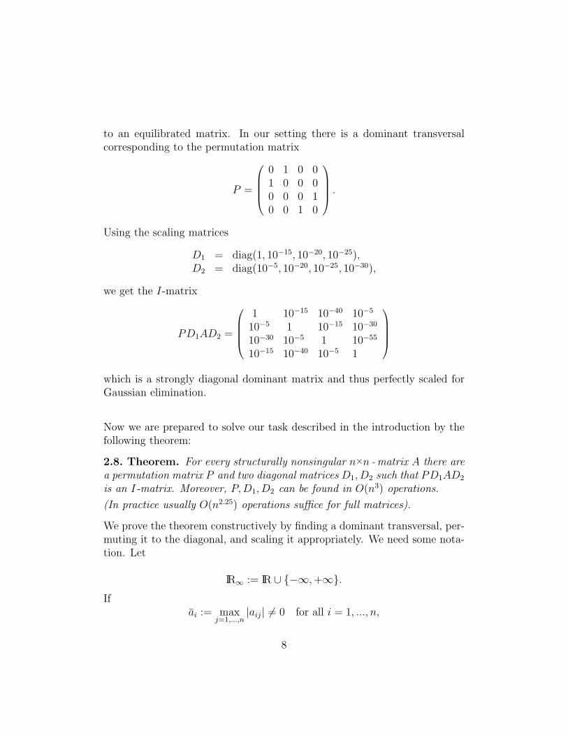
to an equilibrated matrix. In our setting there is a dominant transversalcorresponding to the permutation matrix

P =

0 1 0 01 0 0 00 0 0 10 0 1 0

.

Using the scaling matrices

D1 = diag(1, 10−15, 10−20, 10−25),D2 = diag(10−5, 10−20, 10−25, 10−30),

we get the I-matrix

PD1AD2 =

1 10−15 10−40 10−5

10−5 1 10−15 10−30

10−30 10−5 1 10−55

10−15 10−40 10−5 1

which is a strongly diagonal dominant matrix and thus perfectly scaled forGaussian elimination.

Now we are prepared to solve our task described in the introduction by thefollowing theorem:

2.8. Theorem. For every structurally nonsingular n×n -matrix A there area permutation matrix P and two diagonal matrices D1, D2 such that PD1AD2

is an I-matrix. Moreover, P,D1, D2 can be found in O(n3) operations.

(In practice usually O(n2.25) operations suffice for full matrices).

We prove the theorem constructively by finding a dominant transversal, per-muting it to the diagonal, and scaling it appropriately. We need some nota-tion. Let

IR∞ := IR ∪ {−∞,+∞}.

Ifai := max

j=1,...,n|aij| 6= 0 for all i = 1, ..., n,

8

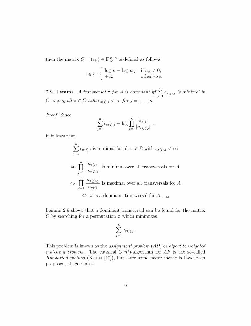
then the matrix C = (cij) ∈ IRn×n∞ is defined as follows:

cij :=

{

log ai − log |aij| if aij 6= 0,+∞ otherwise.

2.9. Lemma. A transversal π for A is dominant iffn∑

j=1cπ(j),j is minimal in

C among all π ∈ Σ with cπ(j),j < ∞ for j = 1, ..., n.

Proof: Sincen∑

j=1

cπ(j),j = logn∏

j=1

aπ(j)|aπ(j),j|

,

it follows that

n∑

j=1

cπ(j),j is minimal for all σ ∈ Σ with cσ(j),j < ∞

⇔n∏

j=1

aπ(j)|aπ(j),j|

is minimal over all transversals for A

⇔n∏

j=1

|aπ(j),j|

aπ(j)is maximal over all transversals for A

⇔ π is a dominant transversal for A. ✷

Lemma 2.9 shows that a dominant transversal can be found for the matrixC by searching for a permutation π which minimizes

n∑

j=1

cπ(j),j.

This problem is known as the assignment problem (AP ) or bipartite weightedmatching problem. The classical O(n3)-algorithm for AP is the so-calledHungarian method (Kuhn [10]), but later some faster methods have beenproposed, cf. Section 4.

9

Lemma 2.4 tells us in which cases there is no transversal for A. If there areonly zeros in one row i then the matrix C cannot be built because the maxi-mal row element ai does not exist. In the other cases the matching algorithmcannot compute an admissible permutation because for all σ ∈ Σ there is acolumn j with cσ(j),j = ∞. (In all these cases A is singular (Lemma 2.1)and therefore unsuitable for Gaussian elimination; so this does not restrictapplicability.)

Usually the assignment problem is formulated in graph theoretical terminol-ogy. Let G = (V1, V2, E) be a bipartite graph with V1 and V2 denoting thebipartition of the nodes. An edge e ∈ E will be written as an ordered pair(i, j) with i ∈ V1 and j ∈ V2. G is called complete (bipartite), if (i, j) ∈ Efor all i ∈ V1 and j ∈ V2. A matching (perfect matching) in G is a subsetM of the edges such that every node in V1 ∪ V2 is incident to at most one(exactly one) edge in M . Given weights cij ∈ IR for the edges (i, j) ∈ E wecan associate a weight

c(M) =∑

(i,j)∈M

cij

with every matching M . With G = (V1, V2, E), V1 = V2 = {1, ..., n} andE = {(i, j) | cij < ∞} the assignment problem is equivalent to the problemof finding a perfect matching with minimal weight.

It is well-known that the assignment problem can be written as the followinglinear program:

(LP) Find variables xij ∈ IR, i ∈ V1, j ∈ V2 minimizing

∑

(i,j)∈E

cijxij

under the conditions

∑

j∈V2(i,j)∈E

xij = 1 for i ∈ V1,

∑

j∈V1(i,j)∈E

xij = 1 for j ∈ V2,

10

∑

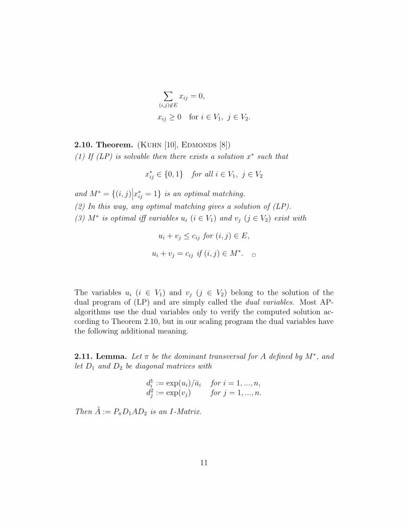
(i,j) 6∈E

xij = 0,

xij ≥ 0 for i ∈ V1, j ∈ V2.

2.10. Theorem. (Kuhn [10], Edmonds [8])

(1) If (LP) is solvable then there exists a solution x∗ such that

x∗ij ∈ {0, 1} for all i ∈ V1, j ∈ V2

and M∗ = {(i, j)∣

∣

∣x∗ij = 1} is an optimal matching.

(2) In this way, any optimal matching gives a solution of (LP).

(3) M∗ is optimal iff variables ui (i ∈ V1) and vj (j ∈ V2) exist with

ui + vj ≤ cij for (i, j) ∈ E,

ui + vj = cij if (i, j) ∈ M∗. ✷

The variables ui (i ∈ V1) and vj (j ∈ V2) belong to the solution of thedual program of (LP) and are simply called the dual variables. Most AP-algorithms use the dual variables only to verify the computed solution ac-cording to Theorem 2.10, but in our scaling program the dual variables havethe following additional meaning.

2.11. Lemma. Let π be the dominant transversal for A defined by M∗, andlet D1 and D2 be diagonal matrices with

d1i := exp(ui)/ai for i = 1, ..., n,d2j := exp(vj) for j = 1, ..., n.

Then A := PπD1AD2 is an I-Matrix.

11

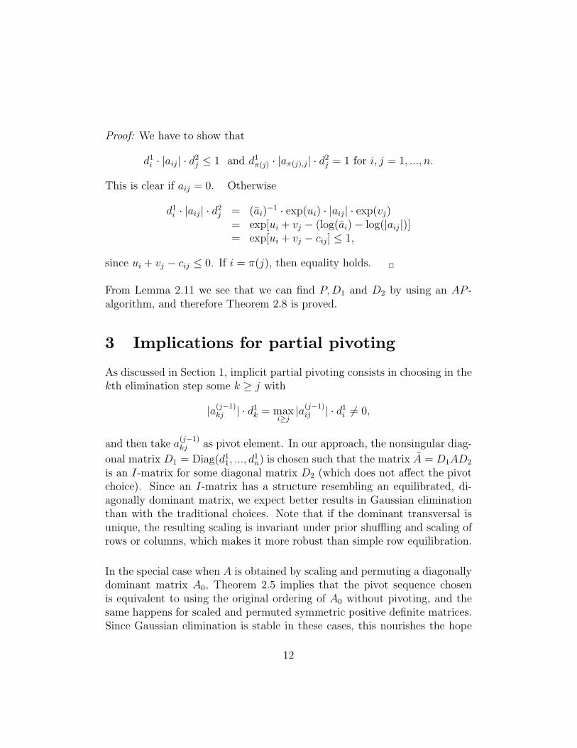
Proof: We have to show that

d1i · |aij| · d2j ≤ 1 and d1π(j) · |aπ(j),j| · d

2j = 1 for i, j = 1, ..., n.

This is clear if aij = 0. Otherwise

d1i · |aij| · d2j = (ai)

−1 · exp(ui) · |aij| · exp(vj)= exp[ui + vj − (log(ai)− log(|aij|)]= exp[ui + vj − cij] ≤ 1,

since ui + vj − cij ≤ 0. If i = π(j), then equality holds. ✷

From Lemma 2.11 we see that we can find P,D1 and D2 by using an AP -algorithm, and therefore Theorem 2.8 is proved.

3 Implications for partial pivoting

As discussed in Section 1, implicit partial pivoting consists in choosing in thekth elimination step some k ≥ j with

|a(j−1)kj | · d1k = max

i≥j|a

(j−1)ij | · d1i 6= 0,

and then take a(j−1)kj as pivot element. In our approach, the nonsingular diag-

onal matrix D1 = Diag(d11, ..., d1n) is chosen such that the matrix A = D1AD2

is an I-matrix for some diagonal matrix D2 (which does not affect the pivotchoice). Since an I-matrix has a structure resembling an equilibrated, di-agonally dominant matrix, we expect better results in Gaussian eliminationthan with the traditional choices. Note that if the dominant transversal isunique, the resulting scaling is invariant under prior shuffling and scaling ofrows or columns, which makes it more robust than simple row equilibration.

In the special case when A is obtained by scaling and permuting a diagonallydominant matrix A0, Theorem 2.5 implies that the pivot sequence chosenis equivalent to using the original ordering of A0 without pivoting, and thesame happens for scaled and permuted symmetric positive definite matrices.Since Gaussian elimination is stable in these cases, this nourishes the hope

12

that we also get a good pivoting sequence in the general situation.

The experimental results obtained in Section 4 indeed suggest that this holds,but we cannot prove this, since - unlike for H-matrices and symmetric pos-itive definite matrices - the I-matrix property is not preserved under elimi-nation. In particular, when using Gaussian elimination without pivoting onan I-matrix, it can happen that that a diagonal element becomes small (oreven zero) and hence is not suitable as pivot. Thus partial pivoting is stillessential. This is why, for general matrices, we do not use the transversal,but rather the associated left scaling matrix with implicit partial pivoting.This combines the best of both worlds. (The perfect, but expensive waywould be to restore I-dominance after each step; this would probably evenallow to prove strong stability statements - but we did not consider this indetail since it is not practical.)

When using the scaling factors computed with dual variables, a disadvantagebecomes apparent during triangularization when there are several elementsof absolute value 1 in a column of D1AD2. This always happens when hedominant transversal π is not unique. In this case, often elements not fromπ are taken as pivots, thus prematurely destroying the good ordering. Sincethe permuted matrix is generally no longer an I-matrix, one such occurencemay already imply that all later pivots are off the transversal, and the effec-tiveness of the scaling is much reduced.

Therefore we consider in the next section a method for improving the scalingfactors. Our goal will be the transformation to an I-dominant matrix A,defined as an I-matrix with a minimal number of off-diagonal elementsof absolute value 1 among all I-matrices D1AD2. (Note that in every I-matrix PπD1AD2 there are off-diagonal elements of absolute value 1 whenthe dominant transversal π for A is not unique.)

The main relevance of I-dominance is that it automatically finds a goodscaling, and preserves or restores good orderings in the cases where theorypredicts they are good. For sufficiently bad matrices, partial pivoting musttake care of the loss of I-dominance during elimination.

13

4 Practical Questions

For the choice of the AP-algorithm one has to consider not only runningtime and required work space, but also whether the program computes adual solution. We chose a version of the LSAPR-algorithm of Burkard

and Derigs [2] with starting procedure SAT3 of Carpaneto and Toth

[3]. In a timing test, this combination performed best among a number ofchoices tested, with an (experimental) running time of the order of O(n2.25)for full n×n -matrices. The key concept of the LSAPR-algorithm is the so-called shortest augmenting path method.

Let M be a matching in a graph G, then an M-alternating path P =(V (P ), E(P )) is a path in G the edges of which are alternately in M and notin M . Pi→j denotes an M -alternating path connecting the nodes i and j andPi→i denotes an M -alternating cycle. Pi→j is called an M-augmenting pathif the nodes i and j are not matched under M . Let P be an M -augmentingpath (M -alternating cycle). Then

M ⊕ P := (M \ E(P )) ∪ (E(P ) \M)

is again a matching, and

l(P ) := c(M ⊕ P )− c(M)

is called the length of P . A matching M is called extreme if it does not allowany M -alternating cycle P with l(P ) < 0. The SAP-method starts fromany extreme matching and successively augments along shortest augmentingpaths. For each of these matchings dual variables (u, v) ∈ IRV1∪V2 arecomputed with

ui + vj ≤ cij for (i, j) ∈ E,ui + vj = cij if (i, j) ∈ M.

Using the reduced cost coefficients

cij := cij − ui − vj > 0 for all edges (i, j) ∈ E,

the shortest augmenting path can be found similar to Dijkstra’s algorithmsince the reduced length of an alternating path P equals the sum

l(P ) =∑

(i,j)∈E(P )\M

cij

14

with nonnegative factors cij.

If the AP-program has finished with the optimal matching, the reduced costsdescribe the form of the I-matrix A = PπD1AD2 whereD1 andD2 are definedaccording to Lemma 2.11. Note that

cij > 0 ⇔ d1i · |aij| · d2j < 1 and

cij = 0 ⇔ d1i · |aij| · d2j = 1.

As in the elements of C, the value ∞ should be admitted for the scalingfactors. Then in the program ∞ is to be replaced by a suitable large numbersuch that values as ∞/2 or exp(±∞) are still defined, too.

We now consider a method for improving the scaling factors to get an I-dominant matrix A, as defined in Section 3.

4.1. Lemma. Assume that p ∈ IRn satisfies

cπ(j),k + pj − pk ≥ 0 for all j, k = 1, ..., n.

Thend1π(j) := exp(−(vj + pj))/|aπ(j),j| and

d2j := exp(vj + pj)

are scaling factors such that A = PπD1AD2 is an I-matrix. Moreover

cπ(j),k + pj − pk > 0 implies d1π(j)|aπ(j),k|d2k < 1.

Proof: Let |aπ(j),k| 6= 0 , then

d1π(j)|aπ(j),k|d2k = |aπ(j),j|

−1 · exp(−vj − pj) · |aπ(j),k| · exp(vk + pk)

= exp(cπ(j),j − vj − pj + cπ(j),k + vk + pk)= exp(−(cπ(j),k + pj − pk)) ≤ 1.

Equality holds only if cπ(j),k + pj − pk = 0. ✷

Now we shall show some ways for computing p ∈ IRn.

15

4.2. Algorithm. Equalization of the reduced costs cijin O(n2 · kmax) operationsp = 0

do k = 1, kmax

do j = 1, n

y1 = min{cπ(j),l + pj − pl∣

∣

∣ l = 1, ..., n, l 6= j}

y2 = min{cπ(l),j + pl − pj∣

∣

∣ l = 1, ..., n, l 6= j}

pj := pj + (y2 − y1)/2.

end do

end do

4.3. Theorem. Let D1 and D2 be diagonal matrices containing the scalingfactors via equalization with kmax ≥ [n/2] and let π be a unique dominanttransversal in A. Then A = PπD1AD2 is an I-dominant matrix.

For kmax = ∞ the algorithm maximizes

min{cπ(j),k + pj − pk∣

∣

∣ j 6= k}

and thus, if π is unique for A, we can regard the scaling factors via equaliza-tion with sufficiently large kmax as optimal scaling factors.

Unfortunately, equalization uses much running time. Computing scalingfactors computed from dual variables takes (in all our examples) signifi-cantly less time than the triangularization, but scaling via equalization withkmax = [n/2] costs on average 3 times as much as the factorization. So weconsider an alternative.

4.4. Theorem. (Path Selection)

Letrij := min l(Pi→j),

pj :=1

n

n∑

i=1i 6=π(j)

rij for i, j = 1, ..., n, i 6= π(j),

16

and let D1 and D2 be diagonal matrices containing the corresponding scalingfactors. Then A = PπD1AD2 is an I-dominant matrix.

Proof: We show that

cπ(j),k + pj − pk = 0 for j, k = 1, ..., n, j 6= k

iff (π(j), k) is an edge of an M-alternating cycle P of reduced length l(P ) = 0.

We note first that for all i, j, k = 1, ..., n, i 6= π(j), i 6= π(k), we have

rij + cπ(j),k ≥ min l(Pi→k) = rik,

cik ≥ min l(Pi→k) = rik.

Therefore

cπ(j),k + pj − pk

= cπ(j),k +1

n

∑

i=1i 6=π(j)

rij −1

n

∑

i=1i 6=π(k)

rik

=1

n

(

cπ(j),k + rπ(k),j + cπ(j),k − rπ(j),k +∑

i=1i 6=π(j),π(k)

(rij + cπ(j),k − rik))

≥1

n(cπ(j),k + rπ(k),j).

Hence

cπ(j),k + pj − pk

{

> 0 if (π(j), k) is an edge of a zero cycle,= 0 otherwise. ✷

Theoretically, rij can be computed by path selection of the SAP -methodinvolving O(n3) operations, but surely a more efficient implementation canbe found. However, this is not our aim, because here we only wanted todescribe the possibilities to vary the scaling program. Since there are manyAP -algorithms and new algorithms are still being proposed, we cannot yetdecide which method is the most appropriate matching strategy and whetherthere is a fast implementation to optimize the scaling factors by maximizing

min{cπ(j),k + pj − pk∣

∣

∣ j 6= k}.

It may even turn out feasible to update the matching after every eliminationstep and taking the entry of a dominant transversal in the ith column as ithpivot.

17

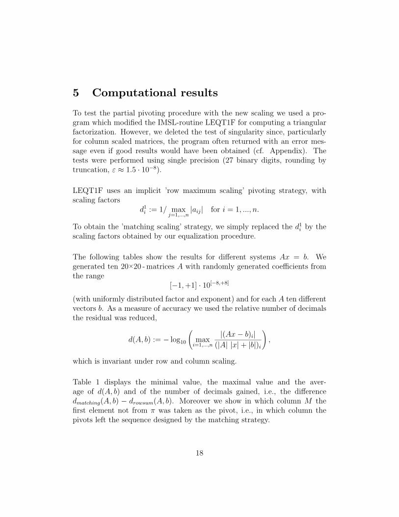
5 Computational results

To test the partial pivoting procedure with the new scaling we used a pro-gram which modified the IMSL-routine LEQT1F for computing a triangularfactorization. However, we deleted the test of singularity since, particularlyfor column scaled matrices, the program often returned with an error mes-sage even if good results would have been obtained (cf. Appendix). Thetests were performed using single precision (27 binary digits, rounding bytruncation, ε ≈ 1.5 · 10−8).

LEQT1F uses an implicit ’row maximum scaling’ pivoting strategy, withscaling factors

d1i := 1/ maxj=1,...,n

|aij| for i = 1, ..., n.

To obtain the ’matching scaling’ strategy, we simply replaced the d1i by thescaling factors obtained by our equalization procedure.

The following tables show the results for different systems Ax = b. Wegenerated ten 20×20 -matrices A with randomly generated coefficients fromthe range

[−1,+1] · 10[−8,+8]

(with uniformly distributed factor and exponent) and for each A ten differentvectors b. As a measure of accuracy we used the relative number of decimalsthe residual was reduced,

d(A, b) := − log10

(

maxi=1,...,n

|(Ax− b)i|

(|A| |x|+ |b|)i

)

,

which is invariant under row and column scaling.

Table 1 displays the minimal value, the maximal value and the aver-age of d(A, b) and of the number of decimals gained, i.e., the differencedmatching(A, b) − drowsum(A, b). Moreover we show in which column M thefirst element not from π was taken as the pivot, i.e., in which column thepivots left the sequence designed by the matching strategy.

18

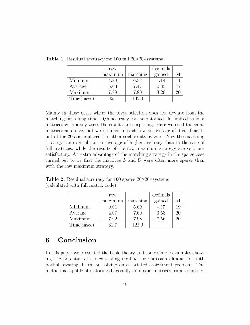
Table 1. Residual accuracy for 100 full 20×20 - systems

row decimalsmaximum matching gained M

Minimum 4.39 6.53 -.48 11Average 6.63 7.47 0.85 17Maximum 7.78 7.80 3.29 20Time(msec) 32.1 135.0

Mainly in those cases where the pivot selection does not deviate from thematching for a long time, high accuracy can be obtained. In limited tests ofmatrices with many zeros the results are surprising. Here we used the samematrices as above, but we retained in each row an average of 6 coefficientsout of the 20 and replaced the other coefficients by zero. Now the matchingstrategy can even obtain an average of higher accuracy than in the case offull matrices, while the results of the row maximum strategy are very un-satisfactory. An extra advantage of the matching strategy in the sparse caseturned out to be that the matrices L and U were often more sparse thanwith the row maximum strategy.

Table 2. Residual accuracy for 100 sparse 20×20 - systems(calculated with full matrix code)

row decimalsmaximum matching gained M

Minimum 0.01 5.69 -.27 19Average 4.07 7.60 3.53 20Maximum 7.92 7.98 7.56 20Time(msec) 31.7 122.0

6 Conclusion

In this paper we presented the basic theory and some simple examples show-ing the potential of a new scaling method for Gaussian elimination withpartial pivoting, based on solving an associated assignment problem. Themethod is capable of restoring diagonally dominant matrices from scrambled

19

and scaled versions of it, and it gives good scalings in the general case. How-ever, solving the assignment problem is in itself a nontrivial task, and forapplications to larger problems, further work must be done.

The timing results for the sparse matrices are of course not realistic sincewe used a full matrix implementation. While unweighted sparse assignmentproblems can be solved very fast, we do not know how fast the weightedsparse assignment problem can be solved, in particular since we need thedual solution as well. For some algorithms for solving sparse assignmentproblems see Derigs & Metz [7].

Another interesting possibility in the large scale case is the use of an in-complete factorization (without pivoting) of the I-matrix of Theorem 2.8, asa preconditioner for iterative methods for nonsymmetric linear systems likeQMR (Freund & Nachtigal [9]). In this case, equalization considera-tions play no longer a role, which speeds things up. Moreover, if a dominantmatching cannot be computed fast enough, one can probably design fastheuristics for finding a nearly dominant matching, which might suffice sincethe coefficients change anyway after each eliminiation step.

However, a proper treatment of these matters is beyond the scope of thepresent paper.

20

Appendix: Some remarks on published implementationsof Gaussian elimination

1. As remarked above, LEQT1F is sometimes far too cautious in assessingnonsingularity. Let the factorization routine LEQT1F take a

(j−1)ij as pivot

in the jth step of reduction and let

ω := |a(j−1)ij | · d1i .

LEQT1F gives failure if ω + n = n, and the program returns with an errormessage. This is appropriate when all elements of A are of the same orderunity, and the routine tries to achieve this by standard row equilibration. Butthis is not always good enough; for example LEQT1F stops with ω = 10−10

in the first step of reduction of the nonsingular matrix(

10−5 10+5

0 10+5

)

(which is already the upper triangular matrix U). We suggest just to give awarning if the test reports singularity and then to continue the reduction.

2. We also tested our scaling method on LINGL, a triangular factorizationprocedure developed byDekker [6]. Surprisingly, the resulting accuracy wasoften more than one decimal better. After inspection, the crucial differenceto LEQT1F turned out to be the accumulation of the inner products afterselecting the pivot and exchanging the rows.The accumulation of

Aii −∑

Lij ·Rji (5)

is done in LEQT1F by repeated subtraction and in LINGL according to

Aii −(

∑

Lij ·Rji

)

. (6)

By Wilkinson [14], Ch. I, (32.9/10), the rounding error in the computationof a1b1 + ...+ anbn by repeated addition is

(a1b1ε1 + ...+ anbnεn)(1 + ε)

where

|ε| ≤ 2−t, |ε1| <3

2n · 2−2t2 , |εr| <

3

2(n+ 2− r) · 2−2t2 ,

21

with t, t2 depending on the accuracy of the computer. This shows that per-muting a term of the summation from first position to last reduces its worstcase contribution to the total error by a factor n/2. Since in an I-matrix thediagonal terms are the largest terms in their rows, the pivots Aii tend to bethe largest element in the sum (5) and (6). This explains why the secondform (6) gives more accurate results.

In the mean time, IMSL changed the factorization routine, thus eliminatingthe weaknesses mentioned.

References

1. R. C. Bose; B. Manvel. Introduction to Combinatorial Theory. Wiley,Colorado State Univ. 1983.

2. R. E. Burkard; U. Derigs. Assignment and Matching Problems: SolutionMethods with FORTRAN-Programs. Lecture Notes in Econ. and Math.Systems, Springer, Berlin 1980.

3. G. Carpaneto; P. Toth. Solution of the assignment problem (Algorithm548). ACM Trans. Math. Softw. (1980), 104-111.

4. S. D. Conte and C. de Boor. Elementary Numerical Analysis. 3rd ed.,McGraw-Hill, Auckland 1981.

5. A. R. Curtis; J. K. Reid. On the automatic scaling of matrices forGaussian elimination. J. Inst. Math. Appl. 10 (1972), 118-124.

6. T. J. Dekker. ALGOL 60 Procedures in Numerical Algebra. Mathemat-ical Center Tracts 22 (1968), 20-21.

7. U. Derigs; A. Metz. An efficient labeling technique for solving sparseassignment problems. Computing 36 (1986), 301-311.

8. J. Edmonds. Maximum matching and a polyhedron with 0-1-vertices. J.Res. Nat. Bur. Stand. B69 (1965), 125-130.

22

9. R.W. Freund and N. M. Nachtigal. QMR: a quasi-minimal residualmethod for non-Hermitean linear systems. Numer. Math. 60 (1991), 315-339.

10. H. W. Kuhn. The Hungarian method for the assignment problem. NavalResearch Logistics Quarterly 2 (1955) 83.

11. B. N. Parlett; T. L. Landis. Methods for scaling to double stochasticform. Linear Algebra Appl. 48 (1982), 53-79.

12. J. R. Rice. Matrix Computation and Mathematical Software. McGraw-Hill, New York 1981.

13. J. H. Wilkinson. Error Analysis of Direct Methods of Matrix Inversion.J. Assoc. Comput. Mach. 8 (1961).

14. J. H. Wilkinson. Rounding Errors in Algebraic Processes. Prentice Hall,Englewood Cliffs, N.J. 1963.

23