1822 ieee transactions on automatic control,...

1822 IEEE TRANSACTIONS ON AUTOMATIC CONTROL, VOL. 55, NO. 8, AUGUST 2010

Multiple Model Adaptive Control With MixingMatthew Kuipers and Petros Ioannou, Fellow, IEEE

Abstract—Despite the remarkable theoretical accomplishmentsand successful applications of adaptive control, the field is not suf-ficiently mature to solve challenging control problems where strictperformance and robustness guarantees are required. Critical tothe design of practical control systems for these challenging ap-plications, and currently lacking in parameter estimation-basedadaptive control schemes, is an approach that explicitly accountsfor robust-performance and stability specifications. Towards thisgoal, this paper describes a robust adaptive control approach calledadaptive mixing control that makes available the full suite of pow-erful design tools from LTI theory, e.g., mixed- synthesis. Thestability and robustness properties of adaptive mixing control areanalyzed. It is shown that the mean-square regulation error is ofthe order of the modeling error provided the unmodeled dynamicssatisfy a norm-bound condition. And when the parameter estimateconverges to its true value, which is guaranteed if a persistenceof excitation condition is satisfied, the adaptive closed-loop systemconverges exponentially fast to a closed-loop system comprising theplant and some LTI controller that satisfies the control objective.A benchmark example is presented, which is used to compare theadaptive mixing controller with other adaptive schemes.

Index Terms—Multiple model adaptive control, robust adaptivecontrol.

I. INTRODUCTION

W HEN model uncertainties are sufficiently small, modernlinear time invariant (LTI) control theories, e.g., and

-synthesis [1]–[3], ensure, when possible, satisfactory closed-loop objectives specified in meaningful engineering terms (fre-quency weights on the relevant transfer functions) are met. How-ever, changes in operating conditions, failure or degradation ofcomponents, or unexpected changes in system dynamics may allviolate the assumption of small uncertainty, particularly para-metric uncertainty. The impact of such “large” uncertainty is thata single fixed LTI controller may no longer achieve satisfactoryclosed-loop behavior, let alone stability. What is needed is a con-troller that is able to monitor the plant dynamics in order to adjustits control law to compensate for such parametric uncertainty andother modeling errors [4, Sec. 1.3].

Adaptive control copes with large parametric uncertainty bytuning controller gains in response to estimated changes in themodel. Since in conventional (robust) adaptive control [4], [5]the controller gains are calculated in real time based on theestimated plant model, the complicated relationship between

Manuscript received May 06, 20098 December, 2009; revised November 10,2009; accepted December 08, 2009. First published February 05, 2010; currentversion published July 30, 2010. This work was supported by the National Sci-ence Foundation under Grant 0510921. Recommended by Associate Editor A.Astolfi.

The authors are with the Department of Electrical Engineering, University ofSouthern California, Los Angeles, CA 90024 USA (e-mail: [email protected];[email protected]).

Digital Object Identifier 10.1109/TAC.2010.2042345

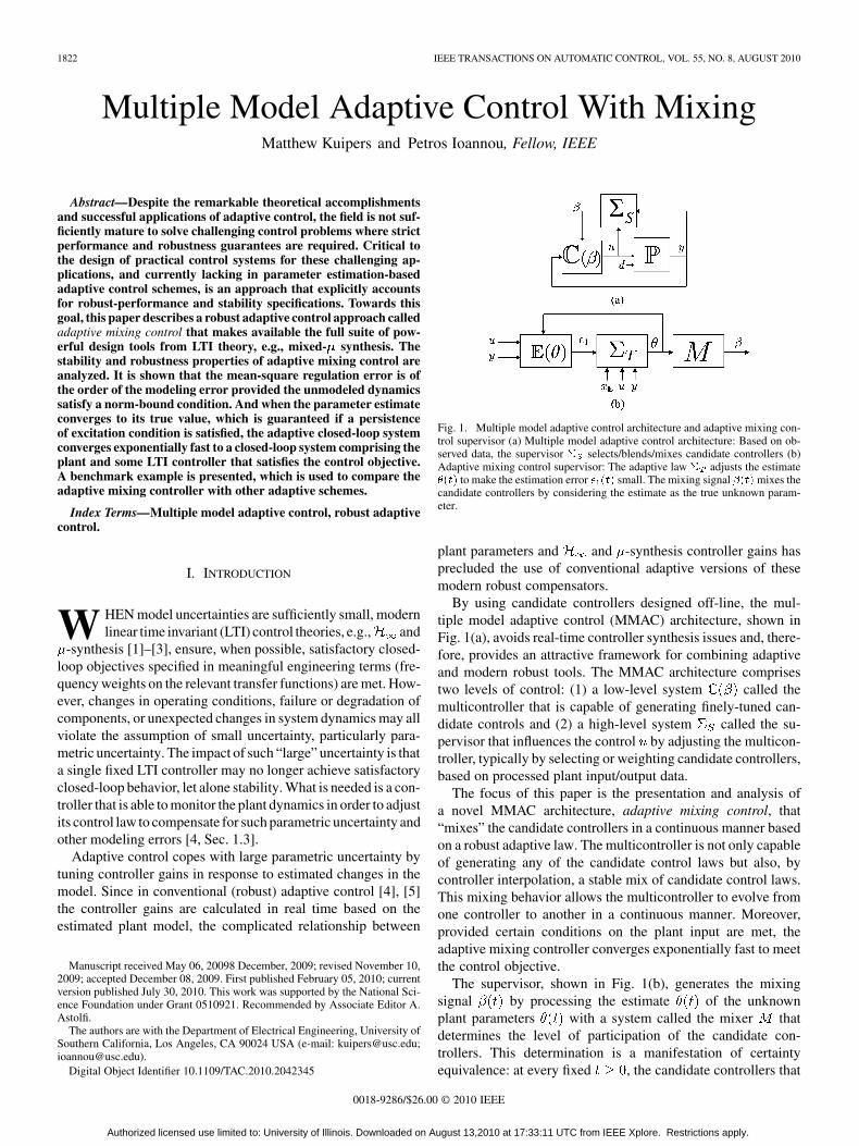
Fig. 1. Multiple model adaptive control architecture and adaptive mixing con-trol supervisor (a) Multiple model adaptive control architecture: Based on ob-served data, the supervisor � selects/blends/mixes candidate controllers (b)Adaptive mixing control supervisor: The adaptive law � adjusts the estimate�� to make the estimation error � �� small. The mixing signal �� mixes thecandidate controllers by considering the estimate as the true unknown param-eter.

plant parameters and and -synthesis controller gains hasprecluded the use of conventional adaptive versions of thesemodern robust compensators.

By using candidate controllers designed off-line, the mul-tiple model adaptive control (MMAC) architecture, shown inFig. 1(a), avoids real-time controller synthesis issues and, there-fore, provides an attractive framework for combining adaptiveand modern robust tools. The MMAC architecture comprisestwo levels of control: (1) a low-level system called themulticontroller that is capable of generating finely-tuned can-didate controls and (2) a high-level system called the su-pervisor that influences the control by adjusting the multicon-troller, typically by selecting or weighting candidate controllers,based on processed plant input/output data.

The focus of this paper is the presentation and analysis ofa novel MMAC architecture, adaptive mixing control, that“mixes” the candidate controllers in a continuous manner basedon a robust adaptive law. The multicontroller is not only capableof generating any of the candidate control laws but also, bycontroller interpolation, a stable mix of candidate control laws.This mixing behavior allows the multicontroller to evolve fromone controller to another in a continuous manner. Moreover,provided certain conditions on the plant input are met, theadaptive mixing controller converges exponentially fast to meetthe control objective.

The supervisor, shown in Fig. 1(b), generates the mixingsignal by processing the estimate of the unknownplant parameters with a system called the mixer thatdetermines the level of participation of the candidate con-trollers. This determination is a manifestation of certaintyequivalence: at every fixed , the candidate controllers that

0018-9286/$26.00 © 2010 IEEE

Authorized licensed use limited to: University of Illinois. Downloaded on August 13,2010 at 17:33:11 UTC from IEEE Xplore. Restrictions apply.

KUIPERS AND IOANNOU: MULTIPLE MODEL ADAPTIVE CONTROL WITH MIXING 1823

were designed for are mixed such that closed-loopobjectives are met.

The MMAC concept is not new and has been around for quitesome time. One recent approach is the so-called supervisorycontrol [6]–[8], in which controller selection is made by contin-uously comparing in real time suitably defined norm-squaredestimation errors, also referred to as performance signals, andthe candidate controller associated with the smallest perfor-mance signal is placed in the loop according to an appropriateswitching logic. Following the idea of supervisory control,logic-based switching and multiple models were combinedwith conventional adaptive control [9]–[11] with the objectiveof improving transient performance of conventional adaptiveschemes. Also incorporating logic-based switching is theso-called unfalsified control approach [12], [13], which is anonidentifier-based deterministic approach. The unfalsifiedcontrol approach is a model free approach and differs frommost other switching schemes. It relies on measured data toselect the right controller. Even though the method guaranteesconvergence to a stabilizing robust controller, the simulationstudies in [14], [15] report unacceptable transients. This is con-sistent with intuition: at the outset, measured input-output datamay largely reflect initial conditions, resulting in the selectionof a poorly performing controller for an extended period oftime until measurement quality improves. Therefore the claimin [12], [13] that no knowledge of the plant model or its formis required is true for stability but not for performance unlessfurther modifications are added as discussed in [15].

Switching-based schemes have a number of advantages.Switching in adaptive control was originally introduced asa method to overcome the loss of stabilizability in param-eter estimation based adaptive control [16], [17]. Also, theseschemes have the advantage of rapid adaptation to large, abruptparameter changes. This is a desirable switching behavior.Switching, however, may exhibit undesirable behaviors thatcould negatively affect performance. Explained heuristically, ifhysteresis is used and the true model is near the boundary oftwo candidate models, the supervisor may persistently select acontroller that does not achieve desirable closed-loop behavior,despite observed data indicating an acceptable candidate con-troller is preferred. To encourage switching, the hysteresisconstant may be reduced or replaced with a dwell-time logic,but at the increased risk of long-term intermittent switchingbetween multiple controllers, resulting in transients from im-proper initialization of the new controller1.

Another promising MMAC approach is based on theso-called robust MMAC (RMMAC) methodology that pro-vides guidelines for designing both the candidate controller set(using mixed- synthesis tools) and the supervisor [18]–[20].The RMMAC approach originated from the multiple modeladaptive estimation/MMAC methods [21] of the 1970s, ofwhich there have been numerous successful applications basedon adaptations of these methods [22]–[24]. The RMMACsupervisor is based on a dynamic hypothesis testing schemethat generates for each candidate the posterior probability that

1State resetting schemes may reduce transients after switching. Adaptivemixing control is presented as an alternative approach that aims to avoidstate-resetting due to unnecessary switching.

its model is “closest” to the true plant. These probabilities areused to weight the candidate controller outputs, or, as done inthe RMMAC/S variant, to switch into the loop the candidatecontroller associated with the highest posterior probability.Given accurate disturbance and noise models that satisfy thestandard Kalman filter assumptions, simulations demonstraterapid adaptation and superior performance compared to anonadaptive mixed- compensator [20]. Acknowledged withinthe same reference, however, is that special care is needed tocompensate for an inaccurate stochastic disturbance model.The RMMAC/XI architecture was proposed to handle a rangeof disturbance powers, at the cost of additional Kalman filters.Still, if the disturbance power is significantly outside the ex-pected range, poor performance may occur. And although lossof stabilizability is not an issue (because there is no estimatedmodel), it should be noted that no stability results have beenpublished.

The immediate motivation of adaptive mixing control is toprovide an adaptive control approach that is capable of incorpo-rating the full suite of powerful LTI tools, while avoiding someof the performance issues associated with undesirable switchingphenomena and an unknown or uncertain disturbance model,offering an alternative to the existing MMAC approaches forparticular applications. The unique feature of adaptive mixingcontrol with respect to existing MMAC approaches, includingRMMAC, is that the intent is not to converge to one controller,but rather a stable mix of candidate controllers. This mixing be-havior avoids switching and, in turn, some of its undesirable be-haviors. Also, while an adaptive mixing control scheme’s per-formance may be improved by incorporating a priori knowl-edge of the disturbance, the evaluations in Section VI and [25],where the latter focuses on a multiple estimator variant of the ap-proach presented in this paper, demonstrate that adaptive mixingcan achieve satisfactory performance despite significant pertur-bations in the disturbance power and bandwidth. Last, utilizingpre-computed controllers, adaptive mixing control avoids com-putational and existence issues of calculating controller gainswhen stabilizability of the estimated plant is lost.

NOTATION AND PRELIMINARIES

Suppose that is a matrix. The transpose of isdenoted by . For a -vector , is the Euclidean norm

and the corresponding induced matrix norm of isdenoted as . If is a function of time, then the normof is denoted as and the truncated norm is defined

as , where is a

constant, provided that the integral exists. By we meanthat with , and we say that if exists.Let , and consider the set

for a given constant , where are some finite con-stants, and is independent of . We say that is -small in



the mean square sense (m.s.s.) if . Furthermore, con-sider the signal and the set

where are some finite constants. We say that is-small in the m.s.s. if .Let and be the transfer function and impulse

response, respectively, of some LTI system. If is aproper transfer function and analytic in forsome , where denotes the real part of , thenthe system norm is given by .The system norm of is defined as

. The induced

system norm of is given by . Ifand then .

If , denotes the boundary of the set , anddenotes the set-theoreticdifference. An openball of radius

centered around point is denoted as. Throughout, denotes the

standard basis vector, i.e., the component of is one; all othercomponents are zero. The function denotes thebump function if ; otherwise,

. The function is smooth and supported on .We say that a square, bounded, piece-wise continuous is

exponentially stable (e.s.) if its transition matrix satisfiesfor some forall .

Theorem 1: Let be compact and be any con-stant in and . If the parameterized detectablepair is continuously differentiable with respectto , where and , thenthere exists a continuously differentiable matrix function

, such that1) if for all and , then the equilibrium

of is e.s.2) if for all and for some constant

, then there exists a such that ifthe equilibrium of is e.s.

where .The proof of Theorem 1 is a combination of the well-known

results of [26] and the linear time varying (LTV) stability resultsfound in [5, Theorem 3.4.11]. We would like to emphasize thatthe existence of the observer gain of Theorem 1 is utilizedonly for analysis purposes, not design. Furthermore, an explicitdefinition of is not required.

II. A SIMPLE EXAMPLE

In this section, we use a simple example to introduce the adap-tive mixing control approach in a tutorial manner. Consider theuncertain plant

(1)

where is an unknown constant that belongs to the knowninterval ; is a bounded disturbance, i.e.,

; and is a multiplicative plant uncertainty. isassumed to be a proper rational transfer function that is analyticin for some known . We refer to

as the nominal model. The control objective is toplace the pole of the closed-loop nominal plant in the interval

; guarantee that and are bounded; and when ,guarantee and converge to zero as .

We consider control laws of the form , whereis to be chosen such that the control objective is met for any

. The question is whether a single fixed valueof will meet the control objective given that is unknownexcept that it belongs to the interval . If we applythe above control law to the plant (1), we obtain the closed-loopsystem

(2)

When , the closed-loop pole of (2) is , andit follows from the bound that a single fixedvalue of cannot meet the control objective.

Let us assume that the large parametric uncertaintyis divided into the three smaller subintervals

called parameter subsets, so that the control objective could bemet if it is known which parameter subset contains . Let usalso assume that the following three fixed controllers (candidatecontrollers) are used based on which parameter subset contains

:

(3)

(4)

(5)

If is known a priori then the control objective of placing thenominal closed-loop pole in the interval is met by se-lecting the appropriate candidate control law from (3)–(5) basedon which parameter subset contains . If belongs to morethan one parameter subset, then any of the appropriate candidatecontrol laws may be chosen. Furthermore, overall closed-loopstability is guaranteed if

The right hand side of the above takes on its minimum value overwhen and . Thus, a sufficient

condition for stability is .If is not known a priori but is measured or estimated on-

line, a strategy is needed for constructing a control law thatmeets the control objective based on the real-time knowledge of

. Our objective is to design a control law fromthe candidate control laws (3)–(5) continuous in to avoid dis-continuities in the control signal that may occur as a result ofnoise or if the measured value of varies across parameter sub-sets. Discontinuities in the control signal are a practical concern



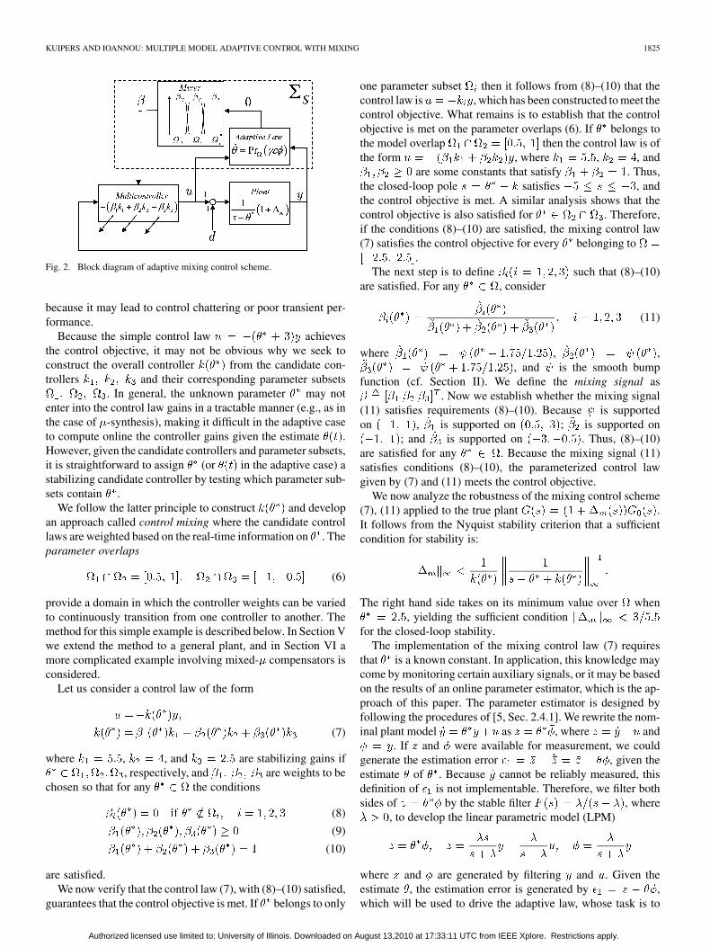
Fig. 2. Block diagram of adaptive mixing control scheme.

because it may lead to control chattering or poor transient per-formance.

Because the simple control law achievesthe control objective, it may not be obvious why we seek toconstruct the overall controller from the candidate con-trollers and their corresponding parameter subsets

. In general, the unknown parameter may notenter into the control law gains in a tractable manner (e.g., as inthe case of -synthesis), making it difficult in the adaptive caseto compute online the controller gains given the estimate .However, given the candidate controllers and parameter subsets,it is straightforward to assign (or in the adaptive case) astabilizing candidate controller by testing which parameter sub-sets contain .

We follow the latter principle to construct and developan approach called control mixing where the candidate controllaws are weighted based on the real-time information on . Theparameter overlaps

(6)

provide a domain in which the controller weights can be variedto continuously transition from one controller to another. Themethod for this simple example is described below. In Section Vwe extend the method to a general plant, and in Section VI amore complicated example involving mixed- compensators isconsidered.

Let us consider a control law of the form

(7)

where , , and are stabilizing gains if, respectively, and are weights to be

chosen so that for any the conditions

(8)

(9)

(10)

are satisfied.We now verify that the control law (7), with (8)–(10) satisfied,

guarantees that the control objective is met. If belongs to only

one parameter subset then it follows from (8)–(10) that thecontrol law is , which has been constructed to meet thecontrol objective. What remains is to establish that the controlobjective is met on the parameter overlaps (6). If belongs tothe model overlap then the control law is ofthe form , where , , and

are some constants that satisfy . Thus,the closed-loop pole satisfies , andthe control objective is met. A similar analysis shows that thecontrol objective is also satisfied for . Therefore,if the conditions (8)–(10) are satisfied, the mixing control law(7) satisfies the control objective for every belonging to

.The next step is to define such that (8)–(10)

are satisfied. For any , consider

(11)

where , ,, and is the smooth bump

function (cf. Section II). We define the mixing signal as. Now we establish whether the mixing signal

(11) satisfies requirements (8)–(10). Because is supportedon , is supported on ; is supported on

; and is supported on . Thus, (8)–(10)are satisfied for any . Because the mixing signal (11)satisfies conditions (8)–(10), the parameterized control lawgiven by (7) and (11) meets the control objective.

We now analyze the robustness of the mixing control scheme(7), (11) applied to the true plant .It follows from the Nyquist stability criterion that a sufficientcondition for stability is:

The right hand side takes on its minimum value over when, yielding the sufficient condition

for the closed-loop stability.The implementation of the mixing control law (7) requires

that is a known constant. In application, this knowledge maycome by monitoring certain auxiliary signals, or it may be basedon the results of an online parameter estimator, which is the ap-proach of this paper. The parameter estimator is designed byfollowing the procedures of [5, Sec. 2.4.1]. We rewrite the nom-inal plant model as , where and

. If and were available for measurement, we couldgenerate the estimation error , given theestimate of . Because cannot be reliably measured, thisdefinition of is not implementable. Therefore, we filter bothsides of by the stable filter , where

, to develop the linear parametric model (LPM)

where and are generated by filtering and . Given theestimate , the estimation error is generated by ,which will be used to drive the adaptive law, whose task is to



Fig. 3. Simulation results. (a) Plant output: Adaptive mixing control (solid); Adaptive pole placement control (dashed). (b) Estimate �� of � � ��: Adaptivemixing control (solid); Adaptive pole placement control (dashed).

tune to make “small.” This LPM can be used to generate awide-class of adaptive laws for generating the estimate of[5, Section 8.5], and we choose the adaptive law as the gradientalgorithm with projection modification

otherwise(12)

where is the adaptive gain and is the projection op-erator that restricts to . We refer to as theunnormalized estimation error to distinguish it from the nor-malized estimation error . Completing the adaptivemixing control design, we combine the adaptive law (12) with

by replacing with its estimate , and the adaptivemixing control scheme is shown in Fig. 2.

A. Simulation

For simulation purposes, we use the plant parameters, , , and

. Additionally, sensor noise is simu-lated by substituting the noisy measurementfor in the control law and parameter estimator. We use the con-trol parameters , , , and , whichwere chosen by trial and error. For comparison, we also simulatean adaptive pole placement control (APPC) scheme that usesan identical parameter estimator as the adaptive mixing controlscheme. The APPC scheme differs from the adaptive mixingcontrol scheme only in the control law, where the APPC schemereplaces the mixing control law (7) with the APPC control

. Moreover, the desired pole location of theAPPC control law was chosen from robustness considerations.The plant output is shown in Fig. 3(a). In this example, boththe adaptive mixing control and APPC schemes regulate theplant output towards a neighborhood of zero, where the adap-tive mixing scheme has slightly faster convergence. Simulationsshow that the APPC scheme remains stable for ; adap-tive mixing control remains stable for ; and perfectidentification remains stable for . Adaptive

mixing control’s mild improvement in performance and robust-ness is because oscillations in (shown in Fig. 3(b)) caused bythe modeling error terms , , and do not affect thecontrol law when . This is not the case in APPC; thus,oscillations in caused by further excite . Because bothschemes use an adaptive law with projection modification, theonline estimates remain bounded by , whichtogether with the large model uncertainty gives rise to the “saw-tooth” shaped trajectories shown in Fig. 3(b).

III. GENERAL PROBLEM FORMULATION

Consider the SISO LTI plant

(13)

(14)

(15)

where represents the nominal plant; the vectorcontains the unknown parameters of

; ; is the measuredvalue of corrupted by the bounded sensor noise , i.e.,

; is an unknown multiplicative perturbation;and is a bounded disturbance, i.e., ; Thecontrol objective is to choose the plant input so that the plantoutput is regulated close to zero. We make the following as-sumptions on the plant to meet the control objective:

P1. is a monic polynomial whose degree isknown.P2. Degree .P3. is proper, rational, and analytic in

for some known .P4. for some known compact convex set

.Consider the state-space realization of (13)

(16)

We make the additional assumption to make control meaningful:P5. The pairs and are detectableand stabilizable, respectively, on .



It should be emphasized that both unstable and nonminimumphase plants are admissible despite requirements P1-P5.

Given is a family of candidate controllers ,where are rational transfer functions anddenotes the index set , and the parameter partition

, where each parameter subset is com-pact and covers , i.e., . The candidate controllerset and parameter partition has been developed such that forevery and each , the control lawyields a stable closed-loop system that meets some performancerequirements. If contains and the control is chosen as

, then a sufficient condition for stability overis

(17)

Let and be the boundaries of the sets and , respec-tively. To facilitate control mixing, the partition has an overlap-ping property: for all and any there existconstants and such that . The param-eter overlaps set is the set of all points that belong tomore than one parameter subset. The candidate controllers andparameter subsets can, for example, be generated by the methodof [19], modified to generate overlapping parameter subsets.

Remark 1: A conventional adaptive controller could be in-cluded in the candidate controller set to account for the case

. This is the topic of future work.Remark 2: As in many MMAC approaches, the complexity

of the controller design increases with the number of candidatecontrollers, which may result in an impractical design. A prioriknowledge can be used to decrease the number of unknown pa-rameters and size of , and, in turn, decrease the number ofcandidate controllers.

1) The Problem: The objective of this paper is to propose aprovably correct MMAC scheme which is capable of achieving1) global boundedness of all system signals and 2) regulation ofall plant signals in the absence of unmodeled dynamics, distur-bances, and sensor noise.

A deterministic approach is pursued because the disturbanceis only known to be bounded. The unknown parameter vectors

enter the plant model linearly and the plant remains de-tectable and stabilizable on . Therefore, in order to side-stepissues associated with discontinuous switching among candi-date controllers, we present a deterministic MMAC approachthat tunes the multicontroller in a continuous manner based onthe estimate of .

IV. CONCEPTUAL FRAMEWORK

The adaptive mixing control architecture comprises two sys-tems: the multicontroller and the robust adaptive super-visor , which in turn consists of a robust parameter estimatorand mixer . For notational simplicity, the following defini-tions are made. If (for some ), then is said tobe an active parameter subset. denotes the index set of allactive parameter subsets at , i.e., .We define the set of all admissible mixing values at as

. The set of all admissible mixing values is denotedby .

A. Multicontroller

The multicontroller , constructed from , is a dynam-ical system capable of generating a mix of candidate controllaws. The multicontroller is given by the stabilizableand detectable state-space realization

(18)

where is the multicontroller state vector; thesystem matrices , , are of compatible dimensions;and the mixing signal and estimateis generated by the supervisor and tunes . For fixed valuesof and , the multicontrollerhas the transfer function

(19)

(20)

The multicontroller satisfies three properties:C1. The elements of , , andare continuously differentiable in and .C2. , where and is

standard basis vector.C3. For all and any ,internally stabilizes the plant.

Property C1 ensures that the closed-loop system varies slowly ifand are tuned slowly. Property C2 allows for each candidate

controller to be recovered. Property C3 ensures that is astabilizing certainty equivalence control law for any admissiblemixing signal, independent of the mixer implementation. Themulticontroller can be viewed as a generalization of the multi-controller used in supervisory control [6].

Construction of the multicontroller involves interpolating thecandidate controllers over the parameter overlaps . Numerouscontroller interpolation approaches have been proposed in thecontext of gain scheduling. These methods interpolate controllerpoles, zeros, and gains [27]; solutions of the Riccati equationsfor an design [28]; state-space coefficient matrices of bal-anced controller realizations [29]; state and observer gains [30];controller output [31]–[33], i.e., , where

. As in gain scheduling, these interpolation methodsmay not satisfy the point-wise stability requirement C3 (cf. thecounter examples of [34], [35]). Thus, if one of these interpola-tion methods is used then property C3 should be verified.

Fortunately, there also exist theoretically justified methods[34]–[36], which can be used to construct the multicontroller.The following result is adapted from [34]:

Lemma 2: Consider the nominal plant givenby (14) and the stable coprime factorization

that dependson smoothly. Let the stable transfer functions ,

, , and depend on smoothly and



satisfy the double Bezout identity (omitting dependencies onand )

Suppose , where is some compact set, andare stabilizing negative feedback con-

trollers for any . Let each controller be given astable coprime factorization , and wedefine

(21)

(22)

(23)

for . If the controller is given by

(24)where , ,and are some positive constants that satisfy

, then is stabilizing and iffor and for .

Motivated by Lemma 2, consider the multicontroller

(25)

(26)

(27)

where , , and are given by (21)–(23), respectively, andthe function denotes a smooth projection func-tion2: is continuously differentiable and if

. The function is used to ensure that each is onlyevaluated on and, therefore, stable; otherwise, may gen-erate an unbounded out-of-the-loop signal if and .

We now examine if this multicontroller satisfies propertiesC1-C3. Property C1 follows immediately by inspection of thefilters of Lemma 2 that define the multicontrollerand because is smooth. Let us now consider property C3.For fixed constants and , we have for

, and for . Thus

(28)

2� is not the same as the projection operator �� used in the adaptivelaw. � can be constructed, for example, from smooth bump functions �.

Fig. 4. Multicontroller implementation and robust performance formulation (a)Multicontroller structure (b) General control configuration.

Because indexes only stabilizing controllers, it followsfrom Lemma 2 that internally stabilizes theplant, satisfying C3. Moreover, if for some ,

, and C2 is satisfied. Fig. 4(a) shows animplementation of the multicontroller that avoids unboundedout-of-the-loop signals [37].

By Q-blending we mean the multicontroller scheme (25),which is given in a multiple input-multiple output (MIMO)format to emphasize that this approach is suitable for extensionsof adaptive mixing control to the MIMO case.

We now consider robust performance as the control objective,which is formulated in the standard general control configura-tion shown in Fig. 4(b), as the control objective. Motivated towork with a normalized uncertainty, we model the multiplica-tive uncertainty as , where the knownstable transfer function serves as a frequency depen-dent weight and is any stable transfer function satisfying

. The transfer matrix is assumed to con-tain the plant and its interconnection with the per-formance and uncertainty weights that describe the control ob-jective; is the exogenous input (for example, say

), and is the exogenous output. The ma-trix transfer function is formed by absorbing thecontroller into as shown in Fig. 4(b). We say that a con-troller yields robust performance if is stableand satisfies , wheresatisfies ; is a stable transfer matrix; and

denotes . Let us assume that eachcandidate yields robust performance for all . Asdemonstrated by the following result, a Q-blending multicon-troller preserves robust performance.

Lemma 3: If the multicontroller is given by (25)and, for some generalized plant and , the candi-date controller yields robust performance for all ,then for all and the multicontrolleryields robust performance with respect to .

Proof: The transfer matrix has the form(cf. [2, pp. 150]), where . For any

and , it follows that ,for , and for . Thus



and, consequently, is stable and.

Remark 3: The choice of controller interpolation scheme af-fects the complexity of the multicontroller. Say, for example,that the candidate controller orders are . An inter-polation approach that schedules the controller gains with re-spect to will result in a multicontroller order of .The output-blending scheme results in a multi-controller order of . To analyze the Q-blending schemeshown in Fig. 4(a), let us assume that the orders of andare . Then the order of the Q-blending multicontroller is

. The a priori theoretical properties of theQ-blending approach should be carefully weighed against itscomplexity.

B. Robust Adaptive Supervisor

The robust adaptive supervisor, shown in Fig. 1(b), is a dy-namical system that takes as input the measured plant signals

and outputs the mixing signals that “config-ures” the multicontroller . Note that, because we are im-plementing the supervisor, the multicontroller may access thestates of the supervisor, including the parameter estimate .

The mixer implements the mapping . Thefollowing properties of are assumed

M1. is continuously differentiable.M2.

Property M1, together with C1 ensures that if is tuned slowlythen the closed-loop system will vary slowly. M2, together withC3, ensures that is a certainty equivalence stabilizingcontroller, i.e., for any the controller meetsthe control objective. Thus, if the control lawis applied to the nominal plant (14), the closed-loop system isinternally stable, and the closed-loop characteristic polynomial

is Hurwitz. Further-more, when this control law is applied to the overall plant (13),the closed-loop system is stable if

(29)

If satisfies C3, the design of the mixer is indepen-dent of ; otherwise, one must ensure, for all , that

meets the control objectives. Assuming require-ment C3 is satisfied, the designer has considerable freedom inconstructing , and one such approach, as in Section III and inthe sequal, is to define based on the smooth bump functiongiven in Section II.

Because is unknown, cannot be calculatedand, therefore, cannot be implemented. Thus, the adaptivemixing control approach replaces with its estimate . Thewell known counter example of Rohrs et al., [38] demonstratesthat for even small modeling errors that an adaptive systemmay become unstable. Thus, because of the presence of mul-tiplicative uncertainty , disturbance , and sensor noise ,we use a robust online parameter estimator to regain as muchof the robustness of the known case as possible.

The robust parameter estimator comprises an error modeland a robust adaptive law , also referred to as the tuner.

The error model is constructed by selecting an appropriate

parameterization of the plant model. We proceed with the de-sign of the error model by constructing a LPM using the sametechnique as in Section III. The interested reader is referred to[5, Sec. 2.4.1] for a detailed description. The LPM of the nom-inal system (14) is given by , where

(30)

(31)

(32)

where is a design constant and is a proper stableminimum-phase filter. The estimation error is generated byregarding as the true parameter , i.e.,

. We define the error model as the dynamical systemwhose inputs are the observed data and , and its output is

. The error model is realized from (30)–(32) and has theform

(33)

(34)

(35)

where is Hurwitz and is tuned by . Notethat is affine in .

When the error model is connected to the true plantin the presence of the multiplicative perturbation andbounded disturbance and noise , is given by ,where

(36)

is the modeling error term and acts as an estimation disturbance.The filter can be chosen to mitigate the deleterious effectsof on estimation. For this purpose, will typically havea bandpass frequency response to filter out signal bias and dis-turbances at low frequencies and sensor noise and unmodeleddynamics at high frequencies. For simplicity, we chooseto be analytic in .

The robust adaptive law can be implemented by a wide-class of algorithms [5, Chapter 8.5] whose dynamics take thefairly general form

(37)

(38)

(39)

where is the adaptive law’s state;is an auxiliary state required by the tuning algorithm; and

is the dynamic component of the normalization signalthat guarantees that . We choose

and to be implemented with projection modification [4], [5]in order to constrain to . The adaptive law is imple-mented by any of the algorithms found in [4], [5] with projectionmodification that guarantees

E1. , if , , or

E2. , ifE3.



where is the normalized estimation error. Addition-ally, we assume that the robust adaptive law satisfies

E4.i.e., adaptation ceases when . This assumption is satisfiedby all adaptive laws of [4], [5] except those with -modification.

Remark 4: If the plant parameters enter the model in a non-linear fashion, one can often overparameterize the plant model.Overparameterization increases the class of admissible plants;thus, there may be some loss of performance, and, as in theexample of [6, Sec. X], plant models that are not stabilizablemay be introduced. Because the controller gains are computedoff-line, adaptive mixing control avoids the computational andexistence issues that arise in conventional adaptive control whenstabilizability is lost. Furthermore, the adaptive law can be mod-ified to ensure that does not remain in a specified neighbor-hood about the points that lead to a loss of stabilizability (cf. 7.6of [5]).

Remark 5: We believe that there will be no significant diffi-culties in extending adaptive mixing control to the MIMO case,which is currently under investigation.

C. Stability and Robustness Results

We now summarize the main results.Theorem 4: Let the unknown plant be given by (13) and

satisfying the plant assumptions P1-P5. Consider the adaptivemixing controller with the multicontroller given by(18) and satisfying assumptions C1-C3; error model givenby (33)–(35); robust adaptive law given by (37)–(39) andsatisfying assumptions E1-E4; and mixer satisfying M1-M2.

1) If then as , where. Furthermore, let the multicontroller

be given by the Q-blending scheme (25), and for somegeneralized plant and let the candidatecontroller yield robust performance for all . If

, then as, where is the solution to

(40)

and the triplet is the state-space realizationof some controller that yields robust performance with re-spect to the generalized plant .

2) There exists such that if , whereand is a finite constant, then the adap-

tive mixing control scheme guarantees that. Furthermore, there exist constants such that

(41)

where .The proof is given in the Appendix . In result 1), exponentialconvergence of estimate to the true value can be guaran-teed provided is persistently exciting (PE). The control inputcan be augmented with an auxiliary signal that forcesto be sufficiently rich of order , guaranteeing is PE if theplant is controllable and observable. For output tracking of con-trollable, observable plants, the reference signal may naturallyensure that is PE; otherwise, guaranteeing that is PE can be

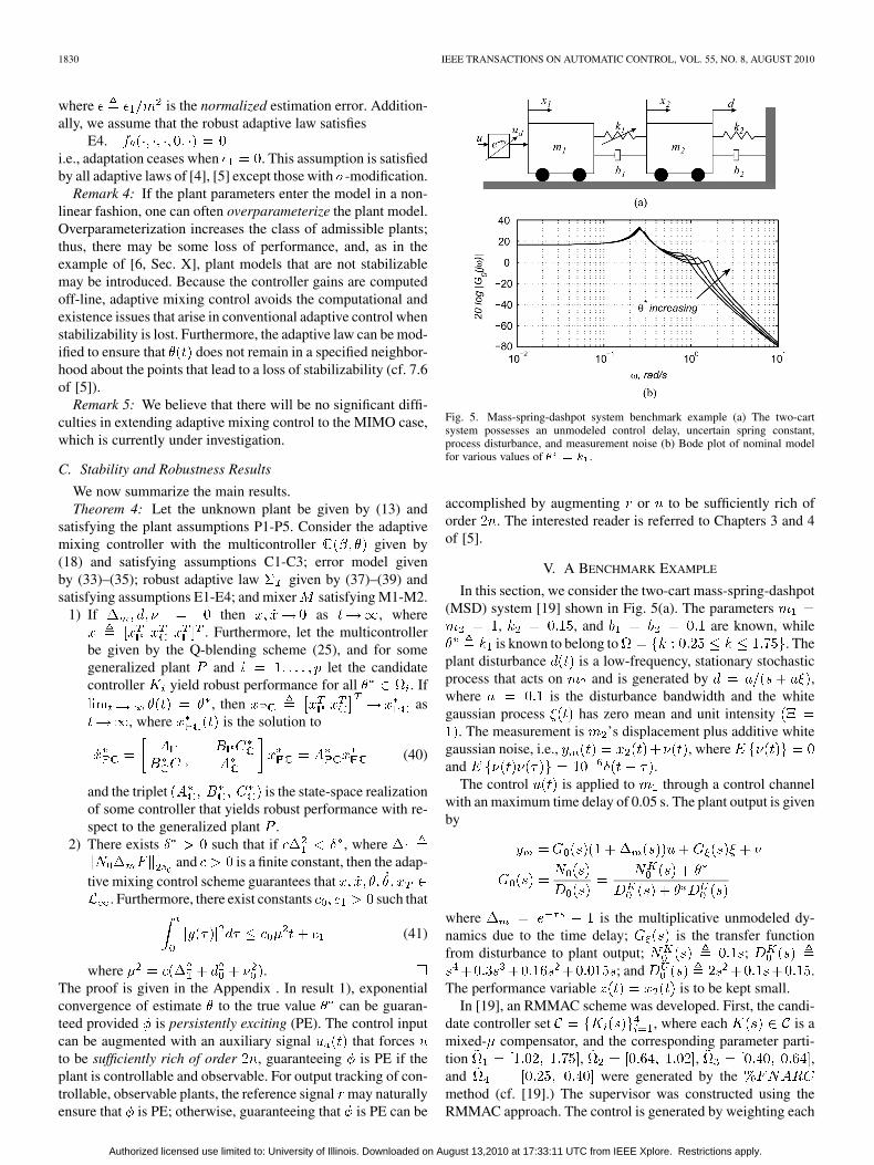
Fig. 5. Mass-spring-dashpot system benchmark example (a) The two-cartsystem possesses an unmodeled control delay, uncertain spring constant,process disturbance, and measurement noise (b) Bode plot of nominal modelfor various values of � � � .

accomplished by augmenting or to be sufficiently rich oforder . The interested reader is referred to Chapters 3 and 4of [5].

V. A BENCHMARK EXAMPLE

In this section, we consider the two-cart mass-spring-dashpot(MSD) system [19] shown in Fig. 5(a). The parameters

, , and are known, whileis known to belong to . The

plant disturbance is a low-frequency, stationary stochasticprocess that acts on and is generated by ,where is the disturbance bandwidth and the whitegaussian process has zero mean and unit intensity

. The measurement is ’s displacement plus additive whitegaussian noise, i.e., , whereand .

The control is applied to through a control channelwith an maximum time delay of 0.05 s. The plant output is givenby

where is the multiplicative unmodeled dy-namics due to the time delay; is the transfer functionfrom disturbance to plant output; ;

; and .The performance variable is to be kept small.

In [19], an RMMAC scheme was developed. First, the candi-date controller set , where each is amixed- compensator, and the corresponding parameter parti-tion , , ,and were generated by themethod (cf. [19].) The supervisor was constructed using theRMMAC approach. The control is generated by weighting each



controller output by the output of the supervisor, i.e.,.

For a fair comparison, the adaptive mixing control and su-pervisory control schemes utilize the candidate controller setdeveloped in the RMMAC design. Let us now consider the de-sign of an adaptive mixing control scheme. We start the designof the multicontroller by enlarging each parameter subset

so that mixing regions are artificially introduced. After ex-panding the boundaries of , , by 10%, we have thenew parameter partition , ,

, and . The multicon-troller design is completed by performing output blending, i.e.,

. It is clear that requirements C1 andC2 are satisfied. Using standard mixed- analysis tools, we havefound property C3 holds over . Also, for comparison, an adap-tive mixing control scheme was developed using the Q-blendingapproach to construct the multicontroller.

The design of the mixing system is accomplished bydefining the functions , , as

where is the smooth bump function. The mixing signalis generated by normalizing , i.e.,

, and requirements M1 and M2 are satisfied.The final component of the adaptive mixing control scheme

is the robust adaptive law. The LPM isused to derive the adaptive law, where

(42)

(43)

(44)

is the modeling error; is the bandpass filter

where and . The passbandis , with a peak-to-peak 0.25 dB ripple;and the stopband is , with a at-tenuation level. These values were chosen to make use of thefrequency range that is largely affected by , as shown graph-ically in Fig. 5(b), while filtering out the remaining frequenciesthat may become dominated by .

An adaptive law using the gradient method based on integralcost is used:

ififotherwise

TABLE IMODEL ASSUMPTIONS SATISFIED

where is the estimate of and is thedynamic normalization signal, where

The design parameters of the adaptive law were chosen by trialand error.

The supervisory adaptive control scheme (labeled as SAC inTable I and the figures) is constructed by monitoring the es-timation error signals for ,where each constant is chosen as the center of the interval

, and and are generated by (42) and (43), respec-tively. Note that the filters that generate and are iden-tical to the filters in the adaptive mixing control scheme. Thus,any effect attributed to the filter is experienced by bothschemes. The supervisory scheme generates the monitoring sig-nals , and selects thecontroller corresponding to the smallest monitoring signal sub-ject to a hysteresis logic. Hysteresis logic prohibits switchingunless the smallest monitoring signal is at least 0.1% smallerthan the currently selected monitoring signal. The value of thehysteresis constant was chosen by trial and error based on an ac-ceptable compromise between rapid response and reduced like-lihood of switching due to noise and modeling error.

Fig. 6 shows the results of two different adaptive mixing con-trollers: an output blending scheme and a Q-blending scheme.The output-blending scheme exhibits better transient and long-term performance compared to the Q-blending mixing scheme,which is more susceptible to bursting-type behaviors becausethe Q-blending multicontroller depends on both and .This makes it more susceptible to variations.

Based on the above results, we chose to use the adaptivemixing control scheme with output blending to compare withthe RMMAC and supervisory adaptive control schemes. Al-though an extensive evaluation of the adaptive mixing control,



Fig. 6. Comparison of the plant outputs of the Q-blending and output-blendingschemes with � � ��, � � ��, and nominal disturbance model.

RMMAC, and supervisory schemes are beyond the scope of thispaper3, we present some simulation results that illustrate someof the potential benefits of the adaptive mixing control scheme.Table I presents short-term and long-term

output RMS values for various values of ,and with and all model assumptions satisfied. The re-sults of Table I are the average of five trials.

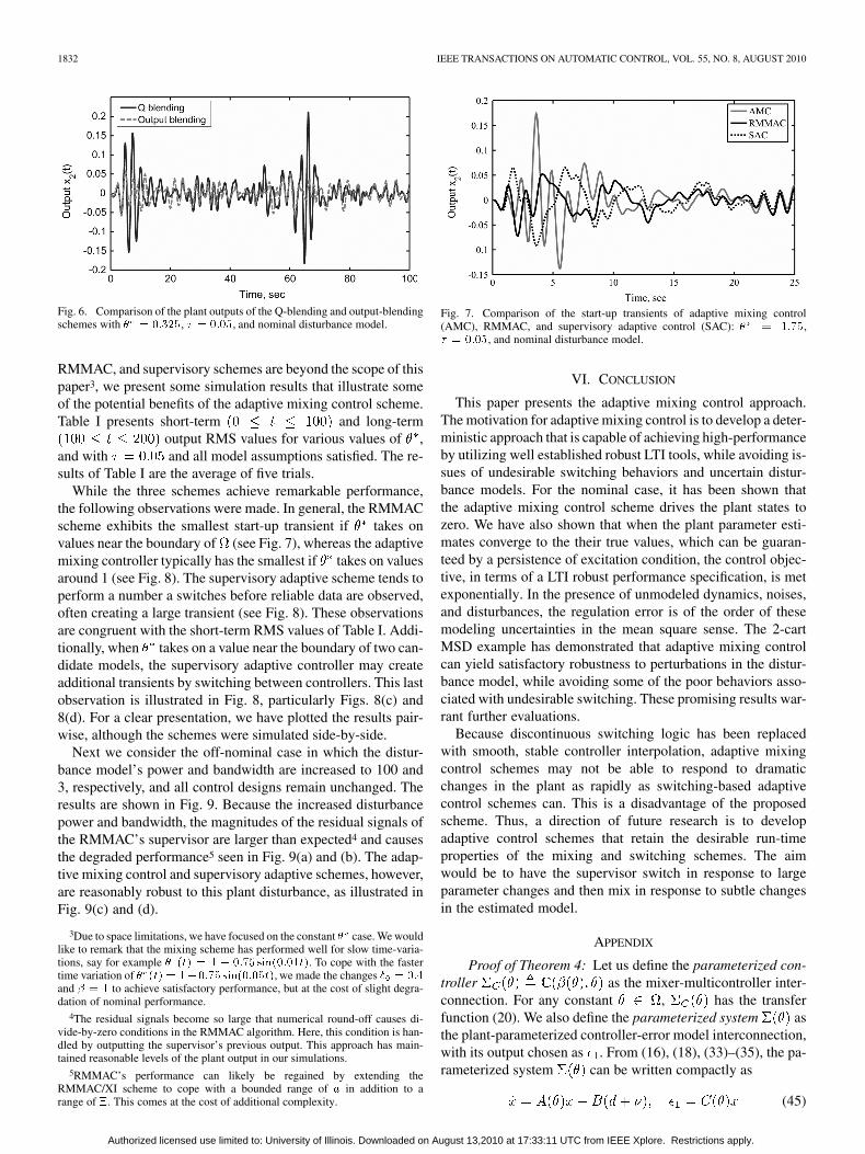
While the three schemes achieve remarkable performance,the following observations were made. In general, the RMMACscheme exhibits the smallest start-up transient if takes onvalues near the boundary of (see Fig. 7), whereas the adaptivemixing controller typically has the smallest if takes on valuesaround 1 (see Fig. 8). The supervisory adaptive scheme tends toperform a number a switches before reliable data are observed,often creating a large transient (see Fig. 8). These observationsare congruent with the short-term RMS values of Table I. Addi-tionally, when takes on a value near the boundary of two can-didate models, the supervisory adaptive controller may createadditional transients by switching between controllers. This lastobservation is illustrated in Fig. 8, particularly Figs. 8(c) and8(d). For a clear presentation, we have plotted the results pair-wise, although the schemes were simulated side-by-side.

Next we consider the off-nominal case in which the distur-bance model’s power and bandwidth are increased to 100 and3, respectively, and all control designs remain unchanged. Theresults are shown in Fig. 9. Because the increased disturbancepower and bandwidth, the magnitudes of the residual signals ofthe RMMAC’s supervisor are larger than expected4 and causesthe degraded performance5 seen in Fig. 9(a) and (b). The adap-tive mixing control and supervisory adaptive schemes, however,are reasonably robust to this plant disturbance, as illustrated inFig. 9(c) and (d).

3Due to space limitations, we have focused on the constant � case. We wouldlike to remark that the mixing scheme has performed well for slow time-varia-tions, say for example � �� . To cope with the fastertime variation of � �� , we made the changes � � �� and � � � to achieve satisfactory performance, but at the cost of slight degra-dation of nominal performance.

4The residual signals become so large that numerical round-off causes di-vide-by-zero conditions in the RMMAC algorithm. Here, this condition is han-dled by outputting the supervisor’s previous output. This approach has main-tained reasonable levels of the plant output in our simulations.

5RMMAC’s performance can likely be regained by extending theRMMAC/XI scheme to cope with a bounded range of � in addition to arange of �. This comes at the cost of additional complexity.

Fig. 7. Comparison of the start-up transients of adaptive mixing control(AMC), RMMAC, and supervisory adaptive control (SAC): � � ��,� � ��, and nominal disturbance model.

VI. CONCLUSION

This paper presents the adaptive mixing control approach.The motivation for adaptive mixing control is to develop a deter-ministic approach that is capable of achieving high-performanceby utilizing well established robust LTI tools, while avoiding is-sues of undesirable switching behaviors and uncertain distur-bance models. For the nominal case, it has been shown thatthe adaptive mixing control scheme drives the plant states tozero. We have also shown that when the plant parameter esti-mates converge to the their true values, which can be guaran-teed by a persistence of excitation condition, the control objec-tive, in terms of a LTI robust performance specification, is metexponentially. In the presence of unmodeled dynamics, noises,and disturbances, the regulation error is of the order of thesemodeling uncertainties in the mean square sense. The 2-cartMSD example has demonstrated that adaptive mixing controlcan yield satisfactory robustness to perturbations in the distur-bance model, while avoiding some of the poor behaviors asso-ciated with undesirable switching. These promising results war-rant further evaluations.

Because discontinuous switching logic has been replacedwith smooth, stable controller interpolation, adaptive mixingcontrol schemes may not be able to respond to dramaticchanges in the plant as rapidly as switching-based adaptivecontrol schemes can. This is a disadvantage of the proposedscheme. Thus, a direction of future research is to developadaptive control schemes that retain the desirable run-timeproperties of the mixing and switching schemes. The aimwould be to have the supervisor switch in response to largeparameter changes and then mix in response to subtle changesin the estimated model.

APPENDIX

Proof of Theorem 4: Let us define the parameterized con-troller as the mixer-multicontroller inter-connection. For any constant , has the transferfunction (20). We also define the parameterized system asthe plant-parameterized controller-error model interconnection,with its output chosen as . From (16), (18), (33)–(35), the pa-rameterized system can be written compactly as

(45)



Fig. 8. Simulation results with � � ��, � � ��, and nominal disturbance model: Adaptive mixing control (AMC), RMMAC, and supervisory adaptivecontrol (SAC) (a) Plant output: AMC and RMMAC (b) Controller weights: AMC and RMMAC (c) Plant output: AMC and SAC (d) Controller weights: AMC andSAC.

where and the triplet is de-fined in the obvious manner. The closed-loop adaptive system

is formed by replacing the parameter of the pa-rameterized system with the tuned estimates generatedby the robust adaptive law . The closed-loop system (45)is in a form suitable for analysis using the tunability approachof [39]. Also, it has been establish in [40] that along the tra-jectories of there exists a unique global solution

, .Step 1: Establish that for all fixed , is a

detectable pair.Consider the adaptive law initialization ,

where is any fixed constant in . The vectorsrepresent the initial estimates of the coefficients of the

and , respectively. Let , , and .Thus, it follows that and, because , there is noadaptation, i.e., . Therefore the closed-loop system is anLTI system. Since , we have . Thus, it followsfrom (30) and (31) that the signals and satisfy

(46)

Similarly, the parameterized controller is an LTI systemand and also satisfy

(47)

From (46) and (47), and satisfy

The characteristic equation of the above system is

Since is a stable minimum phase filter andis Hur-

witz by properties C3 and M2, we have thatas . From the detectability of and

, together with the conver-gence of and to zero, it follows that as

. Since is a stability matrix, the convergence ofand to zero implies that as . Therefore,

because it has been shown that converges to zero forall when , the parameterized pair

is detectable on .Step 2: Establish that along the solutions of there

exists a function such thatis exponentially stable.

Recall that the robust adaptive law guarantees that , ,. Applying [5, Lemma 3.3.2] to (36), together with

and , yields

(48)

(49)



Fig. 9. Simulation results with � � ��, � � ��, and the off-nominal disturbance model with a disturbance power of �� and a bandwidth of ��

�: Adaptive mixing control (AMC), RMMAC, and supervisory adaptive control (SAC) (a) Plant output: AMC and RMMAC (b) Controller weights: AMC andRMMAC (c) Plant output: AMC and SAC (d) Controller weights: AMC and SAC.

and since and , it followsthat . Therefore, , , , where

and is some constant.Because properties C1 and M1 guarantee that and

, respectively, are continuously differentiable, the parame-terized controller is continuously differentiable with respectto . The error model is affine in and, therefore, con-tinuously differentiable. Consequently, the pairis continuously differentiable with respect to . Furthermore,because the adaptive law guarantees that and

, it follows from the detectability result of Step 1 and re-sult 2) of Theorem 1 that there exists a continuously differen-tiable function such that

is e.s. provided that for some .For large , i.e., large or , this condition may not besatisfied even for small . By using the lengthy analysis ap-proach of [5, Section 9.9.1], involving a contradiction argu-ment, boundedness of the closed-loop signals can be provenprovided satisfies a bound condition that is independent of

. However, for simplicity, we continue with an alternativeanalysis approach, where we assume the filter is chosenso that is sufficiently small, say , so that for

, the inequality is always satisfied. There-fore, is e.s., i.e., the transition matrix ofsatisfies for some positive constants

and . Note that if , the adap-tive law guarantees that , and from result 1) of The-orem 1, is e.s. Since is continuous and is compact,

, where is a slight abuse of notation and is takento mean .

Step 3: Establish boundedness and convergence ofLet , where , and denotes

any finite constant. Recall that is defined in (39).By applying output injection, we rewrite (45) as

(50)

where in Step 2 we established e.s. of the homogeneous part of(50).

We establish that : By Lemma 3.3.3 of [5] and thee.s. property of , we have that

(51)

where because is a continuous function of time.Applying the norm to and

, where is bounded (a consequence of thecontinuously differentiability of and the compact-ness of ), yields

(52)

(53)

where the second inequalities of (52) and (53) were obtained byfirst recognizing that and are subvectors of and thenapplying inequality (51). Consider the fictitious normalizationsignal . Note that because ,it follows from the definitions of and that .



Substituting (52), (53), and into the definition ofyields

(54)

where the second inequality is obtained by using .From the definition of it follows that:

(55)

Applying the Bellman-Gronwall Lemma (cf. [5, Lemma 3.3.9])

to (55) yields the inequality

, where . Let us assumethat is chosen such that . Becauseimplies , it follows that for

, we have . Since , we have that, and together with (property E1)

implies that . Moreover, it followsthat because , which, together withproperty E3, implies .

We now turn our attention to the injected system (50). Re-call that is e.s., and are bounded, and is in

. Therefore, , and, in turn, . Nowwe examine the mean-square properties of . From [5, Corollary3.3.3] it follows that and, in turn, since

is a subvector of . Thus, (41) holds. To summarize, the con-dition for stability is , for someconstants and , where isthe bound for such that is e.s.

Let us consider that . For this case,is a function because and(from E2 and ). Thus, since is e.s., we have

, , and as . From theconvergence of , and consequently , it follows from (50)that as .

We now consider the case that . It followsfrom (16) and (18) that:

(56)

(57)

where and is tuned by the adaptivelaw. Let . From Lemma 3, the triplet

is the state space realization of a controllerthat yields robust performance for the generalized plant . From(40) and (57), the dynamics of is given by

. Becauseis Hurwitz and , we have .Therefore, as .

REFERENCES

[1] P. M. Young, “Controller design with mixed uncertainties,” in Proc.Amer. Control Conf., Baltimore, MD, Jun. 1994, pp. 2333–2337.

[2] S. Skogestad and I. Postlethwaite, Multivariable Feedback Control:Analysis and Design, 2nd ed. New York: Wiley-Interscience, 2005.

[3] K. Zhou and J. C. Doyle, Essentials of Robust Control. EnglewoodCliffs, NJ: Prentice Hall, 1997.

[4] P. A. Ioannou and B. Fidan, Adaptive Control Tutorial, ser. Advancesin Design and Control. Philadelphia, PA: SIAM, 2006.

[5] P. A. Ioannou and J. Sun, Robust Adaptive Control. Upper SaddleRiver, NJ: Prentice-Hall, 1996.

[6] A. S. Morse, “Supervisory control of linear set-point controllers—Part1: Exact matching,” IEEE Trans. Autom. Control, vol. 41, no. 10, pp.1413–1431, Oct. 1996.

[7] A. S. Morse, “Supervisory control of linear set-point controllers—Part2: Robustness,” IEEE Trans. Autom. Control, vol. 42, no. 11, pp.1500–1515, Nov. 1997.

[8] J. Hespanha, D. Liberzon, A. S. Morse, B. D. O. Anderson, T. S. Brins-mead, and F. De Bruyne, “Multiple model adaptive control. Part 2:Switching,” Int. J. Robust Nonlin. Control, vol. 11, no. 5, pp. 479–496,Apr. 2001.

[9] K. S. Narendra and J. Balakrishnan, “Improving transient response ofadaptive control systems using multiple models and switching,” IEEETrans. Autom. Control, vol. 39, no. 9, pp. 1861–1866, Sep. 1994.

[10] K. S. Narendra and C. Xiang, “Adaptive control of discrete-time sys-tems using multiple models,” IEEE Trans. Autom. Control, vol. 45, no.9, pp. 1669–1686, Sep. 2000.

[11] A. Karimi and I. D. Landau, “Robust adaptive control of a flexibletransmission system using multiple models,” IEEE Trans. Control Syst.Technol., vol. 8, no. 2, pp. 321–331, Mar. 2000.

[12] M. Safonov and T.-C. Tsao, “The unfalsified control concept andlearning,” IEEE Trans. Autom. Control, vol. 42, no. 6, pp. 843–847,Jun. 1997.

[13] M. Stefanovic, R. Wang, and M. Safonov, “Stability and convergencein adaptive systems,” in Proc. Amer. Control Conf., Boston, MA, 2004,pp. 2012–2021.

[14] A. Dehghani, B. D. O. Anderson, and A. Lanzon, “Unfalsified adaptivecontrol: A new controller implementation and some remarks,” in Proc.Eur. Control Conf., Jul. 2007, pp. 709–716.

[15] S. Baldi, G. Battistelli, E. Mosca, and P. Tesi, “Multi-model unfalsifiedadaptive switching supervisory control,” Automatica, vol. 46, no. 2, pp.249–259, Feb. 2010.

[16] A. S. Morse, D. Q. Mayne, and G. C. Goodwin, “Applications of hys-teresis switching in parameter adaptive control,” IEEE Trans. Autom.Control, vol. 37, no. 9, pp. 1343–1354, Sep. 1992.

[17] J. P. Hespanha, D. Liberzon, and A. S. Morse, “Overcoming the lim-itations of adaptive control by means of logic-based switching,” Syst.Control Lett., vol. 49, no. 1, pp. 49–65, Apr. 2003.

[18] S. Fekri, “Robust Adaptive MIMO Control Using Multiple-Model Hy-pothesis Testing and Mixed � Synthesis,” Ph.D. dissertation, InstitutoSuperior Tecnico, Lisbon, Portugal, 2005.

[19] S. Fekri, M. Athans, and A. Pascoal, “Issues, progress and new resultsin robust adaptive control,” Int. J. Adaptive Control Signal Processing,vol. 20, no. 10, pp. 519–579, Dec. 2006.

[20] S. Fekri, M. Athans, and A. Pascoal, “Robust multiple model adaptivecontrol (RMMAC): A case study,” Int. J. Adaptive Control Signal Pro-cessing, vol. 21, no. 1, pp. 1–30, Feb. 2007.

[21] M. Athans, D. Castanon, K. Dunn, C. Greene, W. Lee, N. Sandell,and A. Willsky, Jr, “The stochastic control of the F-8C aircraft usingthe multiple model adaptive control (MMAC) method—Part I: Equi-librium flight,” IEEE Trans. Autom. Control, vol. AC-22, no. 5, pp.768–780, Oct. 1977.

[22] G. C. Griffin, Jr and P. S. Maybeck, “MMAE/MMAC techniques ap-plied to large space structure bending with multiple uncertain param-eters,” in Proc. IEEE 34th Conf. Decision Control, Dec. 1995, vol. 2,pp. 1153–1158.

[23] G. C. Griffin, Jr and P. S. Maybeck, “MMAE/MMAC control forbending with multiple uncertain parameters,” IEEE Trans. Aerosp.Electron. Syst., vol. 33, no. 3, pp. 903–912, Jul. 1997.

[24] G. J. Schiller and P. S. Maybeck, “Control of a large space struc-ture using MMAE/MMAC techniques,” IEEE Trans. Aerosp. Electron.Syst., vol. 33, pp. 1122–1131, Oct. 1997.

[25] M. Kuipers and P. Ioannou, “Practical adaptive control: A benchmarkexample,” in Proc. Amer. Control Conf., Seattle, WA, Jun. 2008, pp.5768–5173.

[26] D. F. Delchamps, “Analytic feedback control and the algebraic Riccatiequation,” IEEE Trans. Autom. Control, vol. 29, no. 11, pp. 1031–1033,Nov. 1984.

[27] R. A. Nichols, R. Reichert, and W. J. Rugh, “Gain scheduling for h-in-finity controllers: A flight control example,” IEEE Trans. Control Syst.Technol., vol. 1, no. 2, pp. 69–79, Mar. 1993.

[28] R. T. Reichert, “Dynamic scheduling of modern-robust control au-topilot designs for missiles,” IEEE Control Syst. Mag., vol. 12, no. 5,pp. 35–42, 1992.



[29] M. G. Kellett, “Continuous scheduling of h-infinity controllers for ams760 paris aircraft,” in Robust Control System Design Using H-In-finity and Related Methods, P. H. Hammond, Ed. London, U.K.: In-stitute of Measurement and Control, 1991, pp. 197–223.

[30] R. A. Hyde and K. Glover, “The application of scheduled h-infinitycontrollers to a vstol airccraft,” IEEE Trans. Autom. Control, vol. 38,no. 7, pp. 1021–1039, Jul. 1993.

[31] H. Buschek, “Robust autopilot design for future missile systems,” inProc. AIAA Guidance, Navig., Control Conf., 1997, [CD ROM].

[32] J. H. Kelly and J. H. Evers, “An interpolation strategy for schedulingdynamic compensators,” in Proc. AIAA Guidance, Navigation, ControlConf., 1997, [CD ROM].

[33] H. Niemann and J. Stoustrup, “An architecture for implementation ofmultivariable controllers,” in Proc. Amer. Controls Conf., San Diego,CA, Jun. 1999, pp. 4029–4033.

[34] D. J. Stilwell and W. J. Rugh, “Stability preserving interpolationmethods for the synthesis of gain scheduled controllers,” Automatica,vol. 36, no. 5, pp. 665–671, 2000.

[35] H. Niemann, J. Stoustrup, and R. B. Abrahamsen, “Switching betweenmultivariable controllers,” Optimal Control Appl. Methods, vol. 25, pp.51–66, 2004.

[36] S. M. Shahruz and S. Behtash, “Design of controllers for linear param-eter-varying systems by the gain scheduling technique,” J. Math. Anal.Appl., vol. 168, no. 1, pp. 195–217, 1992.

[37] T. T. Tay, I. Mareels, and J. B. Moore, High Performance Control, ser.Systems and Control: Foundations and Applications. Boston, MA:Birkhuser, 1997.

[38] C. Rohrs, L. Valavani, M. Athans, and G. Stein, “Robustness of con-tinuous-time adaptive control algorithms in the presence of unmod-eled dynamics,” IEEE Trans. Autom. Control, vol. AC-30, no. 9, pp.881–889, Sep. 1985.

[39] A. S. Morse, “Towards a unified theory of parameter adaptive control:Tunability,” IEEE Trans. Autom. Control, vol. 35, no. 9, pp. 1002–1012,Sep. 1990.

[40] M. M. Polycarpou and P. A. Ioannou, “On the existence and uniquenessof solutions in adaptive control systems,” IEEE Trans. Autom. Control,vol. 38, no. 3, pp. 474–479, Mar. 1993.

Matthew Kuipers received the B.S. degree inelectrical engineering from Northeastern University,Boston, MA, in 2003 and the M.S. and Ph.D. degreesin electrical engineering from the University ofSouthern California, Los Angeles, in 2005 and 2009,respectively.

His research interests include robust adaptive con-trol, multiple model approaches, nonlinear control,hypersonic aircraft modeling and control, and intel-lectual property law.

Petros Ioannou (S’80–M’83–SM’89–F’94) received the B.Sc. degree inmechanical engineering (with first class honors) from the University CollegeLondon, London, U.K., in 1978 and the M.S. degree in mechanical engineeringand Ph.D. degree in electrical engineering from the University of Illinois,Urbana, in 1980 and 1982, respectively.

In 1982, he joined the Department of Electrical Engineering—Systems,University of Southern California, Los Angeles. He is currently a Professor inthe same department and the Director of the Center of Advanced Transporta-tion Technologies. He also holds a joint appointment with the Departmentof Aerospace and Mechanical Engineering. He is the author/coauthor of fivebooks and over 150 research papers in the area of controls, neural networks,nonlinear dynamical systems, and intelligent transportation systems. His re-search interests are in the areas of adaptive control, neural networks, nonlinearsystems, vehicle dynamics and control, intelligent transportation systems, andmarine transportation.

Dr. Ioannou received the Outstanding Transactions Paper Award from theIEEE Control Systems Society and the 1985 Presidential Young InvestigatorAward for his research in Adaptive Control in 1984. He has been an AssociateEditor for the IEEE TRANSACTIONS ON AUTOMATIC CONTROL, the InternationalJournal of Control, Automatica, and the IEEE TRANSACTIONS ON INTELLIGENT

TRANSPORTATION SYSTEMS. He also served as a member of the Control Systemsociety on IEEE Intelligent Transportation Systems (ITS) Council Committee,and his center on advanced transportation technologies was a founding memberof Intelligent Vehicle Highway System (IVHS) America, which was later re-named ITS America. He is currently an Associate Editor at Large of the IEEETRANSACTIONS ON AUTOMATIC CONTROL and a Chairman of the InternationalFederation of Automatic Control (IFAC) Technical Committee on Transporta-tion Systems.


1822 ieee transactions on automatic control,...

Documents