18.5 AN UPDATED AND EXPANDED CLIMATOLOGY OF SEVERE WEATHER PARAMETERS FOR SUBTROPICAL SOUTH AMERICA AS DERIVED FROM UPPER AIR OBSERVATIONS

AND CFSR-CFSv2 DATA.

Ernani L. Nascimento1*, Marilei Foss

2, Vanessa Ferreira

1, and Harold E. Brooks

3.

1Departamento de Física, Universidade Federal de Santa Maria, Santa Maria/RS, Brazil

2Centro Nacional de Monitoramento e Alertas de Desastres Naturais, São José dos Campos/SP, Brazil

3NOAA/National Severe Storms Laboratory, Norman/OK, USA.

1. INTRODUCTION

The La Plata Basin (LPB), in subtropical South America, east of the Andes mountain range, hosts some of the most severe convective storms in the world, as confirmed by a growing body of literature (Brooks et al. 2003; Zipser et al. 2006; Romatschke and Houze 2010; Rasmussen and Houze 2011; Matsudo and Salio 2011; Cecil and Blankenship 2012; Rasmussen et al. 2014; Nascimento et al. 2014; Oliveira et al. 2016; among others). However, only a few investigations for that region address the thermodynamic and kinematic profiles that are conducive to severe thunderstorm development, usually employing reanalysis data (e.g., Brooks et al. 2003; Rasmussen and Houze 2011; Nesbitt et al. 2016).

This study aims at updating and expanding the work by Nascimento and Foss (2010) with the goal of generating a climatology of meteorological parameters employed to characterize severe weather environments obtained from operational upper air observations (00UTC and 12UTC soundings) conducted in the LPB. In addition, atmospheric profiles from the Climate Forecast System Reanalysis (CFSR; Saha et al. 2010) and CFS version 2 (CFSv2; Saha et al. 2014) are compared to the observed counterparts to better assess the suitability of reanalysis data to evaluate profiles considered potentially favorable to severe deep convection in the LPB at times when actual

soundings are not available most notably at 18UTC.

Following an approach similar to Brooks et al. (2003) and Nascimento and Foss (2010), we attempt to categorize the LPB atmospheric profiles that are potentially conducive to severe storms (SEV). The spatial and seasonal variability of such SEV profiles within the LPB is assessed.

* Corresponding author address: Ernani L. Nascimento, Dept. Física, Universidade Federal de Santa Maria, Santa Maria/RS, CEP.97105-900, Brazil; email: ernani.nascimento@ufsm.br.

2. DATA AND METHODOLOGY 2.1. Rawinsonde data.

As in Nascimento and Foss (2010), a short climatology is produced of atmospheric parameters that are useful to identify mid-latitude severe weather environments (e.g., Rasmussen and Blanchard 1998) based on data available from operational soundings performed in the LPB.

Data from 00UTC [9pm LST] and 12UTC [9am LST] from the upper-air observation network (rawinsondes) in the LPB were employed, comprising a 20-yr period from 1 January 1996 to 31 December 2015. Table 1 lists the upper-air meteorological stations included in the study and Figure 1 shows their geographical distribution. (Raw data were obtained from http://weather. uwyo.edu/upperair/sounding.html). Table 1: Upper-air meteorological stations included in the analysis, listed in order of increasing latitude (SA##: Argentinean sites; SB##: Brazilian sites). Period with available data is indicated in the bottom of the Table.

Location ICAO code

Lat (S)

Lon (W)

Elev (m)

Londrina(1)

SBLO 23.3° 51.3° 569

Curitiba(2)

SBCT 25.5° 49.2° 908

Foz do Iguaçú(3)

SBFI 25.5° 54.6° 180

Resistencia(4)

SARE 27.5° 59.0° 52

Florianópolis(5)

SBFL 27.6° 48.5° 5

Santa Maria(1)

SBSM 29.7° 53.7° 85

Uruguaiana(6)

SBUG 29.8° 57.0° 74

Porto Alegre(4)

SBPA 30.0° 51.2° 3

Córdoba(7)

SACO 31.3° 64.2° 474

Buenos Aires(4)

SAEZ 34.8° 58.5° 20

Santa Rosa(4)

SAZR 36.6° 64.3° 191

Data availability (mm/yyyy): (1)

04/2007 to 12/2015; (2)

01/1997 to 12/2015; (3)

09/1996 to 12/2015; (4)

01/1996 to 12/2015; (5)

07/2003 to 12/2015; (6)

09/2004 to 12/2015;

(7) 03/1998 to 12/2015.

Figure 1: Geographical distribution of the upper-air stations included in this study.

A sequence of quality-control procedures

was applied to the dataset which included both objective and subjective identification of observational/instrumental errors and suspicious data. Only soundings reporting ten or more vertical levels and reaching at least 300 hPa remained in the sample; reports of physically unrealistic values of thermodynamic variables or winds were discarded; unexpectedly, layers displaying increasing pressure [decreasing height] with increasing height [decreasing pressure] were also found and removed; detailed visual inspection was conducted in all soundings reporting extreme values of any variable (e.g., temperatures at and above 40°C), and/or displaying layers with strange behavior (e.g., extreme values of or very noisy variation in the lapse rates), and/or with surface reports that differed too much from the first reports above ground.

Depending on the extension and severity of the suspicion placed on the data, either the isolated reports were discarded or the entire sounding was discarded. Finally, a number of bad weather reports were only detected and removed after extreme/suspicious values of atmospheric parameters (e.g., the convective available potential energy; CAPE) were found during the step of sounding analysis, to be described later.

Table 2 summarizes the effective number of soundings available after applying the aforementioned data quality control and after removing profiles contaminated by clouds. The number of thermodynamic profiles differs from that of kinematic profiles because soundings that reported temperature and moisture but lacked the wind profile remained in the dataset. [Note: for comparison, if quality-approved soundings were

Table 2: Sample sizes of profiles for each upper-air station after the application of data quality control procedures and after removing profiles contaminated by clouds. Percentages indicated in parenthesis are relative to the full number of days of operation of the respective station, which varies from site to site; see footnote in Table 1.

Station Thermodynamic profiles

Kinematic profiles

00UTC 12UTC 00UTC 12UTC

SBLO 875 (26.6%)

891 (27.1%)

861 (26.2%)

877 (26.7%)

SBCT 3397 (49.0%)

4106 (59.2%)

2911 (42.0%)

3861 (55.6%)

SBFI 3142 (43.0%)

4084 (55.9%)

2980 (40.8%)

3873 (53.0%)

SARE 248 (3.4%)

4126 (56.5%)

227 (3.1%)

3228 (44.2%)

SBFL 2993 (63.0%)

3550 (74.8%)

2429 (51.2%)

3075 (64.8%)

SBSM 1465 (44.6%)

1478 (45.0%)

1449 (44.1%)

1463 (44.5%)

SBUG 913 (20.8%)

925 (21.1%)

907 (20.7%)

924 (21.2%)

SBPA 4189 (57.3%)

5033 (68.9%)

3723 (51.0%)

4796 (65.7%)

SACO 311 (4.7%)

4449 (67.7%)

300 (4.6%)

3758 (57.2%)

SAEZ 1318 (18%)

5975 (81.8%)

1226 (16.8%)

5572 (76.3%)

SAZR 172 (2.4%)

5103 (69.9%)

169 (2.3%)

4522 (61.9%)

Total: 19023 39720 17182 35949

58743 53131

available for every single day during the 20-yr period for all the eleven sites the total number of profiles would add up to 80,355 for 00UTC (or 12UTC) time].

It is relevant to mention the much fewer number of profiles valid at 00UTC when compared to 12UTC, especially for the upper-air stations from Argentina. This low number does not result from a disproportionally high number of 00UTC profiles being discarded, but because of fewer soundings effectively conducted at 00UTC (particularly in Argentina) during the 20-yr period being studied. For that reason, when analyzing the results, more emphasis will be placed in the 12UTC profiles. 2.2. Convective parameters

Several thermodynamic and kinematic parameters were computed from the quality-

checked soundings using the toolkit Sounding and Hodograph Analysis and Research Program in Python (SHARPpy; Halbert et al., 2015; Blumberg et al., 2016), fully adapted to the Southern Hemisphere. The thermodynamic parameters included: the lifting condensation level (LCL), level of free convection (LFC), equilibrium level (EL), lifted index (LI), CAPE and convective inhibition (CIN) for three distinct air parcels (namely, surface [SB], mixed layer [ML] and most unstable [MU]); the downdraft CAPE (DCAPE); environmental lapse rates (LRs) for distinct layers (0-3km, 3-6km, 850-500hPa, 700-500hPa [MLLR]); precipitable water (PW); 100 hPa mean layer water vapor mixing ratio (MLQV); K, Total-Totals (TT) and theta-e (TEI) indices; convective temperature (CT); effective inflow layer (EINFL); and MLCAPE integrated in the first 3 km (3CAPE).

In turn, the kinematic parameters included: bulk vertical wind difference (“shear”) for distinct layers (namely,0-1km [LLS], 0-3km, 0-6km [DLS], 0-8km, 0-10km, EINFL, LCL-EL); bulk Richardson number shear (BRNSH); Bunkers´ estimated storm motion for right- and left-moving cells; mean wind and (left-moving)-storm-relative mean wind for distinct layers (same layers describe above); (left-moving)-storm-relative helicity for distinct layers (0-1km [SRH1], 0-3km [SRH3] and EINFL [SRHE]); Corfidi downshear (CDO) and upshear (CUP) vectors.

Finally, a number of indices that combine different thermodynamic and/or kinematic parameters (or variables) were also computed, including: the supercell composite parameter (SCP); energy-helicity index for 0-1km (EHI1) and 0-3km (EH3) layers; significant hail parameter (SHIP); Craven significant severe parameter (SSP); enhanced stretching potential (ESP); significant tornado potential (STP); microburst composite parameter (MCP); MCS maintenance probability (MMP); derecho composite parameter (DCP); and wind damage parameter (WDP).

A comprehensive list of references for the convective parameters listed above can be found at http://sharppy.github.io/SHARPpy/references. html.

2.3. Statistics

For each upper-air station and sounding time, basic statistics were computed for all convective parameters, which included determining the 5th, 10th, 25th, 50th (median), 75th, 90th, and 95th percentiles, plus the identification of the overall maximum and minimum values. This computation was carried out in a monthly, seasonal and annual basis.

It is important to stress that for the distinct CAPE formulations (SB, ML, MU, DCAPE, 3CAPE) the statistics were computed by only sampling the profiles when the respective CAPE was greater than zero. The same was true for several parameters that depend on CAPE. For other variables, as for example LRs, bulk vertical wind differences and MLQV, two distinct sets of statistics were produced; a first one considering only the profiles with CAPE greater than zero, and a second set considering all profiles regardless of CAPE values. The choice of the set of statistics to be analyzed depended on the application, to be indicated in the results section.

Results are discussed through the analysis of scatterplots that explore physically relevant parameter spaces, and through box-and-whisker plots. The main purpose of the statistics was to describe the magnitude and to examine the seasonal and spatial distribution of the convective parameters within the LPB, as well as to provide objective criteria to identify, among the full sample of soundings, the profiles that are potentially indicative of severe weather environments. 2.4. Sounding categorization

Following Nascimento and Foss (2010), an attempt to identify profiles with (theoretically) favorable conditions for severe thunderstorms in the La Plata basin was carried out based on the regional statistical distribution of suitable combinations of parameters (e.g., days with simultaneous occurrence of moderate/high values of CAPE, vertical wind shear in a deep layer, lapse rates in distinct layers, etc…).

In a first approach, profiles were labeled as “favorable for severe weather” (SEV1) utilizing a set of thresholds based on severe weather environments of North America. This approach follows, approximately, the study by Brooks et al. (2003), by choosing the following thresholds for identifying the SEV1 soundings: SBCAPE ≥ 100

J/kg, and MLLR ≥ 6.5°C/km, and DLS ≥ 20 m/s. In a second approach, the thresholds used

for these three parameters were chosen as equal to or greater than their respective 75th percentiles found in the 20-yr climatology investigated in this study. Soundings satisfying this second set of criteria were labeled SEV2. The comparison SEV1 versus SEV2 is conducted to assess the sensitivity of such method to characterize severe weather environments to the choice of thresholds. 2.5. CFSR and CFSV2 data

Given the lack of operational 18UTC soundings in the LPB (18UTC = 3pm LST),

operational soundings from LPB are not representative of pre-convective conditions associated with the strongest mid-afternoon surface heating. Hence, it is natural to expect the sounding-based climatology produced in this study to be heavily biased towards situations when the convective boundary layer is not fully developed, which is unfortunate.

To start addressing this issue, similar climatological analysis was performed using atmospheric profiles obtained from the Climate Forecast System Reanalysis (CFSR; Saha et al. 2010) and Climate Forecast System version 2 (CFSv2; Saha et al. 2014) for the same 20-yr period and extracted from grid-points closest to the locations of the upper-air stations. In this preliminary approach, only were included in the analysis 00UTC and 12UTC CFSR-CFSv2 profiles coinciding with the actual soundings present in the sample described in sub-section 2.1 (and summarized in Table 2). The goal was to, first, evaluate the degree of agreement between the sounding-based climatology and the reanalysis-based climatology. Such comparison will allow for a better interpretation of results to be obtained using CFSR and CFSv2 18UTC profiles to be presented in future work. 3. RESULTS 3.1. Monthly distribution and general annual statistics.

Figure 2 shows scatterplots of 12 UTC monthly median values of MLQV (abscissa, in g kg

-1) and MLLR (ordinate, in K km

-1), allowing the

analysis of the annual cycle of these two variables for all eleven stations. The combination of high MLQV and MLLR creates an environment with strong conditional instability. The sequence of panels starts with the southernmost station ((a) SAZR) and ends with the northernmost one ((k) SBLO).

The scatterplots reveal the general trend for weakening MLLR and increasing MLQV as latitude decreases. It is during the (austral) winter that the strongest MLLRs are found for all stations, but accompanied by drier conditions. It is interesting to note that the best combination of moderate values of both MLLR and MLQV for the distinct locations occurs in different seasons. In Santa Rosa (SAZR; Fig. 2a), Buenos Aires (SAEZ; Fig. 2b), and Cordoba (SACO; Fig. 2c) this clearly happens during the (austral) summer, while for several stations in Brazil it is during the spring (e.g., SBPA, SBSM, SBFI, and SBLO; Figs. 2d, 2f, 2j, and 2k, respectively). In the Brazilian stations the low troposphere during summer is very moist, but

MLLRs are low, characterizing the establishment of a tropical-like environment in southern Brazil during mid-summer.

Cordoba (SACO; Fig. 2c), which is the westernmost station of all, displays by far the steepest MLLRs. This is in agreement with the fact that, among all eleven stations, SACO is the closest one to the Andes Mountain range which is a source of strong MLLRs over the LPB. In fact, SACO is the only station that displays median values of MLLR that are somewhat comparable to the ones observed in south-central USA (see, for example, Fig. 7.1 of Markowski and Richardson (2010)); but, again, this occurs during mid-winter when median values of MLQV are the lowest.

Figure 2l highlights the annual cycles for SACO and SBFI, discriminating quite well the two regimes. These two annual cycles never really meet since they “visit” the central portion of the parameter space in distinct moments: SBFI´s cycle in spring, and SACO´s cycle during summer.

Another important parameter space in severe weather meteorology is the cape versus shear space. This is shown in Figure 3, for both MUCAPE (Fig. 3a) and SBCAPE (Fig. 3b), with DLS for the shear parameter. Two annual cycles are highlighted because they reveal the environments from the stations of highest latitude and lowest latitude (SAZR and SBLO, respectively). Overall, there is a general trend of stronger vertical wind shear in the LPB during winter, which is consistent with a more baroclinic cold-season atmosphere in the region. As for CAPE, it is interesting that in SAZR the highest mid-summer values occur with MLQV values that are not nearly as high as in SBLO (compare Figs. 2a and 2k), but with a much steeper MLLR than in SBLO. This indicates that the “ingredients” driving the highest mid-summer CAPE values are distinct in both locations: low-level moisture in SBLO and steeper MLLR in SAZR. Again, in SBLO the combination of moderate values of both CAPE and DLS occurs during spring, not summer (Fig.3).

Figure 4 provides a more clear depiction of the variations in (12 UTC) CAPE, as a function of upper-air station. Resistencia (SARE) in extreme northern Argentina stands out for having the largest median and upper quartiles of CAPE for the three lifted air parcels, followed by SBFI. Interestingly, these two stations are placed well inside the region where the South American low-level jet (SALLJ; e.g., Vera et al. 2006) is most active. The SALLJ is an important feature of the lower-tropospheric South American circulation, responsible for transporting moisture from the Amazon Basin to the LPB, and playing a role that

Figure 2: Scatterplots of the 12 UTC monthly median values of the mean mixing ratio in the lowest 100 hPa (MLQV in g kg

-1; abscissa) and mid-level lapse rate (MLLR in K km

-1; ordinate). The

sequence from (a) to (k) list the upper-air stations from south to north, with the respective annual cycle indicated by a thick black line. Panel (l) highlights and compares the annual cycles for Córdoba (SACO; red line) and Foz do Iguaçu (SBFI; brown line). [Median values shown here were obtained considering all quality-checked 12 UTC profiles listed in Table 2, regardless of the presence of CAPE]. is similar to the one played by the Southern Plains LLJ in North America. Thus, high CAPE values found in SARE and SBFI seem to result from the proximity to the main source of moisture. This is corroborated by Figure 2, that shows that the

highest MLQV values in Argentina are found, by a large margin, in SARE (Fig. 2g).

Fewer Argentinean soundings are available at 00UTC (see Table 2), so that the statistics of CAPE valid at this time were obtained only from

(a) (b) (c)

(d) (e) (f)

(g) (h) (i)

(j) (k) (l)

Figure 3: Scatterplots of the 12 UTC monthly median values of: (a) MUCAPE (in J kg

-1;

abscissa) and 0-6km bulk wind difference (DLS, in m s

-1; ordinate); (b) SBCAPE (in J kg

-1;

abscissa) and DLS (ordinate). Blue and magenta lines highlight and compare the annual cycles for Londrina (SBLO) and Santa Rosa (SAZR), respectively. [Median values of DLS in (a) {in (b)} were obtained considering only soundings with MUCAPE {SBCAPE} > 0 J kg

-1].

the Brazilian stations plus SAEZ (Figure 5). For most stations CAPE values are larger at 00 UTC (9PM LST) than at 12 UTC (9AM LST). In agreement, in southern Brazil, severe weather conditions tend to more frequent during the late evening hours than in the morning (e.g., Ferreira and Nascimento, 2016). Once again, SBFI stands out, being, among the stations analyzed at 00 UTC, the one displaying the highest median and upper quartiles of CAPE, in general.

Figure 6 shows the statistics for DLS at 12 UTC, for two samples: one consisting of all (quality-checked) profiles available in this investigation, regardless of the presence of CAPE (Fig. 6a), and a second one including only profiles

Figure 4: Box and whiskers plots (10th, 25th, 50th, 75th, and 90th percentiles) of 12 UTC CAPE (in J kg

-1) for distinct air parcels ((a)

most unstable, (b) mixed-layer, and (c) surface-based) for all eleven upper-air stations. The sequence from left to right lists the upper-air stations from south to north.

with MUCAPE > 0 J kg

-1 (Fig. 6b). The upper-air

stations are listed from left to right from higher to the lower latitude. In both panels an overall

(a)

(b)

(a) MUCAPE (12UTC)

(b) MLCAPE (12UTC)

(c) SBCAPE (12UTC)

Figure 5: As in Figure 4, but for 00 UTC and considering only eight upper air stations.

trend of higher DLS values with higher latitude is evident, which comes as no surprise because, in an annual basis, weaker baroclinicity is observed in the lowest latitudes of Brazil´s south when compared to central Argentina. Notice also that while SARE and SBFI are the stations where high CAPE is more frequently observed, they are not among the ones with strongest DLS.

Figure 6: As in Figure 4, but for 12 UTC 0-6km bulk wind difference (DLS, in m s

-1)

considering: (a) all profiles, regardless of the presence of CAPE; (b) only profiles with MUCAPE > 0 J kg

-1.

In terms of (12 UTC) convective inhibition

(CIN; Figure 7), a substantial variability exists among the upper-air stations, but the driest location, SAZR, displays the largest median in absolute value. There is a slight tendency for lower (absolute values of) CIN as latitude decreases. Given a more tropical and moister low-troposphere at lower latitudes (Fig. 2), lower heights of the LFC are found (not shown) which explains weaker CIN for the northernmost stations in Brazil´s south. Future work will also address the possible role played by elevated mixed layers in generating profiles with stronger CIN in central Argentina.

Figure 8 shows the statistics for LCL heights for three different air parcels (notice the distinct scales in the vertical axes). For the most unstable and mixed layer air parcels (Figs. 8a and 8b) SAZR and SACO display the largest medians and upper quartiles. However, for the SBLCL there is

(a)

(b)

(a) MUCAPE (00UTC)

(b) MLCAPE (00UTC)

(c) SBCAPE (00UTC)

Figure 7: As in Figure 4, but for 12 UTC convective inhibition (CIN, in J kg

-1) for two

distinct air parcels ((a) mixed-layer, and (b) surface-based). a significant overlap among the inter-quartile ranges of the eleven stations (Fig. 8c). It is worth mentioning the low SBLCLs in the LPB; we must stress that these SBLCL statistics were obtained only from profiles displaying SBCAPE > 0 J kg

-1

indicating that environments with SBCAPE at 12 UTC in the LPB are frequently accompanied by low SBLCLs (i.e., below 500 m). This finding most probably reflects the fact that the morning soundings (9AM) tend do sample a PBL with higher relative humidity given the lower morning temperature. Hence, only with the inclusion of reanalysis-derived 18 UTC (3PM) profiles can we draw a more general and meaningful conclusion regarding LCL heights in the LPB.

Figure 9 provides the statistics for two thermodynamic parameters associated with conditions that favor the generation of strong

Figure 8: As in Figure 4, but for the 12 UTC heights of the lifting condensation level (LCL, in m) for (a) most unstable, (b) mixed-layer and (c) surface-based air parcels. The scales for LCL vary from panel to panel; horizontal dashed lines in (a) and (b) are used for comparing the distinct scales. [Percentiles for LCL were obtained considering only soundings with {MU,ML,SB}CAPE > 0 J kg

-1].

(a) MLCIN

(b) SBCIN

(a) MULCL

(b) MLLCL

(c) SBLCL

Figure 9: As in Figure 4, but for 12 UTC (a) DCAPE (in J kg

-1), and (b) theta-e index (TEI,

in K). [Percentiles for TEI were obtained considering only soundings with MUCAPE > 0 J kg

-1].

downdrafts in convective storms: DCAPE (Gilmore and Wicker, 1998) and the theta-e index (TEI; Atkins and Wakimoto, 1991). TEI is defined as the difference between the equivalent potential

temperature (θe) at the surface and the lowest θe found in the first 400hPa of the troposphere.

Interestingly, three upper-air stations from Argentina, SAZR, SAEZ and SACO, display the lowest median values of (12 UTC) DCAPE (Fig. 9a). A significant distinction is evident between these three stations and SBFI and SBLO in southern Brazil, which report higher DCAPEs much more frequently. In addition, substantially higher values of DCAPE were also found for SARE. Moister low-level environments, such as the one observed in SARE (Fig. 2g), can lead to higher propensity for strong downdrafts if the moist layer is overrun by dry air aloft (at the level of the generation of the downdraft). There is a slight indication of that being the case at least in SARE,

where the largest median and upper quartiles in TEI were found (Fig. 9b). In fact, TEI tends to be significantly larger in SARE than in SAZR. However, overall, substantial overlap is evident in the inter-quartile ranges of TEI, precluding a discrimination of distinct regimes of the TEI parameter within the LPB.

To conclude this preliminary statistical analysis, Tables 3, 4, 5 and 6 summarize relevant percentiles found for the LPB for some selected parameters considering all quality-checked 00UTC and 12UTC soundings obtained from the eleven upper-air stations. Tables 3 and 5 compare, for a number of parameters, the percentiles considering all soundings regardless of the presence of CAPE (figures in black in Table 3) and considering only soundings with CAPE (figures in blue in Table 5). These percentiles can be useful for training forecasters on the local climatology of severe weather parameters in the LPB. Questions such as “What is considered a high value for SBCAPE, or SRH3, or PWAT in the LPB?” can be quantitatively addressed from this short climatology.

3.2. Theoretical categorization of soundings: SEV1 and SEV2 profiles.

As described in the methodology in sub-section 2.4, an attempt to objectively characterize profiles susceptive to severe weather (SEV) was carried out. The first category refers to profiles that satisfy the SEV1 criteria described earlier (SBCAPE ≥ 100 J kg

-1 and MLLR ≥ 6.5 K km

-1 and

DLS ≥ 20 m s-1

). A second category, labeled SEV2, is defined by utilizing the same convective parameters, but applying different thresholds that are based on the climatology developed for the LPB, which are: SBCAPE ≥ 916 J kg

-1 (or

MLCAPE ≥ 688 J kg-1

) and MLLR ≥ 6.78 K km-1

and DLS ≥ 20.1 m s

-1. Notice that: (a) the

threshold for DLS is, essentially, the same as in SEV1; (b) these are 75th percentiles found in Tables 3, 5 and 6. Figures 10, 11 and 12 show the results.

Figure 10 shows a map with the distribution of the relative number of profiles that were flagged as SEV1 (Fig. 10a) and SEV2 (Fig. 10b) for each upper-air station. The percentages were found with respect to the full sample of 00UTC and 12UTC soundings of each station. First, it is clear that the lower thresholds for CAPE and MLLR in SEV1 lead to a larger percentage of soundings being flagged in this category than in SEV2. However, in both cases the central sector of the LPB (from central Argentina to the far western

(a)

(b)

Table 3: Relevant percentiles for selected thermodynamic parameters considering all 00UTC and 12UTC profiles for the eleven LPB upper-air stations. Values in parentheses are the respective percentiles indicated within parentheses on the table heading. For the parameters indicated in blue, only profiles with CAPE(DCAPE) > 0 J kg

-1 were considered (e.g.,

MLCIN only for profiles with MLCAPE > 0 J kg

-1). Units are indicated in the bottom of the

Table; see sub-section 2.2 for list of acronyms.

Parameter Median 75th (25th)

90th (10th)

95th (5th)

MUCAPE1

381 1116 1969 2545

SBCAPE1

240 916 1747 2295

MLCAPE1

207 688 1371 1854

DCAPE1

578 894 1150 1286

MUCIN1

-85 (-201) (-371) (-511)

SBCIN1

-187 (-370) (-611) (-817)

MLCIN1

-146 (-273) (-439) (-570)

MULCL2

1306 2577 (613)

4532 (289)

6082 (166)

SBLCL2

420 756 (205)

1029 (92)

1283 (51)

MLLCL2

1178 1628 (869)

2134 (684)

2457 (607)

MULI3

1.0 (-2.0) (-5.0) (-6.0)

SBLI3

3.0 (-1.0) (-4.0) (-5.0)

MLLI3

4.0 (0.0) (-3.0) (-4.0)

PWAT4

23.2 32.9 41.6 46.4

0-3km LR5

4.94 5.84 6.51 6.89

3-6 km LR5

6.37 6.92 7.45 7.76

MLLR5

6.28 6.85 7.40 7.74

MLQV6

9.2 11.7 13.9 15.1

TEI7

17.0 22.0 27.0 31.0

Units: (1)

[J kg-1

]; (2)

[m]; (3)

[°C]; (4)

[mm]; (5)

[K km-1

]; (6)

[g kg-1

]; (7)

[K].

Table 4: Same as in Table 3 but for kinematic parameters (regardless of CAPE values).

Parameter Median 75th (25th)

90th (10th)

95th (5th)

DLS1

15.5 22.1 28.8 33.0

BRNSHR2

20.0 40.0 67.0 89.0

SRH12

-19 (-69) (-135) (-190)

SRH32

-59 (-122) (-203) (-266)

Units: (1)

[m s-1

]; (2)

[m2 s

-2];

Table 5: Same as in Table 3 but considering only profiles with CAPE > 0 J kg

-1 (e.g., MLLCL

only for profiles with MLCAPE > 0 J kg-1

; and PWAT, lapse rates, MLQV and TEI only for profiles with MUCAPE > 0 J kg

-1). Statistics for

CAPE(DCAPE) and CIN are the same shown in blue in Table 3.

Parameter Median 75th (25th)

90th (10th)

95th (5th)

MULCL1

885 1585 (449)

2331 (216)

2813 (126)

SBLCL1

407 639 (211)

903 (99)

1100 (57)

MLLCL1

1002 1303 (780)

1636 (640)

1859 (574)

MULI2

-2.0 (-4.0) (-6.0) (-7.0)

SBLI2

0.0 (-3.0) (-5.0) (-6.0)

MLLI2

1.0 (-2.0) (-4.0) (-5.0)

PWAT3

29.6 37.5 45.0 49.1

0-3km LR4

5.48 6.16 6.74 7.10

3-6 km LR4

6.29 6.84 7.34 7.68

MLLR4

6.23 6.78 7.32 7.66

MLQV5

11.0 13.0 14.8 15.8

TEI6

19.0 24.0 29.0 32.0

Units: (1)

[m]; (2)

[°C]; (3)

[mm]; (4)

[K km-1];

(5)[g kg

-1];

(6)[K].

Table 6: Same as in Table 4 but considering only profiles with MUCAPE > 0 J kg

-1.

Parameter Median 75th (25th)

90th (10th)

95th (5th)

DLS1

13.9 20.1 26.8 30.4

BRNSHR2

18.0 37.0 64.0 87.0

SRH12

-21 (-73) (-141) (-196)

SRH32

-59 (-124) (-209) (-277)

Units: (1)

[m s-1

]; (2)

[m2 s

-2];

portion of Brazil´s south) is where the highest frequency of flagged profiles were found. It is interesting, for example, to see (for both SEV1 and SEV2) the decrease in the percentage numbers as one follows the same latitude from SBUG to SBSM to SBPA in extreme southern Brazil.

These findings on the spatial distribution of SEV1 and SEV2 profiles are in agreement with other studies that have addressed the occurrence of severe thunderstorms and severe convective environments in South America or around the world (e.g., Brooks et al. 2003; Rasmussen et al

Figure 10: Map showing the distribution, per upper-air station, of the relative number (%) of profiles categorized as (a) SEV1 and (b) SEV2, considering the entire dataset. See text for a description of the SEV1/SEV2 criteria.

2014; Cecil and Blankenship 2012).

This result is also consistent with the role played by the SALLJ in creating environments that are conducive to strong convective storms. The coastal sections of southern Brazil, where relatively low percentages were found (especially for SEV2; Fig. 10b), are rarely “visited” by the SALLJ. Accordingly, the study by Ferreira and Nascimento (2016) also confirms that the western (i.e., interior) sector of southern Brazil is where the occurrence of wind gusts generated by severe thunderstorms is most frequent in the Brazilian south. Naturally, as this study continues the next step is to verify the frequency with which severe convection actually develops in the SEV1 and SEV2 environments.

Figures 11 and 12 show the seasonal variation of the relative number of profiles categorized as SEV1 and SEV2, respectively.

Figure 11: As in Figure 10a but showing the seasonal variability: (a) Summer (DJF); (b) Fall (MAM); (c) Winter (JJA); (d) Spring (SON).

(b)

(a) (a)

(b)

(c)

(d)

ww

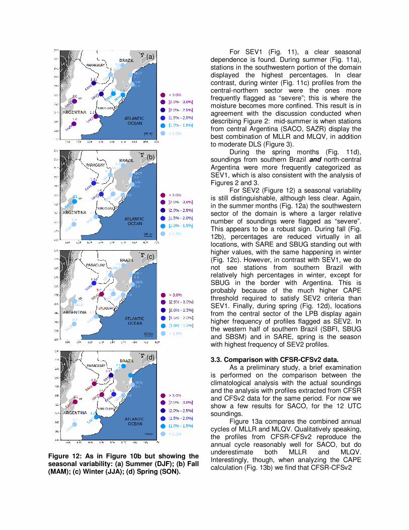
Figure 12: As in Figure 10b but showing the seasonal variability: (a) Summer (DJF); (b) Fall (MAM); (c) Winter (JJA); (d) Spring (SON).

For SEV1 (Fig. 11), a clear seasonal dependence is found. During summer (Fig. 11a), stations in the southwestern portion of the domain displayed the highest percentages. In clear contrast, during winter (Fig. 11c) profiles from the central-northern sector were the ones more frequently flagged as “severe”; this is where the moisture becomes more confined. This result is in agreement with the discussion conducted when describing Figure 2: mid-summer is when stations from central Argentina (SACO, SAZR) display the best combination of MLLR and MLQV, in addition to moderate DLS (Figure 3).

During the spring months (Fig. 11d), soundings from southern Brazil and north-central Argentina were more frequently categorized as SEV1, which is also consistent with the analysis of Figures 2 and 3.

For SEV2 (Figure 12) a seasonal variability is still distinguishable, although less clear. Again, in the summer months (Fig. 12a) the southwestern sector of the domain is where a larger relative number of soundings were flagged as “severe”. This appears to be a robust sign. During fall (Fig. 12b), percentages are reduced virtually in all locations, with SARE and SBUG standing out with higher values, with the same happening in winter (Fig. 12c). However, in contrast with SEV1, we do not see stations from southern Brazil with relatively high percentages in winter, except for SBUG in the border with Argentina. This is probably because of the much higher CAPE threshold required to satisfy SEV2 criteria than SEV1. Finally, during spring (Fig. 12d), locations from the central sector of the LPB display again higher frequency of profiles flagged as SEV2. In the western half of southern Brazil (SBFI, SBUG and SBSM) and in SARE, spring is the season with highest frequency of SEV2 profiles. 3.3. Comparison with CFSR-CFSv2 data.

As a preliminary study, a brief examination is performed on the comparison between the climatological analysis with the actual soundings and the analysis with profiles extracted from CFSR and CFSv2 data for the same period. For now we show a few results for SACO, for the 12 UTC soundings.

Figure 13a compares the combined annual cycles of MLLR and MLQV. Qualitatively speaking, the profiles from CFSR-CFSv2 reproduce the annual cycle reasonably well for SACO, but do underestimate both MLLR and MLQV. Interestingly, though, when analyzing the CAPE calculation (Fig. 13b) we find that CFSR-CFSv2

(a)

(b)

(c)

(d)

Figure 13: Comparing statistics obtained from 12 UTC profiles extracted from CFSR and CFSv2 with the actual 12 UTC soundings for Cordoba (SACO). (a) Same parameter space depicted in Figure 2; (b) box and whiskers plots (10th, 25th, 50th, 75th, and 90th percentiles) comparing CAPE for three distinct air parcels. CFSR-CFSv2 12 UTC profiles were extracted for exactly the same days in which SACO quality-checked 12 UTC profiles were available.

succeeds in reproducing the statistical distribution for the three distinct air parcels. This is a promising result, but still very preliminary. This analysis will be extended for all upper-air stations, for both 00 UTC and 12 UTC soundings, and for several parameters. Once this examination is completed, a better assessment of the suitability of the CFSR-CFSv2 data in providing profiles valid at 18 UTC for the LPB will be possible.

4. SUMMARY AND FINAL REMARKS

In this study a 20-yr climatology of meteorological parameters employed to characterize severe weather environments was generated from operational upper air observations (00 UTC and 12 UTC soundings) conducted in the La Plata Basin (LPB), in subtropical South America. The annual cycles of selected parameters were examined, and relevant percentiles that indicate extreme values of such parameters were determined. The seasonal variation and spatial variability within the LPB of atmospheric profiles that are potentially conducive to severe weather conditions were also addressed in this study.

This short climatology will be useful for South American forecasters in the LPB interested in and responsible for severe weather forecasting. In addition, this study can provide an important data source for regional climate change studies. On the other hand, the lack of afternoon soundings (18 UTC) for the LPB limits, somewhat, our analysis and conclusions.

As this work continues, some aspects to be investigated include:

*Evaluating, with greater detail, atmospheric profiles extracted from CFSR and CFSv2 and from other sources (ERA-Interim), considering as a possible source for 18 UTC profiles;

* Documenting the statistical distribution and spatial/temporal variability of several parameters that SHARPpy computes, including derived parameters such as SCP, STP, etc…

* Investigating the convective activity (or the lack thereof) for profiles flagged as SEV1 and SEV2 in this study.

* Characterizing the frequency of profiles displaying important features such as a northerly/northwesterly low-level jet stream; elevated mixed layer; “loaded-gun” aspect. 5. REFERENCES Atkins, N. T., and R. M. Wakimoto, 1991: Wet microburst activity over the southeastern United States: Implications for forecasting. Wea. Forecasting, 6, 470-482. Blumberg, W. G., K. T. Halbert, T. A. Supinie, P. T. Marsh, R. L. Thompson, and J. A. Hart, 2016: SHARPpy: an open source sounding analysis toolkit for the atmospheric sciences, Bull. Amer. Meteor. Soc., accepted with revisions.

(a)

(b)

Brooks, H. E., J. W. Lee, and J. P. Craven, 2003: The spatial distribution of severe thunderstorm and tornado environments from global reanalysis data. Atmos. Research, 67-68, 73-94. Cecil, D. J., and C. B. Blankenship, 2012: Toward a global climatology of severe hailstorms as estimated by satellite passive microwave imagers. J. Climate, 25, 687–703. Ferreira, V., and E. L. Nascimento, 2016: Convectively-induced severe wind gusts in southern Brazil: surface observations, atmospheric environment, and association with distict convective modes. Preprints, 28th Conf. Severe Local Storms, Amer. Meteor. Soc., Portland/OR (https://ams.confex. com/ams/28SLS/webprogram/ Paper299442.html) Gilmore, M. S., and L. Wicker, 1998: The influence of midtropospheric dryness on supercell morphology and evolution. Mon. Wea. Rev., 126, 943-958. Halbert, K. T., W. G. Blumberg, and P. T. Marsh, 2015: SHARPpy: fueling the python cult. Preprints, 5th Symposium on Advances in Modeling and Analysis Using Python, Phoenix. Matsudo, C. M., and P. V. Salio, 2011: Severe weather reports and proximity to deep convection over Northern Argentina. Atmos. Research, 100, 523-537. Nascimento, E. L., and M. Foss, 2010: A 12-year climatology of severe weather parameters and associated synoptic patterns for subtropical South America. In: Preprints, 25th Conf. Severe Local Storms, Amer. Meteor. Soc., Denver/CO (http://ams.confex.com/ams/pdfpapers/175790. pdf).

, G. Held, and A. M. Gomes, 2014: A multiple-vortex tornado in Southeastern Brazil. Mon. Wea. Rev., 142, 3017-3037. Nesbitt, S. W., P. Borque, K. L. Rasmussen, P. Salio, R. J. Trapp, L. Vidal, M. Rugna, and J. Mulholland, 2016: Severe convection in Central Argentina: storm modes and environments. Preprints, 28th Conf. Severe Local Storms, Amer. Meteor. Soc., Portland/OR (https://ams.confex. com/ams/28SLS/webprogram/Paper301960.html).

Oliveira, M. I., E. L. Figueiredo, V. Ferreira, M. M. Lopes, and E. L. Nascimento, 2016: Evolution and synoptic environment of the 4 July 2014 supercells in Southern Brazil. Amer. Jour. Environ. Eng., 6(4A), 66-73. Rasmussen, E. N., and D. O. Blanchard, 1998: Baseline climatology of sounding-derived supercell and tornado forecast parameters. Wea. Forecasting, 13, 1148-1164. Rasmussen, K., and R. A. Houze, 2011: Orogenic convection in subtropical South America as seen by the TRMM satellite. Mon. Wea. Rev., 139, 2399-2420.

, M. D. Zuluaga, and R. A. Houze, 2014: Severe convection and lightning in subtropical South America. Geophys. Res. Lett., 41, 7359-7366. Romatschke, U., and R. A. Houze, 2010: Extreme Summer convection in South America. J. Climate, 23, 3761-3791. Saha, S., and co-authors, 2010: The NCEP Climate Forecast System Reanalysis. Bull. Amer. Meteor. Soc., 91, 1015-1057. Saha, S., and co-authors, 2014: The NCEP Climate Forecast System version 2. J. Climate, 27, 2185–2208. Vera, C., and co-authors, 2006: The South-American Low-Level Jet Experiment. Bull. Amer. Meteor. Soc., 87, 63-77. Zipser, E. J., D. J. Cecil, C. Liu, S. W. Nesbitt, and D. P. Yorty, 2006: Where are the most intense thunderstorms on earth? Bull. Amer. Meteor. Soc., 87, 1057-1071.