111 measurement of 100 nm and 60 nm particle standards …systems for the minimum particle size...
TRANSCRIPT

1. Introduction
The National Institute of Standards and Technology(NIST) issues Standard Reference Materials (SRM®)for a wide range of particle sizes including 100 nm(SRM® 1963), 0.3 µm (SRM® 1691), 1 µm (SRM®1690), 3 µm (SRM® 1692), 10 µm (SRM® 1960),and 30 µm (SRM® 1961). These standards are monosize
polystyrene spheres suspended in water at a massfraction in the range 0.5 % to 1 %.
The focus of this paper is the measurement results anduncertainty analyses for two batches of particles withnominal sizes of 100 nm and 60 nm. The 60 nm size isneeded in the calibration of scanning surface inspectionsystems for the minimum particle size detected. Thesedevices are used in the semiconductor industry to
Volume 111, Number 4, July-August 2006Journal of Research of the National Institute of Standards and Technology
257
[J. Res. Natl. Inst. Stand. Technol. 111, 000-000 (2006)]
Measurement of 100 nm and 60 nm ParticleStandards by Differential Mobility Analysis
Volume 111 Number 4 July-August 2006
George W. Mulholland,Michelle K. Donnelly, Charles R.Hagwood, Scott R. Kukuck, andVincent A. Hackley
National Institute of Standardsand Technology,Gaithersburg, MD 20899
and
David Y. H. Pui
Department of MechanicalEngineering,Particle Technology Laboratory,University of Minnesota,Minneapolis, MN 55455
[email protected]@[email protected]@nist.gov
The peak particle size and expandeduncertainties (95 % confidence interval)for two new particle calibration standardsare measured as 101.8 nm ± 1.1 nm and60.39 nm ± 0.63 nm. The particle samplesare polystyrene spheres suspended infiltered, deionized water at a mass fractionof about 0.5 %. The size distributionmeasurements of aerosolized particlesare made using a differential mobilityanalyzer (DMA) system calibrated usingSRM® 1963 (100.7 nm polystyrenespheres). An electrospray aerosol generatorwas used for generating the 60 nm aerosolto almost eliminate the generation ofmultiply charged dimers and trimers andto minimize the effect of non-volatile con-taminants increasing the particle size. Thetesting for the homogeneity of the samplesand for the presence of multimers usingdynamic light scattering is described. Theuse of the transfer function integral in thecalibration of the DMA is shown to reducethe uncertainty in the measurement ofthe peak particle size compared to theapproach based on the peak in theconcentration vs. voltage distribution. Amodified aerosol/sheath inlet, recirculatingsheath flow, a high ratio of sheath flow tothe aerosol flow, and accurate pressure,temperature, and voltage measurementshave increased the resolution and accuracyof the measurements. A significantconsideration in the uncertainty analysis
was the correlation between the slipcorrection of the calibration particle andthe measured particle. Including thecorrelation reduced the expandeduncertainty from approximately 1.8 % ofthe particle size to about 1.0 %. Theeffect of non-volatile contaminants in thepolystyrene suspensions on the peakparticle size and the uncertainty in the sizeis determined. The full size distributionsfor both the 60 nm and 100 nm spheresare tabulated and selected mean sizesincluding the number mean diameterand the dynamic light scattering meandiameter are computed. The use of theseparticles for calibrating DMAs and formaking deposition standards to be usedwith surface scanning inspection systemsis discussed.
Key words: differential mobility analysis;dynamic light scattering; electricalmobility; electrospray aerosol generation;particle size calibration standards; transferfunction.
Accepted: June 20, 2006
Available online: http://www.nist.gov/jres

measure the number of contaminant particles of size60 nm and larger on a bare silicon wafer. The 100 nmparticle discussed here is intended to replace SRM®1963, for which individual spheres in many of thepreviously prepared vials have formed agglomerates.In many cases a large floc was visible to the eye in the5 mL vials. Quantitative evidence for the presence ofdimers and trimers was obtained by Fitzpatrick [1]using a disk centrifuge. Five samples were analyzed,and, in four of the five, the fraction of multimersexceeded 30 %. The presence of multimers was alsoevident from dynamic light scattering (DLS) mea-surements. While the individual peaks were notresolved, the peak size as interpreted by DLS wastypically 30 % to 70 % greater than the nominalmonomer particle size.
When evidence of agglomeration was first quantifiedin SRM® 1963, a decision was made to modify theCertification of Analysis to state that “the standardis not appropriate for applications where monosize,unagglomerated spheres are necessary.” The sampleswere still useful for calibration of electron microscopesand for generating a monosize aerosol using a differen-tial mobility classifier (DMA), since there was still ahigh enough concentration of monomers present.However, there was evidence from the semiconductorindustry that the use of SRM® 1963 particles as a dep-osition standard in an agglomerated state was problem-atic. Because of the importance of the 100 nm sizerange in the semiconductor industry for the calibrationof surface scanning inspection systems and because ofthe need for unagglomerated spheres in calibratingoptical scattering instruments such as dynamic lightscattering instruments, a decision was made to issue areplacement for SRM® 1963.
The general approach to the measurement of particlesize and measurement uncertainty is similar to that usedby Mulholland et al. [2]. In the current study, SRM®1963 was used for calibrating the differential mobilityanalyzer (DMA), while in the earlier study [2] a mono-size aerosol with a number mean size of 895 nm(SRM® 1690) was used to calibrate the classifier.Among the remaining SRM® 1963 samples, severalunagglomerated samples were found and used for thecalibration.
The calibration approach and measurement methodhave been modified since the earlier study [2] toaccount for the effect of the finite width of the DMAtransfer function on the measured peak particle size.This approach, which is similar to that of Ehara et al. [3],is used to assess the error resulting from the use of the
simpler approach in [2]. The theoretical approach andthe numerical methods used are presented in Sec. 2.
The physical properties used to measure the particlesize including slip correction, electron charge, chargingprobability as a function of particle diameter, viscosity,and mean free path are presented in Sec. 3 along withthe formulas used to compute the quantities for a rangeof conditions. The estimated uncertainties in the prop-erties are included.
There have been several improvements in the instru-mentation since the earlier study. The use of a modifiedaerosol/sheath inlet, a recirculating sheath flow, and a40 to 1 ratio of sheath flow to the aerosol flowincreased the resolution and accuracy of the measure-ments. The uncertainty in the pressure and temperaturemeasurement have been reduced by at least a factor often and the uncertainty in the DMA voltage has beenreduced by almost a factor of two for the 100 nm spheremeasurements. In addition, a pneumatic nebulizer witha more constant output was used for the 100 nmspheres and an electrospray generator was used for the60 nm spheres to reduce the effects of multiply chargedmultimers and nonvolatile impurities in the particle-water suspension. These new features together with thegeneral measurement approach are presented in Sec. 4.The characteristics of the 100 nm spheres and 60 nmspheres are presented in Sec. 5 along with a descriptionof the sample preparation for use with the DMAmeasurement system.
A number of samples were selected at random withrepeat measurements made on each sample to assessthe homogeneity of the samples in terms of the peakparticle size. A series of measurements were then madeon a single sample to determine the peak particle sizebased on at least three repeat measurements over eachof three different days. For every sample measurementthere was also a calibration measurement. The meas-urement approach and analysis are described in Sec. 6and the experimental design, statistical test for samplehomogeneity, and the analysis of the Type A uncertain-ty [4], which is computed by statistical methods, arepresented in Sec. 7.
The Type B uncertainty analysis, which is usuallybased on scientific judgment, is presented in Sec. 8.One significant improvement in the uncertainty analy-sis is accounting for the correlation between the slipcorrection for the measured particle, either the 60 nm or100 nm, and the slip correction of the SRM® 1963particles used in calibrating the DMA. Other importantconsiderations in the uncertainty analysis are the driftin the number concentration during the measurement of
258
Volume 111, Number 4, July-August 2006Journal of Research of the National Institute of Standards and Technology
the number concentration versus voltage, the overlapbetween singlet monomers and doublet trimers, and thepresence of non-volatile contaminants in the polystyrenesphere suspension. The 100 nm and 60 nm sphere dia-meters as aerosols are corrected for the residuer layer onthe SRM® 1963 spheres.
The results of dynamic light scattering to assess thepresence of multiplets in the sample vials are presentedin Sec. 9. Dynamic light scattering will be used in thefuture to verify that agglomeration has not taken placewithin the sample. Transmision electron microscopyresults for the 60 and 100 nm spheres are presented inSec. 10.
The particle size measured in this study is the modaldiameter, i.e. the peak in the number size distribution.The choice of the modal diameter for certification ismotivated by the wide use of DMA’s in the depositionof monodisperse particles on wafers, operated at thevoltage corresponding to the peak transmission(throughput). Results are also provided in Sec. 11 forthe number mean diameter and the so called Z-aver-aged diameter measured by dynamic light scattering.The full size distribution for both the 60 nm and 100nm spheres is tabulated. Also in Sec. 11, the estimatedsize distribution of particles deposited on a waferresulting from operating a DMA at the peak voltage forthe 60 nm spheres or 100 nm spheres is presented.
2. Theoretical Background
The approach used in this study is to determine thesize distribution of particles by measuring their electri-cal mobility, Zp. The relationship between particlediameter, Dp, and electrical mobility can be obtained byperforming a balance between the electric force,assumed to be in the x direction, and the drag force ona singly charged particle initially at rest.
(1)
where η is the gas viscosity, e is the electron charge, andC(Dp) is the Cunningham slip correction factor that cor-rects for non-continuum gas behavior on the drag forcefor small particles. The particle will initially accelerate inresponse to the electric field Ex and approach the veloci-ty vx for which the drag force balances the electric force.Solving for the ratio of the velocity to the electric field,the definition of Zp, one obtains an expression for Zp as afunction of particle diameter:
(2)
This equation provides the basis for measuring theparticle size distribution via electrical mobility meas-urements. The size dependence of the electrical mobil-ity ranges from an inverse dependence on diameter forsizes large compared to the mean free path of the gas(Stokes limit) to an inverse quadratic dependence forparticle sizes much smaller than the mean free path(free molecular limit).
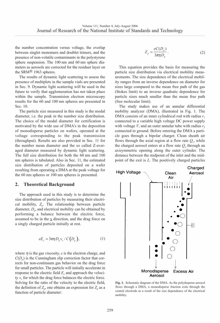
The study makes use of an annular differentialmobility analyzer (DMA), illustrated in Fig. 1. TheDMA consists of an inner cylindrical rod with radius r1
connected to a variable high voltage DC power supplywith voltage V, and an outer annular tube with radius r2
connected to ground. Before entering the DMA a parti-cle goes through a bipolar charger. Clean sheath airflows through the axial region at a flow rate Qc, whilethe charged aerosol enters at a flow rate Qa through anaxisymmetric opening along the outer cylinder. Thedistance between the midpoint of the inlet and the mid-point of the exit is L. The positively charged particles
Volume 111, Number 4, July-August 2006Journal of Research of the National Institute of Standards and Technology
259
( )3 / ,x p x peE D v C Dπη=
( ).
3p
pp
eC DZ
Dπη=
Fig. 1. Schematic diagram of the DMA. As the polydisperse aerosolflows through a DMA, a monodisperse fraction exits through thecentral electrode as a result of the size dependence of the electricalmobility.

move radially towards the center rod under the influ-ence of the electric field. Near the bottom of the classi-fying region, a flow consisting of nearly-monodisperseaerosol exits through a slit in the center rod at a flowrate Qa.
2.1 Convolution Integral and DMATransfer Function
Knutson and Whitby [5] derived an expression forthe number of particles, N(V), exiting the DMA at volt-age V involving an integral over the product of theDMA transfer function Ω and the mobility size distri-bution function F(Zp), where F(Zp)dZp is equal to thenumber of particles with mobility between Zp andZp + dZp. The result for the case where the inlet aerosolflow is equal to the outlet flow is given by:
(3)
It is assumed that N(V) is the part of the DMAspectrum for singly charged particles, and it is alsoassumed that the size distribution is relatively narrowwith a standard deviation less than 15 % of the peakdiameter, so that only singly charged particles are pres-ent at the peak. The transfer function Ω for the DMAoperating at voltage V is defined as the probability thata charged particle entering the DMA with electricmobility Zp will leave through the sampling slit. Thetransfer function Ω has a triangular shape with a peakvalue of 1 and, for a perfectly monodisperse aerosol, allthe aerosol entering the DMA exits through the slit inthe center electrode for the voltage corresponding to thepeak in the transfer function.
Our primary interest is in obtaining the diameter sizedistribution, G(Dp), where G(Dp)dDp is equal to thenumber of particles per cm3 with diameter between Dp
and Dp + dDp. In one case, we will use a known dia-meter distribution to calibrate the DMA and, in anothercase, we will be using the DMA to measure the peak inthe diameter distribution for two new particle sizecalibration standards. The relationship between F(Zp)and G(Dp) is given by:
(4)
The quantity p(Dp) is the probability that a particlewith diameter Dp carries one elementary unit of charge.The absolute value of the derivative in Eq. (4) reflectsthe fact that F(Zp) and G(Dp) are positive definite quan-tities but the inverse dependence of the mobility on thediameter results in a negative derivative.
Substituting the expression for F(Zp) into Eq.(3), weobtain:
(5)It is convenient when carrying out the numerical
integration of Eq. (5) for a given size distribution func-tion to express the integral in terms of the dimension-less mobility x defined as:
(6)
Here, Λ is a geometric factor based on the inner andouter radius and the length of the classifying region ofthe DMA,
(7)
The transfer function Ω can be convenientlyexpressed in terms of both x and the ratio of the aerosolflow to the sheath flow, δ = Qa / Qc,
(8)
The transfer function is triangular and increasesfrom zero to 1 and then decreases back to zero overa range of x equal to 2δ. The standard deviationof the transfer function divided by the average value of
is equal to This provides a conven-ient dimensionless measure of the DMA resolution interms of mobility. One can see from the definition of δthat the measurement resolution increases as the valueof the ratio of the aerosol flow to sheath flow isdecreased. In the measurements described below, thevalue of δ was 0.025, corresponding to a sheath flow of20 L/min and an aerosol flow of 0.5 L/min. For thisvalue of δ, = 0.0102.
The standard deviation of the transfer functionexpressed in terms of diameter is a more convenientvalue for comparison with the standard deviation of thesize distribution. From Eqs. (2) and (6), one can derivethe following relationship:
(9)
Volume 111, Number 4, July-August 2006Journal of Research of the National Institute of Standards and Technology
260
0
( ) ( ) ( ) .p p pN V Z V F Z dZ∞
= Ω ⋅∫
( ) ( )( ) ( )( ) / .p p p p p p pF Z G D Z p D Z dD dZ=
0
( ) ( ) ( ( )) ( ( )) / .p p p p p p p pN V Z V G D Z p D Z dD dZ dZ∞
= Ω ⋅∫
2.p
c
Z Vx
QπΛ
=
2 1/ ln( / ) .L r rΛ =
( ) 0 1x x δΩ = < −(1 )( ) 1 1 1xx xδ
δ−Ω = − − ≤ <
(1 )( ) 1 1 1xx x δδ−Ω = + ≤ ≤ +
( ) 0 1 .x x δΩ = > +
( ), ,Trx xσ / 6 .δ
( )Tr xσ
( )( )
1
1 .p pp
p p
C' D DdD dxD x C D
− = −
Replacing the reduced differentials with the correspon-ding standard relative deviations, one obtains
(10)
Assuming nominal temperature and pressure of themeasurement condition to be 23 °C and 101.33 kPa,respectively, the computed value of is 0.0058for the 101.6 nm spheres and 0.0055 for the 60.5 nmspheres.
With the transfer function expressed in terms of x, itis also convenient to express the integral in Eq. (5) asan integral over x. From Eq. (9), one can also derive thefollowing relationship:
(11)
Using Eq. (8) and Eq. (11), the integral can then beexpressed in terms of x with the result:
(12)
A computer program was written to carry out the inte-gration. The integrations were carried out both for cali-brating the DMA and for estimating the accuracy of anapproximate method given below for determining thepeak particle size for an unknown size distribution. Theexpression used for the slip correction is given in Sec. 3.
2.2 Calibration of DMA and Determination ofPeak Particle Size
The DMA is calibrated using the accurately sizedSRM® 1963 with G(Dp) assumed Gaussian and havinga mean size of 100.7 nm and an estimated standarddeviation equal to 2.0 nm. The number concentration ismeasured versus voltage and the peak voltage is deter-mined. This value is compared with the prediction ofEq. (12) where the integration limits are set by the flowratio of δ = 0.025. If the sheath flow, Qc, used in theprediction differs from the actual flow, then the meas-ured peak voltage will not agree with the predicted
peak voltage. It is seen from Eq. (6), however, that theflow rate Qc can be adjusted by the ratio of the meas-ured voltage to the predicted voltage so that the mobil-ity Zp is the same for both the measurement and thepredicted value. This adjustment, therefore, calibratesthe parameters used in the calculations to actual opera-tional conditions.
It is also possible that the geometric factor is in error.In this case, the above correction would be a combinedcorrection factor for both the flow and the geometricfactor. The basis for using this approach rather thanusing the directly measured flow and geometric para-meter is that the combined uncertainty is lower using anaccurately known calibration standard versus using themeasured values together with uncertainty in the flowand in the geometric factor.
2.2.1 Approximation 1
In general, the determination of the size distributionrequires the inversion of Eq. (12). For the case in whichthe size distribution is broad and changing slowly withdiameter, an approximate expression can be obtainedfor G(Dp). In this case, the transfer function variesmuch more rapidly with x than do the other functionsappearing in the integrand of Eq. (12). The other func-tions are, therefore, evaluated at the value of Dp corre-sponding to the peak in the transfer function, x = 1, forthe given voltage. This leads to the following result:
(13)
The integral of the transfer function is δ, simply thearea of a triangle with height 1 and base 2δ (see Eq. (8)).Thus, from Eq. (13), the following explicit expressionoriginally proposed by Knutson [6] approximates the sizedistribution:
(14)
The mobility for x = 1 corresponding to voltage V iscomputed from the following equation:
(15)
Volume 111, Number 4, July-August 2006Journal of Research of the National Institute of Standards and Technology
261
( ) ( ) ( )( )
1
1 .p pT Tr p r
p
C' D DD x
C Dσ σ
− = −
( )( )
1
1 1/ .pp p p
pp
C DdD dZ dZ dx
x DC D
−′
= −
( )( ) ( )( )1
1
(1 )( ) 1 p pxN V G D x p D x
δ δ−
− = − ∫
( )( )
11
1
1 1 (1 )1p
pp
C D xdxx DC D
δ
δ
−+′ − − + + ∫
( ) ( )( ) ( )( )
1
1 1( ) .pp p
pp
C DG D x p D x dx
x DC D
−′
− ( )( ) ( )( ) ( )( )
1
1
1( ) 1 1 pp p
pp x
C DN V p D x G D x
DC D
−
=
′ = = = −
1 1
1 1
(1 ) (1 )1 1 .x xdx dxδ
δ δ δ
+
−
− − × − + − ∫ ∫
( )( ) ( ) ( )( ) ( )( )11 / 1 . p
p ppp
C DG D x N V p D x
DC Dδ
′ = = − =
( ) ( ) ( )2 1ln /1 / 2 .
2c
p c
Q r rZ x Q V
VLπ
π= = = Λ
( )Tr pDσ
The value of Dp corresponding to Zp is computed basedon Eq. (2). A description of the iterative methodused to solve this implicit equation for Dp is given inAppendix A.
To assess the accuracy of using Eq. (14) in computingG(Dp), a comparison will be made for the peak in the sizedistribution obtained using this approximate methodversus the true peak in the size distribution.
2.2.2 Approximation 2
A widely used calibration and measurement method[7] is to measure the peak voltage for the 100.7 nm SRMspheres and the unknown particles. From Eq. (15), themobility of the unknown particle, can be expressedas the mobility of the 100.7 nm particle, multi-plied by the ratio of the peak voltages,
(16)
with the value of computed from Eq. (2). Threeassumptions are used in this approach. First, the peak inthe mobility distribution for the SRM is assumed to bethe mobility corresponding to the peak in the diameterdistribution of the SRM. Secondly, the peak in themeasured size distribution is assumed to be the diame-ter inferred from the peak in the voltage distribution.The third assumption is that the size distribution issymmetric about x = 1.
2.2.3 Accuracy of Approximate Methods
Now let us compare the accuracy of the above approx-imate approaches for size distributions close to that ofthe 60 nm and 100 nm spheres. We assume size distribu-tions that are Gaussian with peak diameters of 60.7 nmand 101.6 nm and with standard deviations of 4.3 nmand 2.6 nm. The number concentration is computed as afunction of voltage using Eq. (12). We use this as “data”and compute the peak size using the two approximationsdescribed above. As seen in Table 1 for the 60.7 nmspheres, Approximation 1 is significantly more accurate
with a difference of less than 0.01 % compared to a0.71 % difference for Approximation 2. The smaller the ratio of the reduced standard deviation of the transferfunction to that of the size distribution function, thebetter Approximation 1 should be. This is the case for theexample in Table 1. For the 60 nm sphere the ratio, 0.08,is about three times smaller than that for the 100 nmsphere and the relative difference from the correct dia-meter is about five times smaller for the 60 nm spheres.However, in both cases the agreement with the correctvalue is within 0.05 %. Ehara et al. [3] have investigatedthe accuracy of Approximation 1 and 2 for the case ofskewed Gaussian distributions with a peak particle sizeof 100 nm. For Approximation 1, the number mean dia-meter was accurately retrieved even for size distributionswith widths small relative to the transfer function width.For Approximation 2, a significant deviation was ob-served for broad size distributions with the standarddeviation /mean size > 0.05. This result is consistent withour analysis that both Approximations work wellfor the narrowly distributed 100 nm spheres, but thatApproximation 2 does not work as well for the morebroadly distributed 60 nm spheres.
3. Physical Properties: ExpressionsUsed and Estimated Uncertainty
The relevant physical parameters are evident fromlooking at three key equations for making size measure-ments using the DMA. The first relates the electricalmobility to particle diameter, Eq. (2), and includes theelectron charge, viscosity, and the slip correction, whichin turn depends on the mean free path. The mobility atthe peak in the transfer function [Eq. (6)) evaluated atx = 1] is a function of the classifier geometry includingthe inner and outer diameter and the length of the classi-fier region and of the sheath flow. The predicted particleconcentration as a function of voltage depends on thebipolar charging function, p(Dp) as seen from Eq. (12)and on the number concentration measurement.
Volume 111, Number 4, July-August 2006Journal of Research of the National Institute of Standards and Technology
262
,upZ
,SRMpZ
( ) ( )1 1 / ,u SRM SRM up p p pZ x Z x V V= = =
,SRMpZ
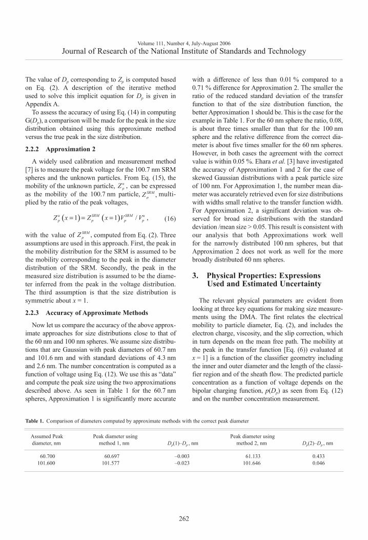
Table 1. Comparison of diameters computed by approximate methods with the correct peak diameter
Assumed Peak Peak diameter using Peak diameter usingdiameter, nm method 1, nm Dp(1)–Dp , nm method 2, nm Dp(2)–Dp , nm
60.700 60.697 –0.003 61.133 0.433101.600 101.577 –0.023 101.646 0.046

3.1 Charge of an Electron – e
The magnitude of the charge on the electron and itscombined uncertainty (1 standard deviation) is equal to(1.6021892 ± 0.0000046) × 10–19 C [8]. The standardrelative uncertainty is about 3 × 10⁻⁴ % and is negligiblein assessing the overall uncertainty in the particlediameter.
3.2 Viscosity – ηη
In 1945, Birge [9] reported the weighted average valueof the viscosity of dry air at 23.00 °C as η0 = (1.83245 ±0.00069) × 10–5 kg m–1 s–1 from six different results,correcting for temperature by using the Sutherland equa-tion. This air viscosity value was used in the certificationmeasurements of SRM® 1963 [2]. For consistency, wealso consider the Birge result as the reference viscosityfor this study. Once the reference viscosity at 23.00 °C isdetermined, the viscosity for other temperatures can beobtained using the Sutherland formula as discussed byAllen and Raabe [10],
(17)
where T0 is the absolute reference temperature(296.15 K) and T is the absolute temperature.
The value of the viscosity of dry air at 23.00 °C fromBirge [6], has a 0.038 % relative standard uncertainty.The air flowing through the DMA has an estimated 7 %relative humidity. The decrease in the viscosity fromthe addition of water is estimated as 0.080 % based onthe viscosity of water and its volume fraction of the air.This value of 0.080 % is taken as the standard relativeuncertainty in the air viscosity resulting from thepresence of water vapor. Computing the standard rela-tive combined uncertainty of viscosity as the root-sum-of-squares, a value of 0.089 % is obtained. As isseen in Sec. 7, the uncertainty in the viscosity does notaffect the particle diameter uncertainty when calibrat-ing the DMA with a particle of known size.
3.3 Slip Correction – C(Dp) and Mean Free Path – λλ
The Cunningham slip correction factor, which cor-rects for noncontinuum gas behavior on the motion ofsmall particles, is given by
(18)
where the Knudsen number is twice the mean free pathof air divided by the particle diameter (Kn = 2λ /Dp), A1,A2, and A3 are dimensionless constants, and A is termed
the slip correction parameter. The quantity A is of keyimportance in the uncertainty analysis in Sec. 8.2. Inour analysis two sets of values are used for the slipcorrection constants: A1 = 1.142, A2 = 0.558, and A3 =0.999 (Allen et al., 1985 [11]) and A1 = 1.165, A2 =0.483, and A3 = 0.997 (Kim et al., [12]). The firstexpression, which was used in the measurement ofSRM® 1963, was obtained using a Millikan apparatuswith monosize polystyrene spheres having diameters ofabout 1 µm, 2 µm, and 4 µm. The second expressionwas obtained using reduced pressure measurementswith a Nano-DMA1 on accurately sized calibrationparticles with diameter of 269 nm, 100.7 nm, and19.90 nm [12]. Over the Knudsen number range from1.35 to 2.25, which corresponds to a diameter rangefrom 60 nm to 100 nm, the combined relative standarduncertainty in the Kim et al. [12] expression is 1.0 % orslightly less. The study by Allen et al. [11] does notcontain an estimate of the combined relative standarduncertainty. Both of these sets of values will be used incomputing the peak diameter.
The mean free path λ is needed to compute the slipcorrection. It cannot be directly measured, but insteadis determined from the kinetic theory relationship forviscosity,
(19)
where φ is a constant dependent upon the intermolecu-lar potential, ρ is the gas density, and c– is the meanvelocity of gas molecules. The value of φ = 0.491 isderived by assuming hard elastic spheres with repulsiveforces between the molecules [13]. The certificationmeasurements of SRM® 1963 [2] used λ0 = 67.3 nmfor the mean free path of air at 101.325 kPa and23.00 °C. Once the reference value of λ0 has beenchosen, it can be corrected for any pressure andtemperature using Willeke’s relation [14]
(20)
where
Volume 111, Number 4, July-August 2006Journal of Research of the National Institute of Standards and Technology
263
1.5
00
0
110.4 K,
110.4 KTT
T Tη η
+= +
( ) [ ]1 2 31 exp( / 1 ,p n n nC D K A A A K K A= + + − = + 1 Certain commercial equipment, instruments, or materials are iden-tified in this paper to specify adequately the experimental procedure.Such identification does not imply recommendation or endorsementby the National Institute of Standards and Technology, nor does itimply that the materials or equipment identified are necessarily thebest available for the purpose.
,cη φρ λ=
( )( )
000
0
1 110.4 K /,
1 110.4 K /TPT
T P Tλ λ
+ = +

λ0 = 67.3 nm, for air at T0, P0
T0 = reference temperature, 296.15 KP0 = reference pressure, 101.33 kPaT = air temperature inside the classifierP = air pressure inside the classifier.
Equation (20) is used in the subsequent analysis for themean free path of air.
3.4 Geometric Factors
The critical dimensions for the DMA are the innerradius r1 = 0.937 cm, the outer radius r2 = 1.958 cm,and the classifying length L = 44.44 cm. These dimen-sions were measured at NIST for the DMA used in thisstudy. The quantity Λ defined in Eq. (7) has a value of0.60299 cm. The uncertainty in this value is not need-ed, since the DMA is calibrated with a particle ofknown size. An error in either the geometric dimensionor in the volumetric flow rate is corrected by this cali-bration as discussed in Sec. 2.2.
3.5 Flow Rate
The nominal sheath and aerosol flow rates are20 L/min and 0.5 L/min. The actual sheath flow rate iscalibrated before each size-distribution measurement.The average change in the flow between two successivecalibrations is 0.1 %. The leakage rate in the recircula-tion system is measured to be 0.020 cm3/s. This cor-responds to about 0.25 % of the 0.5 L/min aerosol flow[15].
3.6 Flow Ratio
The ratio of the aerosol flow to the sheath flow is0.025 based on the nominal flows. The uncertainty inthe flow ratio is + 2 %, – 7 %. The asymmetry arisesfrom the corrected sheath flow being about 2 % largerthan the nominal value of 20 L/min.
3.7 Charging Probability
The quantity p(Dp), the probability that a particle ofsize Dp has a single unit of positive charge, is neededboth in computing the size distribution function inEq. (14) and also in Eq. (11) for calibrating the DMAwith a particle of known size. The following expressionfor p(Dp), determined by Wiedensohler [16], is used inour analysis:
(21)
where Dunit = 1 nm, a0 = –2.3484, a1 = 0.6044, a2 =0.4800, a3 = 0.0013, a4 = –0.1553 and a5 = 0.0320. This
approximate expression is within 3 % of the valuepredicted by Fuch’s theory [17] for particle sizes of50 nm, 70 nm, and 100 nm: The reduced difference,[p(approximate)—p(Fuchs)]/p(Fuchs), equals –2.6 %for 50 nm, 0.7 % for 70 nm, 1.6 % for 100 nm.
4. Particle Sizing Facility
The equipment comprising the DMA measurementsystem consists of five components: the aerosol gener-ator, the electrostatic classifier, the condensation parti-cle counter, the recirculation system, and the dataacquisition system. All of the components, except therecirculation system and a modified aerosol/sheathinlet, are commercially available equipment. Theequipment and methodology used here are similar tothat used previously in performing particle calibrationmeasurements [18].
4.1 Aerosol Generation
Two types of aerosol generators were used. A pneu-matic nebulizer was used for generating the new 100nm spheres and an electrospray generator was used forthe 60 nm spheres.
4.1.1 Pneumatic Generator
The 100 nm polystyrene sphere aerosol is generatedusing an Aeromaster Constant Number PSL StandardParticle Generator manufactured by JSR Corporation.The generator is a pneumatic atomizer that operates byusing filtered compressed (100 kPa gauge) air to gener-ate a high velocity gas jet, which, in turn, creates a lowpressure region near the tube exit. The pressure imbal-ance acts to draw liquid with suspended PSL spheresinto this region. The high air velocity breaks up theliquid into a wide range of droplet sizes with largedroplets impinging on the wall and dripping into a con-tainer, and smaller droplets flowing with the air stream.Fresh liquid is constantly drawn into the spray regionresulting in a steadier particle concentration than wouldoccur with dripping of the impinging drops back intothe liquid reservoir. Another feature that improvesthe generator’s stability is a temperature-controlledcapillary feed line.
The aerosol passes through a heated tube where theliquid evaporates leaving only the solid PSL particlesas an aerosol. The flow then enters a diluter where itjoins a clean air stream. The flow passes through abipolar charger to reduce the droplet charge. Theaerosol flow of about 14 L/min then enters an integrat-ing chamber. The chamber has a volume of approxi-mately 14 L and serves to dampen any short term fluc-
Volume 111, Number 4, July-August 2006Journal of Research of the National Institute of Standards and Technology
264
5
10 100
log ( ) log ,i
pp i
i unit
Dp D aD=
=
∑
tuation in the aerosol concentration. This generatormaintains a steady particle concentration typicallywithin 2 % during a fifteen minute voltage scan.
The charged flow leaves the chamber and reaches theclassifier via a path containing regulating vents. Thevents are adjusted to set the desired flow rate enteringthe classifier, while the remaining flow is sent to theexhaust. This is necessary since the aerosol generatorsupplies a flow of approximately 16 L/min (267 cm3/s)while the typical flow into the classifier is less than2 L/min (33 cm3/s).
4.1.2 Electrospray Generator
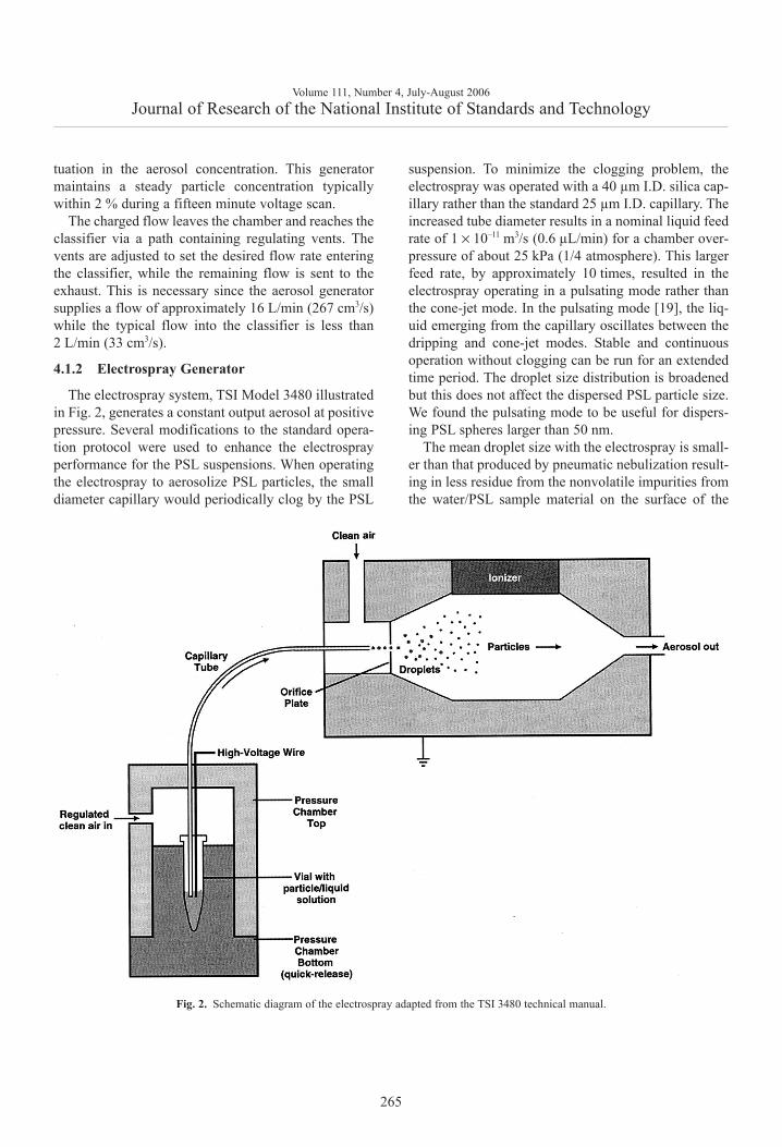
The electrospray system, TSI Model 3480 illustratedin Fig. 2, generates a constant output aerosol at positivepressure. Several modifications to the standard opera-tion protocol were used to enhance the electrosprayperformance for the PSL suspensions. When operatingthe electrospray to aerosolize PSL particles, the smalldiameter capillary would periodically clog by the PSL
suspension. To minimize the clogging problem, theelectrospray was operated with a 40 µm I.D. silica cap-illary rather than the standard 25 µm I.D. capillary. Theincreased tube diameter results in a nominal liquid feedrate of 1 × 10–11 m3/s (0.6 µL/min) for a chamber over-pressure of about 25 kPa (1/4 atmosphere). This largerfeed rate, by approximately 10 times, resulted in theelectrospray operating in a pulsating mode rather thanthe cone-jet mode. In the pulsating mode [19], the liq-uid emerging from the capillary oscillates between thedripping and cone-jet modes. Stable and continuousoperation without clogging can be run for an extendedtime period. The droplet size distribution is broadenedbut this does not affect the dispersed PSL particle size.We found the pulsating mode to be useful for dispers-ing PSL spheres larger than 50 nm.
The mean droplet size with the electrospray is small-er than that produced by pneumatic nebulization result-ing in less residue from the nonvolatile impurities fromthe water/PSL sample material on the surface of the
Volume 111, Number 4, July-August 2006Journal of Research of the National Institute of Standards and Technology
265
Fig. 2. Schematic diagram of the electrospray adapted from the TSI 3480 technical manual.

PSL sphere after the water has evaporated. A study byMulholland et al. [20] found that the PSL sphere dia-meter obtained using electrospray was about 1 %smaller than that obtained by pneumatic nebulizationfor 100 nm spheres and about 5 % smaller for 50 nmspheres. This study was carried out with a prototypeelectrospray with a smaller capillary diameter, 25 µm,and for a different pneumatic nebulizer, which isthought to produce a larger mean droplet size than thatproduced by Aeromaster. Another set of measurementswas made using the Aeromaster and the current electro-spray with a 25 µm capillary [7]. The PSL diametergenerated with the electrospray was 2.5 % smaller for55 nm spheres and 3.9 % smaller with 64 nm sphere.The uncertainty in these differences is about ± 1.3 %;that is, 3.9 % ± 1.3 % and 2.5 % ± 1.3 %. During a setof screening measurements made the month after the100 nm certification measurements, the peak particlesize was measured for nominal 64 nm spheres usingboth the Aeromaster and the current configuration ofthe electrospray with the 40 µm diameter capillary. Itwas found that the PSL sphere size obtained with theelectrospray was about 3 % to 4 % smaller than thevalue obtained with the pneumatic nebulizer. Whilethere were only two repeats using each generator, theresult is consistent with the previous studies [20, 7] andis a strong indication that there is less of a residue effectwith electrospray compared to the pneumatic atomizer.Additional measurements of the residue layer are pre-sented in Sec. 8.3.8.
A flow of 33.3 cm3/s (2 L/min) of dry-filtered airenters the spray system. A co-flow of CO2, which iscommonly used to prevent corona discharge, was notused in our experiments because of the difficulty inaccurately determining the viscosity of such a gasmixture. As the particles flow through the orifice (SeeFig. 2) they are exposed to a bi-polar distribution ofions produced by 370 MBq Po210, which produces αradiation. The particles acquire a Boltzmann chargedistribution described by Eq. (21).
The sample is introduced into the cell, pressureapplied, and the air flow set. The voltage is increased,and the droplets are observed through the viewing win-dow illuminated by a light emitting diode. The voltageis increased until the current output displayed by thegenerator varies by less than 2 nA over the nominal10 min required for measuring the size distribution.Typically the voltage was about 1.5 kV, the current wasabout 120 nA, and the spray pattern appeared as a pul-sating tip. The voltage range used in these tests is lowerthan typically used with the electrospray. This is in parta result of not using the CO2 gas, which resulted in an
onset of corona breakdown at a lower voltage. In somecases the voltage was increased to 1.8 kV or 2.2 kV toobtain stable behavior. The resulting peak number con-centrations were in the range of (200 – 450) particlesper cm3. The particle number concentration for a fixedDMA voltage was observed to drift by as much as 10 %over a measurement period. Measurements were madeat a voltage close to the peak voltage at the start of theexperiment, at the middle, and at the end to estimate alinear drift in the concentration over the course of theexperiment. All the number concentration data wereadjusted with the linear fit to give the estimated con-centration at the time of the peak measurement. Theseadjustments were made for both the SRM calibrationmeasurements used to find the corrected flow and forthe 60 nm sphere measurements.
Once started, the system generally provides a steadyoutput of particles. Over a five day period during whichthe electrospray was run on the order of four hours aday, one capillary had to be replaced because of clog-ging. The filtering of the suspension of particles inthe electrolyte with a 1.2 µm pore size filter may havehelped minimized the particle clogging. The otherstandard precaution of running particle free electrolytefor one hour in the dripping mode after the test to cleanparticles away from the tip was used. Also, a 1 L accu-mulator was used directly after the generator to reduceconcentration fluctuations.
4.2 DMA
The DMA used in these experiments is a model3071A Electrostatic Classifier manufactured by TSIIncorporated. The DMA separates aerosol particlesbased on their electrical mobility as described in Sec. 2.This allows for a flow of monosize particles to exit theclassifier. The DMA measurement system contains abipolar charger (TSI Model 3077 Aerosol Neutralizer)consisting of 7.4 × 10⁷ Bq (2 mCi) of Kr 85 radioactivegas contained in a capillary tube. Here the particles col-lide with bipolar ions resulting in an equilibrium chargedistribution that is a function of the particle size. Theprobability of a sphere having a single charge is givenabove by Eq. (21). For example, 100 nm particleswould emerge from the bipolar charger with 42 % ofthe particles uncharged, 21 % with a +1 charge, 27 %with a –1 charge, and smaller percentages with multi-ply charged particles. The charger is removed whenusing the electrospray, since it already contains a bi-polar charger.
After passing through the bipolar charger, the aerosolflows to the DMA. As shown in Fig. 1, the DMA is along cylindrical chamber with a central rod concentric
Volume 111, Number 4, July-August 2006Journal of Research of the National Institute of Standards and Technology
266
to the walls of the chamber so that an annulus is formedbetween the rod and the chamber walls. The rod voltagecan be adjusted from about – 10 V to – 10 000 V. Theouter cylindrical chamber is kept at ground voltage,allowing for an electrical field to develop within theannulus. The aerosol flow enters the top of the chamberand is joined by a sheath flow of clean air. Both flowstravel through the annulus to the bottom of the chamber.Along the way, positively charged particles move towardthe center rod due to the rod voltage. A smallslit in the rod allows for the passage of particles with elec-trical mobility with an approximate mean mobility,Z(x = 1), computed by Eq.(15). The flow leaving theDMA, now comprised of nearly monosize particles, pass-es through the rod opening, exits the classifier, and thenflows into the condensation particle counter where thenumber of particles is counted. The rest of the flow leavesthe classifier through an excess flow outlet and enters therecirculation system.
An improvement was made on the DMA [21] to allowhigher resolution measurements of the particle size distri-bution. Based on field model calculations, a modifiedaerosol/sheath inlet was designed and evaluated. The newdesign allows the aerosol/sheath flow ratio to operate aslow as 0.015. It was applied to the measurement of theNIST 0.1 µm SRM® 1963 and it was found that theimproved DMA can accurately measure the standarddeviation of this narrowly distributed aerosol with a ratioof the standard deviation to peak particle size equal toabout 0.02.
4.3 Recirculation System
A recirculation system pumps the sheath air throughthe classifier, draws out the excess air and then conditionsit before returning it as the sheath air flow. Recirculatingthe excess air into the sheath inlet ensures that the excessand sheath flow rates are equal to within 0.01 %. This sig-nificantly reduces uncertainties in the size calculationsthat would be present if these flows were not matched andneeded to be measured independently. The recirculationsystem was not supplied with the TSI model 3071AElectrostatic Classifier, but was built separately at NISTfor use with the electrostatic classifier.
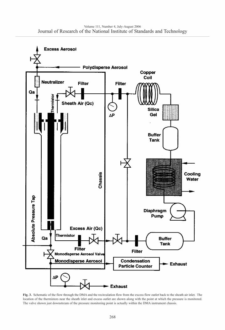
A schematic diagram of the recirculation systemis included in Fig. 3. Excess air leaves the classifier, pass-es through an adjustable needle valve and is then filteredthrough an ultra high efficiency pleated membranecartridge filter to remove any particles. From the filter,the flow enters a buffer tank. The tank is a brass cylinder40 cm long with a volume of 6 L and serves to dampenthe pulsations caused by the pump. After the buffer tank
are two diaphragm pumps connected in parallel. Theoperator can choose to have only one pump operate forlow flow rates, or have two pumps operate for higherflow rates. After the pumps, the flow travels through coilssubmerged in a water bath. Since the pumps heat the flow,the water bath is needed to reduce the temperature of theflow. The bath itself is cooled by a second set of coilscarrying tap water. After leaving the bath, the flow entersanother buffer tank, the same size as the first one,to further dampen the effects of the pump. From there theflow travels through a drier packed with silicagel to remove moisture from the flow. It then travelsthrough a coiled section that acts as a heat exchangerto allow the flow to reach room temperature. The condi-tioned flow is then split into two flows. Most of the flowis sent through another pleated membrane cartridge filter,to remove any residual particles, and then into the top ofthe classifier as the sheath flow. A small portion of theflow is diverted back into the recirculation system, join-ing the excess air as it leaves the classifier. Adjusting theby-pass needle valve provides a high resolution adjust-ment of the sheath flow. A key design feature is that thesheath flow equals the excess flow.
The second key feature is that the buffer tanks togeth-er with the filters and the drier greatly reduce the pressurefluctuations from the diaphragm pumps. Pressure fluctu-ations could be a problem because they would causemixing fluctuations, which, in turn, would affect theresolution of the size distribution measurement. A1.33 kPa (10 torr) differential pressure transducer with a1 ms time response was used to measure the pressurefluctuations in the excess flow line just outside the DMAchassis (Fig. 3). The pressure was recorded versus timefor the DMA operated at a nominal flow of 20 L/min withthe pump and also recorded for a steady flow of 20 L/minof nitrogen from a gas cylinder through the DMA withthe pump and recirculation system disconnected. Pressuremeasurements were also made just downstream ofthe pump. The frequency of the pump pressure puls-ations was about 29 Hz and the amplitude exceeded1333 Pa (10 torr). There was a small amplitude peak forthe buffered flow at about 29 Hz. The amplitude was atleast 270 times smaller than the pump amplitude. Someperiodicity was also observed for the steady flow case.The standard deviations of the pressure for the bufferedflow was about 5.1 Pa compared to about 3.7 Pa for thecylinder flow (cylinder). From a power spectral analysis(see Appendix B) it was found that all three caseshave peaks near 30 Hz and 60 Hz though much reducedin magnitude for the recirculations flow and cylinderflow.
Volume 111, Number 4, July-August 2006Journal of Research of the National Institute of Standards and Technology
267
Volume 111, Number 4, July-August 2006Journal of Research of the National Institute of Standards and Technology
268
Fig. 3. Schematic of the flow through the DMA and the recirculation flow from the excess flow outlet back to the sheath air inlet. Thelocation of the thermistors near the sheath inlet and excess outlet are shown along with the point at which the pressure is monitored.The valve shown just downstream of the pressure monitoring point is actually within the DMA instrument chassis.

There is also indirect evidence that the flow fluctua-tions were small. Flow fluctuations could cause mixingof the aerosol flow with the sheath flow. This wouldlead to a broadening of the size distribution. The nar-rowness of the size distribution of the SRM® 1963spheres (Fig. 5) described in Sec. 6.1 is evidence thatthe pulsations from the pump are not affecting the res-olution of the size distribution measurements.
4.4 Support Measurements of Pressure,Temperature, and Voltage
In addition to the recirculation system, equipmentwas added to the DMA measurement system to obtainaccurate pressure and temperature measurements. Thebarometric pressure is measured near the monodisperseexit (see Fig. 3) using a Mensor Corporation Model4011 digital pressure transducer containing an ionimplanted silicon strain gage. Thermistors provideaccurate temperature measurements at two locations inthe sheath flow: one is located in the upper sheath flowjust before it enters the DMA and the other is locatedafter the DMA exit. The thermistors are type CSPThermoprobes manufactured by ThermometricsIncorporated, with NIST traceable calibrations. Thepressure transducer and each of the thermistors providean updated digital output to the data acquisition systemat a rate of 1 Hz for continual monitoring of the envi-ronmental conditions used in the diameter calculations.
The appropriate pressure for computing the slipcorrection in Eq. (19) is the pressure within the DMA;thus the pressure drop across the exit slit must be deter-mined to correct the pressure reading made at themonodisperse outlet tube. To keep the pressure drop assmall as possible, the monodisperse aerosol valve wasalways fully open. The pressure drop inside the classi-fier was measured as a function of sheath flow as wellas aerosol flow through the classifier in a separate setof measurements [7]. Pressure measurements withvaried flows determined that the pressure differencewas a function of the aerosol flow rate only. Results forthe pressure drop measurements for a sheath flow of20 L/min are reported in Table 2.
The DMA voltage affects the measurement of theunknown particle size directly and also indirectlythrough the calibration measurement of the 100 nmSRM® 1963. Uncertainties in the voltage will affectthe calculated particle mobility as given in Eq. (2),which will in turn affect the measured particle diame-ter. A high voltage (1000 V to 10 000 V) calibrationfacility was set up to measure the voltage of the DMArod using a high voltage divider and a digital voltmeter.A Spellman HUD-100-1 precision resistor ladder wasused to step down the rod voltage. The output signalwas then measured using a Fluke Corporation 8060Adigital multimeter. It was critical that both the resistorladder and the volt meter be operated in a high imped-ance mode to obtain an accurate voltage. Both the resis-tor ladder and the multimeter have relative standarduncertainties of 0.05 % of the nominal reading over themeasurement range. The resistor loop provides DMArod voltage measurements with a relative combinedstandard uncertainty of ± 0.08 %.
4.5 Particle Concentration
The particle concentration is determined using amodel 3022A Condensation Particle Counter (CPC)manufactured by TSI Incorporated. The CPC detectsparticles by condensing supersaturated butanol vaporonto the particles to increase their size before they enterthe optical sensing zone where they are counted. TheCPC is capable of detecting particles of size 7 nm andlarger. The nominal number concentration is 100 cm–3
to 200 cm–3 for the 100 nm spheres produced by thepneumatic nebulizer and 200 cm–3 to 450 cm–3 for theelectrospray.
4.6 Data Acquisition
The data acquisition system consists of a desktopcomputer equipped with data acquisition boards andsoftware for communication with the instruments.Communication with the CPC and the electrostaticclassifier is accomplished via an RS-232 serial commu-nications port. Information from the digital pressuretransducer is collected using a National Instruments PCI6503 digital input/output board. Thermistors are con-nected to a National Instruments TBX 68T IsothermalTerminal Block, which relays the temperature informa-tion to a National Instruments 4351 PCI board. A cus-tomized data acquisition software program is used tocontrol the voltage setting of the DMA and sequencethrough a series of voltages with a fixed time interval foreach voltage. The number concentration, pressure, two
Volume 111, Number 4, July-August 2006Journal of Research of the National Institute of Standards and Technology
269
Table 2. Pressure drop inside classifier
Aerosol Flow Mean Pressure Standard DeviationRate, L / min Drop, Pa of Mean, Pa
0.5 2.9 0.31.0 8.7 0.42.0 26.0 0.3
thermistors, and voltage are recorded every second.Another custom program averages the data and providesthe averages and standard deviations for the quantitiesabove for each voltage setting. Both programs are writ-ten using National Instruments LabVIEW software.
5. Particle Characteristics and SamplePreparation
The 100 nm spheres were synthesized by DukeScientific Corporation using emulsion polymeriza-tion with styrene monomer. The bulk suspension wasdiluted with 18 MΩ deionized water filtered with a0.04 (µm) pore size filter. The sample mass fraction is0.5 % and the volume per sample is 5 mL. The massfraction of surfactant is 0.021 % and consisted ofsodium 1-dodecanesulfonate and 1-dodecanol. There isalso 0.006 % electrolyte remaining from the synthesis.There is no added preservative.
To prepare samples for analysis by the DMA, fivedrops of the suspension were diluted with 200 cm3 ofdeionized water filtered with an 0.2 µm pore size filter.The 100 nm SRM® 1963 samples were also preparedby diluting five drops of the SRM with 200 cm3 ofdeionized, filtered water. The nominal droplet size forboth of these samples and for the 60 nm spheres wasabout 0.040 cm–3.
The 60 nm spheres were synthesized by JSRCompany using emulsion polymerization with styrenemonomer. In this case the surfactant is synthesized intothe polymer itself as carboxyl groups so that no addi-tional surfactant is added.
One drop of the 60 nm PS spheres is added to the1 cm3 capsule filled with ammonium acetate solutionwith a conductivity of about 0.2 S/m (1 S ≡ 1/Ω). Thiscorresponds to about a 20 mmol/L solution. The ammo-nium acetate sublimates so that it does not contribute toa residue layer. The electrolyte/particles suspensionwas filtered with a 1.2 µm pore size filter to removelarge particles such as dust. This was done to minimizeparticle clogging of the electrospray capillary.
6. DMA Measurement Process
Two types of measurements were taken with theDMA. One measurement was the accurate determina-tion of the peak in the size distribution for the 60 nm or100 nm spheres and involved two steps. The first stepwas the calibration of the DMA using SRM® 1963.The second step was the actual determination of thepeak particle size using the DMA. The second DMAmeasurement involved determining the peak voltage
for a number of different sample bottles to test forhomogeneity of the samples. The method for determin-ing the peak voltage is discussed in this section, but theexperimental design and the analysis of variance to ver-ify the homogeneity of the different samples is present-ed in Sec. 7.
6.1 100 nm Spheres and SRM® 1963
The particle suspension was prepared as describedabove and the pneumatic aerosol generator was operat-ed at an aerosol flow of about 16 L/min with a 14 Laccumulator. The sheath flow was set to 20 L/min withthe DMA excess air valve fully open by adjustment ofthe two valves in the recirculation system. The aerosolflow was set to 0.5 L/min with the monodisperse valvefully open by adjusting the bypass valves controllingthe aerosol inlet flow. As discussed previously, thisapproach minimizes the pressure drop between theDMA column and the outlet flow. A preliminary scan ofnumber concentration versus voltage was taken todetermine the peak voltage and voltages correspondingto a decrease in the number concentration by about30 %, both above and below the peak. This correspond-ed to a voltage range of about 300 V for the 100 nmspheres and SRM® 1963, with peak voltage of about3500 V. These values allowed for 16 voltage channels,spaced by 20 V each, to be used in the data acquisitionprocess. The data acquisition was designed to collectnumber concentration once a second for 45 s at eachvoltage. Data was also collected every second for thepressure in the DMA and for the temperature of theDMA inlet and exhaust gas. It was found that the CPCreached a steady concentration within about 20 s of avoltage change. The average number concentration,average pressure, and average inlet and outlet tempera-ture were computed over the final 20 s of the 45 s dwelltime at a fixed voltage. The inlet and outlet tempera-tures typically differed by about 0.25 °C. The DMAtemperature was taken to be the numeric average of thetime averages for the inlet and outlet temperatures.
For the 100.7 nm SRM® 1963 particles, 16 voltage-steps were taken with 8 or 9 of these steps used indetermining the peak voltage. The voltage-stepsused to determine the peak had typically the rangeN/Npeak > 0.75, where Npeak is the highest number con-centration recorded by the CPC during a voltage scan.Two repeat data sets, taken on 20 September 2004, areshown in Fig. 4 along with the best fit cubic curvefor each measurement series. The best fit peaks are3501.2 V and 3502.0 V. If two more data points areadded extending the range to N/Npeak > 0.65, the peakvoltages decrease slightly to 3500.5 V and 3498.5 V.
Volume 111, Number 4, July-August 2006Journal of Research of the National Institute of Standards and Technology
270

The best fit cubic curve for the data is obtained usingthe proprietary KaleidaGraph nonlinear least squaressoftware. The peak in the curve is obtained by settingthe derivative of the cubic equation to zero. It wasfound that five significant figures in the coefficients ofthe cubic resulted in a numerical uncertainty of lessthan about ± 0.04 % for the voltage and particle sizepeaks obtained in this study.
Two repeat data sets for the 100 nm spheres are alsoshown in Fig. 4. It is seen that the 100 nm spheres havea slightly larger peak voltage and distribution width. Oneach of three days, three voltage scans were madeon the 100 nm spheres and four on the SRM® 1963particles.
As was discussed in Sec. 2.2, the measured peak inthe voltage for SRM® 1963 was compared withthe predicted voltage, using the known peak size of100.7 nm, the standard deviation of 2.0 nm and thetransfer function integral to compute the predicted peakvoltage. The flow rate was then adjusted from 20 L/min
to this value times the ratio of the voltages to get thecalibrated flow. For these two cases the corrected flowswere 21.153 L/min and 21.149 L/min.
The estimated size distribution, G(Dp), based on thefirst approximation method, is obtained from N(V)using Eq. (14). To obtain the diameter Dp correspon-ding to the voltage V requires two steps. First, themobility Zp corresponding to the voltage is computedusing Eq. (22) with the corrected flow rate. Then thediameter corresponding to the mobility is computediteratively using Eq. (2) together with the expressionsfor the slip correction, Eq. (18), and the expression forthe mean free path, Eq. (20). The size distributions cor-responding to the plots of N(V) in Fig. 4 are plotted inFig. 5. The peak diameters based on the cubic fits are101.53 nm and 101.63 nm. In the certification measure-ments, the 100.1 nm diameter point was not includedand the corresponding peak diameters were 101.70 nmand 101.68 nm. This represents a worst case in terms offitting because of the asymmetry in G(Dp) between the
Volume 111, Number 4, July-August 2006Journal of Research of the National Institute of Standards and Technology
271
Fig. 4. The number concentration normalized by the concentration at the peak is plotted versus voltage for two repeatmeasurements for the 100 nm spheres and for SRM®1963, 100.7 nm spheres used to calibrate the DMA. SRM run c(solid circle), g (open circle); 100 nm run b (solid square), d (open square) taken on 20 September 2004. Curves denotebest fit cubics for the individual measurements (dashed curve fit for solid symbols; solid curve for open symbols).

smallest and largest diameters in the fitting range,whether or not the point at 100.1 nm is included.However, even in this worst case, the difference in thetwo estimates is 0.17 % in one case and 0.07 % in theother.
The peak sizes of 100.73 nm and 100.71 nm forSRM® 1963 demonstrate the consistency of the cali-bration procedure, which adjusted the value of thesheath flow so that the measured peak in the voltageplot would equal the value predicted assuming aGaussian size distribution with a peak at 100.7 nm.Figure 5 also provides a comparison of the measuredsize distribution and Gaussian distributions with a num-ber mean size of 100.7 nm and standard deviations of2.0 nm and of 1.8 nm. The agreement appears to beslightly better for the narrower Gaussian distribution.The value of the standard deviation obtained by trans-mission electron microscopy was 2.0 nm.
The 100 nm spheres were also measured over widersize ranges to better define the full distribution and
to see if the multiply charged dimers or trimers wereinterfering in the size measurement. A voltage scanfrom about 3100 V to 3900 V showed an almost 10 fold variation in the concentration as shown in Fig. 6. Theresults are plotted for both 1 drop and 6 drops of theparticle suspension diluted in 200 mL of particle freedeionized water. The six-fold increase in particlesresulted in only about a doubling of the concentration.There appear to be two outlier data points around3350 V and 3450 V in run F (Fig. 6), which might haveresulted from the voltage failing to increase at theproper time. Subsequent observations made whileobserving the DMA display along with the computerdisplay demonstrated that this would happen at infre-quent intervals, perhaps once every two or three scans.
The reduced number distributions for the 100 nmparticles, plotted in Fig. 7, agree well up to the peak.For particle diameters beyond the peak, a slight off-setin the distributions is apparent for particle diameters that increases to about 0.3 nm for the largest sizes
Volume 111, Number 4, July-August 2006Journal of Research of the National Institute of Standards and Technology
272
Fig. 5. The number size distribution normalized by the peak in the distribution is plotted versus diameter for the100 nm spheres and for the SRM®1963 spheres for the same data as Fig. 4. The short and long dashed curve corre-sponds to the Gaussian size distribution of SRM® 1963 with the certified number mean diameter of 100.7 nm andstandard deviation of 1.8 nm (narrower curve) and 2.0 nm.

Volume 111, Number 4, July-August 2006Journal of Research of the National Institute of Standards and Technology
273
Fig. 6. Plot of number concentration versus voltage for the full range of the size distribution.Displayed data is for 100 nm run d (open circle, left axis) with 1 drop per 200 cm3 and run f (solidcircle, right axis) with 6 drops per 200 cm3. Data were taken on 14 October 2004.
Fig. 7. The normalized number size distribution is plotted for the same data set as Fig. 6. Forcomparison a Gaussian distribution with a mean 101.5 nm and a standard deviation of 2.5 nm isplotted as a dashed curve.
measured. For comparison purposes, a Gaussian sizedistribution with a peak size of 101.50 nm and a standard deviation of 2.5 nm is also plotted. The Gaussian over-laps the two data sets for the reduced G(Dp) > 0.4. ForG(Dp) < 0.4, the measured values are asymmetric at thesmaller size particles.
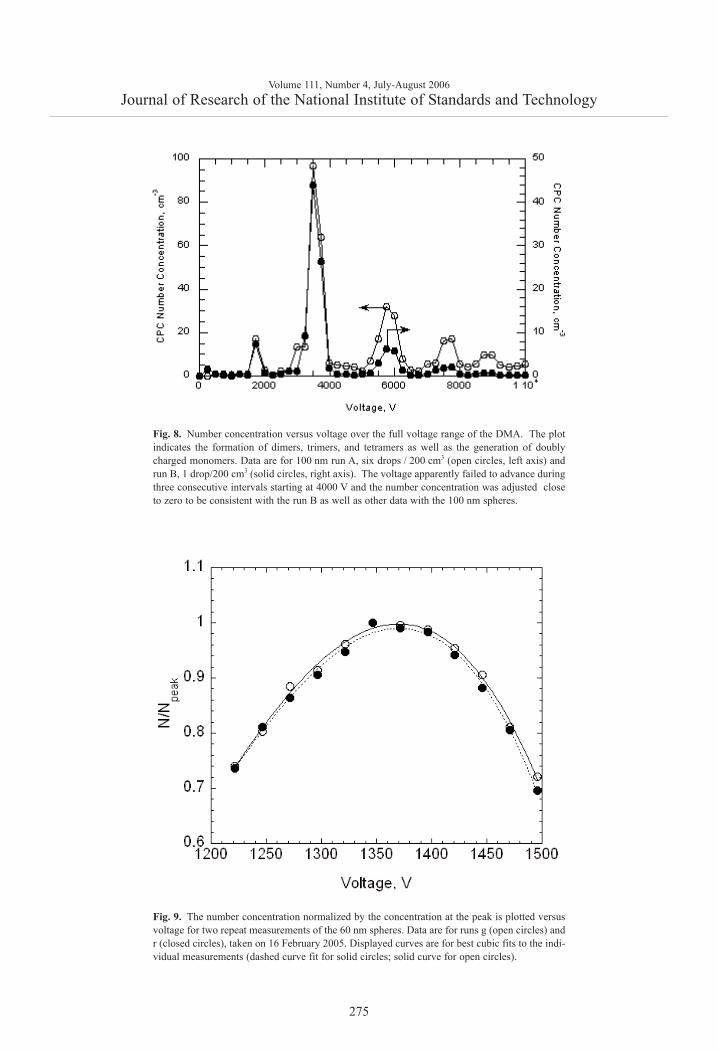
Two scans were made in 250 V increments fromessentially zero to 10 000 V for the two particle concen-trations used previously. As seen in Fig. 8, there is aprominent peak from the singly charged 100 nm spheresand a number of other peaks resulting from doublycharged spheres and from sphere aggregates includingdimers, trimers, and tetramers. We adopt the terminolo-gy of mass spectrometry, in which the singlets, doublets,...multiplets always refer to the charge, and monomer,dimer, ...multimer always refer to the number of primaryparticles in an aggregate. Then a singly charged dimerand a doubly charged trimer become a singlet dimer anda doublet trimer. There is a possibility that multiplet mul-timers will have mobilities overlapping that of the singletmonomer. The typical analysis region for sizing the 100nm spheres was from 3450 V to 3650 V. If there weresinglet trimers with voltage in the range of 6900 V to7300 V, then the corresponding doublet trimers wouldrange from 3450 V to 3650 V. For run A the particle con-centration measured at 6990 V, 7240 V, and 7490 were(5.8, 6.0, and 16.5) cm–3, respectively, compared to apeak concentration of 97 cm–3. The possible impact ofdoublet trimers on the sizing of the 100 nm spheres willbe discussed in Sec. 8.3.7. Over the voltage range corre-sponding to the full width of the 100 nm size distributionshown in Fig. 7, 3170 V to 3900 V, there would be aslight contribution from the doublet dimer in the smallparticle size region and from the doublet trimer in thepeak particle size region.
6.2 60 nm Spheres
For the 60 nm spheres, the electrospray generator wasused with a 2 L/min output followed by a 1 L accumula-tor. The measurement approach was similar to that usedfor the 100 nm spheres except that two 45 s scans weremade at the start of the experiment at the peak voltageand then again at the end of the experiment. These addi-tional measurements were to correct for instrumentdrift over the 15 min period of data collection. Previousdiagnostic measurements indicated that the drift wasmuch larger in this case than for the pneumatic nebulizer.Also, after finding evidence of an infrequent failure ofthe DMA voltage to be changed at the proper time, thecorrect voltage was verified/corrected at each time incre-ment for the 60 nm spheres.
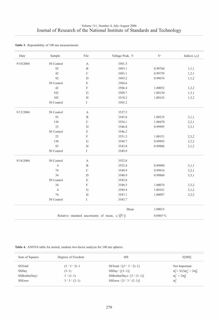
The nominal peak voltage for the 60 nm spheres was1370 V, with the voltage range extended over 350 V in15 steps of 25 V each. The value of N/Np was about 0.6at the largest and smallest voltage. The relatively largesteps were required because of the broadness of the sizedistribution and the lower stability of the generator com-pared to the pneumatic generator. In this case, about 12data points were fitted over the range of N/Np > 0.75 todetermine the peak voltage. The results and cubic fits forruns F and G, taken on 16 February 2005, are shown inFig. 9.
The electrospray was also used with the SRM® 1963spheres for the calibration of the DMA. In this case,25 V increments were chosen rather than the 20 V incre-ment used with the pneumatic generator. Otherwise thecalibration was identical to the procedure describedabove. The results for the size distribution G(Dp) areplotted in Fig. 10. The best fit peak diameters over therange N/Np > 0.75 are 60.62 nm for run F and 60.52 nmfor G. Removing the lowest two points so that the fit isover the range greater than 0.80 results in a 0.03 nmdecrease in the peak diameter for F and a 0.06 nmincrease for G.
As was done for the 100 nm particles, data were alsocollected over a larger range in voltage to obtain the fullsize distribution. The results, plotted in Fig. 11, indicatea plateau in the low voltage region. The doubletmonomer would be classified at a voltage of about675 V, which overlaps with the plateau in the smallparticle size of the size distribution. Based on the relativecharging probability of a doublet monomer to a singletmonomer [16], the estimated particle number concentra-tion of 18 cm–3, of the total of 48 particles cm–3, would bedoublet monomers. A logarithmic plot of the data over awider range is needed to depict the very low contributionof dimers and trimers and is shown in Fig. 12. The sin-glet dimer voltage is about 2200 V corresponding to theplateau region in Fig. 12. The ratio of singlet monomersto singlet dimers is approximately 3 × 10⁻³. So in thiscase, the contribution from multimers can be ignored.
The number distribution G(Dp) corresponding to thevoltage distribution in Fig. 11 is plotted in Fig. 13. It isseen that a Gaussian distribution with a peak of 60.5 nmand a width of 4.9 nm has the same width as the meas-ured distribution for G(Dp)/ G(Dp)peak > 0.5, but themeasured distribution is noticeably asymmetric towardsthe small particle sizes. Also one set of results is includ-ed in Fig. 13 where an attempt has been made to subtractthe contribution of the doubly charged monomer concen-tration using the estimated charging probability. Thecorrected monomer distribution does not have a plateau.
Volume 111, Number 4, July-August 2006Journal of Research of the National Institute of Standards and Technology
274
Volume 111, Number 4, July-August 2006Journal of Research of the National Institute of Standards and Technology
275
Fig. 8. Number concentration versus voltage over the full voltage range of the DMA. The plotindicates the formation of dimers, trimers, and tetramers as well as the generation of doublycharged monomers. Data are for 100 nm run A, six drops / 200 cm3 (open circles, left axis) andrun B, 1 drop/200 cm3 (solid circles, right axis). The voltage apparently failed to advance duringthree consecutive intervals starting at 4000 V and the number concentration was adjusted closeto zero to be consistent with the run B as well as other data with the 100 nm spheres.
Fig. 9. The number concentration normalized by the concentration at the peak is plotted versusvoltage for two repeat measurements of the 60 nm spheres. Data are for runs g (open circles) andr (closed circles), taken on 16 February 2005. Displayed curves are for best cubic fits to the indi-vidual measurements (dashed curve fit for solid circles; solid curve for open circles).

Volume 111, Number 4, July-August 2006Journal of Research of the National Institute of Standards and Technology
276
Fig. 10. The number size distribution normalized by the peak in the distribution is plottedversus diameter for the same two 60 nm data sets as in Fig. 9.
Fig. 11. Number concentration versus voltage over the full size distribution of the 60 nm spheres.Data are for runs b (open circles) and c (x’s), taken on 25 February 2005.

Volume 111, Number 4, July-August 2006Journal of Research of the National Institute of Standards and Technology
277
Fig. 12. Data from Fig. 11 plotted using a logarithmic scale to show the much lower dimerconcentration compared to the pneumatic aerosol generator.
Fig. 13. Number size distribution versus diameter based on the data from Fig. 11. The data iscompared to a Gaussian with mean of 60.5 nm and standard deviation of 4.9 nm (solid curve).The cross symbols (+) denote data from run c, corrected for the contribution from doubletmonomers (doubly charged monomer).

7. Experimental Design and StatisticalAnalysis for Homogeneity, BestEstimate of Peak Diameter, andRepeatability Uncertainty
The experimental design for testing the homogeneityof the 60 nm and 100 nm samples, for determining thebest estimate of the peak diameters, and for determiningthe uncertainty associated with repeatability is presented.The repeatability uncertainty, which is a so-called TypeA uncertainty, is needed for computing the overall sizinguncertainty by combining with the Type B uncertaintydiscussed in the next section. The Type A uncertaintiesare those computed by statistical methods while the TypeB uncertainties are computed by other means and aregenerally based on scientific judgment using all the rele-vant information available [4]. The relative uncertainty,which is the uncertainty divided by the mean value, willbe used throughout this paper. The statistical analysismodel is described in his section and the results of theanalysis of variance (ANOVA) are presented.
7.1 Homogeneity Test—100 nm Spheres
The purpose of the homogeneity test was to verify atthe 95 % confidence level that each bottle has the samepeak size. The following experimental design was used.Nine bottles were selected at random from a lot of 150bottles. On each of three different days, three bottleswere assigned and two repeat measurements of peakvoltage were performed from each bottle, for a total ofeighteen measurements. The measurement plan is shownin Table 3. This sampling design is called a nested design[22], with bottles nested within a day, as opposed to a fullfactorial design, which would require that all nine bottlesbe measured each day. Taking this many measurementstogether with the control measurements was not feasible.
The procedure for determining the peak voltage wasdiscussed in Sec. 6. The voltage peak is closely related tothe peak in the particle diameter distribution. From theuncertainty in the peak voltage, the uncertainty in theparticle diameter can be computed as discussed in thelast part of this section.
To compensate for possible instrument drift within aday, the peak voltage of a control sample is measured, atthe beginning of the series of measurements, at the mid-point, and at the end of the measurements. The peak volt-age for the first two measurements, 92B and 42C asshown in Table 4, are divided by the peak voltage for theAth run of the control sample, which was labeled as the50th sample. The next two sample measurements aredivided by the middle control and the last two measure-ments by the last control. The same methodology isfollowed on the other two days. Causes of drift
include changes in the ambient temperature and pres-sure.
To test for homogeneity, a two-factor analysis of vari-ance was run with the factors being nested and random.The two random factors are: the day to day effects whichare indexed by i and the bottle to bottle effects indexedby j. A random day effect means that if the measurementswere performed on any day, observed daily fluctuationswould look like a normal distribution. Replicate meas-urements are identified by the index k. Each of the 18measured values of the normalized voltage are, there-fore, denoted by Vrijk, i = 1,2,3, j = 1,2,3, k = 1,2.
In a nested design analysis of variance model, thenormalized voltages are assumed to be given by:
(22)where:
µ is a constant representing the component of peakvoltage common to all measurements, whichcan also be thought of as the true value of thepeak voltage, and is estimated by V—r..., the aver- age of the 18 measurements of Vri j k ,where eachdot represents an average over an index.
αi are N(0,σα2), which is an abbreviation for nor-
mally distributed random variables with mean zero and variance σα
2. The quantity αi measuresthe random differences due to day to day variation.
βj(i) are N(0,σβ2 ) random variables measuring varia-
tions from to bottle to bottle. The parenthesesaround the index i signify that the j index cor-responds to a fixed day (nested within a day).
εk(ij) are N(0,σε2 ) random variables incorporating all
other variation. The parentheses around i j signi-fy that the k index corresponds to a fixed dayand a fixed bottle.
Analysis of variance is based on the fact that the totalsum of squares (SS) can be partitioned as follows:
(23)
where,
(24)
Each of the individual sums of squares has associateddegrees of freedom and expectations given in Table 4.
Volume 111, Number 4, July-August 2006Journal of Research of the National Institute of Standards and Technology
278
.. ( ) ( ) ,i j k i j i k i jVr µ α β ε= + + +
( ) ( )22
... .. ...3 2ijk ii j k i
Vr Vr Vr Vr− = ⋅ −∑∑∑ ∑
( ) ( )22
. .. .2 ,ij i ijk iji j i j k
Vr Vr Vr Vr+ − + −∑∑ ∑∑∑( ) ,SSTotal SSDay SSBottle Day SSError= + +
... ... ..., /18 ,i j ki j k
Vr Vr Vr Vr= → =∑∑∑
. ..1 1, and .2 6ij ijk i ijk
k j kVr Vr Vr Vr= =∑ ∑∑
Volume 111, Number 4, July-August 2006Journal of Research of the National Institute of Standards and Technology
279
Table 3. Repeatability of 100 nm measurements
Date Sample File Voltage Peak, V Vr Indices i,j,k
9/10/2004 50 Control A 3501.592 B 3493.1 0.99760 1,1,142 C 3493.1 0.99759 1,2,192 D 3493.2 0.99676 1,1,2
50 Control E 3504.642 F 3506.4 1.00052 1,2,2
102 G 3509.7 1.00130 1,3,1102 H 3510.2 1.00143 1,3,2
50 Control I 3505.2
9/13/2004 50 Control A 3537.593 B 3545.8 1.00235 2,1,1
130 C 3554.1 1.00470 2,2,125 D 3546.0 0.99995 2,3,1
50 Control E 3546.225 F 3551.5 1.00151 2,3,2
130 G 3549.7 0.99993 2,2,293 H 3543.0 0.99806 2,1,2
50 Control I 3549.9
9/14/2004 50 Control A 3552.84 B 3552.4 0.99989 3,1,1
74 C 3549.9 0.99916 3,2,134 D 3540.9 0.99860 3,3,1
50 Control E 3545.834 F 3548.5 1.00074 3,3,24 G 3549.4 1.00161 3,1,2
74 H 3547.1 1.00097 3,2,250 Control I 3543.7
Mean 1.00015
Relative standard uncertainty of mean, 0.0465 %
Table 4. ANOVA table for nested, random two-factor analysis for 100 nm spheres
Sum of Squares Degrees of Freedom MS E[MS]
SSTotal (3 · 3 · 2)–1 SSTotal / [(3 · 3 · 2)–1] Not ImportantSSDay (3–1) SSDay / [(3–1)] σε
2+ 3(2)σα2 + 2σβ
2
SSBottle(Day) 3 · (3–1) SSBottle(Day) / [3 · (3–1)] σε2 + 2σβ
2
SSError 3 · 3 · (2–1) SSError / [3 · 3 · (2–1)] σε2
( )Aru Vr
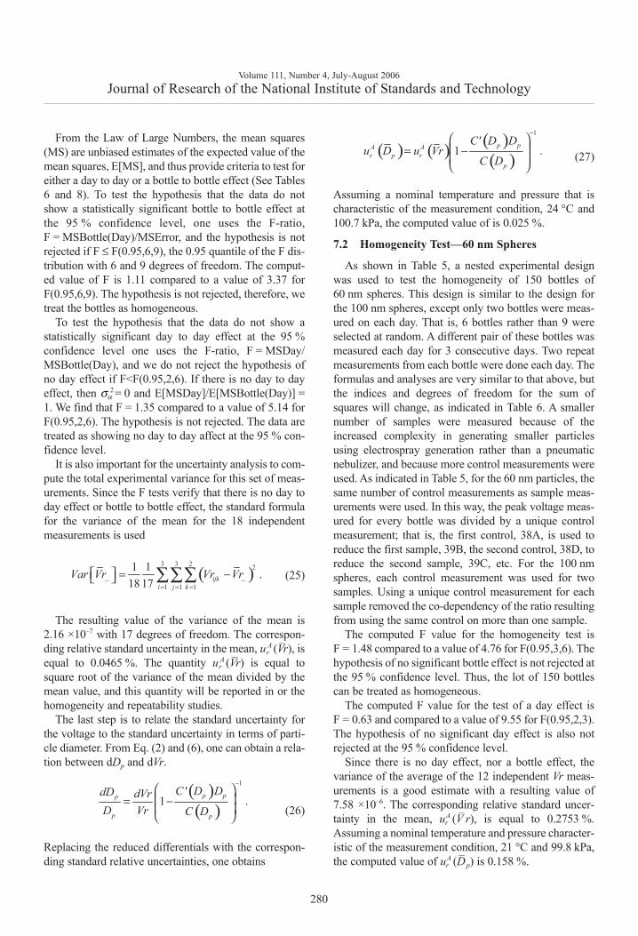
From the Law of Large Numbers, the mean squares(MS) are unbiased estimates of the expected value of themean squares, E[MS], and thus provide criteria to test foreither a day to day or a bottle to bottle effect (See Tables6 and 8). To test the hypothesis that the data do notshow a statistically significant bottle to bottle effect atthe 95 % confidence level, one uses the F-ratio,F = MSBottle(Day)/MSError, and the hypothesis is notrejected if F ≤ F(0.95,6,9), the 0.95 quantile of the F dis-tribution with 6 and 9 degrees of freedom. The comput-ed value of F is 1.11 compared to a value of 3.37 forF(0.95,6,9). The hypothesis is not rejected, therefore, wetreat the bottles as homogeneous.
To test the hypothesis that the data do not show astatistically significant day to day effect at the 95 %confidence level one uses the F-ratio, F = MSDay/MSBottle(Day), and we do not reject the hypothesis ofno day effect if F<F(0.95,2,6). If there is no day to dayeffect, then σα
2= 0 and E[MSDay]/E[MSBottle(Day)] =1. We find that F = 1.35 compared to a value of 5.14 forF(0.95,2,6). The hypothesis is not rejected. The data aretreated as showing no day to day affect at the 95 % con-fidence level.
It is also important for the uncertainty analysis to com-pute the total experimental variance for this set of meas-urements. Since the F tests verify that there is no day today effect or bottle to bottle effect, the standard formulafor the variance of the mean for the 18 independentmeasurements is used
(25)
The resulting value of the variance of the mean is2.16 ×10–7 with 17 degrees of freedom. The correspon-ding relative standard uncertainty in the mean, ur
A (V–r), isequal to 0.0465 %. The quantity ur
A (V–r) is equal tosquare root of the variance of the mean divided by themean value, and this quantity will be reported in or thehomogeneity and repeatability studies.
The last step is to relate the standard uncertainty forthe voltage to the standard uncertainty in terms of parti-cle diameter. From Eq. (2) and (6), one can obtain a rela-tion between dDp and dVr.
(26)
Replacing the reduced differentials with the correspon-ding standard relative uncertainties, one obtains
(27)
Assuming a nominal temperature and pressure that ischaracteristic of the measurement condition, 24 °C and100.7 kPa, the computed value of is 0.025 %.
7.2 Homogeneity Test—60 nm Spheres
As shown in Table 5, a nested experimental designwas used to test the homogeneity of 150 bottles of60 nm spheres. This design is similar to the design forthe 100 nm spheres, except only two bottles were meas-ured on each day. That is, 6 bottles rather than 9 wereselected at random. A different pair of these bottles wasmeasured each day for 3 consecutive days. Two repeatmeasurements from each bottle were done each day. Theformulas and analyses are very similar to that above, butthe indices and degrees of freedom for the sum ofsquares will change, as indicated in Table 6. A smallernumber of samples were measured because of theincreased complexity in generating smaller particlesusing electrospray generation rather than a pneumaticnebulizer, and because more control measurements wereused. As indicated in Table 5, for the 60 nm particles, thesame number of control measurements as sample meas-urements were used. In this way, the peak voltage meas-ured for every bottle was divided by a unique controlmeasurement; that is, the first control, 38A, is used toreduce the first sample, 39B, the second control, 38D, toreduce the second sample, 39C, etc. For the 100 nmspheres, each control measurement was used for twosamples. Using a unique control measurement for eachsample removed the co-dependency of the ratio resultingfrom using the same control on more than one sample.
The computed F value for the homogeneity test isF = 1.48 compared to a value of 4.76 for F(0.95,3,6). Thehypothesis of no significant bottle effect is not rejected atthe 95 % confidence level. Thus, the lot of 150 bottlescan be treated as homogeneous.
The computed F value for the test of a day effect isF = 0.63 and compared to a value of 9.55 for F(0.95,2,3).The hypothesis of no significant day effect is also notrejected at the 95 % confidence level.
Since there is no day effect, nor a bottle effect, thevariance of the average of the 12 independent Vr meas-urements is a good estimate with a resulting value of7.58 ×10–6. The corresponding relative standard uncer-tainty in the mean, ur
A (V–r), is equal to 0.2753 %.Assuming a nominal temperature and pressure character-istic of the measurement condition, 21 °C and 99.8 kPa,the computed value of ur
A (D– p) is 0.158 %.
280
Volume 111, Number 4, July-August 2006Journal of Research of the National Institute of Standards and Technology
( )3 3 2 2
... ...1 1 1
1 1 .18 17 ijk
i j kVar Vr Vr Vr
= = =
= − ∑∑∑
( )( )
1'
1 .p pp
p p
C D DdD dVrD Vr C D
− = −
( ) ( ) ( )( )
1
1 .p pA Ar p r
p
C' D Du D u Vr
C D
− = −
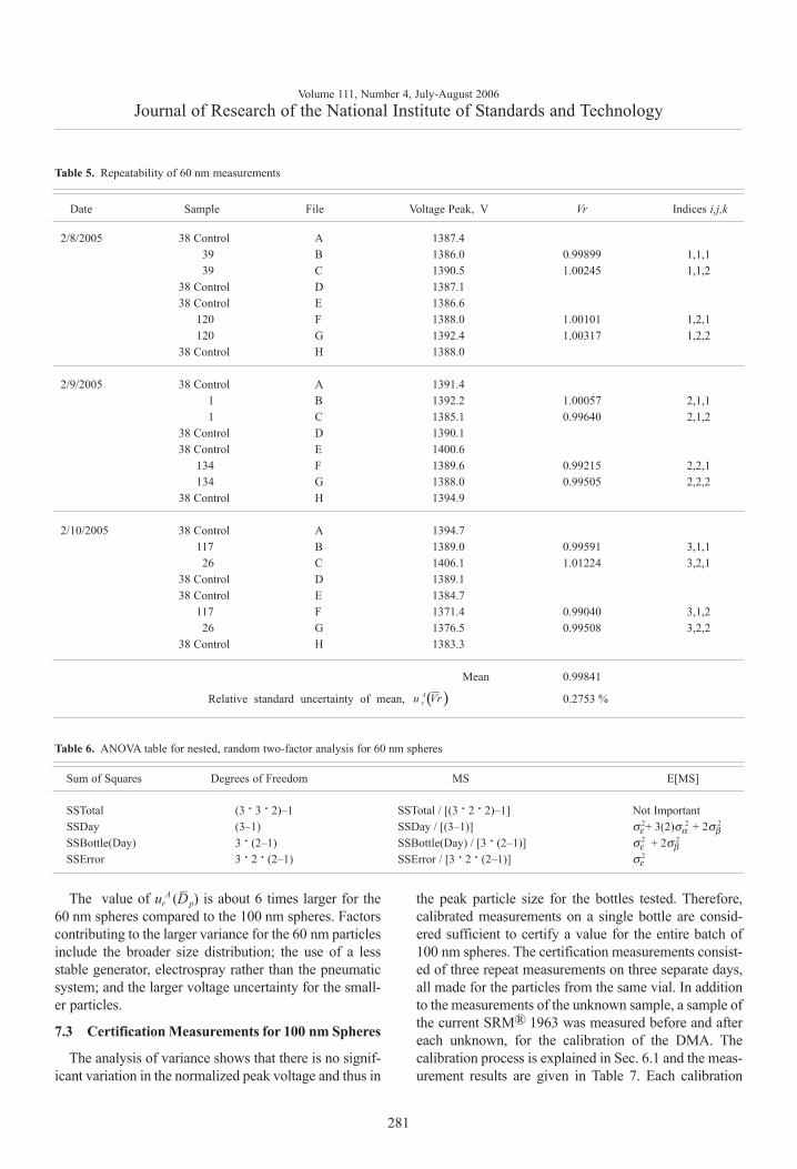
The value of urA (D– p) is about 6 times larger for the
60 nm spheres compared to the 100 nm spheres. Factorscontributing to the larger variance for the 60 nm particlesinclude the broader size distribution; the use of a lessstable generator, electrospray rather than the pneumaticsystem; and the larger voltage uncertainty for the small-er particles.
7.3 Certification Measurements for 100 nm Spheres
The analysis of variance shows that there is no signif-icant variation in the normalized peak voltage and thus in
the peak particle size for the bottles tested. Therefore,calibrated measurements on a single bottle are consid-ered sufficient to certify a value for the entire batch of100 nm spheres. The certification measurements consist-ed of three repeat measurements on three separate days,all made for the particles from the same vial. In additionto the measurements of the unknown sample, a sample ofthe current SRM® 1963 was measured before and aftereach unknown, for the calibration of the DMA. Thecalibration process is explained in Sec. 6.1 and the meas-urement results are given in Table 7. Each calibration
281
Volume 111, Number 4, July-August 2006Journal of Research of the National Institute of Standards and Technology
Table 5. Repeatability of 60 nm measurements
Date Sample File Voltage Peak, V Vr Indices i,j,k
2/8/2005 38 Control A 1387.439 B 1386.0 0.99899 1,1,139 C 1390.5 1.00245 1,1,2
38 Control D 1387.138 Control E 1386.6
120 F 1388.0 1.00101 1,2,1120 G 1392.4 1.00317 1,2,2
38 Control H 1388.0
2/9/2005 38 Control A 1391.41 B 1392.2 1.00057 2,1,11 C 1385.1 0.99640 2,1,2
38 Control D 1390.138 Control E 1400.6
134 F 1389.6 0.99215 2,2,1134 G 1388.0 0.99505 2,2,2
38 Control H 1394.9
2/10/2005 38 Control A 1394.7117 B 1389.0 0.99591 3,1,126 C 1406.1 1.01224 3,2,1
38 Control D 1389.138 Control E 1384.7
117 F 1371.4 0.99040 3,1,226 G 1376.5 0.99508 3,2,2
38 Control H 1383.3
Mean 0.99841
Relative standard uncertainty of mean, 0.2753 %( )Aru Vr
Table 6. ANOVA table for nested, random two-factor analysis for 60 nm spheres
Sum of Squares Degrees of Freedom MS E[MS]
SSTotal (3 · 3 · 2)–1 SSTotal / [(3 · 2 · 2)–1] Not ImportantSSDay (3–1) SSDay / [(3–1)] σε
2+ 3(2)σα2 + 2σβ
2
SSBottle(Day) 3 · (2–1) SSBottle(Day) / [3 · (2–1)] σε2 + 2σβ
2
SSError 3 · 2 · (2–1) SSError / [3 · 2 · (2–1)] σε2

measurement was associated with only a single measure-ment of the 100 nm spheres to avoid co-dependency ofthe results.
The notation for the particle diameter measurements isDp(ij), where the index i (i = 1, 2, 3) is over days and theindex j (j = 1, 2, 3) is over repetitions within a day. Theone factor statistical model with random effects is givenby:
(28)where:
µ.. is a constant representing the component of thepeak diameter common to all measurements andis estimated by D– p(..), the average of all twelvemeasurements of Dp(ij) where each dot repre-sents an average over an index.
αi are N(0,σα2) measuring differences due to day to
day variation.
ε ij are N(0,σε2 ) random variables incorporating mea-
surement repeatability and all other variation.
The ANOVA model is given in Table 8. The comput-ed F value for the test of a day effect is F = 1.28 com-pared to a value of 5.14 for F(0.95,2,6). The hypothesisof no significant day effect is not rejected at the 95%confidence level.
Since there is no day effect, the variance can be esti-mated as the variance of the mean of the nine independ-ent measurements of the peak diameter
(29)
The resulting value of the variance is 9.309×10⁻⁴ with 8degrees of freedom and the value of ur
A (D– p) = 0.0300 %.
282
Volume 111, Number 4, July-August 2006Journal of Research of the National Institute of Standards and Technology
( ) ,p i ijD ij µ α ε= + +
( )( ) ( ) ( )( )3 3 2
.. ..1 1
1 1 .9 8p p p
i jVar D D ij D
= =
= − ∑∑
Table 7. Particle diameter, adjusted flow, T, and P for 100 nm spheres accurate sizing measurements
Date Sample Diameter, nm Flow, L/min* T(avg), °C Pressure, kPa
9/16/2004 SRM1963 21.235 24.187 100.170B 101.54 21.235 24.234 100.162
SRM1963 21.234 24.251 100.152D 101.48 21.210 24.269 100.136
SRM1963 21.185 24.267 100.112F 101.57 21.223 24.295 100.101
SRM1963 21.223 24.314 100.093
9/20/2004 SRM1963 21.102 24.025 101.130B 101.70 21.102 24.027 101.106
SRM1963 21.153 24.060 101.092D 101.46 21.126 24.102 101.088
SRM1963 21.099 24.139 101.077F 101.71 21.149 24.190 101.053
SRM1963 21.149 24.215 101.032
9/22/2004 SRM1963 21.064 24.191 100.736B 101.59 21.064 24.205 100.732
SRM1963 21.073 24.196 100.718D 101.64 21.061 24.191 100.697
SRM1963 21.048 24.183 100.686F 101.67 21.084 24.155 100.669
SRM1963 21.084 24.189 100.660
Mean Diameter 101.60Relative standard deviation
0.0300 %
* The values in bold are based on the calibration data and are used to compute the peak diameter.
( )of mean, Ar pu D

7.4 Certification Measurements for 60 nm Spheres
The analysis of variance shows that there is no signif-icant variation in the normalized peak voltage for the60 nm spheres and thus in the peak particle size due tothe bottles tested. Therefore, calibrated measurements ona single vial are considered sufficient to certify a valuefor the entire batch of the 60 nm spheres.
The experimental design for the 60 nm sphere meas-urement was similar to that of the 100 nm spheres. Themeasurement results for the diameter at the peak of thenumber distribution are given in Table 9 and the ANOVAmodel for this experimental design is given in Table 10.The major difference from the 100 nm measurements isthat four measurements were made each day instead ofthree. The other change is a slight rearrangement ofthe measurement sequence for the calibration spheres,allowing an additional repeat measurement based onthe same number of calibration measurements. For the100 nm spheres, the first and last calibrations of the daywere used with the first and last samples measured. Theaverage of the second and third calibration was used forthe middle measurement. For the 60 nm spheres, the firstmeasurement used the first calibration, the second meas-urement used the second calibration, etc. In neither casewas a calibration measurement used in normalizing morethan one measurement to avoid codependency.
The computed F value for the test of a day effect isF = 2.57 compared to a value of 4.46 for F(0.95,2,8). Thehypothesis of no significant day effect is accepted at the95 % confidence level. Since there is no day effect, thevariance can be estimated as the variance of the mean ofthe twelve independent measurements of the peak dia-meter. The resulting value of the variance is 13.20 ×10⁻⁴
with 11 degrees of freedom and the value of urA(D–p) =
0.0659 %.The Type A statistical results are summarized in
Table 11 for the four sets of experiments. It is seen thatfor both particle sizes the homogeneity experimentsand the certification measurements give relative standarduncertainties for the peak diameter within a factor
of three. Also, in both cases, the uncertainties were atleast a factor of two smaller for the 100 nm spheres com-pared to the 60 nm spheres. As discussed above, themajor contributors to the larger uncertainty for the60 nm spheres are thought to be the broader size distri-bution and the less steady operation of the electro-spray generator compared to the pneumatic aerosolgenerator.
8. Type B Uncertainties/Propagation andExpanded Uncertainty
This section focuses on the uncertainties based onscientific judgment and on results from other studies.First, the key uncertainties are identified and then theireffect on the uncertainty in particle size is obtained viapropagation of uncertainty. Finally, the Type B uncer-tainty computed in this section is combined with theType A in the previous section and a coverage factorestimated to give the expanded uncertainty, whichcorresponds to the 95 % confidence interval.
8.1 Uncertainty in Key Quantities
The values of the quantities needed for computingthe peak particle diameter together with their uncertain-ties are summarized in Table 12. The methodology forestimating these uncertainties is given below.
8.1.1 Pressure
The barometric pressure is measured using a MensorCorporation Model 4011 digital pressure transducercontaining an ion implanted silicon strain gage. Thepressure transducer has a NIST traceable calibrationwith a relative combined standard uncertainty of± 0.010 % over the range of 70 kPa to 140 kPa and aresolution of 0.0013 kPa (see Fig. 2). The pressure ismeasured in the monodisperse aerosol tube before thevalve. The pressure drop across the monodisperseaerosol outlet slit at a monodisperse aerosol flowof 0.5 L/min was 3 Pa, which is small compared to themeasurement uncertainty and is not corrected for.
283
Volume 111, Number 4, July-August 2006Journal of Research of the National Institute of Standards and Technology
Table 8. ANOVA table for one factor analysis with random effects for 100 nm spheres
Sum of Squares Degrees of Freedom MS E[MS]
SSTotal (3 · 3 )–1 SSTotal / [(3 · 3 )–1] Not ImportantSSDay (3–1) SSDay / [(3–1)] σε
2+ 3σα2
SSError 3 · (3–1) SSError / [3 · (3–1)] σε2

284
Volume 111, Number 4, July-August 2006Journal of Research of the National Institute of Standards and Technology
Table 9. Particle diameter, adjusted flow, T, and P for 60 nm spheres accurate sizing measurements
Test Date Test ID Diameter, nm Flow, L/min* T(avg), °C Pressure, kPa
2/15/2005 SRM1963 20.377 20.590 100.168B 60.451 20.377 20.713 100.140C 60.438 20.398 20.731 100.117
SRM1963 20.398 20.744 100.100SRM1963 20.411 20.739 100.108
F 60.435 20.411 20.707 100.084G 60.408 20.417 20.672 100.077
SRM1963 20.417 20.649 100.066
2/16/2005 SRM1963 20.472 20.465 99.020B 60.525 20.472 20.491 99.073C 60.641 20.427 20.523 99.087
SRM1963 20.427 20.563 99.164SRM1963 20.413 20.588 99.229
F 60.615 20.413 20.638 99.257G 60.518 20.457 20.680 99.247
SRM1963 20.457 20.746 99.396
2/18/2005 SRM1963 20.307 20.483 100.322B 60.155 20.307 20.556 100.332C 60.567 20.306 20.611 100.354
SRM1963 20.306 20.651 100.396SRM1963 20.325 20.664 100.429
F 60.277 20.325 20.649 100.488G 60.516 20.322 20.679 100.498
SRM1963 20.322 20.618 100.498
Mean Diameter 60.462Relative standard deviation
0.0659 %
* The values in bold are based on the calibration data and are used to compute the peak diameter.
( )of mean, Ar pu D
Table 10. ANOVA table for one factor analysis with random effects for 60 nm spheres
Sum of Squares Degrees of Freedom MS E[MS]
SSTotal (4 · 3 )–1 SSTotal / [(4 · 3 )–1] Not ImportantSSDay (3–1) SSDay / [(3–1)] σε
2+ 3σα2
SSError 4 · (3–1) SSError / [4 · (3–1)] σε2
Table 11. Summary of Type A statistical analysis for particle sizing uncertainty
Experiment Quantity Average Standard uncertainty urTypeA (D–p) Degrees of Freedom
Repeatability, 100 nm Dp (..) 101.60 nm 3.5E – 2 nm 0.066 % 17Repeatability, 60 nm V–r... 0.99841 2.75 × 10⁻³ 0.158 % 11Certification, 100 nm D–p (..) 101.60 nm 3.05E – 2 nm 0.030 % 8Certification, 60 nm D–p (..) 60.46 nm 3.98E – 2 nm 0.066 % 11
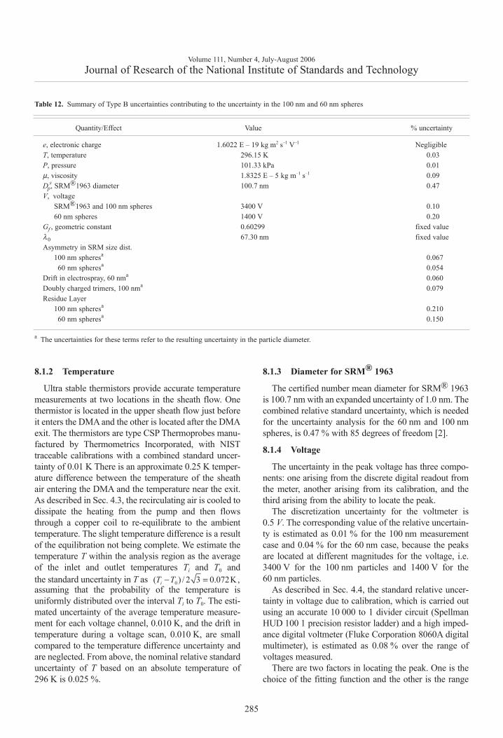
8.1.2 Temperature
Ultra stable thermistors provide accurate temperaturemeasurements at two locations in the sheath flow. Onethermistor is located in the upper sheath flow just beforeit enters the DMA and the other is located after the DMAexit. The thermistors are type CSP Thermoprobes manu-factured by Thermometrics Incorporated, with NISTtraceable calibrations with a combined standard uncer-tainty of 0.01 K There is an approximate 0.25 K temper-ature difference between the temperature of the sheathair entering the DMA and the temperature near the exit.As described in Sec. 4.3, the recirculating air is cooled todissipate the heating from the pump and then flowsthrough a copper coil to re-equilibrate to the ambienttemperature. The slight temperature difference is a resultof the equilibration not being complete. We estimate thetemperature T within the analysis region as the averageof the inlet and outlet temperatures Ti and T0 andthe standard uncertainty in T asassuming that the probability of the temperature isuniformly distributed over the interval Ti to T0. The esti-mated uncertainty of the average temperature measure-ment for each voltage channel, 0.010 K, and the drift intemperature during a voltage scan, 0.010 K, are smallcompared to the temperature difference uncertainty andare neglected. From above, the nominal relative standarduncertainty of T based on an absolute temperature of296 K is 0.025 %.
8.1.3 Diameter for SRM® 1963
The certified number mean diameter for SRM® 1963is 100.7 nm with an expanded uncertainty of 1.0 nm. Thecombined relative standard uncertainty, which is neededfor the uncertainty analysis for the 60 nm and 100 nmspheres, is 0.47 % with 85 degrees of freedom [2].
8.1.4 Voltage
The uncertainty in the peak voltage has three compo-nents: one arising from the discrete digital readout fromthe meter, another arising from its calibration, and thethird arising from the ability to locate the peak.
The discretization uncertainty for the voltmeter is0.5 V. The corresponding value of the relative uncertain-ty is estimated as 0.01 % for the 100 nm measurementcase and 0.04 % for the 60 nm case, because the peaksare located at different magnitudes for the voltage, i.e.3400 V for the 100 nm particles and 1400 V for the60 nm particles.
As described in Sec. 4.4, the standard relative uncer-tainty in voltage due to calibration, which is carried outusing an accurate 10 000 to 1 divider circuit (SpellmanHUD 100 1 precision resistor ladder) and a high imped-ance digital voltmeter (Fluke Corporation 8060A digitalmultimeter), is estimated as 0.08 % over the range ofvoltages measured.
There are two factors in locating the peak. One is thechoice of the fitting function and the other is the range
285
Volume 111, Number 4, July-August 2006Journal of Research of the National Institute of Standards and Technology
Table 12. Summary of Type B uncertainties contributing to the uncertainty in the 100 nm and 60 nm spheres
Quantity/Effect Value % uncertainty
e, electronic charge 1.6022 E – 19 kg m2 s–1 V–1 NegligibleT, temperature 296.15 K 0.03P, pressure 101.33 kPa 0.01µ, viscosity 1.8325 E – 5 kg m–1 s–1 0.09Dp
s, SRM®1963 diameter 100.7 nm 0.47V, voltage
SRM®1963 and 100 nm spheres 3400 V 0.1060 nm spheres 1400 V 0.20
Gf , geometric constant 0.60299 fixed valueλ0 67.30 nm fixed valueAsymmetry in SRM size dist.
100 nm spheresa 0.06760 nm spheresa 0.054
Drift in electrospray, 60 nma 0.060 Doubly charged trimers, 100 nma 0.079Residue Layer
100 nm spheresa 0.21060 nm spheresa 0.150
a The uncertainties for these terms refer to the resulting uncertainty in the particle diameter.
0( ) / 2 3 0.072K,iT T− =

over which the fit is made. The cubic function was usedto allow a skewness in the shape of the distribution nearthe peak, which is not included in a Gaussian fit. Overthe range of the fits, N/Np > 0.75, the Gaussian fit isessentially the same as a quadratic fit for finding thepeak voltage. To assess the sensitivity to the fittingfunction, selected data sets (five data sets for eachparticle size) were also fit with a quadratic function anda quartic function. The data were fit over the ranges ofabout N/Np > 0.75 and N/Np > 0.85 to assess the sensi-tivity of the results to the fitting range, which alsochanged the number of points in the fitting. For the100.7 nm SRM and for the new 100 nm standard, theaverage deviation of the quadratic and quartic fits rela-tive to the cubic were both about 1.8 V and the rangeeffect was also about 1.8 V. We estimated the combinedstandard uncertainty of these two components by theroot-sum-of-squares and obtained 2.5 V, which equals arelative uncertainty of 0.07 % of 3400 V. For the 60 nmspheres, the average deviation of the quadratic andquartic fits relative to the cubic were about 13 V and1 V and the range effect was 4.4 V for the quadraticcompared to about 1.8 V for the cubic. Both of the largedeviations observed for the quadratic fitting functionare a result of the skewness in the distribution, whichis not accounted for in the quadratic fit. Thus, theanomalous results for the quadratic fit are not relevant.Based on the range effect for the cubic (1.8 V) and theagreement between the cubic and quartic (1 V), weadopt the same estimate for the peak uncertainty, 2.5 V,as for the 100 nm spheres. Because of the lower nomi-nal voltage for the 60 nm spheres (1400 relative to3400), the relative uncertainty is increased to 0.18 %.The total voltage uncertainty is computed as the root-sum-of-squares of the three components with a resultof 0.10 % for the 100 nm spheres and 0.20 % for the60 nm spheres.
8.2 Propagation of Type B UncertaintiesThe goal of the Type B uncertainty analysis for the
60 nm diameter and 100 nm diameter particles is toexpress the relative uncertainty of the diameter in termsof the relative uncertainties in the measured voltages,temperature, and pressure, the diameter of SRM®1963; and the slip correction parameter A. The startingpoint is obtained from Eqs. (2) and (16),
(30)
where Dps is the certified diameter of SRM® 1963
(100.7 nm). The differential of the particle diameterdivided by itself can be expressed as:
(31)
We note that neither the viscosity nor the electroncharge differentials appear in this equation as theycancel out in the calibration measurement. If the cali-bration step was not conducted, then uncertainties inboth of these quantities would also appear.
The slip correction factor C can be expressed as afunction of the mean free path, particle diameter, andthe slip correction parameter A as follows:
(32)
As above, the differential of C divided by C is:
(33)
We note that the quantity A also has a small depend-ence on λ and Dp that is not included here, see [11] forthe extent of these quantities’ contribution. SubstitutingEq. (33) into Eq. (31), we obtain:
(34)
This equation is then solved for dDp/Dp,
(35)
The quantity λ is a function of pressure and temper-ature as indicated by Eq. (20). Recognizing that λ0 is afixed quantity without uncertainty, the differential ofthe mean free path can be expressed as:
(36)
The quantity S is the constant 110.4 K in Eq. (20).Substituting Eq. (36) into Eq. (35), we obtain the final
286
Volume 111, Number 4, July-August 2006Journal of Research of the National Institute of Standards and Technology
,sp p
s s
C VD DC V
=
.s
p ps ss
p s sp
dD dDdC dVdC dVD C C V VD
= − + + −
21 .p
C AD
λ= +
1 .p
p
dDdC C d dAC C A D
λλ
− = + −
2 1 11sp p s s s
sp s s sp
dD dD C dV CdV d CD C V V C CD
λλ
− −−= + − + −
11 1- .ps s
s s p
dDC dAC dA CC A C A C D
−− −+ −
( )( ) ( )
1
1 1
1sp ps s
sp sp
dD dDf C dVdVD f C f C V VD
= + −
( ) ( )( )
( )( )
( )( )
2 2 2 2
1 1 1
,s s s
s
f C f C f C f C dAd dAf C f C A f C A
λλ
−+ + −
( ) ( )1 22 1 1where and .C Cf C f C
C C− −= =
2 1 .d dPdTT T S P
λλ
= − − +

result in terms of the measured quantities and in termsof the uncertainties in the diameter of SRM® 1963 andthe uncertainty in the slip correction parameter,
(37)
Given that the variance of a sum of independent ran-dom variables is equal to the sum of the individual vari-ances, and then treating all terms in Eq. (37) except theterms involving A as independent random variables, wehave:
(38)
The terms A and As are dependent (correlated) and,thus, the associated variance, ur
2(Dp; A, As), includes acorrelation term in addition to the sum-of-squares ofthe individual terms:
(39)
In this expression, ur(A) is the relative standarduncertainty of A, ur(As) is the relative standard uncer-tainty of As, ur
Corr(A) is the correlated contribution to therelative uncertainty of A, and ur
Corr(As) is the correlatedcontribution to the relative uncertainty of As. To com-pute the quantity requires estimates for the total com-bined relative uncertainty in the slip correction para-
meter A and also estimates for the correlated contribu-tions to the uncertainty. We estimate the correlated con-tribution as the combined relative Type B uncertainty,considering this contribution to be potential bias thathas been introduced to the measurements. The Type Bcomponent used is computed by Kim et al. [12] and isbased on propagating the effect of the uncertainty ineach variable when computing the total uncertainty.The uncertainty in the calibration diameter is shown tobe the major contributor to the uncertainty in A. If thetrue diameter were some amount larger than the meas-ured diameter, then the value of A would be underesti-mated for all values of A. Our use of a calibration par-ticle introduces the correlation effect since the values ofA for both the unknown particle size (60 nm or 100 nm)and the SRM® 1963 would be shifted by almost thesame amount from an error in the calibration diameter.The other Type B components of the uncertainty arelikewise correlated. Values for the Type A and Type Buncertainties in the slip correction parameter A basedon Eq. (25) in Kim et al. [12] are provided in Table 13.The computed value of ur(Dp; A, As), based on Eq. (39)with the correlation effect is noted to be seven timessmaller for both the 100 nm spheres and the 60 nmspheres when compared to results obtained whenignoring correlation.
Next, we compute the relative Type B uncertaintybased on Eq. (38) making use of the results in Tables 12and 13. Table 14 presents each of the six termsexpressed as uncertainties, i.e., the square root of theindividual terms in Eq. (38). The combined uncertaintyobtained by propagating the individual uncertaintiesis found to be 0.494 % for the 100 nm spheres and0.469 % for the 60 nm spheres. The uncertainty of thediameter for the SRM® 1963 dominates the overalluncertainty with the next largest term being theslip correction factor term. It is important to notethat if the correlation effect had not been accounted for,the slip correction would have been the dominantuncertainty and the value of ur(Dp) would haveincreased by more than a factor of 1.8 to 0.92 %and 0.90 % for the 100 nm and 60 nm spheres,respectively.
8.3 Additional Uncertainty IssuesA number of other potential sources of uncertainty
were examined including the effects of slip correction,flow ratio, size distribution width for the 100 nmspheres, flow matching, drift in the number concen-tration measurement, multiply charged spheres, aresidue layer, and asymmetry in the size distributionof SRM® 1963.
287
Volume 111, Number 4, July-August 2006Journal of Research of the National Institute of Standards and Technology
( )( ) ( ) ( )
1
1 1 1
1 1sp ps s
sp sp
dD dDf C dVdVD f C f C V f C VD
= + −
( )( )
( )( )
( ) ( )( )
2 2 2 2
1 1 1
s ss
s
f C f C f C f CdAdAf C A f C A f C
−+ − + ×
( ) ( )( )
2 2
1
2 .sf C f CT dT dPT S T f C P
− − − +
( ) ( )( ) ( ) ( ) ( )
2 2
12
1 1
1s sr p r p r
f Cu D u D u V
f C f C
= +
( ) ( ) ( )2
2
1
1 ; ,r s r p su V u D A Af C
+ +
( ) ( )( ) ( )
2
2 2
1
2sr
f C f C T u Tf C T S
− + − +
( ) ( )( ) ( )
2
2 2
1
.sr
f C f Cu P
f C −
+
( ) ( )( ) ( ) ( )
( ) ( )2 2
2 22 2 2
1 1
; , sr s r r s
f C f Cu Dp A A u A u A
f C f C
= +
( )( )
( )( ) ( )( ) ( )( )2 2
1 1
2 .s Corr Corrr r
f C f Cu A u A
f C f C
−

8.3.1 Slip Correction
The DMA data were analyzed using both the Kimet al. [12] expression for the slip correction and theAllen and Raabe expression [11]. The slip correctionfactor is used twice. First the factor is used with the cal-ibration particles to determine the corrected flow.Secondly it is used with the concentration vs. voltagedistribution of the unknown particle size to determinethe peak particle size. For the 100 nm diameter particlesize, the choice of the slip correction changes theparticle size by about 0.02 nm—essentially no effect.This is because the size of the calibration particle is soclose to the 100 nm sphere. In the case of the 60 nmspheres, the mean particle size increases by 0.38 %from 60.45 nm to 60.68 nm. We have chosen to use theKim et al. expression [12] for the slip correctionbecause it includes a quantitative uncertainty treatment.Allen and Raabe’s analysis does not include a treatmentof the effect of the Type B uncertainties. The resultbased on the Allen and Raabe expression is presentedbecause this expression has been widely used.
8.3.2 Flow Ratio
Our analysis assumes that the ratio of the aerosolflow to sheath flow is 0.025. As discussed in Sec. 3.6,there is an estimated uncertainty of the ratio equal to+ 2 %/– 7 %. The data from test g of the 60 nm sphereson February 16, 2005, was reanalyzed for the flow ratio
reduced by 7 % and it was found that the particlesizechanged by 0.02 nm, which corresponded to achange of 0.03 %. This is a negligible effect.
8.3.3 Width and Asymmetry of SRM® 1963 SizeDistribution
Our analysis assumed that the standard deviation ofthe size distribution for SRM® 1963 was 2.0 nm. Asindicated in Fig. 5, the DMA data are more consistentwith a Gaussian size distribution with a standard devia-tion of 1.8 nm compared to 2.0 nm. In this case the effectof changing the width of the size distribution on thecorrected flow was assessed for run g on September 20,2004. The percentage change in the flow rate was– 0.01 %, which would produce a negligible change inthe diameter of the 100 nm spheres.
For the Gaussian distribution, the number meandiameter and the peak diameter are the same.Measurements of the SRM size distribution carried outwith the electrospray indicated a slight skewness in thedistribution towards smaller particle sizes. This willresult in the peak particle size being skewed to a largersize.
To determine the effect of this asymmetry on themeasured diameter, we modeled the SRM® 1963 sizedistribution as an asymmetric Gaussian with thefollowing form:
288
Volume 111, Number 4, July-August 2006Journal of Research of the National Institute of Standards and Technology
Table 13. Slip correction parameter Aa uncertainty for T = 296.15 K and P = 101.33 kPa
ur (Dp; A, As) ur (Dp; A, As)Dp, nm C ur
A(A) urB(A) ur With correlation Without correlation
100.70 2.8634 0.217 % 1.388 % 1.404 %101.60 2.8449 0.218 % 1.391 % 1.409 % 0.121 % 0.784 %60.46 4.2807 0.199 % 1.239 % 1.251 % 0.107 % 0.750 %
a The quantities urA(A), ur
B(A), and ur are the Type A uncertainty, the Type B uncertainty, and the combined uncertainty for the slip correctionparameter A. The quantity ur (Dp; A, As) is the uncertainty in the particle diameter arising from the uncertainties in the slip correction parameterfor the measured particle, A, and for the 100.7 nm SRM® 1963 particles, As .
Table 14. Combined relative Type B uncertainty and components for Eq. (38)
Term 1, Term 2, Term 3, Term 4, Term 5, Term 6,Dp, nm Dp for SRM V V for SRM A, As T P ur (Dp)
101.60 0.471 % 0.061 % 0.060 % 0.121 % 5.3 E – 5 % 1.4 E – 5 % 0.494 %60.46 0.439 % 0.113 % 0.057 % 0.107 % 0.009 % 6.5 E – 4 % 0.469 %
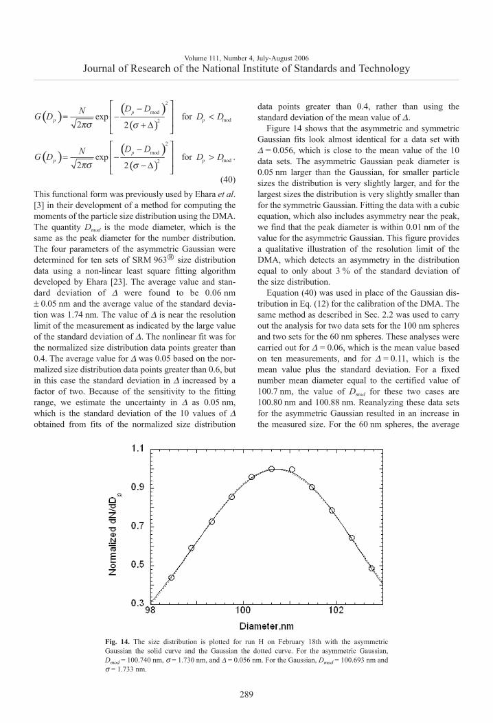
(40)This functional form was previously used by Ehara et al.[3] in their development of a method for computing themoments of the particle size distribution using the DMA.The quantity Dmod is the mode diameter, which is thesame as the peak diameter for the number distribution.The four parameters of the asymmetric Gaussian weredetermined for ten sets of SRM 963 size distributiondata using a non-linear least square fitting algorithmdeveloped by Ehara [23]. The average value and stan-dard deviation of ∆ were found to be 0.06 nm± 0.05 nm and the average value of the standard devia-tion was 1.74 nm. The value of ∆ is near the resolutionlimit of the measurement as indicated by the large valueof the standard deviation of ∆. The nonlinear fit was forthe normalized size distribution data points greater than0.4. The average value for ∆ was 0.05 based on the nor-malized size distribution data points greater than 0.6, butin this case the standard deviation in ∆ increased by afactor of two. Because of the sensitivity to the fittingrange, we estimate the uncertainty in ∆ as 0.05 nm,which is the standard deviation of the 10 values of ∆obtained from fits of the normalized size distribution
data points greater than 0.4, rather than using thestandard deviation of the mean value of ∆.
Figure 14 shows that the asymmetric and symmetricGaussian fits look almost identical for a data set with∆ = 0.056, which is close to the mean value of the 10data sets. The asymmetric Gaussian peak diameter is0.05 nm larger than the Gaussian, for smaller particlesizes the distribution is very slightly larger, and for thelargest sizes the distribution is very slightly smaller thanfor the symmetric Gaussian. Fitting the data with a cubicequation, which also includes asymmetry near the peak,we find that the peak diameter is within 0.01 nm of thevalue for the asymmetric Gaussian. This figure providesa qualitative illustration of the resolution limit of theDMA, which detects an asymmetry in the distributionequal to only about 3 % of the standard deviation ofthe size distribution.
Equation (40) was used in place of the Gaussian dis-tribution in Eq. (12) for the calibration of the DMA. Thesame method as described in Sec. 2.2 was used to carryout the analysis for two data sets for the 100 nm spheresand two sets for the 60 nm spheres. These analyses werecarried out for ∆ = 0.06, which is the mean value basedon ten measurements, and for ∆ = 0.11, which is themean value plus the standard deviation. For a fixednumber mean diameter equal to the certified value of100.7 nm, the value of Dmod for these two cases are100.80 nm and 100.88 nm. Reanalyzing these data setsfor the asymmetric Gaussian resulted in an increase inthe measured size. For the 60 nm spheres, the average
289
Volume 111, Number 4, July-August 2006Journal of Research of the National Institute of Standards and Technology
( ) ( )( )
2
modmod2exp for
2 2p
p p
D DNG D D Dπσ σ
− = − < + ∆
( ) ( )( )
2
modmod2exp for .
2 2p
p p
D DNG D D Dπσ σ
− = − > − ∆
Fig. 14. The size distribution is plotted for run H on February 18th with the asymmetricGaussian the solid curve and the Gaussian the dotted curve. For the asymmetric Gaussian,Dmod = 100.740 nm, σ = 1.730 nm, and ∆ = 0.056 nm. For the Gaussian, Dmod = 100.693 nm andσ = 1.733 nm.

increase in diameter was 0.042 nm for ∆ = 0.06 nm and0.075 nm for ∆ = 0.11 nm. For the 100 nm spheres, theaverage increase was 0.050 nm for ∆ = 0.06 nm and0.095 nm for ∆ = 0.11 nm. The number of significantfigures in the coefficients for the best fit equation wasincreased from 5 to 7 for one of the 100 nm data sets toobtain an accurate estimate of the change in the dia-meter. The results from the two data sets agreed withinabout 10 %. The values for ∆ = 0.06 nm are used inadjusting the value of the final diameters in Sec. 8.4. Theuncertainty in the correction, u(asym) is estimated as thedifference between the changes in the particle diametersfor ∆ = 0.11 nm and ∆ = 0.06 nm. The resulting valuesfor u(asym) are 0.033 nm for the 60 nm spheres and0.045 nm for the 100 nm spheres.
8.3.4 Brownian MotionIn our analysis of the transfer function Ω, the effect of
the Brownian motion is not included. As the particlesmove from the inlet to the outlet, the random Brownianmotion will cause the particle trajectory to be perturbed.The resulting transfer function has been solved in closedform [24], and an explicit expressions for the peak valueof the transfer function and its standard deviation havebeen obtained as a product of a diffusion dependentcorrection term multiplied by the expression without dif-fusion [25]. As seen in Table 15, the transfer function isbroadened by a factor of 1.09 for the 100 nm spheres andby 1.21 for the 60 nm spheres.
The effect of diffusion on the peak particle size wasassessed by first computing the concentration vs voltagedistribution using Eq. (12) and then computing the distri-bution again using a version of Eq. (12) with the transferfunction modified to include the effect of particle diffu-sion [23,24]. The size distribution G(Dp) was then com-puted using Eq. (14) and the peak in the size distributionobtained. The parameters for the two Gaussian size
distributions were number mean diameters of 101.60 nmand 60.70 nm and standard deviation of 2.6 nm and4.3 nm, respectively. In both cases, the differencebetween the peak diameter with diffusion and withoutdiffusion was negligible—less than 0.01 nm.
8.3.5 Mismatch of FlowThe estimated mismatch in the sheath flow versus
the excess flow is 0.01 % of the sheath flow. This slightmismatch means that the aerosol flow in, Qa, will beslightly different than the aerosol flow out, Qs. This willresult in a transfer function with a trapezoidal shaperather than a triangular shape. The height of the trape-zoid is equal to Qs / Qa in the case that Qs > Qa. For theabove example, the peak in the transfer function isslightly reduced from 1.000 to 0.996. This is less of aneffect than for Brownian motion where the peaks in thetransfer function given in Table 15 are 0.78 (60 nmspheres) and 0.86 (100 nm spheres). Clearly, the flowmismatch effect is negligible.
8.3.6 Drift in the Number ConcentrationThere are two sources of uncertainty in the number
concentration measurement by the CPC (condensationparticle counter). One is a random uncertainty and thesecond arises from a drift in the generator output. Therandom variability arises from the Poisson countingstatistics for the aerosol flowing into the CPC. Theuncertainty is equal to one divided by the square root ofthe number of particles counted over a 20 s averagingperiod for the measurement. For the lowest concentra-tion measured, 125 part./cm–3, and a CPC flow rate of5 cm3/s, the number of particles counted is 12,500, andthe uncertainty is 0.89 %. The effect of this uncertaintyis included in the Type A uncertainty determined fromthe repeat measurements of the peak particle size forthe 60 nm spheres and the 100 nm spheres.
290
Volume 111, Number 4, July-August 2006Journal of Research of the National Institute of Standards and Technology
Table 15. Effect of particle diffusion on the peak height and dimensionless width of the transfer function
Dp, nm Diff, m2/s ΩDiff (peak) / ΩNoDiff (peak)a σDiff / σNoDiffb
10 5.52 E-08 0.25 3.9930 6.41 E-09 0.59 1.6560.7 1.68 E-09 0.78 1.21
101.6 6.62 E-10 0.86 1.09
a Correction factor to peak value of the transfer fraction, which occurs at x = 1, resulting from particle diffusion.b Correction factor for the width of the transfer function resulting from diffusion.
The drift in the number concentration of the 100 nmspheres using the pneumatic nebulizer is on averageabout 1 % and at most 2 % over the measurementinterval of about 12 minutes. This drift has a negligibleeffect on the measured particle size. The drift in thenumber concentration of the 60 nm spheres and 100 nmspheres produced with the electrospray was larger withvalues up to 11 %. Measurements were made at a volt-age close to the peak voltage at the start of the experi-ment, at the middle, and at the end to estimate a lineardrift in the concentration over the course of the experi-ment for the experiments carried out with the electro-spray. All the number concentration data were adjustedwith the linear fit to give the estimated concentration atthe time of the peak measurement. These adjustmentswere made for both the SRM calibration measurementused to find the corrected flow and for the 60 nm spheremeasurements. The effect of the drift on the SRM cali-bration was a factor of about 3 smaller than for the 60 nmspheres because of the much narrower size distribution.The largest adjustment to the peak particle size was0.189 nm and the average value of the absolute magni-tude of the changes was 0.072 nm with a standard devi-ation of 0.063 nm. Seven adjustments resulted in anincrease in the diameter, five a decrease, and the averagediameter increased by 0.01 nm. We do not know thecause of the drift. It may be fortuitous that we observedabout an equal number of plus and minus drifts. Thelinear drift correction is useful correction; however,more complex time variations were observed. Whilemonitoring the concentration at a fixed voltage over aperiod of about 30 minutes, we observed a drift with twoslopes in one case and a dip in concentration followed bya return to the original concentration in a second case.There is an uncertainty in the drift correction fromsuch effects and we estimate this drift uncertainty as0.036 nm, which is 1/2 the average of the absolutemagnitudes of the changes. The corresponding relativeuncertainty, ur(drift), is equal to 0.060 % for the meas-urement of the 60 nm spheres.
8.3.7 Multiply Charged SpheresIn Sec. 6.1 it was pointed out that mobility of doublet
trimers would overlap the mobility peak of the singletmonomers for the 100 nm spheres. A doublet trimerwould appear at half the voltage of the same singlettrimer. The number concentration of singlet trimers inthis overlapping region was found to be about one-tenththe concentration of the singlet monomers (run b,October 14, 2004, Fig. 8). The ratio of charging proba-bilities of a doublet trimer to a singlet monomer was
estimated using Wiedensohler’s expression [16] and thesurface area equivalent sphere for the trimer. Using thisinformation, the number concentration of such doublettrimers for run b, September 20, 2004 (Fig. 4) was esti-mated and this number was subtracted for the total num-ber concentration data for each voltage. The correctionwas about 1 % at the lower end of the size distributionand increased to almost 3 % at the upper end. The sizedistribution G(Dp) was obtained from the net concentra-tion data and the peak diameter was determined. Theresulting diameter was 101.62 nm compared to the un-corrected value of 101.70 nm. This effect of 0.079 % isused as an estimate of ur(doublet), the Type B relativestandard uncertainty resulting from the doublet trimer.
The effect of multiplet multimers is at least two ordersof magnitude lower for the 60 nm spheres because of themuch lower fraction of multimers produced, less than1 %, when using the electrospray generator.
8.3.8 Residue Layer from Impurities in PSLSuspension
The polystyrene spheres measured as an aerosolinclude a residue layer. This results from the evaporationof the droplet containing the polystyrene sphere. Thenonvolatile contaminants from the dilution water andfrom the electrolyte and soluble fraction of the surfactantin polystyrene sphere suspension leave a residue layerover the sphere as the water evaporates. This will resultin the sphere size as an aerosol being slightly larger thanthe diameter of the polystyrene sphere. Two methods forestimating the residue layer thickness are presented andthe impact of this layer on the measured sphere size andon the uncertainty are presented.
8.3.8.1 Direct Measurement of ResidueThe measurement of the size distribution of the
residue particles resulting from the evaporation ofdroplets not containing spheres provides a direct meas-urement of the residue thickness. It is assumed that thedroplet distribution leading to the residue particles is thesame as that for the droplets containing the spheres. Thevolume of the aerosol particles is the sum of the volumeof the polystyrene sphere and the residue particle:
(41)
where Da is the diameter of the aerosol particle, Dps isthe diameter of the polystyrene sphere, and Dr is thediameter of the residue particle. Solving for Dps in thelimit (Dr / Da)1/3 << 1, one obtains:
291
Volume 111, Number 4, July-August 2006Journal of Research of the National Institute of Standards and Technology
( )3 3 31 1 ,6 6a ps rD D Dπ π= +
(42)
The size distributions of the residue particles aremeasured using the DMA. The conditions are identicalto those used for the particle size distribution in terms ofthe solution concentrations and the operation conditionsfor the pneumatic generator. The conditions for the elec-trospray in terms of voltage were close but not identicalto those used previously. The slight difference arosefrom optimizing the stability of the generator. In all casesthe generator was operated in the pulsating mode withthe current within 10 % of the value used during thecertification measurements.
For the electrospray, there are less than 0.05 cm–3
residue particles counted by the condensation particlecounter (CPC) for particle sizes less than 50 nm for thebuffer and for SRM® 1963. The buffer solution containsammonium acetate, which has a high vapor pressure andsublimes as an aerosol. This value is close to the mini-mum count rate for the condensation particle counter andabout four orders of magnitude smaller than the peakparticle concentrations for the SRM, (200 – 400) cm–3.The minimum particle size detected by the DMA/CPCcombination for the flow settings used is about 12 nm.The residue particles are smaller than this size. An upperbound for the difference between Da and Dps is deter-mined to be 0.06 nm from Eq. (42) assuming Dr equal to12 nm and Da = 100.7 nm.
The size distribution of the residue particles producedvia the electrospray is similar for the 60 nm spheres, forSRM® 1963, and for the buffer solution for particlessizes less than 25 nm as indicated in Fig. 15. The logarith-mic size distribution, dN/dlnDr, is used because size dis-tribution of sprayed liquids are typically better approxi-mated by lognormal distribution than by a normal distri-bution. The upper bound of the residue size is againestimated as 12 nm. This results in an upper bound for thedifference between Dps and Da equal to 0.16 nm assumingDa = 60.5 nm.
At a diameter of 27 nm, the size distribution for the60 nm residue particles increases to a value of about0.5 cm–3 (See Fig. 15) compared to a value of about0.02 cm–3 for SRM® 1963 and the buffer. The distributioncontinues to increase rapidly with increasing particlediameter, while the distribution for the SRM® 1963 andbuffer solution remain flat. The rapid increase for the60 nm case is a result of the long tail in the 60 nm sizedistribution as indicated in Figs. 12 and 13.
For the pneumatic nebulizer, the apparent peak dia-meter is within a few percent of 21 nm for the dilutionwater, for the SRM® 1963, and for the 100 nm spheres as
shown in Fig 16. The actual peak in the distribution is sig-nificantly smaller than 21 nm. The reason for the overesti-mate of the peak is that small residue particles generatedby PSL suspensions are lost to the walls in the DMAor notcounted by the CPC. In Fig. 17, the size distribution isplotted for the residue particles produced by nebulizing a0.1 % mass fraction sucrose solution. In both the PSLsphere case and the sucrose cases, the number of dropletsproduced are expected to be similar and likewise the num-ber of residue particles. However, the total number con-centration of the residue particles produced is about 25times smaller for the PSL suspension compared with the0.1 % mass fraction sucrose suspension. It is inferred thatmost of the reduction is from the losses of small particles.If the residue particle size distribution for the PSL suspen-sion is similar in shape to the distribution for the sucrosesolution, the peak particle size would be at least a factortwo smaller than the apparent size of 21 nm.
The probability of a droplet containing a PSL sphere isexpected to be proportional to the product of the size dis-tribution function dN/dlnDp multiplied times thevolume of the droplet which is equal to the volumedistribution, dV/dlnDp. The larger the droplet the morelikely there is a polystyrene sphere in the droplet. Thispeak droplet size, Dp(droplet), will produce a residueparticle size, Dp(residue), equal to the peak in the residuevolume distribution. For the size distributions shown inFig. 16, this size is about 25 nm. As discussed above, theactual peak in the residue size distribution is likely at leasta factor of two smaller size resulting in a correspondingsmaller value of Dp(residue). A value of Dp(residue) equalto 20 nm is an upper bound estimate. From Eq. (42) wefind for the SRM® 1963 spheres and for the 100 nmspheres, that the difference between Da and Dps in bothcases is 0.26 nm.
The previous analysis assumes that the probability of aPSL sphere being in a droplet is proportional to thevolume of the droplet. This is a reasonable approximationif the droplet volume V(droplet) is much smaller than theaverage volume of the liquid per particle V(liq). If V(liq)is equal to V(droplet), this condition would break downwith almost every droplet containing a particle. Theresidue particles would probably be dominated by thesmall size range of the droplet distribution. To estimateV(liq), the number concentration of spheres per volume ofthe liquid nebulized is calculated. The number concentra-tions nt of the 60.46 nm spheres and the 101.6 nm spheresin the vials with a nominal volume fraction of 0.005 arecomputed to be (4.3 × 10¹³ and 9.1 × 10¹²) cm–3 using thefollowing equation:
(43)
Volume 111, Number 4, July-August 2006Journal of Research of the National Institute of Standards and Technology
292
311 .3
rps a
a
DD DD
= −
( )3
6(0.005) .t
p
nDπ
=
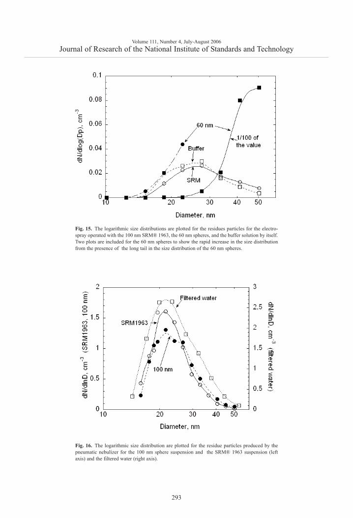
Volume 111, Number 4, July-August 2006Journal of Research of the National Institute of Standards and Technology
293
Fig. 15. The logarithmic size distributions are plotted for the residues particles for the electro-spray operated with the 100 nm SRM® 1963, the 60 nm spheres, and the buffer solution by itself.Two plots are included for the 60 nm spheres to show the rapid increase in the size distributionfrom the presence of the long tail in the size distribution of the 60 nm spheres.
Fig. 16. The logarithmic size distribution are plotted for the residue particles produced by thepneumatic nebulizer for the 100 nm sphere suspension and the SRM® 1963 suspension (leftaxis) and the filtered water (right axis).
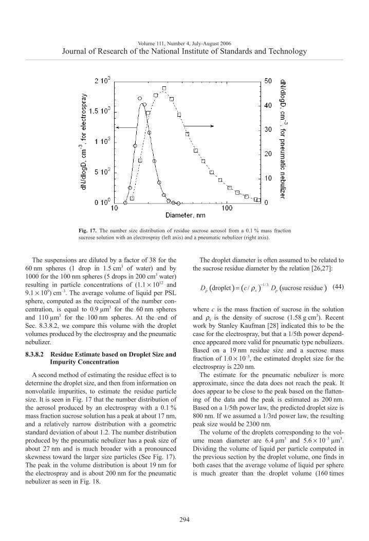
The suspensions are diluted by a factor of 38 for the60 nm spheres (1 drop in 1.5 cm3 of water) and by1000 for the 100 nm spheres (5 drops in 200 cm3 water)resulting in particle concentrations of (1.1 × 10¹² and9.1 × 109) cm–3. The average volume of liquid per PSLsphere, computed as the reciprocal of the number con-centration, is equal to 0.9 µm3 for the 60 nm spheresand 110 µm3 for the 100 nm spheres. At the end ofSec. 8.3.8.2, we compare this volume with the dropletvolumes produced by the electrospray and the pneumaticnebulizer.
8.3.8.2 Residue Estimate based on Droplet Size andImpurity Concentration
A second method of estimating the residue effect is todetermine the droplet size, and then from information onnonvolatile impurities, to estimate the residue particlesize. It is seen in Fig. 17 that the number distribution ofthe aerosol produced by an electrospray with a 0.1 %mass fraction sucrose solution has a peak at about 17 nm,and a relatively narrow distribution with a geometricstandard deviation of about 1.2. The number distributionproduced by the pneumatic nebulizer has a peak size ofabout 27 nm and is much broader with a pronouncedskewness toward the larger size particles (See Fig. 17).The peak in the volume distribution is about 19 nm forthe electrospray and is about 200 nm for the pneumaticnebulizer as seen in Fig. 18.
The droplet diameter is often assumed to be related tothe sucrose residue diameter by the relation [26,27]:
(44)
where c is the mass fraction of sucrose in the solutionand ρs is the density of sucrose (1.58 g cm3). Recentwork by Stanley Kaufman [28] indicated this to be thecase for the electrospray, but that a 1/5th power depend-ence appeared more valid for pneumatic type nebulizers.Based on a 19 nm residue size and a sucrose massfraction of 1.0 × 10⁻³, the estimated droplet size for theelectrospray is 220 nm.
The estimate for the pneumatic nebulizer is moreapproximate, since the data does not reach the peak. Itdoes appear to be close to the peak based on the flatten-ing of the data and the peak is estimated as 200 nm.Based on a 1/5th power law, the predicted droplet size is800 nm. If we assumed a 1/3rd power law, the resultingpeak size would be 2300 nm.
The volume of the droplets corresponding to the vol-ume mean diameter are 6.4 µm3 and 5.6 × 10⁻³ µm3.Dividing the volume of liquid per particle computed inthe previous section by the droplet volume, one finds inboth cases that the average volume of liquid per sphereis much greater than the droplet volume (160 times
Volume 111, Number 4, July-August 2006Journal of Research of the National Institute of Standards and Technology
294
Fig. 17. The number size distribution of residue sucrose aerosol from a 0.1 % mass fractionsucrose solution with an electrospray (left axis) and a pneumatic nebulizer (right axis).
( ) ( ) ( )1/ 3droplet / sucrose residuep s pD c Dρ −=

larger for the 60 nm sphere and 17 times larger for the100 nm spheres). Thus the assumption that the probabil-ity of a particle being in a sphere is proportional to thedroplet volume is reasonable.
To estimate the residue size from the droplet, we needan estimate of the non-volatile impurities in the PSLsuspension. For the 100 nm spheres, the mass fraction ofthe non-volatile material included 2.1 × 10⁻⁴ surfactantand 6.0 × 10⁻⁵ electrolyte remaining after the synthesis.Assuming half of the surfactant on the particle surface,the total mass fraction of non-volatile material in theliquid is 1.7 × 10⁻⁴. The mass, mi, of the non-volatileimpurities in the five droplets added to 200 ml of filtereddeionized water is estimated based on an estimateddroplet size of 0.040 cm3:
(45)
The mass fraction of these nonvolatile impurities in the200 ml of water is 1.7 × 10⁻⁷. To obtain the total mass frac-tion of non-volatile impurities one must add the approxi-mately 1 × 10⁻⁶ mass fraction [27] resulting from theimpurities in the filtered-deionized water. Assuming adensity of the impurities deposited on the sphere afterevaporation of the water of 1.5 g/cm3, the resultingvolume fraction of non-volatile impurities, Vr is 7.8 × 10⁻⁷.
The increase in the PSL sphere diameter ∆Dp resultingfrom the impurity can be estimated based on the volumefraction of the impurities and the diameters of the dropletfrom the pneumatic atomizer (2000 nm) and the PSLsphere (101.6 nm) using the following formula[27]:
(46)
This value of 0.30 nm is close to the estimate of 0.26based on the residue particle size.
For the SRM® 1963, there was no surfactant added tothe suspension. In this case the estimated value of Vr isabout 7.1 × 10⁻⁷ and the estimated thickness is reducedslightly to a value of about 0.27 nm.
For the 60 nm spheres, there is no surfactant addedand there is no information regarding other non-volatileimpurities. We estimate the mass fraction of the impuri-ties in the droplet to be 6.0 × 10⁻⁵, which is equal to themass fraction of electrolyte impurities in the 101.6 nmspheres. In this case there is one drop of PSL spheres in1.5 cm3 of filtered-deionized water. Including the impu-rities in the dilution water, 1 × 10⁻⁶, the mass fraction ofthe diluted solution is 2.6 × 10⁻⁶ and Vr is 1.7 × 10⁻⁶
assuming a density of 1.5 g/cm3. From the formula
Volume 111, Number 4, July-August 2006Journal of Research of the National Institute of Standards and Technology
295
Fig. 18. The volume size distribution of residue sucrose aerosol from a 0.1 % mass fractionsucrose solution with an electrospray and a pneumatic nebulizer.
4 55(0.040)(1.7 10 ) 3.4 10 g .im − −= × = ×
( )3
2 0.30 nm .3
rp
ps
V D dropletD
D∆ = =

above, we find ∆Dp = 0.002 nm. This is more than anorder of magnitude smaller than the upper bound esti-mate of 0.12 nm based on the residue particle size. Theresidue diameter corresponding to a 220 nm dropletproduced by the electrospray and a volume fraction of1.7 × 10–6 would be 3.0 nm, which is well below thesmallest size measurable by the DMA used in this study.Thus it is not surprising that the value of ∆Dp estimatedfrom the residue size is a gross over estimate. Realizingthat there is a large uncertainty in the contaminant con-centration, a more realistic upper bound estimate of ∆Dp
is 0.01 nm for the 60 nm spheres, which corresponds toa contaminant volume fraction Vr = 8.5 × 10⁻⁶. FromEq. (46), the value of ∆Dp for the SRM® 1963 aerosolproduced by the electrospray is 0.003 nm assuming thesame contaminant concentration as the 60 nm spheres.
8.3.8.3 The Impact of the Residue Layer on theMeasured Peak Particle Sizesand Uncertainties
The estimated value of ∆Dp from the residue for the100.7 nm SRM® 1963 varies for the following threecases: the original measurement of SRM® 1963, themeasurement using the pneumatic atomizer, and themeasurement involving the electrospray. In the originalmeasurements of SRM® 1963 [2] an impactor was usedafter the nebulizer to remove the larger droplets. Theestimated residue increase to the diameter [27] was0.15 nm and the uncertainty range from the residueeffect on diameter is given as 0 % / 0.3 % of the meandiameter. An alternative statement of this result adoptedhere is that ∆Dp(orig) = 0.15 nm ± 0.15 nm. For thecurrent measurements with SRM® 1963 using thenebulizer, the estimated value of ∆Dp(Neb) = 0.26 nm,and for the measurements with the electrospray,∆Dp(ES) = 0.003 nm. The uncertainties in these estimatesare large. We assume that the uncertainty for the nebulizercase is the same as for the original study, ± 0.15 nm, andthat for the electrospray it is equal to the value of ∆Dp,± 0.003 nm.
The three different values of ∆Dp mean that the size ofthe SRM® 1963 as an aerosol is different in each of thethree measurements. For the original measurement [2],the peak aerosol size, Da
orig (peak), for SRM® 1963 is100.7 nm. For the other two cases, the peak aerosol sizeand the uncertainty associated with the residue measure-ment, u(residue), are given by:
(47)
(48)
where i = 1 corresponds to the pneumatic atomizer andi = 2 to the electrospray. The following values for thepeak diameter and uncertainty resulting from the residuelayer are given by: (100.81 ± 0.21) nm for the pneumat-ic nebulizer and (100.55 ± 0.15) nm for the electrospray.
The change in the size of the calibration particle willin turn cause a change in the diameter of the 100 nmspheres and the 60 nm spheres. To compute this change,the predicted number concentration of the aerosol exitingthe DMA is computed as a function of voltage usingEq.(5) based on the revised size of 100.55 for the SRM®1963 particles for the 60 nm spheres and 100.81 for the100 nm spheres. The peak voltage is computed and thecorrected flow determined as discussed in Sec. 2.2. Theresulting change in the mobility is computed usingEq.(15) and then the change in diameter is computedfrom the mobility using Eq.(2). The computed changefor the 60 nm spheres diameter is – 0.114 nm and for the100 nm sphere diameter is 0.110 nm. The computeduncertainties in the diameters resulting from the residuelayer uncertainty for the SRM are ± 0.114 nm for the60 nm spheres and ± 0.206 nm for the 100 nm spheres.
8.4 Bias Correction, Total Type B Uncertainty, andExpanded Uncertainty
Slight corrections are made to the sizes of the 100 nmand 60 nm spheres as a result of bias effects from theasymmetry in the size distribution of the SRM® 1963spheres, β(asym), and from the effect of the residue layeron the SRM® 1963 spheres, β(residue). The correcteddiameter, Dp(corr), is computed based on the followingsum:
(49)
The resulting values for Dp (corr) for the 100 nm spheresand the 60 nm spheres are 101.76 nm and 60.39 nm(Table 16).
The total relative type B uncertainty,the 60 nm spheres is estimated as the root-sum-of-squares of ur(Dp), ur(asym), ur(drift), and ur(residue), allgiven in Table 17. The resulting value of0.497 %. For the 100 nm spheres, estimated
Volume 111, Number 4, July-August 2006Journal of Research of the National Institute of Standards and Technology
296
( ) ( )i orig i origa a p pD peak D peak D D= + ∆ − ∆
( )( ) ( )2
2 2iai i
pip
D peaku residue D
D ∂
= ∆ ∂∆
( )2
2 ,ia orig
porigp
D peakD
D ∂
+ ∆ ∂∆
( ) ( ) ( ) ( ) .p pD corr D peak asym residueβ β= + +
TotalType B , forru
TotalType B isruType B isru
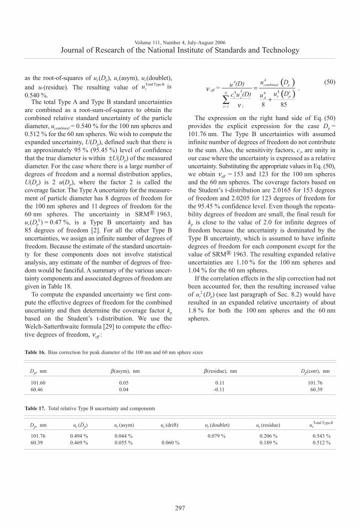
as the root-of-squares of ur(Dp), ur(asym), ur(doublet),and ur(residue). The resulting value of0.540 %.
The total Type A and Type B standard uncertaintiesare combined as a root-sum-of-squares to obtain thecombined relative standard uncertainty of the particlediameter, ucombined = 0.540 % for the 100 nm spheres and0.512 % for the 60 nm spheres. We wish to compute theexpanded uncertainty, U(Dp), defined such that there isan approximately 95 % (95.45 %) level of confidencethat the true diameter is within ±U(Dp) of the measureddiameter. For the case where there is a large number ofdegrees of freedom and a normal distribution applies, U(Dp) is 2 u(Dp), where the factor 2 is called thecoverage factor. The Type A uncertainty for the measure-ment of particle diameter has 8 degrees of freedom forthe 100 nm spheres and 11 degrees of freedom for the60 nm spheres. The uncertainty in SRM® 1963,ur(Dp
S) = 0.47 %, is a Type B uncertainty and has 85 degrees of freedom [2]. For all the other Type Buncertainties, we assign an infinite number of degrees offreedom. Because the estimate of the standard uncertain-ty for these components does not involve statisticalanalysis, any estimate of the number of degrees of free-dom would be fanciful. A summary of the various uncer-tainty components and associated degrees of freedom aregiven in Table 18.
To compute the expanded uncertainty we first com-pute the effective degrees of freedom for the combineduncertainty and then determine the coverage factor kp
based on the Student’s t-distribution. We use theWelch-Satterthwaite formula [29] to compute the effec-tive degrees of freedom, νeff :
(50)
The expression on the right hand side of Eq. (50)provides the explicit expression for the case Dp =101.76 nm. The Type B uncertainties with assumedinfinite number of degrees of freedom do not contributeto the sum. Also, the sensitivity factors, ci, are unity inour case where the uncertainty is expressed as a relativeuncertainty. Substituting the appropriate values in Eq. (50),we obtain νeff = 153 and 123 for the 100 nm spheresand the 60 nm spheres. The coverage factors based onthe Student’s t-distribution are 2.0165 for 153 degreesof freedom and 2.0205 for 123 degrees of freedom forthe 95.45 % confidence level. Even though the repeata-bility degrees of freedom are small, the final result forkp is close to the value of 2.0 for infinite degrees offreedom because the uncertainty is dominated by theType B uncertainty, which is assumed to have infinitedegrees of freedom for each component except for thevalue of SRM® 1963. The resulting expanded relativeuncertainties are 1.10 % for the 100 nm spheres and1.04 % for the 60 nm spheres.
If the correlation effects in the slip correction had notbeen accounted for, then the resulting increased valueof ur
2 (Dp) (see last paragraph of Sec. 8.2) would haveresulted in an expanded relative uncertainty of about1.8 % for both the 100 nm spheres and the 60 nmspheres.
Volume 111, Number 4, July-August 2006Journal of Research of the National Institute of Standards and Technology
297
TotalType B isru
Table 16. Bias correction for peak diameter of the 100 nm and 60 nm sphere sizes
Dp, nm β(asym), nm β(residue), nm Dp(corr), nm
101.60 0.05 0.11 101.7660.46 0.04 –0.11 60.39
Table 17. Total relative Type B uncertainty and components
Dp, nm ur (D–p) ur (asym) ur (drift) ur (doublet) ur (residue) urTotalTypeB
101.76 0.494 % 0.044 % 0.079 % 0.206 % 0.543 %60.39 0.469 % 0.055 % 0.060 % 0.189 % 0.512 %
( )( )
4
44 4.
8 85
4combined p
eff 4 sNr pi i A
ii=1
u D(D)u = u D(D)c u u
ν
ν
=
+∑
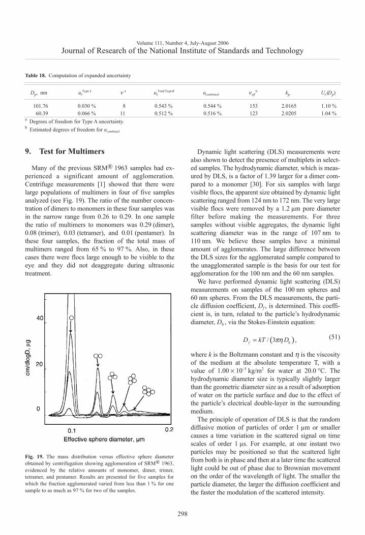
9. Test for Multimers
Many of the previous SRM® 1963 samples had ex-perienced a significant amount of agglomeration.Centrifuge measurements [1] showed that there werelarge populations of multimers in four of five samplesanalyzed (see Fig. 19). The ratio of the number concen-tration of dimers to monomers in these four samples wasin the narrow range from 0.26 to 0.29. In one samplethe ratio of multimers to monomers was 0.29 (dimer),0.08 (trimer), 0.03 (tetramer), and 0.01 (pentamer). Inthese four samples, the fraction of the total mass ofmultimers ranged from 65 % to 97 %. Also, in thesecases there were flocs large enough to be visible to theeye and they did not deaggregate during ultrasonictreatment.
Dynamic light scattering (DLS) measurements werealso shown to detect the presence of multiplets in select-ed samples. The hydrodynamic diameter, which is meas-ured by DLS, is a factor of 1.39 larger for a dimer com-pared to a monomer [30]. For six samples with largevisible flocs, the apparent size obtained by dynamic lightscattering ranged from 124 nm to 172 nm. The very largevisible flocs were removed by a 1.2 µm pore diameterfilter before making the measurements. For threesamples without visible aggregates, the dynamic lightscattering diameter was in the range of 107 nm to110 nm. We believe these samples have a minimalamount of agglomerates. The large difference betweenthe DLS sizes for the agglomerated sample compared tothe unagglomerated sample is the basis for our test foragglomeration for the 100 nm and the 60 nm samples.
We have performed dynamic light scattering (DLS)measurements on samples of the 100 nm spheres and60 nm spheres. From the DLS measurements, the parti-cle diffusion coefficient, Df , is determined. This coeffi-cient is, in turn, related to the particle’s hydrodynamicdiameter, Dh , via the Stokes-Einstein equation:
(51)
where k is the Boltzmann constant and η is the viscosityof the medium at the absolute temperature T, with avalue of 1.00 × 10⁻⁵ kg/m2 for water at 20.0 °C. Thehydrodynamic diameter size is typically slightly largerthan the geometric diameter size as a result of adsorptionof water on the particle surface and due to the effect ofthe particle’s electrical double-layer in the surroundingmedium.
The principle of operation of DLS is that the randomdiffusive motion of particles of order 1 µm or smallercauses a time variation in the scattered signal on timescales of order 1 µs. For example, at one instant twoparticles may be positioned so that the scattered lightfrom both is in phase and then at a later time the scatteredlight could be out of phase due to Brownian movementon the order of the wavelength of light. The smaller theparticle diameter, the larger the diffusion coefficient andthe faster the modulation of the scattered intensity.
Volume 111, Number 4, July-August 2006Journal of Research of the National Institute of Standards and Technology
298
Table 18. Computation of expanded uncertainty
Dp, nm urTypeA ν a ur
TotalTypeB ucombined νeffb kp Ur(Dp)
101.76 0.030 % 8 0.543 % 0.544 % 153 2.0165 1.10 %60.39 0.066 % 11 0.512 % 0.516 % 123 2.0205 1.04 %
a Degrees of freedom for Type A uncertainty.b Estimated degrees of freedom for ucombined
Fig. 19. The mass distribution versus effective sphere diameterobtained by centrifugation showing agglomeration of SRM® 1963,evidenced by the relative amounts of monomer, dimer, trimer,tetramer, and pentamer. Results are presented for five samples forwhich the fraction agglomerated varied from less than 1 % for onesample to as much as 97 % for two of the samples.
( )/ 3 ,f hD kT Dπη=

To process this rapidly changing light scatteringsignal, a photon correlator is used where each channelcounts photons arriving over a particular time span. Theintensity autocorrelation function is obtained by multi-plying the photon count at time t by the count at timet + τ, where τ is the delay time. For delay times overwhich the particles move only a small fraction of thewavelength of light (time on the order of 100 ns), thedegree of correlation is high. At long times, when thereis no correlation, the product of the two intensitiesapproaches the square of the time-averaged scatteringintensity. Generally, the autocorrelation function isnormalized to this long-time product.
For a monodisperse distribution of independentscatterers, the normalized intensity autocorrelation func-tion, G(τ), is an exponential function dependent on thediffusion coefficient Df and the wave vector magnitude q:
(52)
and where B is the baseline (long-time value of G(τ)), C1
is an instrumental coherence factor, λ is the wavelengthof light, θ is the scattering angle, and n0 the refractiveindex of the liquid. In our case the wavelength of light is633 nm (HeNe laser), the refractive index of water is1.33, and the scattering angle 90°.
For polydisperse size distributions, the autocorrelationfunction is expressed as an average over the distributionof particle masses where f (mp)dmp is equal to thenumber fraction of particles with mass between mp andmp + dmp.
(53)
where the factor mp2 accounts for light scattering intensity
being proportional to the square of the particle volume.A widely used method for analyzing the data is to expandln G(τ) of the autocorrelation function in a Taylor seriesabout τ = 0 resulting in the expression [31,32]:
(54)
The quantities DfZ , the z-average [31] diffusion coeffi-cient, and δDf Z, the variance of the z-average diffusioncoefficient, are defined below:
(55)
(56)
Since the diffusion coefficient is inversely proportion-al to the hydrodynamic diameter, Dh, the moments canbe expressed in terms of Dh. Equation (55), for example,becomes
(57)
Our measurements were carried out with a MalvernZetasizer 3000HS. The samples consisted of one or twodrops of the PSL samples diluted in 60 cm3 or 80 cm3 offiltered, deionized water. The samples were ultrasonicat-ed for about 10 s and then filtered with a 1.2 µm poresize filter before transfer to the sample cell. Filteringremoved large flocs and miscellaneous dust particles.The transfer was performed in a laminar-flow clean-airhood. Typically each measurement was carried out for60 s, and six repeat measurements were made for eachsample.
For the 60 nm spheres, three different samples wererun each day, and a sample of the 100 nm SRM® 1963was run at the beginning and end of the measurementsequence. The 100 nm sample was selected based onscreening 10 SRM® 1963 samples to find the one withthe smallest peak size. The major findings were littlesample-to-sample variability for ⟨Dh⟩Ζ
(see Table 19)for each sample (range from 59.3 nm to 63.4 nm) andan average of the six values of ⟨Dh⟩Ζ
, ⟨D– h⟩Ζ, equal to
60.5 nm ± 1.5 nm compared to 60.39 nm measured bythe DMA. This indicates at most a couple percent ofdimers, trimers, or larger multimers. The hydrodynamicdiameter of a dimer by DLS is 84 nm, a factor of 1.39times larger than a monomer [2]. Also, there is no indi-cation of a much larger presence of dimers in one bottlecompared to another. This data is important for futurecomparisons to assess whether agglomeration is takingplace in the samples over a period of time, as was thecase with SRM® 1963.
For the 100 nm spheres, three samples were measured,and for two of the samples, the measurements were madeat two different concentrations (See Table 20). For thisinstrument, the optimum concentration results in a pho-ton count rate in the range of (50,000 to 200,000)s–1.We observed little change in ⟨Dh⟩Ζ over the range(40,000 to 600,000)s–1. The value of ⟨D– h⟩Ζ is 99.8 nmcompared to the DMA size of 101.6 nm. There is no evidence of formation of dimers or trimers based onthis result.
Volume 111, Number 4, July-August 2006Journal of Research of the National Institute of Standards and Technology
299
( ) ( )21 exp 2 ,fG B C D qτ τ= + −
( )04 with sin / 2 ,
nq π θλ
=
( ) ( ) ( )( )2 2exp 2 ,p p f p pG B f m m q D m dmτ σ τ= + −∫
( ) 2 4 2ln ln 2 .....f Z f ZG B D q D qτ σ τ δ τ− = − + +
( ) ( )( )
2
2,f p p p p
fZp p p
D m m f m dmD
m f m dm= ∫
∫
( )( ) ( )( )
2 2
2.
f p f Z p p pf Z
p p p
D m D m f m dmD
m f m dmδ
−= ∫
∫
( )( )
5
6
1 .h h h
h h h hZ
D f D dD
D D f D dD= ∫
∫
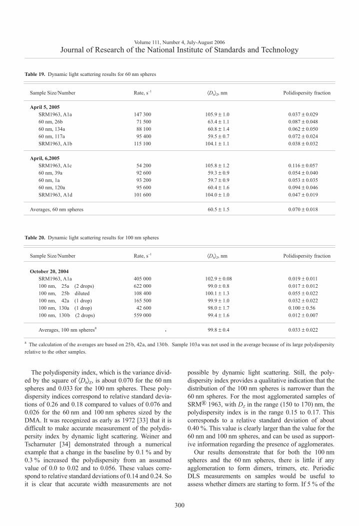
The polydispersity index, which is the variance divid-ed by the square of ⟨Dh⟩Z, is about 0.070 for the 60 nmspheres and 0.033 for the 100 nm spheres. These poly-dispersity indices correspond to relative standard devia-tions of 0.26 and 0.18 compared to values of 0.076 and0.026 for the 60 nm and 100 nm spheres sized by theDMA. It was recognized as early as 1972 [33] that it isdifficult to make accurate measurement of the polydis-persity index by dynamic light scattering. Weiner andTscharnuter [34] demonstrated through a numericalexample that a change in the baseline by 0.1 % and by0.3 % increased the polydispersity from an assumedvalue of 0.0 to 0.02 and to 0.056. These values corre-spond to relative standard deviations of 0.14 and 0.24. Soit is clear that accurate width measurements are not
possible by dynamic light scattering. Still, the poly-dispersity index provides a qualitative indication that thedistribution of the 100 nm spheres is narrower than the60 nm spheres. For the most agglomerated samples ofSRM® 1963, with DZ in the range (150 to 170) nm, thepolydispersity index is in the range 0.15 to 0.17. Thiscorresponds to a relative standard deviation of about0.40 %. This value is clearly larger than the value for the60 nm and 100 nm spheres, and can be used as support-ive information regarding the presence of agglomerates.
Our results demonstrate that for both the 100 nmspheres and the 60 nm spheres, there is little if anyagglomeration to form dimers, trimers, etc. PeriodicDLS measurements on samples would be useful to assess whether dimers are starting to form. If 5 % of the
Volume 111, Number 4, July-August 2006Journal of Research of the National Institute of Standards and Technology
300
Table 19. Dynamic light scattering results for 60 nm spheres
Sample Size/Number Rate, s–1 ⟨Dh⟩Z, nm Polidispersity fraction
April 5, 2005SRM1963, A1a 147 300 105.9 ± 1.0 0.037 ± 0.02960 nm, 26b 71 500 63.4 ± 1.1 0.087 ± 0.04860 nm, 134a 88 100 60.8 ± 1.4 0.062 ± 0.05060 nm, 117a 95 400 59.5 ± 0.7 0.072 ± 0.024SRM1963, A1b 115 100 104.1 ± 1.1 0.038 ± 0.032
April, 6,2005SRM1963, A1c 54 200 105.8 ± 1.2 0.116 ± 0.05760 nm, 39a 92 600 59.3 ± 0.9 0.054 ± 0.04060 nm, 1a 93 200 59.7 ± 0.9 0.053 ± 0.03560 nm, 120a 95 600 60.4 ± 1.6 0.094 ± 0.046SRM1963, A1d 101 600 104.0 ± 1.0 0.047 ± 0.019
Averages, 60 nm spheres 60.5 ± 1.5 0.070 ± 0.018
Table 20. Dynamic light scattering results for 100 nm spheres
Sample Size/Number Rate, s–1 ⟨Dh⟩Z, nm Polidispersity fraction
October 20, 2004SRM1963, A1a 405 000 102.9 ± 0.08 0.019 ± 0.011100 nm, 25a (2 drops) 622 000 99.0 ± 0.8 0.017 ± 0.012100 nm, 25b diluted 108 400 100.1 ± 1.3 0.055 ± 0.022100 nm, 42a (1 drop) 165 500 99.9 ± 1.0 0.032 ± 0.022100 nm, 130a (1 drop) 42 600 98.0 ± 1.7 0.100 ± 0.56100 nm, 130b (2 drops) 559 000 99.4 ± 1.6 0.012 ± 0.007
Averages, 100 nm spheresa 99.8 ± 0.4 0.033 ± 0.022
a The calculation of the averages are based on 25b, 42a, and 130b. Sample 103a was not used in the average because of its large polydispersityrelative to the other samples.
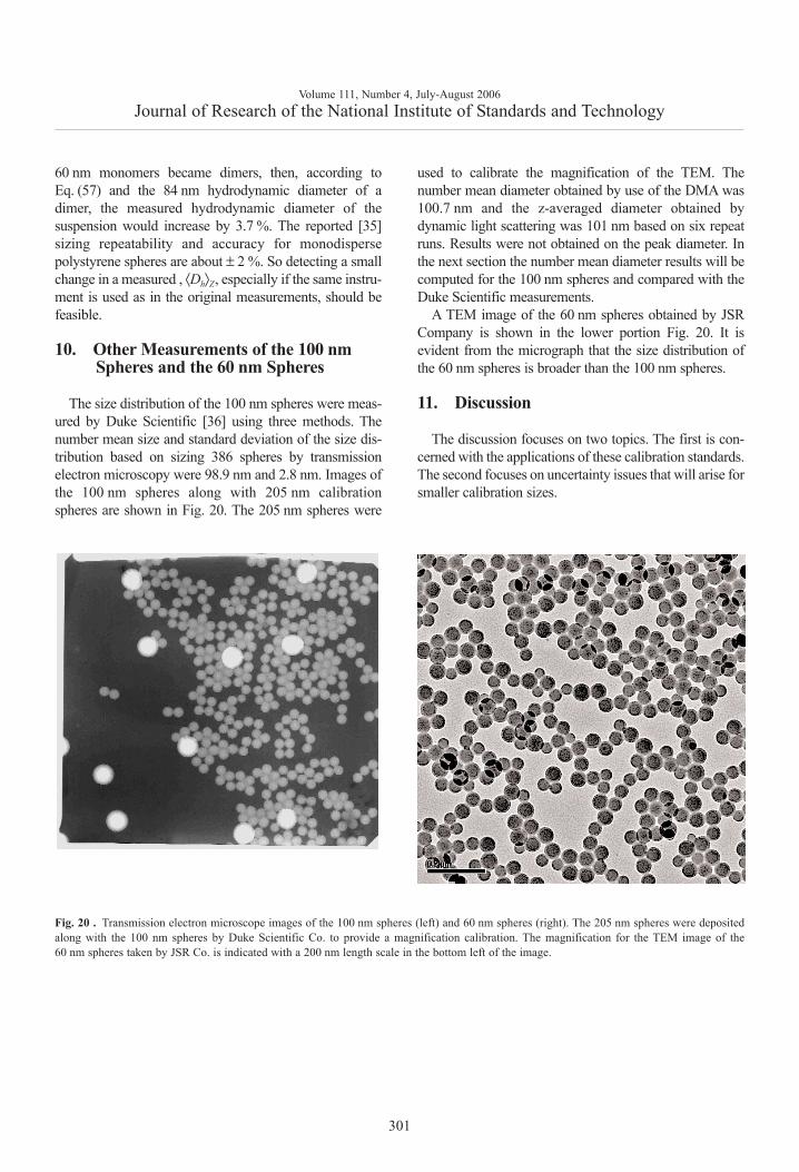
60 nm monomers became dimers, then, according toEq. (57) and the 84 nm hydrodynamic diameter of adimer, the measured hydrodynamic diameter of thesuspension would increase by 3.7 %. The reported [35]sizing repeatability and accuracy for monodispersepolystyrene spheres are about ± 2 %. So detecting a smallchange in a measured , ⟨Dh⟩Z, especially if the same instru-ment is used as in the original measurements, should befeasible.
10. Other Measurements of the 100 nmSpheres and the 60 nm Spheres
The size distribution of the 100 nm spheres were meas-ured by Duke Scientific [36] using three methods. Thenumber mean size and standard deviation of the size dis-tribution based on sizing 386 spheres by transmissionelectron microscopy were 98.9 nm and 2.8 nm. Images ofthe 100 nm spheres along with 205 nm calibration spheres are shown in Fig. 20. The 205 nm spheres were
used to calibrate the magnification of the TEM. Thenumber mean diameter obtained by use of the DMA was100.7 nm and the z-averaged diameter obtained bydynamic light scattering was 101 nm based on six repeatruns. Results were not obtained on the peak diameter. Inthe next section the number mean diameter results will becomputed for the 100 nm spheres and compared with theDuke Scientific measurements.
A TEM image of the 60 nm spheres obtained by JSRCompany is shown in the lower portion Fig. 20. It isevident from the micrograph that the size distribution ofthe 60 nm spheres is broader than the 100 nm spheres.
11. Discussion
The discussion focuses on two topics. The first is con-cerned with the applications of these calibration standards.The second focuses on uncertainty issues that will arise forsmaller calibration sizes.
Volume 111, Number 4, July-August 2006Journal of Research of the National Institute of Standards and Technology
301
Fig. 20 . Transmission electron microscope images of the 100 nm spheres (left) and 60 nm spheres (right). The 205 nm spheres were depositedalong with the 100 nm spheres by Duke Scientific Co. to provide a magnification calibration. The magnification for the TEM image of the60 nm spheres taken by JSR Co. is indicated with a 200 nm length scale in the bottom left of the image.
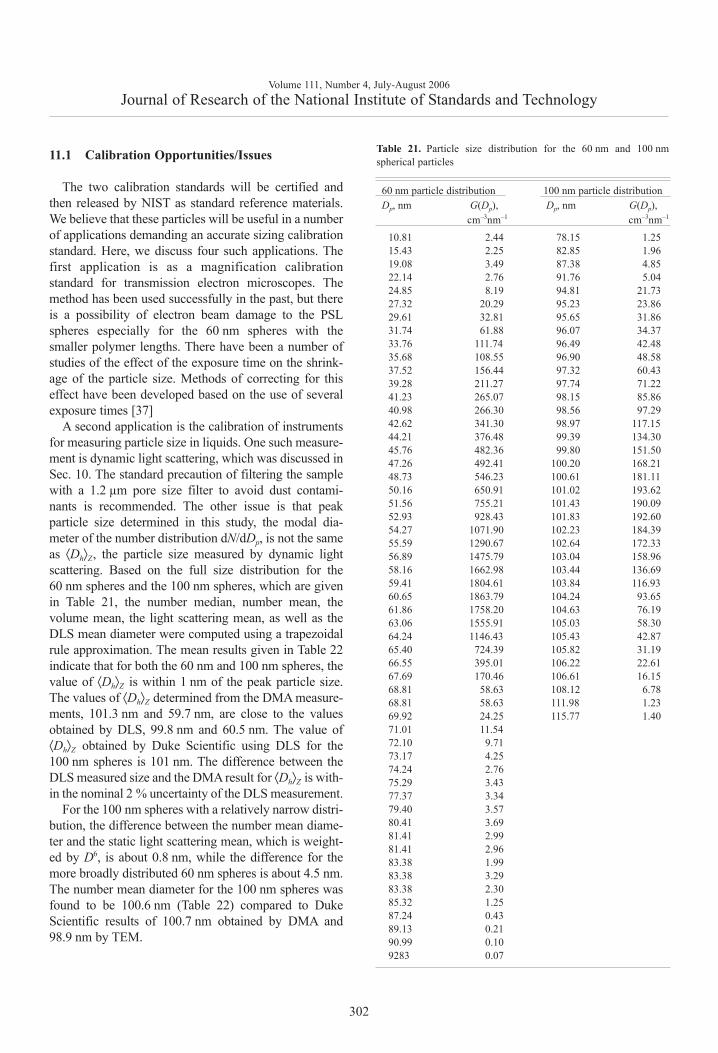
11.1 Calibration Opportunities/Issues
The two calibration standards will be certified andthen released by NIST as standard reference materials.We believe that these particles will be useful in a numberof applications demanding an accurate sizing calibrationstandard. Here, we discuss four such applications. Thefirst application is as a magnification calibrationstandard for transmission electron microscopes. Themethod has been used successfully in the past, but thereis a possibility of electron beam damage to the PSLspheres especially for the 60 nm spheres with thesmaller polymer lengths. There have been a number ofstudies of the effect of the exposure time on the shrink-age of the particle size. Methods of correcting for thiseffect have been developed based on the use of severalexposure times [37]
A second application is the calibration of instrumentsfor measuring particle size in liquids. One such measure-ment is dynamic light scattering, which was discussed inSec. 10. The standard precaution of filtering the samplewith a 1.2 µm pore size filter to avoid dust contami-nants is recommended. The other issue is that peakparticle size determined in this study, the modal dia-meter of the number distribution dN/dDp, is not the sameas ⟨Dh⟩Z, the particle size measured by dynamic lightscattering. Based on the full size distribution for the60 nm spheres and the 100 nm spheres, which are givenin Table 21, the number median, number mean, thevolume mean, the light scattering mean, as well as theDLS mean diameter were computed using a trapezoidalrule approximation. The mean results given in Table 22indicate that for both the 60 nm and 100 nm spheres, thevalue of ⟨Dh⟩Z is within 1 nm of the peak particle size.The values of ⟨Dh⟩Z determined from the DMA measure-ments, 101.3 nm and 59.7 nm, are close to the valuesobtained by DLS, 99.8 nm and 60.5 nm. The value of⟨Dh⟩Z obtained by Duke Scientific using DLS for the100 nm spheres is 101 nm. The difference between theDLS measured size and the DMA result for ⟨Dh⟩Z is with-in the nominal 2 % uncertainty of the DLS measurement.
For the 100 nm spheres with a relatively narrow distri-bution, the difference between the number mean diame-ter and the static light scattering mean, which is weight-ed by D6, is about 0.8 nm, while the difference for themore broadly distributed 60 nm spheres is about 4.5 nm.The number mean diameter for the 100 nm spheres wasfound to be 100.6 nm (Table 22) compared to DukeScientific results of 100.7 nm obtained by DMA and98.9 nm by TEM.
Volume 111, Number 4, July-August 2006Journal of Research of the National Institute of Standards and Technology
302
Table 21. Particle size distribution for the 60 nm and 100 nmspherical particles
60 nm particle distribution 100 nm particle distributionDp, nm G(Dp), Dp, nm G(Dp),
cm–3nm–1 cm–3nm–1
10.81 2.44 78.15 1.2515.43 2.25 82.85 1.9619.08 3.49 87.38 4.8522.14 2.76 91.76 5.0424.85 8.19 94.81 21.7327.32 20.29 95.23 23.8629.61 32.81 95.65 31.8631.74 61.88 96.07 34.3733.76 111.74 96.49 42.4835.68 108.55 96.90 48.5837.52 156.44 97.32 60.4339.28 211.27 97.74 71.2241.23 265.07 98.15 85.8640.98 266.30 98.56 97.2942.62 341.30 98.97 117.1544.21 376.48 99.39 134.3045.76 482.36 99.80 151.5047.26 492.41 100.20 168.2148.73 546.23 100.61 181.1150.16 650.91 101.02 193.6251.56 755.21 101.43 190.0952.93 928.43 101.83 192.6054.27 1071.90 102.23 184.3955.59 1290.67 102.64 172.3356.89 1475.79 103.04 158.9658.16 1662.98 103.44 136.6959.41 1804.61 103.84 116.9360.65 1863.79 104.24 93.6561.86 1758.20 104.63 76.1963.06 1555.91 105.03 58.3064.24 1146.43 105.43 42.8765.40 724.39 105.82 31.1966.55 395.01 106.22 22.6167.69 170.46 106.61 16.1568.81 58.63 108.12 6.7868.81 58.63 111.98 1.2369.92 24.25 115.77 1.4071.01 11.5472.10 9.7173.17 4.2574.24 2.7675.29 3.4377.37 3.3479.40 3.5780.41 3.6981.41 2.9981.41 2.9683.38 1.9983.38 3.2983.38 2.3085.32 1.2587.24 0.4389.13 0.2190.99 0.109283 0.07
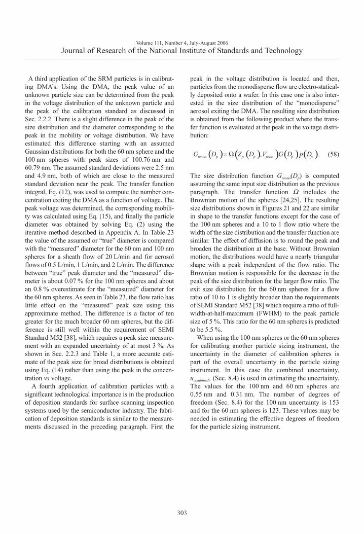
A third application of the SRM particles is in calibrat-ing DMA’s. Using the DMA, the peak value of anunknown particle size can be determined from the peakin the voltage distribution of the unknown particle andthe peak of the calibration standard as discussed inSec. 2.2.2. There is a slight difference in the peak of thesize distribution and the diameter corresponding to thepeak in the mobility or voltage distribution. We haveestimated this difference starting with an assumedGaussian distributions for both the 60 nm sphere and the100 nm spheres with peak sizes of 100.76 nm and60.79 nm. The assumed standard deviations were 2.5 nmand 4.9 nm, both of which are close to the measuredstandard deviation near the peak. The transfer functionintegral, Eq. (12), was used to compute the number con-centration exiting the DMA as a function of voltage. Thepeak voltage was determined, the corresponding mobili-ty was calculated using Eq. (15), and finally the particlediameter was obtained by solving Eq. (2) using theiterative method described in Appendix A. In Table 23the value of the assumed or “true” diameter is comparedwith the “measured” diameter for the 60 nm and 100 nmspheres for a sheath flow of 20 L/min and for aerosolflows of 0.5 L/min, 1 L/min, and 2 L/min. The differencebetween “true” peak diameter and the “measured” dia-meter is about 0.07 % for the 100 nm spheres and aboutan 0.8 % overestimate for the “measured” diameter forthe 60 nm spheres. As seen in Table 23, the flow ratio haslittle effect on the “measured” peak size using thisapproximate method. The difference is a factor of tengreater for the much broader 60 nm spheres, but the dif-ference is still well within the requirement of SEMIStandard M52 [38], which requires a peak size measure-ment with an expanded uncertainty of at most 3 %. Asshown in Sec. 2.2.3 and Table 1, a more accurate esti-mate of the peak size for broad distributions is obtainedusing Eq. (14) rather than using the peak in the concen-tration vs voltage.
A fourth application of calibration particles with asignificant technological importance is in the productionof deposition standards for surface scanning inspectionsystems used by the semiconductor industry. The fabri-cation of deposition standards is similar to the measure-ments discussed in the preceding paragraph. First the
peak in the voltage distribution is located and then,particles from the monodisperse flow are electro-statical-ly deposited onto a wafer. In this case one is also inter-ested in the size distribution of the “monodisperse”aerosol exiting the DMA. The resulting size distributionis obtained from the following product where the trans-fer function is evaluated at the peak in the voltage distri-bution:
(58)
The size distribution function Gmono(Dp) is computedassuming the same input size distribution as the previousparagraph. The transfer function Ω includes theBrownian motion of the spheres [24,25]. The resultingsize distributions shown in Figures 21 and 22 are similarin shape to the transfer functions except for the case ofthe 100 nm spheres and a 10 to 1 flow ratio where thewidth of the size distribution and the transfer function aresimilar. The effect of diffusion is to round the peak andbroaden the distribution at the base. Without Brownianmotion, the distributions would have a nearly triangularshape with a peak independent of the flow ratio. TheBrownian motion is responsible for the decrease in thepeak of the size distribution for the larger flow ratio. Theexit size distribution for the 60 nm spheres for a flowratio of 10 to 1 is slightly broader than the requirements of SEMI Standard M52 [38] which require a ratio of full-width-at-half-maximum (FWHM) to the peak particlesize of 5 %. This ratio for the 60 nm spheres is predictedto be 5.5 %.
When using the 100 nm spheres or the 60 nm spheresfor calibrating another particle sizing instrument, theuncertainty in the diameter of calibration spheres ispart of the overall uncertainty in the particle sizinginstrument. In this case the combined uncertainty,ucombined , (Sec. 8.4) is used in estimating the uncertainty.The values for the 100 nm and 60 nm spheres are0.55 nm and 0.31 nm. The number of degrees offreedom (Sec. 8.4) for the 100 nm uncertainty is 153and for the 60 nm spheres is 123. These values may beneeded in estimating the effective degrees of freedomfor the particle sizing instrument.
Volume 111, Number 4, July-August 2006Journal of Research of the National Institute of Standards and Technology
303
( ) ( )( ) ( ) ( ), .mono p p p peak p pG D Z D V G D p D= Ω

Volume 111, Number 4, July-August 2006Journal of Research of the National Institute of Standards and Technology
304
Table 22. Mean particle size based on size distribution for 100 nm and 60 nm spheres with the standard deviation of the size distribution.
Peak Diameter, nm ⟨DN⟩, nm ⟨DV⟩, nm ⟨DLS⟩, nm ⟨Dh⟩Z, nm σ ⟨DN⟩
60.55 55.70 58.49 60.23 59.72 7.90
101.52 100.61 101.05 101.43 101.31 3.97
( )( )
( ) ( )( )
( )( )
1/ 22
3
3
Number averaged diameter
Standard deviation of size distribution
Volume or mass averaged diameter of
Light scattering weighted diameter (Raleigh limit)
N
N
V
LS
DG D dDD
G D dD
D D G D dD
G D dD
DD G D dDD
D G D dD
DDD
σ
=
− =
=
=
∫∫
∫∫
∫∫
( )( )
( )
( )
6
6
6
6
11Dynamic light scattering diameter
h h hh
h h h hZ
G D dD
D G D dD
D G D dDD
D D G D dD=
∫∫
∫∫
Table 23. Comparison of DMA Diameter based on peak voltage with peak in size distribution with sheath air flow of 20 L/min
Dpeak , nm Dpeak , nm Dpeak , nm Dpeak , nm
for assumed G(Dp) Qa = 0.5 L/min Qa = 1.0 L/min Qa = 2.0 L/min
101.76 101.83 101.79 101.69
60.79 61.36 61.31 61.23
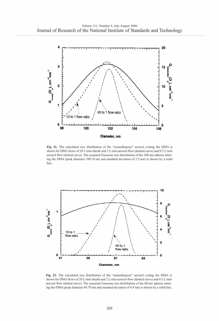
Volume 111, Number 4, July-August 2006Journal of Research of the National Institute of Standards and Technology
305
Fig. 21. The calculated size distribution of the “monodisperse” aerosol exiting the DMA isshown for DMA flows of 20 L/min sheath and 2 L/min aerosol flow (dashed curve) and 0.5 L/minaerosol flow (dotted curve). The assumed Gaussian size distribution of the 100 nm spheres enter-ing the DMA (peak diameter 100.76 nm and standard deviation of 2.5 nm) is shown by a solidline.
Fig. 22. The calculated size distribution of the “monodisperse” aerosol exiting the DMA isshown for DMA flows of 20 L/min sheath and 2 L/min aerosol flow (dashed curve) and 0.5 L/minaerosol flow (dotted curve). The assumed Gaussian size distribution of the 60 nm spheres enter-ing the DMA (peak diameter 60.79 nm and standard deviation of 4.9 nm) is shown by a solid line.

11.2 Uncertainty Issues for Smaller Particle Sizes
The uncertainty in the calibration diameter is morethan a factor of 2 larger than the next largest uncertaintyterm. Thus, an improved calibration diameter wouldreduce the overall measurement uncertainty of smallerparticles based on DMA measurements. Ehara et al. [39]measured the number average diameter of SRM® 1963and obtained a value of 100.8 nm with an expandeduncertainty of 0.66 nm compared to the NIST certifieduncertainty of 0.95 nm. Adopting the results by Eharaet al. might reduce the uncertainty in the 100 nm and60 nm PSL spheres by 20 % to 25 %.
The measurement of angle resolved light scattering byparticles on the surface [40] has resulted in an estimatedrelative combined Type B uncertainty of about 0.3 % for100 nm spheres compared to the DMA value of about0.5 %. However, there is about a 5 % difference betweenthe particle size by light scattering versus the mobilitymeasurement [41]. This difference is thought to be atleast partly a result of deformation of the particle on thesurface. Work is in progress to address this issue. Otherpromising approaches for obtaining low uncertaintiesinclude small angle x-ray scattering [42,43], field flowparticle fractionation followed by angle resolved lightscattering [44], and transmission electron microscopy[37].
Lastly we consider additional major contributors tothe uncertainty in using the DMA sizing method forsmaller particle sizes. The slip correction was not adominant uncertainty for the 60 nm and 100 nm spheresbecause of the correlation between the uncertainty in theslip correction parameter A for the unknown and for thecalibration particle. This effect will continue for particlesas small as 20 nm, but for Knudsen numbers correspon-ding to particle sizes less than about 10 nm at 101.3 kPa,the slip correction was determined using a differentcalibration particle from the one used for the largerparticles. In this case little correlation may be assumedbetween the two slip corrections.
For particle diameters smaller than 30 nm, Brownianmotion has a significant effect on the transfer function.As indicated in Table 15, the width of the transfer func-tion increases by a factor of 1.65 for a 30 nm sphere andby a factor of 3.99 for a 10 nm sphere compared to thecase with no diffusion. There is also a large decrease inthe peak of the transfer function from unity to 0.25 for the 10 nm spheres. For these cases a significant differ-ence in the measured particle size is expected comparedto the values with a triangular transfer function. The dif-fusion effects are also much greater for the flow ratio of0.025 compared to 0.10 because of the much narrower
flow volume trajectory to the outlet slit. One approachfor reducing the diffusion effect is to use a Nano-DMA,which has about an 8 fold shorter length and a correspon-ding decrease in the time available for diffusion.
12. Summary
The peak size in the number distribution of the PSLaerosol and expanded uncertainty (95 % confidencelevel) for two new nanometer range size standards ob-tained using DMA measurements are 101.8 nm ± 1.1 nmand 60.39 nm ± 0.63 nm. The estimated standard devia-tions of the size distributions are approximately 2.5 nmfor the 100 nm spheres and 4.9 nm for the 60 nmspheres. The average diameters based on numberweighting, mass weighting, light scattering weighting,and dynamic light scattering weighting are presented.
The peak mobility measurements of samples selectedat random from the 150 bottles indicate that the samplesare homogeneous. The dynamic light scattering meas-urement showed no evidence of agglomeration andprovided results consistent with the DMA measure-ments. In addition, the dynamic light scattering measure-ments will be used periodically in the future to verify thatmultimers are not forming in the samples.
Key features of the measurements to provide lowuncertainty were an accurate size calibration standard; amodified sheath/aerosol inlet, a high ratio of the sheathflow to the aerosol flow (40 to 1), and a recirculatingsheath flow; the use of the transfer function integral inthe calibration process and in validating the accuracy ofthe inferred peak particle size; accurate pressure, temper-ature, and voltage instrumentation; the use of electro-spray to avoid multimers and reduce the effect of non-volatile residue for the 60 nm spheres; correcting for thelinear drift in the concentration produced by the electro-spray and accounting for the presence of doubletproduced by the pneumatic nebulizer. An importantconsideration in the uncertainty analysis was the correla-tion between the slip correction of the calibrationparticle and the measured particle. This reduced theexpanded uncertainty from about 1.8 % of the particlesize to about 1.0 %.
The peak diameter is for the PSL spheres as anaerosol. The contaminants in the PSL suspension resultin a residue layer on the spheres. The estimated thicknessof this layer is 0.30 nm for the 100 nm spheres and0.03 nm for the 60 nm spheres. The layer thickness for afixed particle suspension was shown to be stronglydependent on the method of generating the aerosol. Thechange in layer thickness for the SRM® 1963 spheresfor the different generators resulted in a change in the
Volume 111, Number 4, July-August 2006Journal of Research of the National Institute of Standards and Technology
306
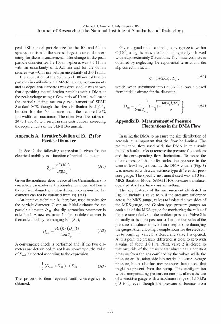
peak PSL aerosol particle size for the 100 and 60 nmspheres and is also the second largest source of uncer-tainty for these measurements. The change in the peakparticle diameter for the 100 nm spheres was + 0.11 nmwith an uncertainty of ± 0.21 nm and for the 60 nmspheres was – 0.11 nm with an uncertainty of ± 0.19 nm.
The application of the 60 nm and 100 nm calibrationparticles in calibrating a DMA for sizing measurementsand as deposition standards was discussed. It was shownthat depositing the calibration particles with a DMA atthe peak voltage using a flow ratio of 10 to 1 will meetthe particle sizing accuracy requirement of SEMIStandard M52 though the size distribution is slightlybroader for the 60 nm case than the required 5 %full-width-half-maximum. The other two flow ratios of20 to 1 and 40 to 1 result in size distributions exceedingthe requirements of the SEMI Document.
Appendix A. Iterative Solution of Eq. (2) forParticle Diameter
In Sec. 2, the following expression is given for theelectrical mobility as a function of particle diameter:
(A1)
Given the nonlinear dependence of the Cunningham slipcorrection parameter on the Knudsen number, and hencethe particle diameter, a closed form expression for thediameter can not be obtained from Eq. (A1).
An iterative technique is, therefore, used to solve forthe particle diameter. Given an initial estimate for theparticle diameter, Dold , the slip correction parameter iscalculated. A new estimate for the particle diameter isthen calculated by rearranging Eq. (A1),
(A2)
A convergence check is performed and, if the two dia-meters are determined to not have converged, the valueof Dold is updated according to the expression,
(A3)
The process is then repeated until convergence isobtained.
Given a good initial estimate, convergence to withinO(10–7) using the above technique is typically achievedwithin approximately 8 iterations. The initial estimate isobtained by neglecting the exponential term within theslip correction factor.
(A4)
which, when substituted into Eq. (A1), allows a closedform initial estimate for the diameter,
(A5)
Appendix B. Measurement of PressureFluctuations in the DMA Flow
In using the DMA to measure the size distribution ofaerosols it is important that the flow be laminar. Therecirculation flow used with the DMA in this studyincludes buffer tanks to remove the pressure fluctuationsand the corresponding flow fluctuations. To assess theeffectiveness of the buffer tanks, the pressure in theexcess flow line just outside the DMA chassis (Fig. 3)was measured with a capacitance type differential pres-sure gauge. The specific instrument used was a 10 torrMKS Baratron Model 698A11TRA pressure transduceroperated at a 1 ms time constant setting.
The key features of the measurement illustrated inFig. 23 include a valve to null the pressure differenceacross the MKS gauge, valves to isolate the two sides ofthe MKS gauge, and Gardon type pressure gauges oneach side of the MKS gauge for monitoring the value ofthe pressure relative to the ambient pressure. Valve 2 isnormally in the open position to short the two sides of thepressure transducer to avoid an overpressure damagingthe gauge. After allowing a couple hours for the electron-ics to warm up, valve 3 is closed and valve 1 is opened.At this point the pressure difference is close to zero witha value of about ± 0.1 Pa. Next, valve 2 is closed sothat one side of the pressure transducer has a constantpressure from the gas confined by the valves while thepressure on the other side has nearly the same averagepressure, but it also has any pressure fluctuations thatmight be present from the pump. This configurationwith a compensating pressure on one side allows the useof a sensitive gauge with a maximum range of 1.33 kPa(10 torr) even though the pressure difference from
Volume 111, Number 4, July-August 2006Journal of Research of the National Institute of Standards and Technology
307
( ).
3pp
eC KnZ
Dπµ=
( )( )oldnew .
3 p
eC Kn DD
Zπµ=
( )new old old1 .2
D D D+ →
11 2 / ,pC A Dλ= +
1init
61 1 .
6p
p
A ZeDZ e
π λµπµ
= + +

ambient is as large as 2.7 kPa. The pressure data is typi-cally collected at a speed of 1 kHz for 10 s.
Four sets of measurements were carried out. In thefirst set the pressure gauge was connected to the systemin its normal configuration with a recirculating flow of20 L/min. In this case the average pressure at the inletside of the pump is – 1.7 kPa relative to the ambientpressure. In the second set, a nitrogen gas cylinder isused to provide a steady flow of 20 L/min through theDMA. In this case the cylinder flow is connected to thesheath flow inlet and the excess flow to an exhaust line.The recirculating system is disconnected from the flow.This measurement was performed to observe the pres-sure fluctuations for a steady flow. In this case, theaverage pressure is about 0.61 kPa above ambient. Thefluctuations from the pump are observed in the third setof experiments by connecting the outlet of the twopumps (Thomas 107 CAB18 diaphragm type) to thepressure transducer. In this case the average pressure is2.7 kPa above ambient. In all three cases, the 0.79 cm(5/16 in) ID tubing was unobstructed for at least40 diameter before and after the tee for the pressuremeasurement. The 60 cm of tubing and connectors/valves between the gauge and the pressure transducerwere identical for the steady flow and the recirculatingflow. For the pump measurements, the length of tubingwas increased by about 25 cm. The fourth measurementwas with no flow with valve’s 1 and 3 closed and 2 open. It was designed to measure the electronic nose of thegauge.
The electronic noise was small with a standard devia-tion based on 1 s of data of about 0.25 Pa. The pressurefluctuation from the pump has a distinct frequency ofabout 29 Hz and with an amplitude in excess of± 1333 Pa (10 torr) as shown in Fig. 24. There is a sec-ondary peak occurring at the same frequency. The pres-sure fluctuation for the recirculating flow appear to cor-relate somewhat with the pressure peaks including thesecondary peaks for the pump alone as indicated inFig. 24. The nominal magnitude of the fluctuations isabout 5 Pa about the mean which is at least 270 timessmaller than the amplitude of the pump pressure.
The pressure fluctuation for the steady flow from thecylinder appear less regular than for the recirculatingflow as shown in Fig. 25. The standard deviation of thepressure for a 1 s time period for the steady flow is about3.7 Pa compared to a value of about 5.1 Pa for the recir-culating flow. The fluctuations in the buffered flow isgreatly reduced relative to the pump flow though thefluctuation pattern is more regular than for the steadyflow and the noise level as indicated by the standarddeviation is about 40 % larger than the steady flow.
To provide more quantitative information of thepresence of characteristic frequencies, the power spectrafor the pressure data were computed. Before computingthe power spectrum, the average value of the pres-sure was subtracted from the pressure data so thatthe analysis was carried out for Pv , the variation aboutthe mean. The fast Fourier transform, C(k), was com-puted from the time sequence, and from this the
Volume 111, Number 4, July-August 2006Journal of Research of the National Institute of Standards and Technology
308
Fig. 23. Experimental set up for the pressure measurements.
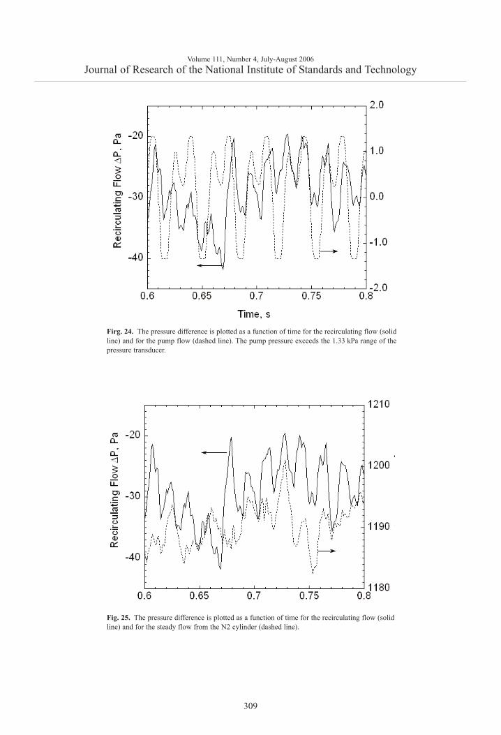
Volume 111, Number 4, July-August 2006Journal of Research of the National Institute of Standards and Technology
309
Firg. 24. The pressure difference is plotted as a function of time for the recirculating flow (solidline) and for the pump flow (dashed line). The pump pressure exceeds the 1.33 kPa range of thepressure transducer.
Fig. 25. The pressure difference is plotted as a function of time for the recirculating flow (solidline) and for the steady flow from the N2 cylinder (dashed line).

norm of the amplitude was determined as a function offrequency.
(B1)
The quantity k is a dimensionless frequency, which isrelated to frequency f by the following expression:
(B2)
There were 4092 points data points analyzed and thetime increment ∆t was 0.001 s. The normalization inEq. (B1) is such that the sum of the values of Π
∧
(k)is ameasure of the variance of the pressure signal.
The power spectra plotted in Fig. 26 all have peaksnear 30 Hz (28.7) and near 60 Hz (57.9). The power isabout 1.0 × 10⁵ larger amplitude than for the recircula-tion flow. This again shows that the amplitude is great-ly diminished for the recirculation flow. This result isconsistent with the pressure measurements, since thepower is proportional to the square of the pressureamplitude. The peaks near 30 Hz and 60 Hz for thenitrogen tank flow are surprising since the pump is notin the system. We do not have an explanation for thisobservation.
Acknowledgement
Scott R. Kukuck was supported as a NationalResearch Council Postdoctoral Fellow at NIST whileassisting with this study. Jiann C. Yang assisted withfigures and computer programming. The authors thankStanley Kaufman from TSI Inc. for his insightful com-ments about the manuscript.
Volume 111, Number 4, July-August 2006Journal of Research of the National Institute of Standards and Technology
310
( ) ( )( )22ˆ 0 0 /C NΠ =
( ) ( )( )22ˆ 2 / for 1,2, , ( / 2 1)k C k N k NΠ = = −…
( ) ( )( )22ˆ / 2 / .k N C k NΠ = =
( )/ 4092 .f k t∆=
Fig 26-upper. The power spectra obtained from the pressure dataare plotted for the pump flow(upper), for the recirculating flow(middle), and for flow from a N2 cylinder (lower). In all three casesthe same two characteristic frequencies of 29 Hz and 58 Hz appear.
Fig 26-middle. The power spectra obtained from the pressure dataare plotted for the pump flow(upper), for the recirculating flow(middle), and for flow from a N2 cylinder (lower). In all three casesthe same two characteristic frequencies of 29 Hz and 58 Hz appear.
Fig 26-lower. The power spectra obtained from the pressure data areplotted for the pump flow(upper), for the recirculating flow(middle), and for flow from a N2 cylinder (lower). In all three casesthe same two characteristic frequencies of 29 Hz and 58 Hz appear.
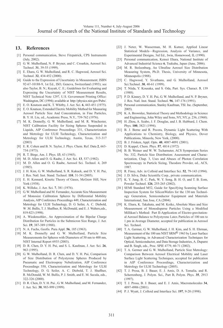
13. References[1] Personal communication, Steve Fitzpatrick, CPS Instruments
(July, 2002).[2] G. W. Mulholland, N. P. Bryner, and C. Croarkin, Aerosol Sci.
Technol. 31, 39-55 (1999).[3] E. Ehara, G. W. Mulholland, and R. C. Hagwood, Aerosol Sci.
Technol. 32, 434-452 (2000).[4] Guide to the Expression of Uncertainty in Measurement; ISBN
92-67-10188-9, 1st Ed., ISO, Geneva, Switzerland (1993); seealso Taylor, B. N.; Kuyatt, C. E.; Guidelines for Evaluating andExpressing the Uncertainty of NIST Measurement Results,NIST Technical Note 1297, U.S. Government Printing Office:Washington, DC (1994); available at http://physics.nist.gov/Pubs/.
[5] E. O. Knutson and K. T. Whitby, J. Aer. Sci. 6, 443-451 (1975).[6] E. O. Knutson, Extended Electric Mobility Method for Measuring
Aerosol Particle Size And Concentration, in Fine Particles,B. Y. H. Liu, ed., Academic Press, N.Y., 739-762 (1976).
[7] M. K. Donnelly, G. W. Mulholland, and M. R. Winchester,NIST Calibration Facility for Sizing Spheres Suspended inLiquids, AIP Conference Proceedings 331, Characterizationand Metrology for ULSI Technology, Characterization andMetrology for ULSI Technology, Austin, Texas, 313-317(2003)
[8] E. R. Cohen and B. N. Taylor, J. Phys. Chem. Ref. Data 2, 663-734 (1973).
[9] R. T. Birge, Am. J. Phys. 13, 63 (1945).[10] M. D. Allen and O. G. Raabe, J. Aer. Sci. 13, 537 (1982).[11] M. D. Allen and O. G. Raabe, Aerosol Sci. Technol. 4, 269
(1985).[12] J. H. Kim, G. W. Mulholland, S. R. Kukuck, and D. Y. H. Pui,
J. Res. Natl. Inst. Stand. Technol. 110, 31-54 (2005).[13] E. H. Kennard, Kinetic Theory of Gases, McGraw Hill, New
York (1938).[14] K. Willeke, J. Aer. Sci. 7, 381 (1976).[15] G. W. Mulholland and M. Fernandez, Accurate Size Measurement
of Monosize Calibration Spheres by Differential MobilityAnalysis, AIP Conference Proceedings 449, Characterization andMetrology for ULSI Technology, D. G Seiler, A. C. Diebold,W .M. Bullis, T. J. Shaffner, R. McDonald, and E. J. Walters,eds.,819-823 (1998).
[16] A. Wiedensohler., An Approximation of the Bipolar ChargeDistribution for Particles in the Submicron Size Range, J. Aer.Sci. 19, 387-389 (1988).
[17] N. A. Fuchs, Geofis. Pura Appl. 56, 185 (1963).[18] M. K. Donnelly and G. W. Mulholland, Particle Size
Measurements for Spheres with Diameters of 50 nm to 400 nm,NIST Internal Report 6935 (2003).
[19] D. R. Chen, D. Y. H. Pui, and S. L. Kaufman, J. Aer. Sci. 26,963 (1995).
[20] G. W. Mulholland, D. R. Chen, and D. Y. H. Pui, Comparisonof Size Distribution of Polystyrene Spheres Produced byPneumatic and Electrospray Nebulization, AIP ConferenceProceedings 550, Characterization and Metrology for ULSITechnology, D. G. Seiler, A. C. Diebold, T. J. Shaffner,R. McDonald, W. M. Bullis, P. J. Smith, and E. M. Secula, eds.,322-326 (2000).
[21] D. R. Chen, D. Y. H. Pui , G. W. Mulholland, and M. Fernandez,J. Aer. Sci. 30, 983-999 (1999).
[22] J. Neter, W. Wasserman, M. H. Kutner, Applied LinearStatistical Models—Regression, Analysis of Variance, andExperimental Designs, 3rd Ed., Iwin, Homewood, IL (1990).
[23] Personal communication, Kensei Ehara, National Institute ofAdvanced Industrial Science 6, Tsukuba, Japan (June, 2006).
[24] M. R. Stolzenburg, An Ultrafine Aerosol Size DistributionMeasuring System, Ph.D. Thesis, University of Minnesota,Minneapolis (1988).
[25] C. Hagwood, Y. Sivathanu, and G. Mulholland, AerosolSci.Technol. 30, 40-61 (1999).
[26] T. Niida, Y. Kousaka, and S. Oda, Part. Sys. Charact. 5, 139(1988).
[27] P. D. Kinney, D. Y. H. Pui, G. W. Mulholland, and N. P. Bryner,J. Res. Natl. Inst. Stand. Technol. 96, 147-176 (1991).
[28] Personal communication, Stanley Kaufman, TSI. Inc. (September,2005).
[29] K. A. Brownlee, Statistical Theory and Methodology in Scienceand Engineering, John Wiley and Sons, NY, NY, p. 236, (1960).
[30] H. Zhou, A. Szabo, J. F. Douglas, and J. B. Hubbard, J. Chem.Phys. 100, 3821 (1994).
[31] B. J. Berne and R. Pecora, Dynamic Light Scattering WithApplications to Chemistry, Biology, and Physics, DoverPublications, Mineola, New York, (2000).
[32] B. J. Frisken, Appl. Opts. 40, 4087-4091 (2001).[33] D. Koppel, Chem. Phys. 57, 4814 (1972)[34] B. B. Weiner and W. W. Tscharnuter, ACS Symposium Series
No. 332, Particle Size Distribution: Assessment and Charac-terization, Chap. 3, Uses and Abuses of Photon CorrelationSpectroscopy in Particle Sizing, Theodore Provder, ed., ACS,1987.
[35] R. Finsy, Adv. in Colloid and Interface Sci. 52, 79-143 (1994).[36] J. D. Silva, Duke Scientific Corp., private communication.[37] K. Y. Jung, B. C. Park, W. Y. Song, B. H. O, and T. B. Eom,
Powder Technol. 126, 255-265 (2002).[38 ] SEMI Standard M52, Guide for Specifying Scanning Surface
Inspection System for SiliconWafers for the 130 nm Technol-ogy Generation, Semiconductor Equipment and MaterialsInternational, San Jose, CA (2004).
[39] K. Ehara, K. Takahata, and M. Koike, Absolute Mass and SizeMeasurement of Monodisperse Particles Using a ModifiedMillikan’s Method: Part II-Application of Electro-gravitation-al Aerosol Balance to Polystyrene Latex Particles of 100 nm to1 pm in Average Diameter, accepted for publication in AerosolSci. Technol.
[40] T. A. Germer, G. W. Mulholland, J. H. Kim, and S. H. Ehrman,Measurement of the 100 nm NIST SRM® 1963 by Laser SurfaceLight Scattering, in Advanced Characterization Techniques forOptical, Semiconductor, and Data Storage Industries, A. Duparreand B. Singh, eds., Proc. SPIE 4779, 60-71 (2002).
[41] T. A. Germer and G. W. Mulholland, Particle Size Metrology:Comparison Between Aerosol Electrical Mobility and LaserSurface Light Scattering Techniques, accepted for publicationin AIP Conference Proceedings, Characterization andMetrology for ULSI Technology (2005).
[42] T. J. Prosa, B. J. Bauer, E. J. Amis, D. A. Tomalia, and R.Scherrenberg, J. Polym. Sci., Part B, Polym. Phys. 35, 2913(1997).
[43] T. J. Prosa, B. J. Bauer, and E. J. Amis, Macromolecules 34,4897-4906 (2001).
[44] P. J. Wyatt, J. Colloid and Interface Sci. 197, 9-20 (1998).
Volume 111, Number 4, July-August 2006Journal of Research of the National Institute of Standards and Technology
311

About the authors: George W. Mulholland is a VisitingProfessor at the University of Maryland after 32 years atNIST. He is continuing his research on nanoparticlemetrology and smoke properties/smoke detection.
Michelle K. Donnelly is a fire protection engineerworking in the Fire Research Division of the NISTBuilding and Fire Research Laboratory. Her researchareas include thermal environment measurements andparticle sizing metrology.
Charles R. Hagwood is a mathematical statistician inthe NIST Statistical Engineering Division where heconsults on statistical data analysis and stochasticmodeling.
Scott R. Kukuck was a National Research CouncilPostdoctoral Research Associate in the Fire ResearchDivision in the NIST Building and Fire ResearchLaboratory while doing this work. He is currently work-ing as a mechanical engineer at the Army ResearchLaboratory.
Vincent A. Hackley is a research chemist in theCeramics Division of the NIST Materials Science andEngineering Laboratory, where he is the leader of theNanoparticle Metrology for Biomedical Applicationsproject
David Y. H. Pui is a Distinguished McKnightUniversity Professor at the University of Minnesota,Minneapolis. He is Director of the Particle TechnologyLaboratory in the Mechanical Engineering Department.
The National Institute of Standards and Technology isan agency of the Technology Administration, U.S.Department of Commerce.
Volume 111, Number 4, July-August 2006Journal of Research of the National Institute of Standards and Technology
312