10. mechanical springs 501 companies, 2008...
TRANSCRIPT

Budynas−Nisbett: Shigley’s
Mechanical Engineering
Design, Eighth Edition
III. Design of Mechanical
Elements
10. Mechanical Springs 501© The McGraw−Hill
Companies, 2008
10 Mechanical Springs
Chapter Outline
10–1 Stresses in Helical Springs 500
10–2 The Curvature Effect 501
10–3 Deflection of Helical Springs 502
10–4 Compression Springs 502
10–5 Stability 504
10–6 Spring Materials 505
10–7 Helical Compression Spring Design for Static Service 510
10–8 Critical Frequency of Helical Springs 516
10–9 Fatigue Loading of Helical Compression Springs 518
10–10 Helical Compression Spring Design for Fatigue Loading 521
10–11 Extension Springs 524
10–12 Helical Coil Torsion Springs 532
10–13 Belleville Springs 539
10–14 Miscellaneous Springs 540
10–15 Summary 542
499

Budynas−Nisbett: Shigley’s
Mechanical Engineering
Design, Eighth Edition
III. Design of Mechanical
Elements
10. Mechanical Springs502 © The McGraw−Hill
Companies, 2008
500 Mechanical Engineering Design
When a designer wants rigidity, negligible deflection is an acceptable approximation as
long as it does not compromise function. Flexibility is sometimes needed and is often
provided by metal bodies with cleverly controlled geometry. These bodies can exhibit
flexibility to the degree the designer seeks. Such flexibility can be linear or nonlinear
in relating deflection to load. These devices allow controlled application of force or
torque; the storing and release of energy can be another purpose. Flexibility allows tem-
porary distortion for access and the immediate restoration of function. Because of
machinery’s value to designers, springs have been intensively studied; moreover, they
are mass-produced (and therefore low cost), and ingenious configurations have been
found for a variety of desired applications. In this chapter we will discuss the more fre-
quently used types of springs, their necessary parametric relationships, and their design.
In general, springs may be classified as wire springs, flat springs, or special-shaped
springs, and there are variations within these divisions. Wire springs include helical
springs of round or square wire, made to resist and deflect under tensile, compressive,
or torsional loads. Flat springs include cantilever and elliptical types, wound motor- or
clock-type power springs, and flat spring washers, usually called Belleville springs.
10–1 Stresses in Helical SpringsFigure 10–1a shows a round-wire helical compression spring loaded by the axial force F.
We designate D as the mean coil diameter and d as the wire diameter. Now imagine
that the spring is cut at some point (Fig. 10–1b), a portion of it removed, and the effect
of the removed portion replaced by the net internal reactions. Then, as shown in the
figure, from equilibrium the cut portion would contain a direct shear force F and a tor-
sion T = F D/2.
To visualize the torsion, picture a coiled garden hose. Now pull one end of the
hose in a straight line perpendicular to the plane of the coil. As each turn of hose is
pulled off the coil, the hose twists or turns about its own axis. The flexing of a helical
spring creates a torsion in the wire in a similar manner.
The maximum stress in the wire may be computed by superposition of the direct
shear stress given by Eq. (3–23), p. 85, and the torsional shear stress given by Eq. (3–37),
p. 96. The result is
τmax = T r
J+ F
A(a)
d
F F
F
F
T = FD�2
D
(a)
(b)
Figure 10–1
(a) Axially loaded helicalspring; (b) free-body diagramshowing that the wire issubjected to a direct shearand a torsional shear.

Budynas−Nisbett: Shigley’s
Mechanical Engineering
Design, Eighth Edition
III. Design of Mechanical
Elements
10. Mechanical Springs 503© The McGraw−Hill
Companies, 2008
Mechanical Springs 501
1Cyril Samónov, “Some Aspects of Design of Helical Compression Springs,” Int. Symp. Design and
Synthesis, Tokyo, 1984.
at the inside fiber of the spring. Substitution of τmax = τ , T = F D/2, r = d/2, J =πd4/32, and A = πd2/4 gives
τ = 8F D
πd3+ 4F
πd2(10–1)
Now we define the spring index
C = D
d(10–2)
which is a measure of coil curvature. With this relation, Eq. (10–1) can be rearranged
to give
τ = Ks
8F D
πd3(10–3)
where Ks is a shear-stress correction factor and is defined by the equation
Ks = 2C + 1
2C(10–4)
For most springs, C ranges from about 6 to 12. Equation (10–3) is quite general and
applies for both static and dynamic loads.
The use of square or rectangular wire is not recommended for springs unless
space limitations make it necessary. Springs of special wire shapes are not made in
large quantities, unlike those of round wire; they have not had the benefit of refining
development and hence may not be as strong as springs made from round wire. When
space is severely limited, the use of nested round-wire springs should always be con-
sidered. They may have an economical advantage over the special-section springs, as
well as a strength advantage.
10–2 The Curvature EffectEquation (10–1) is based on the wire being straight. However, the curvature of the wire
increases the stress on the inside of the spring but decreases it only slightly on the out-
side. This curvature stress is primarily important in fatigue because the loads are lower
and there is no opportunity for localized yielding. For static loading, these stresses can
normally be neglected because of strain-strengthening with the first application of load.
Unfortunately, it is necessary to find the curvature factor in a roundabout way. The
reason for this is that the published equations also include the effect of the direct shear
stress. Suppose Ks in Eq. (10–3) is replaced by another K factor, which corrects for
both curvature and direct shear. Then this factor is given by either of the equations
KW = 4C − 1
4C − 4+ 0.615
C(10–5)
K B = 4C + 2
4C − 3(10–6)
The first of these is called the Wahl factor, and the second, the Bergsträsser factor.1
Since the results of these two equations differ by less than 1 percent, Eq. (10–6) is

Budynas−Nisbett: Shigley’s
Mechanical Engineering
Design, Eighth Edition
III. Design of Mechanical
Elements
10. Mechanical Springs504 © The McGraw−Hill
Companies, 2008
502 Mechanical Engineering Design
2For a thorough discussion and development of these relations, see Cyril Samónov, “Computer-Aided
Design of Helical Compression Springs,” ASME paper No. 80-DET-69, 1980.
preferred. The curvature correction factor can now be obtained by canceling out the
effect of the direct shear. Thus, using Eq. (10–6) with Eq. (10–4), the curvature cor-
rection factor is found to be
Kc = K B
Ks
= 2C(4C + 2)
(4C − 3)(2C + 1)(10–7)
Now, Ks , K B or KW , and Kc are simply stress correction factors applied multiplica-
tively to T r/J at the critical location to estimate a particular stress. There is no stress
concentration factor. In this book we will use τ = K B(8F D)/(πd3) to predict the
largest shear stress.
10–3 Deflection of Helical SpringsThe deflection-force relations are quite easily obtained by using Castigliano’s theorem.
The total strain energy for a helical spring is composed of a torsional component and
a shear component. From Eqs. (4–16) and (4–17), p. 156, the strain energy is
U = T 2l
2G J+ F2l
2AG(a)
Substituting T = F D/2, l = π DN , J = πd4/32, and A = πd2/4 results in
U = 4F2 D3 N
d4G+ 2F2 DN
d2G(b)
where N = Na = number of active coils. Then using Castigliano’s theorem, Eq. (4–20),
p. 158, to find total deflection y gives
y = ∂U
∂ F= 8F D3 N
d4G+ 4F DN
d2G(c)
Since C = D/d , Eq. (c) can be rearranged to yield
y = 8F D3 N
d4G
(
1 + 1
2C2
)
.= 8F D3 N
d4G(10–8)
The spring rate, also called the scale of the spring, is k = F/y, and so
k.= d4G
8D3 N(10–9)
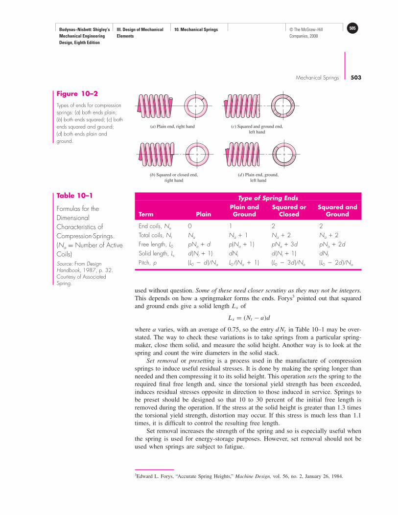
10–4 Compression SpringsThe four types of ends generally used for compression springs are illustrated in Fig. 10–2.
A spring with plain ends has a noninterrupted helicoid; the ends are the same as if a
long spring had been cut into sections. A spring with plain ends that are squared or
closed is obtained by deforming the ends to a zero-degree helix angle. Springs should
always be both squared and ground for important applications, because a better transfer
of the load is obtained.
Table 10–1 shows how the type of end used affects the number of coils and the
spring length.2 Note that the digits 0, 1, 2, and 3 appearing in Table 10–1 are often
Budynas−Nisbett: Shigley’s
Mechanical Engineering
Design, Eighth Edition
III. Design of Mechanical
Elements
10. Mechanical Springs 505© The McGraw−Hill
Companies, 2008
Mechanical Springs 503
(a) Plain end, right hand (c) Squared and ground end,
left hand
(b) Squared or closed end,
right hand
(d ) Plain end, ground,
left hand
+ +
+ +
Figure 10–2
Types of ends for compressionsprings: (a) both ends plain;(b) both ends squared; (c) bothends squared and ground;(d) both ends plain andground.
Type of Spring Ends
Plain and Squared or Squared andTerm Plain Ground Closed Ground
End coils, Ne 0 1 2 2
Total coils, Nt Na Na � 1 Na � 2 Na � 2
Free length, L0 pNa � d p(Na � 1) pNa � 3d pNa � 2d
Solid length, Ls d (Nt � 1) dNt d (Nt � 1) dNt
Pitch, p (L0 � d ) Na L0 (Na � 1) (L0 � 3d ) Na (L0 � 2d ) Na
Table 10–1
Formulas for the
Dimensional
Characteristics of
Compression-Springs.
(Na = Number of Active
Coils)
Source: From DesignHandbook, 1987, p. 32.Courtesy of AssociatedSpring.
3Edward L. Forys, “Accurate Spring Heights,” Machine Design, vol. 56, no. 2, January 26, 1984.
used without question. Some of these need closer scrutiny as they may not be integers.
This depends on how a springmaker forms the ends. Forys3 pointed out that squared
and ground ends give a solid length Ls of
Ls = (Nt − a)d
where a varies, with an average of 0.75, so the entry d Nt in Table 10–1 may be over-
stated. The way to check these variations is to take springs from a particular spring-
maker, close them solid, and measure the solid height. Another way is to look at the
spring and count the wire diameters in the solid stack.
Set removal or presetting is a process used in the manufacture of compression
springs to induce useful residual stresses. It is done by making the spring longer than
needed and then compressing it to its solid height. This operation sets the spring to the
required final free length and, since the torsional yield strength has been exceeded,
induces residual stresses opposite in direction to those induced in service. Springs to
be preset should be designed so that 10 to 30 percent of the initial free length is
removed during the operation. If the stress at the solid height is greater than 1.3 times
the torsional yield strength, distortion may occur. If this stress is much less than 1.1
times, it is difficult to control the resulting free length.
Set removal increases the strength of the spring and so is especially useful when
the spring is used for energy-storage purposes. However, set removal should not be
used when springs are subject to fatigue.

Budynas−Nisbett: Shigley’s
Mechanical Engineering
Design, Eighth Edition
III. Design of Mechanical
Elements
10. Mechanical Springs506 © The McGraw−Hill
Companies, 2008
504 Mechanical Engineering Design
4Cyril Samónov “Computer-Aided Design,” op. cit.
5A. M. Wahl, Mechanical Springs, 2d ed., McGraw-Hill, New York, 1963.
6J. A. Haringx, “On Highly Compressible Helical Springs and Rubber Rods and Their Application for
Vibration-Free Mountings,” I and II, Philips Res. Rep., vol. 3, December 1948, pp. 401–449, and vol. 4,
10–5 StabilityIn Chap. 4 we learned that a column will buckle when the load becomes too large.
Similarly, compression coil springs may buckle when the deflection becomes too
large. The critical deflection is given by the equation
ycr = L0C ′1
[
1 −(
1 − C ′2
λ2eff
)1/2]
(10–10)
where ycr is the deflection corresponding to the onset of instability. Samónov4 states that
this equation is cited by Wahl5 and verified experimentally by Haringx.6 The quantity
λeff in Eq. (10–10) is the effective slenderness ratio and is given by the equation
λeff = αL0
D(10–11)
C ′1 and C ′
2 are elastic constants defined by the equations
C ′1 = E
2(E − G)
C ′2 = 2π2(E − G)
2G + E
Equation (10–11) contains the end-condition constant α. This depends upon how the
ends of the spring are supported. Table 10–2 gives values of α for usual end conditions.
Note how closely these resemble the end conditions for columns.
Absolute stability occurs when, in Eq. (10–10), the term C ′2/λ
2eff is greater than
unity. This means that the condition for absolute stability is that
L0 <π D
α
[
2(E − G)
2G + E
]1/2
(10–12)
End Condition Constant
Spring supported between flat parallel surfaces (fixed ends) 0.5
One end supported by flat surface perpendicular to spring axis (fixed);other end pivoted (hinged) 0.707
Both ends pivoted (hinged) 1
One end clamped; other end free 2
∗Ends supported by flat surfaces must be squared and ground.
Table 10–2
End-Condition
Constants α for Helical
Compression Springs*
February 1949, pp. 49–80

Budynas−Nisbett: Shigley’s
Mechanical Engineering
Design, Eighth Edition
III. Design of Mechanical
Elements
10. Mechanical Springs 507© The McGraw−Hill
Companies, 2008
Mechanical Springs 505
For steels, this turns out to be
L0 < 2.63D
α(10–13)
For squared and ground ends α = 0.5 and L0 < 5.26D.
10–6 Spring MaterialsSprings are manufactured either by hot- or cold-working processes, depending upon
the size of the material, the spring index, and the properties desired. In general, pre-
hardened wire should not be used if D/d < 4 or if d > 14
in. Winding of the spring
induces residual stresses through bending, but these are normal to the direction of the
torsional working stresses in a coil spring. Quite frequently in spring manufacture,
they are relieved, after winding, by a mild thermal treatment.
A great variety of spring materials are available to the designer, including plain
carbon steels, alloy steels, and corrosion-resisting steels, as well as nonferrous materi-
als such as phosphor bronze, spring brass, beryllium copper, and various nickel alloys.
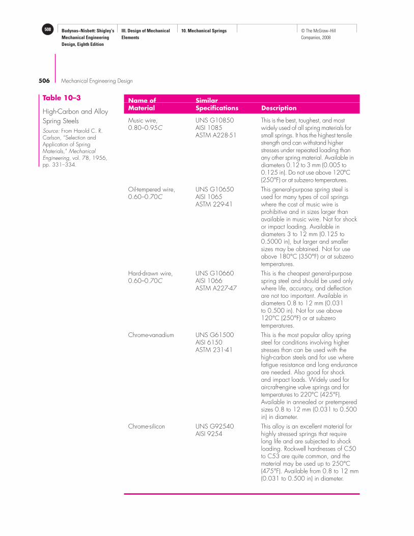
Descriptions of the most commonly used steels will be found in Table 10–3. The UNS
steels listed in Appendix A should be used in designing hot-worked, heavy-coil springs,
as well as flat springs, leaf springs, and torsion bars.
Spring materials may be compared by an examination of their tensile strengths;
these vary so much with wire size that they cannot be specified until the wire size is
known. The material and its processing also, of course, have an effect on tensile
strength. It turns out that the graph of tensile strength versus wire diameter is almost
a straight line for some materials when plotted on log-log paper. Writing the equation
of this line as
Sut = A
dm(10–14)
furnishes a good means of estimating minimum tensile strengths when the intercept A
and the slope m of the line are known. Values of these constants have been worked out
from recent data and are given for strengths in units of kpsi and MPa in Table 10–4.
In Eq. (10–14) when d is measured in millimeters, then A is in MPa · mmm and when
d is measured in inches, then A is in kpsi · inm .
Although the torsional yield strength is needed to design the spring and to analyze
the performance, spring materials customarily are tested only for tensile strength—
perhaps because it is such an easy and economical test to make. A very rough estimate
of the torsional yield strength can be obtained by assuming that the tensile yield strength
is between 60 and 90 percent of the tensile strength. Then the distortion-energy theory
can be employed to obtain the torsional yield strength (Sys = 0.577Sy). This approach
results in the range
0.35Sut ≤ Ssy ≤ 0.52Sut (10–15)
for steels.
For wires listed in Table 10–5, the maximum allowable shear stress in a spring
can be seen in column 3. Music wire and hard-drawn steel spring wire have a low end
of range Ssy = 0.45Sut . Valve spring wire, Cr-Va, Cr-Si, and other (not shown) hard-
ened and tempered carbon and low-alloy steel wires as a group have Ssy ≥ 0.50Sut .
Many nonferrous materials (not shown) as a group have Ssy ≥ 0.35Sut . In view of this,
Budynas−Nisbett: Shigley’s
Mechanical Engineering
Design, Eighth Edition
III. Design of Mechanical
Elements
10. Mechanical Springs508 © The McGraw−Hill
Companies, 2008
506 Mechanical Engineering Design
Name of SimilarMaterial Specifications Description
Music wire,0.80–0.95C
Oil-tempered wire,0.60–0.70C
Hard-drawn wire,0.60–0.70C
Chrome-vanadium
Chrome-silicon
UNS G10850AISI 1085ASTM A228-51
UNS G10650AISI 1065ASTM 229-41
UNS G10660AISI 1066ASTM A227-47
UNS G61500AISI 6150ASTM 231-41
UNS G92540AISI 9254
This is the best, toughest, and mostwidely used of all spring materials forsmall springs. It has the highest tensilestrength and can withstand higherstresses under repeated loading thanany other spring material. Available indiameters 0.12 to 3 mm (0.005 to0.125 in). Do not use above 120°C(250°F) or at subzero temperatures.
This general-purpose spring steel isused for many types of coil springswhere the cost of music wire isprohibitive and in sizes larger thanavailable in music wire. Not for shockor impact loading. Available indiameters 3 to 12 mm (0.125 to0.5000 in), but larger and smallersizes may be obtained. Not for useabove 180°C (350°F) or at subzerotemperatures.
This is the cheapest general-purposespring steel and should be used onlywhere life, accuracy, and deflectionare not too important. Available indiameters 0.8 to 12 mm (0.031to 0.500 in). Not for use above120°C (250°F) or at subzerotemperatures.
This is the most popular alloy springsteel for conditions involving higherstresses than can be used with thehigh-carbon steels and for use wherefatigue resistance and long enduranceare needed. Also good for shockand impact loads. Widely used foraircraft-engine valve springs and fortemperatures to 220°C (425°F).Available in annealed or pretemperedsizes 0.8 to 12 mm (0.031 to 0.500in) in diameter.
This alloy is an excellent material forhighly stressed springs that requirelong life and are subjected to shockloading. Rockwell hardnesses of C50to C53 are quite common, and thematerial may be used up to 250°C(475°F). Available from 0.8 to 12 mm(0.031 to 0.500 in) in diameter.
Table 10–3
High-Carbon and Alloy
Spring Steels
Source: From Harold C. R.Carlson, “Selection andApplication of SpringMaterials,” MechanicalEngineering, vol. 78, 1956,pp. 331–334.

Budynas−Nisbett: Shigley’s
Mechanical Engineering
Design, Eighth Edition
III. Design of Mechanical
Elements
10. Mechanical Springs 509© The McGraw−Hill
Companies, 2008
Mechanical Springs 507
RelativeASTM Exponent Diameter, A, Diameter, A, Cost
Material No. m in kpsi � inm mm MPa � mmm of wire
Music wire* A228 0.145 0.004–0.256 201 0.10–6.5 2211 2.6
OQ&T wire† A229 0.187 0.020–0.500 147 0.5–12.7 1855 1.3
Hard-drawn wire‡ A227 0.190 0.028–0.500 140 0.7–12.7 1783 1.0
Chrome-vanadium wire§ A232 0.168 0.032–0.437 169 0.8–11.1 2005 3.1
Chrome-silicon wire‖ A401 0.108 0.063–0.375 202 1.6–9.5 1974 4.0
302 Stainless wire# A313 0.146 0.013–0.10 169 0.3–2.5 1867 7.6–11
0.263 0.10–0.20 128 2.5–5 2065
0.478 0.20–0.40 90 5–10 2911
Phosphor-bronze wire** B159 0 0.004–0.022 145 0.1–0.6 1000 8.0
0.028 0.022–0.075 121 0.6–2 913
0.064 0.075–0.30 110 2–7.5 932
∗Surface is smooth, free of defects, and has a bright, lustrous finish.†Has a slight heat-treating scale which must be removed before plating.‡Surface is smooth and bright with no visible marks.§Aircraft-quality tempered wire, can also be obtained annealed.‖Tempered to Rockwell C49, but may be obtained untempered.#Type 302 stainless steel.∗∗Temper CA510.
Table 10–4
Constants A and m of Sut = A/dm for Estimating Minimum Tensile Strength of Common Spring Wires
Source: From Design Handbook, 1987, p. 19. Courtesy of Associated Spring.
Joerres7 uses the maximum allowable torsional stress for static application shown in
Table 10–6. For specific materials for which you have torsional yield information use
this table as a guide. Joerres provides set-removal information in Table 10–6, that
Ssy ≥ 0.65Sut increases strength through cold work, but at the cost of an additional
operation by the springmaker. Sometimes the additional operation can be done by the
manufacturer during assembly. Some correlations with carbon steel springs show that
the tensile yield strength of spring wire in torsion can be estimated from 0.75Sut . The
corresponding estimate of the yield strength in shear based on distortion energy theory
is Ssy = 0.577(0.75)Sut = 0.433Sut.= 0.45Sut . Samónov discusses the problem of
allowable stress and shows that
Ssy = τall = 0.56Sut (10–16)
for high-tensile spring steels, which is close to the value given by Joerres for hard-
ened alloy steels. He points out that this value of allowable stress is specified by Draft
Standard 2089 of the German Federal Republic when Eq. (10–3) is used without
stress-correction factor.
7Robert E. Joerres, “Springs,” Chap. 6 in Joseph E. Shigley, Charles R. Mischke, and Thomas H. Brown,
Jr. (eds.), Standard Handbook of Machine Design, 3rd ed., McGraw-Hill, New York, 2004.

Budynas−Nisbett: Shigley’s
Mechanical Engineering
Design, Eighth Edition
III. Design of Mechanical
Elements
10. Mechanical Springs510 © The McGraw−Hill
Companies, 2008
Elastic Limit,Percent of Sut Diameter E G
Material Tension Torsion d, in Mpsi GPa Mpsi GPa
Music wire A228 65–75 45–60 <0.032 29.5 203.4 12.0 82.7
0.033–0.063 29.0 200 11.85 81.7
0.064–0.125 28.5 196.5 11.75 81.0
>0.125 28.0 193 11.6 80.0
HD spring A227 60–70 45–55 <0.032 28.8 198.6 11.7 80.7
0.033–0.063 28.7 197.9 11.6 80.0
0.064–0.125 28.6 197.2 11.5 79.3
>0.125 28.5 196.5 11.4 78.6
Oil tempered A239 85–90 45–50 28.5 196.5 11.2 77.2
Valve spring A230 85–90 50–60 29.5 203.4 11.2 77.2
Chrome-vanadium A231 88–93 65–75 29.5 203.4 11.2 77.2
A232 88–93 29.5 203.4 11.2 77.2
Chrome-silicon A401 85–93 65–75 29.5 203.4 11.2 77.2
Stainless steel
A313* 65–75 45–55 28 193 10 69.0
17-7PH 75–80 55–60 29.5 208.4 11 75.8
414 65–70 42–55 29 200 11.2 77.2
420 65–75 45–55 29 200 11.2 77.2
431 72–76 50–55 30 206 11.5 79.3
Phosphor-bronze B159 75–80 45–50 15 103.4 6 41.4
Beryllium-copper B197 70 50 17 117.2 6.5 44.8
75 50–55 19 131 7.3 50.3
Inconel alloy X-750 65–70 40–45 31 213.7 11.2 77.2
*Also includes 302, 304, and 316.
Note: See Table 10–6 for allowable torsional stress design values.
Table 10–5
Mechanical Properties of Some Spring Wires
Maximum Percent of Tensile Strength
Before Set Removed After Set RemovedMaterial (includes KW or KB) (includes Ks)
Music wire and cold- 45 60–70drawn carbon steel
Hardened and tempered 50 65–75carbon and low-alloysteel
Austenitic stainless 35 55–65steels
Nonferrous alloys 35 55–65
Table 10–6
Maximum Allowable
Torsional Stresses for
Helical Compression
Springs in Static
Applications
Source: Robert E. Joerres,“Springs,” Chap. 6 in JosephE. Shigley, Charles R.Mischke, and Thomas H.Brown, Jr. (eds.), StandardHandbook of MachineDesign, 3rd ed., McGraw-Hill,New York, 2004.
508

Budynas−Nisbett: Shigley’s
Mechanical Engineering
Design, Eighth Edition
III. Design of Mechanical
Elements
10. Mechanical Springs 511© The McGraw−Hill
Companies, 2008
Mechanical Springs 509
EXAMPLE 10–1 A helical compression spring is made of no. 16 music wire. The outside diameter of
the spring is 716
in. The ends are squared and there are 12 12
total turns.
(a) Estimate the torsional yield strength of the wire.
(b) Estimate the static load corresponding to the yield strength.
(c) Estimate the scale of the spring.
(d) Estimate the deflection that would be caused by the load in part (b).
(e) Estimate the solid length of the spring.
( f ) What length should the spring be to ensure that when it is compressed solid and
then released, there will be no permanent change in the free length?
(g) Given the length found in part ( f ), is buckling a possibility?
(h) What is the pitch of the body coil?
Solution (a) From Table A–28, the wire diameter is d = 0.037 in. From Table 10–4, we find
A = 201 kpsi · inm and m = 0.145. Therefore, from Eq. (10–14)
Sut = A
dm= 201
0.0370.145= 324 kpsi
Then, from Table 10–6,
Answer Ssy = 0.45Sut = 0.45(324) = 146 kpsi
(b) The mean spring coil diameter is D = 716
− 0.037 = 0.400 in, and so the spring
index is C = 0.400/0.037 = 10.8. Then, from Eq. (10–6),
K B = 4C + 2
4C − 3= 4 (10.8) + 2
4 (10.8) − 3= 1.124
Now rearrange Eq. (10–3) replacing Ks and τ with K B and Sys , respectively, and
solve for F:
Answer F = πd3Ssy
8K B D= π(0.0373)146(103)
8(1.124) 0.400= 6.46 lbf
(c) From Table 10–1, Na = 12.5 − 2 = 10.5 turns. In Table 10–5, G = 11.85 Mpsi,
and the scale of the spring is found to be, from Eq. (10–9),
Answer k = d4G
8D3 Na
= 0.0374 (11.85)106
8(0.4003)10.5= 4.13 lbf/in
Answer (d) y = F
k= 6.46
4.13= 1.56 in
(e) From Table 10–1,
Answer Ls = (Nt + 1)d = (12.5 + 1)0.037 = 0.500 in
Answer ( f ) L0 = y + Ls = 1.56 + 0.500 = 2.06 in.
(g) To avoid buckling, Eq. (10–13) and Table 10–2 give
L0 < 2.63D
α= 2.63
0.400
0.5= 2.10 in
Budynas−Nisbett: Shigley’s
Mechanical Engineering
Design, Eighth Edition
III. Design of Mechanical
Elements
10. Mechanical Springs512 © The McGraw−Hill
Companies, 2008
510 Mechanical Engineering Design
Mathematically, a free length of 2.06 in is less than 2.10 in, and buckling is unlikely.
However, the forming of the ends will control how close α is to 0.5. This has to be
investigated and an inside rod or exterior tube or hole may be needed.
(h) Finally, from Table 10–1, the pitch of the body coil is
Answer p = L0 − 3d
Na
= 2.06 − 3(0.037)
10.5= 0.186 in
10–7 Helical Compression Spring Design for Static ServiceThe preferred range of spring index is 4 ≤ C ≤ 12, with the lower indexes being more
difficult to form (because of the danger of surface cracking) and springs with higher
indexes tending to tangle often enough to require individual packing. This can be the first
item of the design assessment. The recommended range of active turns is 3 ≤ Na ≤ 15.
To maintain linearity when a spring is about to close, it is necessary to avoid the gradual
touching of coils (due to nonperfect pitch). A helical coil spring force-deflection charac-
teristic is ideally linear. Practically, it is nearly so, but not at each end of the force-deflec-
tion curve. The spring force is not reproducible for very small deflections, and near clo-
sure, nonlinear behavior begins as the number of active turns diminishes as coils begin to
touch. The designer confines the spring’s operating point to the central 75 percent of the
curve between no load, F = 0, and closure, F = Fs . Thus, the maximum operating force
should be limited to Fmax ≤ 78
Fs . Defining the fractional overrun to closure as ξ , where
Fs = (1 + ξ)Fmax (10–17)
it follows that
Fs = (1 + ξ)Fmax = (1 + ξ)
(
7
8
)
Fs
From the outer equality ξ = 1/7 = 0.143.= 0.15. Thus, it is recommended that
ξ ≥ 0.15.
In addition to the relationships and material properties for springs, we now have
some recommended design conditions to follow, namely:
4 ≤ C ≤ 12 (10–18)
3 ≤ Na ≤ 15 (10–19)
ξ ≥ 0.15 (10–20)
ns ≥ 1.2 (10–21)
where ns is the factor of safety at closure (solid height).
When considering designing a spring for high volume production, the figure of
merit can be the cost of the wire from which the spring is wound. The fom would be
proportional to the relative material cost, weight density, and volume:
fom = −(relative material cost)γ π2d2 Nt D
4(10–22)
For comparisons between steels, the specific weight γ can be omitted.
Spring design is an open-ended process. There are many decisions to be made,
and many possible solution paths as well as solutions. In the past, charts, nomographs,

Budynas−Nisbett: Shigley’s
Mechanical Engineering
Design, Eighth Edition
III. Design of Mechanical
Elements
10. Mechanical Springs 513© The McGraw−Hill
Companies, 2008
Mechanical Springs 511
8For example, see Advanced Spring Design, a program developed jointly between the Spring Manufacturers
Institute (SMI), www.smihq.org, and Universal Technical Systems, Inc. (UTS), www.uts.com.
and “spring design slide rules” were used by many to simplify the spring design prob-
lem. Today, the computer enables the designer to create programs in many different
formats—direct programming, spreadsheet, MATLAB, etc. Commercial programs are
also available.8 There are almost as many ways to create a spring-design program as
there are programmers. Here, we will suggest one possible design approach.
Design Strategy
Make the a priori decisions, with hard-drawn steel wire the first choice (relative mate-
rial cost is 1.0). Choose a wire size d. With all decisions made, generate a column of
parameters: d, D, C, OD or ID, Na , Ls , L0, (L0)cr, ns , and fom. By incrementing
wire sizes available, we can scan the table of parameters and apply the design rec-
ommendations by inspection. After wire sizes are eliminated, choose the spring design
with the highest figure of merit. This will give the optimal design despite the presence
STATIC SPRING DESIGN
Choose d
Free In-a-holeOver-a-rod
As-wound Set removed As-wound or setAs-wound or set
D = drod + d + allow D = dhole − d − allowSsy = const(A) ⁄dm† Ssy = 0.65A ⁄dm
D =Ssy�d3
8ns(1 + �)Fmax
=8(1 + �)Fmax
�d2� =
Ssy
ns
D = Cd
C = D ⁄d
KB = (4C + 2) ⁄ (4C − 3)
�s = KB8(1 + �)FmaxD ⁄ (�d3)
ns = Ssy ⁄�s
OD = D + d
ID = D − d
Na = Gd 4ymax/(8D3Fmax)
Nt: Table 10–1
Ls: Table 10–1
LO: Table 10–1
(LO)cr = 2.63D/�
fom = −(rel. cost)��2d 2Nt D ⁄4
Print or display: d, D, C, OD, ID, Na, Nt, Ls, LO, (LO)cr, ns, fom
Build a table, conduct design assessment by inspection
Eliminate infeasible designs by showing active constraints
Choose among satisfactory designs using the figure of merit
C = + 2� –
4–
3�
4
2� – 2
4√( )
† const is found from Table 10–6
Figure 10–3
Helical coil compressionspring design flowchart forstatic loading.

Budynas−Nisbett: Shigley’s
Mechanical Engineering
Design, Eighth Edition
III. Design of Mechanical
Elements
10. Mechanical Springs514 © The McGraw−Hill
Companies, 2008
512 Mechanical Engineering Design
of a discrete design variable d and aggregation of equality and inequality constraints.
The column vector of information can be generated by using the flowchart displayed
in Fig. 10–3. It is general enough to accommodate to the situations of as-wound and
set-removed springs, operating over a rod, or in a hole free of rod or hole. In as-wound
springs the controlling equation must be solved for the spring index as follows. From
Eq. (10–3) with τ = Ssy/ns , C = D/d, K B from Eq. (10–6), and Eq. (10–17),
Ssy
ns
= K B
8Fs D
πd3= 4C + 2
4C − 3
[
8(1 + ξ) FmaxC
πd2
]
(a)
Let
α = Ssy
ns
(b)
β = 8 (1 + ξ) Fmax
πd2(c)
Substituting Eqs. (b) and (c) into (a) and simplifying yields a quadratic equation in
C. The larger of the two solutions will yield the spring index
C = 2α − β
4β+
√
(
2α − β
4β
)2
− 3α
4β(10–23)
EXAMPLE 10–2 A music wire helical compression spring is needed to support a 20-lbf load after being
compressed 2 in. Because of assembly considerations the solid height cannot exceed
1 in and the free length cannot be more than 4 in. Design the spring.
Solution The a priori decisions are
• Music wire, A228; from Table 10–4, A = 201 000 psi-inm; m = 0.145; from
Table 10–5, E = 28.5 Mpsi, G = 11.75 Mpsi (expecting d > 0.064 in)
• Ends squared and ground
• Function: Fmax = 20 lbf, ymax = 2 in
• Safety: use design factor at solid height of (ns)d = 1.2
• Robust linearity: ξ = 0.15
• Use as-wound spring (cheaper), Ssy = 0.45Sut from Table 10–6
• Decision variable: d = 0.080 in, music wire gage #30, Table A–28. From Fig. 10–3
and Table 10–6,
Ssy = 0.45201 000
0.0800.145= 130 455 psi
From Fig. 10–3 or Eq. (10–23)
α = Ssy
ns
= 130 455
1.2= 108 713 psi
β = 8(1 + ξ)Fmax
πd2= 8(1 + 0.15)20
π(0.0802)= 9151.4 psi

Budynas−Nisbett: Shigley’s
Mechanical Engineering
Design, Eighth Edition
III. Design of Mechanical
Elements
10. Mechanical Springs 515© The McGraw−Hill
Companies, 2008
Mechanical Springs 513
C = 2(108 713) − 9151.4
4(9151.4)+
√
[
2(108 713) − 9151.4
4(9151.4)
]2
− 3(108 713)
4(9151.4)= 10.53
Continuing with Fig. 10–3:
D = Cd = 10.53(0.080) = 0.8424
K B = 4(10.53) + 2
4(10.53) − 3= 1.128
τs = 1.1288(1 + 0.15)20(0.8424)
π(0.080)3= 108 700 psi
ns = 130 445
108 700= 1.2
OD = 0.843 + 0.080 = 0.923 in
Na = 0.0804(11.75)106(2)
8(0.843)320= 10.05 turns
Nt = 10.05 + 2 = 12.05 total turns
Ls = 0.080(12.05) = 0.964 in
L0 = 0.964 + (1 + 0.15)2 = 3.264 in
(L)cr = 2.63(0.843/0.5) = 4.43 in
fom = −2.6π2(0.080)212.05(0.843)/4 = −0.417
Repeat the above for other wire diameters and form a table (easily accomplished with
a spreadsheet program):
Now examine the table and perform the adequacy assessment. The constraint 3 ≤Na ≤ 15 rules out wire diameters less than 0.075 in. The spring index constraint
4 ≤ C ≤ 12 rules out diameters larger than 0.085 in. The Ls ≤ 1 constraint rules out diam-
eters less than 0.080 in. The L0 ≤ 4 constraint rules out diameters less than 0.071 in. The
buckling criterion rules out free lengths longer than (L0)cr, which rules out diameters
d: 0.063 0.067 0.071 0.075 0.080 0.085 0.090 0.095
D 0.391 0.479 0.578 0.688 0.843 1.017 1.211 1.427
C 6.205 7.153 8.143 9.178 10.53 11.96 13.46 15.02
OD 0.454 0.546 0.649 0.763 0.923 1.102 1.301 1.522
Na 39.1 26.9 19.3 14.2 10.1 7.3 5.4 4.1
Ls 2.587 1.936 1.513 1.219 0.964 0.790 0.668 0.581
L0 4.887 4.236 3.813 3.519 3.264 3.090 2.968 2.881
(L0)cr 2.06 2.52 3.04 3.62 4.43 5.35 6.37 7.51
ns 1.2 1.2 1.2 1.2 1.2 1.2 1.2 1.2
fom −0.409 −0.399 −0.398 −0.404 −0.417 −0.438 −0.467 −0.505
Budynas−Nisbett: Shigley’s
Mechanical Engineering
Design, Eighth Edition
III. Design of Mechanical
Elements
10. Mechanical Springs516 © The McGraw−Hill
Companies, 2008
514 Mechanical Engineering Design
less than 0.075 in. The factor of safety ns is exactly 1.20 because the mathematics
forced it. Had the spring been in a hole or over a rod, the helix diameter would be cho-
sen without reference to (ns)d. The result is that there are only two springs in the fea-
sible domain, one with a wire diameter of 0.080 in and the other with a wire diameter
of 0.085. The figure of merit decides and the decision is the design with 0.080 in wire
diameter.
Having designed a spring, will we have it made to our specifications? Not neces-
sarily. There are vendors who stock literally thousands of music wire compression
springs. By browsing their catalogs, we will usually find several that are close. Max-
imum deflection and maximum load are listed in the display of characteristics. Check
to see if this allows soliding without damage. Often it does not. Spring rates may only
be close. At the very least this situation allows a small number of springs to be ordered
“off the shelf” for testing. The decision often hinges on the economics of special order
versus the acceptability of a close match.
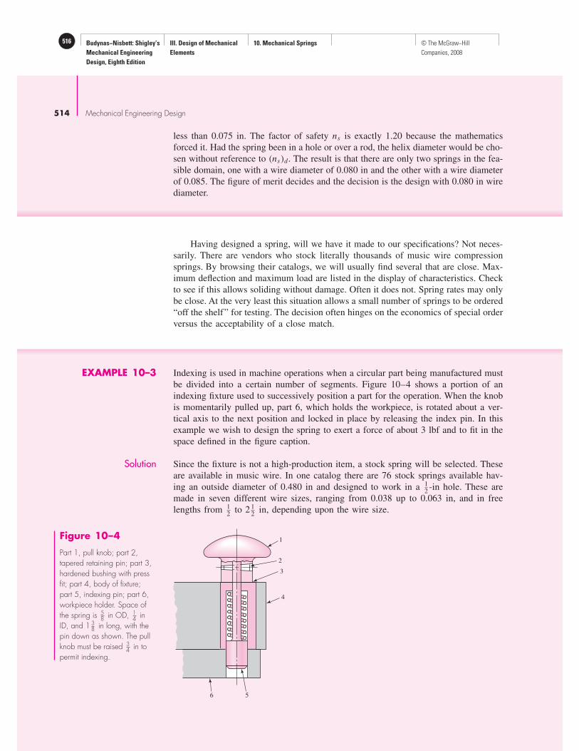
EXAMPLE 10–3 Indexing is used in machine operations when a circular part being manufactured must
be divided into a certain number of segments. Figure 10–4 shows a portion of an
indexing fixture used to successively position a part for the operation. When the knob
is momentarily pulled up, part 6, which holds the workpiece, is rotated about a ver-
tical axis to the next position and locked in place by releasing the index pin. In this
example we wish to design the spring to exert a force of about 3 lbf and to fit in the
space defined in the figure caption.
Solution Since the fixture is not a high-production item, a stock spring will be selected. These
are available in music wire. In one catalog there are 76 stock springs available hav-
ing an outside diameter of 0.480 in and designed to work in a 12-in hole. These are
made in seven different wire sizes, ranging from 0.038 up to 0.063 in, and in free
lengths from 12
to 2 12
in, depending upon the wire size.
6 5
4
3
2
1
+
Figure 10–4
Part 1, pull knob; part 2,tapered retaining pin; part 3,hardened bushing with pressfit; part 4, body of fixture;part 5, indexing pin; part 6,workpiece holder. Space ofthe spring is 5
8 in OD, 14 in
ID, and 1 38 in long, with the
pin down as shown. The pullknob must be raised 3
4 in topermit indexing.
Budynas−Nisbett: Shigley’s
Mechanical Engineering
Design, Eighth Edition
III. Design of Mechanical
Elements
10. Mechanical Springs 517© The McGraw−Hill
Companies, 2008
Mechanical Springs 515
Since the pull knob must be raised 34
in for indexing and the space for the spring is
1 38
in long when the pin is down, the solid length cannot be more than 58
in.
Let us begin by selecting a spring having an outside diameter of 0.480 in, a wire
size of 0.051 in, a free length of 1 34
in, 11 12
total turns, and plain ends. Then
m = 0.145 and A = 201 kpsi · inm for music wire. Then
Ssy = 0.45A
dm= 0.45
201
0.0510.145= 139.3 kpsi
With plain ends, from Table 10–1, the number of active turns is
Na = Nt = 11.5 turns
The mean coil diameter is D = OD − d = 0.480 − 0.051 = 0.429 in. From Eq. (10–9)
the spring rate is, for G = 11.85(106) psi from Table 10–5,
k = d4G
8D3 Na
= 0.0514(11.85)106
8(0.429)311.5= 11.0 lbf/in
From Table 10–1, the solid height Ls is
Ls = d(Nt + 1) = 0.051(11.5 + 1) = 0.638 in
The spring force when the pin is down, Fmin, is
Fmin = kymin = 11.0(1.75 − 1.375) = 4.13 lbf
When the spring is compressed solid, the spring force Fs is
Fs = kys = k(L0 − Ls) = 11.0(1.75 − 0.638) = 12.2 lbf
Since the spring index is C = D/d = 0.429/0.051 = 8.41,
K B = 4C + 2
4C − 3= 4(8.41) + 2
4(8.41) − 3= 1.163
and for the as-wound spring, the shear stress when compressed solid is
τs = K B
8Fs D
πd3= 1.163
8(12.2)0.429
π(0.051)3= 116 850 psi
The factor of safety when the spring is compressed solid is
ns = Ssy
τs
= 139.3
116.9= 1.19
Since ns is marginally adequate and Ls is larger than 58
in, we must investigate other
springs with a smaller wire size. After several investigations another spring has
possibilities. It is as-wound music wire, d = 0.045 in, 20 gauge (see Table A–25)
OD = 0.480 in, Nt = 11.5 turns, L0 = 1.75 in. Ssy is still 139.3 kpsi, and
D = OD − d = 0.480 − 0.045 = 0.435 in
Na = Nt = 11.5 turns
k = 0.0454(11.85)106
8(0.435)311.5= 6.42 lbf/in
Ls = d(Nt + 1) = 0.045(11.5 + 1) = 0.563 in
Budynas−Nisbett: Shigley’s
Mechanical Engineering
Design, Eighth Edition
III. Design of Mechanical
Elements
10. Mechanical Springs518 © The McGraw−Hill
Companies, 2008
516 Mechanical Engineering Design
Fmin = kymin = 6.42(1.75 − 1.375) = 2.41 lbf
Fs = 6.42(1.75 − 0.563) = 7.62 lbf
C = D
d= 0.435
0.045= 9.67
K B = 4(9.67) + 2
4(9.67) − 3= 1.140
τs = 1.1408(7.62)0.435
π(0.045)3= 105 600 psi
ns = Ssy
τs
= 139.3
105.6= 1.32
Now ns > 1.2, buckling is not possible as the coils are guarded by the hole surface,
and the solid length is less than 58
in, so this spring is selected. By using a stock
spring, we take advantage of economy of scale.
10–8 Critical Frequency of Helical SpringsIf a wave is created by a disturbance at one end of a swimming pool, this wave will
travel down the length of the pool, be reflected back at the far end, and continue in
this back-and-forth motion until it is finally damped out. The same effect occurs in
helical springs, and it is called spring surge. If one end of a compression spring is held
against a flat surface and the other end is disturbed, a compression wave is created that
travels back and forth from one end to the other exactly like the swimming-pool wave.
Spring manufacturers have taken slow-motion movies of automotive valve-spring
surge. These pictures show a very violent surging, with the spring actually jumping
out of contact with the end plates. Figure 10–5 is a photograph of a failure caused by
such surging.
When helical springs are used in applications requiring a rapid reciprocating
motion, the designer must be certain that the physical dimensions of the spring are not
such as to create a natural vibratory frequency close to the frequency of the applied force;
otherwise, resonance may occur, resulting in damaging stresses, since the internal
damping of spring materials is quite low.
The governing equation for the translational vibration of a spring is the wave
equation
∂2u
∂x2= W
kgl2
∂2u
∂t2(10–24)
where k = spring rate
g = acceleration due to gravity
l = length of spring
W = weight of spring
x = coordinate along length of spring
u = motion of any particle at distance x

Budynas−Nisbett: Shigley’s
Mechanical Engineering
Design, Eighth Edition
III. Design of Mechanical
Elements
10. Mechanical Springs 519© The McGraw−Hill
Companies, 2008
Mechanical Springs 517
9J. C. Wolford and G. M. Smith, “Surge of Helical Springs,” Mech. Eng. News, vol. 13, no. 1,
February 1976, pp. 4–9.
The solution to this equation is harmonic and depends on the given physical prop-
erties as well as the end conditions of the spring. The harmonic, natural, frequencies
for a spring placed between two flat and parallel plates, in radians per second, are
ω = mπ
√
kg
Wm = 1, 2, 3, . . .
where the fundamental frequency is found for m = 1, the second harmonic for m = 2,
and so on. We are usually interested in the frequency in cycles per second; since ω =2π f , we have, for the fundamental frequency in hertz,
f = 1
2
√
kg
W(10–25)
assuming the spring ends are always in contact with the plates.
Wolford and Smith9 show that the frequency is
f = 1
4
√
kg
W(10–26)
where the spring has one end against a flat plate and the other end free. They also
point out that Eq. (10–25) applies when one end is against a flat plate and the other
end is driven with a sine-wave motion.
The weight of the active part of a helical spring is
W = ALγ = πd2
4(π DNa)(γ ) = π2d2 DNaγ
4(10–27)
where γ is the specific weight.
Figure 10–5
Valve-spring failure in anoverrevved engine. Fractureis along the 45◦ line ofmaximum principal stressassociated with pure torsionalloading.
Budynas−Nisbett: Shigley’s
Mechanical Engineering
Design, Eighth Edition
III. Design of Mechanical
Elements
10. Mechanical Springs520 © The McGraw−Hill
Companies, 2008
518 Mechanical Engineering Design
The fundamental critical frequency should be greater than 15 to 20 times the fre-
quency of the force or motion of the spring in order to avoid resonance with the har-
monics. If the frequency is not high enough, the spring should be redesigned to
increase k or decrease W.
10–9 Fatigue Loading of Helical Compression SpringsSprings are almost always subject to fatigue loading. In many instances the number of
cycles of required life may be small, say, several thousand for a padlock spring or a
toggle-switch spring. But the valve spring of an automotive engine must sustain mil-
lions of cycles of operation without failure; so it must be designed for infinite life.
To improve the fatigue strength of dynamically loaded springs, shot peening can
be used. It can increase the torsional fatigue strength by 20 percent or more. Shot size
is about 164
in, so spring coil wire diameter and pitch must allow for complete cov-
erage of the spring surface.
The best data on the torsional endurance limits of spring steels are those reported by
Zimmerli.10 He discovered the surprising fact that size, material, and tensile strength have
no effect on the endurance limits (infinite life only) of spring steels in sizes under 38
in
(10 mm). We have already observed that endurance limits tend to level out at high ten-
sile strengths (Fig. 6–17), p. 275, but the reason for this is not clear. Zimmerli suggests
that it may be because the original surfaces are alike or because plastic flow during test-
ing makes them the same. Unpeened springs were tested from a minimum torsional stress
of 20 kpsi to a maximum of 90 kpsi and peened springs in the range 20 kpsi to 135 kpsi.
The corresponding endurance strength components for infinite life were found to be
Unpeened:
Ssa = 35 kpsi (241 MPa) Ssm = 55 kpsi (379 MPa) (10–28)
Peened:
Ssa = 57.5 kpsi (398 MPa) Ssm = 77.5 kpsi (534 MPa) (10–29)
For example, given an unpeened spring with Ssu = 211.5 kpsi, the Gerber ordinate inter-
cept for shear, from Eq. (6–42), p. 298, is
Sse = Ssa
1 −(
Ssm
Ssu
)2= 35
1 −(
55
211.5
)2= 37.5 kpsi
For the Goodman failure criterion, the intercept would be 47.3 kpsi. Each possible
wire size would change these numbers, since Ssu would change.
An extended study11 of available literature regarding torsional fatigue found that
for polished, notch-free, cylindrical specimens subjected to torsional shear stress, the
maximum alternating stress that may be imposed without causing failure is constant
and independent of the mean stress in the cycle provided that the maximum stress
range does not equal or exceed the torsional yield strength of the metal. With notches
and abrupt section changes this consistency is not found. Springs are free of notches
and surfaces are often very smooth. This failure criterion is known as the Sines failure
criterion in torsional fatigue.
10F. P. Zimmerli, “Human Failures in Spring Applications,” The Mainspring, no. 17, Associated Spring
Corporation, Bristol, Conn., August–September 1957.
11Oscar J. Horger (ed.), Metals Engineering: Design Handbook, McGraw-Hill, New York, 1953, p. 84.

Budynas−Nisbett: Shigley’s
Mechanical Engineering
Design, Eighth Edition
III. Design of Mechanical
Elements
10. Mechanical Springs 521© The McGraw−Hill
Companies, 2008
Mechanical Springs 519
In constructing certain failure criteria on the designers’ torsional fatigue diagram,
the torsional modulus of rupture Ssu is needed. We shall continue to employ Eq. (6–54),
p. 309, which is
Ssu = 0.67Sut (10–30)
In the case of shafts and many other machine members, fatigue loading in the form
of completely reversed stresses is quite ordinary. Helical springs, on the other hand,
are never used as both compression and extension springs. In fact, they are usually
assembled with a preload so that the working load is additional. Thus the stress-time
diagram of Fig. 6–23d, p. 293, expresses the usual condition for helical springs. The
worst condition, then, would occur when there is no preload, that is, when τmin = 0.
Now, we define
Fa = Fmax − Fmin
2(10–31a)
Fm = Fmax + Fmin
2(10–31b)
where the subscripts have the same meaning as those of Fig. 7–23d when applied to
the axial spring force F. Then the shear stress amplitude is
τa = K B
8Fa D
πd3(10–32)
where K B is the Bergsträsser factor, obtained from Eq. (10–6), and corrects for both
direct shear and the curvature effect. As noted in Sec. 10–2, the Wahl factor KW can
be used instead, if desired.
The midrange shear stress is given by the equation
τm = K B
8Fm D
πd3(10–33)
EXAMPLE 10–4 An as-wound helical compression spring, made of music wire, has a wire size of 0.092
in, an outside coil diameter of 916
in, a free length of 4 38
in, 21 active coils, and both ends
squared and ground. The spring is unpeened. This spring is to be assembled with a
preload of 5 lbf and will operate with a maximum load of 35 lbf during use.
(a) Estimate the factor of safety guarding against fatigue failure using a torsional
Gerber fatigue failure criterion with Zimmerli data.
(b) Repeat part (a) using the Sines torsional fatigue criterion (steady stress compo-
nent has no effect), with Zimmerli data.
(c) Repeat using a torsional Goodman failure criterion with Zimmerli data.
(d) Estimate the critical frequency of the spring.
Solution The mean coil diameter is D = 0.5625 − 0.092 = 0.4705 in. The spring index is C =D/d = 0.4705/0.092 = 5.11. Then
K B = 4C + 2
4C − 3= 4(5.11) + 2
4(5.11) − 3= 1.287

Budynas−Nisbett: Shigley’s
Mechanical Engineering
Design, Eighth Edition
III. Design of Mechanical
Elements
10. Mechanical Springs522 © The McGraw−Hill
Companies, 2008
520 Mechanical Engineering Design
From Eqs. (10–31),
Fa = 35 − 5
2= 15 lbf Fm = 35 + 5
2= 20 lbf
The alternating shear-stress component is found from Eq. (10–32) to be
τa = K B
8Fa D
πd3= (1.287)
8(15)0.4705
π(0.092)3(10−3) = 29.7 kpsi
Equation (10–33) gives the midrange shear-stress component
τm = K B
8Fm D
πd3= 1.287
8(20)0.4705
π(0.092)3(10−3) = 39.6 kpsi
From Table 10–4 we find A = 201 kpsi · inm and m = 0.145. The ultimate tensile
strength is estimated from Eq. (10–14) as
Sut = A
dm= 201
0.0920.145= 284.1 kpsi
Also the shearing ultimate strength is estimated from
Ssu = 0.67Sut = 0.67(284.1) = 190.3 kpsi
The load-line slope r = τa/τm = 29.7/39.6 = 0.75.
(a) The Gerber ordinate intercept for the Zimmerli data, Eq. (10–28), is
Sse = Ssa
1 − (Ssm/Ssu)2= 35
1 − (55/190.3)2= 38.2 kpsi
The amplitude component of strength Ssa , from Table 6–7, p. 299, is
Ssa = r2S2su
2Sse
−1 +
√
1 +(
2Sse
r Ssu
)2
= 0.752190.32
2(38.2)
−1 +
√
1 +[
2(38.2)
0.75(190.3)
]2
= 35.8 kpsi
and the fatigue factor of safety n f is given by
Answer n f = Ssa
τa
= 35.8
29.7= 1.21
(b) The Sines failure criterion ignores Ssm so that, for the Zimmerli data with Ssa =35 kpsi,
Answer n f = Ssa
τa
= 35
29.7= 1.18
(c) The ordinate intercept Sse for the Goodman failure criterion with the Zimmerli
data is
Sse = Ssa
1 − (Ssm/Ssu)= 35
1 − (55/190.3)= 49.2 kpsi

Budynas−Nisbett: Shigley’s
Mechanical Engineering
Design, Eighth Edition
III. Design of Mechanical
Elements
10. Mechanical Springs 523© The McGraw−Hill
Companies, 2008
Mechanical Springs 521
The amplitude component of the strength Ssa for the Goodman criterion, from
Table 6–6, p. 299, is
Ssa = r Sse Ssu
r Ssu + Sse
= 0.75(49.2)190.3
0.75(190.3) + 49.2= 36.6 kpsi
The fatigue factor of safety is given by
Answer n f = Ssa
τa
= 36.6
29.7= 1.23
(d ) Using Eq. (10–9) and Table 10–5, we estimate the spring rate as
k = d4G
8D3 Na
= 0.0924[11.75(106)]
8(0.4705)321= 48.1 lbf/in
From Eq. (10–27) we estimate the spring weight as
W = π2(0.0922)0.4705(21)0.284
4= 0.0586 lbf
and from Eq. (10–25) the frequency of the fundamental wave is
Answer fn = 1
2
[
48.1(386)
0.0586
]1/2
= 281 Hz
If the operating or exciting frequency is more than 281/20 = 14.1 Hz, the spring may
have to be redesigned.
We used three approaches to estimate the fatigue factor of safety in Ex. 10–5.
The results, in order of smallest to largest, were 1.18 (Sines), 1.21 (Gerber), and 1.23
(Goodman). Although the results were very close to one another, using the Zimmerli
data as we have, the Sines criterion will always be the most conservative and the
Goodman the least. If we perform a fatigue analysis using strength properties as was
done in Chap. 6, different results would be obtained, but here the Goodman criterion
would be more conservative than the Gerber criterion. Be prepared to see designers
or design software using any one of these techniques. This is why we cover them.
Which criterion is correct? Remember, we are performing estimates and only testing
will reveal the truth—statistically.
10–10 Helical Compression Spring Designfor Fatigue LoadingLet us begin with the statement of a problem. In order to compare a static spring to
a dynamic spring, we shall design the spring in Ex. 10–2 for dynamic service.
EXAMPLE 10–5 A music wire helical compression spring with infinite life is needed to resist a
dynamic load that varies from 5 to 20 lbf at 5 Hz while the end deflection varies from12
to 2 in. Because of assembly considerations, the solid height cannot exceed 1 in
and the free length cannot be more than 4 in. The springmaker has the following wire
sizes in stock: 0.069, 0.071, 0.080, 0.085, 0.090, 0.095, 0.105, and 0.112 in.
Budynas−Nisbett: Shigley’s
Mechanical Engineering
Design, Eighth Edition
III. Design of Mechanical
Elements
10. Mechanical Springs524 © The McGraw−Hill
Companies, 2008
522 Mechanical Engineering Design
Solution The a priori decisions are:
• Material and condition: for music wire, A = 201 kpsi · inm , m = 0.145, G =11.75(106) psi; relative cost is 2.6
• Surface treatment: unpeened
• End treatment: squared and ground
• Robust linearity: ξ = 0.15
• Set: use in as-wound condition
• Fatigue-safe: n f = 1.5 using the Sines-Zimmerli fatigue-failure criterion
• Function: Fmin = 5 lbf, Fmax = 20 lbf, ymin = 0.5 in, ymax = 2 in, spring operates
free (no rod or hole)
• Decision variable: wire size d
The figure of merit will be the volume of wire to wind the spring, Eq. (10–22). The
design strategy will be to set wire size d, build a table, inspect the table, and choose
the satisfactory spring with the highest figure of merit.
Solution Set d = 0.112 in. Then
Fa = 20 − 5
2= 7.5 lbf Fm = 20 + 5
2= 12.5 lbf
k = Fmax
ymax
= 20
2= 10 lbf/in
Sut = 201
0.1120.145= 276.1 kpsi
Ssu = 0.67(276.1) = 185.0 kpsi
Ssy = 0.45(276.1) = 124.2 kpsi
From Eq. (10–28), with the Sines criterion, Sse = Ssa = 35 kpsi. Equation (10–23)
can be used to determine C with Sse , n f , and Fa in place of Ssy , ns , and (1 + ξ )Fmax,
respectively. Thus,
α = Sse
n f
= 35 000
1.5= 23 333 psi
β = 8Fa
πd2= 8(7.5)
π(0.1122)= 1522.5 psi
C = 2(23 333) − 1522.5
4(1522.5)+
√
[
2(23 333) − 1522.5
4(1522.5)
]2
− 3(23 333)
4(1522.5)= 14.005
D = Cd = 14.005(0.112) = 1.569 in
Fs = (1 + ξ)Fmax = (1 + 0.15)20 = 23 lbf

Budynas−Nisbett: Shigley’s
Mechanical Engineering
Design, Eighth Edition
III. Design of Mechanical
Elements
10. Mechanical Springs 525© The McGraw−Hill
Companies, 2008
Mechanical Springs 523
Na = d4G
8D3k= 0.1124(11.75)(106)
8(1.569)310= 5.98 turns
Nt = Na + 2 = 5.98 + 2 = 7.98 turns
Ls = d Nt = 0.112(7.98) = 0.894 in
L0 = Ls + Fs
k= 0.894 + 23
10= 3.194 in
ID = 1.569 − 0.112 = 1.457 in
OD = 1.569 + 0.112 = 1.681 in
ys = L0 − Ls = 3.194 − 0.894 = 2.30 in
(L0)cr <2.63D
α= 2.63
(1.569)
0.5= 8.253 in
K B = 4(14.005) + 2
4(14.005) − 3= 1.094
W = π2d2 DNaγ
4= π20.1122(1.569)5.98(0.284)
4= 0.0825 lbf
fn = 0.5
√
386k
W= 0.5
√
386(10)
0.0825= 108 Hz
τa = K B
8Fa D
πd3= 1.094
8(7.5)1.569
π0.1123= 23 334 psi
τm = τa
Fm
Fa
= 23 33412.5
7.5= 38 890 psi
τs = τa
Fs
Fa
= 23 33423
7.5= 71 560 psi
n f = Ssa
τa
= 35 000
23 334= 1.5
ns = Ssy
τs
= 124 200
71 560= 1.74
fom = −(relative material cost)π2d2 Nt D/4
= −2.6π2(0.1122)(7.98)1.569/4 = −1.01
Inspection of the results shows that all conditions are satisfied except for 4 ≤ C ≤ 12.
Repeat the process using the other available wire sizes and develop the following

Budynas−Nisbett: Shigley’s
Mechanical Engineering
Design, Eighth Edition
III. Design of Mechanical
Elements
10. Mechanical Springs526 © The McGraw−Hill
Companies, 2008
524 Mechanical Engineering Design
table:
The problem-specific inequality constraints are
Ls ≤ 1 in
L0 ≤ 4 in
fn ≥ 5(20) = 100 Hz
The general constraints are
3 ≤ Na ≤ 15
4 ≤ C ≤ 12
(L0)cr > L0
We see that none of the diameters satisfy the given constraints. The 0.105-in-diameter
wire is the closest to satisfying all requirements. The value of C � 12.14 is not a
serious deviation and can be tolerated. However, the tight constraint on Ls needs to be
addressed. If the assembly conditions can be relaxed to accept a solid height of 1.116
in, we have a solution. If not, the only other possibility is to use the 0.112-in diameter
and accept a value C � 14, individually package the springs, and possibly reconsider
supporting the spring in service.
10–11 Extension SpringsExtension springs differ from compression springs in that they carry tensile loading,
they require some means of transferring the load from the support to the body of the
spring, and the spring body is wound with an initial tension. The load transfer can be
done with a threaded plug or a swivel hook; both of these add to the cost of the fin-
ished product, and so one of the methods shown in Fig. 10–6 is usually employed.
Stresses in the body of the extension spring are handled the same as compres-
sion springs. In designing a spring with a hook end, bending and torsion in the hook
d: 0.069 0.071 0.080 0.085 0.090 0.095 0.105 0.112
D 0.297 0.332 0.512 0.632 0.767 0.919 1.274 1.569
ID 0.228 0.261 0.432 0.547 0.677 0.824 1.169 1.457
OD 0.366 0.403 0.592 0.717 0.857 1.014 1.379 1.681
C 4.33 4.67 6.40 7.44 8.53 9.67 12.14 14.00
Na 127.2 102.4 44.8 30.5 21.3 15.4 8.63 6.0
Ls 8.916 7.414 3.740 2.750 2.100 1.655 1.116 0.895
L0 11.216 9.714 6.040 5.050 4.400 3.955 3.416 3.195
(L0)cr 1.562 1.744 2.964 3.325 4.036 4.833 6.703 8.250
nf 1.50 1.50 1.50 1.50 1.50 1.50 1.50 1.50
ns 1.86 1.85 1.82 1.81 1.79 1.78 1.75 1.74
fn 87.5 89.7 96.9 99.7 101.9 103.8 106.6 108
fom −1.17 −1.12 −0.983 −0.948 −0.930 −0.927 −0.958 −1.01

Budynas−Nisbett: Shigley’s
Mechanical Engineering
Design, Eighth Edition
III. Design of Mechanical
Elements
10. Mechanical Springs 527© The McGraw−Hill
Companies, 2008
Mechanical Springs 525
Figure 10–7
Ends for extension springs.(a) Usual design; stress at A isdue to combined axial forceand bending moment. (b) Sideview of part a; stress is mostlytorsion at B. (c) Improveddesign; stress at A is due tocombined axial force andbending moment. (d ) Sideview of part c ; stress at B ismostly torsion.
FF
A
A
(c) (d )
B
d
(a) (b)
r1
F F
B
d
r1
r2
r2
d
Note: Radius r1 is in the plane of
the end coil for curved beam
bending stress. Radius r2 is
at a right angle to the end
coil for torsional shear stress.
Figure 10–6
Types of ends used onextension springs. (Courtesy ofAssociated Spring.)
(a) Machine half loop–open (b) Raised hook
(c) Short twisted loop (d ) Full twisted loop
+ +
++
must be included in the analysis. In Fig. 10–7a and b a commonly used method of
designing the end is shown. The maximum tensile stress at A, due to bending and
axial loading, is given by
σA = F
[
(K )A
16D
πd3+ 4
πd2
]
(10–34)

Budynas−Nisbett: Shigley’s
Mechanical Engineering
Design, Eighth Edition
III. Design of Mechanical
Elements
10. Mechanical Springs528 © The McGraw−Hill
Companies, 2008
526 Mechanical Engineering Design
where (K )A is a bending stress correction factor for curvature, given by
(K )A = 4C21 − C1 − 1
4C1(C1 − 1)C1 = 2r1
d(10–35)
The maximum torsional stress at point B is given by
τB = (K )B
8F D
πd3(10–36)
where the stress correction factor for curvature, (K)B, is
(K )B = 4C2 − 1
4C2 − 4C2 = 2r2
d(10–37)
Figure 10–7c and d show an improved design due to a reduced coil diameter.
When extension springs are made with coils in contact with one another, they are
said to be close-wound. Spring manufacturers prefer some initial tension in close-wound
springs in order to hold the free length more accurately. The corresponding load-
deflection curve is shown in Fig. 10–8a, where y is the extension beyond the free length
4 6 8 10 12 14 16
5
10
15
20
25
30
35
40
25
50
75
100
125
150
175
200
225
250
275
300
Difficult
to control
Preferred
range
Available upon
special request
from springmaker
Difficult
to attain
Index
Tors
ional
str
ess
(unco
rrec
ted)
cause
d b
y i
nit
ial
tensi
on M
Pa
Tors
ional
str
ess
(unco
rrec
ted)
cause
d b
y i
nit
ial
tensi
on (
10
3psi
)
(c)
− +
Outside
diameter
Free length
Length of
bodyGap
Wire
diameter
Hook
length
Loop
length
Inside
diameter
Mean
diameter
(b)
F
y
F
Fi
y
(a)
Figure 10–8
(a) Geometry of the force Fand extension y curve of anextension spring; (b) geometryof the extension spring; and (c) torsional stresses due toinitial tension as a function ofspring index C in helicalextension springs.

Budynas−Nisbett: Shigley’s
Mechanical Engineering
Design, Eighth Edition
III. Design of Mechanical
Elements
10. Mechanical Springs 529© The McGraw−Hill
Companies, 2008
Mechanical Springs 527
Table 10–7
Maximum Allowable
Stresses (KW or KB
corrected) for Helical
Extension Springs in
Static Applications
Source: From DesignHandbook, 1987, p. 52.Courtesy of AssociatedSpring.
Percent of Tensile Strength
In Torsion In Bending
Materials Body End End
Patented, cold-drawn or 45–50 40 75hardened and temperedcarbon and low-alloysteels
Austenitic stainless 35 30 55steel and nonferrousalloys
This information is based on the following conditions: set not removed and low temperature heattreatment applied. For springs that require high initial tension, use the same percent of tensilestrength as for end.
L0 and Fi is the initial tension in the spring that must be exceeded before the spring
deflects. The load-deflection relation is then
F = Fi + ky (10–38)
where k is the spring rate. The free length L0 of a spring measured inside the end
loops or hooks as shown in Fig. 10–8b can be expressed as
L0 = 2(D − d) + (Nb + 1)d = (2C − 1 + Nb)d (10–39)
where D is the mean coil diameter, Nb is the number of body coils, and C is the
spring index. With ordinary twisted end loops as shown in Fig. 10–8b, to account for
the deflection of the loops in determining the spring rate k, the equivalent number of
active helical turns Na for use in Eq. (10–9) is
Na = Nb + G
E(10–40)
where G and E are the shear and tensile moduli of elasticity, respectively (see Prob.
10–31).
The initial tension in an extension spring is created in the winding process by
twisting the wire as it is wound onto the mandrel. When the spring is completed and
removed from the mandrel, the initial tension is locked in because the spring cannot
get any shorter. The amount of initial tension that a springmaker can routinely incor-
porate is as shown in Fig. 10–8c. The preferred range can be expressed in terms of
the uncorrected torsional stress τi as
τi = 33 500
exp(0.105C)± 1000
(
4 − C − 3
6.5
)
psi (10–41)
where C is the spring index.
Guidelines for the maximum allowable corrected stresses for static applications of
extension springs are given in Table 10–7.
Budynas−Nisbett: Shigley’s
Mechanical Engineering
Design, Eighth Edition
III. Design of Mechanical
Elements
10. Mechanical Springs530 © The McGraw−Hill
Companies, 2008
528 Mechanical Engineering Design
EXAMPLE 10–6 A hard-drawn steel wire extension spring has a wire diameter of 0.035 in, an outside
coil diameter of 0.248 in, hook radii of r1 = 0.106 in and r2 = 0.089 in, and an initial
tension of 1.19 lbf. The number of body turns is 12.17. From the given information:
(a) Determine the physical parameters of the spring.
(b) Check the initial preload stress conditions.
(c) Find the factors of safety under a static 5.25-lbf load.
Solution (a) D = OD − d = 0.248 − 0.035 = 0.213 in
C = D
d= 0.213
0.035= 6.086
K B = 4C + 2
4C − 3= 1.234
Eq. (10–40): Na = Nb + G/E = 12.17 + 11.5/28.7 = 12.57 turns
Eq. (10–9): k = d4G
8D3 Na
= 0.0354(11.5)106
8(0.2133)12.57= 17.76 lbf/in
Eq. (10–39): L0 = (2C − 1 + Nb)d = [2(6.086) − 1 + 12.17] 0.035 = 0.817 in
The deflection under the service load is
ymax = Fmax − Fi
k= 5.25 − 1.19
17.76= 0.229 in
where the spring length becomes L = L0 + y = 0.817 + 0.229 = 1.046 in.
(b) The uncorrected initial stress is given by Eq. (10–3) without the correction factor.
That is,
(τi )uncorr = 8Fi D
πd3= 8(1.19)0.213(10−3)
π(0.0353)= 15.1 kpsi
The preferred range is given by Eq. (10–41) and for this case is
(τi )pref = 33 500
exp(0.105C)± 1000
(
4 − C − 3
6.5
)
= 33 500
exp[0.105(6.086)]± 1000
(
4 − 6.086 − 3
6.5
)
= 17 681 ± 3525 = 21.2, 14.2 kpsi
Answer Thus, the initial tension of 15.1 kpsi is in the preferred range.
(c) For hard-drawn wire, Table 10–4 gives m = 0.190 and A = 140 kpsi · inm . From
Eq. (10–14)
Sut = A
dm= 140
0.0350.190= 264.7 kpsi
For torsional shear in the main body of the spring, from Table 10–7,
Ssy = 0.45Sut = 0.45(264.7) = 119.1 kpsi
Budynas−Nisbett: Shigley’s
Mechanical Engineering
Design, Eighth Edition
III. Design of Mechanical
Elements
10. Mechanical Springs 531© The McGraw−Hill
Companies, 2008
Mechanical Springs 529
The shear stress under the service load is
τmax = 8K B Fmax D
πd3= 8(1.234)5.25(0.213)
π(0.0353)(10−3) = 82.0 kpsi
Thus, the factor of safety is
Answer n = Ssy
τmax
= 119.1
82.0= 1.45
For the end-hook bending at A,
C1 = 2r1/d = 2(0.106)/0.0.035 = 6.057
From Eq. (10–35)
(K )A = 4C21 − C1 − 1
4C1(C1 − 1)= 4(6.0572) − 6.057 − 1
4(6.057)(6.057 − 1)= 1.14
From Eq. (10–34)
σA = Fmax
[
(K )A
16D
πd3+ 4
πd2
]
= 5.25
[
1.1416(0.213)
π(0.0353)+ 4
π(0.0352)
]
(10−3) = 156.9 kpsi
The yield strength, from Table 10–7, is given by
Sy = 0.75Sut = 0.75(264.7) = 198.5 kpsi
The factor of safety for end-hook bending at A is then
Answer n A = Sy
σA
= 198.5
156.9= 1.27
For the end-hook in torsion at B, from Eq. (10–37)
C2 = 2r2/d = 2(0.089)/0.035 = 5.086
(K )B = 4C2 − 1
4C2 − 4= 4(5.086) − 1
4(5.086) − 4= 1.18
and the corresponding stress, given by Eq. (10–36), is
τB = (K )B
8Fmax D
πd3= 1.18
8(5.25)0.213
π(0.0353)(10−3) = 78.4 kpsi
Using Table 10–7 for yield strength, the factor of safety for end-hook torsion at B is
Answer nB = (Ssy)B
τB
= 0.4(264.7)
78.4= 1.35
Yield due to bending of the end hook will occur first.
Next, let us consider a fatigue problem.
Budynas−Nisbett: Shigley’s
Mechanical Engineering
Design, Eighth Edition
III. Design of Mechanical
Elements
10. Mechanical Springs532 © The McGraw−Hill
Companies, 2008
530 Mechanical Engineering Design
EXAMPLE 10–7 The helical coil extension spring of Ex. 10–6 is subjected to a dynamic loading from
1.5 to 5 lbf. Estimate the factors of safety using the Gerber failure criterion for (a) coil
fatigue, (b) coil yielding, (c) end-hook bending fatigue at point A of Fig. 10–7a, and
(d) end-hook torsional fatigue at point B of Fig. 10–7b.
Solution A number of quantities are the same as in Ex. 10–6: d = 0.035 in, Sut = 264.7 kpsi,
D = 0.213 in, r1 = 0.106 in, C = 6.086, K B = 1.234, (K )A = 1.14, (K)B = 1.18,
Nb = 12.17 turns, L0 = 0.817 in, k = 17.76 lbf/in, Fi = 1.19 lbf, and (τi)uncorr = 15.1
kpsi. Then
Fa = (Fmax − Fmin)/2 = (5 − 1.5)/2 = 1.75 lbf
Fm = (Fmax + Fmin)/2 = (5 + 1.5)/2 = 3.25 lbf
The strengths from Ex. 10–6 include Sut = 264.7 kpsi, Sy = 198.5 kpsi, and Ssy =119.1 kpsi. The ultimate shear strength is estimated from Eq. (10–30) as
Ssu = 0.67Sut = 0.67(264.7) = 177.3 kpsi
(a) Body-coil fatigue:
τa = 8K B Fa D
πd3= 8(1.234)1.75(0.213)
π(0.0353)(10−3) = 27.3 kpsi
τm = Fm
Fa
τa = 3.25
1.7527.3 = 50.7 kpsi
Using the Zimmerli data of Eq. (10–28) gives
Sse = Ssa
1 −(
Ssm
Ssu
)2= 35
1 −(
55
177.3
)2= 38.7 kpsi
From Table 6–7, p. 299, the Gerber fatigue criterion for shear is
Answer (n f )body = 1
2
(
Ssu
τm
)2τa
Sse
−1 +
√
1 +(
2τm
Ssu
Sse
τa
)2
= 1
2
(
177.3
50.7
)227.3
38.7
−1 +
√
1 +(
250.7
177.3
38.7
27.3
)2
= 1.24
(b) The load-line for the coil body begins at Ssm = τi and has a slope r = τa/(τm − τi ).
It can be shown that the intersection with the yield line is given by (Ssa)y =[r/(r + 1)](Ssy − τi ). Consequently, τi = (Fi/Fa)τa = (1.19/1.75)27.3 = 18.6 kpsi,
r = 27.3/(50.7 − 18.6) = 0.850, and
(Ssa)y = 0.850
0.850 + 1(119.1 − 18.6) = 46.2 kpsi
Thus,
Answer (ny)body = (Ssa)y
τa
= 46.2
27.3= 1.69
Budynas−Nisbett: Shigley’s
Mechanical Engineering
Design, Eighth Edition
III. Design of Mechanical
Elements
10. Mechanical Springs 533© The McGraw−Hill
Companies, 2008
Mechanical Springs 531
(c) End-hook bending fatigue: using Eqs. (10–34) and (10–35) gives
σa = Fa
[
(K )A
16D
πd3+ 4
πd2
]
= 1.75
[
1.1416(0.213)
π(0.0353)+ 4
π(0.0352)
]
(10−3) = 52.3 kpsi
σm = Fm
Fa
σa = 3.25
1.7552.3 = 97.1 kpsi
To estimate the tensile endurance limit using the distortion-energy theory,
Se = Sse/0.577 = 38.7/0.577 = 67.1 kpsi
Using the Gerber criterion for tension gives
Answer (n f )A = 1
2
(
Sut
σm
)2σa
Se
−1 +
√
1 +(
2σm
Sut
Se
σa
)2
= 1
2
(
264.7
97.1
)252.3
67.1
−1 +
√
1 +(
297.1
264.7
67.1
52.3
)2
= 1.08
(d) End-hook torsional fatigue: from Eq. (10–36)
(τa)B = (K )B
8Fa D
πd3= 1.18
8(1.75)0.213
π(0.0353)(10−3) = 26.1 kpsi
(τm)B = Fm
Fa
(τa)B = 3.25
1.7526.1 = 48.5 kpsi
Then, again using the Gerber criterion, we obtain
Answer (n f )B = 1
2
(
Ssu
τm
)2τa
Sse
−1 +
√
1 +(
2τm
Ssu
Sse
τa
)2
= 1
2
(
177.3
48.5
)226.1
38.7
−1 +
√
1 +(
248.5
177.3
38.7
26.1
)2
= 1.30
The analyses in Exs. 10–6 and 10–7 show how extension springs differ from com-
pression springs. The end hooks are usually the weakest part, with bending usually
controlling. We should also appreciate that a fatigue failure separates the extension
spring under load. Flying fragments, lost load, and machine shutdown are threats to
personal safety as well as machine function. For these reasons higher design factors
are used in extension-spring design than in the design of compression springs.
In Ex. 10–7 we estimated the endurance limit for the hook in bending using the
Zimmerli data, which are based on torsion in compression springs and the distortion the-
ory. An alternative method is to use Table 10–8, which is based on a stress-ratio of R =τmin/τmax = 0. For this case, τa = τm = τmax/2. Label the strength values of Table 10–8

Budynas−Nisbett: Shigley’s
Mechanical Engineering
Design, Eighth Edition
III. Design of Mechanical
Elements
10. Mechanical Springs534 © The McGraw−Hill
Companies, 2008
532 Mechanical Engineering Design
Table 10–8
Maximum Allowable
Stresses for ASTM
A228 and Type 302
Stainless Steel Helical
Extension Springs in
Cyclic Applications
Source: From DesignHandbook, 1987, p. 52.Courtesy of AssociatedSpring.
Percent of Tensile Strength
Number In Torsion In Bending
of Cycles Body End End
105 36 34 51
106 33 30 47
107 30 28 45
This information is based on the following conditions: not shot-peened, no surging and ambientenvironment with a low temperature heat treatment applied. Stress ratio � 0.
as Sr for bending or Ssr for torsion. Then for torsion, for example, Ssa = Ssm = Ssr/2
and the Gerber ordinate intercept, given by Eq. (6–42) for shear, is
Sse = Ssa
1 − (Ssm/Ssu)2
= Ssr/2
1 −(
Ssr/2
Ssu
)2(10–42)
So in Ex. 10–7 an estimate for the bending endurance limit from Table 10–8 would be
Sr = 0.45Sut = 0.45(264.7) = 119.1 kpsi
and from Eq. (10–42)
Se = Sr/2
1 − [Sr/ (2Sut)]2
= 119.1/2
1 −(
119.1/2
264.7
)2= 62.7 kpsi
Using this in place of 67.1 kpsi in Ex. 10–7 results in (n f )A = 1.03, a reduction of
5 percent.
10–12 Helical Coil Torsion SpringsWhen a helical coil spring is subjected to end torsion, it is called a torsion spring. It
is usually close-wound, as is a helical coil extension spring, but with negligible initial
tension. There are single-bodied and double-bodied types as depicted in Fig. 10–9. As
shown in the figure, torsion springs have ends configured to apply torsion to the coil
body in a convenient manner, with short hook, hinged straight offset, straight torsion,
and special ends. The ends ultimately connect a force at a distance from the coil axis
to apply a torque. The most frequently encountered (and least expensive) end is the
straight torsion end. If intercoil friction is to be avoided completely, the spring can be
wound with a pitch that just separates the body coils. Helical coil torsion springs are
usually used with a rod or arbor for reactive support when ends cannot be built in, to
maintain alignment, and to provide buckling resistance if necessary.
The wire in a torsion spring is in bending, in contrast to the torsion encountered
in helical coil compression and extension springs. The springs are designed to wind
tighter in service. As the applied torque increases, the inside diameter of the coil
decreases. Care must be taken so that the coils do not interfere with the pin, rod, or
arbor. The bending mode in the coil might seem to invite square- or rectangular-cross-
section wire, but cost, range of materials, and availability discourage its use.

Budynas−Nisbett: Shigley’s
Mechanical Engineering
Design, Eighth Edition
III. Design of Mechanical
Elements
10. Mechanical Springs 535© The McGraw−Hill
Companies, 2008
Mechanical Springs 533
Torsion springs are familiar in clothespins, window shades, and animal traps,
where they may be seen around the house, and out of sight in counterbalance mech-
anisms, ratchets, and a variety of other machine components. There are many stock
springs that can be purchased off-the-shelf from a vendor. This selection can add
economy of scale to small projects, avoiding the cost of custom design and small-
run manufacture.
Describing the End Location
In specifying a torsion spring, the ends must be located relative to each other. Commer-
cial tolerances on these relative positions are listed in Table 10–9. The simplest scheme
for expressing the initial unloaded location of one end with respect to the other is in terms
of an angle β defining the partial turn present in the coil body as Np = β/360◦, as shown
in Fig. 10–10. For analysis purposes the nomenclature of Fig. 10–10 can be used. Com-
munication with a springmaker is often in terms of the back-angle α.
The number of body turns Nb is the number of turns in the free spring body by
count. The body-turn count is related to the initial position angle β by
Nb = integer + β
360◦ = integer + Np
Figure 10–9
Torsion springs. (Courtesy ofAssociated Spring.)
Short hook ends
Special ends
Double torsion
Hinge ends
Straight offset
Straight torsion
Table 10–9
End Position Tolerances
for Helical Coil Torsion
Springs (for D/d Ratios
up to and Including 16)
Source: From DesignHandbook, 1987, p. 52.Courtesy of AssociatedSpring.
Total Coils Tolerance: Degrees*
Up to 3 8
Over 3–10 10
Over 10–20 15
Over 20–30 20
Over 30 25
∗Closer tolerances available on request.

Budynas−Nisbett: Shigley’s
Mechanical Engineering
Design, Eighth Edition
III. Design of Mechanical
Elements
10. Mechanical Springs536 © The McGraw−Hill
Companies, 2008
534 Mechanical Engineering Design
where Np is the number of partial turns. The above equation means that Nb takes on
noninteger, discrete values such as 5.3, 6.3, 7.3, . . . , with successive differences of 1
as possibilities in designing a specific spring. This consideration will be discussed later.
Bending Stress
A torsion spring has bending induced in the coils, rather than torsion. This means that
residual stresses built in during winding are in the same direction but of opposite sign
to the working stresses that occur during use. The strain-strengthening locks in resid-
ual stresses opposing working stresses provided the load is always applied in the wind-
ing sense. Torsion springs can operate at bending stresses exceeding the yield strength
of the wire from which it was wound.
The bending stress can be obtained from curved-beam theory expressed in the form
σ = KMc
I
where K is a stress-correction factor. The value of K depends on the shape of the wire
cross section and whether the stress sought is at the inner or outer fiber. Wahl analytically
determined the values of K to be, for round wire,
Ki = 4C2 − C − 1
4C(C − 1)Ko = 4C2 + C − 1
4C(C + 1)(10–43)
where C is the spring index and the subscripts i and o refer to the inner and outer
fibers, respectively. In view of the fact that Ko is always less than unity, we shall use
Ki to estimate the stresses. When the bending moment is M = Fr and the section
modulus I/c = d3/32, we express the bending equation as
σ = Ki
32Fr
πd3(10–44)
which gives the bending stress for a round-wire torsion spring.
Deflection and Spring Rate
For torsion springs, angular deflection can be expressed in radians or revolutions
(turns). If a term contains revolution units the term will be expressed with a prime
sign. The spring rate k ′ is expressed in units of torque/revolution (lbf · in/rev or
N · mm/rev) and moment is proportional to angle θ ′ expressed in turns rather than
radians. The spring rate, if linear, can be expressed as
k ′ = M1
θ ′1
= M2
θ ′2
= M2 − M1
θ ′2 − θ ′
1
(10–45)
where the moment M can be expressed as Fl or Fr .
Figure 10–10
The free-end location angle isβ. The rotational coordinate θis proportional to the productFl. Its back angle is α. For allpositions of the moving endθ + α = � = constant.
�
F
l
Budynas−Nisbett: Shigley’s
Mechanical Engineering
Design, Eighth Edition
III. Design of Mechanical
Elements
10. Mechanical Springs 537© The McGraw−Hill
Companies, 2008
Mechanical Springs 535
The angle subtended by the end deflection of a cantilever, when viewed from the
built-in ends, is y/ l rad. From Table A–9–1,
θe = y
l= Fl2
3E I= Fl2
3E(πd4/64)= 64Ml
3πd4 E(10–46)
For a straight torsion end spring, end corrections such as Eq. (10–46) must be added
to the body-coil deflection. The strain energy in bending is, from Eq. (4–18),
U =∫
M2 dx
2E I
For a torsion spring, M = Fl = Fr , and integration must be accomplished over the
length of the body-coil wire. The force F will deflect through a distance rθ where θ is
the angular deflection of the coil body, in radians. Applying Castigliano’s theorem gives
rθ = ∂U
∂ F=∫ π DNb
0
∂
∂ F
(
F2r2 dx
2E I
)
=∫ π DNb
0
Fr2 dx
E I
Substituting I = πd4/64 for round wire and solving for θ gives
θ = 64Fr DNb
d4 E= 64M DNb
d4 E
The total angular deflection in radians is obtained by adding Eq. (10–46) for each end
of lengths l1, l2:
θt = 64M DNb
d4 E+ 64Ml1
3πd4 E+ 64Ml2
3πd4 E= 64M D
d4 E
(
Nb + l1 + l2
3π D
)
(10–47)
The equivalent number of active turns Na is expressed as
Na = Nb + l1 + l2
3π D(10–48)
The spring rate k in torque per radian is
k = Fr
θt
= M
θt
= d4 E
64DNa
(10–49)
The spring rate may also be expressed as torque per turn. The expression for this is
obtained by multiplying Eq. (10–49) by 2π rad/turn. Thus spring rate k ′ (units
torque/turn) is
k ′ = 2πd4 E
64DNa
= d4 E
10.2DNa
(10–50)
Tests show that the effect of friction between the coils and arbor is such that the con-
stant 10.2 should be increased to 10.8. The equation above becomes
k ′ = d4 E
10.8DNa
(10–51)
(units torque per turn). Equation (10–51) gives better results. Also Eq. (10–47) becomes
θ ′t = 10.8M D
d4 E
(
Nb + l1 + l2
3π D
)
(10–52)

Budynas−Nisbett: Shigley’s
Mechanical Engineering
Design, Eighth Edition
III. Design of Mechanical
Elements
10. Mechanical Springs538 © The McGraw−Hill
Companies, 2008
536 Mechanical Engineering Design
Torsion springs are frequently used over a round bar or pin. When the load is applied
to a torsion spring, the spring winds up, causing a decrease in the inside diameter of
the coil body. It is necessary to ensure that the inside diameter of the coil never
becomes equal to or less than the diameter of the pin, in which case loss of spring
function would ensue. The helix diameter of the coil D′ becomes
D′ = Nb D
Nb + θ ′c
(10–53)
where θ ′c is the angular deflection of the body of the coil in number of turns, given by
θ ′c = 10.8M DNb
d4 E(10–54)
The new inside diameter D′i = D′ − d makes the diametral clearance � between the
body coil and the pin of diameter Dp equal to
� = D′ − d − Dp = Nb D
Nb + θ ′c
− d − Dp (10–55)
Equation (10–55) solved for Nb is
Nb = θ ′c(� + d + Dp)
D − � − d − Dp
(10–56)
which gives the number of body turns corresponding to a specified diametral clear-
ance of the arbor. This angle may not be in agreement with the necessary partial-turn
remainder. Thus the diametral clearance may be exceeded but not equaled.
Static Strength
First column entries in Table 10–6 can be divided by 0.577 (from distortion-energy
theory) to give
Sy =
0.78Sut Music wire and cold-drawn carbon steels
0.87Sut OQ&T carbon and low-alloy steels
0.61Sut Austenitic stainless steel and nonferrous alloys
(10–57)
Fatigue Strength
Since the spring wire is in bending, the Sines equation is not applicable. The Sines
model is in the presence of pure torsion. Since Zimmerli’s results were for compres-
sion springs (wire in pure torsion), we will use the repeated bending stress (R = 0)
values provided by Associated Spring in Table 10–10. As in Eq. (10–40) we will use
the Gerber fatigue-failure criterion incorporating the Associated Spring R = 0 fatigue
strength Sr :
Se = Sr/2
1 −(
Sr/2
Sut
)2(10–58)
The value of Sr (and Se) has been corrected for size, surface condition, and type of
loading, but not for temperature or miscellaneous effects. The Gerber fatigue criterion
is now defined. The strength-amplitude component is given by Table 6–7, p. 299, as
Sa = r2S2ut
2Se
−1 +
√
1 +(
2Se
r Sut
)2
(10–59)
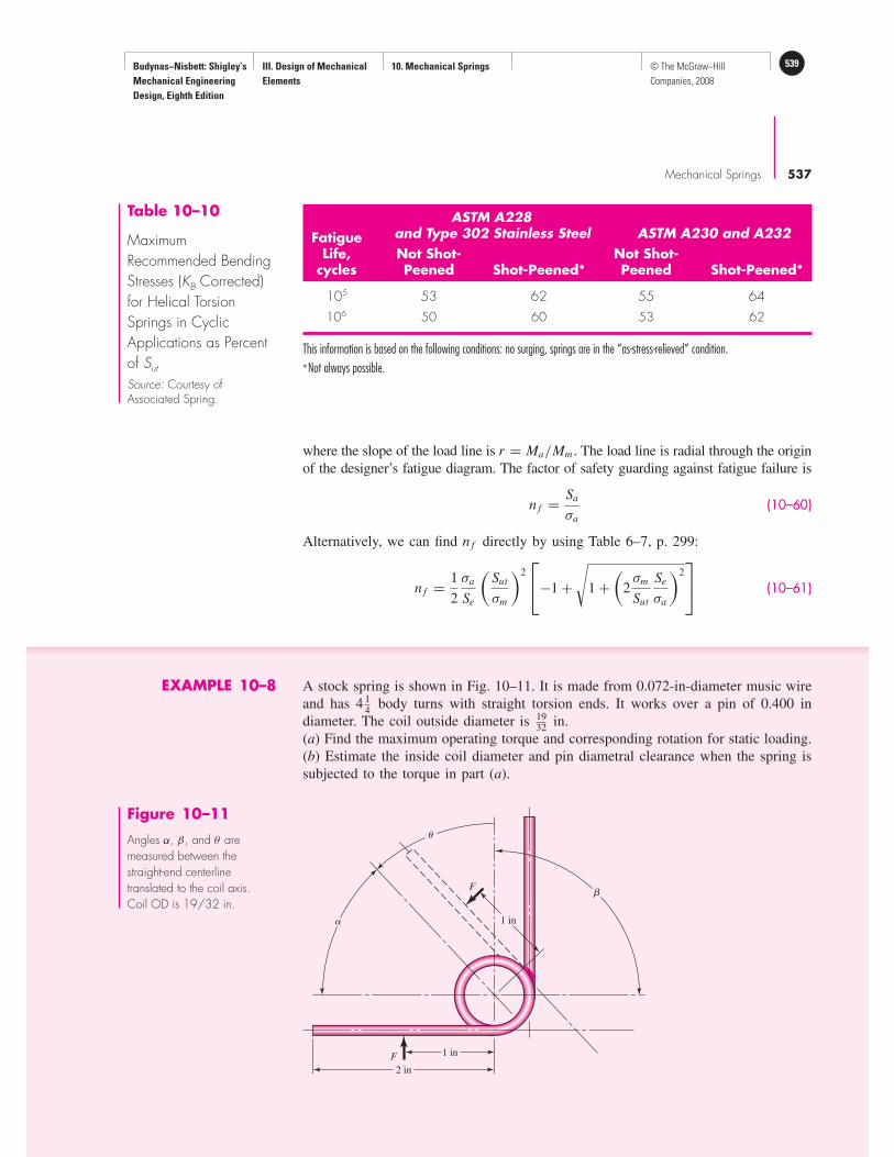
Budynas−Nisbett: Shigley’s
Mechanical Engineering
Design, Eighth Edition
III. Design of Mechanical
Elements
10. Mechanical Springs 539© The McGraw−Hill
Companies, 2008
Mechanical Springs 537
Figure 10–11
Angles α, β, and θ aremeasured between thestraight-end centerlinetranslated to the coil axis.Coil OD is 19/32 in.
F
F
2 in
1 in
1 in�
where the slope of the load line is r = Ma/Mm . The load line is radial through the origin
of the designer’s fatigue diagram. The factor of safety guarding against fatigue failure is
n f = Sa
σa
(10–60)
Alternatively, we can find n f directly by using Table 6–7, p. 299:
n f = 1
2
σa
Se
(
Sut
σm
)2
−1 +
√
1 +(
2σm
Sut
Se
σa
)2
(10–61)
EXAMPLE 10–8 A stock spring is shown in Fig. 10–11. It is made from 0.072-in-diameter music wire
and has 4 14
body turns with straight torsion ends. It works over a pin of 0.400 in
diameter. The coil outside diameter is 1932
in.
(a) Find the maximum operating torque and corresponding rotation for static loading.
(b) Estimate the inside coil diameter and pin diametral clearance when the spring is
subjected to the torque in part (a).
Table 10–10
Maximum
Recommended Bending
Stresses (KB Corrected)
for Helical Torsion
Springs in Cyclic
Applications as Percent
of Sut
Source: Courtesy ofAssociated Spring.
ASTM A228
Fatigue and Type 302 Stainless Steel ASTM A230 and A232
Life, Not Shot- Not Shot-cycles Peened Shot-Peened* Peened Shot-Peened*
105 53 62 55 64
106 50 60 53 62
This information is based on the following conditions: no surging, springs are in the “as-stress-relieved” condition. ∗Not always possible.

Budynas−Nisbett: Shigley’s
Mechanical Engineering
Design, Eighth Edition
III. Design of Mechanical
Elements
10. Mechanical Springs540 © The McGraw−Hill
Companies, 2008
538 Mechanical Engineering Design
(c) Estimate the fatigue factor of safety n f if the applied moment varies between
Mmin = 1 to Mmax = 5 lbf · in.
Solution (a) For music wire, from Table 10–4 we find that A = 201 kpsi · inm and m = 0.145.
Therefore,
Sut = A
dm= 201
(0.072)0.145= 294.4 kpsi
Using Eq. (10–57) gives
Sy = 0.78Sut = 0.78(294.4) = 229.6 kpsi
The mean coil diameter is D = 19/32 − 0.072 = 0.5218 in. The spring index C =D/d = 0.5218/0.072 = 7.247. The bending stress correction factor Ki from Eq. (10–43),
is
Ki = 4(7.247)2 − 7.247 − 1
4(7.247)(7.247 − 1)= 1.115
Now rearrange Eq. (10–44), substitute Sy for σ , and solve for the maximum torque
Fr to obtain
Mmax = (Fr)max = πd3Sy
32Ki
= π(0.072)3229 600
32(1.115)= 7.546 lbf · in
Note that no factor of safety has been used. Next, from Eq. (10–54), the number of
turns of the coil body θ ′c is
θ ′c = 10.8MDNb
d4 E= 10.8(7.546)0.5218(4.25)
0.0724(28.5)106= 0.236 turn
Answer (θ ′c)deg = 0.236(360◦) = 85.0◦
The active number of turns Na , from Eq. (10–48), is
Na = Nb + l1 + l2
3π D= 4.25 + 1 + 1
3π(0.5218)= 4.657 turns
The spring rate of the complete spring, from Eq. (10–51), is
k ′ = 0.0724(28.5)106
10.8(0.5218)4.657= 29.18 lbf · in/turn
The number of turns of the complete spring θ ′ is
θ ′ = M
k ′ = 7.546
29.18= 0.259 turn
Answer (θ ′s)deg = 0.259(360◦) = 93.24◦
(b) With no load, the mean coil diameter of the spring is 0.5218 in. From Eq. (10–53),
D′ = Nb D
Nb + θ ′c
= 4.25(0.5218)
4.25 + 0.236= 0.494 in
Budynas−Nisbett: Shigley’s
Mechanical Engineering
Design, Eighth Edition
III. Design of Mechanical
Elements
10. Mechanical Springs 541© The McGraw−Hill
Companies, 2008
Mechanical Springs 539
The diametral clearance between the inside of the spring coil and the pin at load is
Answer � = D′ − d − Dp = 0.494 − 0.072 − 0.400 = 0.022 in
(c) Fatigue:
Ma = (Mmax − Mmin)/2 = (5 − 1)/2 = 2 lbf · in
Mm = (Mmax + Mmin)/2 = (5 + 1)/2 = 3 lbf · in
r = Ma
Mm
= 2
3
σa = Ki
32Ma
πd3= 1.115
32(2)
π0.0723= 60 857 psi
σm = Mm
Ma
σa = 3
2(60 857) = 91 286 psi
From Table 10–10, Sr = 0.50Sut = 0.50(294.4) = 147.2 kpsi. Then
Se = 147.2/2
1 −(
147.2/2
294.4
)2= 78.51 kpsi
The amplitude component of the strength Sa , from Eq. (10–59), is
Sa = (2/3)2294.42
2(78.51)
−1 +
√
1 +(
2
2/3
78.51
294.4
)2
= 68.85 kpsi
The fatigue factor of safety is
Answer n f = Sa
σa
= 68.85
60.86= 1.13
10–13 Belleville SpringsThe inset of Fig. 10–12 shows a coned-disk spring, commonly called a Belleville
spring. Although the mathematical treatment is beyond the scope of this book, you
should at least become familiar with the remarkable characteristics of these springs.
Aside from the obvious advantage that a Belleville spring occupies only a small
space, variation in the h/t ratio will produce a wide variety of load-deflection curve
shapes, as illustrated in Fig. 10–12. For example, using an h/t ratio of 2.83 or larger
gives an S curve that might be useful for snap-acting mechanisms. A reduction of the
ratio to a value between 1.41 and 2.1 causes the central portion of the curve to become
horizontal, which means that the load is constant over a considerable deflection range.
A higher load for a given deflection may be obtained by nesting, that is, by stack-
ing the springs in parallel. On the other hand, stacking in series provides a larger
deflection for the same load, but in this case there is danger of instability.

Budynas−Nisbett: Shigley’s
Mechanical Engineering
Design, Eighth Edition
III. Design of Mechanical
Elements
10. Mechanical Springs542 © The McGraw−Hill
Companies, 2008
540 Mechanical Engineering Design
10–14 Miscellaneous SpringsThe extension spring shown in Fig. 10–13 is made of slightly curved strip steel, not
flat, so that the force required to uncoil it remains constant; thus it is called a constant-
force spring. This is equivalent to a zero spring rate. Such springs can also be man-
ufactured having either a positive or a negative spring rate.
A volute spring, shown in Fig. 10–14a, is a wide, thin strip, or “flat,” of mater-
ial wound on the flat so that the coils fit inside one another. Since the coils do not
stack, the solid height of the spring is the width of the strip. A variable-spring scale,
in a compression volute spring, is obtained by permitting the coils to contact the sup-
port. Thus, as the deflection increases, the number of active coils decreases. The volute
spring has another important advantage that cannot be obtained with round-wire
springs: if the coils are wound so as to contact or slide on one another during action,
the sliding friction will serve to damp out vibrations or other unwanted transient
disturbances.
A conical spring, as the name implies, is a coil spring wound in the shape of a
cone (see Prob. 10–22). Most conical springs are compression springs and are wound
with round wire. But a volute spring is a conical spring too. Probably the principal
advantage of this type of spring is that it can be wound so that the solid height is
only a single wire diameter.
Flat stock is used for a great variety of springs, such as clock springs, power
springs, torsion springs, cantilever springs, and hair springs; frequently it is specially
shaped to create certain spring actions for fuse clips, relay springs, spring washers,
snap rings, and retainers.
In designing many springs of flat stock or strip material, it is often economical
and of value to proportion the material so as to obtain a constant stress throughout
the spring material. A uniform-section cantilever spring has a stress
σ = M
I/c= Fx
I/c(a)
Figure 10–12
Load-deflection curves forBelleville springs. (Courtesy ofAssociated Spring.)
5 in
h
0.040 in = t
h⁄ t
=3.5
0
h⁄ t
=2.8
3
h⁄ t
=2.1
h⁄t
=1.4
1
h⁄ t
=0
h⁄ t
=0.7
0 0.08 0.16 0.24 0.32
0
−100
100
200
300
400
500
600
Deflection, in
Load
, lb
f
F F
21
2 in

Budynas−Nisbett: Shigley’s
Mechanical Engineering
Design, Eighth Edition
III. Design of Mechanical
Elements
10. Mechanical Springs 543© The McGraw−Hill
Companies, 2008
Mechanical Springs 541
which is proportional to the distance x if I/c is a constant. But there is no reason
why I/c need be a constant. For example, one might design such a spring as that
shown in Fig. 10–14b, in which the thickness h is constant but the width b is per-
mitted to vary. Since, for a rectangular section, I/c = bh2/6, we have, from Eq. (a),
bh2
6= Fx
σ
or
b = 6Fx
h2σ(b)
Since b is linearly related to x , the width bo at the base of the spring is
bo = 6Fl
h2σ(10–62)
Good approximations for deflections can be found easily by using Castigliano’s
theorem. To demonstrate this, assume that deflection of the triangular flat spring is
primarily due to bending and we can neglect the transverse shear force.12 The bending
moment as a function of x is M = −Fx and the beam width at x can be expressed
Figure 10–14
(a) A volute spring; (b) a flattriangular spring.
lF
h x
bo b
F
(a) (b)
Figure 10–13
Constant-force spring.(Courtesy of Vulcan Spring &Mfg. Co. Telford, PA.www.vulcanspring.com.)
ID
Initial
deflection
Rated load
b
t
F
12Note that, because of shear, the width of the beam cannot be zero at x = 0. So, there is already some
simplification in the design model. All of this can be accounted for in a more sophisticated model.

Budynas−Nisbett: Shigley’s
Mechanical Engineering
Design, Eighth Edition
III. Design of Mechanical
Elements
10. Mechanical Springs544 © The McGraw−Hill
Companies, 2008
542 Mechanical Engineering Design
as b = box/ l . Thus, the deflection of F is given by Eq. (4–25), p. 160, as
y =∫ l
0
M(∂M/∂F)
E Idx = 1
E
∫ l
0
−Fx(−x)112
(box/ l)h3dx
= 12Fl
boh3 E
∫ l
0
x dx = 6Fl3
boh3 E
(10–63)
Thus the spring constant, k = F/y, is estimated as
k = boh3 E
6l3(10–64)
The methods of stress and deflection analysis illustrated in previous sections of
this chapter have served to illustrate that springs may be analyzed and designed by
using the fundamentals discussed in the earlier chapters of this book. This is also true
for most of the miscellaneous springs mentioned in this section, and you should now
experience no difficulty in reading and understanding the literature of such springs.
10–15 SummaryIn this chapter we have considered helical coil springs in considerable detail in order
to show the importance of viewpoint in approaching engineering problems, their
analysis, and design. For compression springs undergoing static and fatigue loads, the
complete design process was presented. This was not done for extension and torsion
springs, as the process is the same, although the governing conditions are not. The
governing conditions, however, were provided and extension to the design process
from what was provided for the compression spring should be straightforward. Prob-
lems are provided at the end of the chapter, and it is hoped that the reader will develop
additional, similar, problems to tackle.
Stochastic considerations are notably missing in this chapter. The complexity and
nuances of the deterministic approach alone are enough to handle in a first presenta-
tion of spring design. Springmakers offer a vast array of information concerning tol-
erances on springs.13 This, together with the material in Chaps. 5, 6, and 20, should
provide the reader with ample ability to advance and incorporate statistical analyses
in their design evaluations.
As spring problems become more computationally involved, programmable cal-
culators and computers must be used. Spreadsheet programming is very popular for
repetitive calculations. As mentioned earlier, commercial programs are available. With
these programs, backsolving can be performed; that is, when the final objective criteria
are entered, the program determines the input values.
PROBLEMS
10–1 Make a two-view drawing or a good freehand sketch of a helical compression spring closed to
its solid height and having a wire diameter of 1
2in, outside diameter of 4 in, and one active
coil. The spring is to have plain ends. Make another drawing of the same spring with ends plain
and ground.
13See, for example, Associated Spring–Barnes Group, Design Handbook, Bristol, Conn., 1987.

Budynas−Nisbett: Shigley’s
Mechanical Engineering
Design, Eighth Edition
III. Design of Mechanical
Elements
10. Mechanical Springs 545© The McGraw−Hill
Companies, 2008
Mechanical Springs 543
10–2 It is instructive to examine the question of the units of the parameter A of Eq. (10–14). Show that
for U.S. customary units the units for Auscu are kpsi · inm and for SI units are MPa · mmm for ASI.
which make the dimensions of both Auscu and ASI different for every material to which Eq. (10–14)
applies. Also show that the conversion from Auscu to ASI is given by
ASI = 6.895(25.40)m Auscu
10–3 A helical compression spring is wound using 0.105-in-diameter music wire. The spring has an
outside diameter of 1.225 in with plain ground ends, and 12 total coils.
(a) What should the free length be to ensure that when the spring is compressed solid the torsional
stress does not exceed the yield strength, that is, that it is solid-safe?
(b) What force is needed to compress this spring to closure?
(c) Estimate the spring rate.
(d ) Is there a possibility that the spring might buckle in service?
10–4 The spring in Prob. 10–3 is to be used with a static load of 30 lbf. Perform a design assess-
ment represented by Eqs. (10–13) and (10–18) through (10–21) if the spring is closed to solid
height.
10–5 A helical compression spring is made of hard-drawn spring steel wire 2 mm in diameter and
has an outside diameter of 22 mm. The ends are plain and ground, and there are 8 1
2total coils.
(a) The spring is wound to a free length, which is the largest possible with a solid-safe prop-
erty. Find this free length.
(b) What is the pitch of this spring?
(c) What force is needed to compress the spring to its solid length?
(d ) Estimate the spring rate.
(e ) Will the spring buckle in service?
10–6 The spring of Prob. 10–5 is to be used with a static load of 75 N. Perform a design assessment
represented by Eqs. (10–13) and (10–18) through (10–21) if the spring closed to solid height.
10–7 Listed below are six springs described in customary units and five springs described in SI
units.Investigate these squared-and-ground-ended helical compression springs to see if they are
solid-safe. If not, what is the largest free length to which they can be wound using ns = 1.2?
ProblemNumber d, in OD, in L0, in N t Material
10–7 0.006 0.036 0.63 40 A228 music wire
10–8 0.012 0.120 0.81 15.1 B159 phosphor-bronze
10–9 0.040 0.240 0.75 10.4 A313 stainless steel
10–10 0.135 2.0 2.94 5.25 A227 hard-drawn steel
10–11 0.144 1.0 3.75 13.0 A229 OQ&T steel
10–12 0.192 3.0 9.0 8.0 A232 chrome-vanadium
d, mm OD, mm L0, mm N t Material
10–13 0.2 0.91 15.9 40 A313 stainless steel
10–14 1.0 6.10 19.1 10.4 A228 music wire
10–15 3.4 50.8 74.6 5.25 A229 OQ&T spring steel
10–16 3.7 25.4 95.3 13.0 B159 phosphor-bronze
10–17 4.3 76.2 228.6 8.0 A232 chrome-vanadium
to10–17

Budynas−Nisbett: Shigley’s
Mechanical Engineering
Design, Eighth Edition
III. Design of Mechanical
Elements
10. Mechanical Springs546 © The McGraw−Hill
Companies, 2008
544 Mechanical Engineering Design
10–18 A static service music wire helical compression spring is needed to support a 20-lbf load after
being compressed 2 in. The solid height of the spring cannot exceed 1 1
2in. The free length
must not exceed 4 in. The static factor of safety must equal or exceed 1.2. For robust linearity
use a fractional overrun to closure ξ of 0.15. There are two springs to be designed.
(a) The spring must operate over a 3
4-in rod. A 0.050-in diametral clearance allowance should
be adequate to avoid interference between the rod and the spring due to out-of-round coils.
Design the spring.
(b) The spring must operate in a 1-in-diameter hole. A 0.050-in diametral clearance allowance
should be adequate to avoid interference between the spring and the hole due to swelling
of the spring diameter as the spring is compressed and out-of-round coils. Design the spring.
10–19 Not all springs are made in a conventional way. Consider the special steel spring in the illustration.
(a) Find the pitch, solid height, and number of active turns.
(b) Find the spring rate. Assume the material is A227 HD steel.
(c) Find the force Fs required to close the spring solid.
(d) Find the shear stress in the spring due to the force Fs .
Problem 10–19
3.4 mm
50 mm
120 mm
10–20 A holding fixture for a workpiece 1 1
2in thick at clamp locations is being designed. The detail
of one of the clamps is shown in the figure. A spring is required to drive the clamp upward
while removing or inserting a workpiece. A clamping force of 10 lbf is satisfactory. The base
plate is 5
8in thick. The clamp screw has a 7
16in-20 UNF thread. It is useful to have the free
length L0 short enough so that the clamp screw can compress the spring upon fixture reassem-
bly during inspection and service, say L0 ≤ 1.5 + 3
8in. The spring cannot close solid at a length
greater than 1 1
4in. The safety factor when compressed solid should be ns ≥ 1.2, and at service
load n1 ≥ 1.5. Design a suitable helical coil compression spring for this fixture.
Problem 10–20
Clamping fixture.
Workpiece
Slot
Pin
Spherical washer
Clamp screw
Clamp
Groove

Budynas−Nisbett: Shigley’s
Mechanical Engineering
Design, Eighth Edition
III. Design of Mechanical
Elements
10. Mechanical Springs 547© The McGraw−Hill
Companies, 2008
Mechanical Springs 545
Problem 10–22
F
R1
R2
d
10–21 Your instructor will provide you with a stock spring supplier’s catalog, or pages reproduced
from it. Accomplish the task of Prob. 10–20 by selecting an available stock spring. (This is
design by selection.)
10–22 The figure shows a conical compression helical coil spring where R1 and R2 are the initial and
final coil radii, respectively, d is the diameter of the wire, and Na is the total number of active
coils. The wire cross section primarily transmits a torsional moment, which changes with the
coil radius. Let the coil radius be given by
R = R1 + R2 − R1
2π Na
θ
where θ is in radians. Use Castigliano’s method to estimate the spring rate as
k = d4G
16Na(R2 + R1)(
R22 + R2
1
)
10–23 A helical coil compression spring is needed for food service machinery. The load varies from
a minimum of 4 lbf to a maximum of 18 lbf. The spring rate k is to be 9.5 lbf/in. The outside
diameter of the spring cannot exceed 2 1
2in. The springmaker has available suitable dies for
drawing 0.080-, 0.0915-, 0.1055-, and 0.1205-in-diameter wire. Using a fatigue design factor
n f of 1.5, and the Gerber-Zimmerli fatigue-failure criterion, design a suitable spring.
10–24 Solve Prob. 10–23 using the Goodman-Zimmerli fatigue-failure criterion.
10–25 Solve Prob. 10–23 using the Sines-Zimmerli fatigue-failure criterion.
10–26 Design the spring of Ex. 10–5 using the Gerber fatigue-failure criterion.
10–27 Solve Prob. 10–26 using the Goodman-Zimmerli fatigue-failure criterion.
10–28 A hard-drawn spring steel extension spring is to be designed to carry a static load of 18 lbf
with an extension of 1
2in using a design factor of ny = 1.5 in bending. Use full-coil end hooks
with the fullest bend radius of r = D/2 and r2 = 2d . The free length must be less than 3 in,
and the body turns must be fewer than 30. Integer and half-integer body turns allow end hooks
to be placed in the same plane. This adds extra cost and is done only when necessary.
10–29 The extension spring shown in the figure has full-twisted loop ends. The material is AISI 1065
OQ&T wire. The spring has 84 coils and is close-wound with a preload of 16 lbf.
(a) Find the closed length of the spring.
(b) Find the torsional stress in the spring corresponding to the preload.

Budynas−Nisbett: Shigley’s
Mechanical Engineering
Design, Eighth Edition
III. Design of Mechanical
Elements
10. Mechanical Springs548 © The McGraw−Hill
Companies, 2008
546 Mechanical Engineering Design
Problem 10–29
0.162 in
11
2 in
1
4- in R.
1
2- in R.
Problem 10–32
+
No. 8 gauge
(0.162 in) wire
Wire clip
Molded
plastic
handle
3 in
5
8- in R.
41
2 in
31
2 in
(c) Estimate the spring rate.
(d) What load would cause permanent deformation?
(e) What is the spring deflection corresponding to the load found in part d?
10–30 Design an infinite-life helical coil extension spring with full end loops and generous loop-bend
radii for a minimum load of 9 lbf and a maximum load of 18 lbf, with an accompanying stretch
of 1
4in. The spring is for food-service equipment and must be stainless steel. The outside diam-
eter of the coil cannot exceed 1 in, and the free length cannot exceed 2 1
2in. Using a fatigue
design factor of n f = 2, complete the design.
10–31 Prove Eq. (10–40). Hint: Using Castigliano’s theorem, determine the deflection due to bending
of an end hook alone as if the hook were fixed at the end connecting it to the body of the
spring. Consider the wire diameter d small as compared to the mean radius of the hook,
R = D/2. Add the deflections of the end hooks to the deflection of the main body to deter-
mine the final spring constant, then equate it to Eq. (10–9).
10–32 The figure shows a finger exerciser used by law-enforcement officers and athletes to strengthen
their grip. It is formed by winding A227 hard-drawn steel wire around a mandrel to obtain
2 1
2turns when the grip is in the closed position. After winding, the wire is cut to leave the
two legs as handles. The plastic handles are then molded on, the grip is squeezed together,
and a wire clip is placed around the legs to obtain initial “tension” and to space the handles
for the best initial gripping position. The clip is formed like a figure 8 to prevent it from com-
ing off. When the grip is in the closed position, the stress in the spring should not exceed the
permissible stress.
(a) Determine the configuration of the spring before the grip is assembled.
(b) Find the force necessary to close the grip.
10–33 The rat trap shown in the figure uses two opposite-image torsion springs. The wire has a diam-
eter of 0.081 in, and the outside diameter of the spring in the position shown is 1
2in. Each
spring has 11 turns. Use of a fish scale revealed a force of about 8 lbf is needed to set the trap.
(a) Find the probabable configuration of the spring prior to assembly.
(b) Find the maximum stress in the spring when the trap is set.

Budynas−Nisbett: Shigley’s
Mechanical Engineering
Design, Eighth Edition
III. Design of Mechanical
Elements
10. Mechanical Springs 549© The McGraw−Hill
Companies, 2008
Mechanical Springs 547
Problem 10–33
VIC
TO
R
A
35
16 in 11
2 in
10–34 Wire form springs can be made in a variety of shapes. The clip shown operates by applying a
force F. The wire diameter is d, the length of the straight section is l, and Young’s modulus is E.
Consider the effects of bending only, with d � R, and use Castigliano’s theorem to determine
the spring constant, k.
10–35 Using the experience gained with Prob. 10–23, write a computer program that would help in
the design of helical coil compression springs.
10–36 Using the experience gained with Prob. 10–30, write a computer program that would help in
the design of a helical coil extension spring.
Problem 10–34
l
R
R
F F

Budynas−Nisbett: Shigley’s
Mechanical Engineering
Design, Eighth Edition
III. Design of Mechanical
Elements
11. Rolling−Contact
Bearings
550 © The McGraw−Hill
Companies, 2008
11Rolling-Contact Bearings
Chapter Outline
11–1 Bearing Types 550
11–2 Bearing Life 553
11–3 Bearing Load Life at Rated Reliability 554
11–4 Bearing Survival: Reliability versus Life 555
11–5 Relating Load, Life, and Reliability 557
11–6 Combined Radial and Thrust Loading 559
11–7 Variable Loading 564
11–8 Selection of Ball and Cylindrical Roller Bearings 568
11–9 Selection of Tapered Roller Bearings 571
11–10 Design Assessment for Selected Rolling-Contact Bearings 582
11–11 Lubrication 586
11–12 Mounting and Enclosure 587
549
Budynas−Nisbett: Shigley’s
Mechanical Engineering
Design, Eighth Edition
III. Design of Mechanical
Elements
11. Rolling−Contact
Bearings
551© The McGraw−Hill
Companies, 2008
550 Mechanical Engineering Design
The terms rolling-contact bearing, antifriction bearing, and rolling bearing are all used to
describe that class of bearing in which the main load is transferred through elements in
rolling contact rather than in sliding contact. In a rolling bearing the starting friction is
about twice the running friction, but still it is negligible in comparison with the starting
friction of a sleeve bearing. Load, speed, and the operating viscosity of the lubricant do
affect the frictional characteristics of a rolling bearing. It is probably a mistake to describe
a rolling bearing as “antifriction,” but the term is used generally throughout the industry.
From the mechanical designer’s standpoint, the study of antifriction bearings
differs in several respects when compared with the study of other topics because the
bearings they specify have already been designed. The specialist in antifriction-bearing
design is confronted with the problem of designing a group of elements that compose
a rolling bearing: these elements must be designed to fit into a space whose dimen-
sions are specified; they must be designed to receive a load having certain character-
istics; and finally, these elements must be designed to have a satisfactory life when
operated under the specified conditions. Bearing specialists must therefore consider
such matters as fatigue loading, friction, heat, corrosion resistance, kinematic prob-
lems, material properties, lubrication, machining tolerances, assembly, use, and cost.
From a consideration of all these factors, bearing specialists arrive at a compromise
that, in their judgment, is a good solution to the problem as stated.
We begin with an overview of bearing types; then we note that bearing life cannot
be described in deterministic form. We introduce the invariant, the statistical distribution
of life, which is strongly Weibullian.1 There are some useful deterministic equations
addressing load versus life at constant reliability, and we introduce the catalog rating at
rating life.
The reliability-life relationship involves Weibullian statistics. The load-life-reliability
relationship, combines statistical and deterministic relationships giving the designer a way
to move from the desired load and life to the catalog rating in one equation.
Ball bearings also resist thrust, and a unit of thrust does different damage per rev-
olution than a unit of radial load, so we must find the equivalent pure radial load that
does the same damage as the existing radial and thrust loads. Next, variable loading,
stepwise and continuous, is approached, and the equivalent pure radial load doing the
same damage is quantified. Oscillatory loading is mentioned.
With this preparation we have the tools to consider the selection of ball and cylin-
drical roller bearings. The question of misalignment is quantitatively approached.
Tapered roller bearings have some complications, and our experience so far con-
tributes to understanding them.
Having the tools to find the proper catalog ratings, we make decisions (selec-
tions), we perform a design assessment, and the bearing reliability is quantified. Lubri-
cation and mounting conclude our introduction. Vendors’ manuals should be consulted
for specific details relating to bearings of their manufacture.
11–1 Bearing TypesBearings are manufactured to take pure radial loads, pure thrust loads, or a combination
of the two kinds of loads. The nomenclature of a ball bearing is illustrated in Fig. 11–1,
which also shows the four essential parts of a bearing. These are the outer ring, the
inner ring, the balls or rolling elements, and the separator. In low-priced bearings, the
1To completely understand the statistical elements of this chapter, the reader is urged to review Chap. 20,
Secs. 20–1 through 20–3.

Budynas−Nisbett: Shigley’s
Mechanical Engineering
Design, Eighth Edition
III. Design of Mechanical
Elements
11. Rolling−Contact
Bearings
552 © The McGraw−Hill
Companies, 2008
Rolling-Contact Bearings 551
Figure 11–1
Nomenclature of a ballbearing. (General MotorsCorp. Used with permission,GM Media Archives.)
separator is sometimes omitted, but it has the important function of separating the
elements so that rubbing contact will not occur.
In this section we include a selection from the many types of standardized bear-
ings that are manufactured. Most bearing manufacturers provide engineering manuals
and brochures containing lavish descriptions of the various types available. In the small
space available here, only a meager outline of some of the most common types can be
given. So you should include a survey of bearing manufacturers’ literature in your stud-
ies of this section.
Some of the various types of standardized bearings that are manufactured are
shown in Fig. 11–2. The single-row deep-groove bearing will take radial load as well
as some thrust load. The balls are inserted into the grooves by moving the inner ring
+
(a)
Deep groove
(b)
Filling notch
(c)
Angular contact
(d )
Shielded
( f )
External
self-aligning
(g)
Double row
(h)
Self-aligning
(i)
Thrust
( j )
Self-aligning thrust
+ + +
+
++
+
+
(e)
Sealed
+
Figure 11–2
Various types of ball bearings.
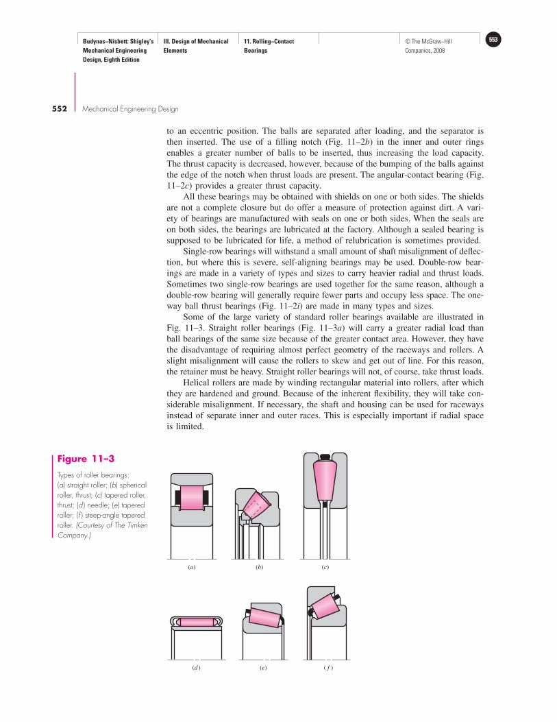
Budynas−Nisbett: Shigley’s
Mechanical Engineering
Design, Eighth Edition
III. Design of Mechanical
Elements
11. Rolling−Contact
Bearings
553© The McGraw−Hill
Companies, 2008
552 Mechanical Engineering Design
(a)
(d ) (e) ( f )
(b) (c)
Figure 11–3
Types of roller bearings:(a) straight roller; (b) sphericalroller, thrust; (c) tapered roller,thrust; (d ) needle; (e) taperedroller; (f ) steep-angle taperedroller. (Courtesy of The TimkenCompany.)
to an eccentric position. The balls are separated after loading, and the separator is
then inserted. The use of a filling notch (Fig. 11–2b) in the inner and outer rings
enables a greater number of balls to be inserted, thus increasing the load capacity.
The thrust capacity is decreased, however, because of the bumping of the balls against
the edge of the notch when thrust loads are present. The angular-contact bearing (Fig.
11–2c) provides a greater thrust capacity.
All these bearings may be obtained with shields on one or both sides. The shields
are not a complete closure but do offer a measure of protection against dirt. A vari-
ety of bearings are manufactured with seals on one or both sides. When the seals are
on both sides, the bearings are lubricated at the factory. Although a sealed bearing is
supposed to be lubricated for life, a method of relubrication is sometimes provided.
Single-row bearings will withstand a small amount of shaft misalignment of deflec-
tion, but where this is severe, self-aligning bearings may be used. Double-row bear-
ings are made in a variety of types and sizes to carry heavier radial and thrust loads.
Sometimes two single-row bearings are used together for the same reason, although a
double-row bearing will generally require fewer parts and occupy less space. The one-
way ball thrust bearings (Fig. 11–2i) are made in many types and sizes.
Some of the large variety of standard roller bearings available are illustrated in
Fig. 11–3. Straight roller bearings (Fig. 11–3a) will carry a greater radial load than
ball bearings of the same size because of the greater contact area. However, they have
the disadvantage of requiring almost perfect geometry of the raceways and rollers. A
slight misalignment will cause the rollers to skew and get out of line. For this reason,
the retainer must be heavy. Straight roller bearings will not, of course, take thrust loads.
Helical rollers are made by winding rectangular material into rollers, after which
they are hardened and ground. Because of the inherent flexibility, they will take con-
siderable misalignment. If necessary, the shaft and housing can be used for raceways
instead of separate inner and outer races. This is especially important if radial space
is limited.

Budynas−Nisbett: Shigley’s
Mechanical Engineering
Design, Eighth Edition
III. Design of Mechanical
Elements
11. Rolling−Contact
Bearings
554 © The McGraw−Hill
Companies, 2008
Rolling-Contact Bearings 553
The spherical-roller thrust bearing (Fig. 11–3b) is useful where heavy loads and
misalignment occur. The spherical elements have the advantage of increasing their
contact area as the load is increased.
Needle bearings (Fig. 11–3d) are very useful where radial space is limited. They
have a high load capacity when separators are used, but may be obtained without sep-
arators. They are furnished both with and without races.
Tapered roller bearings (Fig. 11–3e, f ) combine the advantages of ball and
straight roller bearings, since they can take either radial or thrust loads or any com-
bination of the two, and in addition, they have the high load-carrying capacity of
straight roller bearings. The tapered roller bearing is designed so that all elements in
the roller surface and the raceways intersect at a common point on the bearing axis.
The bearings described here represent only a small portion of the many available
for selection. Many special-purpose bearings are manufactured, and bearings are also
made for particular classes of machinery. Typical of these are:
• Instrument bearings, which are high-precision and are available in stainless steel and
high-temperature materials
• Nonprecision bearings, usually made with no separator and sometimes having split
or stamped sheet-metal races
• Ball bushings, which permit either rotation or sliding motion or both
• Bearings with flexible rollers
11–2 Bearing LifeWhen the ball or roller of rolling-contact bearings rolls, contact stresses occur on the
inner ring, the rolling element, and on the outer ring. Because the curvature of the
contacting elements in the axial direction is different from that in the radial direction,
the equations for these stresses are more involved than in the Hertz equations pre-
sented in Chapter 3. If a bearing is clean and properly lubricated, is mounted and
sealed against the entrance of dust and dirt, is maintained in this condition, and is
operated at reasonable temperatures, then metal fatigue will be the only cause of fail-
ure. Inasmuch as metal fatigue implies many millions of stress applications success-
fully endured, we need a quantitative life measure. Common life measures are
• Number of revolutions of the inner ring (outer ring stationary) until the first tangible
evidence of fatigue
• Number of hours of use at a standard angular speed until the first tangible evidence of
fatigue
The commonly used term is bearing life, which is applied to either of the measures just
mentioned. It is important to realize, as in all fatigue, life as defined above is a sto-
chastic variable and, as such, has both a distribution and associated statistical parame-
ters. The life measure of an individual bearing is defined as the total number of revo-
lutions (or hours at a constant speed) of bearing operation until the failure criterion is
developed. Under ideal conditions, the fatigue failure consists of spalling of the load-
carrying surfaces. The American Bearing Manufacturers Association (ABMA) standard
states that the failure criterion is the first evidence of fatigue. The fatigue criterion used
by the Timken Company laboratories is the spalling or pitting of an area of 0.01 in2.
Timken also observes that the useful life of the bearing may extend considerably beyond
this point. This is an operational definition of fatigue failure in rolling bearings.

Budynas−Nisbett: Shigley’s
Mechanical Engineering
Design, Eighth Edition
III. Design of Mechanical
Elements
11. Rolling−Contact
Bearings
555© The McGraw−Hill
Companies, 2008
554 Mechanical Engineering Design
log L
log F
0
Figure 11–4
Typical bearing load-lifelog-log curve.
The rating life is a term sanctioned by the ABMA and used by most manufactur-
ers. The rating life of a group of nominally identical ball or roller bearings is defined as
the number of revolutions (or hours at a constant speed) that 90 percent of a group of
bearings will achieve or exceed before the failure criterion develops. The terms minimum
life, L10 life, and B10 life are also used as synonyms for rating life. The rating life is the
10th percentile location of the bearing group’s revolutions-to-failure distribution.
Median life is the 50th percentile life of a group of bearings. The term average
life has been used as a synonym for median life, contributing to confusion. When many
groups of bearings are tested, the median life is between 4 and 5 times the L10 life.
11–3 Bearing Load Life at Rated ReliabilityWhen nominally identical groups are tested to the life-failure criterion at different
loads, the data are plotted on a graph as depicted in Fig. 11–4 using a log-log trans-
formation. To establish a single point, load F1 and the rating life of group one (L10)1
are the coordinates that are logarithmically transformed. The reliability associated with
this point, and all other points, is 0.90. Thus we gain a glimpse of the load-life func-
tion at 0.90 reliability. Using a regression equation of the form
F L1/a = constant (11–1)
the result of many tests for various kinds of bearings result in
• a = 3 for ball bearings
• a = 10/3 for roller bearings (cylindrical and tapered roller)
A bearing manufacturer may choose a rated cycle value of 106 revolutions (or in
the case of the Timken Company, 90(106) revolutions) or otherwise, as declared in
the manufacturer’s catalog to correspond to a basic load rating in the catalog for each
bearing manufactured, as their rating life. We shall call this the catalog load rating
and display it algebraically as C10, to denote it as the 10th percentile rating life for
a particular bearing in the catalog. From Eq. (11–1) we can write
F1L1/a
1 = F2L1/a
2 (11–2)
and associate load F1 with C10, life measure L1 with L10, and write
C10L1/a
10 = F L1/a
where the units of L are revolutions.

Budynas−Nisbett: Shigley’s
Mechanical Engineering
Design, Eighth Edition
III. Design of Mechanical
Elements
11. Rolling−Contact
Bearings
556 © The McGraw−Hill
Companies, 2008
Rolling-Contact Bearings 555
Further, we can write
C10(L RnR60)1/a = FD(L DnD60)1/a
catalog rating, lbf or kN desired speed, rev/min
rating life in hours desired life, hours
rating speed, rev/min desired radial load, lbf or kN
Solving for C10 gives
C10 = FD
(
L DnD60
L RnR60
)1/a
(11–3)
EXAMPLE 11–1 Consider SKF, which rates its bearings for 1 million revolutions, so that L10 life is
60L RnR = 106 revolutions. The L RnR60 product produces a familiar number. Timken,
for example, uses 90(106) revolutions. If you desire a life of 5000 h at 1725 rev/min
with a load of 400 lbf with a reliability of 90 percent, for which catalog rating would
you search in an SKF catalog?
Solution From Eq. (11–3),
C10 = FD
(
L DnD60
L RnR60
)1/a
= 400
[
5000(1725)60
106
]1/3
= 3211 lbf = 14.3 kN
If a bearing manufacturer rates bearings at 500 h at 33 13
rev/min with a reliability
of 0.90, then L RnR60 = 500(33 13)60 = 106 revolutions. The tendency is to substitute
106 for L RnR60 in Eq. (11–3). Although it is true that the 60 terms in Eq. (11–3) as
displayed cancel algebraically, they are worth keeping, because at some point in your
keystroke sequence on your hand-held calculator the manufacturer’s magic number
(106 or some other number) will appear to remind you of what the rating basis is and
those manufacturers’ catalogs to which you are limited. Of course, if you evaluate the
bracketed quantity in Eq. (11–3) by alternating between numerator and denominator
entries, the magic number will not appear and you will have lost an opportunity to check.
11–4 Bearing Survival: Reliability versus LifeAt constant load, the life measure distribution is right skewed as depicted in Fig. 11–5.
Candidates for a distributional curve fit include lognormal and Weibull. The Weibull is
by far the most popular, largely because of its ability to adjust to varying amounts of
skewness. If the life measure is expressed in dimensionless form as x = L/L10, then the
reliability can be expressed as [see Eq. (20–24), p. 970]
R = exp
[
−(
x − x0
θ − x0
)b]
(11–4)
where R = reliability
x = life measure dimensionless variate, L/L10
x0 = guaranteed, or “minimum,’’ value of the variate
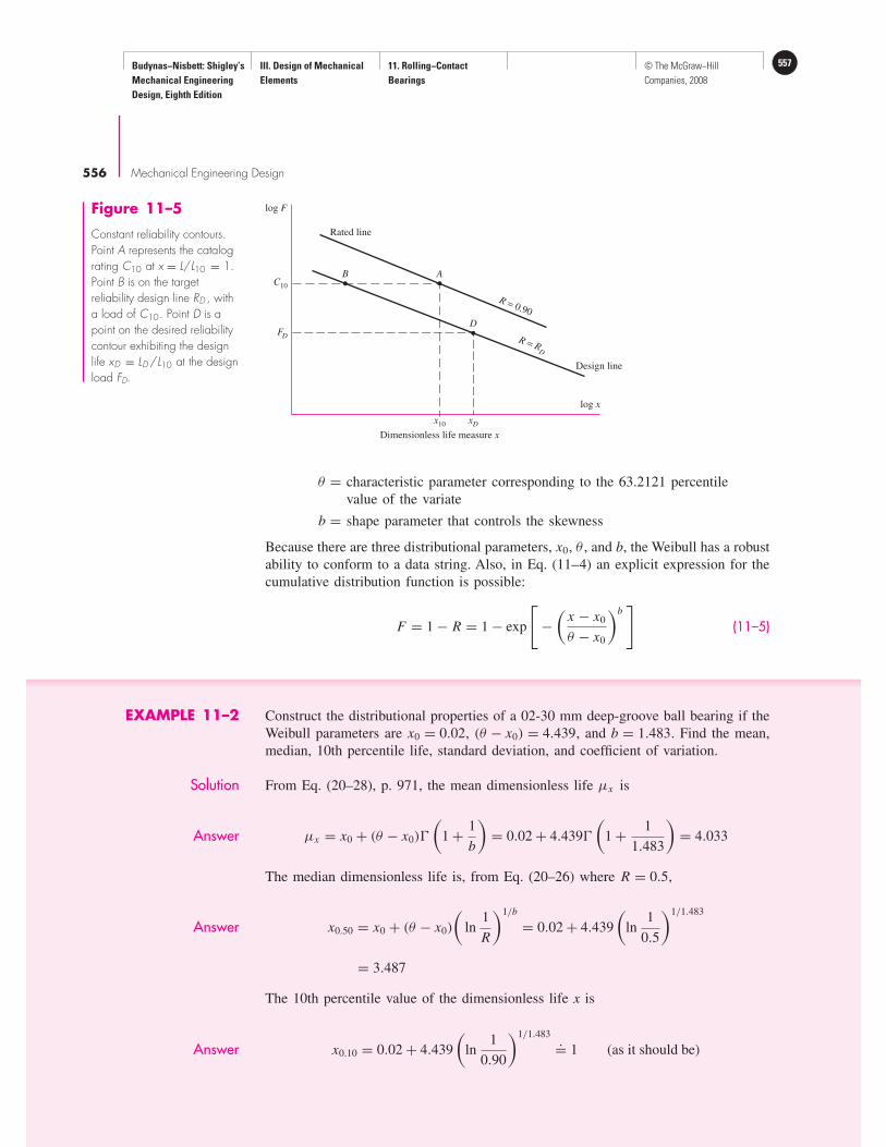
Budynas−Nisbett: Shigley’s
Mechanical Engineering
Design, Eighth Edition
III. Design of Mechanical
Elements
11. Rolling−Contact
Bearings
557© The McGraw−Hill
Companies, 2008
556 Mechanical Engineering Design
log x
log F
C10
FD
xDx10
Dimensionless life measure x
AB
Rated line
Design line
D
R = 0.90
R = RD
Figure 11–5
Constant reliability contours.Point A represents the catalograting C10 at x = L/L10 = 1.Point B is on the targetreliability design line RD , witha load of C10. Point D is apoint on the desired reliabilitycontour exhibiting the designlife xD = LD /L10 at the designload FD.
θ = characteristic parameter corresponding to the 63.2121 percentile
value of the variate
b = shape parameter that controls the skewness
Because there are three distributional parameters, x0, θ , and b, the Weibull has a robust
ability to conform to a data string. Also, in Eq. (11–4) an explicit expression for the
cumulative distribution function is possible:
F = 1 − R = 1 − exp
[
−(
x − x0
θ − x0
)b]
(11–5)
EXAMPLE 11–2 Construct the distributional properties of a 02-30 mm deep-groove ball bearing if the
Weibull parameters are x0 = 0.02, (θ − x0) = 4.439, and b = 1.483. Find the mean,
median, 10th percentile life, standard deviation, and coefficient of variation.
Solution From Eq. (20–28), p. 971, the mean dimensionless life µx is
Answer µx = x0 + (θ − x0)�
(
1 + 1
b
)
= 0.02 + 4.439�
(
1 + 1
1.483
)
= 4.033
The median dimensionless life is, from Eq. (20–26) where R = 0.5,
Answer x0.50 = x0 + (θ − x0)
(
ln1
R
)1/b
= 0.02 + 4.439
(
ln1
0.5
)1/1.483
= 3.487
The 10th percentile value of the dimensionless life x is
Answer x0.10 = 0.02 + 4.439
(
ln1
0.90
)1/1.483.= 1 (as it should be)

Budynas−Nisbett: Shigley’s
Mechanical Engineering
Design, Eighth Edition
III. Design of Mechanical
Elements
11. Rolling−Contact
Bearings
558 © The McGraw−Hill
Companies, 2008
Rolling-Contact Bearings 557
The standard deviation of the dimensionless life is given by Eq. (20–29):
Answer σx = (θ − x0)
[
�
(
1 + 2
b
)
− �2
(
1 + 1
b
)]1/2
= 4.439
[
�
(
1 + 2
1.483
)
− �2
(
1 + 1
1.483
)]1/2
= 2.753
The coefficient of variation of the dimensionless life is
Answer Cx = σx
µx
= 2.753
4.033= 0.683
11–5 Relating Load, Life, and ReliabilityThis is the designer’s problem. The desired load is not the manufacturer’s test load
or catalog entry. The desired speed is different from the vendor’s test speed, and the
reliability expectation is typically much higher than the 0.90 accompanying the catalog
entry. Figure 11–5 shows the situation. The catalog information is plotted as point A,
whose coordinates are (the logs of) C10 and x10 = L10/L10 = 1, a point on the 0.90
reliability contour. The design point is at D, with the coordinates (the logs of) FD
and xD , a point that is on the R = RD reliability contour. The designer must move
from point D to point A via point B as follows. Along a constant reliability contour
(B D), Eq. (11–2) applies:
FB x1/a
B = FDx1/a
D
from which
FB = FD
(
xD
xB
)1/a
(a)
Along a constant load line (AB), Eq. (11–4) applies:
RD = exp
[
−(
xB − x0
θ − x0
)b]
Solving for xB gives
xB = x0 + (θ − x0)
(
ln1
RD
)1/b
Now substitute this in Eq. (a) to obtain
FB = FD
(
xD
xB
)1/a
= FD
[
xD
x0 + (θ − x0)(ln 1/RD)1/b
]1/a
However, FB = C10, so
C10 = FD
[
xD
x0 + (θ − x0)(ln 1/RD)1/b
]1/a
(11–6)

Budynas−Nisbett: Shigley’s
Mechanical Engineering
Design, Eighth Edition
III. Design of Mechanical
Elements
11. Rolling−Contact
Bearings
559© The McGraw−Hill
Companies, 2008
558 Mechanical Engineering Design
As useful as Eq. (11–6) is, one’s attention to keystrokes and their sequence on a hand-
held calculator strays, and, as a result, the most common error is keying in the
inappropriate logarithm. We have the opportunity here to make Eq. (11–6) more error-
proof. Note that
ln1
RD
= ln1
1 − p f
= ln(1 + p f + · · ·) .= p f = 1 − RD
where p f is the probability for failure. Equation (11–6) can be written as
C10.= FD
[
xD
x0 + (θ − x0)(1 − RD)1/b
]1/a
R ≥ 0.90 (11–7)
Loads are often nonsteady, so that the desired load is multiplied by an applica-
tion factor a f . The steady load a f FD does the same damage as the variable load FD
does to the rolling surfaces. This point will be elaborated later.
EXAMPLE 11–3 The design load on a ball bearing is 413 lbf and an application factor of 1.2 is appro-
priate. The speed of the shaft is to be 300 rev/min, the life to be 30 kh with a reliability
of 0.99. What is the C10 catalog entry to be sought (or exceeded) when searching for a
deep-groove bearing in a manufacturer’s catalog on the basis of 106 revolutions for rat-
ing life? The Weibull parameters are x0 = 0.02, (θ − x0) = 4.439, and b = 1.483.
Solution xD = L
L10
= 60L DnD
60L RnR
= 60(30 000)300
106= 540
Thus, the design life is 540 times the L10 life. For a ball bearing, a = 3. Then, from
Eq. (11–7),
Answer C10 = (1.2)(413)
[
540
0.02 + 4.439(1 − 0.99)1/1.483
]1/3
= 6696 lbf
We have learned to identify the catalog basic load rating corresponding to a steady
radial load FD , a desired life L D , and a speed nD .
Shafts generally have two bearings. Often these bearings are different. If the bear-
ing reliability of the shaft with its pair of bearings is to be R, then R is related to the
individual bearing reliabilities RA and RB by
R = RA RB
First, we observe that if the product RA RB equals R, then, in general, RA and RB are
both greater than R. Since the failure of either or both of the bearings results in the
shutdown of the shaft, then A or B or both can create a failure. Second, in sizing bear-
ings one can begin by making RA and RB equal to the square root of the reliability
goal,√
R. In Ex. 11–3, if the bearing was one of a pair, the reliability goal would be√0.99, or 0.995. The bearings selected are discrete in their reliability property in your
problem, so the selection procedure “rounds up,” and the overall reliability exceeds
the goal R. Third, it may be possible, if RA >√
R, to round down on B yet have the
product RA RB still exceed the goal R.
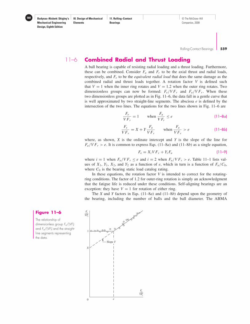
Budynas−Nisbett: Shigley’s
Mechanical Engineering
Design, Eighth Edition
III. Design of Mechanical
Elements
11. Rolling−Contact
Bearings
560 © The McGraw−Hill
Companies, 2008
Rolling-Contact Bearings 559
11–6 Combined Radial and Thrust LoadingA ball bearing is capable of resisting radial loading and a thrust loading. Furthermore,
these can be combined. Consider Fa and Fr to be the axial thrust and radial loads,
respectively, and Fe to be the equivalent radial load that does the same damage as the
combined radial and thrust loads together. A rotation factor V is defined such
that V = 1 when the inner ring rotates and V = 1.2 when the outer ring rotates. Two
dimensionless groups can now be formed: Fe/V Fr and Fa/V Fr . When these
two dimensionless groups are plotted as in Fig. 11–6, the data fall in a gentle curve that
is well approximated by two straight-line segments. The abscissa e is defined by the
intersection of the two lines. The equations for the two lines shown in Fig. 11–6 are
Fe
V Fr
= 1 whenFa
V Fr
≤ e (11–8a)
Fe
V Fr
= X + YFa
V Fr
whenFa
V Fr
> e (11–8b)
where, as shown, X is the ordinate intercept and Y is the slope of the line for
Fa/V Fr > e. It is common to express Eqs. (11–8a) and (11–8b) as a single equation,
Fe = X i V Fr + Yi Fa (11–9)
where i = 1 when Fa/V Fr ≤ e and i = 2 when Fa/V Fr > e. Table 11–1 lists val-
ues of X1, Y1, X2, and Y2 as a function of e, which in turn is a function of Fa/C0,
where C0 is the bearing static load catalog rating.
In these equations, the rotation factor V is intended to correct for the rotating-
ring conditions. The factor of 1.2 for outer-ring rotation is simply an acknowledgment
that the fatigue life is reduced under these conditions. Self-aligning bearings are an
exception: they have V = 1 for rotation of either ring.
The X and Y factors in Eqs. (11–8a) and (11–8b) depend upon the geometry of
the bearing, including the number of balls and the ball diameter. The ABMA
Fe
VFr
0 e
Fa
VFr
1
Slope Y
X
Figure 11–6
The relationship ofdimensionless group Fe/(VFr)and Fa/(VFr) and the straight-line segments representingthe data.

Budynas−Nisbett: Shigley’s
Mechanical Engineering
Design, Eighth Edition
III. Design of Mechanical
Elements
11. Rolling−Contact
Bearings
561© The McGraw−Hill
Companies, 2008
560 Mechanical Engineering Design
Fa/(VFr) � e Fa/(VFr) � e
Fa/C0 e X1 Y1 X2 Y2
0.014* 0.19 1.00 0 0.56 2.30
0.021 0.21 1.00 0 0.56 2.15
0.028 0.22 1.00 0 0.56 1.99
0.042 0.24 1.00 0 0.56 1.85
0.056 0.26 1.00 0 0.56 1.71
0.070 0.27 1.00 0 0.56 1.63
0.084 0.28 1.00 0 0.56 1.55
0.110 0.30 1.00 0 0.56 1.45
0.17 0.34 1.00 0 0.56 1.31
0.28 0.38 1.00 0 0.56 1.15
0.42 0.42 1.00 0 0.56 1.04
0.56 0.44 1.00 0 0.56 1.00
∗Use 0.014 if Fa C0 � 0.014.
Table 11–1
Equivalent Radial Load
Factors for Ball Bearings
recommendations are based on the ratio of the thrust component Fa to the basic static
load rating C0 and a variable reference value e. The static load rating C0 is tabulated,
along with the basic dynamic load rating C10, in many of the bearing manufacturers’
publications; see Table 11–2, for example.
Since straight or cylindrical roller bearings will take no axial load, or very little,
the Y factor is always zero.
The ABMA has established standard boundary dimensions for bearings, which
define the bearing bore, the outside diameter (OD), the width, and the fillet sizes on
the shaft and housing shoulders. The basic plan covers all ball and straight roller bear-
ings in the metric sizes. The plan is quite flexible in that, for a given bore, there is
an assortment of widths and outside diameters. Furthermore, the outside diameters
selected are such that, for a particular outside diameter, one can usually find a vari-
ety of bearings having different bores and widths.
This basic ABMA plan is illustrated in Fig. 11–7. The bearings are identified by a
two-digit number called the dimension-series code. The first number in the code is from
the width series, 0, 1, 2, 3, 4, 5, and 6. The second number is from the diameter series
012
3
4
Diameter
series
Dimension
series
Width series
Bore
OD
0 1 2 3
00
10
12
13
20
30
31
32
33
22
23
02
03
04
r
r
Figure 11–7
The basic ABMA plan forboundary dimensions. Theseapply to ball bearings, straightroller bearings, and sphericalroller bearings, but not to inch-series ball bearings or taperedroller bearings. The contourof the corner is not specified.It may be rounded orchamfered, but it must besmall enough to clear the filletradius specified in thestandards.

Budynas−Nisbett: Shigley’s
Mechanical Engineering
Design, Eighth Edition
III. Design of Mechanical
Elements
11. Rolling−Contact
Bearings
562 © The McGraw−Hill
Companies, 2008
Rolling-Contact Bearings 561
Fillet Shoulder Load Ratings, kN
Bore, OD, Width, Radius, Diameter, mm Deep Groove Angular Contact
mm mm mm mm dS dH C10 C0 C10 C0
10 30 9 0.6 12.5 27 5.07 2.24 4.94 2.12
12 32 10 0.6 14.5 28 6.89 3.10 7.02 3.05
15 35 11 0.6 17.5 31 7.80 3.55 8.06 3.65
17 40 12 0.6 19.5 34 9.56 4.50 9.95 4.75
20 47 14 1.0 25 41 12.7 6.20 13.3 6.55
25 52 15 1.0 30 47 14.0 6.95 14.8 7.65
30 62 16 1.0 35 55 19.5 10.0 20.3 11.0
35 72 17 1.0 41 65 25.5 13.7 27.0 15.0
40 80 18 1.0 46 72 30.7 16.6 31.9 18.6
45 85 19 1.0 52 77 33.2 18.6 35.8 21.2
50 90 20 1.0 56 82 35.1 19.6 37.7 22.8
55 100 21 1.5 63 90 43.6 25.0 46.2 28.5
60 110 22 1.5 70 99 47.5 28.0 55.9 35.5
65 120 23 1.5 74 109 55.9 34.0 63.7 41.5
70 125 24 1.5 79 114 61.8 37.5 68.9 45.5
75 130 25 1.5 86 119 66.3 40.5 71.5 49.0
80 140 26 2.0 93 127 70.2 45.0 80.6 55.0
85 150 28 2.0 99 136 83.2 53.0 90.4 63.0
90 160 30 2.0 104 146 95.6 62.0 106 73.5
95 170 32 2.0 110 156 108 69.5 121 85.0
Table 11–2
Dimensions and Load Ratings for Single-Row 02-Series Deep-Groove and Angular-Contact Ball Bearings
(outside), 8, 9, 0, 1, 2, 3, and 4. Figure 11–7 shows the variety of bearings that may be
obtained with a particular bore. Since the dimension-series code does not reveal the
dimensions directly, it is necessary to resort to tabulations. The 02 series is used here as
an example of what is available. See Table 11–2.
The housing and shaft shoulder diameters listed in the tables should be used
whenever possible to secure adequate support for the bearing and to resist the maxi-
mum thrust loads (Fig. 11–8). Table 11–3 lists the dimensions and load ratings of
some straight roller bearings.
To assist the designer in the selection of bearings, most of the manufacturers’
handbooks contain data on bearing life for many classes of machinery, as well as
information on load-application factors. Such information has been accumulated the
hard way, that is, by experience, and the beginner designer should utilize this
information until he or she gains enough experience to know when deviations are pos-
sible. Table 11–4 contains recommendations on bearing life for some classes of
machinery. The load-application factors in Table 11–5 serve the same purpose as fac-
tors of safety; use them to increase the equivalent load before selecting a bearing.

Budynas−Nisbett: Shigley’s
Mechanical Engineering
Design, Eighth Edition
III. Design of Mechanical
Elements
11. Rolling−Contact
Bearings
563© The McGraw−Hill
Companies, 2008
562 Mechanical Engineering Design
02-Series 03-Series
Bore, OD, Width, Load Rating, kN OD, Width, Load Rating, kN
mm mm mm C10 C0 mm mm C10 C0
25 52 15 16.8 8.8 62 17 28.6 15.0
30 62 16 22.4 12.0 72 19 36.9 20.0
35 72 17 31.9 17.6 80 21 44.6 27.1
40 80 18 41.8 24.0 90 23 56.1 32.5
45 85 19 44.0 25.5 100 25 72.1 45.4
50 90 20 45.7 27.5 110 27 88.0 52.0
55 100 21 56.1 34.0 120 29 102 67.2
60 110 22 64.4 43.1 130 31 123 76.5
65 120 23 76.5 51.2 140 33 138 85.0
70 125 24 79.2 51.2 150 35 151 102
75 130 25 93.1 63.2 160 37 183 125
80 140 26 106 69.4 170 39 190 125
85 150 28 119 78.3 180 41 212 149
90 160 30 142 100 190 43 242 160
95 170 32 165 112 200 45 264 189
100 180 34 183 125 215 47 303 220
110 200 38 229 167 240 50 391 304
120 215 40 260 183 260 55 457 340
130 230 40 270 193 280 58 539 408
140 250 42 319 240 300 62 682 454
150 270 45 446 260 320 65 781 502
Table 11–3
Dimensions and Basic Load Ratings for Cylindrical Roller Bearings
dSdH
Figure 11–8
Shaft and housing shoulderdiameters dS and dH shouldbe adequate to ensure goodbearing support.

Budynas−Nisbett: Shigley’s
Mechanical Engineering
Design, Eighth Edition
III. Design of Mechanical
Elements
11. Rolling−Contact
Bearings
564 © The McGraw−Hill
Companies, 2008
Rolling-Contact Bearings 563
Type of Application Life, kh
Instruments and apparatus for infrequent use Up to 0.5
Aircraft engines 0.5–2
Machines for short or intermittent operation where serviceinterruption is of minor importance 4–8
Machines for intermittent service where reliable operationis of great importance 8–14
Machines for 8-h service that are not always fully utilized 14–20
Machines for 8-h service that are fully utilized 20–30
Machines for continuous 24-h service 50–60
Machines for continuous 24-h service where reliability isof extreme importance 100–200
Table 11–4
Bearing-Life
Recommendations
for Various Classes
of Machinery
The static load rating is given in bearing catalog tables. It comes from the equations
C0 = Mnbd2b (ball bearings)
and
C0 = Mnr lcd (roller bearings)
where C0 = bearing static load rating, lbf (kN)
nb = number of balls
nr = number of rollers
db = diameter of balls, in (mm)
d = diameter of rollers, in (mm)
lc = length of contact line, in (mm)
and M takes on the values of which the following table is representative:
M in and lbf mm and kN
Radial ball 1.78(10)3 5.11(10)3
Ball thrust 7.10(10)3 20.4(10)3
Radial roller 3.13(10)3 8.99(10)3
Roller thrust 14.2(10)3 40.7(10)3
Type of Application Load Factor
Precision gearing 1.0–1.1
Commercial gearing 1.1–1.3
Applications with poor bearing seals 1.2
Machinery with no impact 1.0–1.2
Machinery with light impact 1.2–1.5
Machinery with moderate impact 1.5–3.0
Table 11–5
Load-Application Factors
Budynas−Nisbett: Shigley’s
Mechanical Engineering
Design, Eighth Edition
III. Design of Mechanical
Elements
11. Rolling−Contact
Bearings
565© The McGraw−Hill
Companies, 2008
564 Mechanical Engineering Design
EXAMPLE 11–4 An SKF 6210 angular-contact ball bearing has an axial load Fa of 400 lbf and a radial
load Fr of 500 lbf applied with the outer ring stationary. The basic static load rating
C0 is 4450 lbf and the basic load rating C10 is 7900 lbf. Estimate the L10 life at a
speed of 720 rev/min.
Solution V = 1 and Fa/C0 = 400/4450 = 0.090. Interpolate for e in Table 11–1:
Fa/(V Fr ) = 400/[(1)500] = 0.8 > 0.285. Thus, interpolate for Y2:
From Eq. (11–9),
Fe = X2V Fr + Y2 Fa = 0.56(1)500 + 1.527(400) = 890.8 lbf
With L D = L10 and FD = Fe, solving Eq. (11–3) for L10 gives
Answer L10 = 60L RnR
60nD
(
C10
Fe
)a
= 106
60(720)
(
7900
890.8
)3
= 16 150 h
Fa/C0 Y2
0.084 1.55
0.090 Y2 from which Y2 = 1.527
0.110 1.45
Fa/C0 e
0.084 0.28
0.090 e from which e = 0.285
0.110 0.30
We now know how to combine a steady radial load and a steady thrust load into
an equivalent steady radial load Fe that inflicts the same damage per revolution as the
radial–thrust combination.
11–7 Variable LoadingBearing loads are frequently variable and occur in some identifiable patterns:
• Piecewise constant loading in a cyclic pattern
• Continuously variable loading in a repeatable cyclic pattern
• Random variation
Equation (11–1) can be written as
Fa L = constant = K (a)
Note that F may already be an equivalent steady radial load for a radial–thrust load com-
bination. Figure 11–9 is a plot of Fa as ordinate and L as abscissa for Eq. (a). If a load
level of F1 is selected and run to the failure criterion, then the area under the F1-L1 trace
is numerically equal to K. The same is true for a load level F2; that is, the area under the
F2-L2 trace is numerically equal to K. The linear damage theory says that in the case of
load level F1, the area from L = 0 to L = L A does damage measured by Fa1 L A = D.

Budynas−Nisbett: Shigley’s
Mechanical Engineering
Design, Eighth Edition
III. Design of Mechanical
Elements
11. Rolling−Contact
Bearings
566 © The McGraw−Hill
Companies, 2008
Rolling-Contact Bearings 565
L1 L2 L0
F 2a
F1a
F a
A B
Figure 11–9
Plot of Fa as ordinate and L asabscissa for Fa L = constant.The linear damage hypothesissays that in the case of loadF1, the area under the curvefrom L = 0 to L = LA is ameasure of the damageD = Fa
1 LA. The completedamage to failure is measuredby Ca
10 L B .
Consider the piecewise continuous cycle depicted in Fig. 11–10. The loads Fei
are equivalent steady radial loads for combined radial–thrust loads. The damage done
by loads Fe1, Fe2, and Fe3 is
D = Fae1l1 + Fa
e2l2 + Fae3l3 (b)
where li is the number of revolutions at life L i . The equivalent steady load Feq when
run for l1 + l2 + l3 revolutions does the same damage D. Thus
D = Faeq(l1 + l2 + l3) (c)
Equating Eqs. (b) and (c), and solving for Feq, we get
Feq =[
Fae1l1 + Fa
e2l2 + Fae3l3
l1 + l2 + l3
]1/a
=[
∑
fi Faei
]1/a
(11–10)
where fi is the fraction of revolution run up under load Fei . Since li can be expressed
as ni ti , where ni is the rotational speed at load Fei and ti is the duration of that speed,
then it follows that
Feq =[∑
ni ti Faei
∑
ni ti
]1/a
(11–11)
The character of the individual loads can change, so an application factor (a f ) can be
prefixed to each Fei as (a f i Fei )a ; then Eq. (11–10) can be written
Feq =[
∑
fi (a f i Fei )a]1/a
Leq = K
Faeq
(11–12)
Fa
Fe2a
Fe1a
l1 l2 l3
l
F aeq
Fe3a
Figure 11–10
A three-part piecewise-continuous periodic loadingcycle involving loads Fe1, Fe2,and Fe3. Feq is the equivalentsteady load inflicting the samedamage when run for l1+l2 + l3 revolutions, doing thesame damage D per period.

Budynas−Nisbett: Shigley’s
Mechanical Engineering
Design, Eighth Edition
III. Design of Mechanical
Elements
11. Rolling−Contact
Bearings
567© The McGraw−Hill
Companies, 2008
566 Mechanical Engineering Design
EXAMPLE 11–5 A ball bearing is run at four piecewise continuous steady loads as shown in the fol-
lowing table. Columns (1), (2), and (5) to (8) are given.
Columns 1 and 2 are multiplied to obtain column 3. The column 3 entry is divided
by the sum of column 3, 2600, to give column 4. Columns 5, 6, and 7 are the radial,
axial, and equivalent loads respectively. Column 8 is the appropriate application fac-
tor. Column 9 is the product of columns 7 and 8.
Solution From Eq. (11–10), with a = 3, the equivalent radial load Fe is
Answer Fe =[
0.077(873)3 + 0.115(795)3 + 0.346(966)3 + 0.462(835)3]1/3 = 884 lbf
(1) (2) (3) (4) (5) (6) (7) (8) (9)
Product, TurnsTime Speed, Column Fraction, Fri, Fai, Fei, afi Fei,
Fraction rev/min (1) � (2) (3)/∑
(3) lbf lbf lbf afi lbf
0.1 2000 200 0.077 600 300 794 1.10 873
0.1 3000 300 0.115 300 300 626 1.25 795
0.3 3000 900 0.346 750 300 878 1.10 966
0.5 2400 1200 0.462 375 300 668 1.25 835
2600 1.000
Sometimes the question after several levels of loading is: How much life is left
if the next level of stress is held until failure? Failure occurs under the linear damage
hypothesis when the damage D equals the constant K = Fa L . Taking the first form
of Eq. (11–10), we write
FaeqLeq = Fa
e1l1 + Fae2l2 + Fa
e3l3
and note that
K = Fae1L1 = Fa
e2L2 = Fae3L3
and K also equals
K = Fae1l1 + Fa
e2l2 + Fae3l3 = K
L1
l1 + K
L2
l2 + K
L3
l3 = K∑ li
L i
From the outer parts of the preceding equation we obtain
∑ li
L i
= 1 (11–13)
This equation was advanced by Palmgren in 1924, and again by Miner in 1945. See
Eq. (6–58), p. 315.
The second kind of load variation mentioned is continuous, periodic variation,
depicted by Fig. 11–11. The differential damage done by Fa during rotation through
the angle dθ is
d D = Fadθ

Budynas−Nisbett: Shigley’s
Mechanical Engineering
Design, Eighth Edition
III. Design of Mechanical
Elements
11. Rolling−Contact
Bearings
568 © The McGraw−Hill
Companies, 2008
Rolling-Contact Bearings 567
Fa
Fa
0 �
d
Figure 11–11
A continuous load variation ofa cyclic nature whose periodis φ.
An example of this would be a cam whose bearings rotate with the cam through the
angle dθ . The total damage during a complete cam rotation is given by
D =∫
d D =∫ φ
0
Fadθ = Faeqφ
from which, solving for the equivalent load, we obtain
Feq =[
1
φ
∫ φ
0
Fadθ
]1/a
Leq = K
Faeq
(11–14)
The value of φ is often 2π , although other values occur. Numerical integration is often
useful to carry out the indicated integration, particularly when a is not an integer and
trigonometric functions are involved. We have now learned how to find the steady
equivalent load that does the same damage as a continuously varying cyclic load.
EXAMPLE 11–6 The operation of a particular rotary pump involves a power demand of P = P + A′
sin θ where P is the average power. The bearings feel the same variation as F =F + A sin θ . Develop an application factor a f for this application of ball bearings.
Solution From Eq. (11–14), with a = 3,
Feq =(
1
2π
∫ 2π
0
Fadθ
)1/a
=(
1
2π
∫ 2π
0
(F + A sin θ)3dθ
)1/3
=[
1
2π
(
∫ 2π
0
F3dθ + 3F2 A
∫ 2π
0
sin θ dθ + 3F A2
∫ 2π
0
sin2 θdθ
+ A3
∫ 2π
0
sin3 θ dθ
)]1/3
Feq =[
1
2π(2π F3 + 0 + 3π F A2 + 0)
]1/3
= F
[
1 + 3
2
(
A
F
)2]1/3
In terms of F , the application factor is
Answer a f =[
1 + 3
2
(
A
F
)2]1/3

Budynas−Nisbett: Shigley’s
Mechanical Engineering
Design, Eighth Edition
III. Design of Mechanical
Elements
11. Rolling−Contact
Bearings
569© The McGraw−Hill
Companies, 2008
We can present the result in tabular form:
A/F–
af
0 1
0.2 1.02
0.4 1.07
0.6 1.15
0.8 1.25
1.0 1.36
EXAMPLE 11–7 The second shaft on a parallel-shaft 25-hp foundry crane speed reducer contains a
helical gear with a pitch diameter of 8.08 in. Helical gears transmit components of
force in the tangential, radial, and axial directions (see Chap. 13). The components of
the gear force transmitted to the second shaft are shown in Fig. 11–12, at point A.
The bearing reactions at C and D, assuming simple-supports, are also shown. A ball
bearing is to be selected for location C to accept the thrust, and a cylindrical roller
11–8 Selection of Ball and Cylindrical Roller BearingsWe have enough information concerning the loading of rolling-contact ball and roller
bearings to develop the steady equivalent radial load that will do as much damage to
the bearing as the existing loading. Now let’s put it to work.
568 Mechanical Engineering Design
4.04 in
297.5
106.6
D
A
B
3 in
3 in
y
z
C
356.6
344
x
297.5
250
344
595
Figure 11–12
Forces in pounds applied tothe second shaft of the helicalgear speed reducer ofEx. 11–7.

Budynas−Nisbett: Shigley’s
Mechanical Engineering
Design, Eighth Edition
III. Design of Mechanical
Elements
11. Rolling−Contact
Bearings
570 © The McGraw−Hill
Companies, 2008
Rolling-Contact Bearings 569
bearing is to be utilized at location D. The life goal of the speed reducer is 10 kh, with
a reliability factor for the ensemble of all four bearings (both shafts) to equal or exceed
0.96 for the Weibull parameters of Ex. 11–3. The application factor is to be 1.2.
(a) Select the roller bearing for location D.
(b) Select the ball bearing (angular contact) for location C, assuming the inner ring
rotates.
Solution The torque transmitted is T = 595(4.04) = 2404 lbf · in. The speed at the rated horse-
power, given by Eq. (3–40), p. 138, is
nD = 63 025H
T= 63 025(25)
2404= 655.4 rev/min
The radial load at D is√
106.62 + 297.52 = 316.0 lbf, and the radial load at C is√356.62 + 297.52 = 464.4 lbf. The individual bearing reliabilities, if equal, must be
at least 4√
0.96 = 0.98985.= 0.99. The dimensionless design life for both bearings is
xD = L
L10
= 60L DnD
60L RnR
= 60(10 000)655.4
106= 393.2
(a) From Eq. (11–7), the Weibull parameters of Ex. 11–3, an application factor of 1.2,
and a = 10/3 for the roller bearing at D, the catalog rating should be equal to or
greater than
C10 = a f FD
[
xD
x0 + (θ − x0)(1 − RD)1/b
]1/a
= 1.2(316.0)
[
393.2
0.02 + 4.439(1 − 0.99)1/1.483
]3/10
= 3591 lbf = 16.0 kN
Answer The absence of a thrust component makes the selection procedure simple. Choose a
02-25 mm series, or a 03-25 mm series cylindrical roller bearing from Table 11–3.
(b) The ball bearing at C involves a thrust component. This selection procedure
requires an iterative procedure. Assuming Fa/(V Fr ) > e,
1 Choose Y2 from Table 11–1.
2 Find C10.
3 Tentatively identify a suitable bearing from Table 11–2, note C0.
4 Using Fa/C0 enter Table 11–1 to obtain a new value of Y2.
5 Find C10.
6 If the same bearing is obtained, stop.
7 If not, take next bearing and go to step 4.
As a first approximation, take the middle entry from Table 11–1:
X2 = 0.56 Y2 = 1.63.
From Eq. (11–8b), with V = 1,
Fe
V Fr
= X + Y
V
Fa
Fr
= 0.56 + 1.63344
(1)464.4= 1.77
Fe = 1.77V Fr = 1.77(1)464.4 = 822 lbf or 3.66 kN

Budynas−Nisbett: Shigley’s
Mechanical Engineering
Design, Eighth Edition
III. Design of Mechanical
Elements
11. Rolling−Contact
Bearings
571© The McGraw−Hill
Companies, 2008
570 Mechanical Engineering Design
From Eq. (11–7), with a = 3,
C10 = 1.2(3.66)
[
393.2
0.02 + 4.439(1 − 0.99)1/1.483
]1/3
= 53.4 kN
From Table 11–2, angular-contact bearing 02-60 mm has C10 = 55.9 kN. C0 is 35.5 kN.
Step 4 becomes, with Fa in kN,
Fa
C0
= 344(4.45)10−3
35.5= 0.0431
which makes e from Table 11–1 approximately 0.24. Now Fa/[V Fr ] = 344/[(1)
464.4] = 0.74, which is greater than 0.24, so we find Y2 by interpolation:
From Eq. (11–8b),
Fe
V Fr
= 0.56 + 1.84344
464.4= 1.92
Fe = 1.92V Fr = 1.92(1)464.4 = 892 lbf or 3.97 kN
The prior calculation for C10 changes only in Fe, so
C10 = 3.97
3.6653.4 = 57.9 kN
From Table 11–2 an angular contact bearing 02-65 mm has C10 = 63.7 kN and C0
of 41.5 kN. Again,
Fa
C0
= 344(4.45)10−3
41.5= 0.0369
making e approximately 0.23. Now from before, Fa/V Fr = 0.74, which is greater
than 0.23. We find Y2 again by interpolation:
From Eq. (11–8b),
Fe
V Fr
= 0.56 + 1.90344
464.4= 1.967
Fe = 1.967V Fr = 1.967(1)464.4 = 913.5 lbf or 4.065 kN
Fa/C0 Y2
0.028 1.99
0.0369 Y2 from which Y2 � 1.90
0.042 1.85
Fa/C0 Y2
0.042 1.85
0.043 Y2 from which Y2 � 1.84
0.056 1.71

Budynas−Nisbett: Shigley’s
Mechanical Engineering
Design, Eighth Edition
III. Design of Mechanical
Elements
11. Rolling−Contact
Bearings
572 © The McGraw−Hill
Companies, 2008
Rolling-Contact Bearings 571
The prior calculation for C10 changes only in Fe, so
C10 = 4.07
3.6653.4 = 59.4 kN
Answer From Table 11–2 an angular-contact 02-65 mm is still selected, so the iteration is complete.
11–9 Selection of Tapered Roller BearingsTapered roller bearings have a number of features that make them complicated. As we
address the differences between tapered roller and ball and cylindrical roller bearings,
note that the underlying fundamentals are the same, but that there are differences in
detail. Moreover, bearing and cup combinations are not necessarily priced in propor-
tion to capacity. Any catalog displays a mix of high-production, low-production, and
successful special-order designs. Bearing suppliers have computer programs that will
take your problem descriptions, give intermediate design assessment information, and
list a number of satisfactory cup-and-cone combinations in order of decreasing cost.
Company sales offices provide access to comprehensive engineering services to help
designers select and apply their bearings. At a large original equipment manufacturer’s
plant, there may be a resident bearing company representative.
Take a few minutes to go to your department’s design library and look at a bear-
ing supplier’s engineering catalog, such as The Timken Company’s Bearing Selection
Handbook—Revised (1986). There is a log of engineering information and detail,
based on long and successful experience. All we can do here is introduce the vocab-
ulary, show congruence to fundamentals that were learned earlier, offer examples, and
develop confidence. Finally, problems should reinforce the learning experience.
Form
The four components of a tapered roller bearing assembly are the
• Cone (inner ring)
• Cup (outer ring)
• Tapered rollers
• Cage (spacer-retainer)
The assembled bearing consists of two separable parts: (1) the cone assembly: the
cone, the rollers, and the cage; and (2) the cup. Bearings can be made as single-row,
two-row, four-row, and thrust-bearing assemblies. Additionally, auxiliary components
such as spacers and closures can be used.
A tapered roller bearing can carry both radial and thrust (axial) loads, or any com-
bination of the two. However, even when an external thrust load is not present, the radial
load will induce a thrust reaction within the bearing because of the taper. To avoid the
separation of the races and the rollers, this thrust must be resisted by an equal and oppo-
site force. One way of generating this force is to always use at least two tapered roller
bearings on a shaft. Two bearings can be mounted with the cone backs facing each other,
in a configuration called direct mounting, or with the cone fronts facing each other, in
what is called indirect mounting. Figure 11–13 shows the nomenclature of a tapered
roller bearing, and the point G through which radial and axial components of load act.

Budynas−Nisbett: Shigley’s
Mechanical Engineering
Design, Eighth Edition
III. Design of Mechanical
Elements
11. Rolling−Contact
Bearings
573© The McGraw−Hill
Companies, 2008
572 Mechanical Engineering Design
Cup o
uts
ide
dia
met
er (
OD
) D
Cone
bore
d
Cup back
face radius r
Cup back face
Cup front
face radius
Cup front face
Cage
Cone front faceCone back
face radius R
Standout F
Cone front
face rib
Cone front
face radius
Cone back face
Cone back face rib
Bearing width T
Cone length B
Cup
length C
G
a
Roller
Cup
Cone
Figure 11–13
Nomenclature of a taperedroller bearing. Point G is thelocation of the effective loadcenter; use this point toestimate the radial bearingload. (Courtesy of The TimkenCompany.)
A radial load will induce a thrust reaction. The load zone includes about half the
rollers and subtends an angle of approximately 180◦. Using the symbol Fa(180) for
the induced thrust load from a radial load with a 180◦ load zone, Timken provides
the equation
Fa(180) = 0.47Fr
K(11–15)
where the K factor is geometry-specific, coming from the relationship
K = 0.389 cot α
where α is half the included cup angle. The K factor is the ratio of the radial load rat-
ing to the thrust load rating. The K factor can be first approximated with 1.5 for a radial
bearing and 0.75 for a steep angle bearing in the preliminary selection process. After a
possible bearing is identified, the exact value of K for each bearing can be found in the
Bearing Selection Handbook—Revised (1986) in the case of Timken bearings.
Notation
The catalog rating C corresponding to 90 percent reliability was denoted C10 earlier
in the chapter, the subscript 10 denoting 10 percent failure level. Timken denoted its
catalog ratings as C90, the subscript 90 standing for “at 90 million revolutions.” The
failure fraction is still 10 percent (90 percent reliability). This should produce no dif-
ficulties since Timken’s catalog ratings for radial and thrust loads display neither C90
nor Ca(90) at the head of the columns. See Fig. 11–15, which is a reproduction of two
Timken catalog pages.

Budynas−Nisbett: Shigley’s
Mechanical Engineering
Design, Eighth Edition
III. Design of Mechanical
Elements
11. Rolling−Contact
Bearings
574 © The McGraw−Hill
Companies, 2008
Location of Reactions
Figure 11–14 shows a pair of tapered roller bearings mounted directly (b) and indi-
rectly (a) with the bearing reaction locations A0 and B0 shown for the shaft. For the
shaft as a beam, the span is ae, the effective spread. It is through points A0 and B0
that the radial loads act perpendicular to the shaft axis, and the thrust loads act along
the shaft axis. The geometric spread ag for the direct mounting is greater than for the
indirect mounting. With indirect mounting the bearings are closer together compared
to the direct mounting; however, the system stability is the same (ae is the same in
both cases). Thus direct and indirect mounting involve space and compactness needed
or desired, but with the same system stability.
Relating Load, Life, and Reliability
Recall Eq. (11–7) for a three-parameter Weibull model,
C10 = FD
[
xD
x0 + (θ − x0) (1 − RD)1/b
]1/a
Solving for xD gives
xD = x0 + (θ − x0)(1 − RD)1/b
(
C10
FD
)a
Rolling-Contact Bearings 573
Ac
Ao
Ac
a aae
ae
ag
ag
90°
Bearing A
Direct mounting
Indirect mounting
Bearing B
Bc
Bc
Bo
(a)
(b)
Figure 11–14
Comparison of mountingstability between indirect anddirect mountings. (Courtesy ofThe Timken Company.)

Budynas−Nisbett: Shigley’s
Mechanical Engineering
Design, Eighth Edition
III. Design of Mechanical
Elements
11. Rolling−Contact
Bearings
575© The McGraw−Hill
Companies, 2008
52.0002.0472
52.0002.0472
52.0002.0472
62.0002.4409
62.0002.4409
50.0051.9687
50.0051.9687
50.0051.9687
50.2921.9800
50.2921.9800
51.9942.0470
56.8962.2400
57.1502.2500
58.7382.3125
59.5302.3437
60.3252.3750
61.9122.4375
62.0002.4409
62.0002.4409
62.0002.4409
62.0002.4409
63.5002.5000
63.5002.5000
64.2922.5312
16.2500.6398
19.2500.7579
22.0000.8661
18.2500.7185
25.2500.9941
13.4950.5313
13.4950.5313
13.4950.5313
14.2240.5600
14.2240.5600
15.0110.5910
19.3680.7625
19.4310.7650
19.0500.7500
23.3680.9200
19.8420.7812
19.0500.7500
19.0500.7500
19.0500.7500
19.0500.7500
20.6380.8125
20.6380.8125
20.6380.8125
21.4330.8438
1.00.04
1.00.04
1.00.04
1.50.06
1.50.06
1.50.06
1.00.04
1.50.06
3.50.14
1.30.05
1.00.04
0.80.03
1.50.06
1.30.05
0.80.03
1.30.05
0.80.03
3.50.14
0.80.03
1.50.06
0.80.03
0.80.03
0.80.03
1.50.06
15.0000.5906
18.0000.7087
22.0000.8661
17.0000.6693
24.0000.9449
14.2600.5614
14.2600.5614
14.2600.5614
14.7320.5800
14.7320.5800
14.2600.5614
19.8370.7810
19.4310.7650
19.3550.7620
23.1140.9100
17.4620.6875
20.6380.8125
20.6380.8125
20.6380.8125
20.6380.8125
20.6380.8125
20.6380.8125
20.6380.8125
21.4330.8438
30.51.20
34.01.34
34.01.34
32.51.28
35.01.38
31.51.24
30.51.20
31.51.24
36.01.42
31.51.24
30.51.20
30.51.20
36.01.42
32.51.28
36.01.42
32.51.28
32.51.28
38.01.50
32.51.28
34.01.34
32.51.28
32.51.28
32.51.28
38.01.50
29.01.14
31.01.22
30.51.20
30.01.18
31.51.24
29.51.16
29.51.16
29.51.16
29.51.16
29.51.16
29.51.16
30.01.18
33.01.30
30.51.20
32.51.27
30.51.20
31.51.24
31.51.24
31.51.24
31.51.24
31.51.24
31.51.24
31.51.24
36.51.44
1.00.04
1.00.04
1.00.04
1.50.06
1.50.06
1.00.04
1.00.04
1.00.04
1.30.05
1.30.05
1.30.05
1.30.05
1.50.06
1.30.05
1.50.06
1.50.06
2.00.08
1.30.05
1.30.05
1.30.05
1.30.05
1.30.05
1.50.06
1.50.06
13.0000.5118
15.0000.5906
18.0000.7087
15.0000.5906
20.0000.7874
9.5250.3750
9.5250.3750
9.5250.3750
10.6680.4200
10.6680.4200
12.7000.5000
15.8750.6250
14.7320.5800
15.0800.5937
18.2880.7200
15.8750.6250
14.2880.5625
14.2880.5625
14.2880.5625
14.2880.5625
15.8750.6250
15.8750.6250
15.8750.6250
16.6700.6563
46.01.81
43.51.71
44.51.75
55.02.17
54.02.13
44.51.75
44.51.75
44.51.75
44.51.75
44.51.75
45.01.77
49.01.93
48.51.91
52.02.05
49.51.95
51.02.01
54.02.13
55.02.17
55.02.17
55.02.17
55.02.17
56.02.20
55.02.17
54.02.13
48.51.91
49.51.95
49.01.93
57.02.24
57.02.24
47.01.85
47.01.85
47.01.85
47.01.85
47.01.85
48.01.89
51.02.01
54.02.13
54.02.13
56.02.20
54.02.13
58.02.28
58.02.28
58.02.28
58.02.28
58.02.28
59.02.32
59.02.32
61.02.40
81901840
95202140
132002980
130002930
174003910
69901570
69901570
69901570
72101620
72101620
69901570
109002450
117002620
116002610
139003140
110002480
121002730
121002730
121002730
121002730
121002730
121002730
121002730
145003250
52601180
95102140
79601790
66801500
89302010
48101080
48101080
48101080
46201040
46201040
48101080
57401290
109002450
65601470
130002930
65501470
72801640
72801640
72801640
72801640
72801640
72801640
72801640
135003040
−3.6−0.14
−3.0−0.12
−7.6−0.30
−5.1−0.20
−9.7−0.38
−2.8−0.11
−2.8−0.11
−2.8−0.11
−3.3−0.13
−3.3−0.13
−2.8−0.11
−6.9−0.27
−3.0−0.12
−5.8−0.23
−5.1−0.20
−5.1−0.20
−5.8−0.23
−5.8−0.23
−5.8−0.23
−5.8−0.23
−5.8−0.23
−5.8−0.23
−5.8−0.23
−3.3−0.13
1.56
1.00
1.66
1.95
1.95
1.45
1.45
1.45
1.56
1.56
1.45
1.90
1.07
1.77
1.07
1.69
1.67
1.67
1.67
1.67
1.67
1.67
1.67
1.07
bore
d D T K aNlbf
Nlbf
outsidediameter width
R B d b D b D ad a12 r C1
one-row
radialthrust
fac-tor
rating at500 rpm for
3000 hours L 10 eff.load
center
cone cup
part numbers maxshaftfillet
radiuswidth
backingshoulderdiameters
backingshoulderdiameters
maxhous-ing
filletradius
width
cone cup
25.0000.9843
25.0000.9843
25.0000.9843
25.0000.9843
25.0000.9843
25.1590.9905
25.4001.0000
25.4001.0000
25.4001.0000
25.4001.0000
25.4001.0000
25.4001.0000
25.4001.0000
25.4001.0000
25.4001.0000
25.4001.0000
25.4001.0000
25.4001.0000
25.4001.0000
25.4001.0000
25.4001.0000
25.4001.0000
25.4001.0000
25.4001.0000
SINGLE-ROW STRAIGHT BORE
30205
32205-B
33205
30305
32305
07096
07100
07100-S
L44642
L44643
07100
1780
M84548
1986
M84249
15578
15101
15100
15101
15102
15101
15101
15101
M86643
30205
32205-B
33205
30305
32305
07196
07196
07196
L44610
.L44610
07204
1729
M84510
1932
M84210
15523
15243
15245
15245
15245
15244
15250
15250X
M86610
Figure 11–15
Catalog entry of single-row straight-bore Timken roller bearings, in part. (Courtesy of The Timken Company.)
574 Mechanical Engineering Design

Budynas−Nisbett: Shigley’s
Mechanical Engineering
Design, Eighth Edition
III. Design of Mechanical
Elements
11. Rolling−Contact
Bearings
576 © The McGraw−Hill
Companies, 2008
Rolling-Contact Bearings 575
65.0882.5625
66.4212.6150
68.2622.6875
72.2332.8438
72.6262.8593
62.0002.4409
63.1002.4843
66.4212.6150
58.7382.3125
50.2921.9800
60.3252.3750
62.0002.4409
66.4212.6150
56.8962.2400
57.1502.2500
58.7382.3125
58.7382.3125
60.3252.3750
60.3252.3750
22.2250.8750
23.8120.9375
22.2250.8750
25.4001.0000
30.1621.1875
19.0500.7500
23.8120.9375
23.8120.9375
19.0500.7500
14.2240.5600
19.8420.7812
19.0500.7500
23.8120.9375
19.8450.7813
17.4620.6875
19.0500.7500
19.0500.7500
19.8420.7812
19.8450.7813
23100
2687
02473
HM88630
3189
15103
2682
2682
1987
L44649
15580
15106
2688
1985
15590
1985
1988
15590
1985
23256
2631
02420
HM88610
3120
15245
2630
2631
1932
L44610
15523
15245
2631
1930
15520
1932
1932
15523
1931
1.50.06
1.30.05
0.80.03
0.80.03
0.80.03
0.80.03
1.50.06
1.50.06
0.80.03
3.50.14
3.50.14
0.80.03
1.50.06
0.80.03
3.50.14
0.80.03
3.50.14
3.50.14
0.50.03
21.4630.8450
25.4331.0013
22.2250.8750
25.4001.0000
29.9971.1810
20.6380.8125
25.4331.0013
25.4331.0013
19.3550.7620
14.7320.5800
17.4620.6875
20.6380.8125
25.4331.0013
19.3550.7620
17.4620.6875
19.3550.7620
19.3550.7620
17.4620.6875
19.3550.7620
39.01.54
33.51.32
34.51.36
39.51.56
35.51.40
33.01.30
34.51.36
34.51.36
32.51.28
37.51.48
38.51.52
33.51.32
35.01.38
34.01.34
39.51.56
34.01.34
39.51.56
39.51.56
34.01.34
34.51.36
31.51.24
33.51.32
39.51.56
35.01.38
32.51.28
32.01.26
32.01.26
31.51.24
31.01.22
32.01.26
33.01.30
33.01.30
33.51.32
33.51.32
33.51.32
33.51.32
33.51.32
33.51.32
1.50.06
1.30.05
1.50.06
2.30.09
3.30.13
1.30.05
0.80.03
1.30.05
1.30.05
1.30.05
1.50.06
1.30.05
1.30.05
0.80.03
1.50.06
1.30.05
1.30.05
1.50.06
1.30.05
15.8750.6250
19.0500.7500
17.4620.6875
19.8420.7812
23.8120.9375
14.2880.5625
19.0500.7500
19.0500.7500
15.0800.5937
10.6680.4200
15.8750.6250
14.2880.5625
19.0500.7500
15.8750.6250
13.4950.5313
15.0800.5937
15.0800.5937
15.8750.6250
15.8750.6250
53.02.09
58.02.28
59.02.32
60.02.36
61.02.40
55.02.17
57.02.24
58.02.28
52.02.05
44.51.75
51.02.01
55.02.17
58.02.28
51.02.01
51.02.01
52.02.05
52.02.05
51.02.01
52.02.05
63.02.48
60.02.36
63.02.48
69.02.72
67.02.64
58.02.28
59.02.32
60.02.36
54.02.13
47.01.85
54.02.13
58.02.28
60.02.36
54.02.11
53.02.09
54.02.13
54.02.13
54.02.13
55.02.17
131002950
184004140
153003440
184004140
227005110
121002730
184004140
184004140
116002610
72101620
110002480
121002730
184004140
116002610
110002480
116002610
116002610
110002480
116002610
164003690
80001800
109002450
172003870
130002910
72801640
80001800
80001800
65601470
46201040
65501470
72801640
80001800
65601470
65501470
65601470
65601470
65501470
65601470
−2.3−0.09
−9.4−0.37
−5.1−0.20
−4.6−0.18
−10.2−0.40
−5.8−0.23
−9.4−0.37
−9.4−0.37
−5.8−0.23
−3.3−0.13
−5.1−0.20
−5.8−0.23
−9.4−0.37
−5.8−0.23
−5.1−0.20
−5.8−0.23
−5.8−0.23
−5.1−0.20
−5.8−0.23
0.80
2.30
1.40
1.07
1.76
1.67
2.30
2.30
1.77
1.56
1.69
1.67
2.30
1.77
1.69
1.77
1.77
1.69
1.77
bore
d D T K aNlbf
Nlbf
outsidediameter width
R B d b D b D ad a12 r C1
one-row
radialthrust
fac-tor
rating at500 rpm for
3000 hours L 10 eff.load
center
cone cup
part numbers maxshaftfillet
radiuswidth
backingshoulderdiameters
backingshoulderdiameters
maxhous-ing
filletradius
width
cone cup
1
2
†
These maximum fillet radii will be cleared by the bearing corners.
Minus value indicates center is inside cone backface.
For standard class ONLY, the maximum metric size is a whole millimetre value.
For "J" part tolerances—see metric tolerances, page 73, and fitting practice, page 65.
ISO cone and cup combinations are designated with a common part number and should be purchased as an assembly.For ISO bearing tolerances—see metric tolerances, page 73, and fitting practice, page 65.
SINGLE-ROW STRAIGHT BORE
25.4001.0000
25.4001.0000
25.4001.0000
25.4001.0000
25.4001.0000
26.1571.0298
26.1621.0300
26.1621.0300
26.9751.0620
26.9881.0625
26.9881.0625
26.9881.0625
26.9881.0625
28.5751.1250
28.5751.1250
28.5751.1250
28.5751.1250
28.5751.1250
28.5751.1250
††
††
††
††
T C B
D
Db
d
db
Da
da
Ra
r
Figure 11–15
(Continued)
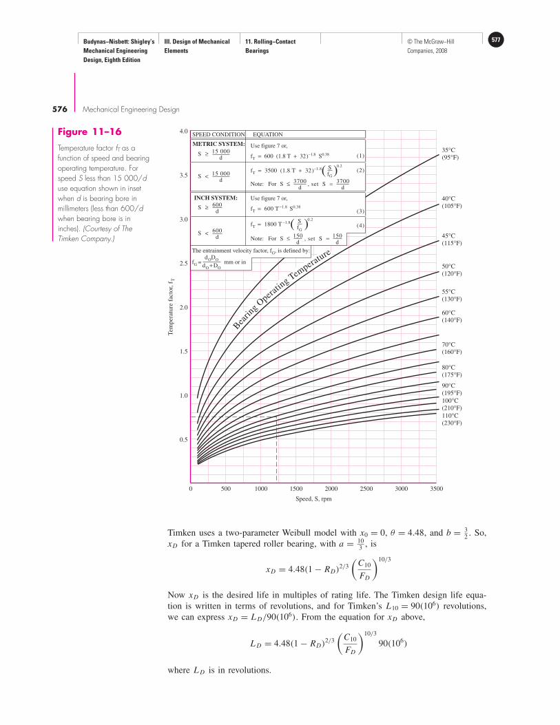
Budynas−Nisbett: Shigley’s
Mechanical Engineering
Design, Eighth Edition
III. Design of Mechanical
Elements
11. Rolling−Contact
Bearings
577© The McGraw−Hill
Companies, 2008
576 Mechanical Engineering Design
0 500 1000 1500 2000 2500 3000 3500
0.5
1.0
1.5
2.0
2.5
3.0
3.5
4.0
110°C
(230°F)
100°C
(210°F)
90°C
(195°F)
80°C
(175°F)
70°C
(160°F)
60°C
(140°F)
55°C
(130°F)
50°C
(120°F)
45°C
(115°F)
40°C
(105°F)
35°C
(95°F)
Speed, S, rpm
Tem
per
ature
fac
tor,
fT
SPEED CONDITION
METRIC SYSTEM:
INCH SYSTEM:
S ≥ 15 000
d
S ≥ 600
d
S < 600
d
S < 15 000
d
EQUATION
Use figure 7 or,
Use figure 7 or,
fT = 600 (1.8 T + 32)−1.8 S0.38
fT = 600 T −1.8 S0.38
fT = 3500 (1.8 T + 32)−1.8 SfG
0.2
( )Note: For S ≤
3700d
3700d
, set S =
Note: For S ≤150
d150
d, set S =
fT = 1800 T −1.8 SfG
0.2
( )
(1)
(2)
(3)
(4)
The entrainment velocity factor, fG, is defined by:
fG = mm or indODO
dO + DO
Bea
ri
ngO
perat
ing
Temperature
Figure 11–16
Temperature factor fT as afunction of speed and bearingoperating temperature. Forspeed S less than 15 000/duse equation shown in insetwhen d is bearing bore inmillimeters (less than 600/dwhen bearing bore is ininches). (Courtesy of TheTimken Company.)
Timken uses a two-parameter Weibull model with x0 = 0, θ = 4.48, and b = 32. So,
xD for a Timken tapered roller bearing, with a = 103
, is
xD = 4.48(1 − RD)2/3
(
C10
FD
)10/3
Now xD is the desired life in multiples of rating life. The Timken design life equa-
tion is written in terms of revolutions, and for Timken’s L10 = 90(106) revolutions,
we can express xD = L D/90(106). From the equation for xD above,
L D = 4.48(1 − RD)2/3
(
C10
FD
)10/3
90(106)
where L D is in revolutions.

Budynas−Nisbett: Shigley’s
Mechanical Engineering
Design, Eighth Edition
III. Design of Mechanical
Elements
11. Rolling−Contact
Bearings
578 © The McGraw−Hill
Companies, 2008
Rolling-Contact Bearings 577
Timken writes this equation as
L D = a1a2a3a4
(
C10
FD
)10/3
90(106) (11–16)
4.48 (1 − RD)2/3 a4 = 1 (spall size is 0.01 in2)
bearing material a3 = a3ka3la3m
alignment
lubricant a3l = fT fv
load zone
Temperature factor fT can be found in Fig. 11–16, and viscosity factor fv can be
found in Fig. 11–17.
For the usual case, a2 = a3k = a3m = 1, and solving the preceding equation for
C10 gives
C10 = a f P
[
L D
4.48 fT fv(1 − RD)2/390(106)
]3/10
(L D in revolutions) (11–17)
where FD is replaced by a f P . The load P is the dynamic equivalent load of the com-
bination Fr and Fa of Sec. 11–6. The particular values of X and Y are given in
20 30 40 50 100 200 300 400 500 10000.8
0.9
1.0
1.1
1.2
1.3
1.4200 300 400 500 1000 2000 3000 4000100
Viscosity, centistokes (cSt) @ 40° C
Viscosity, Saybolt universal seconds (SUS) @ 100° F
Vis
co
sity
facto
r, f
V
Figure 11–17
Viscosity factor fV as a functionof oil viscosity. (This graphapplies to petroleum oilwith a viscosity index ofapproximately 90.) (Courtesyof The Timken Company.)
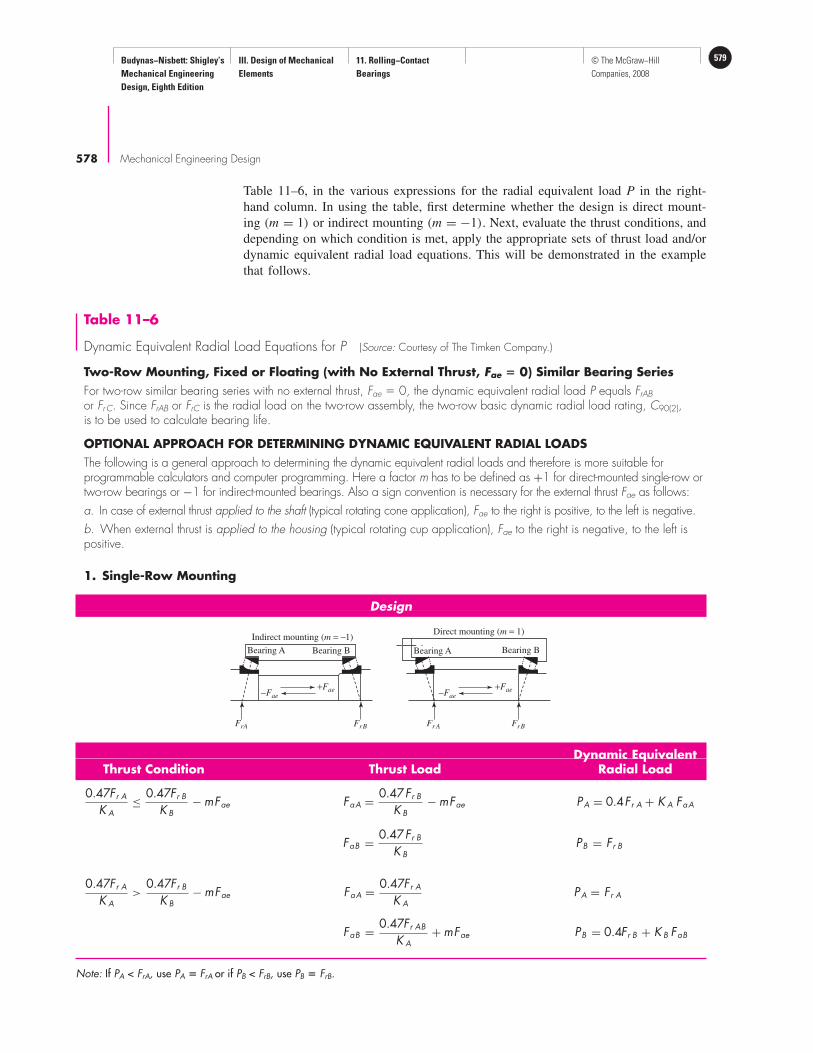
Budynas−Nisbett: Shigley’s
Mechanical Engineering
Design, Eighth Edition
III. Design of Mechanical
Elements
11. Rolling−Contact
Bearings
579© The McGraw−Hill
Companies, 2008
Table 11–6
Dynamic Equivalent Radial Load Equations for P (Source: Courtesy of The Timken Company.)
Two-Row Mounting, Fixed or Floating (with No External Thrust, Fae � 0) Similar Bearing Series
For two-row similar bearing series with no external thrust, Fae � 0, the dynamic equivalent radial load P equals FrAB
or FrC. Since FrAB or FrC is the radial load on the two-row assembly, the two-row basic dynamic radial load rating, C90(2),is to be used to calculate bearing life.
OPTIONAL APPROACH FOR DETERMINING DYNAMIC EQUIVALENT RADIAL LOADS
The following is a general approach to determining the dynamic equivalent radial loads and therefore is more suitable forprogrammable calculators and computer programming. Here a factor m has to be defined as +1 for direct-mounted single-row ortwo-row bearings or −1 for indirect-mounted bearings. Also a sign convention is necessary for the external thrust Fae as follows:
a. In case of external thrust applied to the shaft (typical rotating cone application), Fae to the right is positive, to the left is negative.
b. When external thrust is applied to the housing (typical rotating cup application), Fae to the right is negative, to the left ispositive.
1. Single-Row Mounting
Design
Indirect mounting (m = −1)
Bearing A Bearing B
−Fae
FrA FrB
+Fae
Direct mounting (m = 1)
Fr A FrB
−Fae
+Fae
Bearing A Bearing B
Table 11–6, in the various expressions for the radial equivalent load P in the right-
hand column. In using the table, first determine whether the design is direct mount-
ing (m = 1) or indirect mounting (m = −1). Next, evaluate the thrust conditions, and
depending on which condition is met, apply the appropriate sets of thrust load and/or
dynamic equivalent radial load equations. This will be demonstrated in the example
that follows.
Dynamic EquivalentThrust Condition Thrust Load Radial Load
0.47Fr A
K A≤ 0.47Fr B
K B− mFae FaA = 0.47Fr B
K B− mFae PA = 0.4Fr A + K A FaA
FaB = 0.47Fr B
K BPB = Fr B
0.47Fr A
K A>
0.47Fr B
K B− mFae FaA = 0.47Fr A
K APA = Fr A
FaB = 0.47Fr AB
K A+ mFae PB = 0.4Fr B + K B FaB
Note: If PA < FrA, use PA � FrA or if PB < FrB, use PB � FrB.
578 Mechanical Engineering Design
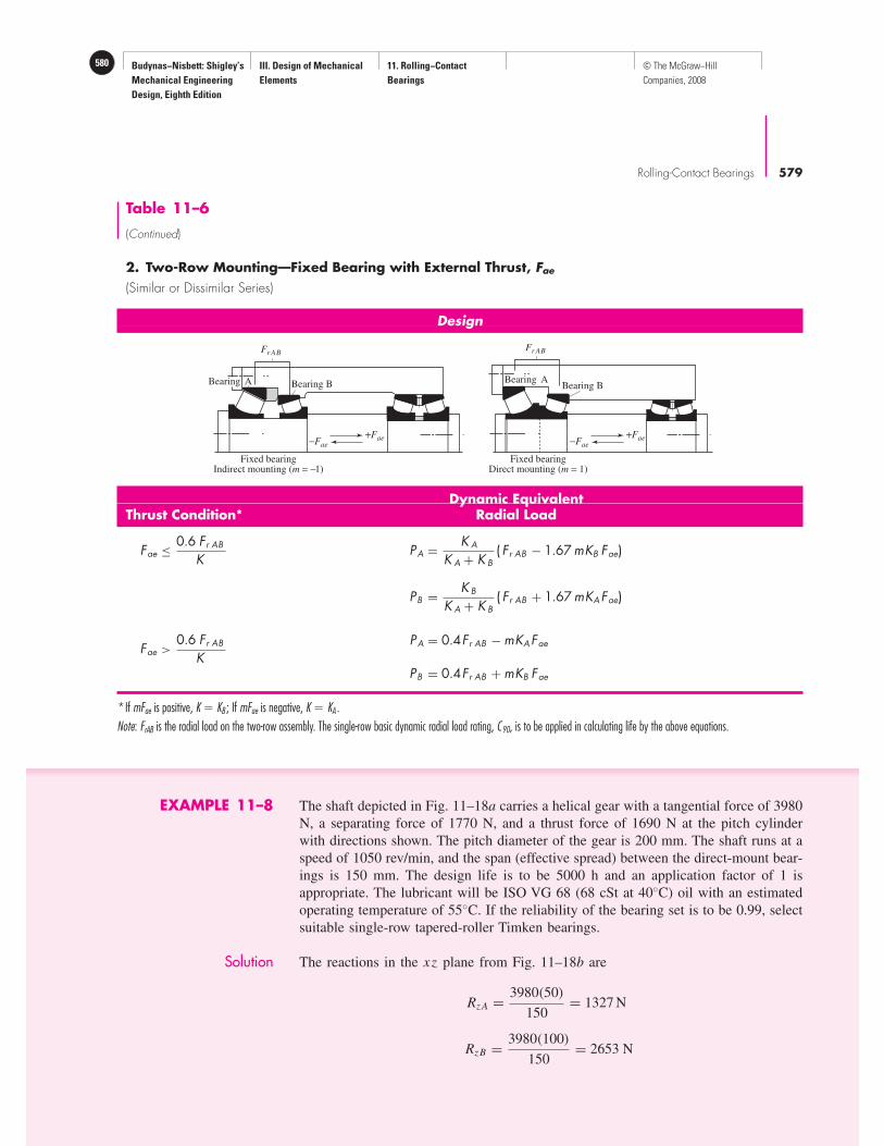
Budynas−Nisbett: Shigley’s
Mechanical Engineering
Design, Eighth Edition
III. Design of Mechanical
Elements
11. Rolling−Contact
Bearings
580 © The McGraw−Hill
Companies, 2008
2. Two-Row Mounting—Fixed Bearing with External Thrust, Fae
(Similar or Dissimilar Series)
Design
Dynamic EquivalentThrust Condition* Radial Load
Fae ≤ 0.6 Fr AB
KPA = K A
K A + K B( Fr AB − 1.67 mKB Fae)
PB = K B
K A + K B( Fr AB + 1.67 mKAFae)
Fae >0.6 Fr AB
KPA = 0.4Fr AB − mKAFae
PB = 0.4Fr AB + mKB Fae
*If mFae is positive, K � KB ; If mFae is negative, K � KA .
Note: FrAB is the radial load on the two-row assembly. The single-row basic dynamic radial load rating, C90, is to be applied in calculating life by the above equations.
Fr AB
Bearing A Bearing B
Fixed bearingIndirect mounting (m = −1)
Fixed bearingDirect mounting (m = 1)
Fr AB
Bearing ABearing B
−Fae
+Fae−Fae
+Fae
Table 11–6
(Continued)
Rolling-Contact Bearings 579
EXAMPLE 11–8 The shaft depicted in Fig. 11–18a carries a helical gear with a tangential force of 3980
N, a separating force of 1770 N, and a thrust force of 1690 N at the pitch cylinder
with directions shown. The pitch diameter of the gear is 200 mm. The shaft runs at a
speed of 1050 rev/min, and the span (effective spread) between the direct-mount bear-
ings is 150 mm. The design life is to be 5000 h and an application factor of 1 is
appropriate. The lubricant will be ISO VG 68 (68 cSt at 40◦C) oil with an estimated
operating temperature of 55◦C. If the reliability of the bearing set is to be 0.99, select
suitable single-row tapered-roller Timken bearings.
Solution The reactions in the xz plane from Fig. 11–18b are
Rz A = 3980(50)
150= 1327 N
RzB = 3980(100)
150= 2653 N
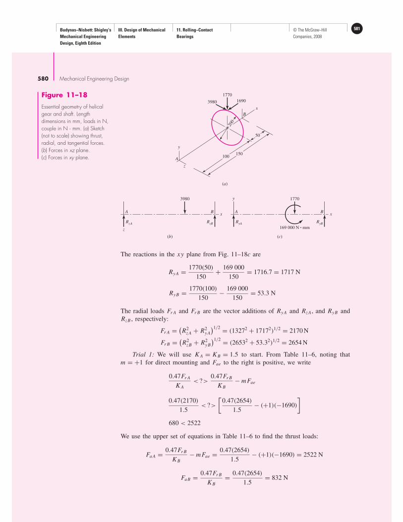
Budynas−Nisbett: Shigley’s
Mechanical Engineering
Design, Eighth Edition
III. Design of Mechanical
Elements
11. Rolling−Contact
Bearings
581© The McGraw−Hill
Companies, 2008
580 Mechanical Engineering Design
The reactions in the xy plane from Fig. 11–18c are
Ry A = 1770(50)
150+ 169 000
150= 1716.7 = 1717 N
Ry B = 1770(100)
150− 169 000
150= 53.3 N
The radial loads Fr A and Fr B are the vector additions of Ry A and Rz A , and Ry B and
RzB , respectively:
Fr A =(
R2z A + R2
y A
)1/2 = (13272 + 17172)1/2 = 2170 N
Fr B =(
R2zB + R2
y B
)1/2 = (26532 + 53.32)1/2 = 2654 N
Trial 1: We will use K A = K B = 1.5 to start. From Table 11–6, noting that
m = +1 for direct mounting and Fae to the right is positive, we write
0.47Fr A
K A
< ?>0.47Fr B
K B
− m Fae
0.47(2170)
1.5< ?>
[
0.47(2654)
1.5− (+1)(−1690)
]
680 < 2522
We use the upper set of equations in Table 11–6 to find the thrust loads:
Fa A = 0.47Fr B
K B
− m Fae = 0.47(2654)
1.5− (+1)(−1690) = 2522 N
FaB = 0.47Fr B
K B
= 0.47(2654)
1.5= 832 N
100
50
200
150
y
z
x
3980
1770
1690
(a)
(b)
3980
z
RzA
Ax
y
RzB
B
(c)
1770
RyA
Ax
RyB
B
B
A
169 000 N • mm
Figure 11–18
Essential geometry of helicalgear and shaft. Lengthdimensions in mm, loads in N,couple in N · mm. (a) Sketch(not to scale) showing thrust,radial, and tangential forces.(b) Forces in xz plane.(c) Forces in xy plane.
Budynas−Nisbett: Shigley’s
Mechanical Engineering
Design, Eighth Edition
III. Design of Mechanical
Elements
11. Rolling−Contact
Bearings
582 © The McGraw−Hill
Companies, 2008
Rolling-Contact Bearings 581
The dynamic equivalent loads PA and PB are
PA = 0.4Fr A + K A Fa A = 0.4(2170) + 1.5(2522) = 4651 N
PB = Fr B = 2654 N
From Fig. 11–16 for 1050 rev/min at 55◦C, fT = 1.31. From Fig. 11–17, fv = 1.01.
For use in Eq. (11–16), a3l = fT fv = 1.31(1.01) = 1.32. The catalog basic load rat-
ing corresponding to the load–life–reliability goals is given by Eq. (11–17). Estimate
RD as√
0.99 = 0.995 for each bearing. For bearing A, from Eq. (11–17) the catalog
entry C10 should equal or exceed
C10 = (1)(4651)
[
5000(1050)60
(4.48)1.32(1 − 0.995)2/390(106)
]3/10
= 11 466 N
From Fig. 11–14, tentatively select type TS 15100 cone and 15245 cup, which will
work: K A = 1.67, C10 = 12 100 N.
For bearing B, from Eq. (11–17), the catalog entry C10 should equal or exceed
C10 = (1)2654
[
5000(1050)60
(4.48)1.32(1 − 0.995)2/390(106)
]3/10
= 6543 N
Tentatively select the bearing identical to bearing A, which will work: K B = 1.67,
C10 = 12 100 N.
Trial 2: Use K A = K B = 1.67 from tentative bearing selection. The sense of the
previous inequality 680 < 2521 is still the same, so the same equations apply:
Fa A = 0.47Fr B
K B
− m Fae = 0.47(2654)
1.67− (+1)(−1690) = 2437 N
FaB = 0.47Fr B
K B
= 0.47(2654)
1.67= 747 N
PA = 0.4Fr A + K A Fa A = 0.4(2170) + 1.67(2437) = 4938 N
PB = Fr B = 2654 N
For bearing A, from Eq. (11–17) the corrected catalog entry C10 should equal or
exceed
C10 = (1)(4938)
[
5000(1050)60
(4.48)1.32(1 − 0.995)2/390(106)
]3/10
= 12 174 N
Although this catalog entry exceeds slightly the tentative selection for bearing A, we
will keep it since the reliability of bearing B exceeds 0.995. In the next section we
will quantitatively show that the combined reliability of bearing A and B will exceed
the reliability goal of 0.99.
For bearing B, PB = Fr B = 2654 N. From Eq. (11–17),
C10 = (1)2654
[
5000(1050)60
(4.48)1.32(1 − 0.995)2/390(106)
]3/10
= 6543 N
Select cone and cup 15100 and 15245, respectively, for both bearing A and B. Note
from Fig. 11–14 the effective load center is located at a = −5.8 mm, that is, 5.8 mm
into the cup from the back. Thus the shoulder-to-shoulder dimension should be
150 − 2(5.8) = 138.4 mm. Note, also, the calculation for the second bearing C10

Budynas−Nisbett: Shigley’s
Mechanical Engineering
Design, Eighth Edition
III. Design of Mechanical
Elements
11. Rolling−Contact
Bearings
583© The McGraw−Hill
Companies, 2008
582 Mechanical Engineering Design
contains the same bracketed expression as for the first. For example, on the first trial
C10 for bearing A is 11 466 N. C10 for bearing B can be easily calculated by
(C10)B = (C10)A
PA
PB = 11 466
46512654 = 6543 N
The computational effort can be simplified only after this is understood, and not until
then.
11–10 Design Assessment for Selected Rolling-Contact BearingsIn textbooks machine elements typically are treated singly. This can lead the reader
to the presumption that a design assessment involves only that element, in this case
a rolling-contact bearing. The immediately adjacent elements (the shaft journal and
the housing bore) have immediate influence on the performance. Other elements, fur-
ther removed (gears producing the bearing load), also have influence. Just as some
say, “If you pull on something in the environment, you find that it is attached to every-
thing else.” This should be intuitively obvious to those involved with machinery. How,
then, can one check shaft attributes that aren’t mentioned in a problem statement?
Possibly, because the bearing hasn’t been designed yet (in fine detail). All this points
out the necessary iterative nature of designing, say, a speed reducer. If power, speed,
and reduction are stipulated, then gear sets can be roughed in, their sizes, geometry,
and location estimated, shaft forces and moments identified, bearings tentatively
selected, seals identified; the bulk is beginning to make itself evident, the housing and
lubricating scheme as well as the cooling considerations become clearer, shaft over-
hangs and coupling accommodations appear. It is time to iterate, now addressing each
element again, knowing much more about all of the others. When you have completed
the necessary iterations, you will know what you need for the design assessment for
the bearings. In the meantime you do as much of the design assessment as you can,
avoiding bad selections, even if tentative. Always keep in mind that you eventually
have to do it all in order to pronounce your completed design satisfactory.
An outline of a design assessment for a rolling contact bearing includes, at a
minimum,
• Bearing reliability for the load imposed and life expected
• Shouldering on shaft and housing satisfactory
• Journal finish, diameter and tolerance compatible
• Housing finish, diameter and tolerance compatible
• Lubricant type according to manufacturer’s recommendations; lubricant paths and
volume supplied to keep operating temperature satisfactory
• Preloads, if required, are supplied
Since we are focusing on rolling-contact bearings, we can address bearing reliability
quantitatively, as well as shouldering. Other quantitative treatment will have to wait
until the materials for shaft and housing, surface quality, and diameters and tolerances
are known.
Budynas−Nisbett: Shigley’s
Mechanical Engineering
Design, Eighth Edition
III. Design of Mechanical
Elements
11. Rolling−Contact
Bearings
584 © The McGraw−Hill
Companies, 2008
Rolling-Contact Bearings 583
Bearing Reliability
Equation (11–6) can be solved for the reliability RD in terms of C10, the basic load
rating of the selected bearing:
R = exp
−
xD
(
a f FD
C10
)a
− x0
θ − x0
b
(11–18)
Equation (11–7) can likewise be solved for RD :
R.= 1 −
xD
(
a f FD
C10
)a
− x0
θ − x0
b
R ≥ 0.90 (11–19)
EXAMPLE 11–9 In Ex. 11–3, the minimum required load rating for 99 percent reliability, at xD =L/L10 = 540, is C10 = 6671 lbf = 29.7 kN. From Table 11–2 a 02-40 mm deep-
groove ball bearing would satisfy the requirement. If the bore in the application had
to be 70 mm or larger (selecting a 02-70 mm deep-groove ball bearing), what is the
resulting reliability?
Solution From Table 11–2, for a 02-70 mm deep-groove ball bearing, C10 = 61.8 kN = 13 888
lbf. Using Eq. (11–19), recalling from Ex. 11–3 that a f = 1.2, FD = 413 lbf,
x0 = 0.02, (θ − x0) = 4.439, and b = 1.489, we can write
Answer R.= 1 −
[
540
[
1.2(413)
13 888
]3
− 0.02
]
4.439
1.489
= 0.999 965
which, as expected, is much higher than 0.99 from Ex. 11–3.
In tapered roller bearings, or other bearings for a two-parameter Weibull distrib-
ution, Eq. (11–18) becomes, for x0 = 0, θ = 4.48, b = 32,
R = exp
{
−[
xD
θ(C10/[a f FD])a
]b }
= exp
{
−[
xD
4.48 fT fv(C10/[a f FD])10/3
]3/2 }
(11–20)
and Eq. (11–19) becomes
R.= 1 −
{
xD
θ[C10/(a f FD)]a
}b
= 1 −{
xD
4.48 fT fv[C10/(a f FD)]10/3
}3/2
(11–21)
Budynas−Nisbett: Shigley’s
Mechanical Engineering
Design, Eighth Edition
III. Design of Mechanical
Elements
11. Rolling−Contact
Bearings
585© The McGraw−Hill
Companies, 2008
584 Mechanical Engineering Design
EXAMPLE 11–10 In Ex. 11–8 bearings A and B (cone 15100 and cup 15245) have C10 = 12 100 N.
What is the reliability of the pair of bearings A and B?
Solution The desired life xD was 5000(1050)60/[90(106)] = 3.5 rating lives. Using Eq.
(11–21) for bearing A, where from Ex. 11–8, FD = PA = 4938 N, fT fv = 1.32, and
a f = 1, gives
RA.= 1 −
{
3.5
4.48(1.32) [12 100/ (1 × 4938)]10/3
}3/2
= 0.994 846
which is less than 0.995, as expected. Using Eq. (11–21) for bearing B with FD =PB = 2654 N gives
RB.= 1 −
{
3.5
4.48(1.32) [12 100/ (1 × 2654)]10/3
}3/2
= 0.999 769
Answer The reliability of the bearing pair is
R = RA RB = 0.994 846(0.999 769) = 0.994 616
which is greater than the overall reliability goal of 0.99. When two bearings are made
identical for simplicity, or reducing the number of spares, or other stipulation, and the
loading is not the same, both can be made smaller and still meet a reliability goal. If
the loading is disparate, then the more heavily loaded bearing can be chosen for a
reliability goal just slightly larger than the overall goal.
An additional example is useful to show what happens in cases of pure thrust
loading.
EXAMPLE 11–11 Consider a constrained housing as depicted in Fig. 11–19 with two direct-mount tapered
roller bearings resisting an external thrust Fae of 8000 N. The shaft speed is 950 rev/min,
the desired life is 10 000 h, the expected shaft diameter is approximately 1 in. The lubri-
cant is ISO VG 150 (150 cSt at 40◦C) oil with an estimated bearing operating tempera-
ture of 80◦C. The reliability goal is 0.95. The application factor is appropriately a f = 1.
(a) Choose a suitable tapered roller bearing for A.
(b) Choose a suitable tapered roller bearing for B.
(c) Find the reliabilities RA, RB , and R.
Solution (a) The bearing reactions at A are
Fr A = Fr B = 0
Fa A = Fae = 8000 N
Since bearing B is unloaded, we will start with R = RA = 0.95. From Table 11–6,
0.47Fr A
K A
< ?>0.47Fr B
K B
− m Fae
Budynas−Nisbett: Shigley’s
Mechanical Engineering
Design, Eighth Edition
III. Design of Mechanical
Elements
11. Rolling−Contact
Bearings
586 © The McGraw−Hill
Companies, 2008
Rolling-Contact Bearings 585
Noting that Fae to the right is positive (Table 11–6), with direct mounting m = +1,
we can write
0(0)
K A
< ?>
[
0.47(0)
K B
− (+1)(−8000)
]
0 < 8000 N
The top set of equations in Table 11–6 applies, so
Fa A = 0.47(0)
K B
− (+1)(−8000) = 8000 N
FaB = 0.47(0)
K B
= 0
If we set K A = 1, we can find C10 in the thrust column and avoid iteration:
PA = 0.4Fr A + K A Fa A = 0.4(0) + (1)8000 = 8000 N
PB = Fr B = 0
The required life is
L D = 10 000(950)60 = 570(106) rev
Under the given conditions, fT = 0.76 from Fig. 11–16, and fv = 1.12 from Fig. 11–17.
This gives fT fv = 0.76(1.12) = 0.85. Then, from Eq. (11–17), for bearing A
C10 = a f P
[
L D
4.48 fT fv(1 − RD)2/390(106)
]3/10
= (1)8000
[
570(106)
4.48(0.85)(1 − 0.95)2/3 90(106)
]3/10
= 16 970 N
Answer Figure 11–15 presents one possibility in the 1-in bore (25.4-mm) size: cone,
HM88630, cup HM88610 with a thrust rating (C10)a = 17 200 N.
Answer (b) Bearing B experiences no load, and the cheapest bearing of this bore size will do,
including a ball or roller bearing.
Bearing A Bearing B
Fae = 8000 N
Figure 11–19
The constrained housing ofEx.11–11.

Budynas−Nisbett: Shigley’s
Mechanical Engineering
Design, Eighth Edition
III. Design of Mechanical
Elements
11. Rolling−Contact
Bearings
587© The McGraw−Hill
Companies, 2008
586 Mechanical Engineering Design
(c) For Eq. (11–21), xD = L D/L10 = 570(106)/90(106) = 6.333. Thus the actual reli-
ability of bearing A, from Eq. (11–21), is
Answer R.= 1 −
{
xD
4.48 fT fv[C10/(a f FD)]10/3
}3/2
.= 1 −{
6.333
4.48(0.85) [17 200/(1 × 8000)]10/3
}3/2
= 0.953
which is greater than 0.95, as one would expect. For bearing B,
Answer FD = PB = 0
RB.= 1 −
[
6.333
0.85(4.48)(17 200/0)10/3
]3/2
= 1 − 0 = 1
as one would expect. The combined reliability of bearings A and B as a pair is
Answer R = RA RB = 0.953(1) = 0.953
which is greater than the reliability goal of 0.95, as one would expect.
Matters of Fit
Table 11–2 (and Fig. 11–8), which shows the rating of single-row, 02-series, deep-
groove and angular-contact ball bearings, includes shoulder diameters recommended
for the shaft seat of the inner ring and the shoulder diameter of the outer ring, denoted
dS and dH , respectively. The shaft shoulder can be greater than dS but not enough to
obstruct the annulus. It is important to maintain concentricity and perpendicularity
with the shaft centerline, and to that end the shoulder diameter should equal or exceed
dS . The housing shoulder diameter dH is to be equal to or less than dH to maintain
concentricity and perpendicularity with the housing bore axis. Neither the shaft shoul-
der nor the housing shoulder features should allow interference with the free move-
ment of lubricant through the bearing annulus.
In a tapered roller bearing (Fig. 11–15), the cup housing shoulder diameter should
be equal to or less than Db . The shaft shoulder for the cone should be equal to or
greater than db. Additionally, free lubricant flow is not to be impeded by obstructing
any of the annulus. In splash lubrication, common in speed reducers, the lubricant is
thrown to the housing cover (ceiling) and is directed in its draining by ribs to a bear-
ing. In direct mounting, a tapered roller bearing pumps oil from outboard to inboard.
An oil passageway to the outboard side of the bearing needs to be provided. The oil
returns to the sump as a consequence of bearing pump action. With an indirect mount,
the oil is directed to the inboard annulus, the bearing pumping it to the outboard side.
An oil passage from the outboard side to the sump has to be provided.
11–11 LubricationThe contacting surfaces in rolling bearings have a relative motion that is both rolling
and sliding, and so it is difficult to understand exactly what happens. If the relative
velocity of the sliding surfaces is high enough, then the lubricant action is
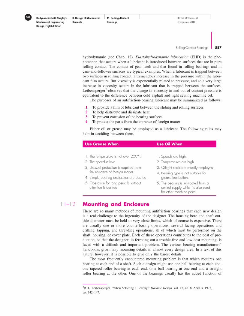
Budynas−Nisbett: Shigley’s
Mechanical Engineering
Design, Eighth Edition
III. Design of Mechanical
Elements
11. Rolling−Contact
Bearings
588 © The McGraw−Hill
Companies, 2008
Rolling-Contact Bearings 587
2R. L. Leibensperger, “When Selecting a Bearing,” Machine Design, vol. 47, no. 8, April 3, 1975,
pp. 142–147.
hydrodynamic (see Chap. 12). Elastohydrodynamic lubrication (EHD) is the phe-
nomenon that occurs when a lubricant is introduced between surfaces that are in pure
rolling contact. The contact of gear teeth and that found in rolling bearings and in
cam-and-follower surfaces are typical examples. When a lubricant is trapped between
two surfaces in rolling contact, a tremendous increase in the pressure within the lubri-
cant film occurs. But viscosity is exponentially related to pressure, and so a very large
increase in viscosity occurs in the lubricant that is trapped between the surfaces.
Leibensperger2 observes that the change in viscosity in and out of contact pressure is
equivalent to the difference between cold asphalt and light sewing machine oil.
The purposes of an antifriction-bearing lubricant may be summarized as follows:
1 To provide a film of lubricant between the sliding and rolling surfaces
2 To help distribute and dissipate heat
3 To prevent corrosion of the bearing surfaces
4 To protect the parts from the entrance of foreign matter
Either oil or grease may be employed as a lubricant. The following rules may
help in deciding between them.
11–12 Mounting and EnclosureThere are so many methods of mounting antifriction bearings that each new design
is a real challenge to the ingenuity of the designer. The housing bore and shaft out-
side diameter must be held to very close limits, which of course is expensive. There
are usually one or more counterboring operations, several facing operations and
drilling, tapping, and threading operations, all of which must be performed on the
shaft, housing, or cover plate. Each of these operations contributes to the cost of pro-
duction, so that the designer, in ferreting out a trouble-free and low-cost mounting, is
faced with a difficult and important problem. The various bearing manufacturers’
handbooks give many mounting details in almost every design area. In a text of this
nature, however, it is possible to give only the barest details.
The most frequently encountered mounting problem is that which requires one
bearing at each end of a shaft. Such a design might use one ball bearing at each end,
one tapered roller bearing at each end, or a ball bearing at one end and a straight
roller bearing at the other. One of the bearings usually has the added function of
Use Grease When Use Oil When
1. The temperature is not over 200°F.
2. The speed is low.
3. Unusual protection is required fromthe entrance of foreign matter.
4. Simple bearing enclosures are desired.
5. Operation for long periods withoutattention is desired.
1. Speeds are high.
2. Temperatures are high.
3. Oiltight seals are readily employed.
4. Bearing type is not suitable forgrease lubrication.
5. The bearing is lubricated from acentral supply which is also usedfor other machine parts.
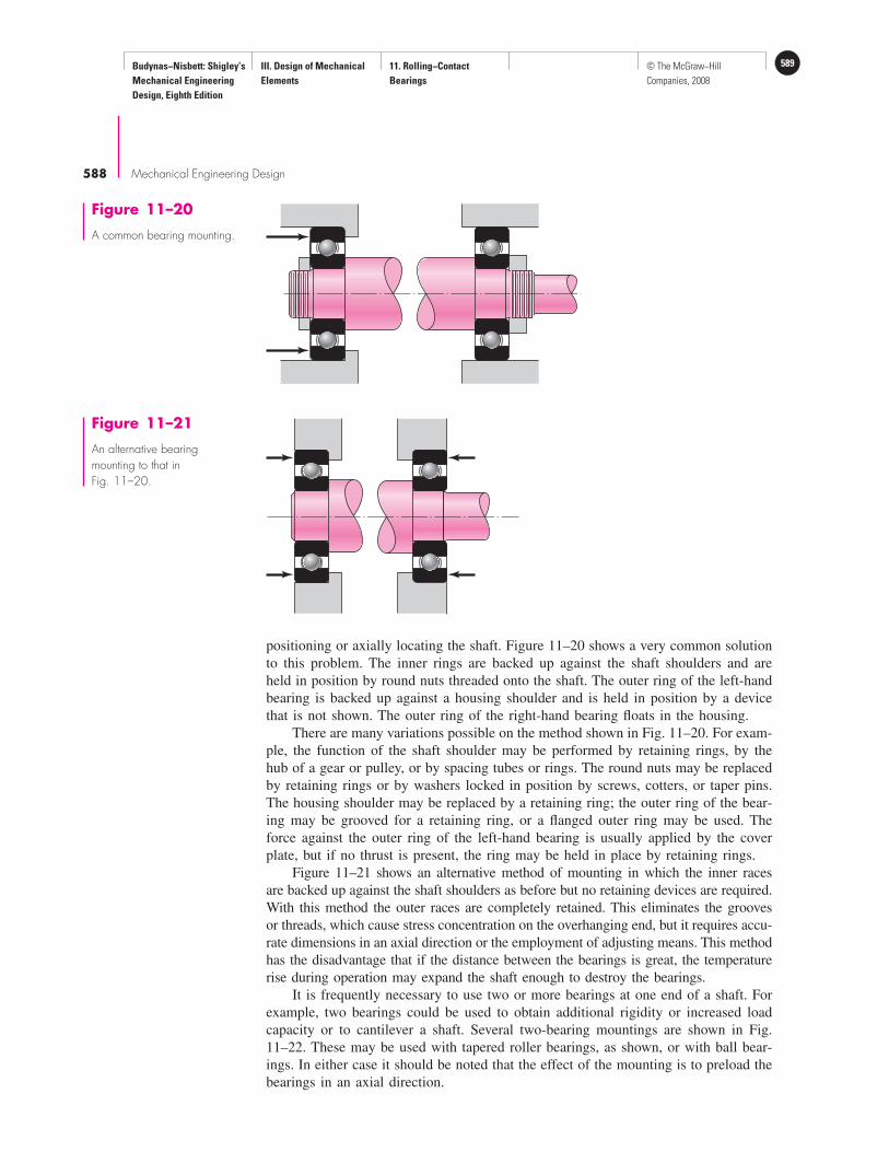
Budynas−Nisbett: Shigley’s
Mechanical Engineering
Design, Eighth Edition
III. Design of Mechanical
Elements
11. Rolling−Contact
Bearings
589© The McGraw−Hill
Companies, 2008
588 Mechanical Engineering Design
positioning or axially locating the shaft. Figure 11–20 shows a very common solution
to this problem. The inner rings are backed up against the shaft shoulders and are
held in position by round nuts threaded onto the shaft. The outer ring of the left-hand
bearing is backed up against a housing shoulder and is held in position by a device
that is not shown. The outer ring of the right-hand bearing floats in the housing.
There are many variations possible on the method shown in Fig. 11–20. For exam-
ple, the function of the shaft shoulder may be performed by retaining rings, by the
hub of a gear or pulley, or by spacing tubes or rings. The round nuts may be replaced
by retaining rings or by washers locked in position by screws, cotters, or taper pins.
The housing shoulder may be replaced by a retaining ring; the outer ring of the bear-
ing may be grooved for a retaining ring, or a flanged outer ring may be used. The
force against the outer ring of the left-hand bearing is usually applied by the cover
plate, but if no thrust is present, the ring may be held in place by retaining rings.
Figure 11–21 shows an alternative method of mounting in which the inner races
are backed up against the shaft shoulders as before but no retaining devices are required.
With this method the outer races are completely retained. This eliminates the grooves
or threads, which cause stress concentration on the overhanging end, but it requires accu-
rate dimensions in an axial direction or the employment of adjusting means. This method
has the disadvantage that if the distance between the bearings is great, the temperature
rise during operation may expand the shaft enough to destroy the bearings.
It is frequently necessary to use two or more bearings at one end of a shaft. For
example, two bearings could be used to obtain additional rigidity or increased load
capacity or to cantilever a shaft. Several two-bearing mountings are shown in Fig.
11–22. These may be used with tapered roller bearings, as shown, or with ball bear-
ings. In either case it should be noted that the effect of the mounting is to preload the
bearings in an axial direction.
Figure 11–20
A common bearing mounting.
Figure 11–21
An alternative bearingmounting to that inFig. 11–20.
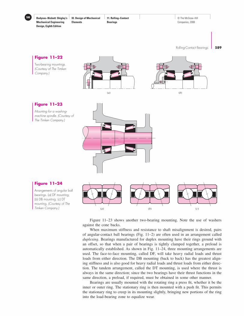
Budynas−Nisbett: Shigley’s
Mechanical Engineering
Design, Eighth Edition
III. Design of Mechanical
Elements
11. Rolling−Contact
Bearings
590 © The McGraw−Hill
Companies, 2008
Rolling-Contact Bearings 589
Figure 11–23 shows another two-bearing mounting. Note the use of washers
against the cone backs.
When maximum stiffness and resistance to shaft misalignment is desired, pairs
of angular-contact ball bearings (Fig. 11–2) are often used in an arrangement called
duplexing. Bearings manufactured for duplex mounting have their rings ground with
an offset, so that when a pair of bearings is tightly clamped together, a preload is
automatically established. As shown in Fig. 11–24, three mounting arrangements are
used. The face-to-face mounting, called DF, will take heavy radial loads and thrust
loads from either direction. The DB mounting (back to back) has the greatest align-
ing stiffness and is also good for heavy radial loads and thrust loads from either direc-
tion. The tandem arrangement, called the DT mounting, is used where the thrust is
always in the same direction; since the two bearings have their thrust functions in the
same direction, a preload, if required, must be obtained in some other manner.
Bearings are usually mounted with the rotating ring a press fit, whether it be the
inner or outer ring. The stationary ring is then mounted with a push fit. This permits
the stationary ring to creep in its mounting slightly, bringing new portions of the ring
into the load-bearing zone to equalize wear.
(a) (b)
Figure 11–22
Two-bearing mountings.(Courtesy of The TimkenCompany.)
Figure 11–23
Mounting for a washing-machine spindle. (Courtesy ofThe Timken Company.)
(a) (b) (c)
Figure 11–24
Arrangements of angular ballbearings. (a) DF mounting;(b) DB mounting; (c) DTmounting. (Courtesy of TheTimken Company.)

Budynas−Nisbett: Shigley’s
Mechanical Engineering
Design, Eighth Edition
III. Design of Mechanical
Elements
11. Rolling−Contact
Bearings
591© The McGraw−Hill
Companies, 2008
590 Mechanical Engineering Design
Preloading
The object of preloading is to remove the internal clearance usually found in bear-
ings, to increase the fatigue life, and to decrease the shaft slope at the bearing. Fig-
ure 11–25 shows a typical bearing in which the clearance is exaggerated for clarity.
Preloading of straight roller bearings may be obtained by:
1 Mounting the bearing on a tapered shaft or sleeve to expand the inner ring
2 Using an interference fit for the outer ring
3 Purchasing a bearing with the outer ring preshrunk over the rollers
Ball bearings are usually preloaded by the axial load built in during assembly.
However, the bearings of Fig. 11–24a and b are preloaded in assembly because of the
differences in widths of the inner and outer rings.
It is always good practice to follow manufacturers’ recommendations in deter-
mining preload, since too much will lead to early failure.
Alignment
Based on the general experience with rolling bearings as expressed in manufacturers’
catalogs, the permissible misalignment in cylindrical and tapered roller bearings is
limited to 0.001 rad. For spherical ball bearings, the misalignment should not exceed
0.0087 rad. But for deep-groove ball bearings, the allowable range of misalignment
is 0.0035 to 0.0047 rad. The life of the bearing decreases significantly when the mis-
alignment exceeds the allowable limits.
Additional protection against misalignment is obtained by providing the full
shoulders (see Fig. 11–8) recommended by the manufacturer. Also, if there is any mis-
alignment at all, it is good practice to provide a safety factor of around 2 to account
for possible increases during assembly.
Enclosures
To exclude dirt and foreign matter and to retain the lubricant, the bearing mountings
must include a seal. The three principal methods of sealings are the felt seal, the com-
mercial seal, and the labyrinth seal (Fig. 11–26).
Felt seals may be used with grease lubrication when the speeds are low. The rub-
bing surfaces should have a high polish. Felt seals should be protected from dirt by
placing them in machined grooves or by using metal stampings as shields.
The commercial seal is an assembly consisting of the rubbing element and, gen-
erally, a spring backing, which are retained in a sheet-metal jacket. These seals are
usually made by press fitting them into a counterbored hole in the bearing cover. Since
they obtain the sealing action by rubbing, they should not be used for high speeds.
The labyrinth seal is especially effective for high-speed installations and may be used
with either oil or grease. It is sometimes used with flingers. At least three grooves should
Clearance
Figure 11–25
Clearance in an off-the-shelfbearing, exaggerated forclarity.
(a) Felt seal (b) Commercial seal (c) Labyrinth seal
Figure 11–26
Typical sealing methods.(General Motors Corp. Usedwith permission, GM MediaArchives.)
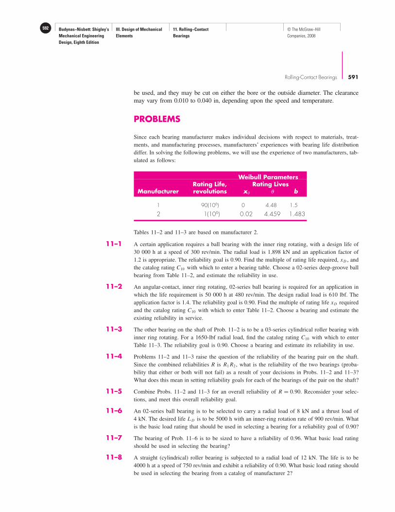
Budynas−Nisbett: Shigley’s
Mechanical Engineering
Design, Eighth Edition
III. Design of Mechanical
Elements
11. Rolling−Contact
Bearings
592 © The McGraw−Hill
Companies, 2008
Rolling-Contact Bearings 591
be used, and they may be cut on either the bore or the outside diameter. The clearance
may vary from 0.010 to 0.040 in, depending upon the speed and temperature.
PROBLEMS
Since each bearing manufacturer makes individual decisions with respect to materials, treat-
ments, and manufacturing processes, manufacturers’ experiences with bearing life distribution
differ. In solving the following problems, we will use the experience of two manufacturers, tab-
ulated as follows:
Tables 11–2 and 11–3 are based on manufacturer 2.
11–1 A certain application requires a ball bearing with the inner ring rotating, with a design life of
30 000 h at a speed of 300 rev/min. The radial load is 1.898 kN and an application factor of
1.2 is appropriate. The reliability goal is 0.90. Find the multiple of rating life required, xD , and
the catalog rating C10 with which to enter a bearing table. Choose a 02-series deep-groove ball
bearing from Table 11–2, and estimate the reliability in use.
11–2 An angular-contact, inner ring rotating, 02-series ball bearing is required for an application in
which the life requirement is 50 000 h at 480 rev/min. The design radial load is 610 lbf. The
application factor is 1.4. The reliability goal is 0.90. Find the multiple of rating life xD required
and the catalog rating C10 with which to enter Table 11–2. Choose a bearing and estimate the
existing reliability in service.
11–3 The other bearing on the shaft of Prob. 11–2 is to be a 03-series cylindrical roller bearing with
inner ring rotating. For a 1650-lbf radial load, find the catalog rating C10 with which to enter
Table 11–3. The reliability goal is 0.90. Choose a bearing and estimate its reliability in use.
11–4 Problems 11–2 and 11–3 raise the question of the reliability of the bearing pair on the shaft.
Since the combined reliabilities R is R1 R2 , what is the reliability of the two bearings (proba-
bility that either or both will not fail) as a result of your decisions in Probs. 11–2 and 11–3?
What does this mean in setting reliability goals for each of the bearings of the pair on the shaft?
11–5 Combine Probs. 11–2 and 11–3 for an overall reliability of R = 0.90. Reconsider your selec-
tions, and meet this overall reliability goal.
11–6 An 02-series ball bearing is to be selected to carry a radial load of 8 kN and a thrust load of
4 kN. The desired life L D is to be 5000 h with an inner-ring rotation rate of 900 rev/min. What
is the basic load rating that should be used in selecting a bearing for a reliability goal of 0.90?
11–7 The bearing of Prob. 11–6 is to be sized to have a reliability of 0.96. What basic load rating
should be used in selecting the bearing?
11–8 A straight (cylindrical) roller bearing is subjected to a radial load of 12 kN. The life is to be
4000 h at a speed of 750 rev/min and exhibit a reliability of 0.90. What basic load rating should
be used in selecting the bearing from a catalog of manufacturer 2?
Weibull ParametersRating Life, Rating Lives
Manufacturer revolutions x0 � b
1 90(106) 0 4.48 1.5
2 1(106) 0.02 4.459 1.483

Budynas−Nisbett: Shigley’s
Mechanical Engineering
Design, Eighth Edition
III. Design of Mechanical
Elements
11. Rolling−Contact
Bearings
593© The McGraw−Hill
Companies, 2008
592 Mechanical Engineering Design
11–9 Shown in the figure is a gear-driven squeeze roll that mates with an idler roll, below. The roll is
designed to exert a normal force of 30 lbf/in of roll length and a pull of 24 lbf/in on the material
being processed. The roll speed is 300 rev/min, and a design life of 30 000 h is desired. Use an
application factor of 1.2, and select a pair of angular-contact 02-series ball bearings from Table
11–2 to be mounted at 0 and A. Use the same size bearings at both locations and a combined reli-
ability of at least 0.92.
Gear 4
3 dia.
x
F
B
A
y
O
z 20°
4 dia.
1
8
2
3
2
3
4
13
4
3
4
Problem 11–9
Idler roll is below powered roll.Dimensions in inches.
z
20
16
10
20°
OFC
FA
AA
y
x
Gear 3
24 dia.
Gear 4
10 dia.
20°
B
C 2C
Problem 11–10
Dimensions in inches.
11–10 The figure shown is a geared countershaft with an overhanging pinion at C. Select an angular-
contact ball bearing from Table 11–2 for mounting at O and a straight roller bearing for mount-
ing at B. The force on gear A is FA = 600 lbf, and the shaft is to run at a speed of 480 rev/min.
Solution of the statics problem gives force of bearings against the shaft at O as
RO = −387j + 467k lbf, and at B as RB = 316j − 1615k lbf. Specify the bearings required, using
an application factor of 1.4, a desired life of 50 000 h, and a combined reliability goal of 0.90.
11–11 The figure is a schematic drawing of a countershaft that supports two V-belt pulleys. The coun-
tershaft runs at 1200 rev/min and the bearings are to have a life of 60 kh at a combined reli-
ability of 0.999. The belt tension on the loose side of pulley A is 15 percent of the tension on
the tight side. Select deep-groove bearings from Table 11–2 for use at O and E, each to have
a 25-mm bore, using an application factor of unity.

Budynas−Nisbett: Shigley’s
Mechanical Engineering
Design, Eighth Edition
III. Design of Mechanical
Elements
11. Rolling−Contact
Bearings
594 © The McGraw−Hill
Companies, 2008
Rolling-Contact Bearings 593
11–12 The bearing lubricant (513 SUS at 100◦F) operating point is 135◦F. A countershaft is supported
by two tapered roller bearings using an indirect mounting. The radial bearing loads are 560 lbf
for the left-hand bearing and 1095 for the right-hand bearing. The shaft rotates at 400 rev/min
and is to have a desired life of 40 kh. Use an application factor of 1.4 and a combined relia-
bility goal of 0.90. Using an initial K = 1.5, find the required radial rating for each bearing.
Select the bearings from Fig. 11–15.
11–13 A gear-reduction unit uses the countershaft depicted in the figure. Find the two bearing reac-
tions. The bearings are to be angular-contact ball bearings, having a desired life of 40 kh when
used at 200 rev/min. Use 1.2 for the application factor and a reliability goal for the bearing
pair of 0.95. Select the bearings from Table 11–2.
11–14 The worm shaft shown in part a of the figure transmits 1.35 hp at 600 rev/min. A static force
analysis gave the results shown in part b of the figure. Bearing A is to be an angular-contact
ball bearing mounted to take the 555-lbf thrust load. The bearing at B is to take only the radial
load, so a straight roller bearing will be employed. Use an application factor of 1.3, a desired
life of 25 kh, and a reliability goal, combined, of 0.99. Specify each bearing.
270 N
z
300
400
150
O
y
250 dia.
A
B
45°
P2P1
50 N
4
C
D
E
300 dia.
x
3
2Problem 11–11
Dimensions in millimeters.
z
16
14
O
B C
y
20°
240 lbf
Gear 3, 24 dia.
x
2
12
F
25°
Gear 4, 12 dia.
A
Problem 11–13
Dimensions in inches.
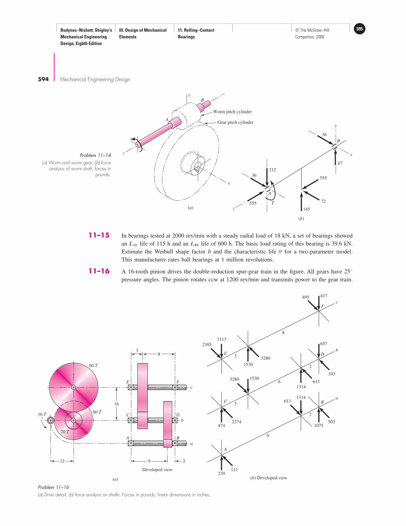
Budynas−Nisbett: Shigley’s
Mechanical Engineering
Design, Eighth Edition
III. Design of Mechanical
Elements
11. Rolling−Contact
Bearings
595© The McGraw−Hill
Companies, 2008
594 Mechanical Engineering Design
(a)
38
912 2
60 T
E
C
A
F
c
b
a
D
B
20 T
16 T80 T
16
Developed view
Problem 11–16
(a) Drive detail; (b) force analysis on shafts. Forces in pounds; linear dimensions in inches.
(b) Developed view
2385
1113
1530
3280E
8
3
895 417
Fc
8742274
3280 1530
C
6
2
3613
1314
393
6131314
657
Db
239111
A
9
2
1075502
Ba
z
A
yB
z
x
A
T555
36
212
145
67
36
y
x
B
72
555
Worm pitch cylinder
Gear pitch cylinder
(a)
(b)
Problem 11–14
(a) Worm and worm gear; (b) forceanalysis of worm shaft, forces in
pounds.
11–15 In bearings tested at 2000 rev/min with a steady radial load of 18 kN, a set of bearings showed
an L10 life of 115 h and an L80 life of 600 h. The basic load rating of this bearing is 39.6 kN.
Estimate the Weibull shape factor b and the characteristic life θ for a two-parameter model.
This manufacturer rates ball bearings at 1 million revolutions.
11–16 A 16-tooth pinion drives the double-reduction spur-gear train in the figure. All gears have 25◦
pressure angles. The pinion rotates ccw at 1200 rev/min and transmits power to the gear train.

Budynas−Nisbett: Shigley’s
Mechanical Engineering
Design, Eighth Edition
III. Design of Mechanical
Elements
11. Rolling−Contact
Bearings
596 © The McGraw−Hill
Companies, 2008
Rolling-Contact Bearings 595
The shaft has not yet been designed, but the free bodies have been generated. The shaft speeds
are 1200 rev/min, 240 rev/min, and 80 rev/min. A bearing study is commencing with a 10-kh
life and a gearbox bearing ensemble reliability of 0.99. An application factor of 1.2 is appro-
priate. Specify the six bearings.
11–17 Different bearing metallurgy affects bearing life. A manufacturer reports that a particular heat
treatment increases bearing life at least threefold. A bearing identical to that of Prob. 11–15
except for the heat treatment, loaded to 18 kN and run at 2000 rev/min, revealed an L10 life
of 360 h and an L80 life of 2000 h. Do you agree with the manufacturer's assertion concern-
ing increased life?
11–18 Estimate the remaining life in revolutions of an 02-30 mm angular-contact ball bearing already
subjected to 200 000 revolutions with a radial load of 18 kN, if it is now to be subjected to a
change in load to 30 kN.
11–19 The same 02-30 angular-contact ball bearing as in Prob. 11–18 is to be subjected to a two-step
loading cycle of 4 min with a loading of 18 kN, and one of 6 min with a loading of 30 kN. This
cycle is to be repeated until failure. Estimate the total life in revolutions, hours, and loading
cycles.
11–20 The expression Fa L = constant can be written using x = L/L10 , and it can be expressed as
Fa x = K or log F = (1/a) log K − (1/a) log x . This is a straight line on a log-log plot, and
it is the basis of Fig. 11–5. For the geometric insight provided, produce Fig. 11–5 to scale using
Ex. 11–3, and
For point D: find FD = 1.2(413) = 495.6 lbf, log FD , xD , log xD , K D
For point B: find xB , log xB , FB , log FB , K B
For point A: find FA = FB = C10 , log FA , K10
and plot to scale. On this plot, also show the line containing C10 , the basic load rating, of the
selected bearing.

Budynas−Nisbett: Shigley’s
Mechanical Engineering
Design, Eighth Edition
III. Design of Mechanical
Elements
12. Lubrication and Journal
Bearings
597© The McGraw−Hill
Companies, 2008
Lubrication and JournalBearings
Chapter Outline
12–1 Types of Lubrication 598
12–2 Viscosity 599
12–3 Petroff’s Equation 601
12–4 Stable Lubrication 603
12–5 Thick-Film Lubrication 604
12–6 Hydrodynamic Theory 605
12–7 Design Considerations 609
12–8 The Relations of the Variables 611
12–9 Steady-State Conditions in Self-Contained Bearings 625
12–10 Clearance 628
12–11 Pressure-Fed Bearings 630
12–12 Loads and Materials 636
12–13 Bearing Types 638
12–14 Thrust Bearings 639
12–15 Boundary-Lubricated Bearings 640
12
597

Budynas−Nisbett: Shigley’s
Mechanical Engineering
Design, Eighth Edition
III. Design of Mechanical
Elements
12. Lubrication and Journal
Bearings
598 © The McGraw−Hill
Companies, 2008
598 Mechanical Engineering Design
The object of lubrication is to reduce friction, wear, and heating of machine parts that
move relative to each other. A lubricant is any substance that, when inserted between
the moving surfaces, accomplishes these purposes. In a sleeve bearing, a shaft, or jour-
nal, rotates or oscillates within a sleeve, or bushing, and the relative motion is sliding.
In an antifriction bearing, the main relative motion is rolling. A follower may either roll
or slide on the cam. Gear teeth mate with each other by a combination of rolling and
sliding. Pistons slide within their cylinders. All these applications require lubrication to
reduce friction, wear, and heating.
The field of application for journal bearings is immense. The crankshaft and
connecting-rod bearings of an automotive engine must operate for thousands of miles at
high temperatures and under varying load conditions. The journal bearings used in the
steam turbines of power-generating stations are said to have reliabilities approaching
100 percent. At the other extreme there are thousands of applications in which the
loads are light and the service relatively unimportant; a simple, easily installed bearing
is required, using little or no lubrication. In such cases an antifriction bearing might be a
poor answer because of the cost, the elaborate enclosures, the close tolerances, the radial
space required, the high speeds, or the increased inertial effects. Instead, a nylon bearing
requiring no lubrication, a powder-metallurgy bearing with the lubrication “built in,” or
a bronze bearing with ring oiling, wick feeding, or solid-lubricant film or grease lubri-
cation might be a very satisfactory solution. Recent metallurgy developments in bearing
materials, combined with increased knowledge of the lubrication process, now make it
possible to design journal bearings with satisfactory lives and very good reliabilities.
Much of the material we have studied thus far in this book has been based on fun-
damental engineering studies, such as statics, dynamics, the mechanics of solids, metal
processing, mathematics, and metallurgy. In the study of lubrication and journal bear-
ings, additional fundamental studies, such as chemistry, fluid mechanics, thermody-
namics, and heat transfer, must be utilized in developing the material. While we shall
not utilize all of them in the material to be included here, you can now begin to appre-
ciate better how the study of mechanical engineering design is really an integration
of most of your previous studies and a directing of this total background toward the
resolution of a single objective.
12–1 Types of LubricationFive distinct forms of lubrication may be identified:
1 Hydrodynamic
2 Hydrostatic
3 Elastohydrodynamic
4 Boundary
5 Solid film
Hydrodynamic lubrication means that the load-carrying surfaces of the bearing are
separated by a relatively thick film of lubricant, so as to prevent metal-to-metal contact,
and that the stability thus obtained can be explained by the laws of fluid mechanics.
Hydrodynamic lubrication does not depend upon the introduction of the lubricant under
pressure, though that may occur; but it does require the existence of an adequate sup-
ply at all times. The film pressure is created by the moving surface itself pulling the
lubricant into a wedge-shaped zone at a velocity sufficiently high to create the pressure
necessary to separate the surfaces against the load on the bearing. Hydrodynamic lubri-
cation is also called full-film, or fluid, lubrication.
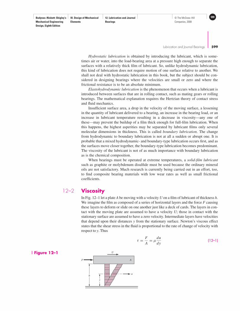
Budynas−Nisbett: Shigley’s
Mechanical Engineering
Design, Eighth Edition
III. Design of Mechanical
Elements
12. Lubrication and Journal
Bearings
599© The McGraw−Hill
Companies, 2008
Lubrication and Journal Bearings 599
Figure 12–1
F
uh
y
U
A
Hydrostatic lubrication is obtained by introducing the lubricant, which is some-
times air or water, into the load-bearing area at a pressure high enough to separate the
surfaces with a relatively thick film of lubricant. So, unlike hydrodynamic lubrication,
this kind of lubrication does not require motion of one surface relative to another. We
shall not deal with hydrostatic lubrication in this book, but the subject should be con-
sidered in designing bearings where the velocities are small or zero and where the
frictional resistance is to be an absolute minimum.
Elastohydrodynamic lubrication is the phenomenon that occurs when a lubricant is
introduced between surfaces that are in rolling contact, such as mating gears or rolling
bearings. The mathematical explanation requires the Hertzian theory of contact stress
and fluid mechanics.
Insufficient surface area, a drop in the velocity of the moving surface, a lessening
in the quantity of lubricant delivered to a bearing, an increase in the bearing load, or an
increase in lubricant temperature resulting in a decrease in viscosity—any one of
these—may prevent the buildup of a film thick enough for full-film lubrication. When
this happens, the highest asperities may be separated by lubricant films only several
molecular dimensions in thickness. This is called boundary lubrication. The change
from hydrodynamic to boundary lubrication is not at all a sudden or abrupt one. It is
probable that a mixed hydrodynamic- and boundary-type lubrication occurs first, and as
the surfaces move closer together, the boundary-type lubrication becomes predominant.
The viscosity of the lubricant is not of as much importance with boundary lubrication
as is the chemical composition.
When bearings must be operated at extreme temperatures, a solid-film lubricant
such as graphite or molybdenum disulfide must be used because the ordinary mineral
oils are not satisfactory. Much research is currently being carried out in an effort, too,
to find composite bearing materials with low wear rates as well as small frictional
coefficients.
12–2 ViscosityIn Fig. 12–1 let a plate A be moving with a velocity U on a film of lubricant of thickness h.
We imagine the film as composed of a series of horizontal layers and the force F causing
these layers to deform or slide on one another just like a deck of cards. The layers in con-
tact with the moving plate are assumed to have a velocity U; those in contact with the
stationary surface are assumed to have a zero velocity. Intermediate layers have velocities
that depend upon their distances y from the stationary surface. Newton’s viscous effect
states that the shear stress in the fluid is proportional to the rate of change of velocity with
respect to y. Thus
τ = F
A= µ
du
dy(12–1)

Budynas−Nisbett: Shigley’s
Mechanical Engineering
Design, Eighth Edition
III. Design of Mechanical
Elements
12. Lubrication and Journal
Bearings
600 © The McGraw−Hill
Companies, 2008
600 Mechanical Engineering Design
where µ is the constant of proportionality and defines absolute viscosity, also called
dynamic viscosity. The derivative du/dy is the rate of change of velocity with distance
and may be called the rate of shear, or the velocity gradient. The viscosity µ is thus a
measure of the internal frictional resistance of the fluid. For most lubricating fluids, the
rate of shear is constant, and du/dy = U/h . Thus, from Eq. (12–1),
τ = F
A= µ
U
h(12–2)
Fluids exhibiting this characteristic are said to be Newtonian fluids. The unit of vis-
cosity in the ips system is seen to be the pound-force-second per square inch; this is the
same as stress or pressure multiplied by time. The ips unit is called the reyn, in honor
of Sir Osborne Reynolds.
The absolute viscosity is measured by the pascal-second (Pa · s) in SI; this is the
same as a Newton-second per square meter. The conversion from ips units to SI is the
same as for stress. For example, multiply the absolute viscosity in reyns by 6890 to
convert to units of Pa · s.
The American Society of Mechanical Engineers (ASME) has published a list of
cgs units that are not to be used in ASME documents.1 This list results from a recom-
mendation by the International Committee of Weights and Measures (CIPM) that the
use of cgs units with special names be discouraged. Included in this list is a unit of force
called the dyne (dyn), a unit of dynamic viscosity called the poise (P), and a unit of
kinematic viscosity called the stoke (St). All of these units have been, and still are, used
extensively in lubrication studies.
The poise is the cgs unit of dynamic or absolute viscosity, and its unit is the dyne-
second per square centimeter (dyn · s/cm2). It has been customary to use the centipoise
(cP) in analysis, because its value is more convenient. When the viscosity is expressed in
centipoises, it is designated by Z. The conversion from cgs units to SI and ips units is as
follows:
µ(Pa · s) = (10)−3 Z (cP)
µ(reyn) = Z (cP)
6.89(10)6
µ(mPa · s) = 6.89 µ′(µreyn)
In using ips units, the microreyn (µreyn) is often more convenient. The symbol µ′ will
be used to designate viscosity in µreyn such that µ = µ′/(106).
The ASTM standard method for determining viscosity uses an instrument called the
Saybolt Universal Viscosimeter. The method consists of measuring the time in seconds
for 60 mL of lubricant at a specified temperature to run through a tube 17.6 mm in
diameter and 12.25 mm long. The result is called the kinematic viscosity, and in the past
the unit of the square centimeter per second has been used. One square centimeter per sec-
ond is defined as a stoke. By the use of the Hagen-Poiseuille law, the kinematic viscosity
based upon seconds Saybolt, also called Saybolt Universal viscosity (SUV) in seconds, is
Zk =(
0.22t − 180
t
)
(12–3)
where Zk is in centistokes (cSt) and t is the number of seconds Saybolt.
1ASME Orientation and Guide for Use of Metric Units, 2nd ed., American Society of Mechanical Engineers,
1972, p. 13.
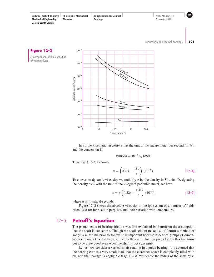
Budynas−Nisbett: Shigley’s
Mechanical Engineering
Design, Eighth Edition
III. Design of Mechanical
Elements
12. Lubrication and Journal
Bearings
601© The McGraw−Hill
Companies, 2008
Lubrication and Journal Bearings 601
Figure 12–2
A comparison of the viscositiesof various fluids.
Air
0 50 100 150 20010−9
10−8
10−7
10−6
10−5
10−4
10−3
Temperature, °F
Abso
lute
vis
cosi
ty, re
yn
Castor oilSAE 30 oil
Water
Gasoline
In SI, the kinematic viscosity ν has the unit of the square meter per second (m2/s),
and the conversion is
ν(m2/s) = 10−6 Zk (cSt)
Thus, Eq. (12–3) becomes
ν =(
0.22t − 180
t
)
(10−6) (12–4)
To convert to dynamic viscosity, we multiply ν by the density in SI units. Designating
the density as ρ with the unit of the kilogram per cubic meter, we have
µ = ρ
(
0.22t − 180
t
)
(10−6) (12–5)
where µ is in pascal-seconds.
Figure 12–2 shows the absolute viscosity in the ips system of a number of fluids
often used for lubrication purposes and their variation with temperature.
12–3 Petroff’s EquationThe phenomenon of bearing friction was first explained by Petroff on the assumption
that the shaft is concentric. Though we shall seldom make use of Petroff’s method of
analysis in the material to follow, it is important because it defines groups of dimen-
sionless parameters and because the coefficient of friction predicted by this law turns
out to be quite good even when the shaft is not concentric.
Let us now consider a vertical shaft rotating in a guide bearing. It is assumed that
the bearing carries a very small load, that the clearance space is completely filled with
oil, and that leakage is negligible (Fig. 12–3). We denote the radius of the shaft by r,

Budynas−Nisbett: Shigley’s
Mechanical Engineering
Design, Eighth Edition
III. Design of Mechanical
Elements
12. Lubrication and Journal
Bearings
602 © The McGraw−Hill
Companies, 2008
602 Mechanical Engineering Design
Figure 12–3
Petroff’s lightly loaded journalbearing consisting of a shaftjournal and a bushing with anaxial-groove internal lubricantreservoir. The linear velocitygradient is shown in the endview. The clearance c isseveral thousandths of an inchand is grossly exaggerated forpresentation purposes.
A
N
A'
W W
r
c W
l
Section AA'
W
U
“Keyway”
sump
Oilfill
hole
Bushing (bearing)
Journal (shaft)
Side leakage negligible
the radial clearance by c, and the length of the bearing by l, all dimensions being in
inches. If the shaft rotates at N rev/s, then its surface velocity is U = 2πr N in/s. Since
the shearing stress in the lubricant is equal to the velocity gradient times the viscosity,
from Eq. (12–2) we have
τ = µU
h= 2πrµN
c(a)
where the radial clearance c has been substituted for the distance h. The force required
to shear the film is the stress times the area. The torque is the force times the lever arm
r. Thus
T = (τ A)(r) =(
2πrµN
c
)
(2πrl)(r) = 4π2r3lµN
c(b)
If we now designate a small force on the bearing by W, in pounds-force, then the pres-
sure P, in pounds-force per square inch of projected area, is P = W/2rl . The frictional
force is f W , where f is the coefficient of friction, and so the frictional torque is
T = f Wr = ( f )(2rl P)(r) = 2r2 f l P (c)
Substituting the value of the torque from Eq. (c) in Eq. (b) and solving for the coeffi-
cient of friction, we find
f = 2π2 µN
P
r
c(12–6)
Equation (12–6) is called Petroff’s equation and was first published in 1883. The
two quantities µN/P and r/c are very important parameters in lubrication. Substitution
of the appropriate dimensions in each parameter will show that they are dimensionless.
The bearing characteristic number, or the Sommerfeld number, is defined by the
equation
S =(
r
c
)2µN
P(12–7)
The Sommerfeld number is very important in lubrication analysis because it contains
many of the parameters that are specified by the designer. Note that it is also dimen-
sionless. The quantity r/c is called the radial clearance ratio. If we multiply both sides
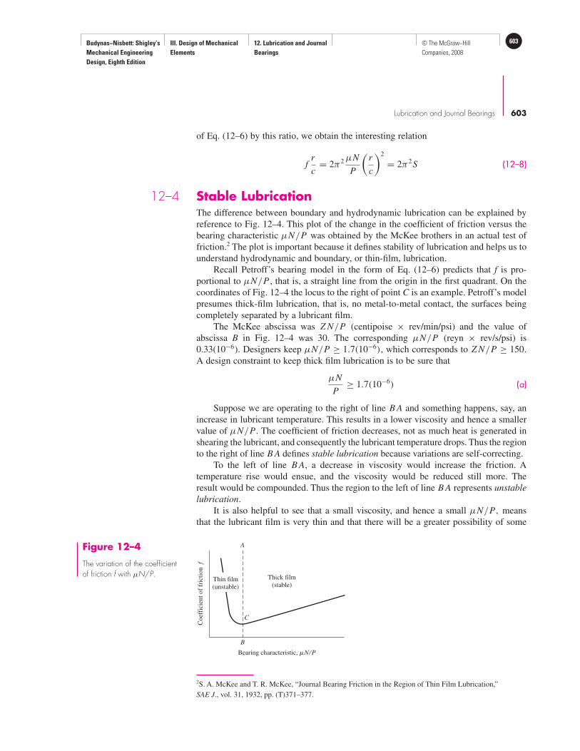
Budynas−Nisbett: Shigley’s
Mechanical Engineering
Design, Eighth Edition
III. Design of Mechanical
Elements
12. Lubrication and Journal
Bearings
603© The McGraw−Hill
Companies, 2008
Lubrication and Journal Bearings 603
of Eq. (12–6) by this ratio, we obtain the interesting relation
fr
c= 2π2 µN
P
(
r
c
)2
= 2π2S (12–8)
12–4 Stable LubricationThe difference between boundary and hydrodynamic lubrication can be explained by
reference to Fig. 12–4. This plot of the change in the coefficient of friction versus the
bearing characteristic µN/P was obtained by the McKee brothers in an actual test of
friction.2 The plot is important because it defines stability of lubrication and helps us to
understand hydrodynamic and boundary, or thin-film, lubrication.
Recall Petroff’s bearing model in the form of Eq. (12–6) predicts that f is pro-
portional to µN/P , that is, a straight line from the origin in the first quadrant. On the
coordinates of Fig. 12–4 the locus to the right of point C is an example. Petroff’s model
presumes thick-film lubrication, that is, no metal-to-metal contact, the surfaces being
completely separated by a lubricant film.
The McKee abscissa was Z N/P (centipoise × rev/min/psi) and the value of
abscissa B in Fig. 12–4 was 30. The corresponding µN/P (reyn × rev/s/psi) is
0.33(10−6). Designers keep µN/P ≥ 1.7(10−6), which corresponds to Z N/P ≥ 150.
A design constraint to keep thick film lubrication is to be sure that
µN
P≥ 1.7(10−6) (a)
Suppose we are operating to the right of line B A and something happens, say, an
increase in lubricant temperature. This results in a lower viscosity and hence a smaller
value of µN/P. The coefficient of friction decreases, not as much heat is generated in
shearing the lubricant, and consequently the lubricant temperature drops. Thus the region
to the right of line B A defines stable lubrication because variations are self-correcting.
To the left of line B A, a decrease in viscosity would increase the friction. A
temperature rise would ensue, and the viscosity would be reduced still more. The
result would be compounded. Thus the region to the left of line B A represents unstable
lubrication.
It is also helpful to see that a small viscosity, and hence a small µN/P, means
that the lubricant film is very thin and that there will be a greater possibility of some
Figure 12–4
The variation of the coefficientof friction f with µN/P.
B
A
C
Thick film
(stable)Thin film
(unstable)
Bearing characteristic, �N ⁄P
Coef
fici
ent
of
fric
tion f
2S. A. McKee and T. R. McKee, “Journal Bearing Friction in the Region of Thin Film Lubrication,”
SAE J., vol. 31, 1932, pp. (T)371–377.

Budynas−Nisbett: Shigley’s
Mechanical Engineering
Design, Eighth Edition
III. Design of Mechanical
Elements
12. Lubrication and Journal
Bearings
604 © The McGraw−Hill
Companies, 2008
604 Mechanical Engineering Design
Figure 12–5
Formation of a film.
W
Wh0
(a) Dry
W
Q (flow)
W
(b) Lubricated
metal-to-metal contact, and hence of more friction. Thus, point C represents what is
probably the beginning of metal-to-metal contact as µN/P becomes smaller.
12–5 Thick-Film LubricationLet us now examine the formation of a lubricant film in a journal bearing. Figure 12–5a
shows a journal that is just beginning to rotate in a clockwise direction. Under starting
conditions, the bearing will be dry, or at least partly dry, and hence the journal will
climb or roll up the right side of the bearing as shown in Fig. 12–5a.
Now suppose a lubricant is introduced into the top of the bearing as shown in
Fig. 12–5b. The action of the rotating journal is to pump the lubricant around the bear-
ing in a clockwise direction. The lubricant is pumped into a wedge-shaped space and
forces the journal over to the other side. A minimum film thickness h0 occurs, not at the
bottom of the journal, but displaced clockwise from the bottom as in Fig. 12–5b. This is
explained by the fact that a film pressure in the converging half of the film reaches a
maximum somewhere to the left of the bearing center.
Figure 12–5 shows how to decide whether the journal, under hydrodynamic lubrica-
tion, is eccentrically located on the right or on the left side of the bearing.Visualize the jour-
nal beginning to rotate. Find the side of the bearing upon which the journal tends to roll.
Then, if the lubrication is hydrodynamic, mentally place the journal on the opposite side.
The nomenclature of a journal bearing is shown in Fig. 12–6. The dimension c is
the radial clearance and is the difference in the radii of the bushing and journal. In
Figure 12–6
Nomenclature of a partialjournal bearing.
h0
O
eO'
N
r
Journal
Line of centers
Bushing
c = radial
clearance

Budynas−Nisbett: Shigley’s
Mechanical Engineering
Design, Eighth Edition
III. Design of Mechanical
Elements
12. Lubrication and Journal
Bearings
605© The McGraw−Hill
Companies, 2008
Lubrication and Journal Bearings 605
3Beauchamp Tower, “First Report on Friction Experiments,” Proc. Inst. Mech. Eng., November 1883,
pp. 632–666; “Second Report,” ibid., 1885, pp. 58–70; “Third Report,” ibid., 1888, pp. 173–205;
“Fourth Report,” ibid., 1891, pp. 111–140.
Fig. 12–6 the center of the journal is at O and the center of the bearing at O ′. The dis-
tance between these centers is the eccentricity and is denoted by e. The minimum film
thickness is designated by h0, and it occurs at the line of centers. The film thickness at
any other point is designated by h. We also define an eccentricity ratio ε as
ε = e
c
The bearing shown in the figure is known as a partial bearing. If the radius of the
bushing is the same as the radius of the journal, it is known as a fitted bearing. If the
bushing encloses the journal, as indicated by the dashed lines, it becomes a full bearing.
The angle β describes the angular length of a partial bearing. For example, a 120◦ partial
bearing has the angle β equal to 120◦.
12–6 Hydrodynamic TheoryThe present theory of hydrodynamic lubrication originated in the laboratory of
Beauchamp Tower in the early 1880s in England. Tower had been employed to study
the friction in railroad journal bearings and learn the best methods of lubricating them.
It was an accident or error, during the course of this investigation, that prompted Tower
to look at the problem in more detail and that resulted in a discovery that eventually led
to the development of the theory.
Figure 12–7 is a schematic drawing of the journal bearing that Tower investigated.
It is a partial bearing, having a diameter of 4 in, a length of 6 in, and a bearing arc of
157◦, and having bath-type lubrication, as shown. The coefficients of friction obtained
by Tower in his investigations on this bearing were quite low, which is now not
surprising. After testing this bearing, Tower later drilled a 12-in-diameter lubricator hole
through the top. But when the apparatus was set in motion, oil flowed out of this hole.
In an effort to prevent this, a cork stopper was used, but this popped out, and so it was
necessary to drive a wooden plug into the hole. When the wooden plug was pushed out
too, Tower, at this point, undoubtedly realized that he was on the verge of discovery. A
pressure gauge connected to the hole indicated a pressure of more than twice the unit
bearing load. Finally, he investigated the bearing film pressures in detail throughout the
bearing width and length and reported a distribution similar to that of Fig. 12–8.3
The results obtained by Tower had such regularity that Osborne Reynolds con-
cluded that there must be a definite equation relating the friction, the pressure, and the
Figure 12–7
Schematic representation ofthe partial bearing used byTower.
N
Journal
Lubricant
level
Lubricator holePartial bronze
bearingW

Budynas−Nisbett: Shigley’s
Mechanical Engineering
Design, Eighth Edition
III. Design of Mechanical
Elements
12. Lubrication and Journal
Bearings
606 © The McGraw−Hill
Companies, 2008
606 Mechanical Engineering Design
Figure 12–8
Approximate pressure-distribution curves obtainedby Tower.
pmax
p = 0
N
l = 6 in
d = 4 in
velocity. The present mathematical theory of lubrication is based upon Reynolds’ work
following the experiment by Tower.4 The original differential equation, developed by
Reynolds, was used by him to explain Tower’s results. The solution is a challenging
problem that has interested many investigators ever since then, and it is still the starting
point for lubrication studies.
Reynolds pictured the lubricant as adhering to both surfaces and being pulled by
the moving surface into a narrowing, wedge-shaped space so as to create a fluid or film
pressure of sufficient intensity to support the bearing load. One of the important sim-
plifying assumptions resulted from Reynolds’ realization that the fluid films were so
thin in comparison with the bearing radius that the curvature could be neglected. This
enabled him to replace the curved partial bearing with a flat bearing, called a plane slider
bearing. Other assumptions made were:
1 The lubricant obeys Newton’s viscous effect, Eq. (12–1).
2 The forces due to the inertia of the lubricant are neglected.
3 The lubricant is assumed to be incompressible.
4 The viscosity is assumed to be constant throughout the film.
5 The pressure does not vary in the axial direction.
Figure 12–9a shows a journal rotating in the clockwise direction supported by a
film of lubricant of variable thickness h on a partial bearing, which is fixed. We specify
that the journal has a constant surface velocity U. Using Reynolds’ assumption that
curvature can be neglected, we fix a right-handed xyz reference system to the stationary
bearing. We now make the following additional assumptions:
6 The bushing and journal extend infinitely in the z direction; this means there can
be no lubricant flow in the z direction.
7 The film pressure is constant in the y direction. Thus the pressure depends only
on the coordinate x.
8 The velocity of any particle of lubricant in the film depends only on the
coordinates x and y.
We now select an element of lubricant in the film (Fig. 12–9a) of dimensions dx ,
dy, and dz, and compute the forces that act on the sides of this element. As shown in
Fig. 12–9b, normal forces, due to the pressure, act upon the right and left sides of the
4Osborne Reynolds, “Theory of Lubrication, Part I,” Phil. Trans. Roy. Soc. London, 1886.

Budynas−Nisbett: Shigley’s
Mechanical Engineering
Design, Eighth Edition
III. Design of Mechanical
Elements
12. Lubrication and Journal
Bearings
607© The McGraw−Hill
Companies, 2008
Lubrication and Journal Bearings 607
dx
h
U
dy
Journal
(a) (b)
Partial bushing
dy
h
z
x
y
dx
� dx dz
p dy dz
∂y(� + dy) dx dz
∂�
dx(p + dx) dy dz
dp
u = U
Flow of
lubricant
Stationary partial bushing
Rotating journal
element, and shear forces, due to the viscosity and to the velocity, act upon the top and
bottom sides. Summing the forces in the x direction gives
∑
Fx = p dy dz −(
p + dp
dxdx
)
dy dz − τ dx dz +(
τ + ∂τ
∂ydy
)
dx dz = 0 (a)
This reduces to
dp
dx= ∂τ
∂y(b)
From Eq. (12–1), we have
τ = µ∂u
∂y(c)
where the partial derivative is used because the velocity u depends upon both x and y.
Substituting Eq. (c) in Eq. (b), we obtain
dp
dx= µ
∂2u
∂y2(d)
Holding x constant, we now integrate this expression twice with respect to y. This gives
∂u
∂y= 1
µ
dp
dxy + C1
u = 1
2µ
dp
dxy2 + C1 y + C2 (e)
Note that the act of holding x constant means that C1 and C2 can be functions of x. We
now assume that there is no slip between the lubricant and the boundary surfaces. This
gives two sets of boundary conditions for evaluating the constants C1 and C2:
At y = 0, u = 0
At y = h, u = U(f )
Figure 12–9

Budynas−Nisbett: Shigley’s
Mechanical Engineering
Design, Eighth Edition
III. Design of Mechanical
Elements
12. Lubrication and Journal
Bearings
608 © The McGraw−Hill
Companies, 2008
608 Mechanical Engineering Design
Notice, in the second condition, that h is a function of x. Substituting these conditions
in Eq. (e) and solving for the constants gives
C1 = U
h− h
2µ
dp
dxC2 = 0
or
u = 1
2µ
dp
dx(y2 − hy) + U
hy (12–9)
This equation gives the velocity distribution of the lubricant in the film as a function of
the coordinate y and the pressure gradient dp/dx . The equation shows that the velocity
distribution across the film (from y = 0 to y = h) is obtained by superposing a para-
bolic distribution onto a linear distribution. Figure 12–10 shows the superposition of
these distributions to obtain the velocity for particular values of x and dp/dx . In general,
the parabolic term may be additive or subtractive to the linear term, depending upon
the sign of the pressure gradient. When the pressure is maximum, dp/dx = 0 and the
velocity is
u = U
hy (g)
which is a linear relation.
We next define Q as the volume of lubricant flowing in the x direction per unit
time. By using a width of unity in the z direction, the volume may be obtained by the
expression
Q =∫ h
0
u dy (h)
Substituting the value of u from Eq. (12–9) and integrating gives
Q = Uh
2− h3
12µ
dp
dx(i )
The next step uses the assumption of an incompressible lubricant and states that the
flow is the same for any cross section. Thus
d Q
dx= 0
h
y
U
u
x
y
Flow of
lubricant
Stationary bushing
Rotating journal
dp
dx> 0
dp
dx= 0
dp
dx< 0
Figure 12–10
Velocity of the lubricant.
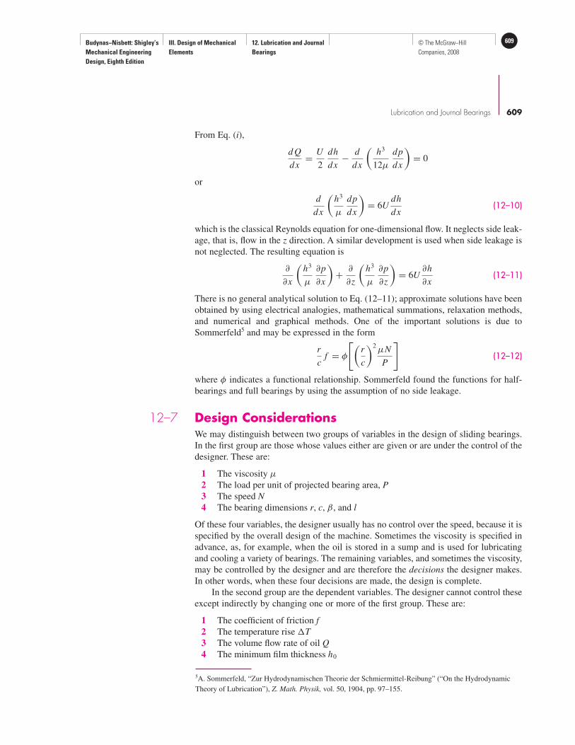
Budynas−Nisbett: Shigley’s
Mechanical Engineering
Design, Eighth Edition
III. Design of Mechanical
Elements
12. Lubrication and Journal
Bearings
609© The McGraw−Hill
Companies, 2008
Lubrication and Journal Bearings 609
From Eq. (i),
d Q
dx= U
2
dh
dx− d
dx
(
h3
12µ
dp
dx
)
= 0
or
d
dx
(
h3
µ
dp
dx
)
= 6Udh
dx(12–10)
which is the classical Reynolds equation for one-dimensional flow. It neglects side leak-
age, that is, flow in the z direction. A similar development is used when side leakage is
not neglected. The resulting equation is
∂
∂x
(
h3
µ
∂p
∂x
)
+ ∂
∂z
(
h3
µ
∂p
∂z
)
= 6U∂h
∂x(12–11)
There is no general analytical solution to Eq. (12–11); approximate solutions have been
obtained by using electrical analogies, mathematical summations, relaxation methods,
and numerical and graphical methods. One of the important solutions is due to
Sommerfeld5 and may be expressed in the form
r
cf = φ
[
(
r
c
)2µN
P
]
(12–12)
where φ indicates a functional relationship. Sommerfeld found the functions for half-
bearings and full bearings by using the assumption of no side leakage.
12–7 Design ConsiderationsWe may distinguish between two groups of variables in the design of sliding bearings.
In the first group are those whose values either are given or are under the control of the
designer. These are:
1 The viscosity µ
2 The load per unit of projected bearing area, P
3 The speed N
4 The bearing dimensions r, c, β , and l
Of these four variables, the designer usually has no control over the speed, because it is
specified by the overall design of the machine. Sometimes the viscosity is specified in
advance, as, for example, when the oil is stored in a sump and is used for lubricating
and cooling a variety of bearings. The remaining variables, and sometimes the viscosity,
may be controlled by the designer and are therefore the decisions the designer makes.
In other words, when these four decisions are made, the design is complete.
In the second group are the dependent variables. The designer cannot control these
except indirectly by changing one or more of the first group. These are:
1 The coefficient of friction f
2 The temperature rise �T
3 The volume flow rate of oil Q
4 The minimum film thickness h0
5A. Sommerfeld, “Zur Hydrodynamischen Theorie der Schmiermittel-Reibung” (“On the Hydrodynamic
Theory of Lubrication”), Z. Math. Physik, vol. 50, 1904, pp. 97–155.
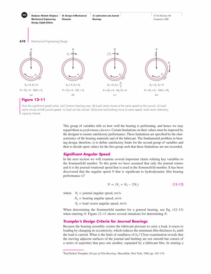
Budynas−Nisbett: Shigley’s
Mechanical Engineering
Design, Eighth Edition
III. Design of Mechanical
Elements
12. Lubrication and Journal
Bearings
610 © The McGraw−Hill
Companies, 2008
610 Mechanical Engineering Design
Figure 12–11
How the significant speed varies. (a) Common bearing case. (b) Load vector moves at the same speed as the journal. (c) Loadvector moves at half journal speed, no load can be carried. (d) Journal and bushing move at same speed, load vector stationary,capacity halved.
W
Nb = 0, Nf = 0
(a)
N = �Nj + 0 – 2(0)� = Nj N = �Nj + 0 – 2Nj� = Nj N = �Nj + 0 – 2Nj�2� = 0 N = �Nj + Nj – 2(0)� = 2Nj
Nj
W
Nb = 0, Nf = Nj
(b)
Nj
Nf
W
Nb = Nj, Nf = 0
(d )
Nj
Nb
W
Nb = 0, Nf =
(c)
Nj
Nj1
2
Nj
2
This group of variables tells us how well the bearing is performing, and hence we may
regard them as performance factors. Certain limitations on their values must be imposed by
the designer to ensure satisfactory performance. These limitations are specified by the char-
acteristics of the bearing materials and of the lubricant. The fundamental problem in bear-
ing design, therefore, is to define satisfactory limits for the second group of variables and
then to decide upon values for the first group such that these limitations are not exceeded.
Significant Angular Speed
In the next section we will examine several important charts relating key variables to
the Sommerfeld number. To this point we have assumed that only the journal rotates
and it is the journal rotational speed that is used in the Sommerfeld number. It has been
discovered that the angular speed N that is significant to hydrodynamic film bearing
performance is6
N = |Nj + Nb − 2N f | (12–13)
where Nj = journal angular speed, rev/s
Nb = bearing angular speed, rev/s
Nf = load vector angular speed, rev/s
When determining the Sommerfeld number for a general bearing, use Eq. (12–13)
when entering N. Figure 12–11 shows several situations for determining N.
Trumpler’s Design Criteria for Journal Bearings
Because the bearing assembly creates the lubricant pressure to carry a load, it reacts to
loading by changing its eccentricity, which reduces the minimum film thickness h0 until
the load is carried. What is the limit of smallness of h0? Close examination reveals that
the moving adjacent surfaces of the journal and bushing are not smooth but consist of
a series of asperities that pass one another, separated by a lubricant film. In starting a
6Paul Robert Trumpler, Design of Film Bearings, Macmillan, New York, 1966, pp. 103–119.

Budynas−Nisbett: Shigley’s
Mechanical Engineering
Design, Eighth Edition
III. Design of Mechanical
Elements
12. Lubrication and Journal
Bearings
611© The McGraw−Hill
Companies, 2008
Lubrication and Journal Bearings 611
bearing under load from rest there is metal-to-metal contact and surface asperities are
broken off, free to move and circulate with the oil. Unless a filter is provided, this debris
accumulates. Such particles have to be free to tumble at the section containing the min-
imum film thickness without snagging in a togglelike configuration, creating additional
damage and debris. Trumpler, an accomplished bearing designer, provides a throat of at
least 200 µin to pass particles from ground surfaces.7 He also provides for the influence
of size (tolerances tend to increase with size) by stipulating
h0 ≥ 0.0002 + 0.000 04d in (a)
where d is the journal diameter in inches.
A lubricant is a mixture of hydrocarbons that reacts to increasing temperature by
vaporizing the lighter components, leaving behind the heavier. This process (bearings
have lots of time) slowly increases the viscosity of the remaining lubricant, which
increases heat generation rate and elevates lubricant temperatures. This sets the stage
for future failure. For light oils, Trumpler limits the maximum film temperature Tmax to
Tmax ≤ 250◦F (b)
Some oils can operate at slightly higher temperatures. Always check with the lubricant
manufacturer.
A journal bearing often consists of a ground steel journal working against a softer,
usually nonferrous, bushing. In starting under load there is metal-to-metal contact,
abrasion, and the generation of wear particles, which, over time, can change the geo-
metry of the bushing. The starting load divided by the projected area is limited to
Wst
l D≤ 300 psi (c)
If the load on a journal bearing is suddenly increased, the increase in film temper-
ature in the annulus is immediate. Since ground vibration due to passing trucks, trains,
and earth tremors is often present, Trumpler used a design factor of 2 or more on the
running load, but not on the starting load of Eq. (c):
nd ≥ 2 (d )
Many of Trumpler’s designs are operating today, long after his consulting career is
over; clearly they constitute good advice to the beginning designer.
12–8 The Relations of the VariablesBefore proceeding to the problem of design, it is necessary to establish the relationships
between the variables. Albert A. Raimondi and John Boyd, of Westinghouse Research
Laboratories, used an iteration technique to solve Reynolds’ equation on the digital
computer.8 This is the first time such extensive data have been available for use by
designers, and consequently we shall employ them in this book.9
7Op. cit., pp. 192–194.
8A. A. Raimondi and John Boyd, “A Solution for the Finite Journal Bearing and Its Application to Analysis
and Design, Parts I, II, and III,” Trans. ASLE, vol. 1, no. 1, in Lubrication Science and Technology,
Pergamon, New York, 1958, pp. 159–209.
9See also the earlier companion paper, John Boyd and Albert A. Raimondi, “Applying Bearing Theory to the
Analysis and Design of Journal Bearings, Part I and II,” J. Appl. Mechanics, vol. 73, 1951, pp. 298–316.
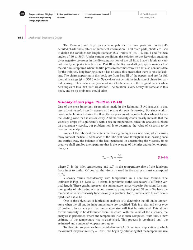
Budynas−Nisbett: Shigley’s
Mechanical Engineering
Design, Eighth Edition
III. Design of Mechanical
Elements
12. Lubrication and Journal
Bearings
612 © The McGraw−Hill
Companies, 2008
612 Mechanical Engineering Design
The Raimondi and Boyd papers were published in three parts and contain 45
detailed charts and 6 tables of numerical information. In all three parts, charts are used
to define the variables for length-diameter (l/d) ratios of 1:4, 1:2, and 1 and for beta
angles of 60 to 360◦. Under certain conditions the solution to the Reynolds equation
gives negative pressures in the diverging portion of the oil film. Since a lubricant can-
not usually support a tensile stress, Part III of the Raimondi-Boyd papers assumes that
the oil film is ruptured when the film pressure becomes zero. Part III also contains data
for the infinitely long bearing; since it has no ends, this means that there is no side leak-
age. The charts appearing in this book are from Part III of the papers, and are for full
journal bearings (β = 360◦) only. Space does not permit the inclusion of charts for par-
tial bearings. This means that you must refer to the charts in the original papers when
beta angles of less than 360◦ are desired. The notation is very nearly the same as in this
book, and so no problems should arise.
Viscosity Charts (Figs. 12–12 to 12–14)
One of the most important assumptions made in the Raimondi-Boyd analysis is that
viscosity of the lubricant is constant as it passes through the bearing. But since work is
done on the lubricant during this flow, the temperature of the oil is higher when it leaves
the loading zone than it was on entry. And the viscosity charts clearly indicate that the
viscosity drops off significantly with a rise in temperature. Since the analysis is based
on a constant viscosity, our problem now is to determine the value of viscosity to be
used in the analysis.
Some of the lubricant that enters the bearing emerges as a side flow, which carries
away some of the heat. The balance of the lubricant flows through the load-bearing zone
and carries away the balance of the heat generated. In determining the viscosity to be
used we shall employ a temperature that is the average of the inlet and outlet tempera-
tures, or
Tav = T1 + �T
2(12–14)
where T1 is the inlet temperature and �T is the temperature rise of the lubricant
from inlet to outlet. Of course, the viscosity used in the analysis must correspond
to Tav .
Viscosity varies considerably with temperature in a nonlinear fashion. The
ordinates in Figs. 12–12 to 12–14 are not logarithmic, as the decades are of differing ver-
tical length. These graphs represent the temperature versus viscosity functions for com-
mon grades of lubricating oils in both customary engineering and SI units. We have the
temperature versus viscosity function only in graphical form, unless curve fits are devel-
oped. See Table 12–1.
One of the objectives of lubrication analysis is to determine the oil outlet temper-
ature when the oil and its inlet temperature are specified. This is a trial-and-error type
of problem. In an analysis, the temperature rise will first be estimated. This allows
for the viscosity to be determined from the chart. With the value of the viscosity, the
analysis is performed where the temperature rise is then computed. With this, a new
estimate of the temperature rise is established. This process is continued until the
estimated and computed temperatures agree.
To illustrate, suppose we have decided to use SAE 30 oil in an application in which
the oil inlet temperature is T1 = 180◦F. We begin by estimating that the temperature rise
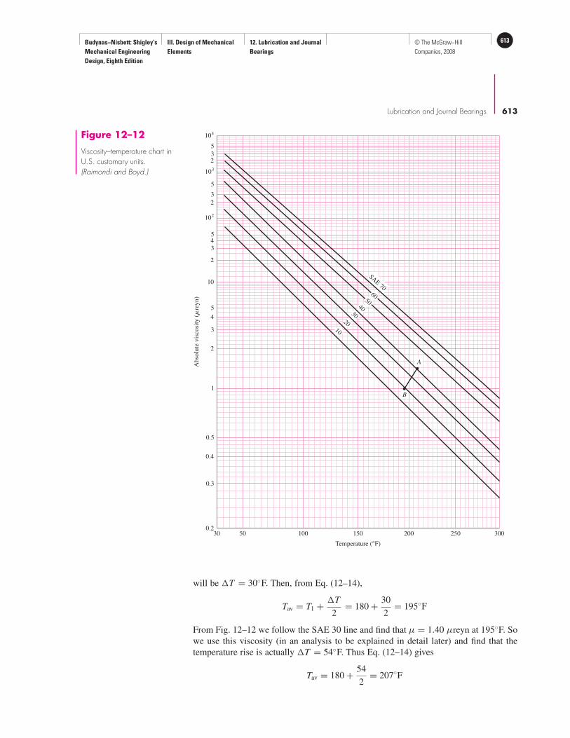
Budynas−Nisbett: Shigley’s
Mechanical Engineering
Design, Eighth Edition
III. Design of Mechanical
Elements
12. Lubrication and Journal
Bearings
613© The McGraw−Hill
Companies, 2008
Lubrication and Journal Bearings 613
Figure 12–12
Viscosity–temperature chart inU.S. customary units.(Raimondi and Boyd.)
30 50 100 150 200 250 3000.2
0.3
0.4
0.5
1
2
3
4
5
10
2
3
45
23
5
2
3
5
102
103
104
A
B
SAE 70
Temperature (°F)
Abso
lute
vis
cosi
ty (
�re
yn)
4030
2010
50
60
will be �T = 30◦F. Then, from Eq. (12–14),
Tav = T1 + �T
2= 180 + 30
2= 195◦F
From Fig. 12–12 we follow the SAE 30 line and find that µ = 1.40 µreyn at 195◦F. So
we use this viscosity (in an analysis to be explained in detail later) and find that the
temperature rise is actually �T = 54◦F. Thus Eq. (12–14) gives
Tav = 180 + 54
2= 207◦F
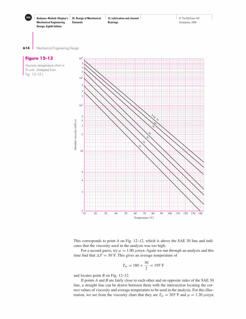
Budynas−Nisbett: Shigley’s
Mechanical Engineering
Design, Eighth Edition
III. Design of Mechanical
Elements
12. Lubrication and Journal
Bearings
614 © The McGraw−Hill
Companies, 2008
614 Mechanical Engineering Design
30
10
10 20 30 40 50 60 70 80 90 100 110 120 130 1402
3
4
5
10
2
3
4
5
102
2
3
5
103
2
3
5
104
Temperature (°C)
Abso
lute
vis
cosi
ty (
mP
a·s
)
50
60
40
20
SAE 70
Figure 12–13
Viscosity–temperature chart inSI units. (Adapted fromFig. 12–12.)
This corresponds to point A on Fig. 12–12, which is above the SAE 30 line and indi-
cates that the viscosity used in the analysis was too high.
For a second guess, try µ = 1.00 µreyn. Again we run through an analysis and this
time find that �T = 30◦F. This gives an average temperature of
Tav = 180 + 30
2= 195◦F
and locates point B on Fig. 12–12.
If points A and B are fairly close to each other and on opposite sides of the SAE 30
line, a straight line can be drawn between them with the intersection locating the cor-
rect values of viscosity and average temperature to be used in the analysis. For this illus-
tration, we see from the viscosity chart that they are Tav = 203◦F and µ = 1.20 µreyn.

Budynas−Nisbett: Shigley’s
Mechanical Engineering
Design, Eighth Edition
III. Design of Mechanical
Elements
12. Lubrication and Journal
Bearings
615© The McGraw−Hill
Companies, 2008
Lubrication and Journal Bearings 615
Figure 12–14
Chart for multiviscositylubricants. This chart wasderived from known viscositiesat two points, 100 and210°F, and the results arebelieved to be correct forother temperatures.
50 100 150 200 250 3000.2
0.3
0.4
0.5
1
2
3
4
5
10
2
3
45
102
23
45
103
Temperature (°F)
Ab
solu
te v
isco
sity
(�
rey
n)
20W – 50
20W – 40
10W – 30
5W – 30
20W10W
Viscosity ConstantOil Grade, SAE �0, reyn b, °F
10 0.0158(10−6) 1157.5
20 0.0136(10−6) 1271.6
30 0.0141(10−6) 1360.0
40 0.0121(10−6) 1474.4
50 0.0170(10−6) 1509.6
60 0.0187(10−6) 1564.0
∗� � �0 exp [b/(T � 95)], T in °F.
Table 12–1
Curve Fits* to Approxi-
mate the Viscosity versus
Temperature Functions for
SAE Grades 10 to 60
Source: A. S. Seireg and S.Dandage, “Empirical DesignProcedure for the Thermody-namic Behavior of JournalBearings,” J. LubricationTechnology, vol. 104, April1982, pp. 135–148.

Budynas−Nisbett: Shigley’s
Mechanical Engineering
Design, Eighth Edition
III. Design of Mechanical
Elements
12. Lubrication and Journal
Bearings
616 © The McGraw−Hill
Companies, 2008
616 Mechanical Engineering Design
Figure 12–16
Chart for minimum film-thickness variable and eccentricity ratio. The left boundary of the zone defines the optimal h0 for minimum friction;the right boundary is optimum h0 for load. (Raimondi and Boyd.)
0 0.01 0.02 0.04 0.06 0.08 0.1 0.2 0.4 0.6 0.8 1.0 2 4 6 8 100
0.1
0.2
0.3
0.4
0.5
0.6
0.7
0.8
0.9
1.0
1.0
0.9
0.8
0.7
0.6
0.5
0.4
0.3
0.2
0.1
0
Bearing characteristic number, S = ( )2rc
�N
P
Min
imum
-fil
m-t
hic
knes
s var
iab
le (d
imen
sio
nle
ss)
h0 c
Ecc
entr
icit
y r
atio
(
dim
ensi
on
less
)
l ⁄d= ∞
1
1⁄ 2
Max. W
Min
.f
1⁄ 4
Figure 12–15
Polar diagram of thefilm–pressure distributionshowing the notation used.(Raimondi and Boyd.)
W
pmax
pmax
p0
�
Film pressure p
h0
O
eO'
N
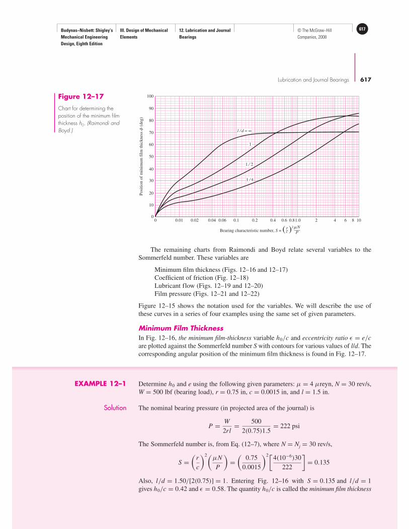
Budynas−Nisbett: Shigley’s
Mechanical Engineering
Design, Eighth Edition
III. Design of Mechanical
Elements
12. Lubrication and Journal
Bearings
617© The McGraw−Hill
Companies, 2008
Lubrication and Journal Bearings 617
Figure 12–17
Chart for determining theposition of the minimum filmthickness h0. (Raimondi andBoyd.)
0 0.01 0.02 0.04 0.06 0.1 0.2 0.4 0.6 0.81.0 2 4 6 8 100
10
20
30
40
50
60
70
80
90
100
Bearing characteristic number, S = ( )2rc
�N
P
Po
siti
on
of
min
imu
m f
ilm
th
ick
nes
s �
(d
eg)
l ⁄ d = ∞
1
1 ⁄ 2
1 ⁄ 4
The remaining charts from Raimondi and Boyd relate several variables to the
Sommerfeld number. These variables are
Minimum film thickness (Figs. 12–16 and 12–17)
Coefficient of friction (Fig. 12–18)
Lubricant flow (Figs. 12–19 and 12–20)
Film pressure (Figs. 12–21 and 12–22)
Figure 12–15 shows the notation used for the variables. We will describe the use of
these curves in a series of four examples using the same set of given parameters.
Minimum Film Thickness
In Fig. 12–16, the minimum film-thickness variable h0/c and eccentricity ratio ε = e/c
are plotted against the Sommerfeld number S with contours for various values of l/d. The
corresponding angular position of the minimum film thickness is found in Fig. 12–17.
EXAMPLE 12–1 Determine h0 and e using the following given parameters: µ = 4 µreyn, N = 30 rev/s,
W = 500 lbf (bearing load), r = 0.75 in, c = 0.0015 in, and l = 1.5 in.
Solution The nominal bearing pressure (in projected area of the journal) is
P = W
2rl= 500
2(0.75)1.5= 222 psi
The Sommerfeld number is, from Eq. (12–7), where N = Nj = 30 rev/s,
S =(
r
c
)2(µN
P
)
=(
0.75
0.0015
)2[4(10−6)30
222
]
= 0.135
Also, l/d = 1.50/[2(0.75)] = 1. Entering Fig. 12–16 with S = 0.135 and l/d = 1
gives h0/c = 0.42 and ε = 0.58. The quantity h0/c is called the minimum film thickness

Budynas−Nisbett: Shigley’s
Mechanical Engineering
Design, Eighth Edition
III. Design of Mechanical
Elements
12. Lubrication and Journal
Bearings
618 © The McGraw−Hill
Companies, 2008
618 Mechanical Engineering Design
variable. Since c = 0.0015 in, the minimum film thickness h0 is
h0 = 0.42(0.0015) = 0.000 63 in
We can find the angular location φ of the minimum film thickness from the chart of
Fig. 12–17. Entering with S = 0.135 and l/d = 1 gives φ = 53◦.
The eccentricity ratio is ε = e/c = 0.58. This means the eccentricity e is
e = 0.58(0.0015) = 0.000 87 in
Note that if the journal is centered in the bushing, e = 0 and h0 = c, correspond-
ing to a very light (zero) load. Since e = 0, ε = 0. As the load is increased the journal
displaces downward; the limiting position is reached when h0 = 0 and e = c, that is,
when the journal touches the bushing. For this condition the eccentricity ratio is unity.
Since h0 = c − e, dividing both sides by c, we have
h0
c= 1 − ε
Design optima are sometimes maximum load, which is a load-carrying character-
istic of the bearing, and sometimes minimum parasitic power loss or minimum coeffi-
cient of friction. Dashed lines appear on Fig. 12–16 for maximum load and minimum
coefficient of friction, so you can easily favor one of maximum load or minimum coef-
ficient of friction, but not both. The zone between the two dashed-line contours might
be considered a desirable location for a design point.
Coefficient of Friction
The friction chart, Fig. 12–18, has the friction variable (r/c) f plotted against
Sommerfeld number S with contours for various values of the l/d ratio.
EXAMPLE 12–2 Using the parameters given in Ex. 12–1, determine the coefficient of friction, the torque
to overcome friction, and the power loss to friction.
Solution We enter Fig. 12–18 with S = 0.135 and l/d = 1 and find (r/c) f = 3.50. The coeffi-
cient of friction f is
f = 3.50 c/r = 3.50(0.0015/0.75) = 0.0070
The friction torque on the journal is
T = f Wr = 0.007(500)0.75 = 2.62 lbf · in
The power loss in horsepower is
(hp)loss = T N
1050= 2.62(30)
1050= 0.075 hp
or, expressed in Btu/s,
H = 2πT N
778(12)= 2π(2.62)30
778(12)= 0.0529 Btu/s

Budynas−Nisbett: Shigley’s
Mechanical Engineering
Design, Eighth Edition
III. Design of Mechanical
Elements
12. Lubrication and Journal
Bearings
619© The McGraw−Hill
Companies, 2008
Lubrication and Journal Bearings 619
Lubricant Flow
Figures 12–19 and 12–20 are used to determine the lubricant flow and side flow.
EXAMPLE 12–3 Continuing with the parameters of Ex. 12–1, determine the total volumetric flow rate Q
and the side flow rate Qs .
Solution To estimate the lubricant flow, enter Fig. 12–19 with S = 0.135 and l/d = 1 to obtain
Q/(rcNl) = 4.28. The total volumetric flow rate is
Q = 4.28rcNl = 4.28(0.75)0.0015(30)1.5 = 0.217 in3/s
From Fig. 12–20 we find the flow ratio Qs/Q = 0.655 and Qs is
Qs = 0.655Q = 0.655(0.217) = 0.142 in3/s
Figure 12–18
Chart for coefficient-of-friction variable; note that Petroff’s equation is the asymptote. (Raimondi and Boyd.)
∞
1
1 ⁄ 2
l ⁄d = 1 ⁄ 4
0 0.01 0.02 0.04 0.06 0.1 0.2 0.4 0.6 0.8 1.0 2 4 6 8 100
1
2
3
4
5
10
2
3
4
5
102
2
Bearing characteristic number, S = ( )2rc
�N
P
Coef
fici
ent-
of-
fric
tion v
aria
ble
f
(dim
ensi
onle
ss)
r c

Budynas−Nisbett: Shigley’s
Mechanical Engineering
Design, Eighth Edition
III. Design of Mechanical
Elements
12. Lubrication and Journal
Bearings
620 © The McGraw−Hill
Companies, 2008
620 Mechanical Engineering Design
0 0.01 0.02 0.04 0.06 0.1 0.2 0.4 0.6 0.8 1.0 2 4 6 8 100
1
2
3
4
5
6
Bearing characteristic number, S = ( )2rc
�N
P
Flo
w v
aria
ble
(
dim
ensi
onle
ss)
Q
rcN
l
l ⁄ d = 1 ⁄ 4
l ⁄ d = 1 ⁄ 2
l ⁄ d = 1
l⁄ d
=∞
Figure 12–19
Chart for flow variable. Note:Not for pressure-fed bearings.(Raimondi and Boyd.)
Figure 12–20
Chart for determining the ratioof side flow to total flow.(Raimondi and Boyd.)
0 0.01 0.02 0.04 0.06 0.1 0.2 0.4 0.6 1.0 2 4 6 8 100
0.1
0.2
0.3
0.4
0.5
0.6
0.7
0.8
0.9
1.0
Bearing characteristic number, S = ( )2rc
�N
P
Flo
w r
atio
Qs
Q
l ⁄ d = 1 ⁄ 4
1⁄ 2
1
l ⁄d = ∞

Budynas−Nisbett: Shigley’s
Mechanical Engineering
Design, Eighth Edition
III. Design of Mechanical
Elements
12. Lubrication and Journal
Bearings
621© The McGraw−Hill
Companies, 2008
Lubrication and Journal Bearings 621
Figure 12–21
Chart for determining themaximum film pressure. Note:Not for pressure-fed bearings.(Raimondi and Boyd.)
l ⁄d = ∞
1
1 ⁄ 2
1 ⁄ 4
0 0.01 0.02 0.04 0.06 0.1 0.2 0.4 0.6 0.8 1.0 2 4 6 8 100
0.1
0.2
0.3
0.4
0.5
0.6
0.7
0.8
0.9
1.0
Bearing characteristic number, S = ( )2rc
�N
P
Max
imum
-fil
m-p
ress
ure
rat
io(
)
Pp
max
psi
psi
g
The side leakage Qs is from the lower part of the bearing, where the internal pressure
is above atmospheric pressure. The leakage forms a fillet at the journal-bushing exter-
nal junction, and it is carried by journal motion to the top of the bushing, where the
internal pressure is below atmospheric pressure and the gap is much larger, to be
“sucked in” and returned to the lubricant sump. That portion of side leakage that leaks
away from the bearing has to be made up by adding oil to the bearing sump periodically
by maintenance personnel.
Film Pressure
The maximum pressure developed in the film can be estimated by finding the pressure
ratio P/pmax from the chart in Fig. 12–21. The locations where the terminating and
maximum pressures occur, as defined in Fig 12–15, are determined from Fig. 12–22.
EXAMPLE 12–4 Using the parameters given in Ex. 12–1, determine the maximum film pressure and the
locations of the maximum and terminating pressures.
Solution Entering Fig. 12–21 with S = 0.135 and l/d = 1, we find P/pmax = 0.42. The maxi-
mum pressure pmax is therefore
pmax = P
0.42= 222
0.42= 529 psi
With S = 0.135 and l/d = 1, from Fig. 12–22, θpmax= 18.5◦ and the terminating posi-
tion θp0is 75◦.

Budynas−Nisbett: Shigley’s
Mechanical Engineering
Design, Eighth Edition
III. Design of Mechanical
Elements
12. Lubrication and Journal
Bearings
622 © The McGraw−Hill
Companies, 2008
622 Mechanical Engineering Design
Examples 12–1 to 12–4 demonstrate how the Raimondi and Boyd charts are used.
It should be clear that we do not have journal-bearing parametric relations as equations,
but in the form of charts. Moreover, the examples were simple because the steady-state
equivalent viscosity was given. We will now show how the average film temperature
(and the corresponding viscosity) is found from energy considerations.
Lubricant Temperature Rise
The temperature of the lubricant rises until the rate at which work is done by the jour-
nal on the film through fluid shear is the same as the rate at which heat is transferred to
the greater surroundings. The specific arrangement of the bearing plumbing affects the
quantitative relationships. See Fig. 12–23. A lubricant sump (internal or external to the
bearing housing) supplies lubricant at sump temperature Ts to the bearing annulus at
temperature Ts = T1. The lubricant passes once around the bushing and is delivered at
a higher lubricant temperature T1 + �T to the sump. Some of the lubricant leaks out of
the bearing at a mixing-cup temperature of T1 + �T/2 and is returned to the sump. The
sump may be a keyway-like groove in the bearing cap or a larger chamber up to half the
bearing circumference. It can occupy “all” of the bearing cap of a split bearing. In such
a bearing the side leakage occurs from the lower portion and is sucked back in, into the
ruptured film arc. The sump could be well removed from the journal-bushing interface.
0 0.01 0.02 0.04 0.06 0.08 0.1 0.2 0.4 0.6 0.8 1.0 2 4 6 8 100
10
20
30
40
50
60
70
80
90
100
0
5
10
15
20
25
l ⁄d = ∞ 11 ⁄ 2
1 ⁄ 4
1 ⁄ 2
1 ⁄ 4
1
∞
Bearing characteristic number, S = ( )2rc
�N
Pp0
pmax
Ter
min
atin
g p
osi
tion o
f fi
lm
p0 (
deg
)
Posi
tion o
f m
axim
um
fil
m p
ress
ure
p m
ax(d
eg)
Figure 12–22
Chart for finding the terminating position of the lubricant film and the position of maximum film pressure. (Raimondi and Boyd.)

Budynas−Nisbett: Shigley’s
Mechanical Engineering
Design, Eighth Edition
III. Design of Mechanical
Elements
12. Lubrication and Journal
Bearings
623© The McGraw−Hill
Companies, 2008
Lubrication and Journal Bearings 623
Let
Q = volumetric oil-flow rate into the bearing, in3/s
Qs = volumetric side-flow leakage rate out of the bearing and to the sump, in3/s
Q − Qs = volumetric oil-flow discharge from annulus to sump, in3/s
T1 = oil inlet temperature (equal to sump temperature Ts ), ◦F
�T = temperature rise in oil between inlet and outlet, ◦F
ρ = lubricant density, lbm/in3
Cp = specific heat capacity of lubricant, Btu/(lbm · ◦F)
J = Joulean heat equivalent, in · lbf/Btu
H = heat rate, Btu/s
Using the sump as a control region, we can write an enthalpy balance. Using T1 as the
datum temperature gives
Hloss = ρCp Qs�T/2 + ρCp(Q − Qs)�T = ρCp Q�T
(
1 − 1
2
Qs
Q
)
(a)
The thermal energy loss at steady state Hloss is equal to the rate the journal does work
on the film is Hloss = W = 2πT N/J . The torque T = f Wr , the load in terms of pres-
sure is W = 2Prl , and multiplying numerator and denominator by the clearance c gives
Hloss = 4π Prl Nc
J
r f
c(b)
Equating Eqs. (a) and (b) and rearranging results in
JρCp �T
4π P= r f/c
(1 − 0.5Qs/Q) [Q/(rcNl)](c)
For common petroleum lubricants ρ = 0.0311 lbm/in3, Cp = 0.42 Btu/(lbm · ◦F), and
J = 778(12) = 9336 in · lbf/Btu; therefore the left term of Eq. (c) is
JρCp �T
4π P= 9336(0.0311)0.42�TF
4π Ppsi
= 9.70�TF
Ppsi
thus
9.70�TF
Ppsi
= r f/c(
1 − 12
Qs/Q)
[Q/(rcNj l)](12–15)
Figure 12–23
Schematic of a journalbearing with an external sumpwith cooling; lubricant makesone pass before returning tothe sump.
Supply
Q, T1Return
Q – Qs
T1 + ∆T
End leakage
Qs, T1 + ∆T2
T1 +T1∆T2
T1 + ∆T
Q Qs
Q – QsSump
T1
Heat loss rate
Hloss
Control
surface
(a) (b)
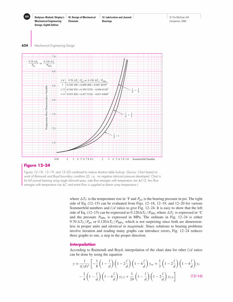
Budynas−Nisbett: Shigley’s
Mechanical Engineering
Design, Eighth Edition
III. Design of Mechanical
Elements
12. Lubrication and Journal
Bearings
624 © The McGraw−Hill
Companies, 2008
624 Mechanical Engineering Design
Figure 12–24
Figures 12–18, 12–19, and 12–20 combined to reduce iterative table look-up. (Source: Chart based onwork of Raimondi and Boyd boundary condition (2), i.e., no negative lubricant pressure developed. Chart isfor full journal bearing using single lubricant pass, side flow emerges with temperature rise �T/2, thru flowemerges with temperature rise �T, and entire flow is supplied at datum sump temperature.)
0.01 2 3 4 5 6 7 8 0.1 2 3 4 5 6 7 8 1.0 Sommerfeld Number
l ⁄d
1 0.349 109 + 6.009 40S + 0.047 467S2
0.394 552 + 6.392 527S − 0.036 013S2
0.933 828 + 6.437 512S − 0.011 048S2
1 ⁄ 2
1 ⁄ 4
9.70 ∆TF ⁄ Ppsi∆TC ⁄ PMPaor 0.120
9.70 ∆TF
Ppsi
0.120 ∆TC
PMPa
or
6.0
7.0
5.0
4.0
3.0
2.0
1.0
ld
= 1
ld
12
=
ld
14
=
Tem
per
ature
Ris
e D
imen
sionle
ss V
aria
ble
where �TF is the temperature rise in ◦F and Ppsi is the bearing pressure in psi. The right
side of Eq. (12–15) can be evaluated from Figs. 12–18, 12–19, and 12–20 for various
Sommerfeld numbers and l/d ratios to give Fig. 12–24. It is easy to show that the left
side of Eq. (12–15) can be expressed as 0.120�TC/PMPa where �TC is expressed in ◦C
and the pressure PMPa is expressed in MPa. The ordinate in Fig. 12–24 is either
9.70 �TF/Ppsi or 0.120�TC/PMPa , which is not surprising since both are dimension-
less in proper units and identical in magnitude. Since solutions to bearing problems
involve iteration and reading many graphs can introduce errors, Fig. 12–24 reduces
three graphs to one, a step in the proper direction.
Interpolation
According to Raimondi and Boyd, interpolation of the chart data for other l/d ratios
can be done by using the equation
y = 1
(l/d)3
[
−1
8
(
1 − l
d
)(
1 − 2l
d
)(
1 − 4l
d
)
y∞ + 1
3
(
1 − 2l
d
)(
1 − 4l
d
)
y1
− 1
4
(
1 − l
d
)(
1 − 4l
d
)
y1/2 + 1
24
(
1 − l
d
)(
1 − 2l
d
)
y1/4
]
(12–16)

Budynas−Nisbett: Shigley’s
Mechanical Engineering
Design, Eighth Edition
III. Design of Mechanical
Elements
12. Lubrication and Journal
Bearings
625© The McGraw−Hill
Companies, 2008
Lubrication and Journal Bearings 625
where y is the desired variable within the interval ∞ > l/d > 14
and y∞, y1, y1/2, and
y1/4 are the variables corresponding to l/d ratios of ∞, 1, 12, and 1
4, respectively.
12–9 Steady-State Conditions in Self-Contained BearingsThe case in which the lubricant carries away all of the enthalpy increase from the
journal-bushing pair has already been discussed. Bearings in which the warm lubricant
stays within the bearing housing will now be addressed. These bearings are called self-
contained bearings because the lubricant sump is within the bearing housing and the
lubricant is cooled within the housing. These bearings are described as pillow-block or
pedestal bearings. They find use on fans, blowers, pumps, and motors, for example.
Integral to design considerations for these bearings is dissipating heat from the bearing
housing to the surroundings at the same rate that enthalpy is being generated within the
fluid film.
In a self-contained bearing the sump can be positioned as a keywaylike cavity in the
bushing, the ends of the cavity not penetrating the end planes of the bushing. Film oil
exits the annulus at about one-half of the relative peripheral speeds of the journal and
bushing and slowly tumbles the sump lubricant, mixing with the sump contents. Since
the film in the top “half” of the cap has cavitated, it contributes essentially nothing to the
support of the load, but it does contribute friction. Bearing caps are in use in which
the “keyway” sump is expanded peripherally to encompass the top half of the bearing.
This reduces friction for the same load, but the included angle β of the bearing has been
reduced to 180◦. Charts for this case were included in the Raimondi and Boyd paper.
The heat given up by the bearing housing may be estimated from the equation
Hloss = hCR A(Tb − T∞) (12–17)
where Hloss = heat dissipated, Btu/h
hCR = combined overall coefficient of radiation and convection heat
transfer, Btu/(h · ft2 · ◦F)
A = surface area of bearing housing, ft2
Tb = surface temperature of the housing, ◦F
T∞ = ambient temperature, ◦F
The overall coefficient hCR depends on the material, surface coating, geometry, even the
roughness, the temperature difference between the housing and surrounding objects,
and air velocity. After Karelitz,10 and others, in ordinary industrial environments, the
overall coefficient hCR can be treated as a constant. Some representative values are
hCR =
2 Btu/(h · ft2 · ◦F) for still air
2.7 Btu/(h · ft2 · ◦F) for shaft-stirred air
5.9 Btu/(h · ft2 · ◦F) for air moving at 500 ft/min
(12–18)
An expression similar to Eq. (12–17) can be written for the temperature difference
Tf − Tb between the lubricant film and the housing surface. This is possible because
the bushing and housing are metal and very nearly isothermal. If one defines Tf as the
average film temperature (halfway between the lubricant inlet temperature Ts and the
10G. B. Karelitz, “Heat Dissipation in Self-Contained Bearings,” Trans. ASME, Vol. 64, 1942, p. 463; D. C.
Lemmon and E. R. Booser, “Bearing Oil-Ring Performance,” Trans. ASME, J. Bas. Engin., Vol. 88, 1960,
p. 327.

Budynas−Nisbett: Shigley’s
Mechanical Engineering
Design, Eighth Edition
III. Design of Mechanical
Elements
12. Lubrication and Journal
Bearings
626 © The McGraw−Hill
Companies, 2008
626 Mechanical Engineering Design
outlet temperature Ts + �T ), then the following proportionality has been observed
between Tf − Tb and the difference between the housing surface temperature and the
ambient temperature, Tb − T∞:
Tf − Tb = α(Tb − T∞) (a)
where Tf is the average film temperature and α is a constant depending on the lubrica-
tion scheme and the bearing housing geometry. Equation (a) may be used to estimate
the bearing housing temperature. Table 12–2 provides some guidance concerning suit-
able values of α. The work of Karelitz allows the broadening of the application of the
charts of Raimondi and Boyd, to be applied to a variety of bearings beyond the natural
circulation pillow-block bearing.
Solving Eq. (a) for Tb and substituting into Eq. (12–17) gives the bearing heat loss
rate to the surroundings as
Hloss = hCR A
1 + α(Tf − T∞) (12–19a)
and rewriting Eq. (a) gives
Tb = Tf + αT∞1 + α
(12–19b)
In beginning a steady-state analysis the average film temperature is unknown, hence the
viscosity of the lubricant in a self-contained bearing is unknown. Finding the equilibrium
temperatures is an iterative process wherein a trial average film temperature (and the
corresponding viscosity) is used to compare the heat generation rate and the heat loss
rate. An adjustment is made to bring these two heat rates into agreement. This can be
done on paper with a tabular array to help adjust Tf to achieve equality between heat
generation and loss rates. A root-finding algorithm can be used. Even a simple one can
be programmed for a digital computer.
Because of the shearing action there is a uniformly distributed energy release in the
lubricant that heats the lubricant as it works its way around the bearing. The tempera-
ture is uniform in the radial direction but increases from the sump temperature Ts by
an amount �T during the lubricant pass. The exiting lubricant mixes with the sump
contents, being cooled to sump temperature. The lubricant in the sump is cooled
because the bushing and housing metal are at a nearly uniform lower temperature
because of heat losses by convection and radiation to the surroundings at ambient tem-
perature T∞. In the usual configurations of such bearings, the bushing and housing
metal temperature is approximately midway between the average film temperature
Tf = Ts + �T/2 and the ambient temperature T∞. The heat generation rate Hgen, at
steady state, is equal to the work rate from the frictional torque T. Expressing this in
Btu/h requires the conversion constants 2545 Btu/(hp · h) and 1050 (lbf · in)(rev/s)/hp
results in Hgen = 2545 T N/1050. Then from Eq. (b), Sec. 12–3, the torque is
Lubrication System Conditions Range of
Oil ring Moving air 1–2
Still air 12–1
Oil bath Moving air 12–1
Still air 15– 2
5
Table 12–2

Budynas−Nisbett: Shigley’s
Mechanical Engineering
Design, Eighth Edition
III. Design of Mechanical
Elements
12. Lubrication and Journal
Bearings
627© The McGraw−Hill
Companies, 2008
Lubrication and Journal Bearings 627
T = 4π2r3lµ/c, resulting in
Hgen = 2545
1050
4π2r3lµN
cN = 95.69µN 2lr3
c(b)
Equating this to Eq. (12–19a) and solving for Tf gives
Tf = T∞ + 95.69(1 + α)µN 2lr3
hCR Ac (12–20)
EXAMPLE 12–5 Consider a pillow-block bearing with a keyway sump, whose journal rotates at
900 rev/min in shaft-stirred air at 70◦F with α = 1. The lateral area of the bearing is
40 in2. The lubricant is SAE grade 20 oil. The gravity radial load is 100 lbf and the l/d
ratio is unity. The bearing has a journal diameter of 2.000 + 0.000/−0.002 in, a bush-
ing bore of 2.002 + 0.004/−0.000 in. For a minimum clearance assembly estimate the
steady-state temperatures as well as the minimum film thickness and coefficient of
friction.
Solution The minimum radial clearance, cmin, is
cmin = 2.002 − 2.000
2= 0.001 in
P = W
ld= 100
(2)2= 25 psi
S =(
r
c
)2µN
P=(
1
0.001
)2µ′(15)
106(25)= 0.6 µ′
where µ′ is viscosity in µreyn. The friction horsepower loss, (hp) f , is found as follows:
(hp) f = f Wr N
1050= W Nc
1050
f r
c= 100(900/60)0.001
1050
f r
c= 0.001 429
f r
chp
The heat generation rate Hgen, in Btu/h, is
Hgen = 2545(hp) f = 2545(0.001 429) f r/c = 3.637 f r/c Btu/h
From Eq. (12–19a) with hCR = 2.7 Btu/(h · ft2 · °F), the rate of heat loss to the envi-
ronment Hloss is
Hloss = hCR A
α + 1(Tf − 70) = 2.7(40/144)
(1 + 1)(Tf − 70) = 0.375(Tf − 70) Btu/h
Build a table as follows for trial values of Tf of 190 and 195°F:
Trial Tf � S fr/c Hgen Hloss
190 1.15 0.69 13.6 49.5 45.0
195 1.03 0.62 12.2 44.4 46.9

Budynas−Nisbett: Shigley’s
Mechanical Engineering
Design, Eighth Edition
III. Design of Mechanical
Elements
12. Lubrication and Journal
Bearings
628 © The McGraw−Hill
Companies, 2008
628 Mechanical Engineering Design
The temperature at which Hgen = Hloss = 46.3 Btu/h is 193.4◦F. Rounding Tf to
193◦F we find µ′ = 1.08 µreyn and S = 0.6(1.08) = 0.65. From Fig. 12–24,
9.70� TF/P = 4.25°F/psi and thus
�TF = 4.25P/9.70 = 4.25(25)/9.70 = 11.0◦F
T1 = Ts = Tf − �T/2 = 193 − 11/2 = 187.5◦ F
Tmax = T1 + �TF = 187.5 + 11 = 198.5◦F
From Eq. (12–19b)
Tb = Tf + αT∞1 + α
= 193 + (1)70
1 + 1= 131.5◦F
with S = 0.65, the minimum film thickness from Fig. 12–16 is
h0 = h0
cc = 0.79(0.001) = 0.000 79 in
The coefficient of friction from Fig. 12–18 is
f = f r
c
c
r= 12.8
0.001
1= 0.012 8
The parasitic friction torque T is
T = f Wr = 0.012 8(100)(1) = 1.28 lbf · in
12–10 ClearanceIn designing a journal bearing for thick-film lubrication, the engineer must select the
grade of oil to be used, together with suitable values for P, N, r, c, and l. A poor selec-
tion of these or inadequate control of them during manufacture or in use may result in
a film that is too thin, so that the oil flow is insufficient, causing the bearing to overheat
and, eventually, fail. Furthermore, the radial clearance c is difficult to hold accurate dur-
ing manufacture, and it may increase because of wear. What is the effect of an entire
range of radial clearances, expected in manufacture, and what will happen to the bear-
ing performance if c increases because of wear? Most of these questions can be
answered and the design optimized by plotting curves of the performance as functions
of the quantities over which the designer has control.
Figure 12–25 shows the results obtained when the performance of a particular bear-
ing is calculated for a whole range of radial clearances and is plotted with clearance as
the independent variable. The bearing used for this graph is the one of Examples 12–1
to 12–4 with SAE 20 oil at an inlet temperature of 100◦F. The graph shows that if
the clearance is too tight, the temperature will be too high and the minimum film thick-
ness too low. High temperatures may cause the bearing to fail by fatigue. If the oil film
is too thin, dirt particles may be unable to pass without scoring or may embed them-
selves in the bearing. In either event, there will be excessive wear and friction, result-
ing in high temperatures and possible seizing.
To investigate the problem in more detail, Table 12–3 was prepared using the two
types of preferred running fits that seem to be most useful for journal-bearing design

Budynas−Nisbett: Shigley’s
Mechanical Engineering
Design, Eighth Edition
III. Design of Mechanical
Elements
12. Lubrication and Journal
Bearings
629© The McGraw−Hill
Companies, 2008
Lubrication and Journal Bearings 629
Table 12–3
Maximum, Minimum,
and Average Clearances
for 1.5-in-Diameter
Journal Bearings Based
on Type of Fit
Clearance c, in
Type of Fit Symbol Maximum Average Minimum
Close-running H8/f7 0.001 75 0.001 125 0.000 5
Free-running H9/d9 0.003 95 0.002 75 0.001 55
Table 12–4
Performance of
1.5-in-Diameter Journal
Bearing with Various
Clearances. (SAE 20
Lubricant, T1 = 100°F,
N = 30 r/s, W =500 lbf, L = 1.5 in)
c, in T2, °F h0, in f Q, in3/s, H, Btu/s
0.000 5 226 0.000 38 0.011 3 0.061 0.086
0.001 125 142 0.000 65 0.009 0 0.153 0.068
0.001 55 133 0.000 77 0.008 7 0.218 0.066
0.001 75 128 0.000 76 0.008 4 0.252 0.064
0.002 75 118 0.000 73 0.007 9 0.419 0.060
0.003 95 113 0.000 69 0.007 7 0.617 0.059
(see Table 7–9), p. 385. The results shown in Table 12–3 were obtained by using Eqs.
(7–36) and (7–37) of Sec. 7–8. Notice that there is a slight overlap, but the range of
clearances for the free-running fit is about twice that of the close-running fit.
The six clearances of Table 12–3 were used in a computer program to obtain the
numerical results shown in Table 12–4. These conform to the results of Fig. 12–25, too.
Both the table and the figure show that a tight clearance results in a high temperature.
Figure 12–26 can be used to estimate an upper temperature limit when the characteris-
tics of the application are known.
It would seem that a large clearance will permit the dirt particles to pass through
and also will permit a large flow of oil, as indicated in Table 12–4. This lowers the tem-
perature and increases the life of the bearing. However, if the clearance becomes too
Figure 12–25
A plot of some performancecharacteristics of the bearingof Exs. 12–1 to 12–4 forradial clearances of 0.0005to 0.003 in. The bearingoutlet temperature isdesignated T2. New bearingsshould be designed for theshaded zone, because wearwill move the operating pointto the right.
0.0005 in
Q
Q
T2
T2
H
H
h0
h0
0 0.5 1.0 1.5 2.0 2.5 3.00
Radial clearance c (10−3 in)

Budynas−Nisbett: Shigley’s
Mechanical Engineering
Design, Eighth Edition
III. Design of Mechanical
Elements
12. Lubrication and Journal
Bearings
630 © The McGraw−Hill
Companies, 2008
630 Mechanical Engineering Design
large, the bearing becomes noisy and the minimum film thickness begins to decrease
again.
In between these two limitations there exists a rather large range of clearances that
will result in satisfactory bearing performance.
When both the production tolerance and the future wear on the bearing are consid-
ered, it is seen, from Fig. 12–25, that the best compromise is a clearance range slightly
to the left of the top of the minimum-film-thickness curve. In this way, future wear will
move the operating point to the right and increase the film thickness and decrease the
operating temperature.
12–11 Pressure-Fed BearingsThe load-carrying capacity of self-contained natural-circulating journal bearings is
quite restricted. The factor limiting better performance is the heat-dissipation capability
of the bearing. A first thought of a way to increase heat dissipation is to cool the sump
with an external fluid such as water. The high-temperature problem is in the film where
the heat is generated but cooling is not possible in the film until later. This does not pro-
tect against exceeding the maximum allowable temperature of the lubricant. A second
alternative is to reduce the temperature rise in the film by dramatically increasing the
rate of lubricant flow. The lubricant itself is reducing the temperature rise. A water-
cooled sump may still be in the picture. To increase lubricant flow, an external pump
must be used with lubricant supplied at pressures of tens of pounds per square inch
gage. Because the lubricant is supplied to the bearing under pressure, such bearings are
called pressure-fed bearings.
To force a greater flow through the bearing and thus obtain an increased cooling
effect, a common practice is to use a circumferential groove at the center of the bearing,
with an oil-supply hole located opposite the load-bearing zone. Such a bearing is shown
in Fig. 12–27. The effect of the groove is to create two half-bearings, each having a
smaller l/d ratio than the original. The groove divides the pressure-distribution curve
into two lobes and reduces the minimum film thickness, but it has wide acceptance
among lubrication engineers because such bearings carry more load without overheating.
To set up a method of solution for oil flow, we shall assume a groove ample enough
that the pressure drop in the groove itself is small. Initially we will neglect eccentricity
and then apply a correction factor for this condition. The oil flow, then, is the amount
that flows out of the two halves of the bearing in the direction of the concentric shaft.
If we neglect the rotation of the shaft, the flow of the lubricant is caused by the supply
Figure 12–26
Temperature limits for mineraloils. The lower limit is for oilscontaining antioxidants andapplies when oxygen supply isunlimited. The upper limitapplies when insignificantoxygen is present. The life inthe shaded zone depends onthe amount of oxygen andcatalysts present. (Source: M. J. Neale (ed.),Tribology Handbook, SectionB1, Newnes-Butterworth,London, 1975.)
1 10 100 1000 10 0000
100
200
300
400
500
Life (h)
Tem
per
ature
(°C
)
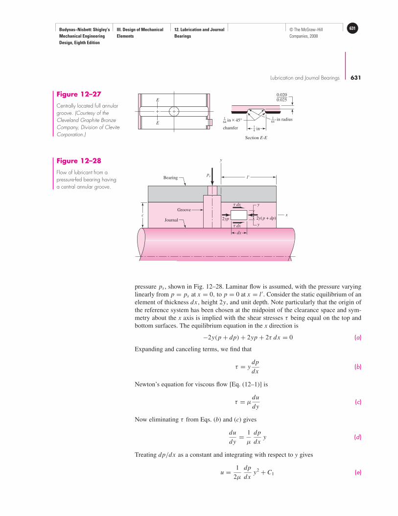
Budynas−Nisbett: Shigley’s
Mechanical Engineering
Design, Eighth Edition
III. Design of Mechanical
Elements
12. Lubrication and Journal
Bearings
631© The McGraw−Hill
Companies, 2008
Lubrication and Journal Bearings 631
pressure ps , shown in Fig. 12–28. Laminar flow is assumed, with the pressure varying
linearly from p = ps at x = 0, to p = 0 at x = l ′. Consider the static equilibrium of an
element of thickness dx , height 2y, and unit depth. Note particularly that the origin of
the reference system has been chosen at the midpoint of the clearance space and sym-
metry about the x axis is implied with the shear stresses τ being equal on the top and
bottom surfaces. The equilibrium equation in the x direction is
−2y(p + dp) + 2yp + 2τ dx = 0 (a)
Expanding and canceling terms, we find that
τ = ydp
dx(b)
Newton’s equation for viscous flow [Eq. (12–1)] is
τ = µdu
dy(c)
Now eliminating τ from Eqs. (b) and (c) gives
du
dy= 1
µ
dp
dxy (d)
Treating dp/dx as a constant and integrating with respect to y gives
u = 1
2µ
dp
dxy2 + C1 (e)
Bearing
Journal
Groove
ps
c
y
l'
x
dx
2yp
� dx
� dx y
y
2y(p + dp)
Figure 12–28
Flow of lubricant from apressure-fed bearing havinga central annular groove.
E
E
Section E-E
chamfer
0.0200.025
1
64- in radius1
64 in × 45°
1
4 in
Figure 12–27
Centrally located full annulargroove. (Courtesy of theCleveland Graphite BronzeCompany, Division of CleviteCorporation.)

Budynas−Nisbett: Shigley’s
Mechanical Engineering
Design, Eighth Edition
III. Design of Mechanical
Elements
12. Lubrication and Journal
Bearings
632 © The McGraw−Hill
Companies, 2008
632 Mechanical Engineering Design
At the boundaries, where y = ±c/2, the velocity u is zero. Using one of these condi-
tions in Eq. (e) gives
0 = 1
2µ
dp
dx
(
c
2
)2
+ C1
or
C1 = − c2
8µ
dp
dx
Substituting this constant in Eq. (e) yields
u = 1
8µ
dp
dx(4y2 − c2) (f )
Assuming the pressure varies linearly from ps to 0 at x = 0 to l ′, respectively, the
pressure can be written as
p = ps − ps
l ′x (g)
and therefore the pressure gradient is given by
dp
dx= − ps
l ′(h)
We can now substitute Eq. (h) in Eq. ( f ) to get the relationship between the oil velocity
and the coordinate y:
u = ps
8µl ′(c2 − 4y2) (12–21)
Figure 12–29 shows a graph of this relation fitted into the clearance space c so that you
can see how the velocity of the lubricant varies from the journal surface to the bearing
surface. The distribution is parabolic, as shown, with the maximum velocity occurring
at the center, where y = 0. The magnitude is, from Eq. (12–21),
umax = psc2
8µl ′(i)
To consider eccentricity, as shown in Fig. 12–30, the film thickness is h =c − e cos θ. Substituting h for c in Eq. (i), with the average ordinate of a parabola being
two-thirds the maximum, the average velocity at any angular position θ is
uav = 2
3
psh2
8µl ′= ps
12µl ′(c − e cos θ)2 (j)
We still have a little further to go in this analysis; so please be patient. Now that we
have an expression for the lubricant velocity, we can compute the amount of lubricant
Bearing surface
Journal surface
y
y
u
umaxx
c ⁄ 2
c ⁄ 2
Figure 12–29
Parabolic distribution of thelubricant velocity.
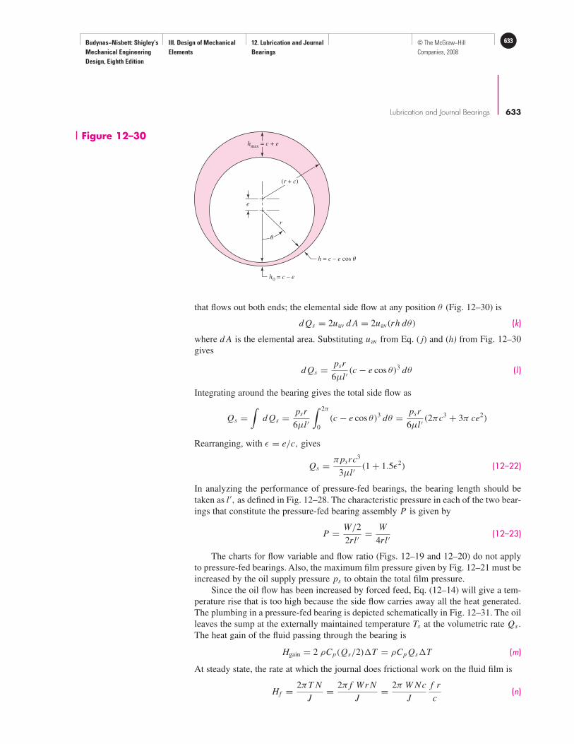
Budynas−Nisbett: Shigley’s
Mechanical Engineering
Design, Eighth Edition
III. Design of Mechanical
Elements
12. Lubrication and Journal
Bearings
633© The McGraw−Hill
Companies, 2008
Lubrication and Journal Bearings 633
e
r
(r + c)
h = c – e cos
h0 = c – e
hmax = c + eFigure 12–30
that flows out both ends; the elemental side flow at any position θ (Fig. 12–30) is
d Qs = 2uav d A = 2uav(rh dθ) (k)
where d A is the elemental area. Substituting uav from Eq. ( j) and (h) from Fig. 12–30
gives
d Qs = psr
6µl ′(c − e cos θ)3 dθ (l )
Integrating around the bearing gives the total side flow as
Qs =∫
d Qs = psr
6µl ′
∫ 2π
0
(c − e cos θ)3 dθ = psr
6µl ′(2πc3 + 3π ce2)
Rearranging, with ε = e/c, gives
Qs = πpsrc3
3µl ′(1 + 1.5ε2) (12–22)
In analyzing the performance of pressure-fed bearings, the bearing length should be
taken as l ′, as defined in Fig. 12–28. The characteristic pressure in each of the two bear-
ings that constitute the pressure-fed bearing assembly P is given by
P = W/2
2rl ′= W
4rl ′(12–23)
The charts for flow variable and flow ratio (Figs. 12–19 and 12–20) do not apply
to pressure-fed bearings. Also, the maximum film pressure given by Fig. 12–21 must be
increased by the oil supply pressure ps to obtain the total film pressure.
Since the oil flow has been increased by forced feed, Eq. (12–14) will give a tem-
perature rise that is too high because the side flow carries away all the heat generated.
The plumbing in a pressure-fed bearing is depicted schematically in Fig. 12–31. The oil
leaves the sump at the externally maintained temperature Ts at the volumetric rate Qs .
The heat gain of the fluid passing through the bearing is
Hgain = 2 ρCp(Qs/2)�T = ρCp Qs�T (m)
At steady state, the rate at which the journal does frictional work on the fluid film is
Hf = 2πT N
J= 2π f Wr N
J= 2π W Nc
J
f r
c(n)
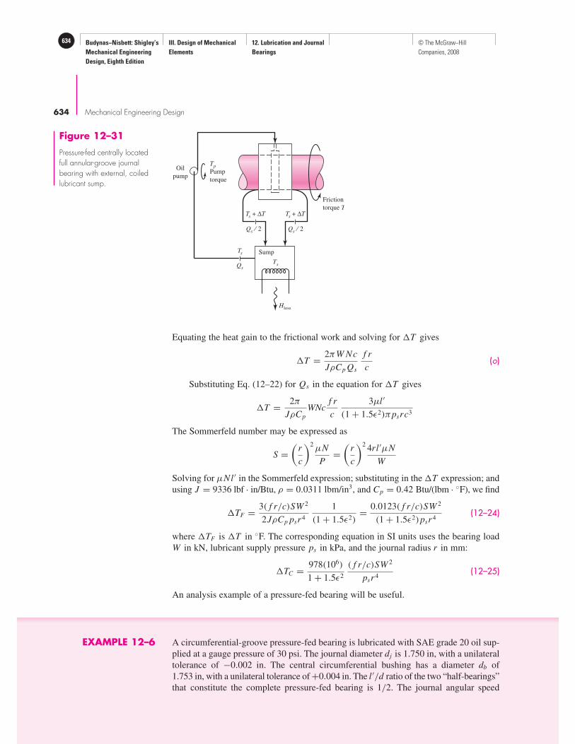
Budynas−Nisbett: Shigley’s
Mechanical Engineering
Design, Eighth Edition
III. Design of Mechanical
Elements
12. Lubrication and Journal
Bearings
634 © The McGraw−Hill
Companies, 2008
634 Mechanical Engineering Design
Equating the heat gain to the frictional work and solving for �T gives
�T = 2πW Nc
JρCp Qs
f r
c(o)
Substituting Eq. (12–22) for Qs in the equation for �T gives
�T = 2π
JρCp
WNcf r
c
3µl ′
(1 + 1.5ε2)πpsrc3
The Sommerfeld number may be expressed as
S =(
r
c
)2µN
P=(
r
c
)24rl ′µN
W
Solving for µNl ′ in the Sommerfeld expression; substituting in the �T expression; and
using J = 9336 lbf · in/Btu, ρ = 0.0311 lbm/in3, and Cp = 0.42 Btu/(lbm · ◦F), we find
�TF = 3( f r/c)SW 2
2JρCp psr4
1
(1 + 1.5ε2)= 0.0123( f r/c)SW 2
(1 + 1.5ε2)psr4(12–24)
where �TF is �T in ◦F. The corresponding equation in SI units uses the bearing load
W in kN, lubricant supply pressure ps in kPa, and the journal radius r in mm:
�TC = 978(106)
1 + 1.5ε2
( f r/c)SW 2
psr4(12–25)
An analysis example of a pressure-fed bearing will be useful.
EXAMPLE 12–6 A circumferential-groove pressure-fed bearing is lubricated with SAE grade 20 oil sup-
plied at a gauge pressure of 30 psi. The journal diameter dj is 1.750 in, with a unilateral
tolerance of −0.002 in. The central circumferential bushing has a diameter db of
1.753 in, with a unilateral tolerance of +0.004 in. The l ′/d ratio of the two “half-bearings”
that constitute the complete pressure-fed bearing is 1/2. The journal angular speed
Oil
pump
Tp
Pump
torque
Friction
torque T
Sump
Ts
Ts + ∆T Ts + ∆T
Qs ⁄ 2 Qs ⁄ 2
Hloss
Ts
Qs
Figure 12–31
Pressure-fed centrally locatedfull annular-groove journalbearing with external, coiledlubricant sump.
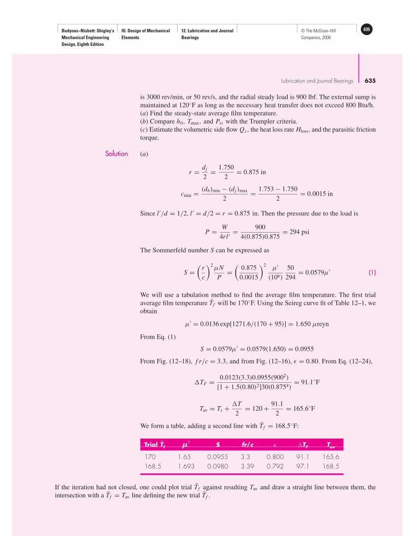
Budynas−Nisbett: Shigley’s
Mechanical Engineering
Design, Eighth Edition
III. Design of Mechanical
Elements
12. Lubrication and Journal
Bearings
635© The McGraw−Hill
Companies, 2008
Lubrication and Journal Bearings 635
is 3000 rev/min, or 50 rev/s, and the radial steady load is 900 lbf. The external sump is
maintained at 120◦F as long as the necessary heat transfer does not exceed 800 Btu/h.
(a) Find the steady-state average film temperature.
(b) Compare h0, Tmax, and Pst with the Trumpler criteria.
(c) Estimate the volumetric side flow Qs, the heat loss rate Hloss, and the parasitic friction
torque.
Solution (a)
r = dj
2= 1.750
2= 0.875 in
cmin = (db)min − (dj )max
2= 1.753 − 1.750
2= 0.0015 in
Since l ′/d = 1/2, l ′ = d/2 = r = 0.875 in. Then the pressure due to the load is
P = W
4rl ′= 900
4(0.875)0.875= 294 psi
The Sommerfeld number S can be expressed as
S =(
r
c
)2µN
P=(
0.875
0.0015
)2µ′
(106)
50
294= 0.0579µ′ (1)
We will use a tabulation method to find the average film temperature. The first trial
average film temperature Tf will be 170◦F. Using the Seireg curve fit of Table 12–1, we
obtain
µ′ = 0.0136 exp[1271.6/(170 + 95)] = 1.650 µreyn
From Eq. (1)
S = 0.0579µ′ = 0.0579(1.650) = 0.0955
From Fig. (12–18), f r/c = 3.3, and from Fig. (12–16), ε = 0.80. From Eq. (12–24),
�TF = 0.0123(3.3)0.0955(9002)
[1 + 1.5(0.80)2]30(0.8754)= 91.1◦F
Tav = Ts + �T
2= 120 + 91.1
2= 165.6◦F
We form a table, adding a second line with Tf = 168.5◦F:
If the iteration had not closed, one could plot trial Tf against resulting Tav and draw a straight line between them, the
intersection with a Tf = Tav line defining the new trial Tf .
Trial Tf � S fr/c ε �
170 1.65 0.0955 3.3 0.800 91.1 165.6
168.5 1.693 0.0980 3.39 0.792 97.1 168.5
TF Tav
Budynas−Nisbett: Shigley’s
Mechanical Engineering
Design, Eighth Edition
III. Design of Mechanical
Elements
12. Lubrication and Journal
Bearings
636 © The McGraw−Hill
Companies, 2008
636 Mechanical Engineering Design
Answer The result of this tabulation is Tf = 168.5, �TF = 97.1◦F, and Tmax = 120 + 97.1 =217.1◦F
(b) Since h0 = (1 − ε)c,
h0 = (1 − 0.792)0.0015 = 0.000 312 in
The required four Trumpler criteria, from “Significant Angular Speed” in Sec. 12–7 are
h0 ≥ 0.0002 + 0.000 04(1.750) = 0.000 270 in (OK)
Answer Tmax = Ts + �T = 120 + 97.1 = 217.1◦F (OK)
Pst = Wst
4rl ′= 900
4(0.875)0.875= 294 psi (OK)
The factor of safety on the load is approximately unity. (Not OK.)
(c) From Eq. (12–22),
Answer Qs = π(30)0.875(0.0015)3
3(1.693)10−6(0.875)[1 + 1.5(0.80)2] = 0.123 in3/s
Hloss = ρCp Qs�T = 0.0311(0.42)0.123(97.1) = 0.156 Btu/s
or 562 Btu/h or 0.221 hp. The parasitic friction torque T is
Answer T = f Wr = f r
cWc = 3.39(900)0.0015 = 4.58 lbf · in
12–12 Loads and MaterialsSome help in choosing unit loads and bearing materials is afforded by Tables 12–5 and
12–6. Since the diameter and length of a bearing depend upon the unit load, these tables
will help the designer to establish a starting point in the design.
Unit Load
Application psi MPa
Diesel engines:Main bearings 900–1700 6–12Crankpin 1150–2300 8–15Wristpin 2000–2300 14–15
Electric motors 120–250 0.8–1.5
Steam turbines 120–250 0.8–1.5
Gear reducers 120–250 0.8–1.5
Automotive engines:Main bearings 600–750 4–5Crankpin 1700–2300 10–15
Air compressors:Main bearings 140–280 1–2Crankpin 280–500 2–4
Centrifugal pumps 100–180 0.6–1.2
Table 12–5
Range of Unit Loads in
Current Use for Sleeve
Bearings

Budynas−Nisbett: Shigley’s
Mechanical Engineering
Design, Eighth Edition
III. Design of Mechanical
Elements
12. Lubrication and Journal
Bearings
637© The McGraw−Hill
Companies, 2008
Lubrication and Journal Bearings 637
Thickness, SAE Clearance Load CorrosionAlloy Name in Number Ratio r/c Capacity Resistance
Tin-base babbitt 0.022 12 600–1000 1.0 Excellent
Lead-base babbitt 0.022 15 600–1000 1.2 Very good
Tin-base babbitt 0.004 12 600–1000 1.5 Excellent
Lead-base babbitt 0.004 15 600–1000 1.5 Very good
Leaded bronze Solid 792 500–1000 3.3 Very good
Copper-lead 0.022 480 500–1000 1.9 Good
Aluminum alloy Solid 400–500 3.0 Excellent
Silver plus overlay 0.013 17P 600–1000 4.1 Excellent
Cadmium (1.5% Ni) 0.022 18 400–500 1.3 Good
Trimetal 88* 4.1 Excellent
Trimetal 77† 4.1 Very good
*This is a 0.008-in layer of copper-lead on a steel back plus 0.001 in of tin-base babbitt.†This is a 0.013-in layer of copper-lead on a steel back plus 0.001 in of lead-base babbitt.
Table 12–6
Some Characteristics
of Bearing Alloys
The length-diameter ratio l/d of a bearing depends upon whether it is expected to
run under thin-film-lubrication conditions. A long bearing (large l/d ratio) reduces the
coefficient of friction and the side flow of oil and therefore is desirable where thin-film
or boundary-value lubrication is present. On the other hand, where forced-feed or pos-
itive lubrication is present, the l/d ratio should be relatively small. The short bearing
length results in a greater flow of oil out of the ends, thus keeping the bearing cooler.
Current practice is to use an l/d ratio of about unity, in general, and then to increase
this ratio if thin-film lubrication is likely to occur and to decrease it for thick-film lubri-
cation or high temperatures. If shaft deflection is likely to be severe, a short bearing
should be used to prevent metal-to-metal contact at the ends of the bearings.
You should always consider the use of a partial bearing if high temperatures are a
problem, because relieving the non-load-bearing area of a bearing can very substantially
reduce the heat generated.
The two conflicting requirements of a good bearing material are that it must have a
satisfactory compressive and fatigue strength to resist the externally applied loads and
that it must be soft and have a low melting point and a low modulus of elasticity. The
second set of requirements is necessary to permit the material to wear or break in, since
the material can then conform to slight irregularities and absorb and release foreign par-
ticles. The resistance to wear and the coefficient of friction are also important because all
bearings must operate, at least for part of the time, with thin-film or boundary lubrication.
Additional considerations in the selection of a good bearing material are its ability
to resist corrosion and, of course, the cost of producing the bearing. Some of the com-
monly used materials are listed in Table 12–6, together with their composition and
characteristics.
Bearing life can be increased very substantially by depositing a layer of babbitt, or
other white metal, in thicknesses from 0.001 to 0.014 in over steel backup material. In
fact, a copper-lead layer on steel to provide strength, combined with a babbitt overlay to
enhance surface conformability and corrosion resistance, makes an excellent bearing.
Small bushings and thrust collars are often expected to run with thin-film or bound-
ary lubrication. When this is the case, improvements over a solid bearing material can
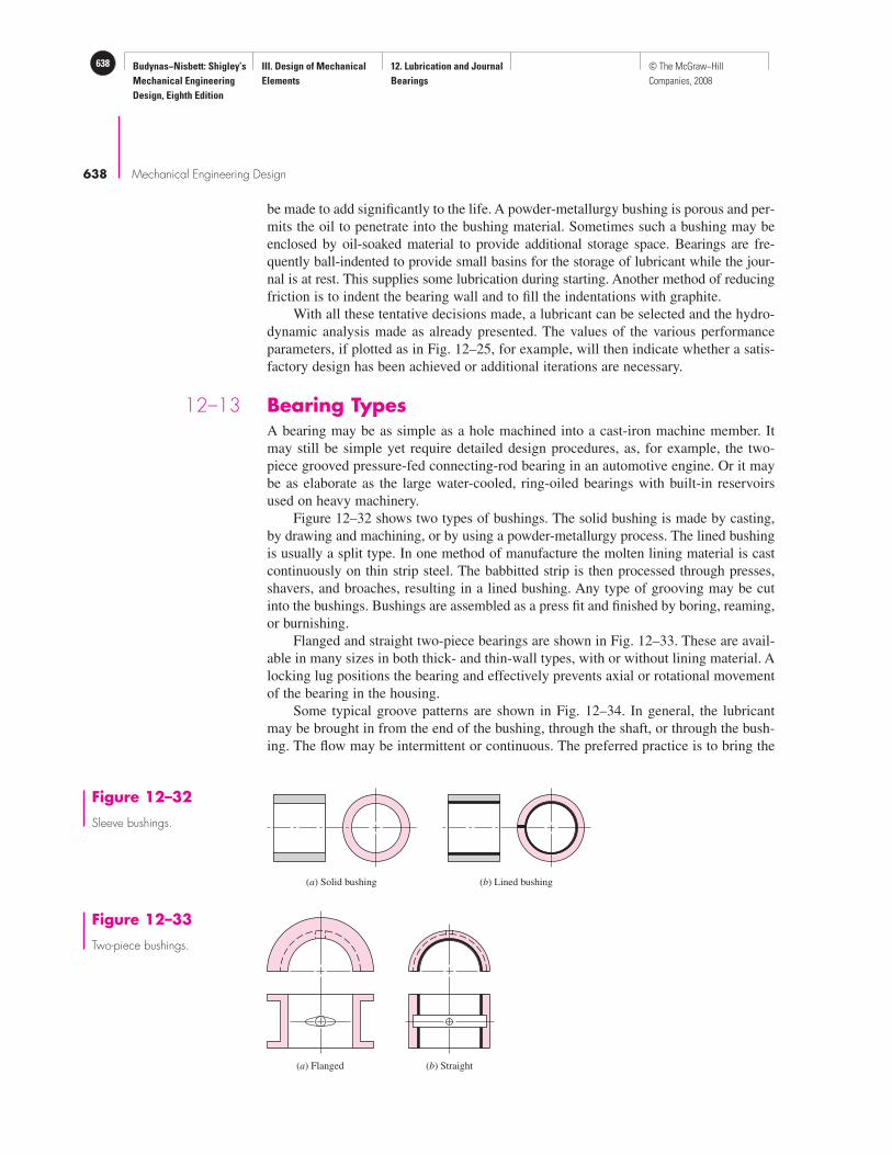
Budynas−Nisbett: Shigley’s
Mechanical Engineering
Design, Eighth Edition
III. Design of Mechanical
Elements
12. Lubrication and Journal
Bearings
638 © The McGraw−Hill
Companies, 2008
638 Mechanical Engineering Design
be made to add significantly to the life. A powder-metallurgy bushing is porous and per-
mits the oil to penetrate into the bushing material. Sometimes such a bushing may be
enclosed by oil-soaked material to provide additional storage space. Bearings are fre-
quently ball-indented to provide small basins for the storage of lubricant while the jour-
nal is at rest. This supplies some lubrication during starting. Another method of reducing
friction is to indent the bearing wall and to fill the indentations with graphite.
With all these tentative decisions made, a lubricant can be selected and the hydro-
dynamic analysis made as already presented. The values of the various performance
parameters, if plotted as in Fig. 12–25, for example, will then indicate whether a satis-
factory design has been achieved or additional iterations are necessary.
12–13 Bearing TypesA bearing may be as simple as a hole machined into a cast-iron machine member. It
may still be simple yet require detailed design procedures, as, for example, the two-
piece grooved pressure-fed connecting-rod bearing in an automotive engine. Or it may
be as elaborate as the large water-cooled, ring-oiled bearings with built-in reservoirs
used on heavy machinery.
Figure 12–32 shows two types of bushings. The solid bushing is made by casting,
by drawing and machining, or by using a powder-metallurgy process. The lined bushing
is usually a split type. In one method of manufacture the molten lining material is cast
continuously on thin strip steel. The babbitted strip is then processed through presses,
shavers, and broaches, resulting in a lined bushing. Any type of grooving may be cut
into the bushings. Bushings are assembled as a press fit and finished by boring, reaming,
or burnishing.
Flanged and straight two-piece bearings are shown in Fig. 12–33. These are avail-
able in many sizes in both thick- and thin-wall types, with or without lining material. A
locking lug positions the bearing and effectively prevents axial or rotational movement
of the bearing in the housing.
Some typical groove patterns are shown in Fig. 12–34. In general, the lubricant
may be brought in from the end of the bushing, through the shaft, or through the bush-
ing. The flow may be intermittent or continuous. The preferred practice is to bring the
(a) Solid bushing (b) Lined bushing
Figure 12–32
Sleeve bushings.
(a) Flanged (b) Straight
Figure 12–33
Two-piece bushings.
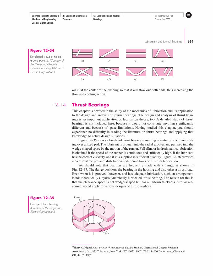
Budynas−Nisbett: Shigley’s
Mechanical Engineering
Design, Eighth Edition
III. Design of Mechanical
Elements
12. Lubrication and Journal
Bearings
639© The McGraw−Hill
Companies, 2008
Lubrication and Journal Bearings 639
Pads
Runner
R2
NR1
Figure 12–35
Fixed-pad thrust bearing.(Courtesy of WestinghouseElectric Corporation.)
oil in at the center of the bushing so that it will flow out both ends, thus increasing the
flow and cooling action.
12–14 Thrust BearingsThis chapter is devoted to the study of the mechanics of lubrication and its application
to the design and analysis of journal bearings. The design and analysis of thrust bear-
ings is an important application of lubrication theory, too. A detailed study of thrust
bearings is not included here, because it would not contribute anything significantly
different and because of space limitations. Having studied this chapter, you should
experience no difficulty in reading the literature on thrust bearings and applying that
knowledge to actual design situations.11
Figure 12–35 shows a fixed-pad thrust bearing consisting essentially of a runner slid-
ing over a fixed pad. The lubricant is brought into the radial grooves and pumped into the
wedge-shaped space by the motion of the runner. Full-film, or hydrodynamic, lubrication
is obtained if the speed of the runner is continuous and sufficiently high, if the lubricant
has the correct viscosity, and if it is supplied in sufficient quantity. Figure 12–36 provides
a picture of the pressure distribution under conditions of full-film lubrication.
We should note that bearings are frequently made with a flange, as shown in
Fig. 12–37. The flange positions the bearing in the housing and also takes a thrust load.
Even when it is grooved, however, and has adequate lubrication, such an arrangement
is not theoretically a hydrodynamically lubricated thrust bearing. The reason for this is
that the clearance space is not wedge-shaped but has a uniform thickness. Similar rea-
soning would apply to various designs of thrust washers.
(a)
(e)
(b)
( f )
(c)
(g)
(d )
(h)
Figure 12–34
Developed views of typicalgroove patterns. (Courtesy ofthe Cleveland GraphiteBronze Company, Division ofClevite Corporation.)
11Harry C. Rippel, Cast Bronze Thrust Bearing Design Manual, International Copper Research
Association, Inc., 825 Third Ave., New York, NY 10022, 1967. CBBI, 14600 Detroit Ave., Cleveland,
OH, 44107, 1967.

Budynas−Nisbett: Shigley’s
Mechanical Engineering
Design, Eighth Edition
III. Design of Mechanical
Elements
12. Lubrication and Journal
Bearings
640 © The McGraw−Hill
Companies, 2008
640 Mechanical Engineering Design
12–15 Boundary-Lubricated BearingsWhen two surfaces slide relative to each other with only a partial lubricant film between
them, boundary lubrication is said to exist. Boundary- or thin-film lubrication occurs in
hydrodynamically lubricated bearings when they are starting or stopping, when the load
increases, when the supply of lubricant decreases, or whenever other operating changes
happen to occur. There are, of course, a very large number of cases in design in which
boundary-lubricated bearings must be used because of the type of application or the
competitive situation.
The coefficient of friction for boundary-lubricated surfaces may be greatly
decreased by the use of animal or vegetable oils mixed with the mineral oil or grease.
Fatty acids, such as stearic acid, palmitic acid, or oleic acid, or several of these, which
occur in animal and vegetable fats, are called oiliness agents. These acids appear to
reduce friction, either because of their strong affinity for certain metallic surfaces or
because they form a soap film that binds itself to the metallic surfaces by a chemical
reaction. Thus the fatty-acid molecules bind themselves to the journal and bearing sur-
faces with such great strength that the metallic asperities of the rubbing metals do not
weld or shear.
Fatty acids will break down at temperatures of 250◦F or more, causing increased
friction and wear in thin-film-lubricated bearings. In such cases the extreme-pressure,
or EP, lubricants may be mixed with the fatty-acid lubricant. These are composed of
chemicals such as chlorinated esters or tricresyl phosphate, which form an organic film
between the rubbing surfaces. Though the EP lubricants make it possible to operate at
higher temperatures, there is the added possibility of excessive chemical corrosion of
the sliding surfaces.
When a bearing operates partly under hydrodynamic conditions and partly under
dry or thin-film conditions, a mixed-film lubrication exists. If the lubricant is supplied by
hand oiling, by drop or mechanical feed, or by wick feed, for example, the bearing is
U
h
Runner
Thrustbearingpad
Pressure distributionFigure 12–36
Pressure distribution oflubricant in a thrust bearing.(Courtesy of Copper ResearchCorporation.)
Figure 12–37
Flanged sleeve bearing takesboth radial and thrust loads.

Budynas−Nisbett: Shigley’s
Mechanical Engineering
Design, Eighth Edition
III. Design of Mechanical
Elements
12. Lubrication and Journal
Bearings
641© The McGraw−Hill
Companies, 2008
Lubrication and Journal Bearings 641
Maximum Maximum Maximum MaximumLoad, Temperature, Speed, PV
Material psi °F fpm Value*
Cast bronze 4 500 325 1 500 50 000
Porous bronze 4 500 150 1 500 50 000
Porous iron 8 000 150 800 50 000
Phenolics 6 000 200 2 500 15 000
Nylon 1 000 200 1 000 3 000
Teflon 500 500 100 1 000
Reinforced Teflon 2 500 500 1 000 10 000
Teflon fabric 60 000 500 50 25 000
Delrin 1 000 180 1 000 3 000
Carbon-graphite 600 750 2 500 15 000
Rubber 50 150 4 000
Wood 2 000 150 2 000 15 000
*P � load, psi; V � speed, fpm.
Table 12–7
Some Materials for
Boundary-Lubricated
Bearings and Their
Operating Limits
operating under mixed-film conditions. In addition to occurring with a scarcity of lubri-
cant, mixed-film conditions may be present when
• The viscosity is too low.
• The bearing speed is too low.
• The bearing is overloaded.
• The clearance is too tight.
• Journal and bearing are not properly aligned.
Relative motion between surfaces in contact in the presence of a lubricant is called
boundary lubrication. This condition is present in hydrodynamic film bearings during
starting, stopping, overloading, or lubricant deficiency. Some bearings are boundary
lubricated (or dry) at all times. To signal this an adjective is placed before the word
“bearing.” Commonly applied adjectives (to name a few) are thin-film, boundary fric-
tion, Oilite, Oiles, and bushed-pin. The applications include situations in which thick
film will not develop and there are low journal speed, oscillating journal, padded slides,
light loads, and lifetime lubrication. The characteristics include considerable friction,
ability to tolerate expected wear without losing function, and light loading. Such bear-
ings are limited by lubricant temperature, speed, pressure, galling, and cumulative wear.
Table 12–7 gives some properties of a range of bushing materials.
Linear Sliding Wear
Consider the sliding block depicted in Fig. 12–38, moving along a plate with contact
pressure P ′ acting over area A, in the presence of a coefficient of sliding friction fs . The
linear measure of wear w is expressed in inches or millimeters. The work done by force
fs P A during displacement S is fs P AS or fs P AV t , where V is the sliding velocity and
t is time. The material volume removed due to wear is wA and is proportional to the
work done, that is, wA ∝ fs P AV t , or
wA = K P AV t

Budynas−Nisbett: Shigley’s
Mechanical Engineering
Design, Eighth Edition
III. Design of Mechanical
Elements
12. Lubrication and Journal
Bearings
642 © The McGraw−Hill
Companies, 2008
642 Mechanical Engineering Design
where K is the proportionality factor, which includes fs , and is determined from labo-
ratory testing. The linear wear is then expressed as
w = K PV t (12–26)
In US customary units, P is expressed in psi, V in fpm (i.e., ft/min), and t in hours.
This makes the units of K in3 · min/(lbf · ft · h). SI units commonly used for K are
cm3 · min/(kgf · m · h), where 1 kgf = 9.806 N. Tables 12–8 and 12–9 give some wear
factors and coefficients of friction from one manufacturer.
F F
w
PAPA
fsPAfsPA
S
A �A�A
Figure 12–38
Sliding block subjectedto wear.
Table 12–8
Wear Factors in U.S.
Customary Units*
Source: Oiles America Corp.,Plymouth, MI 48170.
Bushing Wear Factor LimitingMaterial K PV
Oiles 800 3(10−10 ) 18 000
Oiles 500 0.6(10−10 ) 46 700
Polyactal copolymer 50(10−10 ) 5 000
Polyactal homopolymer 60(10−10 ) 3 000
66 nylon 200(10−10 ) 2 000
66 nylon + 15% PTFE 13(10−10 ) 7 000
+ 15% PTFE + 30% glass 16(10−10 ) 10 000
+ 2.5% MoS2 200(10−10 ) 2 000
6 nylon 200(10−10 ) 2 000
Polycarbonate + 15% PTFE 75(10−10 ) 7 000
Sintered bronze 102(10−10 ) 8 500
Phenol + 25% glass fiber 8(10−10 ) 11 500
*dim[K ] � in3 · min/(lbf · ft · h), dim [PV] � psi · ft/min.
Type Bearing fs
Placetic Oiles 80 0.05
Composite Drymet ST 0.03Toughmet 0.05
Met Cermet M 0.05Oiles 2000 0.03Oiles 300 0.03Oiles 500SP 0.03
Table 12–9
Coefficients of Friction
Source: Oiles America Corp.,Plymouth, MI 48170.

Budynas−Nisbett: Shigley’s
Mechanical Engineering
Design, Eighth Edition
III. Design of Mechanical
Elements
12. Lubrication and Journal
Bearings
643© The McGraw−Hill
Companies, 2008
Lubrication and Journal Bearings 643
Characteristic Velocity V,Mode of Motion Pressure P, psi ft/min f1*
Rotary 720 or less 3.3 or less 1.03.3–33 1.0–1.333–100 1.3–1.8
720–3600 3.3 or less 1.53.3–33 1.5–2.033–100 2.0–2.7
Oscillatory 720 or less >30◦ 3.3 or less 1.33.3–100 1.3–2.4
<30◦ 3.3 or less 2.03.3–100 2.0–3.6
720–3600 >30◦ 3.3 or less 2.03.3–100 2.0–3.2
<30◦ 3.3 or less 3.03.3–100 3.0–4.8
Reciprocating 720 or less 33 or less 1.533–100 1.5–3.8
720–3600 33 or less 2.033–100 2.0–7.5
*Values of f1 based on results over an extended period of time on automotive manufacturing machinery.
Table 12–10
Motion-Related Factor f1
Ambient Temperature, °F Foreign Matter f2
140 or lower No 1.0
140 or lower Yes 3.0–6.0
140–210 No 3.0–6.0
140–210 Yes 6.0–12.0
Table 12–11
Environmental Factor f2Source: Oiles America Corp.,Plymouth, MI 48170.
It is useful to include a modifying factor f1 depending on motion type, load, and
speed and an environment factor f2 to account for temperature and cleanliness conditions
(see Tables 12–10 and 12–11). These factors account for departures from the laboratory
conditions under which K was measured. Equation (12–26) can now be written as
w = f1 f2 K PV t (12–27)
Wear, then, is proportional to PV , material property K, operating conditions f1 and f2,
and time t.
Bushing Wear
Consider a pin of diameter D, rotating at speed N, in a bushing of length L, and sup-
porting a stationary radial load F. The nominal pressure P is given by
P = F
DL(12–28)

Budynas−Nisbett: Shigley’s
Mechanical Engineering
Design, Eighth Edition
III. Design of Mechanical
Elements
12. Lubrication and Journal
Bearings
644 © The McGraw−Hill
Companies, 2008
644 Mechanical Engineering Design
and if N is in rev/min and D is in inches, velocity in ft/min is given by
V = π DN
12(12–29)
Thus PV , in psi · ft/min, is
PV = F
DL
π DN
12= π
12
FN
L(12–30)
Note the independence of PV from the journal diameter D.
A time-wear equation similar to Eq. (12–27) can be written. However, before do-
ing so, it is important to note that Eq. (12–28) provides the nominal value of P.
Figure 12–39 provides a more accurate representation of the pressure distribution,
which can be written as
p = Pmax cos θ −π
2≤ θ ≤ π
2
The vertical component of p d A is p d A cos θ = [pL(D/2) dθ] cos θ = Pmax(DL/2)
cos2 θ dθ . Integrating this from θ = −π/2 to π/2 yields F. Thus,
∫ π/2
−π/2
Pmax
(
DL
2
)
cos2 θ dθ = π
4Pmax DL = F
or
Pmax = 4
π
F
DL(12–31)
Substituting V from Eq. (12–29) and Pmax for P from Eq. (12–31) into Eq. (12–27) gives
w = f1 f2 K4
π
F
DL
π DN t
12= f1 f2 K F N t
3L(12–32)
In designing a bushing, because of various trade-offs it is recommended that the
length/diameter ratio be in the range
0.5 ≤ L/D ≤ 2 (12–33)
F
Pmax
P
D�2
Figure 12–39
Pressure distribution on aboundary-lubricated bushing.

Budynas−Nisbett: Shigley’s
Mechanical Engineering
Design, Eighth Edition
III. Design of Mechanical
Elements
12. Lubrication and Journal
Bearings
645© The McGraw−Hill
Companies, 2008
Lubrication and Journal Bearings 645
1 in
1 in
700 lbf
Figure 12–40
Journal/bushing for Ex. 12–7.
Service Range Units Allowable
Characteristic pressure Pmax psi <3560
Velocity Vmax ft/min <100
PV product (psi)(ft/min) <46 700
Temperature T °F <300
Properties Test Method, Units Value
Tensile strength (ASTM E8) psi >110 000
Elongation (ASTM E8) % >12
Compressive strength (ASTM E9) psi 49 770
Brinell hardness (ASTM E10) HB >210
Coefficient of thermal (10−5 ) °C >1.6expansion
Specific gravity 8.2
Table 12–12
Oiles 500 SP (SPBN ·
SPWN) Service Range
and Properties
Source: Oiles America Corp.,Plymouth, MI 48170.
EXAMPLE 12–7 An Oiles SP 500 alloy brass bushing is 1 in long with a 1-in bore and operates in a clean
environment at 70◦F. The allowable wear without loss of function is 0.005 in. The radial
load is 700 lbf. The peripheral velocity is 33 ft/min. Estimate the number of revolutions
for radial wear to be 0.005 in. See Fig. 12–40 and Table 12–12 from the manufacturer.
Solution From Table 12–8, K = 0.6(10−10) in3 · min/(lbf · ft · h); Tables 12–10 and 12–11, f1 =1.3, f2 = 1; and Table 12–12, PV = 46 700 psi · ft/min, Pmax = 3560 psi, Vmax =100 ft/min. From Eqs. (12–31), (12–29), and (12–30),
Pmax = 4
π
F
DL= 4
π
700
(1)(1)= 891 psi < 3560 psi (OK)
P = F
DL= 700
(1)(1)= 700 psi
V = 33 ft/min < 100 ft/min (OK)
PV = 700(33) = 23 100 psi · ft/min < 46 700 psi · ft/min (OK)
Equation (12–32) with Eq. (12–29) is
w = f1 f2 K4
π
F
DL
π DN t
12= f1 f2 K
4
π
F
DLV t

Budynas−Nisbett: Shigley’s
Mechanical Engineering
Design, Eighth Edition
III. Design of Mechanical
Elements
12. Lubrication and Journal
Bearings
646 © The McGraw−Hill
Companies, 2008
646 Mechanical Engineering Design
Solving for t gives
t = π DLw
4 f1 f2 K V F= π(1)(1)0.005
4(1.3)(1)0.6(10−10)33(700)= 2180 h = 130 770 min
The rotational speed is
N = 12V
π D= 12(33)
π(1)= 126 r/min
Answer Cycles = Nt = 126(130 770) = 16.5(106) rev
Temperature Rise
At steady state, the rate at which work is done against bearing friction equals the rate
at which heat is transferred from the bearing housing to the surroundings by convection
and radiation. The rate of heat generation in Btu/h is given by fs FV /J , or
Hgen = fs F(π D)(60N )
12J= 5π fs F DN
J(12–34)
where N is journal speed in rev/min and J = 778 ft · lbf/Btu. The rate at which heat is
transferred to the surroundings, in Btu/h, is
Hloss = hCR A�T = hCR A(Tb − T∞) = hCR A
2(Tf − T∞) (12–35)
where A = housing surface area, ft2
hCR = overall combined coefficient of heat transfer, Btu/(h · ft2 · ◦F)
Tb = housing metal temperature, ◦F
Tf = lubricant temperature, ◦F
The empirical observation that Tb is about midway between Tf and T∞ has been incor-
porated in Eq. (12–35). Equating Eqs. (12–34) and (12–35) gives
Tf = T∞ + 10π fs F DN
JhCR A(12–36)
Although this equation seems to indicate the temperature rise Tf − T∞ is independent
of length L, the housing surface area generally is a function of L. The housing surface
area can be initially estimated, and as tuning of the design proceeds, improved results
will converge. If the bushing is to be housed in a pillow block, the surface area can be
roughly estimated from
A.= 2π DL
144(12–37)
Substituting Eq. (12–37) into Eq. (12–36) gives
Tf.= T∞ + 10π fs F DN
JhCR(2π DL/144)= T∞ + 720 fs F N
JhCRL(12–38)
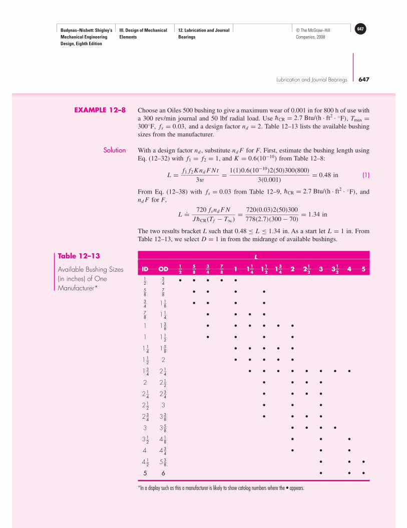
Budynas−Nisbett: Shigley’s
Mechanical Engineering
Design, Eighth Edition
III. Design of Mechanical
Elements
12. Lubrication and Journal
Bearings
647© The McGraw−Hill
Companies, 2008
Lubrication and Journal Bearings 647
L
ID OD 1 1 1 1 2 2 3 3 4 5
12
34
• • • • •
58
78
• • • •
34
1 18
• • • •
78
1 14
• • • •
1 1 38
• • • • • •
1 1 12
• • • •
1 14
1 58
• • • • •
1 12
2 • • • • •
1 34
2 14
• • • • • • • •
2 2 12
• • • •
2 14
2 34
• • • •
2 12
3 • • •
2 34
3 38
• • • •
3 3 58
• • • •
3 12
4 18
• • •
4 4 34
• • •
4 12
5 38
• • •
5 6 • • •
*In a display such as this a manufacturer is likely to show catolog numbers where the • appears.
1
2
1
2
3
4
1
2
1
4
7
8
3
4
5
8
1
2
Table 12–13
Available Bushing Sizes
(in inches) of One
Manufacturer*
EXAMPLE 12–8 Choose an Oiles 500 bushing to give a maximum wear of 0.001 in for 800 h of use with
a 300 rev/min journal and 50 lbf radial load. Use hCR = 2.7 Btu/(h · ft2 · ◦F), Tmax =300◦F, fs = 0.03, and a design factor nd = 2. Table 12–13 lists the available bushing
sizes from the manufacturer.
Solution With a design factor nd , substitute nd F for F. First, estimate the bushing length using
Eq. (12–32) with f1 = f2 = 1, and K = 0.6(10−10) from Table 12–8:
L = f1 f2 K nd F Nt
3w= 1(1)0.6(10−10)2(50)300(800)
3(0.001)= 0.48 in (1)
From Eq. (12–38) with fs = 0.03 from Table 12–9, hCR = 2.7 Btu/(h · ft2 · ◦F), and
nd F for F,
L.= 720 fsnd F N
JhCR(Tf − T∞)= 720(0.03)2(50)300
778(2.7)(300 − 70)= 1.34 in
The two results bracket L such that 0.48 ≤ L ≤ 1.34 in. As a start let L = 1 in. From
Table 12–13, we select D = 1 in from the midrange of available bushings.

Budynas−Nisbett: Shigley’s
Mechanical Engineering
Design, Eighth Edition
III. Design of Mechanical
Elements
12. Lubrication and Journal
Bearings
648 © The McGraw−Hill
Companies, 2008
648 Mechanical Engineering Design
Trial 1: D = L = 1 in.
Eq. (12–31): Pmax = 4
π
nd F
DL= 4
π
2(50)
1(1)= 127 psi < 3560 psi (OK)
P = nd F
DL= 2(50)
1(1)= 100 psi
Eq. (12–29): V = π DN
12= π(1)300
12= 78.5 ft/min < 100 ft/min (OK)
PV = 100(78.5) = 7850 psi · ft/min < 46 700 psi · ft/min (OK)
From Table 12–9,
Our second estimate is L ≥ 0.48(1.64) = 0.787 in. From Table 12–13, there is not
much available for L = 78
in. So staying with L = 1 in, try D = 12
in.
Trial 2: D = 0.5 in, L = 1 in.
Pmax = 4
π
nd F
DL= 4
π
2(50)
0.5(1)= 255 psi < 3560 psi (OK)
P = nd F
DL= 2(50)
0.5(1)= 200 psi
V = π DN
12= π(0.5)300
12= 39.3 ft /min < 100 ft /min (OK)
Note that PV is not a function of D, and since we did not change L, PV will remain
the same:
PV = 200(39.3) = 7860 psi · ft/min < 46 700 psi · ft/min (OK)
From Table 12–9, f1 = 1.34, L ≥ 1.34(0.48) = 0.643 in. There are many 34-in bush-
ings to select from. The smallest diameter in Table 12–13 is D = 12
in. This gives an
L/D ratio of 1.5, which is acceptable according to Eq. (12–33).
Trial 3: D = 0.5 in, L = 0.75 in. From trial 2, V = 39.3 ft/min does not change.
Pmax = 4
π
nd F
DL= 4
π
2(50)
0.5(0.75)= 340 psi < 3560 psi (OK)
P = nd F
DL= 2(50)
0.5(0.75)= 267 psi
PV = 267(39.3) = 10 490 psi · ft /min < 46 700 psi · ft /min (OK)
Answer Select any of the bushings from the trials, where the optimum, from trial 3, is D = 12
in
and L = 34
in. Other factors may enter in the overall design that make the other bushings
more appropriate.
V f1
33 1.3
78.5 f1 �� f1 � 1.64
100 1.8

Budynas−Nisbett: Shigley’s
Mechanical Engineering
Design, Eighth Edition
III. Design of Mechanical
Elements
12. Lubrication and Journal
Bearings
649© The McGraw−Hill
Companies, 2008
Lubrication and Journal Bearings 649
PROBLEMS
12–1 A full journal bearing has a journal diameter of 1.000 in, with a unilateral tolerance of
−0.0015 in. The bushing bore has a diameter of 1.0015 in and a unilateral tolerance of 0.003 in.
The l/d ratio is unity. The load is 250 lbf and the journal runs at 1100 rev/min. If the average vis-
cosity is 8 µreyn, find the minimum film thickness, the power loss, and the side flow for the min-
imum clearance assembly.
12–2 A full journal bearing has a journal diameter of 1.250 in, with a unilateral tolerance of −0.001 in.
The bushing bore has a diameter of 1.252 in and a unilateral tolerance of 0.003 in. The bearing
is 2.5 in long. The journal load is 400 lbf and it runs at a speed of 1150 rev/min. Using an aver-
age viscosity of 10 µreyn find the minimum film thickness, the maximum film pressure, and the
total oil-flow rate for the minimum clearance assembly.
12–3 A journal bearing has a journal diameter of 3.000 in, with a unilateral tolerance of −0.001 in. The
bushing bore has a diameter of 3.005 in and a unilateral tolerance of 0.004 in. The bushing is 1.5 in
long. The journal speed is 600 rev/min and the load is 800 lbf. For both SAE 10 and SAE 40,
lubricants, find the minimum film thickness and the maximum film pressure for an operating
temperature of 150◦F for the minimum clearance assembly.
12–4 A journal bearing has a journal diameter of 3.000 in with a unilateral tolerance of −0.003 in. The
bushing bore has a diameter of 3.006 in and a unilateral tolerance of 0.004 in. The bushing is 3 in
long and supports a 600-lbf load. The journal speed is 750 rev/min. Find the minimum oil film
thickness and the maximum film pressure for both SAE 10 and SAE 20W-40 lubricants, for the
tightest assembly if the operating film temperature is 140◦F.
12–5 A full journal bearing has a journal with a diameter of 2.000 in and a unilateral tolerance of
−0.0012 in. The bushing has a bore with a diameter of 2.0024 and a unilateral tolerance of 0.002 in.
The bushing is 1 in long and supports a load of 600 lbf at a speed of 800 rev/min. Find the mini-
mum film thickness, the power loss, and the total lubricant flow if the average film temperature is
130◦F and SAE 20 lubricant is used. The tightest assembly is to be analyzed.
12–6 A full journal bearing has a shaft journal diameter of 25 mm with a unilateral tolerance of
−0.01 mm. The bushing bore has a diameter of 25.04 mm with a unilateral tolerance of 0.03 mm.
The l/d ratio is unity. The bushing load is 1.25 kN, and the journal rotates at 1200 rev/min.
Analyze the minimum clearance assembly if the average viscosity is 50 mPa · s to find the min-
imum oil film thickness, the power loss, and the percentage of side flow.
12–7 A full journal bearing has a shaft journal with a diameter of 30.00 mm and a unilateral tolerance
of −0.015 mm. The bushing bore has a diameter of 30.05 mm with a unilateral tolerance of
0.035 mm. The bushing bore is 50 mm in length. The bearing load is 2.75 kN and the journal
rotates at 1120 rev/min. Analyze the minimum clearance assembly and find the minimum film
thickness, the coefficient of friction, and the total oil flow if the average viscosity is 60 mPa · s.
12–8 A journal bearing has a shaft diameter of 75.00 mm with a unilateral tolerance of −0.02 mm. The
bushing bore has a diameter of 75.10 mm with a unilateral tolerance of 0.06 mm. The bushing is
36 mm long and supports a load of 2 kN. The journal speed is 720 rev/min. For the minimum clear-
ance assembly find the minimum film thickness, the heat loss rate, and the maximum lubricant
pressure for SAE 20 and SAE 40 lubricants operating at an average film temperature of 60◦C.
12–9 A full journal bearing is 25 mm long. The shaft journal has a diameter of 50 mm with a unilat-
eral tolerance of −0.01 mm. The bushing bore has a diameter of 50.05 mm with a unilateral tol-
erance of 0.01 mm. The load is 2000 N and the journal speed is 840 rev/min. For the minimum
clearance assembly find the minimum oil-film thickness, the power loss, and the side flow if the
operating temperature is 55◦C and SAE 30 lubricating oil is used.

Budynas−Nisbett: Shigley’s
Mechanical Engineering
Design, Eighth Edition
III. Design of Mechanical
Elements
12. Lubrication and Journal
Bearings
650 © The McGraw−Hill
Companies, 2008
650 Mechanical Engineering Design
12–10 A 1 1
4- ×1 1
4-in sleeve bearing supports a load of 700 lbf and has a journal speed of 3600 rev/min.
An SAE 10 oil is used having an average temperature of 160◦F. Using Fig. 12–16, estimate the
radial clearance for minimum coefficient of friction f and for maximum load-carrying capacity
W. The difference between these two clearances is called the clearance range. Is the resulting
range attainable in manufacture?
12–11 A full journal bearing has a shaft diameter of 80.00 mm with a unilateral tolerance of −0.01 mm.
The l/d ratio is unity. The bushing has a bore diameter of 80.08 mm with a unilateral tolerance
of 0.03 mm. The SAE 30 oil supply is in an axial-groove sump with a steady-state temperature
of 60◦C. The radial load is 3000 N. Estimate the average film temperature, the minimum film
thickness, the heat loss rate, and the lubricant side-flow rate for the minimum clearance assembly,
if the journal speed is 8 rev/s.
12–12 A 2 1
2× 2 1
2-in sleeve bearing uses grade 20 lubricant. The axial-groove sump has a steady-state
temperature of 110◦F. The shaft journal has a diameter of 2.500 in with a unilateral tolerance of
−0.001 in. The bushing bore has a diameter of 2.504 in with a unilateral tolerance of 0.001 in.
The journal speed is 1120 rev/min and the radial load is 1200 lbf. Estimate
(a) The magnitude and location of the minimum oil-film thickness.
(b) The eccentricity.
(c) The coefficient of friction.
(d) The power loss rate.
(e) Both the total and side oil-flow rates.
( f ) The maximum oil-film pressure and its angular location.
(g) The terminating position of the oil film.
(h) The average temperature of the side flow.
(i) The oil temperature at the terminating position of the oil film.
12–13 A set of sleeve bearings has a specification of shaft journal diameter of 1.250 in with a unilateral
tolerance of −0.001 in. The bushing bore has a diameter of 1.252 in with a unilateral tolerance
of 0.003 in. The bushing is 1 1
4in long. The radial load is 250 lbf and the shaft rotational speed is
1750 rev/min. The lubricant is SAE 10 oil and the axial-groove sump temperature at steady state
Ts is 120◦F. For the cmin, cmedian, and cmax assemblies analyze the bearings and observe the
changes in S, ε, f, Q, Qs , �T , Tmax , Tf , and hp.
12–14 An interpolation equation was given by Raimondi and Boyd, and it is displayed as Eq. (12–16).
This equation is a good candidate for a computer program. Write such a program for interactive
use. Once ready for service it can save time and reduce errors. Another version of this program can
be used with a subprogram that contains curve fits to Raimondi and Boyd charts for computer use.
12–15 A natural-circulation pillow-block bearing has a journal diameter D of 2.500 in with a unilateral
tolerance of −0.001 in. The bushing bore diameter B is 2.504 in with a unilateral tolerance of
0.004 in. The shaft runs at an angular speed of 1120 rev/min; the bearing uses SAE grade 20 oil
and carries a steady load of 300 lbf in shaft-stirred air at 70◦F. The lateral area of the pillow-block
housing is 60 in2. Perform a design assessment using minimum radial clearance for a load of
600 lbf and 300 lbf. Use Trumpler’s criteria.
12–16 An eight-cylinder diesel engine has a front main bearing with a journal diameter of 3.500 in and
a unilateral tolerance of −0.003 in. The bushing bore diameter is 3.505 in with a unilateral tol-
erance of +0.005 in. The bushing length is 2 in. The pressure-fed bearing has a central annular
groove 0.250 in wide. The SAE 30 oil comes from a sump at 120◦F using a supply pressure of
50 psig. The sump’s heat-dissipation capacity is 5000 Btu/h per bearing. For a minimum radial
clearance, a speed of 2000 rev/min, and a radial load of 4600 lbf, find the average film tempera-
ture and apply Trumpler’s criteria in your design assessment.

Budynas−Nisbett: Shigley’s
Mechanical Engineering
Design, Eighth Edition
III. Design of Mechanical
Elements
12. Lubrication and Journal
Bearings
651© The McGraw−Hill
Companies, 2008
Lubrication and Journal Bearings 651
12–17 A pressure-fed bearing has a journal diameter of 50.00 mm with a unilateral tolerance of
−0.05 mm. The bushing bore diameter is 50.084 mm with a unilateral tolerance of 0.10 mm. The
length of the bushing is 55 mm. Its central annular groove is 5 mm wide and is fed by SAE 30 oil
is 55◦C at 200 kPa supply gauge pressure. The journal speed is 2880 rev/min carrying a load of
10 kN. The sump can dissipate 300 watts per bearing if necessary. For minimum radial clearances,
perform a design assessment using Trumpler’s criteria.
12–18 Design a central annular-groove pressure-fed bearing with an l ′/d ratio of 0.5, using SAE grade
20 oil, the lubricant supplied at 30 psig. The exterior oil cooler can maintain the sump tempera-
ture at 120◦F for heat dissipation rates up to 1500 Btu/h. The load to be carried is 900 lbf at
3000 rev/min. The groove width is 1
4in. Use nominal journal diameter d as one design variable
and c as the other. Use Trumpler’s criteria for your adequacy assessment.
12–19 Repeat design problem Prob. 12–18 using the nominal bushing bore B as one decision variable
and the radial clearance c as the other. Again, Trumpler’s criteria to be used.
12–20 Table 12–1 gives the Seireg and Dandage curve fit for the absolute viscosity in customary U.S.
engineering units. Show that in SI units of mPa · s and a temperature of C degrees Celsius, the
viscosity can be expressed as
µ = 6.89(106)µ0 exp[(b/(1.8C + 127))]
where µ0 and b are from Table 12–1. If the viscosity µ′0 is expressed in µreyn, then
µ = 6.89µ′0 exp[(b/(1.8C + 127))]
What is the viscosity of a grade 30 oil at 79◦C?
12–21 For Prob. 12–18 a satisfactory design is
d = 2.000+0−0.001 in b = 2.005+0.003
−0 in
Double the size of the bearing dimensions and quadruple the load to 3600 lbf.
(a) Analyze the scaled-up bearing for median assembly.
(b) Compare the results of a similar analysis for the 2-in bearing, median assembly.
12–22 An Oiles SP 500 alloy brass bushing is 1 in long with a 1-in bore and operates in a clean environ-
ment at 70◦F. The allowable wear without loss of function is 0.005 in. The radial load is 500 lbf.
The shaft speed is 200 rev/min. Estimate the number of revolutions for radial wear to be 0.005 in.
12–23 Choose an Oiles SP 500 alloy brass bushing to give a maximum wear of 0.002 in for 1000 h of
use with a 400 rev/min journal and 100 lbf radial load. Use hCR = 2.7 Btu/(h · ft2 · ◦F), Tmax =300◦F, fs = 0.03, and a design factor nd = 2. Table 12–13 lists the bushing sizes available from
the manufacturer.