1 null-field integral equations and engineering applications i. l. chen ph.d. department of naval...

1

Null-field integral equations Null-field integral equations and engineering and engineering applicationsapplications

I. L. Chen Ph.D. Department of Naval Architecture,

National Kaohsiung Marine University

Mar. 11, 2010

2

Research collaborators Research collaborators

Prof. J. T. ChenProf. J. T. Chen Dr. K. H. ChenDr. K. H. Chen Dr. S. Y. Leu Dr. W. M. LeeDr. S. Y. Leu Dr. W. M. Lee Dr. Y. T. LeeDr. Y. T. Lee Mr. W. C. Shen Mr. C. T. Chen Mr. G. C. HsiaoMr. W. C. Shen Mr. C. T. Chen Mr. G. C. Hsiao Mr. A. C. Wu Mr.P. Y. ChenMr. A. C. Wu Mr.P. Y. Chen Mr. J. N. Ke Mr. H. Z. Liao Mr. J. N. Ke Mr. H. Z. Liao Mr. Y. J. LinMr. Y. J. Lin Mr. C. F. Wu Mr. J. W. LeeMr. C. F. Wu Mr. J. W. Lee

3

Introduction of NTOU/MSV groupIntroduction of NTOU/MSV group

OutlineOutline

4URL: http://ind.ntou.edu.tw/~msvlab E-mail: [email protected] 海洋大學工學院河工所力學聲響振動實驗室 nullsystem2007.ppt`

Elasticity & Crack Problem

Laplace Equation

Research topics of NTOU / MSV LAB on null-field BIE (2003-2010)

Navier Equation

Null-field BIEM

Biharmonic Equation

Previous research and project

Current work

(Plate with circulr holes)

BiHelmholtz EquationHelmholtz Equation

(Potential flow)(Torsion)

(Anti-plane shear)(Degenerate scale)

(Inclusion)(Piezoleectricity)

(Beam bending)

Torsion bar (Inclusion)Imperfect interface

Image method(Green function)

Green function of half plane (Hole and inclusion)

(Interior and exteriorAcoustics)

SH wave (exterior acoustics)(Inclusions)

(Free vibration of plate)Indirect BIEM

ASME JAM 2006MRC,CMESEABE

ASMEJoM

EABE

CMAME 2007

SDEE

JCA

NUMPDE revision

JSV

SH wave

Impinging canyonsDegenerate kernel for ellipse

ICOME 2006

Added mass

李應德Water wave impinging circul

ar cylinders

Screw dislocation

Green function foran annular plate

SH wave

Impinging hillGreen function of`circular inc

lusion (special case:staic)

Effective conductivity

CMC

(Stokes flow)

(Free vibration of plate) Direct BIEM

(Flexural wave of plate)

AOR 2009

5

OutlinesOutlines

Motivation and literature reviewMotivation and literature review Mathematical formulationMathematical formulation

Expansions of fundamental solutionExpansions of fundamental solution and boundary densityand boundary density

Adaptive observer systemAdaptive observer system Vector decomposition techniqueVector decomposition technique Linear algebraic equationLinear algebraic equation

Numerical examplesNumerical examples ConclusionsConclusions

6

MotivationMotivation

Numerical methods for engineering problemsNumerical methods for engineering problems

FDM / FEM / BEM / BIEM / Meshless methodFDM / FEM / BEM / BIEM / Meshless method

BEM / BIEM (mesh required)BEM / BIEM (mesh required)

Treatment of siTreatment of singularity and hyngularity and hypersingularitypersingularity

Boundary-layer Boundary-layer effecteffect

Ill-posed modelIll-posed modelConvergence Convergence raterate

Mesh free for circular boundaries ?Mesh free for circular boundaries ?

7

Motivation and literature reviewMotivation and literature review

Fictitious Fictitious BEMBEM

BEM/BEM/BIEMBIEM

Null-field Null-field approachapproach

Bump Bump contourcontour

Limit Limit processprocess

Singular and Singular and hypersingularhypersingular

RegulRegularar

Improper Improper integralintegral

CPV and CPV and HPVHPV

Ill-Ill-posedposed

FictitiFictitious ous

bounboundarydary

CollocatCollocation ion

pointpoint

8

Present approachPresent approach

1.1.No principal No principal valuevalue 2. Well-posed2. Well-posed

3. No boundary-laye3. No boundary-layer effectr effect

4. Exponetial converg4. Exponetial convergenceence

5. Meshless 5. Meshless

(s, x)eK

(s, x)iK

Advantages of Advantages of degenerate kerneldegenerate kernel

(x) (s, x) (s) (s)BK dBj f=ò

DegeneratDegenerate kernele kernel

Fundamental Fundamental solutionsolution

CPV and CPV and HPVHPV

No principal No principal valuevalue

(x) (s)(x) (s) (s)B

db Baj f=ò 2

1 1( ), ( )

x s x sO O

- -

(x) (s)a b

9

Engineering problem with arbitrary Engineering problem with arbitrary geometriesgeometries

Degenerate Degenerate boundaryboundary

Circular Circular boundaryboundary

Straight Straight boundaryboundary

Elliptic Elliptic boundaryboundary

a(Fourier (Fourier series)series)

(Legendre (Legendre polynomial)polynomial)

(Chebyshev poly(Chebyshev polynomial)nomial)

(Mathieu (Mathieu function)function)

10

Motivation and literature reviewMotivation and literature review

Analytical methods for solving Laplace problems

with circular holesConformal Conformal mappingmapping

Bipolar Bipolar coordinatecoordinate

Special Special solutionsolution

Limited to doubly Limited to doubly connected domainconnected domain

Lebedev, Skalskaya and Uyand, 1979, “Work problem in applied mathematics”, Dover Publications

Chen and Weng, 2001, “Torsion of a circular compound bar with imperfect interface”, ASME Journal of Applied Mechanics

Honein, Honein and Hermann, 1992, “On two circular inclusions in harmonic problem”, Quarterly of Applied Mathematics

11

Fourier series approximationFourier series approximation

Ling (1943) - Ling (1943) - torsiontorsion of a circular tube of a circular tube Caulk et al. (1983) - Caulk et al. (1983) - steady heat conducsteady heat conduc

tiontion with circular holes with circular holes Bird and Steele (1992) - Bird and Steele (1992) - harmonic and harmonic and

biharmonicbiharmonic problems with circular hol problems with circular holeses

Mogilevskaya et al. (2002) - Mogilevskaya et al. (2002) - elasticityelasticity pr problems with circular boundariesoblems with circular boundaries

12

Contribution and goalContribution and goal

However, they didn’t employ the However, they didn’t employ the null-field integral equationnull-field integral equation and and degenerate kernelsdegenerate kernels to fully to fully capture the circular boundary, capture the circular boundary, although they all employed although they all employed Fourier Fourier series expansionseries expansion..

To develop a To develop a systematic approachsystematic approach for solving Laplace problems with for solving Laplace problems with multiple holesmultiple holes is our goal. is our goal.

13

Outlines (Direct problem)Outlines (Direct problem)





14

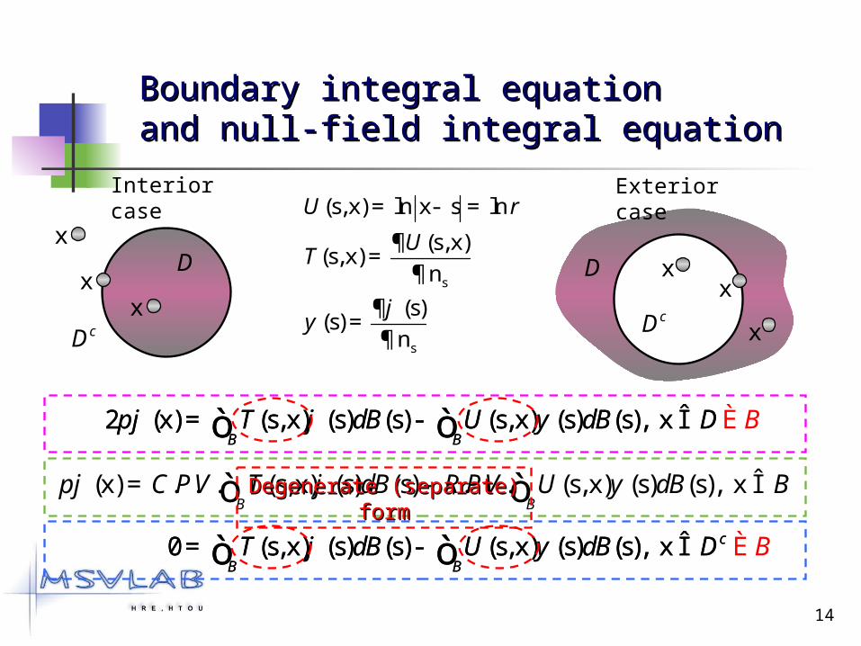
Boundary integral equation Boundary integral equation and null-field integral equationand null-field integral equation

Interior case Exterior case

cD

D D

x

xx

xcD

s

s

(s, x) ln x s ln

(s, x)(s, x)

n

(s)(s)

n

U r

UT

jy

= - =

¶=

¶

¶=

¶

0 (s, x) (s) (s) (s, x) (s) (s), x c

B BT dB U dB Dj y= - Îò ò

(x) . . . (s, x) (s) (s) . . . (s, x) (s) (s), xB B

C PV T dB R PV U dB Bpj j y= - Îò ò

2 (x) (s, x) (s) (s) (s, x) (s) (s), xB BT dB U dB Dpj j y= - Îò ò

x x

2 (x) (s, x) (s) (s) (s, x) (s) (s), xB BT dB U dB D Bpj j y= - Î Èò ò

0 (s, x) (s) (s) (s, x) (s) (s), x c

B BT dB U d D BBj y= - Î Èò ò

Degenerate (separate) formDegenerate (separate) form

15

Outlines (Direct problem)Outlines (Direct problem)




Numerical examplesNumerical examples Degenerate scaleDegenerate scale ConclusionsConclusions

16

Gain of introducing the degenerate Gain of introducing the degenerate kernelkernel

(x) (s, x) (s) (s)BK dBj f=ò

Degenerate kernel Fundamental solution

CPV and HPV

No principal value?

0

(x) (s)(x) (s) (s)jBj

ja dBbj f¥

=

= åò

0

0

(s,x) (s) (x), x s

(s,x)

(s,x) (x) (s), x s

ij j

j

ej j

j

K a b

K

K a b

¥

=

¥

=

ìïï = <ïïïï=íïï = >ïïïïî

å

åinterior

exterior

17

How to separate the regionHow to separate the region

18

Expansions of fundamental solution Expansions of fundamental solution and boundary densityand boundary density

Degenerate kernel - fundamental Degenerate kernel - fundamental solutionsolution

Fourier series expansions - boundary Fourier series expansions - boundary densitydensity

1

1

1( , ; , ) ln ( ) cos ( ),

(s, x)1

( , ; , ) ln ( ) cos ( ),

i m

m

e m

m

U R R m Rm R

UR

U R m Rm

rq r f q f r

q r f r q f rr

¥

=

¥

=

ìïï = - - ³ïïïï=íïï = - - >ïïïïî

å

å

01

01

(s) ( cos sin ), s

(s) ( cos sin ), s

M

n nn

M

n nn

u a a n b n B

t p p n q n B

q q

q q

=

=

= + + Î

= + + Î

å

å

19

Separable form of fundamental Separable form of fundamental solution (1D)solution (1D)

-10 10 20

2

4

6

8

10

Us,x

2

1

2

1

(x) (s), s x

(s, x)

(s) (x), x s

i ii

i ii

a b

U

a b

=

=

ìïï ³ïïïï=íïï >ïïïïî

å

å

1(s x), s x

1 2(s, x)12

(x s), x s2

U r

ìïï - ³ïïï= =íïï - >ïïïî

-10 10 20

-0.4

-0.2

0.2

0.4

Ts,x

s

Separable Separable propertyproperty

continuocontinuousus

discontidiscontinuousnuous

1, s x

2(s, x)1

, x s2

T

ìïï >ïïï=íï -ï >ïïïî

20-20 -15 -10 -5 0 5 10 15 20-20

-15

-10

-5

0

5

10

15

20

Separable form of fundamental Separable form of fundamental solution (2D)solution (2D)

-20 -15 -10 -5 0 5 10 15 20-20

-15

-10

-5

0

5

10

15

20

Ro

s ( , )R q=

x ( , )r f=

iU

eU

r

1

1

1( , ; , ) ln ( ) cos ( ),

(s, x)1

( , ; , ) ln ( ) cos ( ),

i m

m

e m

m

U R R m Rm R

UR

U R m Rm

rq r f q f r

q r f r q f rr

¥

=

¥

=

ìïï = - - ³ïïïï=íïï = - - >ïïïïî

å

å

x ( , )r f=

21

Boundary density discretizationBoundary density discretization

Fourier Fourier seriesseries

Ex . constant Ex . constant elementelement

Present Present methodmethod

Conventional Conventional BEMBEM

22

OutlinesOutlines





23

Adaptive observer systemAdaptive observer system

( , )r f

collocation collocation pointpoint

24

OutlinesOutlines





25

Vector decomposition technique for Vector decomposition technique for potential gradientpotential gradient

zx

z x-

(s, x) 1 (s, x)(s, x) cos( ) cos( )

2

U ULr

pz x z x

r r f¶ ¶

= - + - +¶ ¶

(s, x) 1 (s, x)(s, x) cos( ) cos( )

2

T TM r

pz x z x

r r f¶ ¶

= - + - +¶ ¶

Special case Special case (concentric case) :(concentric case) :

z x=

(s, x)(s, x)

ULr r

¶=

¶(s, x)

(s, x)T

M r r¶

=¶

Non-Non-concentric concentric

case:case:

(x)2 (s, x) (s) (s) (s, x) (s) (s), x

(x)2 (s, x) (s) (s) (s, x) (s) (s), x

B B

B B

uM u dB L t dB D

uM u dB L t dB D

r r

ff

p

p

¶= - Î

¶¶

= - Î¶

ò ò

ò ò

n

t

nt

t

n

True normal True normal directiondirection

26

OutlinesOutlines





27

{ }

0

1

2

N

ì üï ïï ïï ïï ïï ïï ïï ïï ï=í ýï ïï ïï ïï ïï ïï ïï ïï ïî þ

t

t

t t

t

M

Linear algebraic equationLinear algebraic equation

[ ]{ } [ ]{ }U t T u=

[ ]

00 01 0

10 11 1

0 1

N

N

N N NN

é ùê úê úê ú= ê úê úê úê úë û

U U U

U U UU

U U U

L

L

M M O M

L

whwhereere

Column vector of Column vector of Fourier coefficientsFourier coefficients(Nth routing circle)(Nth routing circle)

0B1B

Index of Index of collocation collocation

circlecircle

Index of Index of routing circle routing circle

28

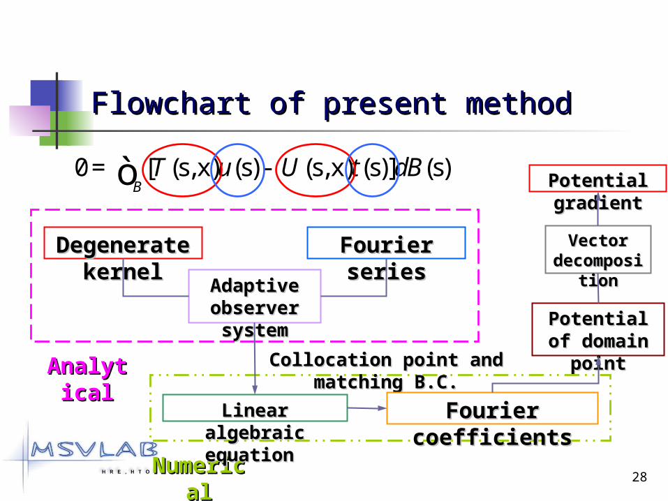
Flowchart of present methodFlowchart of present method

0 [ (s, x) (s) (s, x) (s)] (s)BT u U t dB= -ò

Potential Potential of domain of domain

pointpointAnalytiAnalyticalcal

NumeriNumericalcal

Adaptive Adaptive observer observer systemsystem

DegeneratDegenerate kernele kernel

Fourier Fourier seriesseries

Linear algebraic Linear algebraic equation equation

Collocation point and Collocation point and matching B.C.matching B.C.

Fourier Fourier coefficientscoefficients

Vector Vector decompodecompo

sitionsition

Potential Potential gradientgradient

29

Comparisons of conventional BEM and present Comparisons of conventional BEM and present

methodmethod

BoundaryBoundarydensitydensity

discretizatiodiscretizationn

AuxiliaryAuxiliarysystemsystem

FormulatiFormulationon

ObservObserverer

systemsystem

SingulariSingularityty

ConvergenConvergencece

BoundarBoundaryy

layerlayereffecteffect

ConventionConventionalal

BEMBEM

Constant,Constant,linear,linear,

quadratic…quadratic…elementselements

FundamenFundamentaltal

solutionsolution

BoundaryBoundaryintegralintegralequationequation

FixedFixedobservobserv

erersystemsystem

CPV, RPVCPV, RPVand HPVand HPV LinearLinear AppearAppear

PresentPresentmethodmethod

FourierFourierseriesseries

expansionexpansion

DegeneratDegeneratee

kernelkernel

Null-fieldNull-fieldintegralintegralequationequation

AdaptivAdaptivee

observobserverer

systemsystem

DisappeaDisappearr

ExponentiaExponentiall

EliminatEliminatee

30

OutlinesOutlines





31

Numerical examplesNumerical examples

Laplace equation Laplace equation (EABE 2005, EABE 2007) (EABE 2005, EABE 2007) (CMES 2005, ASME 2007, JoM2007)(CMES 2005, ASME 2007, JoM2007) (MRC 2007, NUMPDE 2010)(MRC 2007, NUMPDE 2010) Biharmonic equation Biharmonic equation (JAM, ASME 2006(JAM, ASME 2006)) Plate eigenproblem Plate eigenproblem (JSV )(JSV ) Membrane eigenproblem Membrane eigenproblem (JCA)(JCA) Exterior acoustics Exterior acoustics (CMAME, SDEE (CMAME, SDEE )) Water waveWater wave (AOR 2009) (AOR 2009)

32

Laplace equationLaplace equation

A circular bar under torqueA circular bar under torque

(free of mesh generation)(free of mesh generation)

33

Torsion bar with circular holes Torsion bar with circular holes removedremoved

The warping The warping functionfunction

Boundary conditionBoundary condition

wherewhere

2 ( ) 0,x x DjÑ = Î

j

sin cosk k k kx yn

jq q

¶= -

¶ kB

2 2cos , sini i

i ix b y b

N N

p p= =

2 k

N

p

a

a

ab q

R

oonn

TorqTorqueue

34

Axial displacement with two circular Axial displacement with two circular holesholes

Present Present method method (M=10)(M=10)

Caulk’s data Caulk’s data (1983)(1983)

ASME Journal of Applied ASME Journal of Applied MechanicsMechanics -2

-1.5

-1

-0.5

0

0.5

1

1.5

2

-2-1.5-1-0.500.511.52

Dashed line: exact Dashed line: exact solutionsolution

Solid line: first-order Solid line: first-order solutionsolution

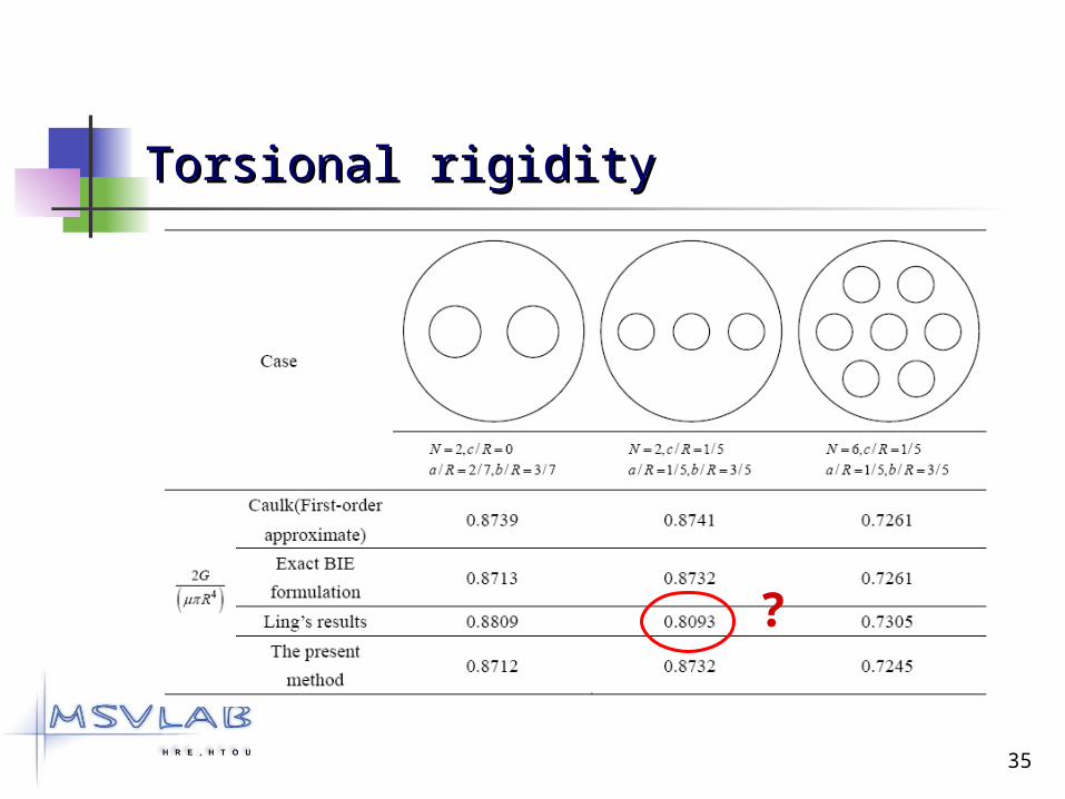
35

Torsional rigidityTorsional rigidity

?

36

Numerical examplesNumerical examples

Biharmonic equationBiharmonic equation (exponential convergence)(exponential convergence)

37

Plate problemsPlate problems

1B

4B

3B

2B1O

4O

3O

2O

Geometric data:

1 20;R 2 5;R

( ) 0u s 1B( ) 0s

1 (0,0),O 2 ( 14,0),O

3 (5,3),O 4 (5,10),O 3 2;R 4 4.R

( ) sinu s

( ) 1u s

( ) 1u s

( ) 0s

( ) 0s

( ) 0s

2B

3B

4B

and

and

and

and

on

on

on

on

Essential boundary conditions:

(Bird & Steele, 1991)

38

Contour plot of displacementContour plot of displacement

-20 -15 -10 -5 0 5 10 15 20-20

-15

-10

-5

0

5

10

15

20

-20 -15 -10 -5 0 5 10 15 20-20

-15

-10

-5

0

5

10

15

20

Present method (N=101)

Bird and Steele (1991)

FEM (ABAQUS)FEM mesh

(No. of nodes=3,462, No. of elements=6,606)

39

Stokes flow problemStokes flow problem

1

2 1R

e

1 0.5R

1B

Governing equation:

4 ( ) 0,u x x

Boundary conditions:

1( )u s u and ( ) 0.5s on 1B

( ) 0u s and ( ) 0s on 2B

2 1( )

e

R R

Eccentricity:

Angular velocity:

1 1

2B

(Stationary)

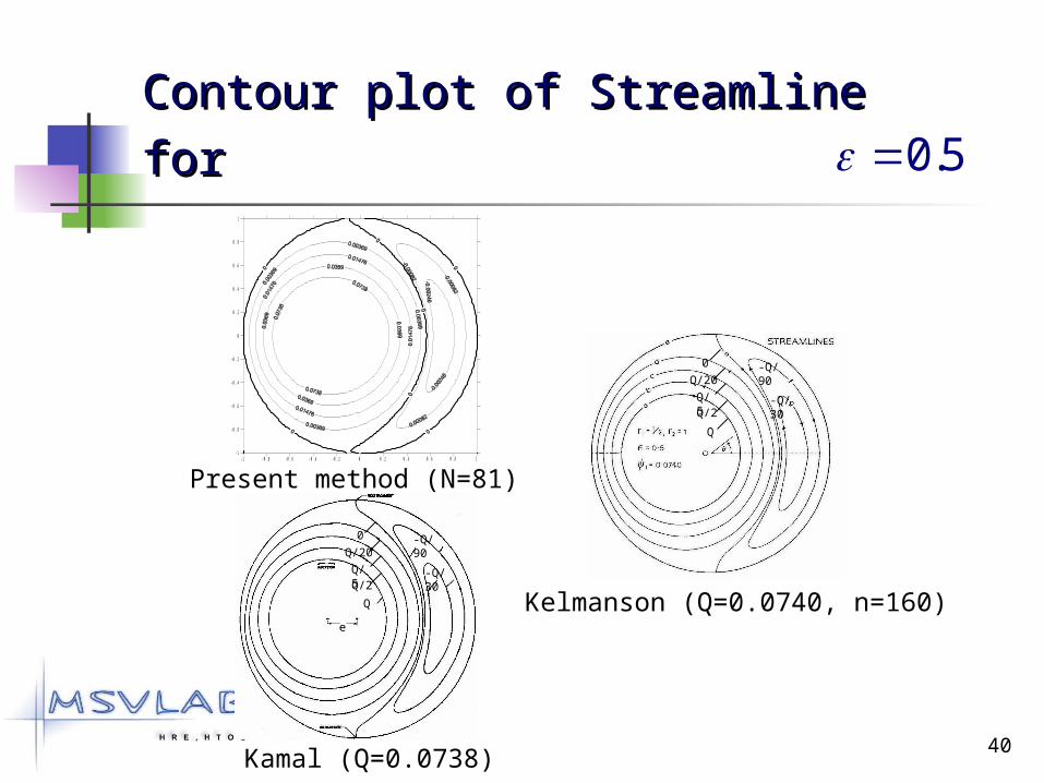
40

Contour plot of Streamline forContour plot of Streamline for

-1 -0.8 -0.6 -0.4 -0.2 0 0.2 0.4 0.6 0.8 1-1

-0.8

-0.6

-0.4

-0.2

0

0.2

0.4

0.6

0.8

1

Present method (N=81)

Kelmanson (Q=0.0740, n=160)

Kamal (Q=0.0738)

e

Q/2

Q

Q/5

Q/20-Q/90

-Q/30

0.5

0

Q/2

Q

Q/5

Q/20-Q/90

-Q/30

0

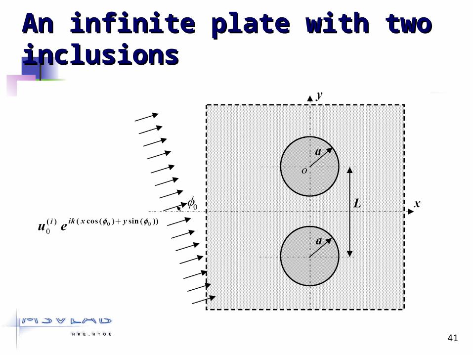
41

An infinite plate with two inclusionsAn infinite plate with two inclusions

42

Distribution of dynamic moment concentration factors Distribution of dynamic moment concentration factors

by using the present method and FEM( by using the present method and FEM( L/a L/a = = 2.12.1))

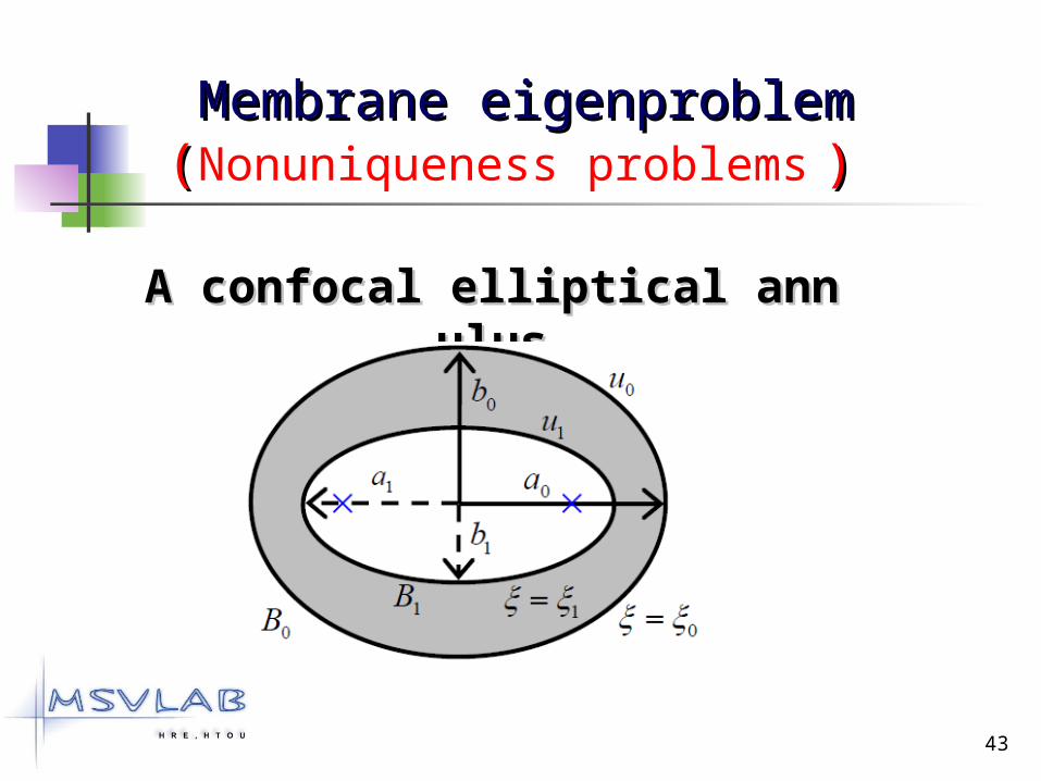
43

Membrane eigenproblemMembrane eigenproblem ((Nonuniqueness problems ))

A confocal elliptical annulusA confocal elliptical annulus

44

A confocal elliptical annulusA confocal elliptical annulus

2 2( ) ( ) 0,k u D x x

0 1( ) 0,u B B x x

G. E.:

B. Cs.:

1

1

1 11

1

2 21 1

0 1

0 0

0 0

1

0.5

tanh

2

cosh( )

sinh( )

a

b

ab

c a b

a c

b c

45

True and spurious eigenvaluesTrue and spurious eigenvalues

Note: the data inside parentheses denote the spurious eigenvalue.

(42)

(11)

Eigenvalues of an elliptical membrane

UT equation Spurious

BEM mesh FEM mesh

True 1

1

( , ) 0

( , ) 0m

m

Je q

Jo q

46

(42)

Mode shapesMode shapes

Even Odd EvenEven Odd

47

Water waveWater wave ((Nonuniqueness problems ))

Interaction of water waves Interaction of water waves with vertical cylinderswith vertical cylinders

48

Trapped modeTrapped mode （（ nonuniqueness in physics nonuniqueness in physics ））

M.S. Longuet-higgins

JFM, 1967.

A.E.H. Love

1966.

Williams & Li

OE, 2000.

49

Trapped and near-trapped modes

Near-trapped mode

Trapped mode

50

Numerical and physical resonanceNumerical and physical resonancePhysical resonance Fictitious frequency

(BEM/BIEM)

t(a,0)

0 2 4 6 8

-2

-1

0

1

2UT method

LM method

Burton & Miller method

1),( au0),( au

Drruk ),( ,0),()( 22

9

1),( au0),( au

Drruk ),( ,0),()( 22

9

Present

e i t

51

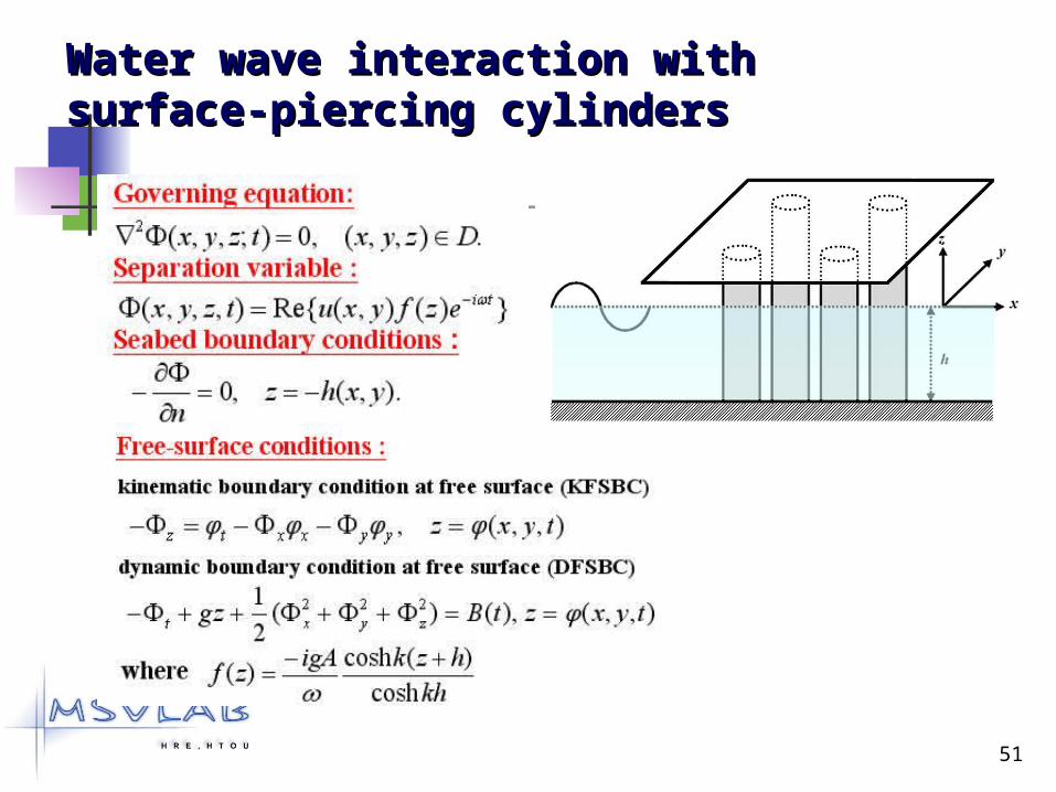
Water wave interaction with surface-piercing Water wave interaction with surface-piercing cylinderscylinders

.),,(,0);,,(2 Dzyxtzyx

( , , , ) Re{ ( , ) ( ) }i tx y z t u x y f z e

Governing equation:

Separation variable :

).,(,0 yxhzn

Seabed boundary conditions :

52

Problem statementProblem statement

2 2( ) ( ) 0,k u x x D

,

.

Dispersion relationship:2

tanhk khg

Dynamic pressure:cosh ( )

( , )cosh

i tk z hp gA u x y e

t kh

Force:2

0

costanh ( , )

sinjjj

jj

gAaX kh u x y d

k

Original problem

inc

Governing equation:

1

2

3

j

53

Sketch of four cylindersSketch of four cylinders

54

Physical phenomenon and fictitious frequencyPhysical phenomenon and fictitious frequency

Near-trapped mode

Fictitious frequency

Near-trapped mode


Near-trapped mode


Near-trapped mode

Near-trapped mode

2.43.8

5.15.5

6.4ka4.08482

55

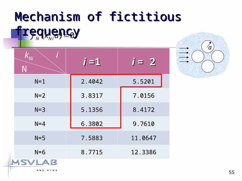
Mechanism of fictitious frequencyMechanism of fictitious frequency

i i =1=1 i i == 2 2

N=1N=1 2.40422.4042 5.52015.5201

N=2N=2 3.83173.8317 7.01567.0156

N=3N=3 5.13565.1356 8.41728.4172

N=4N=4 6.38026.3802 9.76109.7610

N=5N=5 7.58837.5883 11.064711.0647

N=6N=6 8.77158.7715 12.338612.3386

0N N iJ k a a

N

ikNi

56

Near-trapped mode for the four cylinders at Near-trapped mode for the four cylinders at kaka=4.08482 (=4.08482 (a/d=a/d=0.8)0.8)

(a) Contour by the present method (M=20)

57

0 1 2 3 4 5 6 7k a

0

0.5

1

1.5

2

2.5

3C y lin d e r 1

C y lin d e r 2

C y lin d e r 3

E v an s & P o rte r (C y lin d er 1 )



C y lin d e r 1 : 5 4 .0 7 8C y lin d e r 2 : 1 .0 0 0 0C y lin d e r 3 : 5 4 .1 1 1

Near-trapped mode for the four cylinders at Near-trapped mode for the four cylinders at kaka=4.08482 (=4.08482 (aa//dd=0.8)=0.8)

(c) Horizontal force on the four cylinders against wavenumber(b) Free-surface elevations by the present method (M=20)

54

12

34

58

oinc 33

oinc 45

oinc 0 o

inc 15ka=4.08482

59

By perturbing the radius of one cylinder By perturbing the radius of one cylinder (a1/d≠0.8) to destroy the periodical setup(a1/d≠0.8) to destroy the periodical setup

a1/d=0.82

Evans and Porter, JEM ,1999. Present method

0 2 4 6ka

0

1

2

3

4

|X j||F |

a1/d=0.82

C ylinder 1

C ylinder 2 , 4

C ylinder 3

60

Sketch of four cylindersSketch of four cylinders

1 1

61

1 /a d dai /ii=2,3,4=2,3,4

Cylinder 1Cylinder 1 Cylinder 3Cylinder 3

ForceForce ForceForce

0.860.86 0.80.8 1.151.15 0.250.25

0.840.84 0.80.8 1.201.20 0.250.25

0.820.82 0.80.8 1.301.30 0.270.27

0.80.8 0.80.8 54.154.1 54.154.1

0.780.78 0.80.8 1.021.02 0.340.34

0.760.76 0.80.8 1.131.13 0.300.30

0.740.74 0.80.8 1.191.19 0.300.30

'/1 da dai /ii=2,3,4=2,3,4

Cylinder 1Cylinder 1 Cylinder 3Cylinder 3

ForceForce ForceForce

0.860.86 0.80.8 1.151.15 0.290.29

0.840.84 0.80.8 1.201.20 0.280.28

0.820.82 0.80.8 1.271.27 0.270.27

0.80.8 0.80.8 54.154.1 54.154.1

0.780.78 0.80.8 1.121.12 0.270.27

0.760.76 0.80.8 1.171.17 0.260.26

0.740.74 0.80.8 1.161.16 0.260.26

Changing radius Moving the center of one cylinder

ka=4.08482ka=4.08482

Disorder of the periodical patternDisorder of the periodical pattern

62

OutlinesOutlines





63

ConclusionsConclusions

A systematic approach using A systematic approach using degenerate kdegenerate kernelsernels, , Fourier seriesFourier series and and null-field integranull-field integral equationl equation has been successfully proposed has been successfully proposed to solve Laplace Helmholtz and Biharminito solve Laplace Helmholtz and Biharminic problems with circular boundaries.c problems with circular boundaries.

Numerical results Numerical results agree wellagree well with available with available exact solutions, Caulk’s data, Onishi’s dexact solutions, Caulk’s data, Onishi’s data and FEM (ABAQUS) for ata and FEM (ABAQUS) for only few terms only few terms of Fourier seriesof Fourier series..

64


Physical phenomena of Physical phenomena of near-trapped near-trapped mode as well as the numerical instability mode as well as the numerical instability due to due to fictitious frequencyfictitious frequency in BIEM were in BIEM were both observed.both observed.

Fictitious frequency appears and is Fictitious frequency appears and is suppressed in sacrifice of suppressed in sacrifice of higher number higher number of Fourier termsof Fourier terms..

The effect of incident angle and disorder The effect of incident angle and disorder on the near-trapped mode was examined.on the near-trapped mode was examined.

65


Free of boundary-layer effectFree of boundary-layer effect Free of singular integralsFree of singular integrals Well posedWell posed Exponetial convergenceExponetial convergence Mesh-free approachMesh-free approach

66

The EndThe End

Thanks for your kind attentions.Thanks for your kind attentions.Your comments will be highly apprYour comments will be highly appr

eciated.eciated.

URL: URL: http://http://msvlab.hre.ntou.edu.twmsvlab.hre.ntou.edu.tw//

1 null-field integral equations and engineering applications i. l. chen ph.d. department of naval...

Documents

lee slide

principal value slide

literature review motivation

annular plate sh wave

hill green function

canyons degenerate kernel

outlines motivation

nullfield integral equations