1. introduction - tutorialsstaff.civil.uq.edu.au/h.chanson/civ4160/4160_03.pdf · c- a laminar flow...
TRANSCRIPT

CIVL4160 2003/1 Advanced fluid mechanics
CIVL4160-1
1. Introduction - Tutorials
1.1 Physical properties of fluids Give the following fluid and physical properties(at 20 Celsius and standard pressure) with a 4-digit accuracy. Value Units Air density : Water density : Air dynamic viscosity : Water dynamic viscosity : Gravity constant (in Brisbane) :
Surface tension (air and water) :
1.2 Basic equations (1) What is the definition of an ideal fluid ? What is the dynamic viscosity of an ideal fluid ? Can an ideal fluid flow be supersonic ? Explain.
1.3 Basic equations (2) From what fundamental equation does the Navier-Stokes equation derive : a- continuity, b- momentum equation, c- energy equation ? Does the Navier-Stokes equation apply for any type of flow ? If not for what type of flow does it apply for? In a fluid mechanics textbook, find the Navies Stokes equation for a two-dimensional flow in polar coordinates.
1.4 Basic equations (3) For a two-dimensional flow, write the Continuity equation and the Momentum equation for a real fluid in the Cartesian system of coordinates. What is the name of this equation ?
∂ Vx∂x +
∂ Vy∂y = 0
Does the above equation apply to any flow situation ? If not for what type of flow field does the equation apply for ? Write the above equation in a polar system of coordinates. For a two-dimensional ideal fluid flow, write the continuity equation and the Navier-Stokes equation (in the two components) in Cartesian coordinates and in polar coordinates.
CIVL4160 2003/1 Advanced fluid mechanics
CIVL4160-2
1.5 Mathematics If f is a scalar function, and F a vector, verify in a Cartesian system of coordinates that :
curl→
( )grad→
f = 0
div ( ) curl→
F→
= 0
1.6 Flow situations Sketch the streamlines of the following two-dimensional flow situations : A- A laminar flow past a circular cylinder, B- A turbulent flow past a circular cylinder, C- A laminar flow past a flat plate normal to the flow direction, D- A turbulent flow past a flat plate normal to the flow direction. In each case, show the possible extent of the wake (if any). Indicate clearly in which regions the ideal fluid flow assumptions are valid, and in which areas they are not.
Exercise Solutions
1.1 Physical properties of fluids
Solution See Lecture notes, Appendix A.
1.3 & 1.4 Basic equations (2 & 3)
Solution For an incompressible flow the continuity equation is :
div V→
= ∂ Vx∂x +
∂ Vx∂y = 0
The Navier-Stokes equation for a two-dimensional flow is :
ρ
∂ Vx
∂t + Vx * ∂ Vx∂x + Vy *
∂ Vx∂y = -
∂∂x ( )P + ρ *g * z + µ *
∂2 Vx
∂x ∂x + ∂2 Vx∂y ∂y
ρ
∂ Vy
∂t + Vx * ∂ Vy∂x + Vy *
∂ Vy∂y = -
∂∂y ( )P + ρ * g * z + µ *
∂2 Vy
∂x ∂x + ∂2 Vy∂y ∂y
The relationships between Cartesian coordinates and polar coordinates are : x = r * cosθy = r * sinθ
r2 = x2 + y2θ = tan-1
y
x
The velocity components in polar coordinates are deduced from the Cartesian coordinates by a rotation of angle θ : Vx = Vr * cosθ - Vθ * sinθVy = Vr * sinθ + Vθ * cosθ
CIVL4160 2003/1 Advanced fluid mechanics
CIVL4160-3
Vr = Vx * cosθ + Vy * sinθVθ = Vy * cosθ - Vx * sinθ
The continuity and Navier-Stokes equations are transformed using the following formula :
d rdx = cosθ
d rdy = sinθ
d θdx = -
sinθr
d θdy =
cosθr
and dx = dr * cosθ - r * dθ * sinθdy = dr * sinθ + r * dθ * cosθ
dr = dx * cosθ + dy * sinθdθ = 1r * (dy * cosθ - dx * sinθ)
In polar coordinates the continuity equations is :
1r *
∂ (r*Vr)∂r +
1r *
∂ Vθ∂θ = 0
and the Navier-Stokes equation is :
ρ
∂ Vr
∂t + Vr * ∂ Vr∂r +
Vθr *
∂ Vr∂θ -
Vθ2
r =
- ∂∂r ( )P + ρ *g * z + µ *
∆ Vr - Vrr2
- 2r2
* ∂ Vθ∂θ
ρ
∂ Vθ
∂t + Vr * ∂ Vθ
∂r + Vθr *
∂ Vθ∂θ +
Vr * Vθr =
- 1r *
∂∂θ ( )P + ρ *g * z + µ *
∆ Vθ + 2r2
* ∂ Vr∂θ -
Vθr
where :
∆ Vr = 1r *
∂∂r
r * ∂ Vr∂r +
1r2
* ∂2 Vr∂θ2 +
∂2 Vr∂z2
∆ Vθ = 1r *
∂∂r
r * ∂ Vθ
∂r + 1r2
* ∂2 Vθ∂θ2 +
∂2 Vθ∂z2
1.4 Basic equations (3) For a two-dimensional ideal fluid flow, write the continuity equation and the Navier-Stokes equation (in the two components)
Solution For an incompressible flow the continuity equation is :
div V→
= ∂ Vx∂x +
∂ Vy∂y = 0
The Navier-Stokes equation for a two-dimensional flow of ideal fluid is :
ρ
∂ Vx
∂t + Vx * ∂ Vx∂x + Vy *
∂ Vx∂y = -
∂∂x ( )P + ρ *g * z

CIVL4160 2003/1 Advanced fluid mechanics
CIVL4160-4
ρ
∂ Vy
∂t + Vx * ∂ Vy∂x + Vy *
∂ Vy∂y = -
∂∂y ( )P + ρ * g * z
In polar coordinates the continuity equations is :
1r *
∂ (r*Vr)∂r +
1r *
∂ Vθ∂θ = 0
and the Navier-Stokes equation is :
ρ
∂ Vr
∂t + Vr * ∂ Vr∂r +
Vθr *
∂ Vr∂θ -
Vθ2
r = - ∂∂r ( )P + ρ *g * z
ρ
∂ Vθ
∂t + Vr * ∂ Vθ
∂r + Vθr *
∂ Vθ∂θ +
Vr * Vθr = -
1r *
∂∂θ ( )P + ρ *g * z
CIVL4160 2003/1 Advanced fluid mechanics
CIVL4160-5
2. Ideal Fluid Flow - Irrotational Flows - Tutorials
2.1 Quizz - What is the definition of the velocity potential ? - Is the velocity potential a scalar or a vector ? - Units of the velocity potential ? - What is definition of the stream function ? Is it a scalar or a vector ? Units of the stream function ? For an ideal fluid with irrotational flow motion : - Write the condition of irrotationality as a function of the velocity potential. - Does the velocity potential exist for 1- an irrotational flow and 2- for a real fluid ? - Write the continuity equation as a function of the velocity potential. Further, answer the following questions : - What is a stagnation point ? - For a two-dimensional flow, write the stream function conditions. - How are the streamlines at the stagnation point ?
2.2 Basic applications (1) Considering the following velocity field : Vx = y * z * t
Vy = z * x * t
Vz = x * y * t
- Is the flow a possible flow of an incompressible fluid ? - Is the motion irrotational ? If yes : what is the velocity potential ? (2) Draw the streamline pattern of the following stream functions : ψ = 50 * x (1)
ψ = - 20 * y (2)
ψ = - 40 * x - 30 * y (3)
ψ = - 10 * x2 (from x = 0 to x = 5) (4)
2.3 Two-dimensional flow Considering a two-dimensional flow, find the velocity potential and the stream function for a flow having components :
Vx = - 2 * x * y
(x2 + y2)2
Vy = x2 - y2
(x2 + y2)2
CIVL4160 2003/1 Advanced fluid mechanics
CIVL4160-6
2.4 Applications (a) Using the software 2DFlowPlus, investigate the flow field of a vortex (at origin, strength 2) superposed to a sink (at origin, strength 1). Visualise the streamlines, the contour of equal velocity ad the contour of constant pressure. Repeat the same process for a vortex (at origin, strength 2) superposed to a sink (at x=-5, y=0, strength 1). How would you describe the flow region surrounding the vortex. (b) Investigate the superposition of a source (at origin, strength 1) and an uniform velocity field (horizontal direction, V = 1). How many stagnation point do you observe ? What is the pressure at the stagnation point ? What is the "half-Rankine" body thickness at x = +1 ? (You may do the calculations directly or use 2DFlowPlus to solve the flow field.) (c) Using 2DFlowPlus, investigate the flow past a circular building (for an ideal fluid with irrotational flow motion). How many stagnation points is there ? Compare the resulting flow pattern with real-fluid flow pattern behind a circular bluff body (search Reference text in the library). (d) Investigate the seepage flow to a sink (well) located close to a lake. What flow pattern would you use ? Note : the software 2DFlowPlus is described in Appendix D.
2.5 Laplace equation - What is the Laplacian of a function ? Write the Laplacian of the scalar function Φ in Cartesian and polar coordinates. - Rewrite the definition of the Laplacian of a scalar function as a function of vector operators (e.g. grad, div, curl).
2.6 Basic equations (1) For a two-dimensional ideal fluid flow, write : 1- the continuity equation, 2- the streamline equation, 3- the velocity potential and stream function, 4- the condition of irrotationality and 5- the Laplace equation in polar coordinates.
2.7 Basic equations (2) Considering an two-dimensional irrotational flow of ideal fluid :
CIVL4160 2003/1 Advanced fluid mechanics
CIVL4160-7
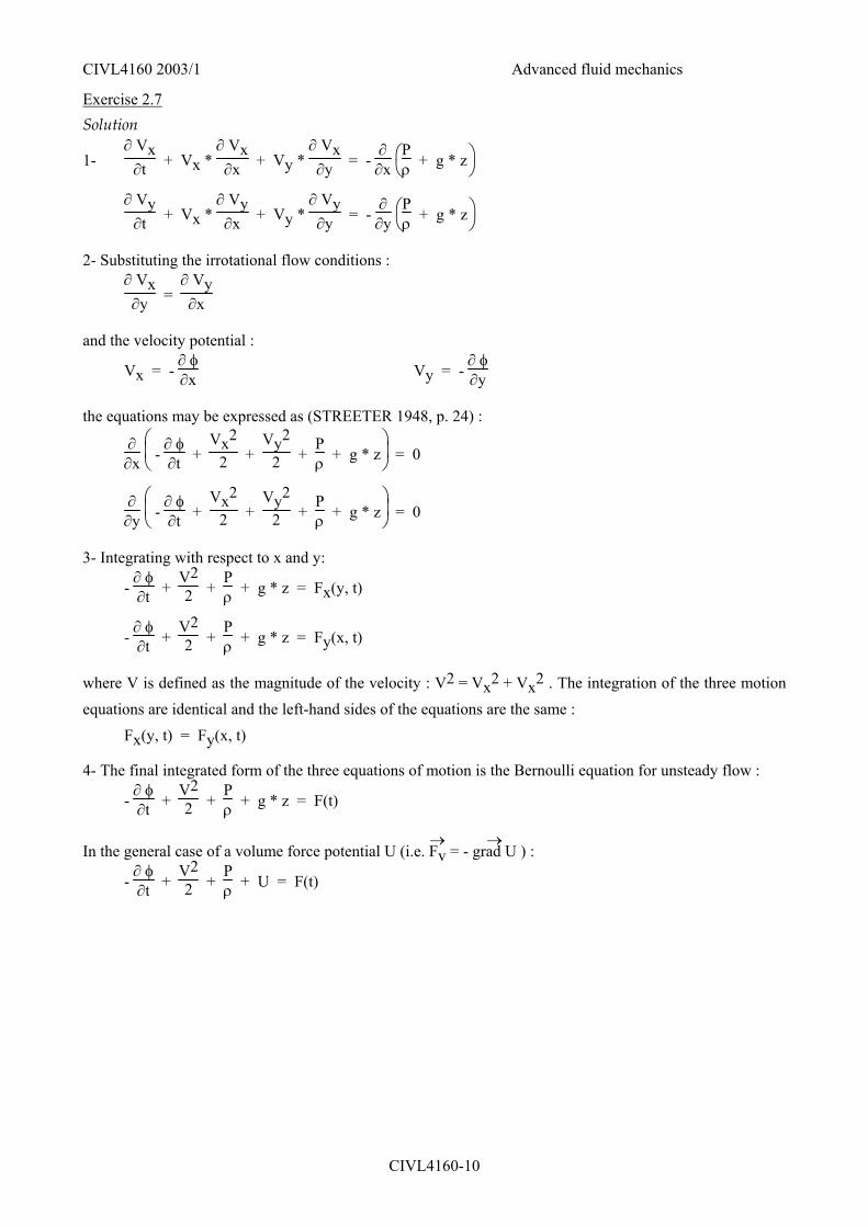
- write the Navier-Stokes equation (assuming gravity forces), - substitute the irrotational flow condition and the velocity potential, - integrate each equation with respect to x and y, - what is the final integrated form of the three equations of motion ? This equation is called the Bernoulli equation for unsteady flow. - For a steady flow write the Bernoulli equation. When the velocity is known, how do you determine the pressure ?
Exercise Solutions
Exercise 2.2
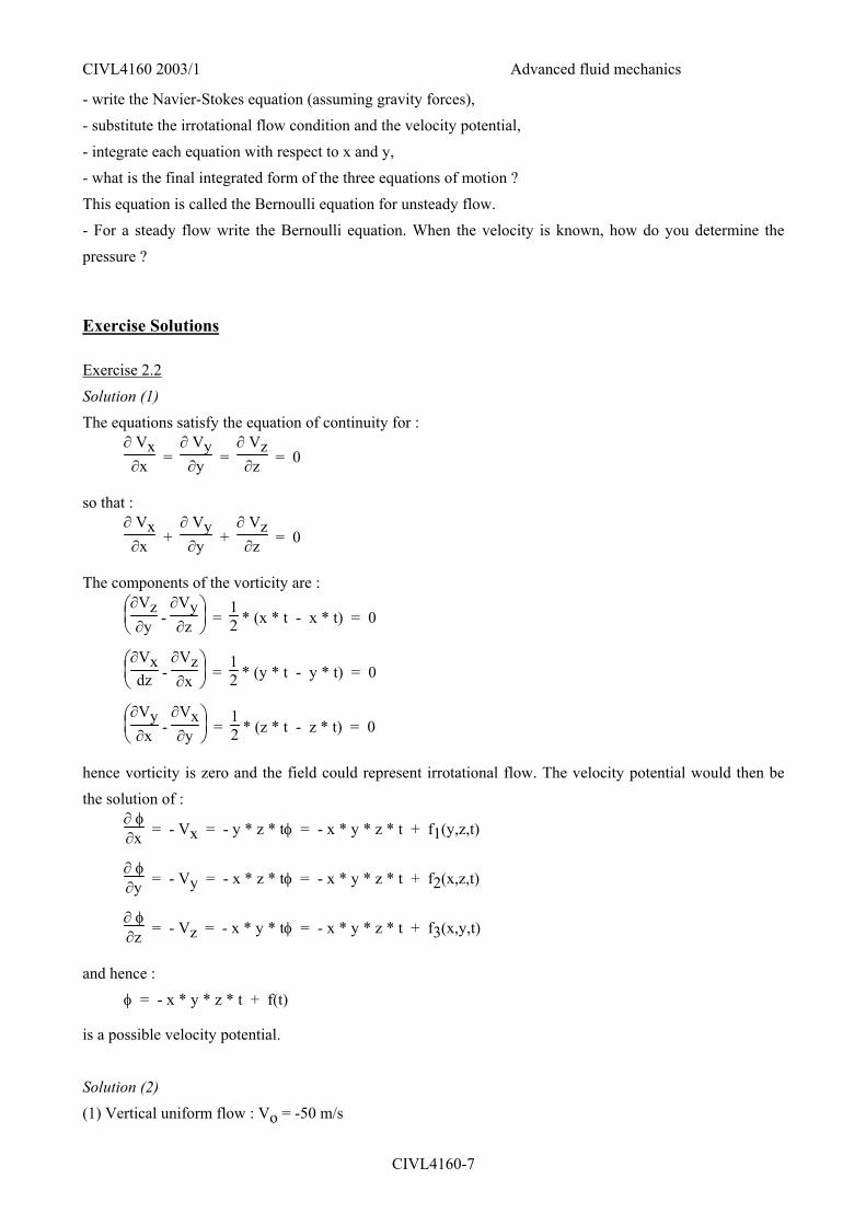
Solution (1) The equations satisfy the equation of continuity for :
∂ Vx∂x =
∂ Vy∂y =
∂ Vz∂z = 0
so that :
∂ Vx∂x +
∂ Vy∂y +
∂ Vz∂z = 0
The components of the vorticity are :
∂Vz
∂y - ∂Vy∂z =
12 * (x * t - x * t) = 0
∂Vx
dz - ∂Vz∂x =
12 * (y * t - y * t) = 0
∂Vy
∂x - ∂Vx∂y =
12 * (z * t - z * t) = 0
hence vorticity is zero and the field could represent irrotational flow. The velocity potential would then be the solution of :
∂ φ∂x = - Vx = - y * z * tφ = - x * y * z * t + f1(y,z,t)
∂ φ∂y = - Vy = - x * z * tφ = - x * y * z * t + f2(x,z,t)
∂ φ∂z = - Vz = - x * y * tφ = - x * y * z * t + f3(x,y,t)
and hence : φ = - x * y * z * t + f(t)
is a possible velocity potential.
Solution (2) (1) Vertical uniform flow : Vo = -50 m/s
CIVL4160 2003/1 Advanced fluid mechanics
CIVL4160-8
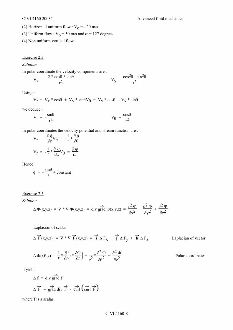
(2) Horizontal uniform flow : Vo = - 20 m/s (3) Uniform flow : Vo = 50 m/s and α = 127 degrees (4) Non uniform vertical flow
Exercise 2.3
Solution In polar coordinate the velocity components are :
Vx = - 2 * cosθ * sinθ
r2 Vy =
cos2θ - sin2θr2
Using : Vr = Vx * cosθ + Vy * sinθVθ = Vy * cosθ - Vx * sinθ
we deduce :
Vr = - sinθr2
Vθ = cosθ
r2
In polar coordinates the velocity potential and stream function are :
Vr = - ∂ φ∂r Vθ = -
1r *
∂ φ∂θ
Vr = - 1r *
∂ ψ∂θ
Vθ = ∂ ψ∂r
Hence :
φ = - sinθ
r + constant
Exercise 2.5
Solution
∆ Φ(x,y,z) = ∇ * ∇ Φ(x,y,z) = div grad→
Φ(x,y,z) = ∂2 Φ∂x2 +
∂2 Φ∂y2 +
∂2 Φ∂z2
Laplacian of scalar
∆ F→
(x,y,z) = ∇ * ∇ F→
(x,y,z) = i→
∆ Fx + j→
∆ Fy + k→
∆ Fz Laplacian of vector
∆ Φ(r,θ,z) = 1r *
∂∂r
r *
∂Φ∂r +
1r2
* ∂2 Φ∂θ2 +
∂2 Φ∂z2 Polar coordinates
It yields :
∆ f = div grad→
f
∆ F→
= grad→
div F→
- curl→
( )curl→
F→
where f is a scalar.
CIVL4160 2003/1 Advanced fluid mechanics
CIVL4160-9
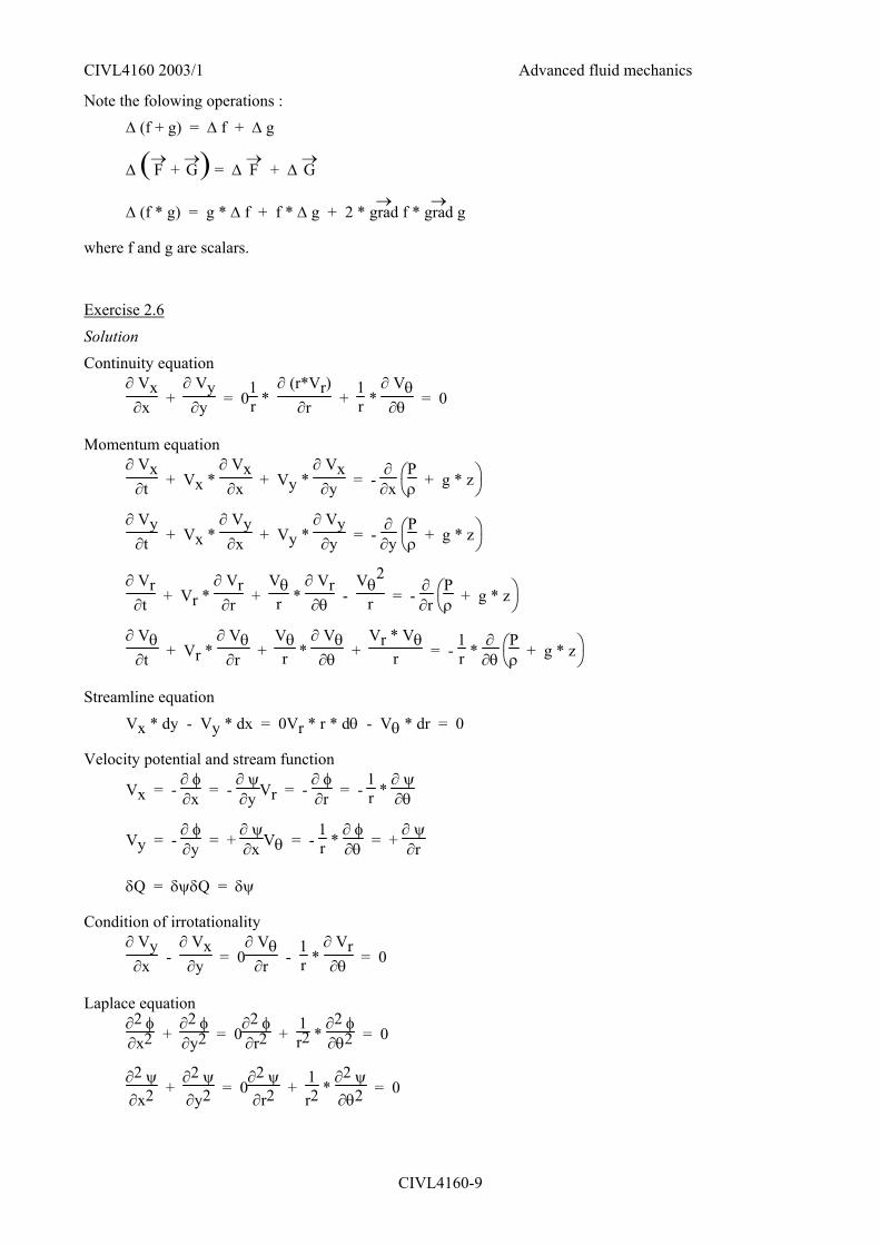
Note the folowing operations : ∆ (f + g) = ∆ f + ∆ g
∆ ( )F→
+ G→
= ∆ F→
+ ∆ G→
∆ (f * g) = g * ∆ f + f * ∆ g + 2 * grad→
f * grad→
g
where f and g are scalars.
Exercise 2.6
Solution Continuity equation
∂ Vx∂x +
∂ Vy∂y = 0
1r *
∂ (r*Vr)∂r +
1r *
∂ Vθ∂θ = 0
Momentum equation
∂ Vx
∂t + Vx * ∂ Vx∂x + Vy *
∂ Vx∂y = -
∂∂x
P
ρ + g * z
∂ Vy
∂t + Vx * ∂ Vy∂x + Vy *
∂ Vy∂y = -
∂∂y
P
ρ + g * z
∂ Vr
∂t + Vr * ∂ Vr∂r +
Vθr *
∂ Vr∂θ -
Vθ2
r = - ∂∂r
P
ρ + g * z
∂ Vθ
∂t + Vr * ∂ Vθ
∂r + Vθr *
∂ Vθ∂θ +
Vr * Vθr = -
1r *
∂∂θ
P
ρ + g * z
Streamline equation Vx * dy - Vy * dx = 0Vr * r * dθ - Vθ * dr = 0
Velocity potential and stream function
Vx = - ∂ φ∂x = -
∂ ψ∂y Vr = -
∂ φ∂r = -
1r *
∂ ψ∂θ
Vy = - ∂ φ∂y = +
∂ ψ∂x Vθ = -
1r *
∂ φ∂θ = +
∂ ψ∂r
δQ = δψδQ = δψ
Condition of irrotationality
∂ Vy∂x -
∂ Vx∂y = 0
∂ Vθ∂r -
1r *
∂ Vr∂θ = 0
Laplace equation
∂2 φ∂x2 +
∂2 φ∂y2 = 0
∂2 φ∂r2 +
1r2 *
∂2 φ∂θ2 = 0
∂2 ψ∂x2 +
∂2 ψ∂y2 = 0
∂2 ψ∂r2
+ 1r2
* ∂2 ψ∂θ2 = 0
CIVL4160 2003/1 Advanced fluid mechanics
CIVL4160-10
Exercise 2.7 Solution
1- ∂ Vx
∂t + Vx * ∂ Vx∂x + Vy *
∂ Vx∂y = -
∂∂x
P
ρ + g * z
∂ Vy
∂t + Vx * ∂ Vy∂x + Vy *
∂ Vy∂y = -
∂∂y
P
ρ + g * z
2- Substituting the irrotational flow conditions :
∂ Vx∂y =
∂ Vy∂x
and the velocity potential :
Vx = - ∂ φ∂x Vy = -
∂ φ∂y
the equations may be expressed as (STREETER 1948, p. 24) :
∂
∂x
- ∂ φ∂t +
Vx2
2 + Vy2
2 + Pρ + g * z = 0
∂
∂y
- ∂ φ∂t +
Vx2
2 + Vy2
2 + Pρ + g * z = 0
3- Integrating with respect to x and y:
- ∂ φ∂t +
V22 +
Pρ + g * z = Fx(y, t)
- ∂ φ∂t +
V22 +
Pρ + g * z = Fy(x, t)
where V is defined as the magnitude of the velocity : V2 = Vx2 + Vx2 . The integration of the three motion equations are identical and the left-hand sides of the equations are the same : Fx(y, t) = Fy(x, t)
4- The final integrated form of the three equations of motion is the Bernoulli equation for unsteady flow :
- ∂ φ∂t +
V22 +
Pρ + g * z = F(t)
In the general case of a volume force potential U (i.e. Fv→
= - grad U→
) :
- ∂ φ∂t +
V22 +
Pρ + U = F(t)
CIVL4160 2003/1 Advanced fluid mechanics
CIVL4160-11
3. Two-Dimensional Flows (1) Basic equations and flow analogies - Tutorials
3.1 Cauchy-Riemann equations - Determine the stream function for parallel flow with a velocity V inclined at an angle α to the x-axis. - Find the velocity potential using the Cauchy-Riemann equations.
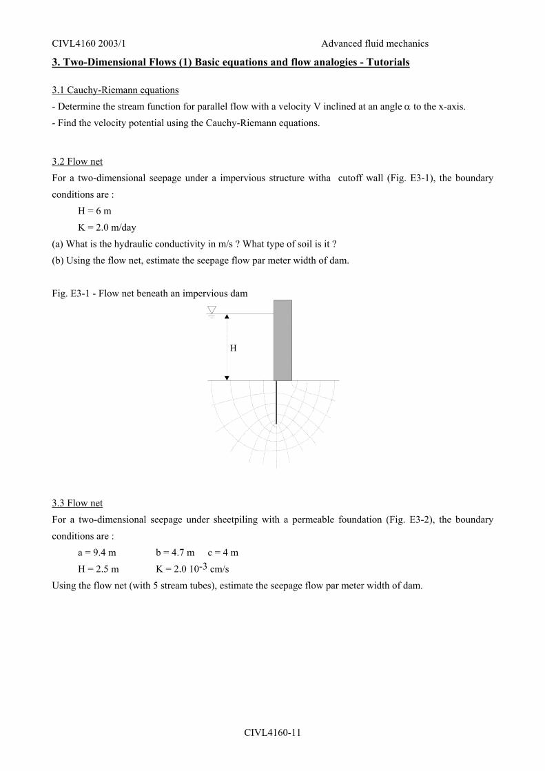
3.2 Flow net For a two-dimensional seepage under a impervious structure witha cutoff wall (Fig. E3-1), the boundary conditions are : H = 6 m K = 2.0 m/day (a) What is the hydraulic conductivity in m/s ? What type of soil is it ? (b) Using the flow net, estimate the seepage flow par meter width of dam. Fig. E3-1 - Flow net beneath an impervious dam
H
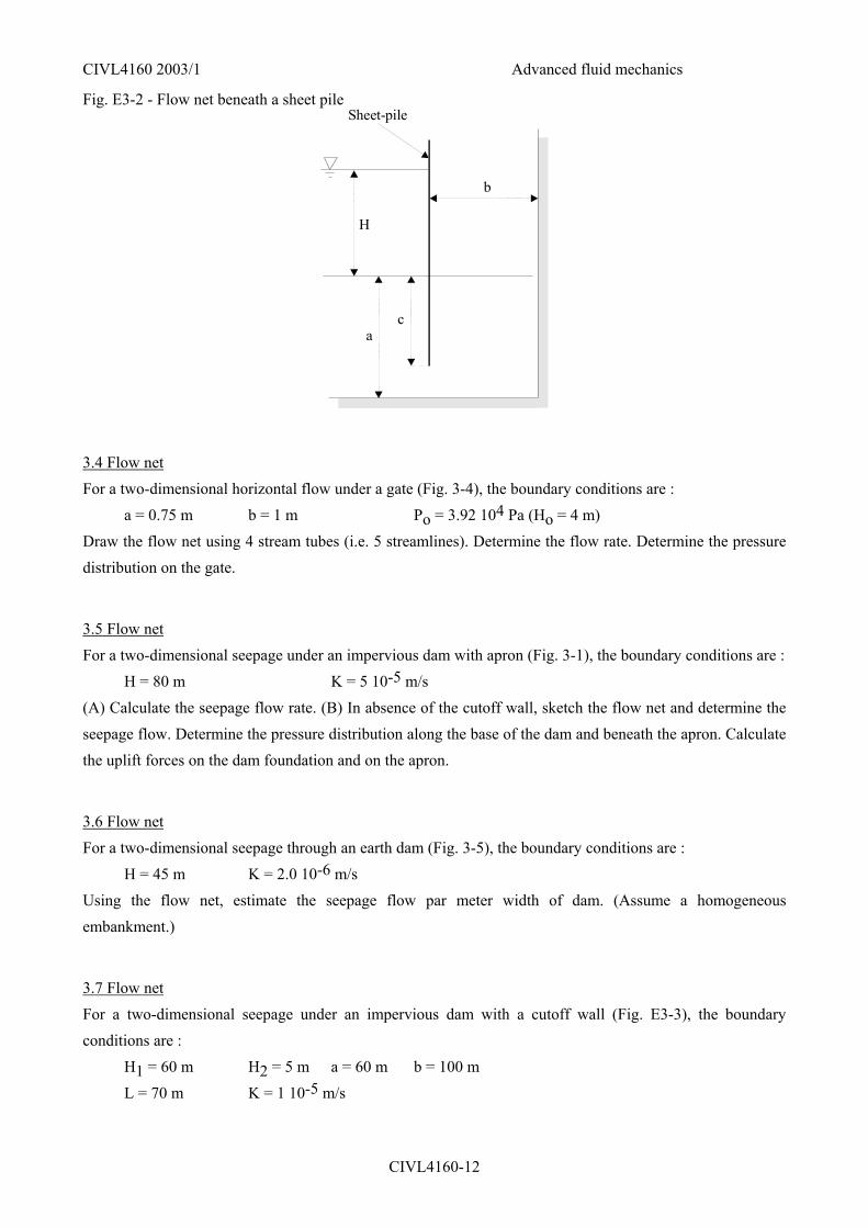
3.3 Flow net For a two-dimensional seepage under sheetpiling with a permeable foundation (Fig. E3-2), the boundary conditions are : a = 9.4 m b = 4.7 m c = 4 m H = 2.5 m K = 2.0 10-3 cm/s Using the flow net (with 5 stream tubes), estimate the seepage flow par meter width of dam.
CIVL4160 2003/1 Advanced fluid mechanics
CIVL4160-12
Fig. E3-2 - Flow net beneath a sheet pile
H
b
Sheet-pile
ac
3.4 Flow net For a two-dimensional horizontal flow under a gate (Fig. 3-4), the boundary conditions are : a = 0.75 m b = 1 m Po = 3.92 104 Pa (Ho = 4 m) Draw the flow net using 4 stream tubes (i.e. 5 streamlines). Determine the flow rate. Determine the pressure distribution on the gate.
3.5 Flow net For a two-dimensional seepage under an impervious dam with apron (Fig. 3-1), the boundary conditions are : H = 80 m K = 5 10-5 m/s (A) Calculate the seepage flow rate. (B) In absence of the cutoff wall, sketch the flow net and determine the seepage flow. Determine the pressure distribution along the base of the dam and beneath the apron. Calculate the uplift forces on the dam foundation and on the apron.
3.6 Flow net For a two-dimensional seepage through an earth dam (Fig. 3-5), the boundary conditions are : H = 45 m K = 2.0 10-6 m/s Using the flow net, estimate the seepage flow par meter width of dam. (Assume a homogeneous embankment.)
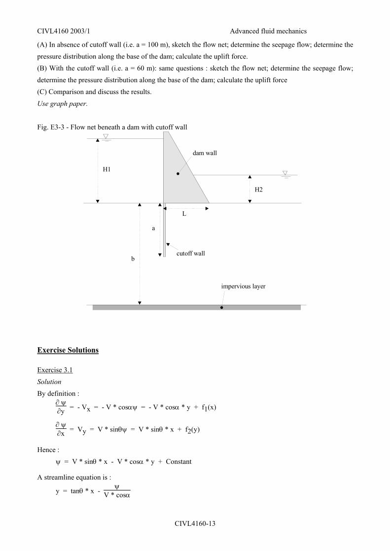
3.7 Flow net For a two-dimensional seepage under an impervious dam with a cutoff wall (Fig. E3-3), the boundary conditions are : H1 = 60 m H2 = 5 m a = 60 m b = 100 m L = 70 m K = 1 10-5 m/s
CIVL4160 2003/1 Advanced fluid mechanics
CIVL4160-13
(A) In absence of cutoff wall (i.e. a = 100 m), sketch the flow net; determine the seepage flow; determine the pressure distribution along the base of the dam; calculate the uplift force. (B) With the cutoff wall (i.e. a = 60 m): same questions : sketch the flow net; determine the seepage flow; determine the pressure distribution along the base of the dam; calculate the uplift force (C) Comparison and discuss the results.
Use graph paper. Fig. E3-3 - Flow net beneath a dam with cutoff wall
H1
H2
a
b
L
dam wall
impervious layer
cutoff wall
Exercise Solutions
Exercise 3.1
Solution By definition :
∂ ψ∂y = - Vx = - V * cosαψ = - V * cosα * y + f1(x)
∂ ψ∂x = Vy = V * sinθψ = V * sinθ * x + f2(y)
Hence : ψ = V * sinθ * x - V * cosα * y + Constant
A streamline equation is :
y = tanθ * x - ψ
V * cosα
CIVL4160 2003/1 Advanced fluid mechanics
CIVL4160-14
which is a straight line equation. The Cauchy-Riemann equations are :
∂ φ∂x =
∂ ψ∂y φ = - V * cosα * x + g1(y)
∂ φ∂y = -
∂ ψ∂x φ = - V * sinθ * y + g2(x)
Hence : φ = - V * sinθ * y - V * cosα * x + Constant
Vx = Vo * cosα Vy = Vo * sinα
ψ = - Vo * (y * cosα - x * sinα)
Exercise 3.2
Solution q = 4.6 m2/day
Exercise 3.3
Solution q = 2.7 m2/day Discussion The flow pattern may be analysed analytically using a finite line source (for the sheet pile) and the theory of images. The resulting streamlines are the equipotentials of the sheet-pile flow. Remember : A velocity potential can be found for each stream function. If the stream function satisfies the Laplace equation the velocity potential also satisfies it. Hence the velocity potential may be considered as stream function for another flow case. The velocity potential φ and the stream function ψ are called "conjugate functions" (Chapter 2, paragraph 4.2).
Exercise 3.4
Solution The problem is similar to Application No. 2, paragraph 2.3. The pressure distribution on the gate is deduced from the Bernoulli principle. Note that the pressure is zero (i.e. atmopsheric) at the orifice edge. While the velocity nor flow rate are given, the flow velocity downstream of the orifice may be deduced from the Bernoulli equation. If the pressure upstream of the gate is much greater than the hydrostatic pressure downstream of the gate, the downstream flow velocity is about : V ~ 2*g*Ho.
Exercise 3.5
Solution
CIVL4160 2003/1 Advanced fluid mechanics
CIVL4160-15
(A) The problem is similar to the flow net sketched in Figure 3-1B (Lecture notes, Chapter 3, paragaph 2.2). (B) In absence of cutoff wall, the streamlines are shorter and the seepage flow rate is greater. The uplift pressure on the dam foundation and apron become very significant. The apron structure would be subjected to high risks of uplift and damage.
Exercise 3.6
Solution See Lecture Notes, Chapter 3, Application, paragraph 3.3.
CIVL4160 2003/1 Advanced fluid mechanics
CIVL4160-16
4. Two-Dimensional Flows (2) Basic flow patterns - Tutorials
4.1 Flow pattern (1) In two-dimensional flow what is the nature of the flow given by : φ = 7 * x + 2 * Ln(r)
Draw the flow net and deduce the main characteristics of the flow field.
4.2 Doublet in uniform flow (1) Select the strength of doublet needed to portray an uniform flow of ideal fluid with a 20 m/s velocity around a cylinder of radius 2 m.
4.3 Flow pattern (2) Considering a vortex (strength +K) and a doublet (strength +µ) at the origin : 1- What are the potential and stream functions ? 2- What are the velocity components in Cartesian and polar coordinates ? 3- Sketch the streamlines and equipotential lines
4.4 Source and sink A source discharging 0.72 m2/s is located at (-1, 0) and a sink of twice the strength is located at (+2, 0). For dynamic pressure at the origin of 7.2 kPa, ρ = 1,240 kg/m3, find the velocity and dynamic pressure at (0, 1) and (1, 1)
4.5 Doublet in uniform flow (2) We consider the air flow (Vo = 9 m/s, standard conditions) past a suspension bridge cable (Ø = 20 mm), (a) Select the strength of doublet needed to portray the uniform flow of ideal fluid around the cylindrical cable. (b) In real fluid flow, calculate the hydrodynamic frequency of the vortex shedding.
4.6 Flow pattern (2) In two-dimensional flow we now consider a source, a sink and an uniform stream. For the pattern resulting from the combinations of a source (located at (-L, 0)) and sink (located at (+L, 0)) of equal strength Q in uniform flow (velocity +Vo parallel to the x-axis) : (a) Sketch streamlines and equipotential lines; (b) Give the velocity potential and the stream function. This flow pattern is called the flow past a Rankine body. W.J.M. RANKINE (1820-1872) was a Scottish engineer and physicist who developed the theory of sources and sinks. The shape of the body may be altered by varying the distance between source and sink (i.e. 2*L) or by varying the strength of the source and sink.
CIVL4160 2003/1 Advanced fluid mechanics
CIVL4160-17
Other shapes may be obtained by the introduction of additional sources and sinks and RANKINE developed ship contours in this way. (c) What is the profile of the Rankine body (i.e. find the streamline that defines the shape of the body)? (d) What is the length and height of the body ? (e) Explain how the flow past a cylinder can be regarded as a Rankine body. Give the radius of the cylinder as a function of the Rankine body parameter.
4.7 Flow pattern (3) In two-dimensional flow we consider again a source, a sink and an uniform stream. But. the source is located at (+L, 0) and the sink is located at (-L, 0) (i.e. opposite to a Rankine body flow pattern). They are of equal strength q in an uniform flow (velocity +Vo parallel to the x-axis). Derive the relationship between the discharge q, the length L and the flow velocity such that no flow injected at the source becomes trapped into the sink.
4.8 Rankine body (1) (a) We consider a Rankine body (Length = 3 m, Breadth = 1.2 m) in an uniform velocity field (horizontal direction, V = 3 m/s) using a source and sink of equal strength. Calculate the source/sink strength and the distance between source and sink. Draw the flow net on a graph paper. (b) Using 2DFlowPlus, investigate the flow pattern resulting by addition of one source (strength +5) at (X=-3,Y=0) and one sink (strength -5) at (X=+3,Y=0) in an uniform flow (V∞ = 1). Plot the pressure and velocity field. Note : the software 2DFlowPlus is presented in Appendix D.
4.9 Source an sink in uniform flow Using the software 2DFlowPlus, investigate the flow pattern resulting by addition of one source (strength +5) at (X=+3,Y=0) and one sink (strength -5) at (X=-3,Y=0) in an uniform flow (V∞= 1). Plot the pressure and velocity field. Where are located the stagnation points ?
4.10 Rankine body (2) (a) Plot the flow net for a Rankine body (Length = 3, Breadth = 1.35) in an uniform velocity field (horizontal direction, V = 3.5) with a source and sink of equal strength. (b) Using 2DFlowPlus, investigate the flow pattern resulting by addition of one vortex (K = -0.1) at (X=+3.5,Y=0) and another (K=+0.1) at {X=+4.5,Y=0). Describe in words the physical nature of the flow.
CIVL4160 2003/1 Advanced fluid mechanics
CIVL4160-18
4.11 Magnus effect (1) Two 15-m high rotors 1.5 m in diameter are used to propel a ship. estimate the total longitudinal force exerted upon the rotors when the relative wind velocity is 25 knots, the angular velocity of the rotors is 220 revolutions per minute and the wind direction is at 60º from the bow of the ship. Perform the calculations for (a) an ideal fluid with irrotational motion and (b) a real fluid.
4.12 Magnus effect (2) (a) For the above rotorship application (4.11), what orientation of the vector of relative wind velocity would yield the greatest propulsion force upon the rotorship ? Calculate the magnitude of this force.
Assume a real fluid flow. The result is trivial for ideal fluid with irrotational flow motion. (b) For the same rotorship application (4.11), determine how nearly into the wind the rotorship could sail. That is, at wind angle would the resultant propulsion force be zero ignoring the wind effect on the ship itself.
Exercise Solutions
Exercise 4.1
Solution The velocity potential of a source located at the origin in an uniform stream is :
φ = - Vo * x - Q
2 * π * Ln(r)
The flow pattern described above is the flow past a half-body. The strength of the source and the flow velocity are : Q = - 12.566 m2/sVo = - 7 m/s
Exercise 4.2
Solution (a) A doublet and uniform flow is analog to the flow past a cylinder of radius :
R = - µVo
where µ is the strength of the doublet. Hence : µ = - Vo * R2 = 80 m3/s
Exercise 4.3
Solution The velocity potential and stream function are :
φ = - K
2 * π * θ + µ * cosθ
r ψ = K
2 * π * Ln(r) - µ * sinθ
r
In Cartesian coordinates :
CIVL4160 2003/1 Advanced fluid mechanics
CIVL4160-19
φ = - K
2 * π * tan-1
y
x + µ * x
x2 + y2ψ = K
4 * p * Ln(x2 + y2) - µ * y
x2 + y2
The velocity components are :
Vr = - µ * cosθ
r2 Vθ = K
2 * π * r - µ * sinθ
r2
In Cartesian coordinates :
Vx =
K2 * π * y + µ * (1 - 2*x2)
x2 + y2 Vy = -
K2 * π * x + 2 * µ * x * y
x2 + y2
A streamline is such as :
φ = - K
2 * π * θ + µ * cosθ
r ψ = K
2 * π * Ln(r) - µ * sinθ
r
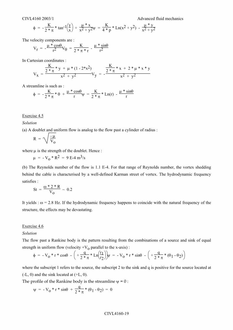
Exercise 4.5
Solution (a) A doublet and uniform flow is analog to the flow past a cylinder of radius :
R = - µVo
where µ is the strength of the doublet. Hence : µ = - Vo * R2 = 9 E-4 m3/s
(b) The Reynolds number of the flow is 1.1 E-4. For that range of Reynolds number, the vortex shedding behind the cable is characterised by a well-defined Karman street of vortex. The hydrodynamic frequency satisfies :
St = ω * 2 * R
Vo ~ 0.2
It yields : ω = 2.8 Hz. If the hydrodynamic frequency happens to coincide with the natural frequency of the structure, the effects may be devastating.
Exercise 4.6
Solution The flow past a Rankine body is the pattern resulting from the combinations of a source and sink of equal strength in uniform flow (velocity +Vo parallel to the x-axis) :
φ = - Vo * r * cosθ -
+
q2 * π * Ln
r1
r2ψ = - Vo * r * sinθ -
+
q2 * π * (θ1 - θ2)
where the subscript 1 refers to the source, the subscript 2 to the sink and q is positive for the source located at (-L, 0) and the sink located at (+L, 0). The profile of the Rankine body is the streamline ψ = 0 :
ψ = - Vo * r * sinθ + q
2 * π * (θ1 - θ2) = 0
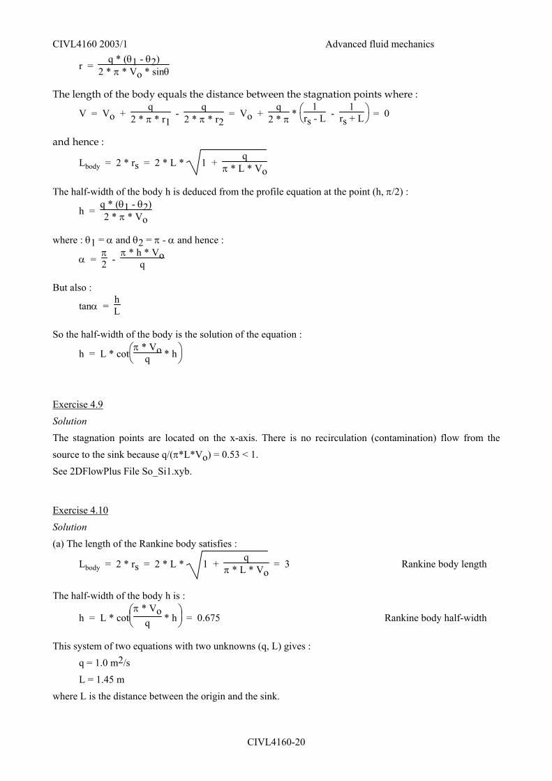
CIVL4160 2003/1 Advanced fluid mechanics
CIVL4160-20
r = q * (θ1 - θ2)
2 * π * Vo * sinθ
The length of the body equals the distance between the stagnation points where :
V = Vo + q
2 * π * r1 -
q2 * π * r2
= Vo + q
2 * π *
1
rs - L - 1
rs + L = 0
and hence :
Lbody = 2 * rs = 2 * L * 1 + q
π * L * Vo
The half-width of the body h is deduced from the profile equation at the point (h, π/2) :
h = q * (θ1 - θ2)2 * π * Vo
where : θ1 = α and θ2 = π - α and hence :
α = π2 -
π * h * Voq
But also :
tanα = hL
So the half-width of the body is the solution of the equation :
h = L * cot
π * Vo
q * h
Exercise 4.9
Solution The stagnation points are located on the x-axis. There is no recirculation (contamination) flow from the source to the sink because q/(π*L*Vo) = 0.53 < 1. See 2DFlowPlus File So_Si1.xyb.
Exercise 4.10
Solution (a) The length of the Rankine body satisfies :
Lbody = 2 * rs = 2 * L * 1 + q
π * L * Vo = 3 Rankine body length
The half-width of the body h is :
h = L * cot
π * Vo
q * h = 0.675 Rankine body half-width
This system of two equations with two unknowns (q, L) gives : q = 1.0 m2/s L = 1.45 m where L is the distance between the origin and the sink.
CIVL4160 2003/1 Advanced fluid mechanics
CIVL4160-21
(b) The addition of vortex is similar to a wake region behind Rankine body.