1 f j i a moving average control chart for the (sample
TRANSCRIPT

1
I !
J 1 f J I A MOVING AVERAGE CONTROL CHART FOR THE (SAMPLE MEAN BASED ON A ROBUST ESTIMATOR J OFSCALE t I &
I t t
by
SUFFIAH BINTI JAMEL
Dissertation submitted in partial fulfillment ·of the requirements for the degree
ofMaster ofScience in Statistics
April2009

ACKNOWLEDGEMENTS
In the name of Allah s.w.t, The Most Gracious and Most Merciful, I would like
to take this opportunity to thank my supervisor, Assosiate Professor Michael Khoo
Boon Chong for his invaluable guidance, advice and supervision throughout my study
and preparation in completing this dissertation. I am certainly unable to complete this
task without his assistance.
I am also indebted to the library of Universiti Sains Malaysia for providing me
with related reference books and journals. Thanks to everyone who has helped me
directly or indirectly throughout my research. Your assistance rendered to me will
always be treasured in my heart.
I would also like to extend my full gratitude to my family, friends and the staffs
of the School of Mathematical Sciences, Universiti Sains Malaysia for their support and
motivation. Thank you very much.
11

CONTENTS
ACKNOWLEDGEMENTS
CONTENTS
LIST OF TABLES
LIST OF FIGURES
ABSTRAK
ABSTRACT
CHAPTER 1: INTRODUCTION
1.1 Quality and Quality Improvement
1.2 A brief Discussion on Statistical Quality Control and Improvement
1.3 Objectives of the Dissertation
1.4 Organization of the Dissertation
CHAPTER 2: CONVENTIONAL CONTROL CHART S
2.1 The X - R Control Charts
2.2 The X - S Control Charts
2.3 The Moving Average (MA) Control Chart
CHAPTER 3: A REVIEW ON SOME ROBUST CONTROL CHARTS
3.1 The Robust X Q - RQ Charts
3.2 The Hodges-Lehmann Control Chart
111
ii
iii
v
vi
vii
viii
1
5
8
9
11
15
18
21
25

3.3
3.4
3.5
A Robust Control Chart based on the Hodges-Lehmann and
Shamos-Bickel-Lehmann Estimators
The x• and s• Charts based on Downton's Estimator
The EWMA Control Chart based on Downton's Estimator
CHAPTER 4: A PROPOSED ROBUST MOVING AVERAGE CONTROL
CHART
4.1 Introduction
4.2 Outliers and their Causes
4.3 A Proposed MAIQR Chart
4.4 Evaluating the Performance of the MAIQR Chart
4.5 An Example of Application
4.6 Discussion
CHAPTER 5: CONCLUSION
5.1
5.2
5.3
5.4
Introduction
Contributions of the Dissertation
Areas for Further Research
Conclusion
REFERENCES
APPENDICES
Appendix A
AppendixB
IV
28
31
36
44
45
48
49
57
61
62
62
63
64
65
67
68
LIST OF TABLES
Pages
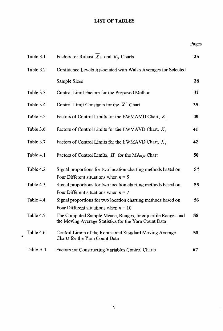
Table 3.1 Factors for Robust X Q and RQ Charts 25
Table 3.2 Confidence Levels Associated with Walsh Averages for Selected
Sample Sizes 28
Table 3.3 Control Limit Factors for the Proposed Method 32
Table 3.4 Control Limit Constants for the x• Chart 35
Table 3.5 Factors of Control Limits for the EWMAMD Chart, K 1 40
Table 3.6 Factors ofControl Limits for the EWMAVD Chart, K 2 41
Table 3.7 Factors of Control Limits for the EWMA VD Chart, K 3 42
Table 4.1 Factors of Control Limits, H 1 for the MA1QR Chart 50
Table 4.2 Signal proportions for two location charting methods based on 54
Four Different situations when n = 5
Table 4.3 Signal proportions for two location charting methods based on 55
Four Different situations when n = 7
Table 4.4 Signal proportions for two location charting methods based on 56
Four Different situations when n = 10
Table 4.5 The Computed Sample Means, Ranges, Interquartile Ranges and 58 the Moving Average Statistics for the Yam Count Data
Table 4.6 Control Limits of the Robust and Standard Moving Average 58 • Charts for the Yam Count Data
Table A.1 Factors for Constructing Variables Control Charts 67
v
LIST OF FIGURES
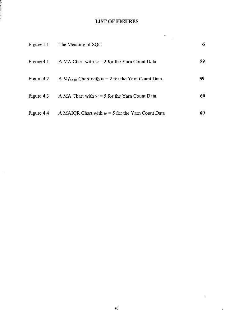
Figure 1.1 The Meaning of SQC 6
Figure 4.1 A MA Chart with w = 2 for the Yam Count Data 59
Figure 4.2 A MArQR Chart with w = 2 for the Yam Count Data 59
Figure 4.3 A MA Chart with w = 5 for the Yam Count Data 60
Figure 4.4 A MAIQR Chart with w = 5 for the Yam Count Data 60
VI
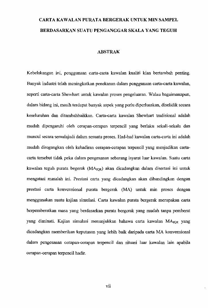
CARTA KA WALAN PURA TA BERGERAK UNTUK MIN SAMPEL
BERDASARKANSUATUPENGANGGARSKALAYANGTEGUH
ABSTRAK
Kebelakangan ini, penggunaan carta-carta kawalan kualiti kian bertambah penting.
Banyak industri telah meningkatkan penekanan dalam penggunaan carta-carta kawalan,
seperti carta-carta Shewhart untuk kawalan proses pengeluaran. Walau bagaimanapun,
dalam bidang ini, masih terdapat banyak aspek yang perlu diperluaskan, diselidik secara
keseluruhan dan ditambahbaikkan. Carta-carta kawalan Shewhart tradisional adalah
mudah dipengaruhi oleh cerapan-cerapan terpencil yang berlaku sekali-sekala dan
muncul secara semulajadi dalam sesuatu proses. Had-had kawalan carta-carta ini adalah
mudah diregangkan oleh kehadiran cerapan-cerapan terpencil yang menjadikan carta
carta tersebut tidak peka dalam pengesanan sebarang isyarat luar kawalan. Suatu carta
kawalan teguh purata begerak (MArQR) akan dicadangkan dalam disertasi ini untuk
mengatasi masalah ini. Prestasi carta yang dicadangkan akan dibandingkan dengan
prestasi carta konvensional purata bergerak (MA) untuk min proses dengan
menggunakan suatu kajian simulasi. Carta kawalan purata bergerak merupakan carta
berpemberatkan masa yang berdasarkan purata bergerak yang mudah tanpa pemberat
yang diminati. Kajian simulasi menunjukkan bahawa carta kawalan MArQR yang
dicadangkan memberikan keputusan yang lebih baik daripada carta MA konvensional
dalam pengesanan cerapan-cerapan terpencil dan situasi luar kawalan lain apabila
cerapan-cerapan terpencil hadir.
Vll
ABSTRACT
Lately, the use of quality control charts is becoming more important. Many industries
have given increased emphasis on using control charts, such as the Shewhart charts in
the monitoring of manufacturing processes. In this area, however, there are still many
aspects that need to be extended, generalized and improved upon. The traditional
Shewhart control charts are easily affected by occasional outliers that might be a natural
part of a process. The limits of these charts are easily stretched by the presence of
outliers, making them insensitive in the detection of any out-of-control signal. A robust
moving average (MA1oR) chart will be proposed in this dissertation to overcome this
problem. The performance of the proposed chart is compared with that of the
conventional moving average (MA) chart for the process mean using a simulation
study. A moving average control chart is a time weighted chart based on a simple,
unweighted moving average of interest, where the chart's statistics incorporates past
sample points. The simulation study shows that the proposed MAIQR control chart
provides superior results to that of the conventional MA chart in the detection of
outliers and other forms of out-of-control situations when outliers are present.
Vlll
CHAPTER!
INTRODUCTION
1.1 Quality and Quality Improvement
Quality can be defined in many ways, rangmg from "satisfying customers'
requirements" to "fitness for use" and "conformance to requirement". It is obvious that
any definition of quality should include customer satisfaction which is the primary goal
of any business. In almost all cases, most people have a conceptual understanding of
quality as relating to one or more desirable characteristics that a product or service
should possess (Montgomery, 2005).
Quality is the overall features and characteristics of a product or service that bear on its
ability to satisfy given needs. This definition is the consensus definition in the
ANSI/ASQC Standard A3 (1978), a document that provides a comprehensive discussion
of quality and related terms. Quality can affect other vital elements of a company such
as productivity, cost, delivery schedules, and skills and expertise of the employees
including management. It may also have an effect on the workplace environment.
Quality also leaves its imprint on society in terms of health, education, cultural and
moral values (Montgomery, 2005).
One of the most important consumer decision factors in the selection among competing
products and services is quality. The phenomenon is widespread, regardless of whether
the -consumer is an individual, an industrial organization, a retail store or a military
1
defense program. As -a result, the key factor leading to business success, growth and an
enhanced competitive position is to understand and improve the quality of a product.
Garvin (1987) provides an excellent discussion of eight components or dimensions of
quality in order to differentiate the quality of a product. In accordance with Garvin, the
components of quality can be summarized as follow:
(i) Performance
Customers usually evaluate the ability of a product to function properly. For
example, customers evaluate spreadsheet software packages for a PC to
determine the data manipulation operations they perform. Customers will be
more agreeable with a particular product if it outperforms the other competing
products.
(ii) Reliability
The reliability of an item is the probability that it will adequately perform its
specified purpose for a specified period of time under specified environmental
conditions. For example, an automobile will requires occasional repairs, but if it
requires frequent repairs, then it is unreliable.
(iii) Durability
This component indicates the effective service life of a product which is very
important to most customers. Customers always want products that perform
satisfactorily over a long period of time.
2
(iv) Serviceability
A customer's view of quality is directly influenced by how quickly and
economically a repair or routine maintenance activity can be accomplished.
Examples include the appliance and automobile industries and the various types
of service industries.
(v) Aesthetics
The outlook of a product such us style, colour, shape, packaging alternatives,
tactile characteristics, and other sensory features are important in order to
differentiate a product with its competitors.
(vi) Features
Customers always have high expectations with the function of a product, that is,
those that have additional features beyond the basic performance of the product.
For example, a spreadsheet software package is said to have superior quality if it
has built-in statistical analysis features while its competitors do not.
(vii) Perceived Quality
Usually, customers rely on the past reputation of a company concerning the
quality of its products. For example, if customers make regular business trips
using a particular airline, where the flights almost always arrive on time and that
the airline company does not lose or damage any luggage, such customers will
probably prefer to fly on the same airlines.
3
(viii) Conformance to Standards
A high-quality product always meets a customer's requirement. For example,
how well does a hood fits on a new car is a measure of conformance to
standards.
Many of today's problem solving and quality tools such as control charts, acceptance
sampling, process capability analysis and value analysis (VA) were first used
extensively in World War II in response to the needs for tremendous volumes of high
quality and lower cost materials. More recently, Quality Circles, TQM, and Kaizen have
demonstrated the power of team-based process improvement. Process capability and
design of experiments (DOE) have come to the fore in Six Sigma (Brecker, 2001).
Quality control should be considered to be more than a set of principles and techniques.
It is concerned with using the principles and techniques to achieve the benefits of
improved quality, reduced costs, less waste, greater productivity, better deliveries, better
marketability and customer acceptance. When a proper attitude and desire have been
developed and communicated throughout the enterprise, and quality planning is being
carried out, consideration of the latter two categories (quality improvement and quality
control) at the process level will assist implementation and achieve positive results.
Quality improvement and quality control are two aspects of quality that are closely
related. There is no general rule concerning which should be applied or emphasized first.
It varies with the process, product, or service. Applying the procedures to achieve
4
control of quality may reveal places where improvements of quality are needed. On the
other hand, application of techniques to improve quality will often indicate where
procedures of control are necessary and beneficial.
1.2 A Brief Discussion on Statistical Quality Control and Improvement
Statistical quality control is defined as the application of statistical methods to measure
and analyze the output of a process. Statistical quality control, SQC is the use of
statistical techniques to control or improve the quality of the output of some production
and service processes. Figure 1.1 illustrates the meaning of SQC.
Statistical techniques provide the facts that indicate how a process has performed in the
past, how it is performing currently, and make predictions on its future performance.
Thus, SQC provides the basis for actions required in improving process performance
and satisfying customer needs (Garrity, 1993).
The use ofSQC can be summarized as follow (Garrity, 1993):
a) Reduce and eliminate errors, scrap and rework in the process.
b) Improve communication throughout the entire organization.
c) Encourage active participation in quality improvement.
d) Increase involvement in the decision-making process.
e) Simplify and improve work procedures.
f) Manage the process by facts and not opinion.
5

Use of Statis1cal Techniques
Analyze a Prors or its Output
Achieve a State of Statistical Control
Improve Prjess Capability
Figure 1.1 The Meaning ofSQC
Statistical quality control, SQC for repetitive, high volume production began in the
1930's when Shewhart developed control charts. Small production samples were
measured periodically to monitor quality. The sample mean (X) and sample range (R)
charts are used to detect out-of-control points in a process.
The causes ofvariations which make a sample point to plot beyond the upper and lower
control limits must be eliminated in order to bring a process back into statistical control.
Most of the statistical quality control techniques used now have been developed during
the last century. One of the most commonly used statistical tools, i.e., a control chart
was introduced by Dr. Walter Shewhart in 1924 at the Bell Laboratories. The acceptance
sampling techniques were developed by Dr. H. F. Dodge and H. G. Romig in 1928, also
at the Bell Laboratories. Design of experiments, developed by Dr. R. A. Fisher in U.K.
6
is used since in the 1930s. The end of World War II saw an increased interest in quality,
primarily among the industries in Japan. This was mainly due to the efforts of Dr. W. E.
Deming. Since the beginning of 1980s, U.S. industries have strived to improve the
quality of their products. They have been assisted in this endeavour by Dr. Genichi
Taguchi, Philip Crosby, Dr. Deming, and Dr. Joseph M. Juran. Industries in the 1980s
also benefited from the contributions of Dr. Taguchi on designs of experiments, loss
functions, and robust designs. The recent emphasis on teamwork in design has resulted
in concurrent engineering. The standards for a quality system, ISO 9000, were later
modified and enhanced substantially by the U.S. automobile industries, resulting in QS-
9000 (Montgomery, 2005).
The seven major SQC problem solving tools, known as the "Magnificent Seven" are as
follow (Montgomery, 2005):
I. Flow chart: The whole process is diagrammed from start to finish with each step of
the process clearly indicated. Everyone involved in the process should know their
positions on the flow chart and at least a partial upstream and downstream trace from
their positions.
2. Pareto chart: The numbers of occurrences of specific problems are charted on a bar
graph. The longer bars indicate the major problems. A Pareto chart is used to determine
the priorities in problem solving.
3. Check sheet: A data-gathering sheet that categorizes problems or defects. The
information of a check sheet may be put on a Pareto chart or, if a time analysis is
included, may be used to investigate problem trends over time.
7
4. Cause-and-effect diagram: A problem (the effect) is systematically tracked back to
possible causes of the problem. The diagram organizes the search for the root cause of
the problem.
5. Histogram: A bar graph shows the comparative frequency of specific measurements.
The shape of the histogram can indicate that a problem exists at a specific point in a
process.
6. Control chart: A broken-line graph that illustrates how a process or a point in a
process behaves over time. Samples are periodically taken, checked, or measured, and
the results plotted on the chart. The charts can show how the specific measurement
changes, how the variation in a measurement changes, or how the proportion of
defective pieces changes over time.
7. Scatter plot: Pairs of measurements are plotted on a two-dimensional coordinate
system to determine if a relationship exists between the measurements.
1.3 Objectives of the Dissertation
The objectives of the dissertation are to identify the shortcomings ofthe moving average
control chart for the mean when outliers are present and to propose a robust moving
average control chart based on the sample interquartile range (IQR) estimator to
overcome the shortcomings of the standard moving average control chart when outliers
are present.
8

1.4 Organization of the Dissertation
This section discusses the organization of the dissertation. Chapter 1 gives the definition
of quality and quality improvement, and a brief discussion on statistical quality control
and improvement. We also discuss the objectives of this dissertation in this chapter.
Chapter 2 explains the conventional control charts such as the X - R, X - S and moving
average (MA) control charts which are among the most important and useful on-line
statistical quality control techniques.
Some existing robust control charts will be reviewed in Chapter 3. The purpose of this
chapter is to present the existing methods or techniques that solve the problems faced by
conventional control charts when outliers are present.
Chapter 4 is the most important part of this dissertation. It discusses the proposed robust
moving average control chart. The proposed MA1QR chart is applicable for any sample
size. The statistics that are used in the construction of the proposed chart will also be
given. The simulation results, in terms of the proportions of signaling an out-of-control
signal under different situations are also given and compared with that of the standard
moving average chart. Besides, the definition of outliers will also be given in this
chapter.
9
Chapter 5 concludes the research conducted in this dissertation. The contributions ofthe
dissertation will be highlighted. Topics for further research will also be identified in this
chapter.
10.
CHAPTER2
CONVENTIONAL VARIABLES CONTROL CHARTS
2.1 The X- R Control Charts
Assume that a quality characteristic is normally distributed with a known mean J..l and
standard deviation cr. If Xp X 2, ... , Xn is a sample of size n, then the average of this
sample is
X= XI +X2 + ... +Xn
n (2.1)
and we know that X is normally distributed with mean J..l and standard deviation
cr x = Fn . The probability that a sample mean falls between the limits of the X chart,
I.e.,
(2.2a)
and
(2.2b)
is 1 - a (Montgomery, 2005).
Therefore, if the mean J..l and standard deviation cr are known, Equations (2.2a) and
(2.2b) could be used as the upper control limit (UCL) and lower control limit (LCL),
respectively. It is customary to replace Z a 12 by 3, so that the three-sigma limits are
employed. If a sample mean falls outside of these limits, it is an indication that the
11
process mean is no longer equal to Jl· Here, we assume that the distribution of the
quality characteristic is normal. However, the above results are still approximately
correct even if the underlying distribution is slightly nonnormal because of the central
limit theorem.
In practice, usually both J..l and cr are unknown. Therefore, we must estimate these
parameters from a preliminary data set or subgroups taken when the process is thought
to be in-control. These estimates are usually based on at least 20 to 25 samples.
Suppose that m samples are available, each containing n observations on the quality
characteristic. The sample size, n is usually small having a value of 4, 5 or 6. The
sample size is small so that we can reduce the cost of sampling and inspection
(Montgomery, 2005).
Let X 1, X 2 , ... ,X m be the sample mean for each of the m samples, then the best estimator
of Jl is
X= xl +2 X + ... +Xm. m
Here, X is used as the center line (CL) of the control chart.
(2.3)
Let xl'x2, ... , xn be a sample of size n, then the range ofthe sample is the difference
between the largest and the smallest observations, i.e.,
R=X -X. max nun (2.4)
12
Let R = RI + R2 + ... + Rm m
be the average range of these m sample ranges.
An estimator of u can be obtained as
(2.5)
(2.6)
where the value d2 depends on the sample size, n. Values of d2 for the various sample
sizes are given in Table A.l in Appendix A.
If X is an estimator of ll and !!.._ is an estimator of u, then the limits for the X chart d2
are
= 3 -UCL-=X+--R
X d2--/n
CL- =X X
= 3 -LCL-=X---R
X d2-f;;
IfA2 = 31 , then Equations (2.7a), (2.7b) and (2.7c) can be written as
d2 vn
CL- =X X
13
(2.7a)
(2.7b)
(2.7c)
(2.8a)
(2.8b)
(2.8c)
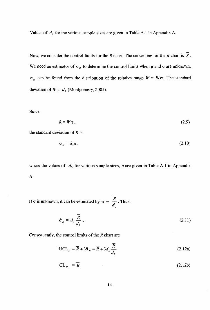
Values of A2 for the various sample sizes are given in Table A.l in Appendix A.
Now, we consider the control limits for the R chart. The center line for the R chart is R.
We need an estimator of a R to determine the control limits when Jl and a are unknown.
a R can be found from the distribution of the relative range W = Rl cr . The standard
deviation of W is d 3 (Montgomery, 2005).
Since,
R = Wcr, (2.9)
the standard deviation of R is
(2.10)
where the values of d3 for various sample sizes, n are given in Table A.l in Appendix
A.
R If a is unknown, it can be estimated by cr = - . Thus,
d2
R crR = d-3d
2
Consequently, the control limits of the R chart are
CLR = R
14
(2.11)
(2.12a)
(2.12b)

•
(2.12c)
Equations (2.12a), (2.12b) and (2.12c) can be written as
UCLR = D4 R (2.13a)
CL = R R (2.13b)
LCLR = D3 R (2.13c)
The values of D3 and D4 for various sample sizes, n are given in Table A.l in
Appendix A. The R chart is plotted first to determine if the process variance is stable
before the X chart is plotted.
2.2 The X - S Control Charts
The S control chart uses the sample standard deviation, S , to monitor changes in the
process variance. Banks (1989) recommended the use of the S control chart instead of
the R chart to monitor process dispersion for larger sample sizes (n > 1 0) and when
sample ·sizes, n are unequal. The sample mean, X and sample standard deviation, S are
used in the construction of the X - S charts. If cr2 is unknown, then an unbiased
estimator of cr 2 is the sample variance
15
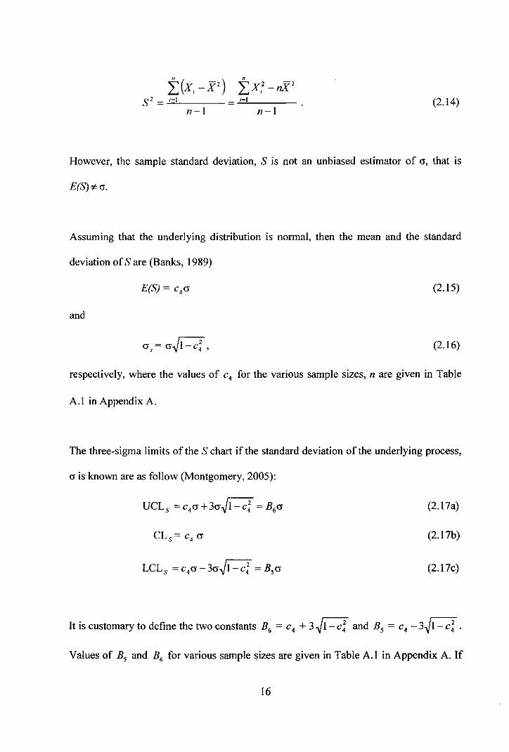
sz = -'-i=...:._l ____ = ....:...i=....:...l ----
n-1 n-1 (2.14)
However, the sample standard deviation, S is not an unbiased estimator of <J, that is
Assuming that the underlying distribution is normal, then the mean and the standard
deviation of S are (Banks, 1989)
(2.15)
and
(J=(J~ s V1 -c;4' (2.16)
respectively, where the values of c4 for the various sample sizes, n are given in Table
A.l in Appendix A.
The three-sigma limits of the S chart if the standard deviation of the underlying process,
<J is known are as follow (Montgomery, 2005):
UCLs = c4cr +3cr~1-ci = B6 cr (2.17a)
(2.17b)
(2.17c)
Itiscustomarytodefinethetwoconstants B6 = c4 +3~1-c; and B5 = c4 -3~1-c;.
Values of B5 and B6 for various sample ~izes are given in Table A.l in Appendix A. If
16
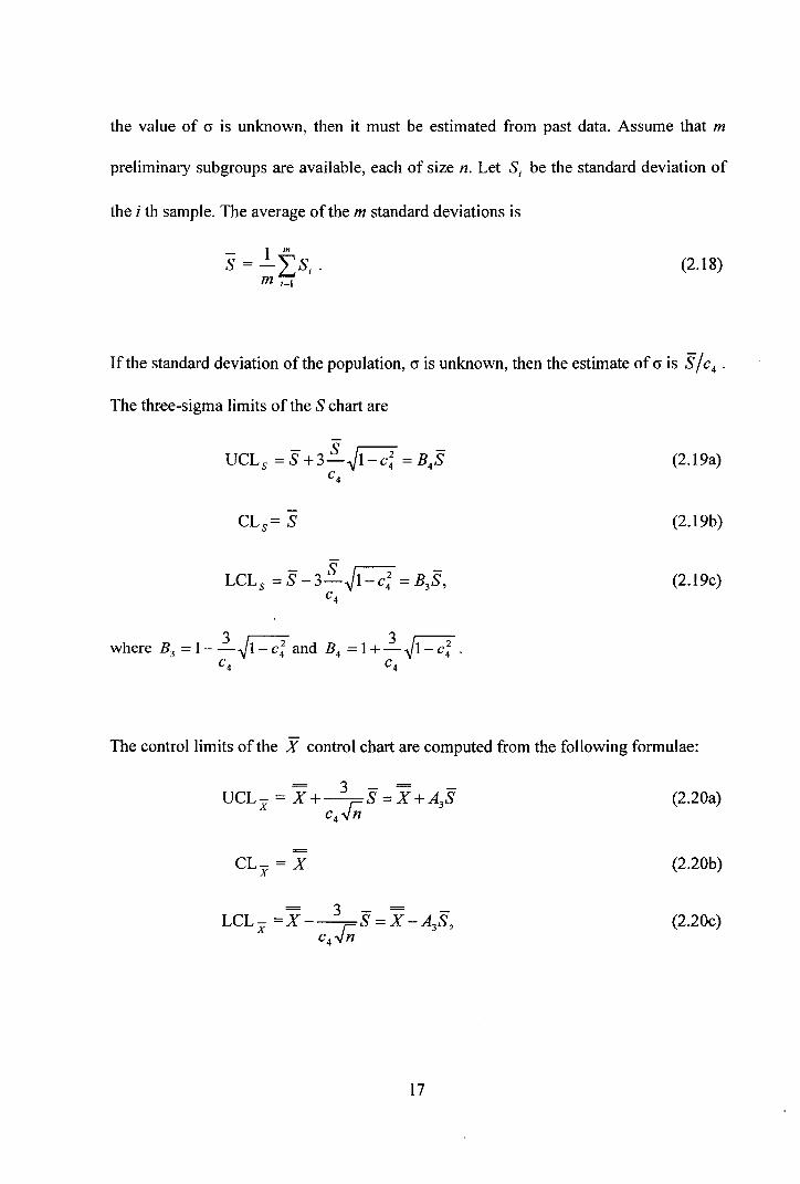
the value of a is unknown, then it must be estimated from past data. Assume that m
preliminary subgroups are available, each of size n. Let S; be the standard deviation of
the i th sample. The average of them standard deviations is
(2.18)
If the standard deviation of the population, a is unknown, then the estimate of a is S / c 4 •
The three-sigma limits of the S chart are
(2.19a)
CLs= S (2.19b)
(2.19c)
The control limits ofthe X control chart are computed from the following formulae:
(2.20a)
CL- =X X
(2.20b)
= 3 = LCL- =X---S=X-AS x r 3 ' c4 -vn
(2.20c)
17
3 where A3 =
1 . Values of constants A3 , B3 and B 4 for various sample sizes, n are
c4 vn
given in Table A.1 in Appendix A.
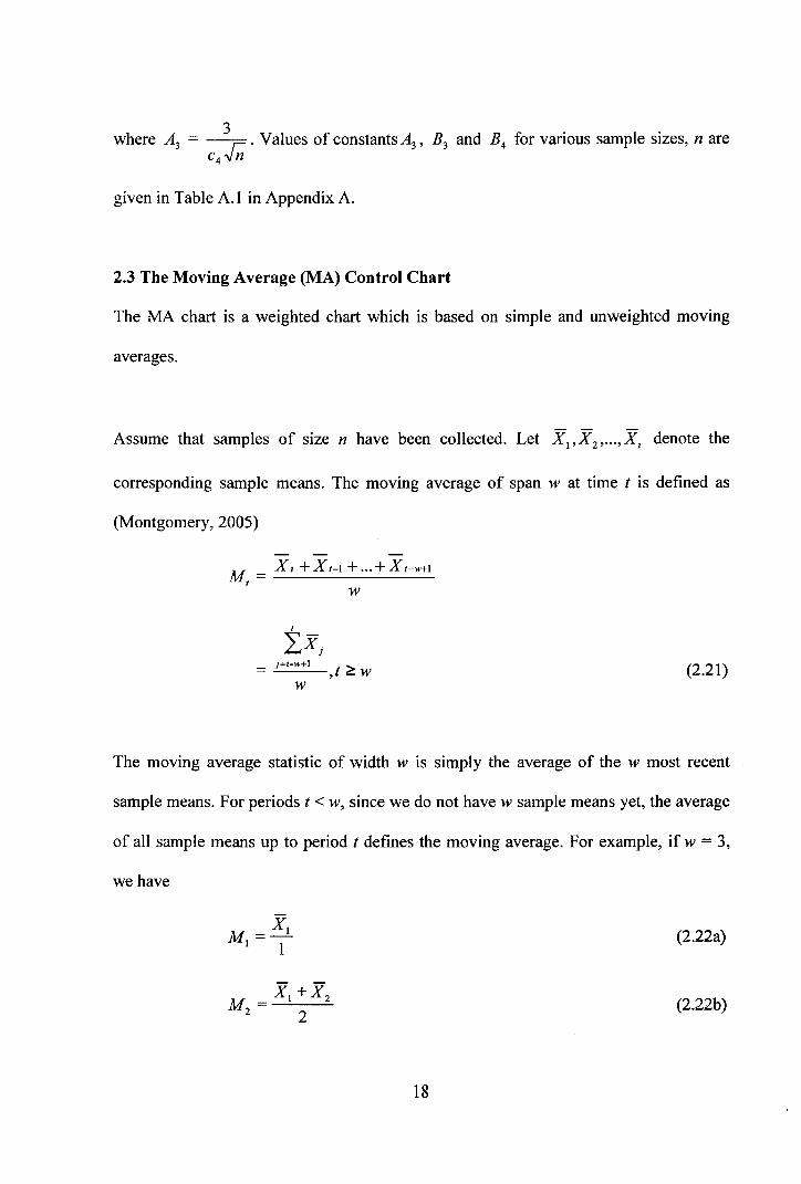
2.3 The Moving Average (MA) Control Chart
The MA chart is a weighted chart which is based on simple and unweighted moving
averages.
Assume that samples of size n have been collected. Let X"X2 , ••• ,X, denote the
corresponding sample means. The moving average of span w at time t is defined as
(Montgomery, 2005)
M =X, +Xr-1 + ... +Xr-w+1 t
w
_ j=t-w+1 ,t;::: w (2.21) w
The moving average statistic of width w is simply the average of the w most recent
sample means. For periods t < w, since we do not have w sample means yet, the average
of all sample means up to period t defines the moving average. For example, if w = 3,
we have
x1 M=-
1 1 (2.22a)
(2.22b)
18

and
M =X, +X,_1 +X,_2 >
3 I ,f- • 3
(2.22c)
At time t, the moving average is updated by dropping the oldest sample mean and the
newest one is added to the set The variance of the moving average statistic M, is
1 (- - - ) Var(M,) = -2
Var X, +X1-1 + ... +Xt-w+! . w
If X, is the t th sample mean, then
(-) - cr2 Var X, = Var(x)=-.
n
Thus,
1 , cr2 crz Var(M,)= -
2 L - =-
w ;~t-w+! n nw
and the standard deviation of M, is cr M = cr I ,J;;;. I
The three-sigma control limits for the moving average chart are
= 3cr UCL =X+--M, r-
-.JnW
CL =X M,
= 3cr LCL =X---
M, r- ' -vnw
19
(2.23)
(2.24)
(2.25)
(2.26a)
(2.26b)
(2.26c)

where n denotes the sample size. Note that for period t < w, w is replaced with t in
Equations (2.26a) and (2.26c).
If the value of a is unknown, it can be replaced with a= R I d 2 or a= S I c4 ,where R
and S denote the average sample range and average sample standard deviation,
respectively, both estimated from an in-control historical data set. In practice, R is
considered for n < 10 while S otherwise (Montgomery, 2005).
In general, the magnitude of a shift of interest and w are inversely related, i.e., smaller
shifts would be guarded against more effectively by longer-span moving average, w, at
the expense of a quick response to large shifts (Montgomery, 2005).
20
CHAPTER3
A REVIEW ON SOME ROBUST CONTROL CHARTS
3.1 The Robust X Q - RQ Charts
When a process is first subjected to statistical quality control, a normal procedure is to
collect 20-40 subgroups of observations and then to construct control charts such as X
and R charts with limits determined by the data. These control charts are then used to
detect problems in the process, such as outliers or excessive variability in the sample
means that may be due to a special cause. Rocke (1989 and 1992) proposed a new
method of determining the control limits for X and R charts that result in easier
detection of outliers and greater sensitivity to other forms of out-of-control behavior
when outliers are present. The control limits for these charts, i.e., the X Q and RQ charts
are determined from the average subgroup interquartile range.
This new charting method will be appropriate when the following conditions are
satisfied (Rocke, 1992):
1) The control limits are to be established from the data at hand, rather than from a
known value of cr, the process standard deviation. This will usually be the case when
a process is newly brought under statistical quality control procedures.
2) There is a possibility of outliers in the data within the subgroup. If the distribution is
known to be normal (which would rarely be the case), then standard procedures such
as X and R charts will suffice. The terms 'outlier' is used to mean an observation
that is unusually far from the rest of the data. This may indicate that the particular
21
data point was drawn from a different population or that a sporadic special cause
was operating.
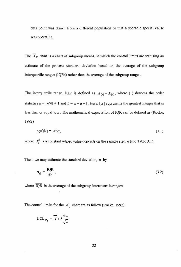
The X Q chart is a chart of subgroup means, in which the control limits are set using an
estimate of the process standard deviation based on the average of the subgroup
interquartile ranges (IQRs) rather than the average of the subgroup ranges.
The interquartile range, IQR is defined as X(b)- X(a)' where ( ) denotes the order
statistics a = [ n/4] + 1 and b = n - a + I . Here, [ x ] represents the greatest integer that is
less than or equal to x. The mathematical expectation of IQR can be defined as (Rocke,
1992)
E(IQR) = dfcr, (3.1)
where df is a constant whose value depends on the sample size, n (see Table 3.1 ).
Then, we may estimate the standard deviation, cr by
_ IQR (JQ- -Q-,
d2 (3.2)
where IQR is the average of the subgroup interquartile ranges.
The control limits for the X Q chart are as follow (Rocke, 1992):
A
= cr UCL- = X+3 Q
Xg -Jn
22
CL- =X Xg
= O"o LCL- = X -3--
xQ I -vn
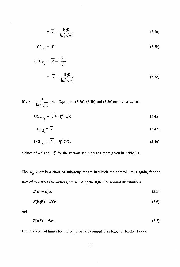
If Af = ( Q3
')'then Equations{3.3a), (3.3b) and (3.3c) can be written as d2 ..,;n
CL- =X Xg
LCLx =X -AfiQR. Q
Values of df and Af for the various sample sizes, n are given in Table 3.1.
(3.3a)
(3.3b)
(3.3c)
(3.4a)
(3.4b)
(3.4c)
The RQ chart is a chart of subgroup ranges in which the control limits again, for the
sake of robustness to outliers, are set using the IQR. For normal distributions
(3.5)
E(IQR) = df cr (3.6)
and
(3.7)
Then the control limits for the RQ chart are computed as follows (Rocke, 1992):
23

(3.8a)
(3.8b)
(3.8c)
where d2 and d3 are standard constants (Wadsworth et al., 1986).
Let
(3.9)
(3.1 0)
and
(3.11)
then the control limits for the RQ chart can be written as (Rocke, 1992)
(3.12a)
(3.12b)
LCL~ = DfiQR. (3.12c)
Values of dfR, Df and Df for the various sample sizes are given in Table 3 .1.
24