1 components of variance - mcgill university components of variance ... pairs of identical twins...

BIOS602: Components of variance; combining information; meta-analyses; extra-binomial/poisson variation [2011.03.12]

1 Components of Variance

Researchers are often interested in de-composing observable variation into twoor more components or sources. Examples include ...

• quantifying , in genetic or family studies, how much of the variationin a quantitative trait (e.g. height, blood pressure, cholesterol) is truebetween-family variation, how much is true ’between-individual-within-same-family’ variation, and how much is real within-individual variationor measurement error. We will examine three such studies.

In the first (see the 1990 Time magazine story1

Canadian researchers [using U. Laval students as subjects –being in the study was the student’s summer job] fed twelvepairs of identical twins 1,000 calories above their normal dailyintake for 84 days out of a 100- day period. Weight gains rangedfrom 4 kg to 13 kg (9 lbs. to 29 lbs.). But the difference inthe amount gained was much less between twins than betweensubjects who were not siblings. Concludes Claude Bouchard,a professor of exercise physics at Quebec’s Laval University:”It seems genes have something to do with the amount yougain when you are overfed.” Some sets of twins transformedthe extra calories into mostly fat, while others converted theminto lean muscle.

The second was motivated by the observation “anatomical, physiological,and epidemiological data indicate that there may be a significant geneticcomponent to prolonged time with and recurrent episodes of otitis mediain children”. As its objective, it sought

to determine the genetic component of time with and episodesof middle ear effusion and acute otitis media (AOM) during thefirst 2 years of life’.

The third uses Galton’s family stature (height) data to examine between-and within-family differences in adult heights.

1“Chubby? Blame those genes: Heredity plays the pivotal role in weight control”http://www.time.com/time/magazine/article/0,9171,970266,00.html

Chubby? Bbrne ( Heredity plays the pivotal rvle in weight control

I t h a long been clear that people's wc&t is determined by a balance of he-

huviet e l k t ? Two reports in last week's New Eqfand Jownal of Medicine tip the

I d ig a d life-style. But which exerts the , i

scales finnty ta rud genetic makeup. In one investigation. researchers from 1

the US. a d Sweden matyzd eight and I

height rrcordr from the Swedish Adop t M r i n Study ot wng . R d n s data on 247 identical and 426 f n t e d pain of twim. the cum found that siblinp end up with similar body wighu whcthcr 01 not they uc raised in diflerrnt families and that they are much rime likell, to grm up lookins like their naturd puenu than

Wopyright. 1990. by the Musrhusc~ts Medical Society

Volume 322 M A Y 24. 1990 N u n \ t ) r r ' L I

THE RESPONSE TO LONG-TERM OVERFEEDING IN IDENTICAL TWINS CLAUDE BOUCHARD, PH.D., ANCEI.O '~REMBLAY, PH.D.,.IEAN-PIERRE DESPRBS, pH.[)., I\NDR~? NAIIF.AU. h f . D . , PAUL J. LUPIEN, M.D.. PH.D., GERMAIN TII~RIAIII.T, M . D . , JEAN I)I~ssA[~I.T, M.D.. SI.I.AI. ~ ~ O O R J A N I , Ptt . I ) . ,

SYI.VIE PINAULT, M.D., AND GIIY FOIIRNIER, B.Sc .

Abrtnct We undertook this study to determine whettmf Itme ere dfferences in the responses of diflerent persw to kng.term overieeding and to assess the possibikty that

are invdved in such differences. After a two- week base-line period. 12 pairs of young adult mde monozygotic twins were oveded by 4.2 W (1000 kcal) psr dry, 6 days a week, for a total of 04 days during a 1 W y p e w . The total excess amount each man consumed was

estimated subcutaneous fat, with abwt three times more variance among pairs than within pain (r - 0.5). After ad- justment for the gains in fat mass. the within-pair similarity was particularty evident with respect to the changes in regional fat distribution and amount of abdominal visceral fa1 (P<0.01). wlth about six thmm as much variance among pairs as within pairs (r - 0.7).

We condude lhat the most l i k e edanation for the 353 MJ (84.000 kcal). inlrapair similarity in the adaptation tb &-term overfeed-

During overfeeding. individual charwes in body comfm ing and for the varialions in weight aain md fat distribution sition a d topograp6i of fat deposit& varied &s&-. ariong the pahs of twins is $at -- factors are in- abiy. mean weight gain was 8. i kg, bui iiis far* wss \rib+&. T t i i ~6 rij g~-<er~ the tei&ii* :G s:~-e e i i q j as 4.3 to 13.3 kg. The similarity within each pair in the re- either fat or lean tissue and the various determinants ol the sponse to wedeeding was sigrwficant (Pc0.05) with re- re~tlng expenditure of energy. (N Engl J Mad 1990; spect to body weight. percentage of fat. fat mass. and 3221477-82.)

Chubby? Bbrne ( Heredity plays the pivotal rvle in weight control

I t h a long been clear that people's wc&t is determined by a balance of he-

huviet e l k t ? Two reports in last week's New Eqfand Jownal of Medicine tip the

I d ig a d life-style. But which exerts the , i

scales finnty ta rud genetic makeup. In one investigation. researchers from 1

the US. a d Sweden matyzd eight and I

height rrcordr from the Swedish Adop t M r i n Study ot wng . R d n s data on 247 identical and 426 f n t e d pain of twim. the cum found that siblinp end up with similar body wighu whcthcr 01 not they uc raised in diflerrnt families and that they are much rime likell, to grm up lookins like their naturd puenu than

Wopyright. 1990. by the Musrhusc~ts Medical Society

Volume 322 M A Y 24. 1990 N u n \ t ) r r ' L I

THE RESPONSE TO LONG-TERM OVERFEEDING IN IDENTICAL TWINS CLAUDE BOUCHARD, PH.D., ANCEI.O '~REMBLAY, PH.D.,.IEAN-PIERRE DESPRBS, pH.[)., I\NDR~? NAIIF.AU. h f . D . , PAUL J. LUPIEN, M.D.. PH.D., GERMAIN TII~RIAIII.T, M . D . , JEAN I)I~ssA[~I.T, M.D.. SI.I.AI. ~ ~ O O R J A N I , Ptt . I ) . ,

SYI.VIE PINAULT, M.D., AND GIIY FOIIRNIER, B.Sc .

Abrtnct We undertook this study to determine whettmf Itme ere dfferences in the responses of diflerent persw to kng.term overieeding and to assess the possibikty that

are invdved in such differences. After a two- week base-line period. 12 pairs of young adult mde monozygotic twins were oveded by 4.2 W (1000 kcal) psr dry, 6 days a week, for a total of 04 days during a 1 W y p e w . The total excess amount each man consumed was

estimated subcutaneous fat, with abwt three times more variance among pairs than within pain (r - 0.5). After ad- justment for the gains in fat mass. the within-pair similarity was particularty evident with respect to the changes in regional fat distribution and amount of abdominal visceral fa1 (P<0.01). wlth about six thmm as much variance among pairs as within pairs (r - 0.7).

We condude lhat the most l i k e edanation for the 353 MJ (84.000 kcal). inlrapair similarity in the adaptation tb &-term overfeed-

During overfeeding. individual charwes in body comfm ing and for the varialions in weight aain md fat distribution sition a d topograp6i of fat deposit& varied &s&-. ariong the pahs of twins is $at -- factors are in- abiy. mean weight gain was 8. i kg, bui iiis far* wss \rib+&. T t i i ~6 rij g~-<er~ the tei&ii* :G s:~-e e i i q j as 4.3 to 13.3 kg. The similarity within each pair in the re- either fat or lean tissue and the various determinants ol the sponse to wedeeding was sigrwficant (Pc0.05) with re- re~tlng expenditure of energy. (N Engl J Mad 1990; spect to body weight. percentage of fat. fat mass. and 3221477-82.)

• quantifying, in ‘measurement studies’, the amount of measurementerror, and expressing it as a coefficient of variation (CV) or reliabilitycoefficient or Intra Class Correlation Coefficient (ICC).

1


Data analysis

Traditionally, the variance components have been estimated using ‘methodsof moments’ estimators applied to the mean squares calculated in classicalANOVA tables based on a 1-way (or several-way) mixed or random effectsmodel. As statistical computing had become easier, we can now more easilyand more flexibly estimate these parameters using a number of approachesand software packages.

But it is best to begin with the classical way. So, following this page, JHhas pasted in here 5 pages (numbered 2-6) of orientational material on mea-surement statistics from a measurement course for physical and occupationaltherapy students. These students had had limited exposure to statistical con-cepts in general, and to ‘ANOVA’ in particular; this lack of familiarity with‘classical’ ANOVA2 does not seem to be limited to such students: many mod-ern ‘regression and anova’ courses skip the ‘anova’ altogether, since many ofthe statistical tests (and anova tests were traditionally the focus) can be car-ried out within a more general regression framework. But in our focus onestimation, and in particular on variance-estimation, we have something tolearn from the classical anova tables and calculations, and particularly froma concept that is seldom taught within a regression-only course, namely theExpected Mean Square or EMS. It was mainly used in classical anova to il-lustrate which Mean Squares should be used in an F test to test which nullhypotheses.

Opposite is an excerpt from an older text, showing the EMS for the twosimplest ‘1-way anova’ models. We will be more interested in the version wherethe α’s are random rather than fixed, but to make it easier, the orientationalmaterial starts with the fixed effects model. The anova calculations are thesame in both the fixed and random-effects models: it is the use of the Means-squares that differs in the two models.

2By ‘classical’ I mean the calculations could be easily done by a hand calculator; thedata structure was nicely balanced and the data could be laid out in rows and columns, orin a higher-dimensional array, with no missing values, no other explanatory , etc.

ANALYSIS OF VARIANCE AND EXPECTED MEANSQUARES FOR THE ONE-WAY CLASSIFICATION

Model: yij = µ+ αi + εij ; (i = 1, 2, . . . , k; j = 1, 2, . . . , ni; n. =∑i ni)

Fixed Effects: α1, . . . αk fixed & unknown; 1, 2, . . . , k exhaustive;∑i αi = 0.

Random Effects: α1, . . . αk: sample from larger no. of α’s, with α ∼ N(0, σ2B)

εij ∼ N(0, σ2W ), i.i.d. B: Between; W: Within.

Source of Degrees of Sum of Squares Mean TestVariation Freedom Square Statistic

Between k − 1 S1 =∑i

∑j(yi − y..)

2 s21 = S1

k−1 F =s21s20

groups

Within n. − k S0 =∑i

∑j(yij − yi)

2 s20 = S0

n.−kgroups

Total n. − 1 S =∑i

∑j(yij − y..)

2

Source of Degrees of Mean Expected Mean Square (EMS) for model with...Variation Freedom Square

Fixed Effects Random Effects

Between k − 1 s21 σ2W +

∑i niα

2i

k−1 σ2W + 1

k−1 (n. −∑n2i

n.)σ2B *

groups

Within n. − k s20 σ2W σ2

W

groups

Total n. − 1

* With equal n’s, EMS = σ2W + nσ2

B ; with unequal n’s, EMS > σ2W + nσ2

B .

2


Introduction to Measurement Statistics 2 - First, a General Orientation to ANOVA and its primary use, namely DE-COMPOSITION OF OBSERVED (EMPIRICAL) VARIATIOPJ testing differences between p's of k ( 22 ) different groups.

DATA:

Group 1 2 1 k

Subject 1 Y11 2

j Yij

n Y kn

- - - - Mean Y1 Y2 Yi Yk

Variance s2, s22 s2k

MODEL

o refers to the variation (SD) of all possible individuals in a group; It is an (unknowable) parameter; it can only be ESTIMATED.

Or, in symbols ...

TOTAL Sum - - BETWEEN Groups + W I T m Group of Squares Sum of Squares Sum of Squares

ANOVA TABLE

Sum of Degrees Mean F P-Value Squares of Freedom Square Ratio

SOURCE SS df MS MSerTwrrN prob(>~) MS WITHIN

(= SS /df)

BETWEEN xx.x k-1 xx.x x.xx 0.xx WITHIN xx.x k(n-1) xx.x

LOGIC FOR F-TEST (Ratio of variances) as a test of

UNDER HO

Means, based on samples of n, (T

2 should vary around p with a variance of

Thus, if Ho is true, and we calculate the empirical variance of the k different Ti's, it 02 should give us an unbiased estimate of - n

.

3


Introduction to Measurement Statistics 3 - 02 Z['i - 'I2 is an unbiased estimate of - k- 1 n

How ANOVA can be used to estimate Components of Variance used in quantifying Reliability.

The basic ANOVA calculations are the same, but the MODEL underlying them is i.e. Z[yi - 'I2 is an unbiased estimate of o2 different. First, in the more common use of ANOVA just described, the groups can

k- 1 be though of as all the levels of the factor of interest. The number of levels is necessarily finite. The groups might be the two genders, all of the age groups, the 4 blood groups, etc. Moreover, when you publish the results, you explicitly identify

i.e. "[" - 'I2 = M S B E ~ ~ is an unbiased estimate of o2 k- 1 the groups.

Whether or not Ho is true, the empirical variance of the n (within-group) values C[?.. - 7.12

11 Y i l to Yin i.e. should give us an unbiased estimate of o2 n- 1

C[Y.. - 7.12 S 2 . = 11 ' is an unbiased estimate of o2 n- 1

so the average of the k diferent estimates,

is also an unbiased estimate of o2

i.e. ZZ[Yii - yi12 = M S W ~ is an unbiased estimate of d k[n-1]

When we come to study subjects, and ask "How big is the intra-subject variation compared with the inter-subject varaition, we will for budget reasons only study a sample of all the possible subjects of interest. We can still number them 1 to k, and we can make n measurements on each subject, so the basic layout of the data doesn'y change. All we do is replace the word 'Group' by 'Subject' and speak of BETWEEN- SUBJECT and WITHIN-SUBJECT variation. So the data layout is ... DATA:

Subject

Measurement

j Yij

n Y kn

THUS, under Hg, both M S B E ~ ~ and M S W I T ~ are unbiased estimates of - - - - Mean estimates of o2 and so their ratio should, apart from sampling variability, be 1. Y1 Y2 Yi Y k

IF however, Ho is not true, M S B E ~ ~ will tend to be larger than MSWITHIN, Variance s22 since it contains an extra contribution that is proportional to how far the p's are s2k

from each other.

In this "non-null" case, the M S B E ~ E N is an unbiased estimate of MODEL

and so we expect that, apart from sampling variability, the ratio MSBETWEEN MS WITHIN

The model is different. There is no interest in the specific subjects. Unlike the critical labels "male" anf "female", or "smokers", "nonsmokers" and "exsmokers" to identify groups of interest, we certainly are not going to identify subiects as Yves, Clairi:, Jean, Anne, Tom, Jim, and Hany in the publication, and nobody would be fussed if in the dataset we used arbitrary subject identifiers to keep track of which

should be greater than 1. The tabulated values of the F distribution (tabulated measurements were made on whom. we wouldn't even care if the research assistant under the assumption that the numerator and denominator of the ratio are both lost the identities of the subjects -- as long as we know that the correct measureiits estimaes of the same quantity) can thus be used to assess how extreme the observed go with the correct subject! F ratio is and to assess the evidence against the Ho that the p's are equal.

.

4


Introduction to Measurement Statistics 4 - The "Random Effects" Model uses 2 stages: DE-COMPOSITION OF OBSERVED (EMPIRICAL) VARIATION

(1) random sample of subjects, each with hisher own p (2) For each subject, series of random variations around hisher p

TOTAL Sum - - Notice the diagram has considerable 'segregation' of the measurements on different BETWEEN Subjects + WITHIN Subjects individuals. There is no point in TESTING for (inter-subject) differences in the p's. of Squares Sum of Squares Sum of Squares The task is rather to estimate the relative magnitudes of the two variance components 2,and dw. ANOVA TABLE (Note absence of F and P-valzle Colz~mns)

Sum of Degrees Mean What the Mean SquaresofFreedom Square S q u a r e i s a n

p's for Universe of Subjects h

estimate of* SOURCE SS df MS

(= SS /do

BETWEEN Subjects xx.x k-1 XX.X $ , + n $ B

WITHIN Subjects xx.x k(n-1) xx.x 2W

YVS = I \ ACTUAL ESTIMATION OF 2 Variance Components

refers to the SD of the universe of p's ; If is an B unknowable parameter and can only be ESTIMATED

MS BETWEEN is an unbiased estimate of $ + n $

MSWITHIN is an unbiased estimate of $

By subtraction ... MSBETWEEN - MS WITHIN is an unbiased estimate of n $

refers to the variation (SD) of all possible measurements on a sudject WIt is an (unknowable) parameter; it can only be ESTIMATED.

MSBETwEeN - wlTHIN is an unbiased estimate of dB n Or, in symbols ...

Yij = p i + e i j = p f (pi--p) f Eij This is the definitional formula; the computational formula may be different.

* Pardon my ending with a preposition, but I find it difficult to say otherwise. These parameter combinations are also called the "Expected Mean Squares". They are the long-run expectations of the MS statistics As Winston Churchill would say, "For the sake of clarity, this one time this wording is something up which you would put".

.

5


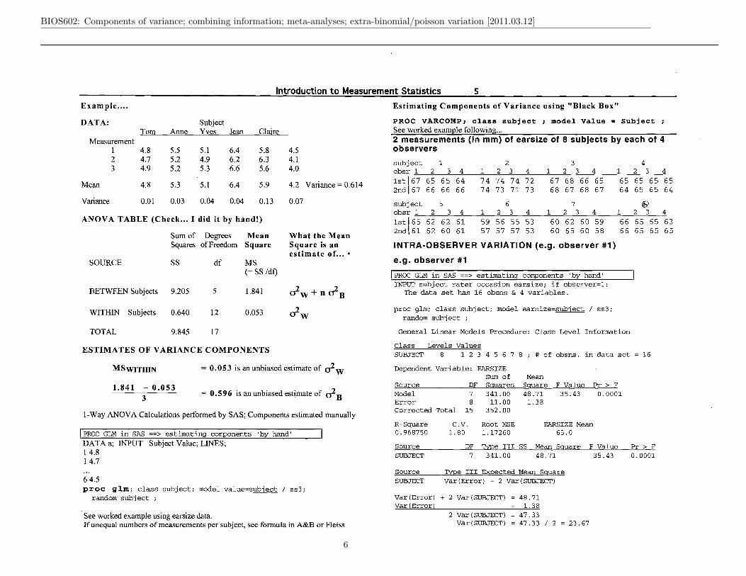
Introduction to Measurement Statistics 5 - Example .... Estimating Components of Variance using "Black Box"

DATA: Subject Tom Anne Yves Jean Claire

Measurement 1 4.8 5.5 5.1 6.4 5.8 4.5

Mean

P R O C VARCOMP; class subject ; model Value = Subject ; See worked example following ... - 2 measurements (in mm) of earsize of 8 subjects by each of 4 observers subject 1 2 3 4 obsrl 2 3 4 1 2 3 4 1 2 3 4 1 2 3 4

Variance 0.01 0.03 0.04 0.04 0.13 0.07

ANOVA TABLE (Check ... I did it by hand!)

subject 5 6 7 o b s r 1 2 3 4 1 2 3 4 1 2 3 4

8 1 2 3 4

lst165 62 62 61 59 56 55 53 60 62 60 59 66 65 65 63

Sum of Degrees Mean What the Mean 2ndi61 62 60 61 57 57 57 53 60 65 60 58 66 65 65 65

Squares of Freedom Square Square is an INTRA-OBSERVER VARIATION (e.g. observer # I ) estimate of . . . *

SOURCE S S d f MS e.g. observer #1 (= SS Idf) [ PROC GLM in SAS ==> estimating components 'by hand' I

INPUT subject rater occasion earsize; if observer=l; BETWEEN Subjects 9.205 5 1.841 d w + n $ B The data set has 16 obsns & 4 variables.

WITHIN Subjects 0.640 12 0.053 d w proc glm; class subject; model earsize=subject / ss3; random subject ;

TOTAL 9.845 17 General Linear Models Procedure: Class Level Information

ESTIMATES OF VARIANCE COMPONENTS Class Levels Values SUBJECT 8 1 2 3 4 5 6 7 8 ; #ofobsns.indataset=16

M ~ W I T H I N = 0.053 is an unbiased estimate of $ Dependent Variable: EARSIZE Sum of Mean

1.841 - 0 .053 Source DF Swares Suuare F Value Pr > F

3 = 0.596 is an unbiased estimate of $& Model 7 341.00 48.71 35.43 0.0001 Error 8 11.00 1.38 Corrected Total 15 352.00 1-Way ANOVA Calculations performed by SAS; Components estimated manually

IPROC GLM in SAS ==> estimating components 'by hand' DATA a; INPUT Subject Value; LINES;

I 1 4.8 1 4.7 . . . 6 4.5 proc glm; class subject; model value=subject / ss3; random subject ;

See worked example using earsize data. If unequal numbers of measurements per subject, see formula in A&B or Fleiss

R-Square C.V. Root MSE EARSIZE Mean 0.968750 1.80 1.17260 65.0

Source DF Type I11 SS Mean Square F Value Pr > F SUBJECT 7 341.00 48.71 35.43 0.0001

Source m e I11 Expected Mean Square SUBSECT Var (Error) + 2 Var (SUBSECT)

Var(Error) + 2 Var(SUBJECT) = 48.71 Var (Error) = 1.38

2 Var(SUBSECT) = 47.33 Var(SUBJECT) = 47.33 / 2 = 23.67

.

6


Introduction to Measurement Statistics 6 - 1 Estimating Variance components using PROC VARCOMP in SAS 1 Proc varcomp; class subject ; model earsize = subject ;

Variance Components Estimation Procedure: Class Level Information

Class Levels Values

SUBSECT 8 1 2 3 4 5 6 7 8 ; # obsns in data set = 16

MIVQUE(0) Variance Component Estimation Procedure

Estimate Variance Component EARSIZE

Var ( SUBSECT) Var(Error)

ICC (Fleiss § 1.3)

1 -sided 95% Confidence Interval (see Fleiss p 12)

df for F in CI: (8-1)= 7 and 8

so from Tables of F distribution with 7 & 8 df, F = 3.5

So lower limit of CI for ICC is

EXERCISE: Cany out the estimation procedure for one of the other 3 observers.

.

7


Applying this 1-way model to Bouchard’s ‘chubby genes’ data:

'4

-! w. incr. twin 13.3 11.1 8.2 6.1 7.9 7.1 6.9 6.5 6.7 7.3 6.5 5.4 ybar: 8.08 , Jw.incr.twin4 1 1 12.9 9.6 11.4 7.7 6.9 8 8 8.8 4.3 5.3 7.1 I var: 5.54 $ i,. s.d.: 2.35

I.: ANOVA TABLE

df Mean Sq F ! B 1 w Poplru + , . W.58 11 8.87 3.56 ' W / n Poplns 29.93 12 2.49 ~ L u ii ins1 23 5.54

weight increase

twin palr

.

8


From this anova table and the concept of Expected Mean Squares3, wecan, by the method of moments, get estimates of the separate components ofthat parameter combination.

Quantifyina Reliability 3 - ICC's (Portnoy and Wilkins) ( I ) multiple (unlabeled) measurements of each subject

model: weight gain for person j in family i = p + p + ai + eij

(2) same set of raters measure each subject; raters thought of as a random sample of all possible raters. 1-way Anova and Expected Mean Square (EMS)

(3) as in (2), but these raters studied are the only raters of interest ............................................................................

Source Sum d. f Mean Expected Mean Square of Sq Square

( I ) multiple (unlabeled) measurements o f each subject Between (families) 99 11 9.0 0 2 n n + kg 0%-n

Error(~ithin families) 30 12 2.5 0211emxn

ICC =

Model for obsemed data:

subject i, measurement j] = p + q + ~ i j

EXAMPLE 1

This example is in the spirit of the way the ICC was first used, as a measure of the greater similarity within families than between families: Study by B0uchm-l (NFJM) on weight gains of 2 members from each of 12 families: It is thought that there will be more variation between members of different families than between members of the same family: family (genes) is though to be a large source of variation; the two twins per family are thought of as 'replicates' from the family and closer to each other (than to others) in their responses. Here the "between" factor is familv i.e. families are the subjects and the two twins in the family are just replicates and they don't need to be labeled (if we did label them 1 and 2, the labels would be arbitrary, since the two twins are thought to be 'interchangeable'. (weight gain in Kg over a summer)

----

Total

In our example, we measm k=2 members from each family, so ko is simply 2

[if the k's are unequal, ko is somewhat less than the average t.. ko = average k - (variance of kls) / (n times average k) ... see Fleiss page 101

Estimation of parameters that go to make up ICC

2.5 is an estimate of G2nermrw

9.0 is an estimate of 02*mr* + 2 O h t w e a ---------------------i-----------------------------------

:. 6.5 is an estimate of 2 oh tween

6.5 - is an estimate of 2

is an estimate of ICC = 02between b%etween + 02error

3Think of the EMS for the row in question as the combination of parameters which is(mean-unbiasedly) estimated by the mean square in that row.

.

9


You will often find in statistical ‘cookbooks’ that the ICC, and other concepts –such as those behind the kappa statistic – are defined by the simplest and user-friendliest computational formula its estimator. But biostatisticians shouldalways distinguish between the definition of a parameter and its estimator.Typically the parameter involves Greek letters (some teachers used upper classRoman ones) and the estimator uses data, and the estimate is often denotedby a Greek letter with hat on it, or the lower-case Roman letter equivalentof the upper-case one. In the ‘by hand’ days, there was the same issue withrespect to the definitional formula for a variance or standard deviation versusthe user-friendliest computational formula for an estimator of it.

COMPUTATIONAL Formula for " 1-way" ICC

MSbetween - MSwithin ko

MSbetween - MSwithin + MS within ko

- MSbetween- MSwithin - MS between + &-1)MSwithin

is an estimate of the ICC

Quantifying Reliability 4

Increasing Reliability by averaging several measurements

In l-way model: Yij=P + Ui + eij

where var[ai ] = o2ktween subjects ; vafleij ] = Cf21*-rl*

Then if we average k measurements, i.e.,

ybSi = + ai + e b ~ i

then , 62",,. VW 1 = a2between

1 k

Notes: s o Icc[k] = Slreiner and Nonnan start on page 109 with the 2-way anova far inter-obsemer 62wenorw

variation. There are mistakes in their depiction of the S S e m on p 110 [it should be 02between + k (6-6)2+(4-4)2+(2-1)2 +...(8-)2 =lo. If one were to do the calculations by hand, one usually calculates the SStotal and then obtains the S S m r by subtraction] They then mention the I-way case, which we have discussed above, as "the

ob&er nested within subjeci" on page 112 Fleiss gives methods for calculating CI's for ICC's.

EXAMPLE 2: INTRA-OBSERVER VARIATION FOR 1 OBSERVER

Computations performed on earlier handout...

An estimated 94% of obseaved variation in earsize measurements by this observer is 'real' .. i.e. reflects true between-subject variability.

This is called "Stepped-Up" Reliability.

Note that I say 'an estimated 94% ...". I do this because the 94% is a statistic that is subject to sampling variability (94% is just a point estimate or a 0% Confidence Interval). An interval estimate is given by say a 95% confidence interval for the true ICC (lower bound of a 1-sided CI is 82% ... see previous handout)

.

10


≥ 3 components of variance:when human (or other fallible) raters are involved

The 64 ear-length measurements below were taken by 4 raters (a subset of thestudents) who measured 8 subjects (6 other students, as well as the teachersSharon Wood-Dauphinee and James Hanley) in a (physical and occupationaltherapy) class on measurement in rehabilitation. The choice of ’objects’ mea-sured was prompted by the article Why do old men have big ears? [authorJames A Heathcote, general practitioner] in the Christmas Edition of theBJM in December 1985, and some follow-up letters the following March – seeResources.

Quantifying Reliability 5 ICC's (Portnog and Wilkins). (2) same set of raters measure each subject; raters thought of ar a random s a v l e of

allpossible raters. Model

y for subject 2, latea I1

qd 4- y for subject 2, rater I I

"4 y for subject 3, rater I1 +-+ y for subject 3, rater I I

etc ...

ESTIMATING INTER-OBSERVER VARIATION from occas ion=l;

PROC GLM in SAS ==> estimating components 'by hand' I INPUT subject rater occasion earsize; if occasion=l; (32 obsns)

proc glm; class subject rater; model earsize=- rater / ss3; random subject rater;

General Linear Models Procedure: Class Level Information

Levels Val= SUBJECT 8 1 2 3 4 5 6 7 8 RATER 4 1 2 3 4 Number of observations in data aet = 32

Sum of Mean re F Value Pr > E

Model 10 764.500 76.45 78.80 0.0001 !ZJZor 21 20.375 0.91 Corrected Total 31 784.875

re F Value Pr z E SUBJECT 7 734.875000 104.98 108.20 0.0001 RATER 3 29.625000 9.87 10.18 0.0002

2 2 2 o ~ ~ b j c c ~ dl;lters

From 2- way data layout (subjects x Raters)

estimate o ~ * * ~ ~ ~ ~ ~ , d2nramsn and (r2n-n by 2-way ANOVA Substitute variance estimates in appropriate ICC form

e.g. 2 measurements (in mm) of earsize of 8 subjects by each of 4 observers

subject 1 2 3 4 obsr 1 2 3 4 1 2 3 4 1 2 3 4 1 2 3 4 1st 67 65 65 64 74 74 74 72 67 68 66 65 65 65 65. 65 2nd I 67 66 66 66 74 73 71 73 68 67 68 67 64 65 65 64

subject 5 6 7 6

1st 65 62 62 61 59 56 55 53 60 62 60 59 66 65 65 63 2nd 61 62 60 61 57 57 57 53 60 65 60 58 66 65 65 65 0bsi"34 1 2 "

SUBJECT Var(Error) + 4 Var(SUBJECT) RATER Var(Error) + 8 Var(RATER) So ... solving 'by hand' for the 3 components ...

==> Y a r . ( S ~ % ~ C T . l .. F-.;IP.~.,P.I..~.-~~..:..~C...P.~ Var(Error) + 8 Var (RATER) = 9.87

Estimating Variance components using PROC VARCOMP in SAS I proc varcomp; class subject rater; model earsize = subject rater;

Estimate

Var (SUBJECT) 26.00 Var (RATER) 1.11 Var (Error) 0.97

Quantifying Reliability 6

ICC: "Raters Random" (Fleiss 5 I .5.2)

Var (SUBJECT) 26.00 = ..................................... = -------------- = 0.93 Var(SUBJECT) + Var(RATER) + Var(Error) 26.00+1.11+0.97

df for F in CI: (8-1)= 7 and v' , where

so from Tables of F distribution with 7 & 8 df, F = 3.5

So lower limit of CI for ICC is

ICC: If use one "flxed observer (see Fleiss p 23, strategy 3)

lower limit of 95% 1-sided CI (eqn 1.49: F = 2.5 ; 7 & 7x3=21 df)

USING ALL THE DATA SIMULTANEOUSLY

(can now estimle subject x Rater interaction .. i.e extent to which raters 'reverse themselves' with different subjects)

- - - - - - - - - - - - - - - - - - -

@omponents of variance when use both measurements (all 64 obsns) 1 proc varcomp; proc varcomp; class subject rater; class subject rater; model earsize = subject rater; model earsize = subject rater

subject*rater;

Estimate u a n c e CO~DOD l2Aiwa

Var (SUBJECT) 25.52 Var (SUBJECT) 25.47 Var (RATER) 0.70 Var (RATER) 0.67 Var (Error) 1.37 var(sUBJECT*RATER) 0.31

Var (Error) 1.13

11


m-s exercise 1

i. From first principles, derive the expressions for EMSB and EMSW forboth the fixed and random effects models in the case of equal n’s.

ii. For EMSB under the random effects model, verify the footnote aboutthe multiplier of σ2

B with unequal n’s.

Worked examples and use of R/WinBUGS code: cf. Resources

i. Estimation of a log(RateRatio) via (frequentist) Inverse-variance weight-ing, Likelihood, and Bayesian approaches. Data from article ‘RoadTrauma in Teenage Male Youth with Childhood Disruptive Behavior Dis-orders: A Population Based Analysis’ by D.A. Redelmeier in PLoS Med7(11): e1000369. doi:10.1371/journal.pmed.1000369

ii. Estimation of between- and within-family variances (and an icc) fromthe ‘chubby genes’ (Bouchard) weight-gain data. See Resources for (a) Rcode to produce the ANOVA table (for method of moments estimation,based on expected mean squares shown in Table on first page of thesenotes) ‘from scratch’ 4 i.e., directly from the ANOVA formulae, and tocall a ‘classical ANOVA’ function (b) WinBUGS code for a (Gaussian)random-effects model. R code for other (distribution-based) approachesis welcomed.

iii. Estimation of between-subject and between-observer variances (and anicc) using the (64) ear-length measurements collected in the (physicaland occupational therapy) class on measurement in rehabilitation.. viathe method of moments and via a (Gaussian) random-effects model fittedusing WinBUGS. Other approaches are welcomed.

4GOOGLE origin expression “from scratch”

applied exercise 1, option a - otitis media data cf. Resources

i. Derive separate ANOVA tables for the monozygotic and dizygotic twins,and use the method of moments to estimate the components of variance(σ2B and σ2

W ), and the ICC, for each type.

ii. The method of moments approach to variance components estimationdoes not explicitly use models for the distribution of the random effects,or the within-family variations; in addition, the calculation of a confi-dence intervals for each ICC and the formal statistical comparison of thetwo ICCs are problematic. Therefore, use an approach5 that explicitlyassumes a Gaussian model for each component of variance, and obtain apoint and an interval estimate of (a) each ICC and (b) the ratio of thetwo ICCs.

5If using JAGS or WinBUGS with these slightly non-rectangular data, with most familieshaving 2, but some 3, children, you might be able to use an array where one of the dimensionsis the maximum of 3, and the 3rd response is set to NA if there are just 2 children. Oryou could use the “tall” format, where the data are all in one very long vector, and thereis an accompanying vector to say which family it is... the code used in the ear-length datauses this latter (simpler) approach, even though the data in that example has a perfectly‘rectangular’ 8 x 4 x 2 array structure.. see the code under Resources.

12


applied exercise 1, option b - Galton’s family data6 cf. Resources

i. Fit the following mixed7 model for the height of the jth offspring infamily i and obtain point and interval estimates for the Between-familyvariance σ2

B and the Within-family variance σ2W , as well as for ICC =

σ2B/(σ

2B + σ2

W )

heightij = µfemale + ∆Male × I.maleij + bi + εij ,

bi ∼ N(0, σB); εij ∼ N(0, σW ).

You will probably do the fitting via an ML or a Bayesian8 approach.

Comment on how far you would have been able to get with the methodof moments (differences in means squares) approach.

ii. Add what Galton called the ‘mid-parent’ height (an average of the heightsof the 2 parents) as a fixed effect in the above model (technically, σ2

B andσ2W will now have a somewhat different meaning). Interpret the value

of the regression9 coefficient associated with the mid-parent height, andcomment on how much (and why) the estimates of σ2

B and σ2W (and the

ICC) are affected.

6These are taken from the listing found under the Galton tab in JH’s website, and thusdeliberately omit one family per notebook page. They also include the mis-classificationerror in his 2004 paper – documented in the notes that accompany that listing. For thisexercise, ignore these omissions and the error.

7A word about notation: the (2) levels of gender are ‘fixed’ i.e. they are the only 2 levelspossible; their associated regression coefficients (µfemale and ∆Male) have meaning andrelevance to others and would be identified in any report. The (198) levels of ‘family’ are‘random’ i.e. they are a sample of the effectively infinite number of possible families. Notealso the more modern terminology of using the Roman letter b for the random effect andGreek letters αs or βs or ∆s for the fixed effects. In the older notation used in ANOVA(cf material at the beginning of this note, and further examples under Resources) it wascustomary to use Greek letters for both.

8If using JAGS or WinBUGS with these non-rectangular data, with different familieshaving different numbers of children, you might be able to use an array where one of thedimensions is the maximum number in any one family, and the height is set to NA if thereare fewer than the maximum number of children. Or you could use the “tall” format, wherethe data are all in one very long vector, and there is an accompanying vector to say whichfamily it is... the code used in the ear-length data uses this latter (simpler) approach, eventhough the data in that example has a perfectly ‘rectangular’ 8 x 4 x 2 array structure..see the code under Resources.

9You are being part of statistical history here: When Galton fitted the simple linearregression of offspring height on parental height, he did have a computer (a human one),but he made life easy on himself by using grouped (binned) data and by further reducingthe data so he was left with just 9 (x, y) datapoints. He could have applied the Methodof Least Squares, developed almost 200 years before, to these 9. But we know that in facthe merely used an “eye” fit, using a “straight edge” to fit his “regression” coefficient of

iii. Galton did not use an additive model for the male-female height differ-ences; instead he ‘transmuted’ the female heights by multiplying them bya factor, namely the ratio of the mean height of males to that of females:

“The factor I used was 1.08, which is equivalent to adding alittle less than one-twelfth to each female height. It differsslightly from the factors employed by other anthropologists,who, moreover, differ a trifle between themselves; anyhow, itsuits my data better than 1.07 or 1.09. I can say confidentlythat the final result is not of a kind to be sensibly affectedby these minute details, because it happened that owing to amistaken direction, the computer to whom I first entrusted thefigures used a somewhat different factor, yet the results cameout closely the same.”10

In a sense, he used a 2-stage estimation process.11 Suggest how todaywe might estimate the multiplicative factor from a single-stage regression(Hint: think of 1.08 as exp[0.077]).

iv. What model would you suggest to deal with the fact that the SD of heightis smaller (by about 8%) for females?

2/3. This 2/3 became the basis for his description of the phenomenon of “regression to themean”, and the centrepiece of his famous 1886 article “Regression towards mediocrity inhereditary stature”. See http://galton.org/bib/JournalItem.aspx action=view id=157

The word “regression” stuck, but our use of it to today has very little to do with its originalmeaning. In his 3-volume biography of Galton, Karl Pearson tells us that that 1886“regression line” was the second such line ever fitted: the first was the one Galtonfitted to the diameters of seeds (sweet peas) in relation to the sizes of their parents, 10 yearsearlier. Those data, and their analyses, are described in Appendix 1 of his 1886 paper.

10See Hanley JA. “Transmuting” Women into Men: Galtons Family Data on HumanStature. The American Statistician, August 2004, Vol. 58, No. 3, page 237. It is availableunder the r e p r i n t s on JH’s website.

11He first scaled the heights and then used a simple linear regression on the ‘unisex’ data.He did not use our type of random effects model. Moreover, when he reduced the unisexdata to the 2 way frequency table (1 inch bins for mid-parent height [rows], 1 inch bins foroffspring height [columns], with all the offspring in the same mid-parent bin [row] treatedas a ‘filial array’), he effectively unlinked the offspring from their parents.

13

1 components of variance - mcgill university components of variance ... pairs of identical twins...

Documents