1

The decomposition of variance into individual and

group components with an application to area

disparities1

Stephen Gibbons (LSE and SERC)

Henry G. Overman (LSE and SERC)

Panu Pelkonen (University of Sussex and SERC)

Abstract: This paper considers methods for decomposing variation in wages into individual and

group specific components. We discuss the relative merits of these methods, which are applicable to

variance decomposition problems generally. We show how the relative magnitudes of the measures

depend on the underlying variances and covariances, discuss how the measures should be

interpreted and consider how they might relate to structural parameters of interest. We highlight that

a clear-cut division of variation into components is strictly speaking impossible. The different

decompositions are then applied to British labour market areas. The findings show that independent

of the choice of decomposition, area effects contribute a very small percentage to the overall

variation of wages in Britain.

Keywords: wage, disparities, labour, variance decomposition

JEL Classifications: R11, J31

1 An earlier version of this paper circulated as SERC DP0060 with the title ‘Wage disparities: People or place’ This

work was based on data from the Annual Survey of Hours and Earnings, produced by the Office for National Statistics

(ONS) and supplied by the Secure Data Service at the UK Data Archive. The data are Crown Copyright and reproduced

with the permission of the controller of HMSO and Queen's Printer for Scotland. The use of the data in this work does

not imply the endorsement of ONS or the Secure Data Service at the UK Data Archive in relation to the interpretation

or analysis of the data. This work uses research datasets which may not exactly reproduce National Statistics

aggregates. Steve Gibbons, Department of Geography and Environment, London School of Economics, Houghton

Street, London WC2A 2AE, UK. Email: s.gibbons@lse.ac.uk; Henry G. Overman, Department of Geography and

Environment, London School of Economics, Houghton Street, London WC2A 2AE, UK. Email:

h.g.overman@lse.ac.uk; Panu Pelkonen Department of Economics, University of Sussex Brighton BN1 9RF, UK.

Email: P.O.Pelkonen@sussex.ac.uk.

2

1 Introduction

“…you are under no obligation to analyse variance into its parts if it does not come apart easily, and

its unwillingness to do so naturally indicates that one’s line of approach is not very fruitful.”

R. A. Fisher (1933)

These warnings of R.A. Fisher notwithstanding, there are surely many situations where the

decomposition of variance is potentially informative, even if the variance does not come apart

easily. This paper considers methods for decomposing the variance of an individual outcome into

group components, where this individual outcome is determined by both individual characteristics

and the characteristics of the group to which the individual belongs, and where individuals can sort

across groups. In particular, we are interested in the importance of individual characteristics versus

group membership in explaining variation in individual outcomes. Such decompositions are of

interest in a wide variety of contexts. For example, labour economists have long been concerned

with the role sorting on individual characteristics plays in explaining differences in wages between

groups of workers (particularly wage differences across industries). See, for example, Krueger and

Summers (1988), Gibbons and Katz (1992) and Abowd, Kramarz and Margolis (1999). Another

example occurs in urban economics when considering the extent to which sorting matters for

individual and area disparities in wages. See, for example, Duranton and Monastiriotis (2002),

Taylor (2006), Dickey (2007) Mion and Naticchioni (2009), Dalmazzo and Blasio (2007) and

Combes, Duranton and Gobillon (2008). Education economics provides another example, where the

interest is in finding out the contribution of schools to the variance of pupil test scores (e.g.

Kramarz, Machin and Ouazad 2009).

The first part of this paper discusses several methods for gauging the contribution of group effects

to the dispersion of outcomes across individuals, where these group effects are treated as fixed

effects.2 To make the discussion concrete, we focus on wages as the individual outcome, and

consider the role of individual characteristics and a group effect associated with the labour market

area of the individual. The methods we discuss are based on decomposing the variance of individual

wages into between-group and within-group components in order to estimate the share of the

2 By this we mean that we will allow the effects of area and individuals to be correlated. Researchers in some

disciplines like to use multi-level/hierarchical models (Goldstein, 2010) to provide variance decompositions, but these

estimators assume that the various levels (e.g. areas, individuals) are uncorrelated random effects, which does not seem

at all desirable in many contexts.

3

individual variance attributable to group effects. These methods are easily extended to consider the

share of group level variation attributable to group, as opposed to individual, effects. We consider

the relationships between these different methods and how their results might be interpreted. The

approaches that we consider are not novel, but the issues surrounding their application have not

received careful attention in the literature. The second part of the paper demonstrates the application

of these decompositions to data on employee wages in Britain. The results here illustrate that area

effects make only a small contribution to overall wage inequality, and that observed disparities

between mean wages in different areas are primarily due to sorting.

2 Variance decompositions

Assume we have data on wages iw and individual characteristics ix and that individuals are located

in one of J areas.3 Consider the (Mincerian) linear regression model for log wages:

ln( )w x d (1)

where are random errors, d is a J x 1 column vector with jth element equal to one if the worker

is in area j and is a J x 1 vector of parameters. Variable d is the vector of 'area effects'. The

vector of individual characteristics x could consist of observable variables (e.g. age), or be a vector

of individual dummy variables, so that x is an 'individual effect’.4 Unless needed, we suppress

individual i (and time t) subscripts and all constant terms (so variables are in deviation-from-mean

form). It simplifies notation to define d and x and rewrite equation (1) as:

ln w (2)

Our aim is to assess the contribution of area effects d to the variance of ln w . The area effect

associated with an area j gives the expected gain in log wages that a randomly chosen individual

could expect from being assigned to area j (relative to some arbitrary baseline area).

2.1 Decomposing the total variance

Estimation of (1) by OLS (or some equivalent method) gives coefficient estimates ̂ , ̂ and

residuals ̂ . We can decompose the variance of ln w as follows:

3 We assume that individuals live and work in the same area.

4 A more general extension to panel data is simple and discussed in Appendix A.

4

ˆ ˆ ˆˆ ˆ ˆ ˆ ˆ(ln ) ( ) ( ) ( ) 2 ( , ) ( )Var w Var Var Var Cov Var (3)

where .Var is the sample variance, .Cov the sample covariance, ˆ ˆd and ˆˆ x and

ˆˆ ˆy d x . Dividing through by (ln )Var w gives:

ˆ ˆˆ ˆ ˆ( ) ( ) 2 ( , ) ( )1

(ln ) (ln ) (ln ) (ln )

Var Var Cov Var

Var w Var w Var w Var w

(4)

Using 2(ln ; , )R w x d to denote the R-squared from a regression of ln w on x and d we get:

2ˆ ˆˆ ˆ( ) ( ) 2 ( , )

(ln ; , )(ln ) (ln ) (ln )

Var Var CovR w x d

Var w Var w Var w

(5)

Note that 2(ln ; , )R w x d provides one estimate of area share of the variance of ln w if we assume

that all variance in individual characteristics (including within-area variation) is caused by area. In

most contexts this assumption is surely too extreme although, as is well known, the analysis of

variance cannot be used to assess the validity of such causal assumptions.

2.2 The Raw Variance Share

A more plausible upper estimate of area share is obtained if we assume area causes any differences

in average individual characteristics in each area. Then, the contribution of area is:

2( )(ln , )

(ln )

VarR w d

Var w

(6)

where d , is the coefficient vector and 2 (ln , )R w d the R-squared from the regression of

ln w on area dummies d , with no control for x (contrast ˆ ˆd from equation (1)). We refer to this

as the raw variance share or RVS. RVS is simply the between-group variance in log wages divided

by the total variance in log wages. If average individual characteristics vary by area and are

correlated with, but not caused by, area effects then is an upward biased estimate of and RVS

provides an over-estimate of the area share of variance.

2.3 The Correlated Variance Share

A second possibility, based on the decomposition of total variance in equation (4) is:

5

ˆ

ln

Var

Var w

(7)

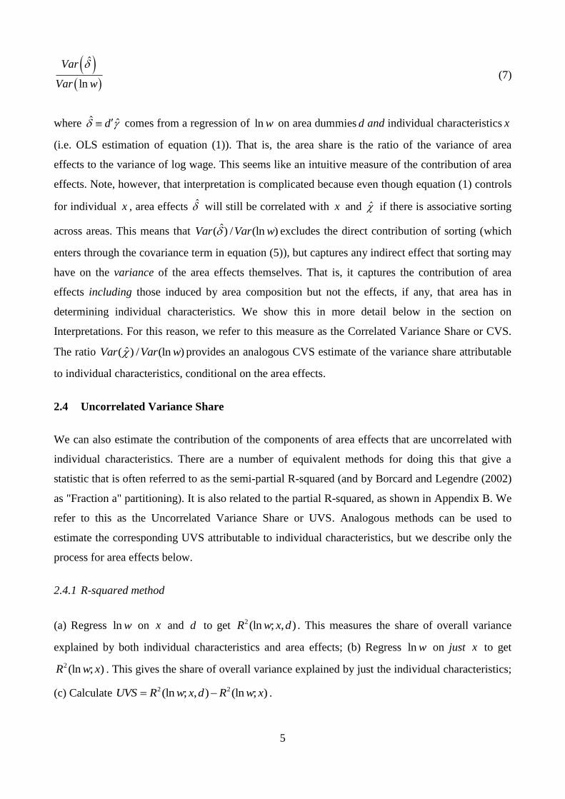
where ˆ ˆd comes from a regression of ln w on area dummies d and individual characteristics x

(i.e. OLS estimation of equation (1)). That is, the area share is the ratio of the variance of area

effects to the variance of log wage. This seems like an intuitive measure of the contribution of area

effects. Note, however, that interpretation is complicated because even though equation (1) controls

for individual x , area effects ̂ will still be correlated with x and ̂ if there is associative sorting

across areas. This means that ˆ( ) / (ln )Var Var w excludes the direct contribution of sorting (which

enters through the covariance term in equation (5)), but captures any indirect effect that sorting may

have on the variance of the area effects themselves. That is, it captures the contribution of area

effects including those induced by area composition but not the effects, if any, that area has in

determining individual characteristics. We show this in more detail below in the section on

Interpretations. For this reason, we refer to this measure as the Correlated Variance Share or CVS.

The ratio ˆ( ) / (ln )Var Var w provides an analogous CVS estimate of the variance share attributable

to individual characteristics, conditional on the area effects.

2.4 Uncorrelated Variance Share

We can also estimate the contribution of the components of area effects that are uncorrelated with

individual characteristics. There are a number of equivalent methods for doing this that give a

statistic that is often referred to as the semi-partial R-squared (and by Borcard and Legendre (2002)

as "Fraction a" partitioning). It is also related to the partial R-squared, as shown in Appendix B. We

refer to this as the Uncorrelated Variance Share or UVS. Analogous methods can be used to

estimate the corresponding UVS attributable to individual characteristics, but we describe only the

process for area effects below.

2.4.1 R-squared method

(a) Regress ln w on x and d to get 2(ln ; , )R w x d . This measures the share of overall variance

explained by both individual characteristics and area effects; (b) Regress ln w on just x to get

2 (ln ; )R w x . This gives the share of overall variance explained by just the individual characteristics;

(c) Calculate 2 2(ln ; , ) (ln ; )UVS R w x d R w x .

6

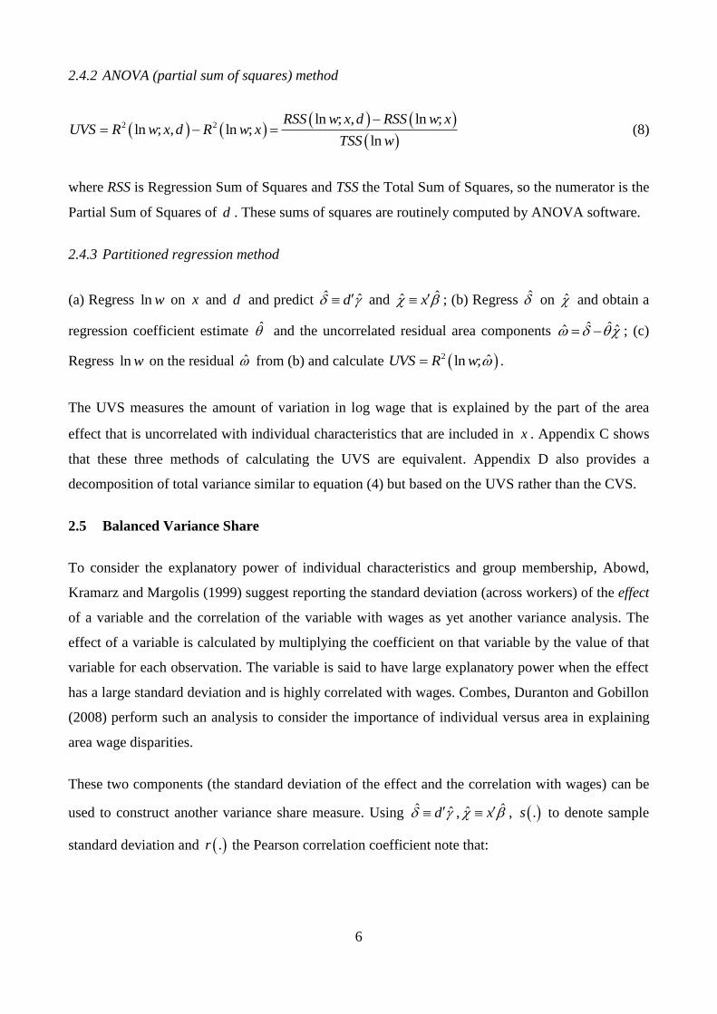
2.4.2 ANOVA (partial sum of squares) method

2 2

ln ; , ln ;ln ; , ln ;

ln

RSS w x d RSS w xUVS R w x d R w x

TSS w

(8)

where RSS is Regression Sum of Squares and TSS the Total Sum of Squares, so the numerator is the

Partial Sum of Squares of d . These sums of squares are routinely computed by ANOVA software.

2.4.3 Partitioned regression method

(a) Regress ln w on x and d and predict ˆ ˆd and ˆˆ x ; (b) Regress ̂ on ̂ and obtain a

regression coefficient estimate ̂ and the uncorrelated residual area components ˆ ˆˆ ˆ ; (c)

Regress ln w on the residual ̂ from (b) and calculate 2 ˆln ;UVS R w .

The UVS measures the amount of variation in log wage that is explained by the part of the area

effect that is uncorrelated with individual characteristics that are included in x . Appendix C shows

that these three methods of calculating the UVS are equivalent. Appendix D also provides a

decomposition of total variance similar to equation (4) but based on the UVS rather than the CVS.

2.5 Balanced Variance Share

To consider the explanatory power of individual characteristics and group membership, Abowd,

Kramarz and Margolis (1999) suggest reporting the standard deviation (across workers) of the effect

of a variable and the correlation of the variable with wages as yet another variance analysis. The

effect of a variable is calculated by multiplying the coefficient on that variable by the value of that

variable for each observation. The variable is said to have large explanatory power when the effect

has a large standard deviation and is highly correlated with wages. Combes, Duranton and Gobillon

(2008) perform such an analysis to consider the importance of individual versus area in explaining

area wage disparities.

These two components (the standard deviation of the effect and the correlation with wages) can be

used to construct another variance share measure. Using ˆ ˆd , ˆˆ x , .s to denote sample

standard deviation and .r the Pearson correlation coefficient note that:

7

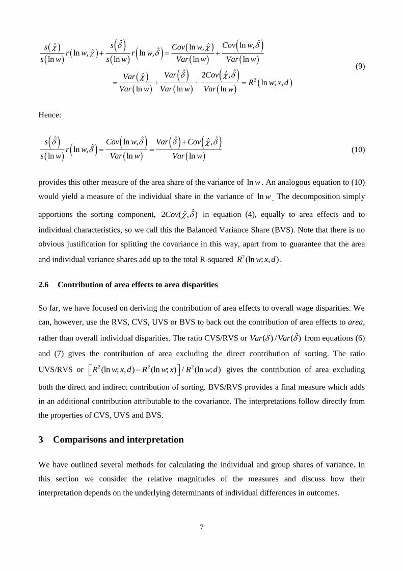
2

ˆ ˆln ,ˆ ˆln ,ˆˆln , ln ,ln ln ln ln

ˆ ˆˆ2 ,ˆln ; ,

ln ln ln

s Cov ws Cov wr w r w

s w s w Var w Var w

Var CovVarR w x d

Var w Var w Var w

(9)

Hence:

ˆ ˆ ˆ ˆˆln , ,ˆln ,

ln ln ln

s Cov w Var Covr w

s w Var w Var w

(10)

provides this other measure of the area share of the variance of ln w . An analogous equation to (10)

would yield a measure of the individual share in the variance of ln w . The decomposition simply

apportions the sorting component, ˆˆ2 ( , )Cov in equation (4), equally to area effects and to

individual characteristics, so we call this the Balanced Variance Share (BVS). Note that there is no

obvious justification for splitting the covariance in this way, apart from to guarantee that the area

and individual variance shares add up to the total R-squared 2(ln ; , )R w x d .

2.6 Contribution of area effects to area disparities

So far, we have focused on deriving the contribution of area effects to overall wage disparities. We

can, however, use the RVS, CVS, UVS or BVS to back out the contribution of area effects to area,

rather than overall individual disparities. The ratio CVS/RVS or ˆ( ) / ( )Var Var from equations (6)

and (7) gives the contribution of area excluding the direct contribution of sorting. The ratio

UVS/RVS or 2 2 2(ln ; , ) (ln ; ) / (ln ; )R w x d R w x R w d gives the contribution of area excluding

both the direct and indirect contribution of sorting. BVS/RVS provides a final measure which adds

in an additional contribution attributable to the covariance. The interpretations follow directly from

the properties of CVS, UVS and BVS.

3 Comparisons and interpretation

We have outlined several methods for calculating the individual and group shares of variance. In

this section we consider the relative magnitudes of the measures and discuss how their

interpretation depends on the underlying determinants of individual differences in outcomes.

8

3.1 Magnitudes

In Appendix C (equation A5), we show that 2 2ˆ ˆ ˆ(ln ; ) (1 2 ) ( ) / (ln )R w x Var Var w where ̂

is the coefficient from the regression of ˆ ˆd on ˆˆ x . An identical derivation gives:

2 2

2

ˆˆ ˆ(ln , ) (1 2 ) ( ) / (ln )

ˆ ˆˆ ˆ((1 ) ( ) 2 ( , )) / (ln )

RVS R w d Var Var w

Var Cov Var w

(11)

where ̂ is the coefficient from a regression of ˆˆ x on ˆ ˆd . Comparing to (7) it is

immediate that 2ˆ ˆ(1 2 )RVS CVS . Note that unless ˆ2 0 or ˆ( ) 0Var , RVS CVS .

That is, when individual characteristics are positively correlated with area effects (i.e. ˆ 0 ), RVS

is greater than CVS. In other words, the R-squared from a regression of ln w on area dummies will

attribute to area effects some of the contribution of individual characteristics. The same is true when

sorting is negative, and strong relative to the variance of area effects (i.e.

ˆ ˆˆ ˆ( , ) / ( ) 2Cov Var ). In the range ˆ2 0 , negative sorting tends to cancel out the

contribution of area effects when estimated using RVS. When ˆ 1 , negative sorting exactly

offsets area effects, so regression of ln w on area dummies would yield an RVS of zero, whereas

CVS would be positive.

Appendix C (equation A9) shows that the uncorrelated variance share is:

2ˆ ˆ ˆ

ln

Var VarUVS

Var w

(12)

where ̂ is the coefficient from the sample regression of ˆ ˆd on ˆˆ x . Comparing the

numerators in the UVS in (12) and CVS in (7):

2ˆ ˆ ˆ ˆ CVS Var Var Var UVS (13)

with equality if ̂ is uncorrelated with ̂ . Therefore the CVS gives an area share that is bigger than

that obtained by the UVS.

9

As we said before, the Balanced Variance Share, BVS adds ˆˆ ,Cov to the CVS. Hence, with

positive covariance between ̂ and ̂ , the BVS for area share is bigger than the CVS. From

equation (11) it is also clear that the RVS for area share is bigger than BVS, when there is positive

sorting (covariance). With negative sorting the BVS for area share is smaller than CVS, but it may

be larger or smaller than UVS or RVS. Finally, all methods give the same result if ̂ and ̂ are

uncorrelated. Naturally, these comparisons follow through to the decomposition of the variance of

ln w into the components attributed to area plus observable characteristics, versus unobservable

factors. For example, with positive sorting, adding up the BVS for area ( ˆ( )BVS ) and BVS for

individual characteristics ˆ( )BVS minimises the share of the variance attributed to unobservables

(i.e. it is the standard R-squared) and attributes as much as possible to ̂ and ̂ . At the other

extreme, adding ˆ( )UVS to ˆ( )UVS provides a more conservative estimate of the share

attributable to area and individual characteristics based on the orthogonal components of ̂ and ̂

alone, and so assigns a greater share of ln w to unknown components.

Given that all of the methods give a different answer when there is associative sorting of individuals

across groups it is natural to ask how we should interpret the different calculations and whether we

should prefer any specific method. This depends on the underlying factors determining individual

and area outcomes as we now show.

3.2 Interpretations

In order to gain some understanding of what contributes to each of these variance shares, it is

helpful to fully specify a system of linear equations which determine individual wages, area effects

and individual characteristics. Continuing to use d and x :

Individual wages: ln w (1)

Area effects: (14)

Individual characteristics: (15)

The equation for individual wages is identical to that used earlier in Section 2. As shown in

equation (14) we allow area effects to be determined by average area composition (where the mean

of is taken across individuals, within areas) and by exogenous variation (e.g. climate).

10

Equation (15) allows individual characteristics to be determined by area and by exogenous

individual specific variation v (e.g. innate ability). Specifying equation (15) in terms of rather

than x simplifies later notation.

Averaging (15) at the area level gives area-mean individual characteristics , and it is

correlation between these and area effects that biases estimations of the relative contributions of

individual and area effects. Part of this correlation arises because of the interdependency between

and explicit in (14) and (15) when 0 and/or 0 . However, there is an additional

correlation, present even when 0 and 0 if , 0Cov .That is, if exogenous area effects

( ) and area-mean exogenous individual characteristics ( )v are correlated through sorting

processes that are otherwise unrelated to wages (e.g. if higher skill people prefer warmer climates).

Note that all this assumes that the underlying sources of variance across areas are the exogenous

additive components , and rules out multiple equilibria that arise in theoretical models. Even

in this very restricted world, it turns out to be difficult to provide firm statements about the share of

area effects or whether RVS, BVS, CVS or UVS provides the most appropriate empirical measure.

In the Appendix E, we show that equations (1), (14) and (15) can be used to get expressions for the

variance of area effects, mean individual characteristics and their covariance in terms of the

underlying structural errors and parameters:

2 2( ) ( ( ) ( ) 2 ( , ) / (1 )Var Var v Var Cov v (16)

2 2( ) ( ) ( ) 2 ( , ) / (1 )Var Var v Var Cov v (17)

2( , ) ( ) ( ) (1 ) , / (1 )Cov Var Var v Cov v (18)

If area affects individual characteristics ( 0 ) equations (17) and (18) show that the exogenous

component of area effects ( ) enters into Var and ,Cov . Similarly if area composition

determines area effects ( 0 ), equations (16) and (18) show that the exogenous component of

individual characteristics ( ) enters into Var and ,Cov . (Positive) sorting,

, 0Cov increases Var if area effects are increasing in ( 0 ) and increases Var

if individual characteristics are increasing in ( 0) . Positive sorting also increases ,Cov ,

11

with the increase greater if both 0 and 0 . These results regarding carry through to the

distribution of individual characteristics because , ,Cov Cov and

Var Var Var , where represents all the within-area individual components of

wages. In short, Var , Var and ,Cov , which are observable, cannot be attributed to one

or other of the potentially unobservable exogenous components , that are the underlying

sources of variance across areas in the simple system represented in equations (1), (14) and (15).

Turning to the four variance shares, it’s useful to repeat the formulas:5

2 ˆ ˆˆ ˆ(1 ) ( ) 2 ( , )

ln ln

Var CovRVS

Var w Var w

,

ˆ ˆˆ( ) ( , )

ln ln

Var CovBVS

Var w Var w

ˆ

ln

VarCVS

Var w

,

2ˆ ˆ ˆ

ln

Var VarUVS

Var w

It can be seen that equations (16) - (18) can, in principle, be used to express the four variance shares

in terms of the underlying structural components. It should be clear, however, that even in this very

basic linear world there is no simple relationship between these variance shares and the underlying

structural components. Which variance share is most appropriate depends on a complex interplay

between: (a) the underlying structural component in which we are interested; (b) the magnitudes

and signs of the coefficients determining area effects and individual characteristics; and (c) sorting.

One simple case occurs when composition does not cause area effects ( 0 ), in which case CVS

gives the variance share of the area shocks . Correspondingly, when area does not cause changes

in individual characteristics ( 0 ), ˆ lnVar Var w gives the share of individual

characteristics in log wages. Note too that when 0 , ,Cov provides an unbiased

estimate of the degree of sorting but otherwise combines the covariance caused by sorting and by

5 In these expressions, remember that ̂ is the coefficient from the regression of ̂ on ̂ (i.e. ˆ ˆˆ , / ( )Cov Var

not the ‘structural’ coefficient in equation (15)) and ̂ is the coefficient from the regression of ̂ on ̂ (i.e.

ˆˆ ˆ, / ( )Cov Var not the ‘structural’ coefficient in equation (14)). We ignore this complication in the text, but

note that the problems of linking variance shares to structural components persist even in the unlikely case that sample

estimates equal their population values.

12

the causal influence of area on characteristics (and vice-versa). In all other contexts, pinning down

the contribution of specific sources of area-level variations is not possible, but as discussed above

RVS, BVS, CVS and UVS can at least be used to provide a bounding exercise to guide us as to the

likely contributions.

4 Application: wage disparities in Britain

In this section we use the four variance shares to look at the contribution of individual and area

effects to wage variation in Britain. We improve on existing UK work on regional inequalities

(Duranton and Monastiriotis (2002), Taylor (2006) and Dickey (2007)) by working with functional

labour market areas (rather than administrative boundaries) at a smaller spatial scale and by using

panel data to control for unobserved individual characteristics. Outside of the UK, a number of

existing studies have already used individual data to study spatial sorting and agglomeration

economies. See, for example, Mion and Natticchioni (2009), Dalmazzo and Blasio (2007) and

Combes, Duranton and Gobillon (2008). This paper is most closely related to the last of these but

pays more attention to the issue of the share of disparities attributable to area effects using the

insights developed above.

We use data for 1998-2008 from the Annual Survey of Hours and Earnings (ASHE) and its

predecessor the New Earnings Survey (NES). NES/ASHE are constructed by the Office of National

Statistics (ONS) based on a 1% sample of employees on the Inland Revenue PAYE register for

February and April. The sample is of employees whose National Insurance numbers end with two

specific digits and workers are observed for multiple years (up to 11 years given the time span of

our sample). The sample is replenished as workers leave the PAYE system (e.g. to retirement) and

new workers enter it (e.g. from school). NES/ASHE include information on occupation, industry,

whether the job is private or public sector, the workers age and gender and detailed information on

earnings. We use basic hourly earnings as our measure of wages. NES/ASHE do not provide data

on education but information on occupation works as a good proxy for our purposes. NES/ASHE

provide national sample weights but as we are focused on sub-national (TTWA) data we do not use

them in the results we report below.

ASHE provides information on individuals including their home and work postcodes, while the

NES only reports work postcodes. We use the National Statistics Postcode Directory (NSPD) to

assign workers to Travel to Work Areas (TTWA) using their work postcode, allowing us to use the

whole NES/ASHE sample over our study period. Given the way TTWA are constructed (so that

13

80% of the resident population also work within the area) the work TTWA will also be the home

TTWA for the majority of workers. To ensure reasonable sample sizes, our analysis divides Britain

into 157 “labour market areas” of which 79 are single “urban” TTWA and 78 are “rural areas”

created by combining TTWAs.6

We derive estimates of RVS, CVS, UVS and BVS, from regression analysis of individual wages,

based on equation (1) above, but adapted to include individual fixed effects and time dummies to

take advantage of the panel dimension of our data:

' 'ln ijt i t it jt ijtw x d (19)

where j indexes areas, i are individual fixed effects, the t are time dummies, itx is a vector of

time varying individual characteristics, and everything else is as in equation (1). captures the

impact of individual characteristics controlling for area . Likewise, captures the impact of area

controlling for both time invariant unobserved individual characteristics ( i ) and time varying

observed individual characteristics ( itx ). These parameter estimates, allow us to obtain estimates of

ˆ d and ˆˆ x from which we can calculate RVS, CVS, UVS and BVS.

Including individual fixed effects means that identification of the area fixed effects comes from

movers across areas. As usual, we cannot rule out the possibility that shocks to it

are correlated

with the decision to move so the area effect estimates need to be interpreted with some caution. In

the absence of random allocation (or a policy change that as good as randomly assigns people)

tracking individuals and observing the change in wages experienced when they move between areas

is the best we can do to identify causal area effects.7 Estimating the area effects from movers means

we need to assume fixed-across-time area effects.8 We shall show, however, that dropping

individual fixed effects and controlling for observables only provides area effects estimates that are

very stable over time. Given this, and as individual unobserved characteristics are important for

6 We reached this classification in three steps: a) we identified the primary urban TTWAs as TTWA centred around, or

intersecting urban-footprints with populations of 100,000 plus; b) we identified TTWA with an annual average

NES/ASHE sample size greater than 200 as stand-alone non-primary-urban TTWA (e.g. Inverness); and c) we grouped

remaining TTWA (with sample sizes below 200) into contiguous units (e.g. North Scotland). 7 Note, that we track individuals in the panel for up to 10 years, so the wage changes we observe for individuals moving

between areas are not just the one-off changes when the move occurs, but include longer-run changes (e.g. due to

differences in wage growth rates between areas). 8 Theoretically, we could still allow for such year on year changes in place specific effects, but identifying them

requires movers in and out of all areas in every year which turns out to be too demanding given our sample sizes.

14

explaining wages, our preferred specification incorporates individual effects but assumes area

effects are fixed across time. Some basic descriptive statistics are provided in Appendix F.

We start by estimating equation (19) with an increasing set of control variables to show how

allowing for sorting across areas affects the magnitude of estimated area effects. To summarise the

distribution of effects we first report the percentage change in wages when moving between

different parts of the area effects distribution: the minimum to maximum and to mean, mean to

maximum, the 10th

to the 90th

percentile and the 25th

to the 75th

percentile. Table 1 reports results

based on several different specifications. The first row reports results from equation (19) when only

including time dummies (which gives the upper bound estimates of area effects). The second row

reports results when the observable variables are a set of age dummies, a gender dummy and a set

of 1 digit occupation dummies. The third row uses a set of age dummies, a gender dummy, two

digit occupation dummies, industrial dummies (three digit SIC) and dummies for public sector

workers, part time workers and whether the worker is part of a collective agreement. Results using

individual fixed effects are reported in rows four and five. In row four, we simply include year

dummies and individual effects. Row five uses individual effects, year dummies, age dummies and

one digit occupation dummies.

Table 1: Distribution of area effects ( ̂ )

Controls: min-max

min-

mean

mean-

max p90-p10 p75-p25

Year dummies 61.7% 18.2% 36.8% 22.0% 10.6%

+ age, gender, occ-1 36.6% 9.0% 25.4% 12.7% 6.4%

+age, gender, occ-2, sic-3, public, union, part-

time 29.0% 6.5% 21.0% 9.7% 4.2%

Individual fixed effects and year dummies 20.3% 7.6% 11.8% 8.9% 4.4%

+ age, occ1 17.3% 5.9% 10.8% 7.3% 3.8%

Notes: Authors own calculations based on NES/ASHE. Specifications are described in detail in the text (occ-

1, occ-2 signify one and two digit occupation; sic-3 signifies three digit industry code). Results for 157 areas.

Based on 1,511,163 observations (305, 752 individuals)

If we ignore the role of sorting (i.e. do not control for i and itx ) then the differences in area

average wages look quite large. Moving from the worst to the best area, average wages increase by

just over 60%; from the minimum to the mean by a little under 20%; and from the mean to the

maximum by just over 35%. Of course the minimum and maximum represent extremes of the

distribution. The move from the 10th

to the 90th

percentile sees average wages increase by 22%,

from the 25th

to 75th

percentile by just over 10%. Introducing a limited set of observable

characteristics (row 2) to control for sorting substantially reduces estimated area differences. A

15

larger set of individual characteristics (row 3) reduces the estimated differences further as does

allowing for individual fixed effects, with or without additional observable characteristics (rows 4

and 5). Interpreting observed area differences as area effects considerably overstates the impact on

wages that occurs as individuals move from bad to good areas. Specifically, across the comparisons

we report, ignoring the role of sorting overstates area effects by a factor of three.

As discussed above, the contribution of area effects to overall (and area) wage disparities depends

not only on the size of specific effects but also on the overall distribution of area effects and on the

distribution of individuals across those areas. We suggested four alternative variance

decompositions for measuring this contribution. Table 2 reports results for the contribution of area

differences to overall and area wage disparities using these four measures. We calculate them from

regression specifications using the same individual characteristics as in Table 1. For comparison,

the second panel of the table reports the contribution of the individual characteristics using the

different measures while the third panel reports the contribution of area effects to area disparities.

Table 2: Variance decomposition

Year

dummies

only (RVS)

+ age,

gender,

occ-1

+ age,

gender,

occ-2, sic-3,

public,

union, pt

Individual

fixed effects

and year

dummies + age, occ-1

(1) (2) (3) (4) (5)

Area variance share

ˆ( )BVS 6.0% 3.2% 2.4% 1.1% 0.9%

ˆ( )CVS 6.0% 2.8% 2.0% 0.7% 0.6%

ˆ( )UVS 6.0% 2.7% 1.3% 0.1% 0.1%

Individual variance share

ˆ( )BVS 57.7% 75.9% 86.8% 88.3%

ˆ( )CVS 57.4% 75.5% 86.4% 87.9%

ˆ( )UVS 54.0% 73.0% 83.6% 84.9%

Area share of area disparities

ˆ( ) /BVS RVS 53.2% 40.4% 18.3% 15.9%

ˆ( ) /CVS RVS 47.5% 34.1% 12.6% 10.4%

ˆ( ) /UVS RVS 45.8% 22.3% 1.3% 1.1%

Notes: Authors own calculations based on NES/ASHE. Specifications are described in detail in the text

(occ-1, occ-2 signify one and two digit occupation; sic-3 signifies three digit industry code; pt signifies part-

time). Based on 1,511,163 observations (305, 752 individuals).

16

The top panel of Table 2, column 1 shows that even if we ignore the effects of sorting, and simply

consider raw area differences in mean log wages, areas only explain 6% of the overall variation in

wages across individuals (remember that in the absence of controls for any individual

characteristics the variance share of area effects is the same whichever way it is calculated). Moving

across the columns in Table 2, panel 1, we progressively add controls for individual characteristics,

culminating in a specification with individual fixed effects in columns 4 and 5. Looking down rows

within the top panel shows how the variance share changes according to the way we estimate it –

Balanced Variance Share (BVS), Correlated Variance Share (CVS) and Uncorrelated Variance

Share (UVS). As discussed in Section 3.1, the Correlated Variance Share provides an upper bound

to the combined contribution of exogenous area effects plus those induced by area composition (i.e.

the area mean individual characteristics). The Uncorrelated Variance Share provides a lower bound

to the contribution of exogenous area effects alone. The Balanced Variance Share could be larger or

smaller than the Correlated Variance Share, depending on whether there is positive or negative

assortative matching of individuals to areas. It is evident from the fact that BVS> CVS > UVS in

Table 2, that we have positive sorting across areas. On any of these measures, the contribution of

area effects is around 3% or less when controlling for basic observable characteristics (columns 2

and 3) and around 1% or less when controlling for unobservable individual characteristics (columns

4 and 5). In short, the most striking finding from Table 2 is that area effects only play a small role

in explaining overall individual wage disparities.

We have shown (in Section 3) that it is not , in general, possible to determine from these variance

shares the exact contribution of sorting, versus the influence of area composition on area effects,

versus the influence of area effects on area composition. However, comparison of the CVS(̂ ) and

UVS( ̂ ) measures is partly revealing. Looking at the gap between the UVS and CVS in our

preferred specifications with individual fixed effects in columns 4 and 5 of panel 1 suggests that

area effects arising from area composition account for over half of everything that can be attributed

to area effects. To see this, note that CVS( ̂ ) – UVS( ̂ ) is more than 50% of either CVS( ̂ ) (or

even BVS( ̂ )), in columns 4 and 5. Even so, this is still a trivial share of the overall individual

disparity in wages - roughly 0.5% in our preferred specification (CVS( ̂ ) – UVS( ̂ ) in column 5.

In contrast to these results on area effects, the contribution of individual characteristics shown in the

second panel of Table 2 is very large. Age, gender and occupation variables alone account for 54-

58% of the individual variation in wages. Adding in individual fixed effects drives this share up to

between 85% and 88% in the last column, implying that the contribution of individual

17

characteristics is between 100 times (comparing BVS) and 850 times (comparing UVS) bigger than

that of area effects. Comparison of CVS( ̂ ) and UVS( ̂ ) implies that area effects also contribute

very little to the variance of individual effects on wages.

The final panel of the table shows that area effects as defined here play a somewhat more important

role in explaining the area disparities captured by the simple between-area variance share (the RVS

in Table 2). When controlling for basic characteristics, sorting accounts for a little over half of the

observed area disparities leaving area effects to account for around 48%. Once controlling for

individual fixed effects the upper bound estimate of the contribution of area effects to area

disparities is considerably smaller at a little over 10% with the lower bound estimate around 1%.

Even so, the dominant contribution to area disparities (one minus the share reported in the final

panel of Table 2) must come from individual characteristics, and the way these are distributed

across areas.

Table 3: Area effects: Results by year

RVS BVS CVS UVS

Pooled 6.0% 2.4% 2.0% 1.3%

1998 6.2% 2.3% 1.9% 0.8%

1999 6.0% 2.2% 1.9% 0.8%

2000 6.0% 2.2% 1.9% 0.8%

2001 6.3% 2.3% 2.0% 0.9%

2002 6.6% 2.7% 2.3% 1.2%

2003 6.6% 2.7% 2.3% 1.3%

2004 6.6% 2.7% 2.3% 1.3%

2005 6.5% 2.5% 2.1% 1.2%

2006 6.2% 2.4% 2.1% 1.2%

2007 6.8% 2.5% 2.1% 1.1%

2008 6.7% 2.5% 2.1% 1.1%

Notes: Based on 1,511,163 observations (305, 752 individuals). Contribution for pooled lower than

average of years because pooled regressions impose time invariant area effects and coefficients on

individual characteristics. The pooled estimate of Column 1 controls for year effects. All estimates in

Columns 2 and 3 control for age, gender, 2-digit occupation, 3-digit SIC, public sector, union and

part-time.

Table 2 has shown these decompositions based on pooling all years in our dataset. The results in

Table 3 investigate the stability of the contribution of area effects over time, and shows that this

contribution has been stable. For each year, the table reports the contribution of the four area

variance shares controlling for the fullest possible set of individual characteristics. For comparison,

the first row reports results when pooling across years (taken from Table 2). Repeating other results

from Table 2 by year give figures that are similarly stable across years. As discussed above, it is

18

this stability of area effects across time, combined with the importance of individual effects which

leads us to view the individual fixed effects constant-across-time area effects specifications reported

in the final two columns of table 2 as our preferred specification.

5 Conclusions

This paper has reviewed a number of ways to decompose variance in wages into the contribution

from individual and area specific effects. The paper collates the methods present in the literature,

discusses how different variance decompositions are related to each other and how they should be

interpreted, and finally, highlights that a clear-cut division of variation into components is strictly

speaking impossible, and that whatever method a researcher chooses, assumptions and caveats will

remain.

In particular, we have discussed decompositions that we named Raw Variance Share (RVS),

Balanced Variance Share (BVS), Correlated Variance Share (CVS) and Uncorrelated Variance

Share (UVS). We have shown why disentangling the contribution of area effects to wage

distribution is complex, and why an approach based on bounds such as RVS, BVS, CVS and UVS

can only provide guidance to the relative importance of area effects.

The RVS is the simple between-area share of the total variance and provides an overall upper bound

for the contribution of area effect on total wage variation. It counts the average differences in

worker characteristics across areas as part of the area effect. For Britain, this measure has

persistently accounted for roughly 6% of the overall wage variation for over a decade. The CVS

excludes the direct contribution of sorting, but captures the effect that sorting may have on the

variance of the area effect. We interpreted the CVS as an upper bound to the combined contribution

of exogenous area effects plus interactions-based spillovers that are linked to the mean

characteristics of individuals in each area. CVS in Britain has been around 2%, but less than 1% if

individual fixed unobservable effects are controlled for. The alternative BVS decomposition that

has appeared in previous work (e.g. Abowd, Kramarz, Margolis 1999, Combes Duranton and

Gobillon 2008) yields a slightly higher estimate of the contribution of area effects in our setting,

because there is positive assortative matching of individuals to areas (i.e. individual wage effects

are correlated with area wage effects). However, in general, this measure is quite hard to interpret,

since it mixes up the variance attributable to areas with the covariance between area effects and

area-mean individual effects. We argue that CVS is a more natural indicator. Finally, compared to

CVS, UVS further excludes the effects that sorting may have on the variation of the area effects,

19

and such provides a lower bound to the contribution of exogenous area effects. With this measure,

the area effects explain 1.5% of wage variation in Britain. If individual fixed effects are included,

the effect shrinks to less than 0.1%, and this should be considered as the lower bound of the effect

of area on variation of wages.

Whichever estimate we use, our general finding is that most of the observed regional inequality in

average wage in Britain is explained by ‘sorting’ or ‘people’ rather than ‘places’. Our preferred

estimates, which include the individual fixed effects, suggest that the contribution of individual

characteristics to variation in wages is between 100 to 850 times larger than the contribution of area

effects.

6 References

Abowd, John, Francis Kramarz, and David Margolis (1999). “High wage workers and high wage

firms.” Econometrica 67(2), 251-334.

Abowd, John., Robert Creecy, and Francis Kramarz (2002), Computing Person and Firm Effects

Using Linked Longitudinal Employer-Employee Data, Cornell University Working Paper

Fisher, Ronald A. (1933) in a letter to L.Hogben 25 February. Printed in Natural Selection,

Heredity, and Eugenics, p.218, J.H.Bennett, Oxford: Clarendon Press, 1983 quoted on

http://www.economics.soton.ac.uk/staff/aldrich/fisherguide/quotations.htm (accessed February

2012)

Borcard, Daniel and Legendre, Pierre (2002). “All-scale spatial analysis of ecological data by

means of principal coordinates of neighbour matrices.” Ecological Modelling, 153(1-2), 51-68.

Combes, Pierre Philppe, Gilles Duranton and Laurent Gobillon. (2008). “Spatial wage disparities:

Sorting matters!” Journal of Urban Economics, 63(2), 723-742.

Dalmazzo, Alberto and Guido de Blassio (2007). “Social Returns to Education in Italian Local

Labour Markets,” The Annals of Regional Science, 41(1), 51-69.

Dickey, Heather (2007). Regional Earnings Inequality In Great Britain: Evidence From Quantile

Regressions," Journal of Regional Science, 47(4), 775-806.

Duranton, Gilles. and Vassilis. Monastiriotis (2002). “Mind the Gaps: The Evolution of Regional

Earnings Inequalities in the U.K., 1982-1997,” Journal of Regional Science, 42(2), 219-256.

Gibbons, Robert. S. and Lawrence. Katz (1992). “Does Unmeasured Ability Explain Inter-Industry

Wage Differences?” Review of Economic Studies, 59, 515-35.

Goldstein, Harvey. (2010) Multilevel Statistical Models, 4th edition, Wiley-Blackwell

20

Kramarz, Francis, Stephen Machin, and Amine Ouazad, (2009) “What Makes a Test Score? The

Respective Contributions of Pupils, Schools and Peers in Achievement in English Primary

Education” London School of Economics, Centre for Economics of Education CEEDP0102:

Krueger, Alan and Lawrence. H. Summers (1988). “Efficiency Wages and the Inter-industry Wage

Structure,” Econometrica, 56(2), 259-93.

Mion, Giordano and Paolo Naticchioni (2009). “The spatial sorting and matching of skills and

firms,” Canadian Journal of Economics, 42(1), 28-55.

Office for National Statistics, Annual Survey of Hours and Earnings, 1997-2009: Secure Data

Service Access [computer file]. Colchester, Essex: UK Data Archive [distributor], March 2011. SN:

6689.

Ouazad, Amine (2008) A2REG: Stata module to estimate models with two fixed effects," Statistical

Software Components. S456942, Boston College Department of Economics.

Taylor, Karl. (2006). “UK Wage Inequality: An Industry and Regional Perspective,” Labour:

Review of Labour Economics and Industrial Relations, 20(1), 91-124.

Appendix A: Extension to individual and area fixed effects

All the methods can be generalised to allow for multiple effects f f fh , where and are

particular cases of f , such that equation (2) becomes:9

ln f f f

f f

w h (A1)

Then the raw variance share for the contribution of any one of these effects f is:

2( )

(ln , )(ln )

f

f

VarR w h

Var w

where f f fh , f is the coefficient vector and 2 (ln , )fR w h the R-squared from the regression

of ln w on dummies (or other variables) fh , with no control for ~ f , where the notation ~ f means

the set of all effects not including f . The variance decomposition of ln wages is:

9 The stata routine a2reg for two way fixed effects (Ouazad 2008), based on Abowd, Creecy and Kramarz (2002), is

useful for practical implementation in applications including two groups of effects (for example individual and area

effects). See http://courses.cit.cornell.edu/jma7/abowd-creecy-kramarz-computation.pdf.

21

ˆ ˆ ˆ, ˆ1

ln ln ln

f f g

f f g g f

Var Cov Var

Var w Var w Var w

(A2)

Where ˆ ˆf f fh , ˆ

f are the coefficients from OLS estimation of (A11) and the correlated

variance share =

ˆ

ln

fVar

Var w

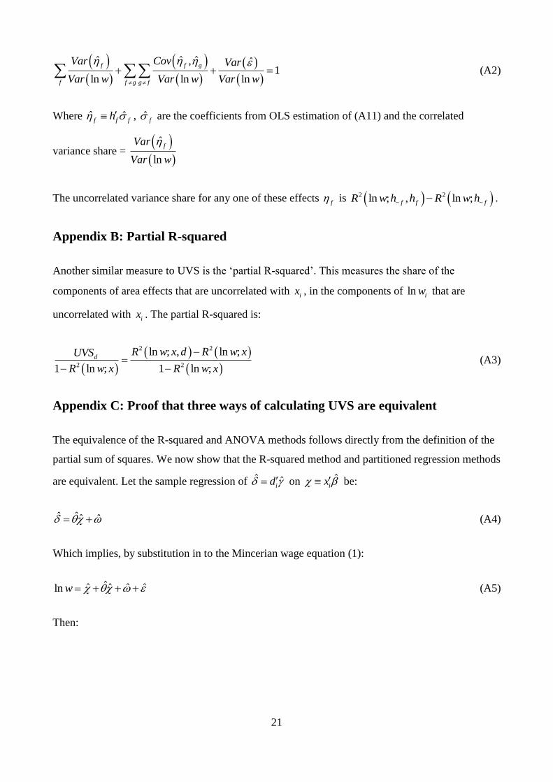
The uncorrelated variance share for any one of these effects f is 2 2

~ ~ln ; , ln ;f f fR w h h R w h .

Appendix B: Partial R-squared

Another similar measure to UVS is the ‘partial R-squared’. This measures the share of the

components of area effects that are uncorrelated with ix , in the components of ln iw that are

uncorrelated with ix . The partial R-squared is:

2 2

2 2

ln ; , ln ;

1 ln ; 1 ln ;

dR w x d R w xUVS

R w x R w x

(A3)

Appendix C: Proof that three ways of calculating UVS are equivalent

The equivalence of the R-squared and ANOVA methods follows directly from the definition of the

partial sum of squares. We now show that the R-squared method and partitioned regression methods

are equivalent. Let the sample regression of ˆ ˆid on ˆ

ix be:

ˆ ˆˆ ˆ (A4)

Which implies, by substitution in to the Mincerian wage equation (1):

ˆˆ ˆ ˆ ˆln w (A5)

Then:

22

2

ˆ ˆˆ2 ,ˆln ; ,

ln ln ln

ˆ ˆˆ ˆ2

ln ln ln

Var CovVarR w x d

Var w Var w Var w

VarVar Var

Var w Var w Var w

(A6)

where the first line follows from the full variance decomposition (4) and the second line follows

from equation A4. Now, from equation (A4):

2

2

ˆ ˆ ˆˆ1 ˆ1 2ln ;

ln ln

Var VarR w x

Var w Var w

(A7)

So from (A5) and (A6) we have:

2

2 2

ˆ ˆ ˆln ; , ln ;

ln

Var VarR w x d R w x

Var w

(A8)

Now in the Partitioned regression method:

2

ˆˆln ;

ln

VarR w

Var w

(A9)

Where the numerator is:

2

2

2

ˆ ˆ ˆ ˆˆ ˆ ˆ2 ,

ˆ ˆ ˆˆ ˆ2

ˆ ˆ ˆ

Var Var Var Cov

Var Var Var

Var Var

(A10)

Hence from (A7)-(A9) the uncorrelated variance share is:

2

2 2 2

ˆ ˆ ˆˆln ; ln ; , ln ;

ln

Var VarR w R w x d R w x

Var w

(A11)

and so the R-squared and partitioned regression methods are equivalent.

23

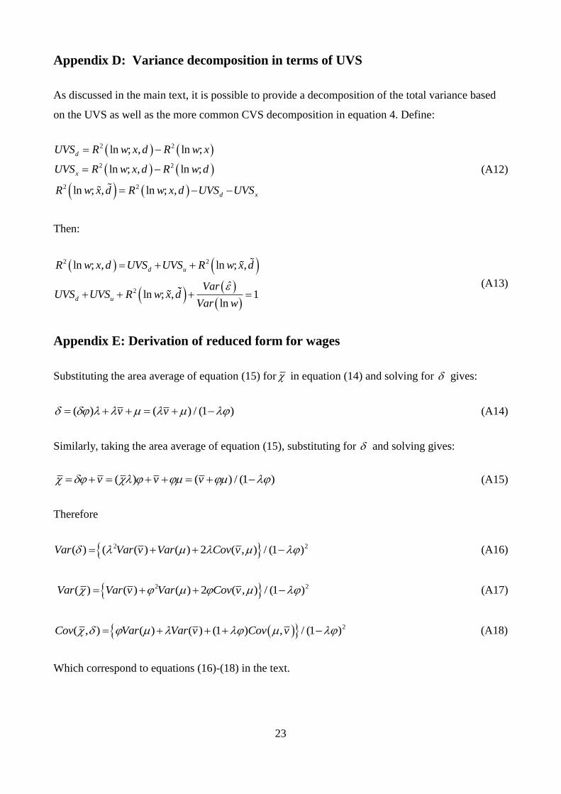
Appendix D: Variance decomposition in terms of UVS

As discussed in the main text, it is possible to provide a decomposition of the total variance based

on the UVS as well as the more common CVS decomposition in equation 4. Define:

2 2

2 2

2 2

ln ; , ln ;

ln ; , ln ;

ln ; , ln ; ,

d

x

d x

UVS R w x d R w x

UVS R w x d R w d

R w x d R w x d UVS UVS

(A12)

Then:

2 2

2

ln ; , ln ; ,

ˆln ; , 1

ln

d u

d u

R w x d UVS UVS R w x d

VarUVS UVS R w x d

Var w

(A13)

Appendix E: Derivation of reduced form for wages

Substituting the area average of equation (15) for in equation (14) and solving for gives:

( ) ( ) / (1 )v v (A14)

Similarly, taking the area average of equation (15), substituting for and solving gives:

( ) ( ) / (1 )v v v (A15)

Therefore

2 2( ) ( ( ) ( ) 2 ( , ) / (1 )Var Var v Var Cov v (A16)

2 2( ) ( ) ( ) 2 ( , ) / (1 )Var Var v Var Cov v (A17)

2( , ) ( ) ( ) (1 ) , / (1 )Cov Var Var v Cov v (A18)

Which correspond to equations (16)-(18) in the text.

24

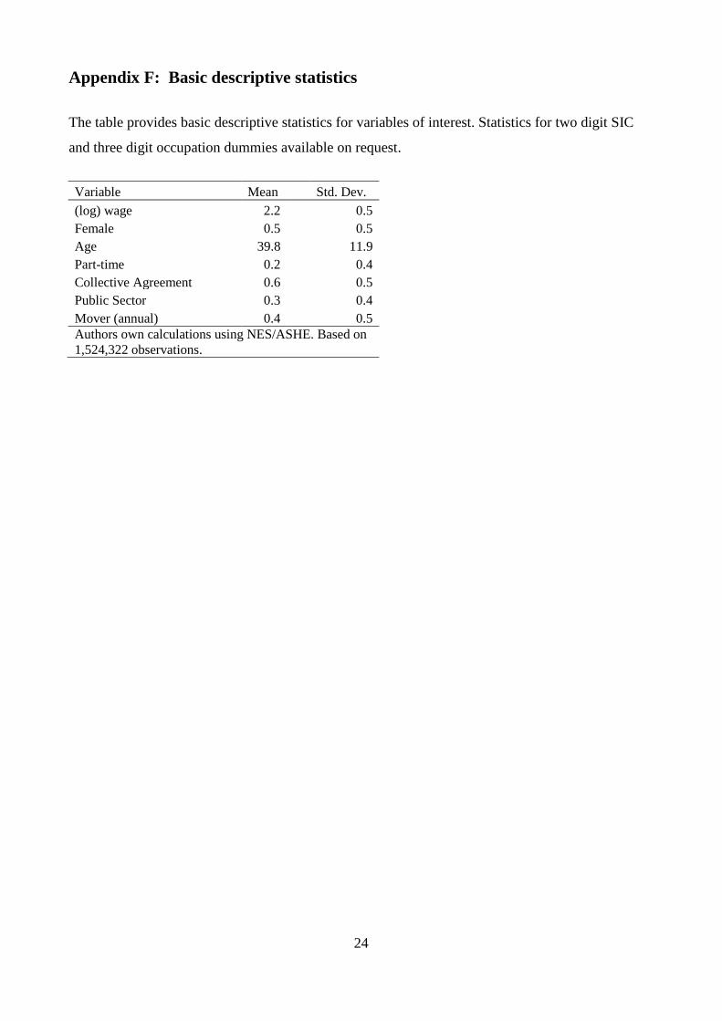
Appendix F: Basic descriptive statistics

The table provides basic descriptive statistics for variables of interest. Statistics for two digit SIC

and three digit occupation dummies available on request.

Variable Mean Std. Dev.

(log) wage 2.2 0.5

Female 0.5 0.5

Age 39.8 11.9

Part-time 0.2 0.4

Collective Agreement 0.6 0.5

Public Sector 0.3 0.4

Mover (annual) 0.4 0.5

Authors own calculations using NES/ASHE. Based on

1,524,322 observations.