1 a perceptually inspired variational framework for...
TRANSCRIPT
1
A Perceptually Inspired Variational Framework
for Color Enhancement
Rodrigo Palma, Edoardo Provenzi, Marcelo Bertalmıo and Vicent Caselles
Abstract
Basic phenomenology of human color vision has been widely taken as an inspiration to devise
explicit color correction algorithms. The behavior of these models in terms of significative image features
(such as, e.g., contrast and dispersion) can be difficult to characterize. To cope with this, we propose to
use a variational formulation of color contrast enhancement that is inspired by the basic phenomenology
of color perception. In particular, we devise a set of basic requirements to be fulfilled by an energy to be
considered as ‘perceptually inspired’, showing that there is an explicit class of functionals satisfying all
of them. We single out three explicit functionals that we consider of basic interest, showing similarities
and differences with existing models. The minima of such functionals is computed using a gradient
descent approach. We also present a general methodology to reduce the computational cost of the
algorithms under analysis from O(N2) to O(N log N), being N the number of input pixels.
Index Terms
Perceptual color enhancement, variational principles, gradient descent approach.
I. INTRODUCTION
Human vision is a process of great complexity that involves many features as, e.g., shape
and pattern recognition, motion analysis and color perception. An essential literature about
Rodrigo Palma is with Department of Electrical Engineering, Universidad de Chile, Avenida Tupper 2007, Casilla 412-
3, Santiago, Chile. E-mail: [email protected]. Tel. : +56 2 978 4207. Fax. +56 2 695 3881. Edoardo Provenzi is
with Dipartimento di Tecnologia dell’Informazione, Universita di Milano, Via Bramante 65, 26013, Crema (CR), Italy. E-
mail: [email protected]. Tel. +39 0373 898089. Fax. +39 0373 898010. Marcelo Bertalmıo and Vicent Caselles are
with Departament de Tecnologia, Universitat Pompeu Fabra, Pg. de Circumvallacio 8, 08003 Barcelona, Spain. E-mail:
[email protected], Tel. +34 93 542 25 69, Fax. +34 93 542 25 17; E-mail: [email protected], Tel. +34 93
542 24 21, Fax. +34 93 542 25 17.
2
neurophysiological aspects of human vision can be found in the books [1]–[7].
In this paper we will focus on color perception. This process begins with light capture by
the three different types of cone pigments inside the retina. They have different absorption
characteristics, with peak absorptions in the red, green and blue regions of the optical spectrum.
The existence of three types of cones provides a physiological basis for the trichromatic theory of
color vision. When a light stimulus activates a cone, a photochemical transition occurs, producing
a nerve impulse. Experimental evidence [7] show that the propagation of nerve impulses reach
the brain, which analyzes and interprets the information carried by the impulses. The part of
the brain devoted to color perception is the so-called V4 zone of the occipital cortex. Neither
retina photochemistry nor nerve impulses propagation are well understood, hence a deterministic
characterization of the visual process is still unavailable. For this reason, the majority of color
perception models follow a descriptive approach, trying to simulate macroscopic characteristics
of color vision, rather than reproduce neurophysiological activity.
The first modern contribution in such a field has been provided by the famous Retinex theory
of Land and McCann [8]. They started devising a series of innovative experiments about color
perception using unrealistic pictures called ‘Mondrians’ [9], [10]. The abstract character of the
images minimized the action of high level faculties of the Human Visual System (HVS) such
as memory learning, judgement and recognition, thus making possible the reproducibility of the
experiments [11]. They then found a formal computation able to reproduce experimental data,
providing the first Retinex model of color vision [8]. After that, a whole category of perceptually
inspired computational algorithms has been developed with different aims: reproduction of color
sensation, color stabilization, enhancement of color images, etc. [12]. A common characteristic
of these works is that HVS features are taken as inspiration to devise the explicit equations of
perceptually based algorithms.
In this paper, rather than dealing directly with explicit algorithms, we are interested in the
analysis of the interplay between color perception and variational image processing. The reason
is that variational techniques have proven to be a powerful instrument to both understanding
and solving image processing problems. Variational principles are based on energy functionals,
whose selection depends on the particular problem under examination. The image for which the
functional reaches a minimum is the solution to the particular image processing task at hand.
Since our aim is performing a perceptually inspired color correction, we are interested in the
3
analysis of energy functionals complying with the basic features of color perception. So, we
will provide a translation of basic macroscopic phenomenological characteristics of color vision
into mathematical requirements to be fulfilled by an energy functional in order to be considered
perceptually inspired. Then, the minimization of any such functional starting from a given input
image will produce an output image which will be a color-corrected version of the original, and
this correction process will have followed (some) basic behavior of the HVS.
We will show that it is possible to identify a class of functionals that comply with our
set of basic perceptually based assumptions. Remarkably, this class happens to be the unique
class that fulfills the logarithmic response to light stimuli expressed by Weber-Fechner’s law.
The Euler-Lagrange equations corresponding to the minimization of these functionals can be
used to implement computational (gradient descent) algorithms. The fact that these equations
come from a variational method permits to understand the algorithm’s behavior in terms of
contrast enhancement and control of dispersion (departure from original gray levels and average
value.) We will present a theoretical and qualitative analysis of three particular examples of
perceptually inspired energy functionals that we consider of basic interest. This analysis will
put in evidence similarities and differences with Retinex and a more recent perceptual color
correction algorithm called ACE [13]. Furthermore, we will discuss a general procedure to
reduce the computational cost of the algorithms derived by the three selected energy functionals
from O(N2) to O(N log N), being N the number of pixels in the input image.
Let us finally describe the plan of the paper. In Section II we recall the basic HVS phenomeno-
logical properties that will lead us to formulate, in Section III, our basic set of assumptions
that must be satisfied by an energy functional to be considered perceptually-inspired. Section
IV contains three explicit examples of perceptual energies, the mathematical analysis of their
variations is given in Section V. In Section VI we present a qualitative comparison between the
algorithms corresponding to these energies and already existing perceptually-inspired algorithms.
In Section VII we expose a general strategy to reduce the computational algorithm complexity.
Section VIII contains the tests we have performed. We end with conclusions and open problems.
All proofs have been put in the appendices.
4
II. BASIC HVS PHENOMENOLOGICAL PROPERTIES
The phenomenological properties of human color perception that we consider as basics for
our axiomatic construction are three: color constancy, local contrast enhancement and visual
adaptation. For the sake of clarity, we discuss them in different subsections.
A. Human color constancy
It is well known that the HVS has strong ‘normalization’ properties, i.e. humans can perceive
colors of a scene almost independently of the spectral electromagnetic composition of a uniform
illuminant, usually called color cast [8], [9]. This peculiar ability is known as human color
constancy and it is not perfect [14], [15]. In fact it depends on several factors, such as cast
strength, or amount of detail in the scene. In particular, if the variety of visual information is
poor, the HVS can be deceived. In fact, with a suitable selection of the illuminant, two perfectly
uniform surfaces with different reflectance can be perceived as having the same color. However,
as proved by Land’s experiments [8], this cannot happen if the surface is not uniform, showing
that human color perception strongly depends on the context, i.e. on the relative luminance
coming from different places of an observed scene, rather than on the absolute luminance
value of every single point. Nonetheless, being color constancy not complete, also absolute
punctual luminance information plays a role in the entire color perception process and cannot
be completely discarded.
B. Local contrast enhancement
The HVS provides a local contrast enhancement, in the sense that the perception of details
is spatially dependent. Well known phenomena exhibiting local contrast enhancement are Mach
bands and simultaneous contrast [17]. Local HVS features related to color perception can be
appreciated also in more complex scenes and go under the general name of ‘chromatic induction’
[18]–[21]. Experimental evidences show that the strength of chromatic induction between two
different areas of a scene decreases monotonically with their Euclidean distance, even though a
precise analytical description is not yet available.
5
C. Visual adaptation
The range of light intensity levels to which the HVS can adapt is impressive, on the order
of 1010, from the scotopic threshold to the glare limit [17]. However, the HVS system cannot
operate over such a range simultaneously, rather it adapts to each scene to prevent saturation
which would depress contrast sensitivity [22].
During this adaptation, the HVS shifts its sensitivity to light stimuli in order to present only
modulations around the average intensity level of a scene [22]. This provides a phenomenological
motivation for the so-called ‘gray-world’ (GW) assumption, which says that the average color
in a scene is gray [23].
III. THE BASIC SET OF ASSUMPTIONS
We now want to use the phenomenological characteristics just mentioned to write a set of
basic assumptions to be satisfied by a perceptually inspired energy functional. Let us fix the
notation that will be used throughout the paper. For notational simplicity, and also motivated by
practical applications, we shall work with discrete images, even if many of the formulae we will
consider could be written in an analogous context by replacing sums by integrals.
Given an discrete RGB image, we denote by I = {1, . . . , W} × {1, . . . , H} ⊂ Z2 its spatial
domain, W,H ≥ 1 being integers; x = (x1, x2) and y = (y1, y2) denote the coordinates of two
arbitrary pixels in I. We will always consider a normalized dynamic range in [0, 1], so that a color
image function is denoted by ~I : I → [0, 1]3, ~I(x) = (IR(x), IG(x), IB(x)), where Ik(x) is the
intensity level of the pixel x ∈ I in the chromatic channel k ∈ {R,G, B}. All computations will
be performed on the scalar components of the image, thus treating independently each chromatic
channel. As will be later explained with more detail, this choice permits us to properly treat
images with color cast (see [2] chapter 8 ‘Color Vision’ for more details about independent
chromatic channel computation and color cast).
For later convenience, we propose to use the following convention. Given any image I :
I → [0, 1] we extend it as an even function with respect to the two variables in the domain
{−W + 1, . . . ,W} × {−H + 1, . . . , H} (which we still indicate with I for simplicity), i.e.
we replicate the image specularly in all directions, and then by periodicity to Z × Z with
fundamental period I. For simplicity, we denote the extended image again by I . With this, we
may consider the domain of I as the periodic sampling lattice, that is Td := (Z × Z)/ (2WZ
6
×2HZ). This notation means that we identify any pair of points x = (x1, x2) and y = (y1, y2)
in Z × Z if x1 − y1 ∈ 2WZ and x2 − y2 ∈ 2HZ. We denote this equivalence relation by
≡. The distance between any two points x, y ∈ Td, denoted by ‖x − y‖Td, is computed as
min{|x − y| : x ≡ x, y ≡ y}, where |v| =√
v21 + v2
2 , v = (v1, v2). From now on, we shall
assume that our images have these symmetry and are defined on the extended domain I.
A. The first assumption: General structure of the energy functional
In order to write the general structure of a perceptually inspired energy functional, we start
noticing that human color perception is characterized by both local and global features: contrast
enhancement has a local nature, i.e. spatially variant, while visual adaptation and attachment
to original data (implied by the failure of color constancy) have a global nature, i.e. spatially
invariant, in the sense that they do not depend on the intensity distribution in the neighborhood.
These basic considerations imply that a perceptually inspired energy functional should contain
two terms: one spatially-dependent term whose minimization leads to a local contrast enhance-
ment and one global term whose minimization leads to a control of the departure from both
original punctual values and the middle gray, which, in our normalized dynamic range, is 1/2.
Let us first describe the general form of the contrast enhancement terms that we will consider
in this paper. For that we need a contrast measure c(a, b) between two gray levels a, b > 0 (to
avoid some singular cases, we shall assume that intensity image values are always positive).
We require the contrast function c : (0, +∞) × (0, +∞) → R to be continuous, symmetric in
(a, b), i.e. c(a, b) = c(b, a), increasing when min(a, b) decreases or max(a, b) increases. Basic
examples of contrast measures are c = |a− b| ≡ max(a, b)−min(a, b) or c(a, b) = max(a,b)min(a,b)
.
Since our purpose is to enhance contrast by minimizing an energy, we define an inverse contrast
function c(a, b), still continuous and symmetric in (a, b), but decreasing when min(a, b) decreases
or max(a, b) increases. Notice that, if c(a, b) is a contrast measure, then c(a, b) = −c(a, b) or
c(a, b) = 1/c(a, b) is an inverse contrast measure, so that basic examples of inverse contrast are:
c(a, b) = min(a, b)−max(a, b) or c(a, b) = min(a,b)max(a,b)
.
Let us now introduce a weighting function to localize the contrast computation. Let w :
I × I → R+ be a positive symmetric kernel, i.e. such that w(x, y) = w(y, x) > 0, for all
x, y ∈ I, that measures the mutual influence between the pixels x, y. The symmetry requirement
is motivated by the fact that the mutual chromatic induction is independent on the order of the
7
two pixel considered. Usually, we assume that w(x, y) is a function of the Euclidean distance
‖x− y‖I between the two points. We shall assume that the kernel is normalized, i.e. that∑
y∈I
w(x, y) = 1 ∀x ∈ I. (1)
Given an inverse contrast function c(a, b) and a positive symmetric kernel w(x, y), we define
an energy contrast term by
Cw(I) =∑
x∈I
∑
y∈I
w(x, y) c(I(x), I(y)) . (2)
Thanks to the symmetry assumption, we may write c(a, b) = c(min(a, b), max(a, b)) for some
function c (indeed well defined by this identity). Notice that c is non-decreasing in the first
argument and non-increasing in the second one. The symmetry hypothesis is not restrictive,
in fact, if the inverse contrast measure c(a, b) were not symmetric, we could write it as the
sum c(a, b) = cs(a, b) + cas(a, b) where cs(a, b) and cas(a, b) are symmetric and anti-symmetric
respectively. Since the sum∑
(x,y)∈I2 w(x, y) cas(I(x), I(y)) = 0, then the only remaining term
is∑
(x,y)∈I2 w(x, y) cs(I(x), I(y)) , hence we may assume that c(a, b) is symmetric in (a, b).
Let us now consider the term that should control the dispersion. As suggested previously, we
intend it as an attachment term to the initial given image I0 and to the average illumination value,
which we assume to be 1/2. Thus, we define two dispersion functions: d1(I(x), I0(x)) to measure
the separation between I(x) and I0(x), and d2(I(x), 12) which measures the separation from the
value 1/2. Both d1 and d2 are continuous functions d1,2 : R2 → R+ such that d1,2(a, a) = 0 for
any a ∈ R, and d1,2(a, b) > 0 if a 6= b. We write dI0, 12(I(x)) = d1(I(x), I0(x)) + d2(I(x), 1
2),
and the dispersion energy term as
D(I) =∑
x∈I
dI0, 12(I(x)) . (3)
We can now formulate our first assumption.
Assumption 1. The general structure of a perceptually inspired color correction energy functional
is
Ew(I) = D(I) + Cw(I), (4)
where Cw(I) and D(I) are the contrast and dispersion terms defined in (2) and (3), respectively.
The minimization of D must provide a control of the dispersion around 1/2 and around the
original intensity values. The minimization of Cw must provide a local contrast enhancement.
8
B. The second assumption: Properties of the contrast function
We now want to translate the HVS ability to remove a uniform color cast into a property
satisfied by contrast functions. We start noticing that an image with color cast is always charac-
terized by one chromatic channel with remarkably different average and standard deviation with
respect to the others. To have a quantitative example let us consider, for instance, the picture
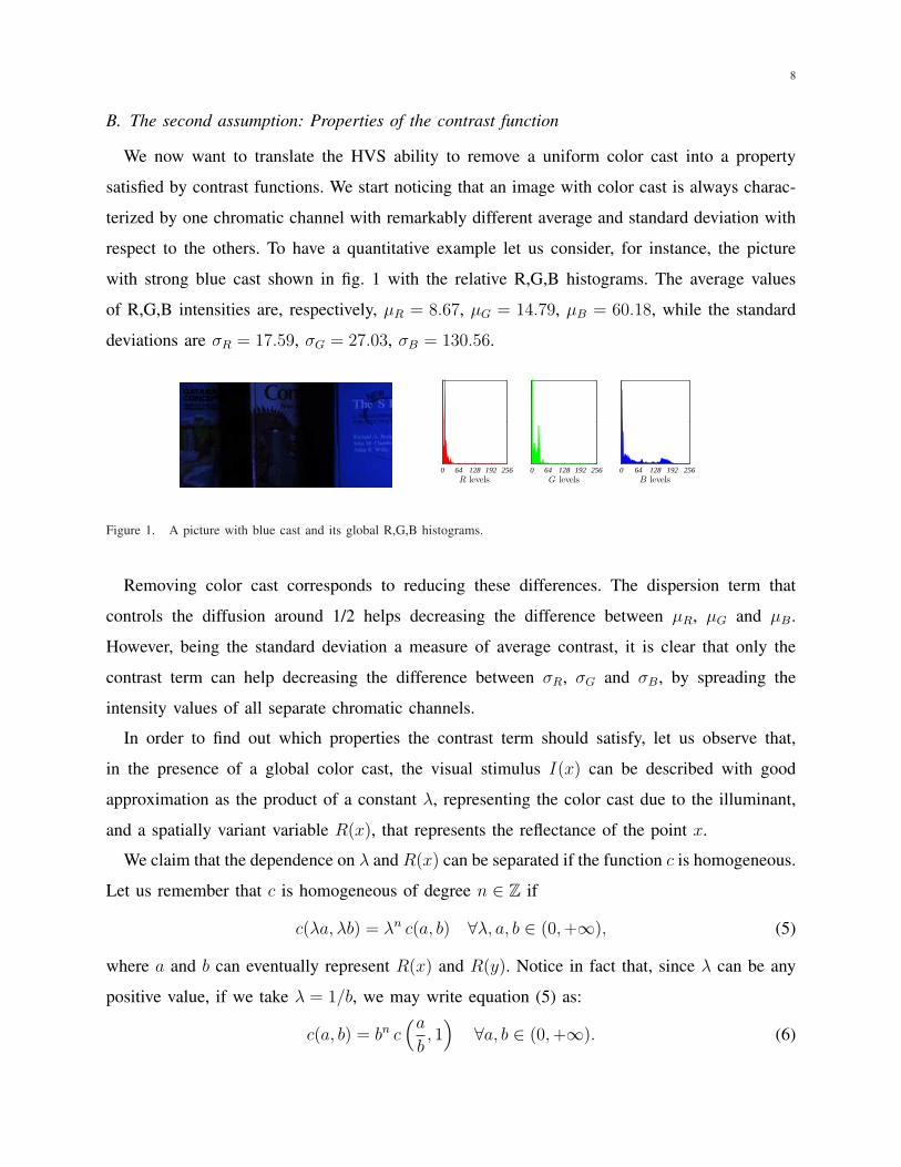
with strong blue cast shown in fig. 1 with the relative R,G,B histograms. The average values
of R,G,B intensities are, respectively, µR = 8.67, µG = 14.79, µB = 60.18, while the standard
deviations are σR = 17.59, σG = 27.03, σB = 130.56.
0 64 128 192 256R levels
0 64 128 192 256G levels
0 64 128 192 256B levels
Figure 1. A picture with blue cast and its global R,G,B histograms.
Removing color cast corresponds to reducing these differences. The dispersion term that
controls the diffusion around 1/2 helps decreasing the difference between µR, µG and µB.
However, being the standard deviation a measure of average contrast, it is clear that only the
contrast term can help decreasing the difference between σR, σG and σB, by spreading the
intensity values of all separate chromatic channels.
In order to find out which properties the contrast term should satisfy, let us observe that,
in the presence of a global color cast, the visual stimulus I(x) can be described with good
approximation as the product of a constant λ, representing the color cast due to the illuminant,
and a spatially variant variable R(x), that represents the reflectance of the point x.
We claim that the dependence on λ and R(x) can be separated if the function c is homogeneous.
Let us remember that c is homogeneous of degree n ∈ Z if
c(λa, λb) = λn c(a, b) ∀λ, a, b ∈ (0, +∞), (5)
where a and b can eventually represent R(x) and R(y). Notice in fact that, since λ can be any
positive value, if we take λ = 1/b, we may write equation (5) as:
c(a, b) = bn c(a
b, 1
)∀a, b ∈ (0, +∞). (6)
9
Hence, if c is a homogeneous function of degree n = 0, then bn = 1, so that c is a function
of the ratio a/b and intrinsically disregards the color cast. If n > 0, then the cast has a global
influence and could be removed performing a suitable normalization (for instance, dividing by
the n-th power of the highest intensity level). We can formalize these considerations in our
second assumption.
Assumption 2. In order to remove the color cast, we assume that the inverse contrast function
c(a, b) is homogeneous.
Thanks to the arguments presented so far, we have that inverse contrast functions which are
homogeneous of degree n = 0 are those that can be written as a monotone non-decreasing
function of min(I(x),I(y))max(I(x),I(y))
. It would be interesting to know if, given an inverse contrast function c,
there are increasing functions g, h : (0, +∞) → (0, +∞) such that g(c(h(a), h(b))) = ab, for any
0 < a < b. Probably some other assumptions on c are required to obtain such a characterization,
which means that, modulo a calibration of intensity values, min(I(x),I(y))max(I(x),I(y))
is the essential inverse
contrast function. In the next subsection we provide further support to restrict ourselves to such
class of contrast functions.
C. Contrast functions satisfying the Weber-Fechner’s law
Weber-Fechner’s law describes a common behavior of human senses. It has been first discov-
ered by Weber and then formalized by Fechner. In general, it describes a non-linear response of
a human sense to variations of external stimuli: the same variation is perceived in a weaker way
as the strength of the external stimulus increases. The experiment for human vision is performed
in controlled conditions [17]: on a uniform background of intensity I0, it is superimposed a brief
pulse of light of intensity I1 > I0. Weber-Fechner’s law states that the so-called Weber-Fechner
ratio RWF ≡ I1−I0I0
, i.e. the ratio between the variation ∆I ≡ I1 − I0 and the background
I0, remains constant. Even though Weber-Fechner’s law is not perfect [4], the intensity range
over which it is in good agreement with experience (called ‘Weber-Fechner’s domain’) is still
comparable to the dynamic range of most electronic imaging systems [4].
Since RWF = I1/I0−1, Weber-Fechner’s law is saying that the perceived contrast is a function
of I1/I0. This reason motivates us to say that c(a, b) is a generalized Weber-Fechner contrast
10
function if c is an inverse contrast function which can be written as a non-decreasing function
of min(a, b)/ max(a, b). Hence, we can particularize assumption 2 as follows.
Assumption 2’. We assume that c is a generalized Weber-Fechner contrast function.
IV. EXPLICIT ENERGY FUNCTIONALS COMPLYING WITH OUR SET OF ASSUMPTIONS
The purpose of this section is to show explicit examples of energy functionals complying with
our set of assumptions. We first concentrate on the contrast terms, then we discuss the dispersion
terms and, finally, we analyze the Euler-Lagrange equations of the complete energy functionals.
Here we mainly concentrate on mathematical features, reserving qualitative interpretations and
comparisons for the following section.
A. Three basic inverse contrast terms
As we have explained in Section III we shall concentrate on generalized Weber-Fechner
contrast terms. The following three are of particular interest:
C idw (I) :=
1
4
∑
x∈I
∑
y∈I
w(x, y)min(I(x), I(y))
max(I(x), I(y)), (7)
C logw (I) :=
1
4
∑
x∈I
∑
y∈I
w(x, y) log
(min(I(x), I(y))
max(I(x), I(y))
), (8)
C −Mw (I) := −1
4
∑
x∈I
∑
y∈I
w(x, y)M(
min(I(x), I(y))
max(I(x), I(y))
), (9)
where
M(
min(I(x), I(y))
max(I(x), I(y))
):=
1− min(I(x),I(y))max(I(x),I(y))
1 + min(I(x),I(y))max(I(x),I(y))
≡ |I(x)− I(y)|I(x) + I(y)
, (10)
is the well known Michelson’s definition of contrast [24]. The upper symbol in the above
definitions of Cw simply specifies the monotone function applied on the basic contrast variable
t := min(I(x),I(y))max(I(x),I(y))
, i.e. identity id(t) = t, logarithm log t, and minus the Michelson’s contrast
function −M(t) = −1−t1+t
, respectively. Indeed, these three functions are strictly increasing (this
is obvious for the first two, for the third observe that −M′(t) = 2/(1+ t)2 > 0 for all t). Notice
that the function t = min(I(x), I(y))/ max(I(x), I(y)) is minimized when min(I(x), I(y))
takes the smallest possible value and max(I(x), I(y)) takes the largest possible one, which
11
corresponds to a contrast stretching. Thus, minimizing an increasing function of the variable t,
we produce a contrast enhancement. To refer to any one of them we use the notation Cfw(I),
where f = id, log,−M.
Let us briefly comment on the reasons for considering those contrast terms among others in
the Weber-Fechner class. The first one is the simplest, and it is useful to understand the basic
contrast enhancement properties of our energy functionals. The second has been chosen because
of the logarithmic property to transform ratios in differences, so that the basic contrast variable
becomes min(I(x), I(y))−max(I(x), I(y)) = −|I(x)− I(y)|, being I ≡ log I . Finally, the third
one has been chosen because it is given in terms of the integral of Michelson’s contrast.
B. Entropic dispersion term
The main features of the dispersion term have to be its attachment to the initial given image
I0 and to the average illumination value, which we assume to be 1/2. In principle, to measure
the dispersion of I with respect to I0 or 1/2, any distance function can be used. The simplest
example would be a quadratic distance
Dqα,β(I) :=
α
2
∑
x∈I
(I(x)− 1
2
)2
+β
2
∑
x∈I
(I(x)− I0(x))2 , α, β > 0. (11)
Given that contrast terms are expressed as homogeneous functions of degree 0, the variational
derivatives are homogeneous functions of degree -1 (see Appendix IX-C). Since our axioms
do not give any precise indication about the analytical form of the dispersion term that should
be chosen, we search for functions able to maintain coherence with this homogeneity. A good
candidate for this is the entropic dispersion term, i.e.
DEα,β(I) := α
∑
x∈I
(1
2log
1
2I(x)−
(1
2− I(x)
))+ β
∑
x∈I
(I0(x) log
I0(x)
I(x)− (I0(x)− I(x))
),
(12)
where α, β > 0, which is based on the relative entropy distance [25] between I and 1/2 (the first
term) and between I0 and I(the second term). Notice that, if a > 0 and f(s) = a log as− (a− s),
s ∈ (0, 1], then dfds
(s) = 1 − as
and d2fds2 (s) = a
s2 > 0, ∀s. So, f(s) has a global minimum in
s = a. In particular, this holds when a = I0(x) or a = 1/2. Given the statistical interpretation
of entropy, we can say that minimizing DEα,β(I) amounts to minimizing the disorder of intensity
levels around 1/2 and around the original data I0(x). Thus, DEα,β(I) accomplishes the required
tasks of a dispersion term.
12
0 0.2 0.4 0.6 0.8 10
0.2
0.4
0.6
0.8
1
1.2
1.4
1.6
1.8
2
Normalized intensity
Ent
ropi
c vs
. qua
drat
ic d
ispe
rsio
n st
reng
th
Entropic dispersionQuadratic dispersion
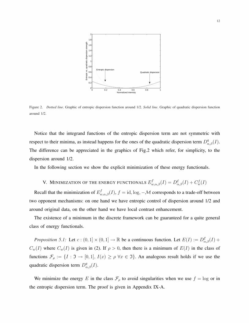
Figure 2. Dotted line. Graphic of entropic dispersion function around 1/2. Solid line. Graphic of quadratic dispersion function
around 1/2.
Notice that the integrand functions of the entropic dispersion term are not symmetric with
respect to their minima, as instead happens for the ones of the quadratic dispersion term Dqα,β(I).
The difference can be appreciated in the graphics of Fig.2 which refer, for simplicity, to the
dispersion around 1/2.
In the following section we show the explicit minimization of these energy functionals.
V. MINIMIZATION OF THE ENERGY FUNCTIONALS Efw,α,β(I) = DE
α,β(I) + Cfw(I)
Recall that the minimization of Efw,α,β(I), f = id, log,−M corresponds to a trade-off between
two opponent mechanisms: on one hand we have entropic control of dispersion around 1/2 and
around original data, on the other hand we have local contrast enhancement.
The existence of a minimum in the discrete framework can be guaranteed for a quite general
class of energy functionals.
Proposition 5.1: Let c : (0, 1]× (0, 1] → R be a continuous function. Let E(I) := DEα,β(I) +
Cw(I) where Cw(I) is given in (2). If ρ > 0, then there is a minimum of E(I) in the class of
functions Fρ := {I : I → [0, 1], I(x) ≥ ρ ∀x ∈ I}. An analogous result holds if we use the
quadratic dispersion term Dqα,β(I).
We minimize the energy E in the class Fρ to avoid singularities when we use f = log or in
the entropic dispersion term. The proof is given in Appendix IX-A.
13
Notice that if the energy E is differentiable the minimum I∗ satisfies δE(I∗) = 0. Before com-
puting the Euler-Lagrange equations, we notice that the contrast terms Cfw(I), f = id, log,−M
are not convex and the basic function t := min(a,b)max(a,b)
is not differentiable. In fact, we may write
min(a, b) = 12(a + b − |a − b|), max(a, b) = 1
2(a + b + |a − b|), for any a, b ∈ R. The non-
differentiability comes from the absolute value A(z) = |z|, z ∈ R. Since our algorithm will use
a gradient descent approach, we must regularize the basic variable t. We notice that A′(z) = 1
if z > 0, A′(z) = −1 if z < 0 and A is not differentiable at z = 0. But all the values s ∈ [−1, 1]
are subtangents of A(z) at z = 0, that is, A(z)−A(0) ≥ s(z− 0) for any z ∈ R. Thus we may
write A′(z) = sign(z), where
sign(z) =
1 if z > 0
[−1, 1] if z = 0
−1 if z < 0
. (13)
We define sign0(z) as in (13), but with the particular choice 0 when z = 0.
Def. 5.1: Given ε > 0, we say that Aε(z) is a ‘nice regularization’ of A(z), if Aε(z) ≥ 0 is
convex, differentiable with continuous derivative, Aε(0) = 0, Aε(−z) = Aε(z), and
(i) Aε(z) ≤ |z| for any z ∈ R and Aε(z) = |z|+Q1,ε(z) where Q1,ε(z) → 0 as ε → 0, uniformly
in z ∈ [−1, 1];
(ii) Let us denote sε(z) = A′ε(z). Then |sε(z)| ≤ 1 for any z ∈ [−1, 1], sε(z) → sign0(z) as
ε → 0 for any z ∈ R, and Q2,ε(z) := Aε(z)− zsε(z) → 0 as ε → 0, uniformly in z ∈ [−1, 1].
We present two examples of nice regularization of A(z). Example a): Aε(z) =√
ε2 + |z|2− ε,
in this case sε(z) = z√ε2+|z|2 , Q1,ε(z) = O(ε) and Q2,ε(z) := Aε(z) − zsε(z) = O(ε). Example
b): Aε(z) = z arctan(z/ε)arctan(1/ε)
− ε2 arctan(1/ε)
log(1 + z2
ε2), in this case sε(z) = arctan(z/ε)
arctan(1/ε), Q1,ε(z) =
O(ε log (1/ε)) and Q2,ε(z) = O(ε log (1/ε)), uniformly in z ∈ [−1, 1]. We have denoted by
O(F (ε)) any expression satisfying |O(F (ε))| ≤ CF (ε) for some constant C > 0 and ε > 0
small enough. Observe that, in both cases sε(z) → sign0(z) as ε → 0 for any z ∈ R. We give
the details of the above statements in Appendix IX-B.
Now let us assume that Aε(z) is a nice regularization of A(z). We set
minε(a, b) =1
2(a + b− Aε(a− b)), maxε(a, b) =
1
2(a + b + Aε(a− b)). (14)
14
We define the regularized version of the functionals as:
C idw,ε(I) :=
1
4
∑
x∈I
∑
y∈I
w(x, y)minε(I(x), I(y))
maxε(I(x), I(y)); (15)
C logw,ε (I) :=
1
4
∑
x∈I
∑
y∈I
w(x, y) log
(minε(I(x), I(y))
maxε(I(x), I(y))
); (16)
C −Mw,ε (I) := −1
4
∑
x∈I
∑
y∈I
w(x, y)Aε(I(x)− I(y))
I(x) + I(y). (17)
Proposition 5.2: Assume that Aε(z) is a nice regularization of A(z).
(i) The first variation of C idw,ε(I) is:
δC idw,ε(I) = −1
2
∑y∈I w(x, y) I(y)
maxε(I(x),I(y))2sε(I(x)− I(y)) + Sε
= −12
∑y∈I w(x, y) I(y)
max(I(x),I(y))2sε(I(x)− I(y)) + S ′ε,
(18)
where Sε, S′ε = O(Q1,ε(I(x)− I(y)) + Q2,ε(I(x)− I(y)));
(ii) The first variation of C logw,ε (I) is:
δC logw,ε (I) = −1
2
∑
y∈I
w(x, y)1
I(x)sε(I(x)− I(y)) + Sε, (19)
where Sε = O(Q1,ε(I(x)− I(y)) + Q2,ε(I(x)− I(y)));
(iii) The first variation of C−Mw,ε (I) is:
δC−Mw,ε (I) = −
∑
y∈I
w(x, y)I(y)
(I(x) + I(y))2sε(I(x)− I(y)) + Sε, (20)
where Sε = O(Q2,ε(I(x)− I(y))).
In all cases Q1,ε(z), Q2,ε(z) → 0 as ε → 0, uniformly in z ∈ [−1, 1].
Thus we know that Sε = O(ε) if Aε(z) is given by Example a), and Sε = O(ε log 1/ε) if
Aε(z) is given by Example b). These are the cases of interest for us in the experiments.
The proof of this proposition will be given in Appendix IX-C.
15
Notice that, letting ε → 0 we have that δCfw,ε(I) → δCf
w,0(I), where
δC idw,0(I) = −1
2
∑
y∈I
w(x, y)I(y)
max(I(x), I(y))2sign0(I(x)− I(y))
= −1
2
∑
{y∈I : I(x)>I(y)}w(x, y)
I(y)
I(x)2−
∑
{y∈I : I(x)<I(y)}w(x, y)
1
I(y)
;
δC logw,0(I) = −1
2
∑
y∈I
w(x, y)1
I(x)sign0(I(x)− I(y))
= −1
2
∑
{y∈I : I(x)>I(y)}w(x, y)
1
I(x)−
∑
{y∈I : I(x)<I(y)}w(x, y)
1
I(x)
;
δC −Mw,0 (I) = −
∑
y∈I
w(x, y)I(y)
(I(x) + I(y))2sign0(I(x)− I(y))
= −∑
{y∈I : I(x)>I(y)}w(x, y)
I(y)
(I(x) + I(y))2+
∑
{y∈I : I(x)<I(y)}w(x, y)
I(y)
(I(x) + I(y))2.
Now, by direct computation, we have that the derivative of the entropic dispersion term is:
δDEα,β(I) = α
(1− 1
2I(x)
)+ β
(1− I0(x)
I(x)
). (21)
We can see that this expression has a degree of homogeneity -1 with respect to I(x), the same
as the variation of the three contrast terms Cfw(I).
Assume that α, β > 0 are fixed. If Efw,ε(I) = DE
α,β(I) + Cfw,ε(I), f = id, log, −M, then by
linearity of the variational derivative, we have δEfw,ε(I) = δDE
α,β(I) + δCfw,ε(I). The minimum
of Efw,ε(I) satisfies δEf
w,ε(I) = 0. To search for the minimum we use a semi-implicit discrete
gradient descent strategy with respect to log I . The continuous gradient descent equation is
∂t log I = −δEfw,ε(I), (22)
being t the evolution parameter. Since ∂t log I = 1I∂tI , we have
∂tI = −IδEfw,ε(I). (23)
Using the gradient descent in log I leads to (23), which is related to a gradient descent approach
which uses the relative entropy as a metric, instead of the usual quadratic distance (see [25]).
16
Let us now discretize our scheme: choosing a finite evolution step ∆t > 0 and setting Ik(x) =
Ik∆t(x), k = 0, 1, 2, . . ., being I0(x) the original image, thanks to (21), we can write the semi-
implicit discretization of (23) as
Ik+1(x)− Ik(x)
∆t= α
(1
2− Ik+1(x)
)+ β
(I0(x)− Ik+1(x)
)− Ik(x)δC fw,ε(I
k). (24)
Now, considering the explicit expressions of δC fw,ε(I
k), neglecting their second terms containing
Sε (see Proposition 5.2 (i),(ii),(iii)) and performing some easy algebraic manipulations, we find
the equation
Ik+1(x) =Ik(x) + ∆t
(α2
+ βI0(x) + 12R f
ε,Ik(x))
1 + ∆t(α + β), (25)
where the function R fε,Ik(x) assumes three different forms for f = id, log, −M, precisely
R idε,Ik(x) := −2IkδC id
w,ε(Ik) =
∑
y∈I
w(x, y)Ik(x)Ik(y)
maxε(Ik(x), Ik(y))2sε(I
k(x)− Ik(y)). (26)
R logε,Ik(x) := −2IkδC log
w,ε(Ik) =
∑
y∈I
w(x, y) sε(Ik(x)− Ik(y)). (27)
RMε,Ik(x) := −2IkδC−M
w,ε (Ik) =∑
y∈I
w(x, y)2Ik(x)Ik(y)
(Ik(x) + Ik(y))2sε(I
k(x)− Ik(y)). (28)
At the limit ε → 0 we have:
R id0,Ik(x) =
∑
{y∈I : I(x)>I(y)}w(x, y)
Ik(y)
Ik(x)+
∑
{y∈I : I(x)<I(y)}w(x, y)
Ik(x)
Ik(y). (29)
R log0,Ik(x) =
∑
y∈I
w(x, y) sign0(Ik(x)− Ik(y)). (30)
R−M0,Ik (x) =
∑
I
w(x, y)2Ik(x)Ik(y)
(Ik(x) + Ik(y))2sign0(I
k(x)− Ik(y)). (31)
In Appendix IX-D, we will comment on the stability of these iterative methods.

17
VI. FEATURES OF THE THREE COMPUTATIONAL ALGORITHMS AND COMPARISON WITH
EXISTING MODELS
Equation (25) can be used to implement three iterative computational algorithms for color
image enhancement, as f varies. Notice that the R functions share an identical structure, i.e.
Rfε,Ik(x) =
∑y∈I w(x, y) rf
ε (Ik(x), Ik(y)), for a suitable function rfε . In Fig. 3 we show the
surfaces representing their graphics.
We can see that the surfaces representing ridε and r−Mε are very similar, the only difference
being that the second is quite smoother than the first. Hence, we expect the corresponding
algorithms to have similar enhancing properties.
Instead, the surface representing rlogε shows an opposite behavior with respect to the previous
two surfaces at the extreme points. Moreover, since the logarithmic function grows very rapidly
for small values of its argument and slowly for higher ones, we expect the corresponding
algorithm to perform a strong contrast enhancement in dark image areas and a weak one in
bright zones. In section VIII it will be shown that all these observations are verified by empirical
tests.
Figure 3. Left: Surface of ridε . Center: Surface of rlog
ε . Right: Surface of r−Mε . Corresponding to the function sε(z) =
arctan(z/ε)/ arctan(1/ε) with ε = 1/20.
We now want to show that there is a precise correspondence between the algorithm corre-
sponding to E logw,ε and ACE [13], a recent perceptually inspired color correction algorithm, while
the algorithms corresponding to the energies E idw,ε, E−M
w,ε are qualitatively related with the Retinex
model, but they also exhibit new peculiarities that distinguish them from Retinex.
18
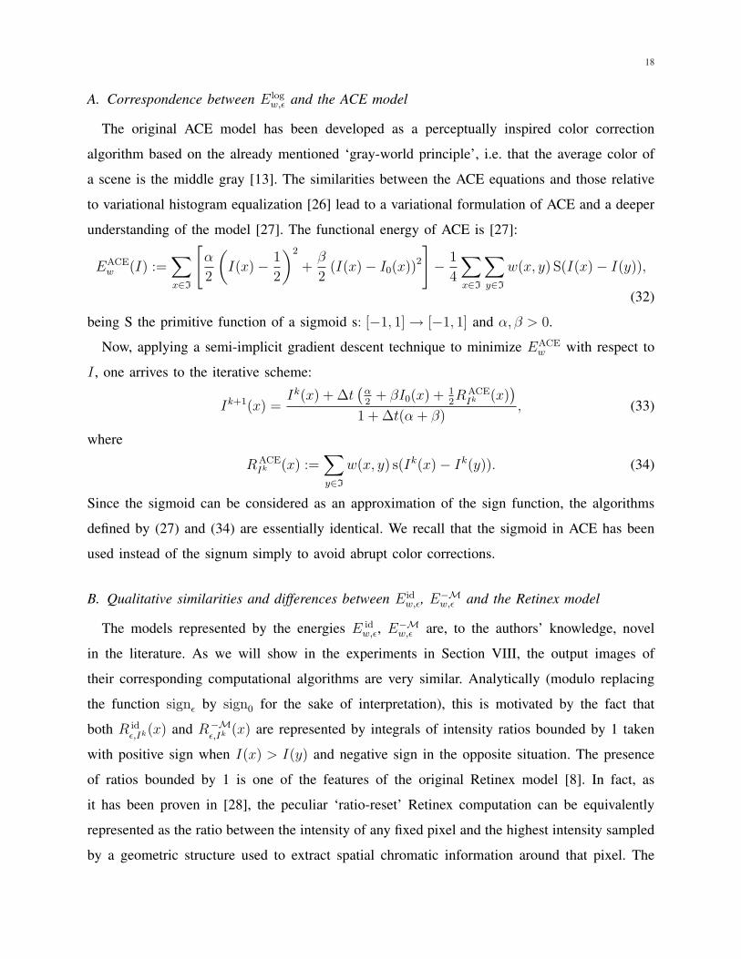
A. Correspondence between Elogw,ε and the ACE model
The original ACE model has been developed as a perceptually inspired color correction
algorithm based on the already mentioned ‘gray-world principle’, i.e. that the average color of
a scene is the middle gray [13]. The similarities between the ACE equations and those relative
to variational histogram equalization [26] lead to a variational formulation of ACE and a deeper
understanding of the model [27]. The functional energy of ACE is [27]:
EACEw (I) :=
∑
x∈I
[α
2
(I(x)− 1
2
)2
+β
2(I(x)− I0(x))2
]− 1
4
∑
x∈I
∑
y∈I
w(x, y) S(I(x)− I(y)),
(32)
being S the primitive function of a sigmoid s: [−1, 1] → [−1, 1] and α, β > 0.
Now, applying a semi-implicit gradient descent technique to minimize EACEw with respect to
I , one arrives to the iterative scheme:
Ik+1(x) =Ik(x) + ∆t
(α2
+ βI0(x) + 12RACE
Ik (x))
1 + ∆t(α + β), (33)
where
RACEIk (x) :=
∑
y∈I
w(x, y) s(Ik(x)− Ik(y)). (34)
Since the sigmoid can be considered as an approximation of the sign function, the algorithms
defined by (27) and (34) are essentially identical. We recall that the sigmoid in ACE has been
used instead of the signum simply to avoid abrupt color corrections.
B. Qualitative similarities and differences between Eidw,ε, E−M
w,ε and the Retinex model
The models represented by the energies E idw,ε, E−M
w,ε are, to the authors’ knowledge, novel
in the literature. As we will show in the experiments in Section VIII, the output images of
their corresponding computational algorithms are very similar. Analytically (modulo replacing
the function signε by sign0 for the sake of interpretation), this is motivated by the fact that
both R idε,Ik(x) and R−M
ε,Ik (x) are represented by integrals of intensity ratios bounded by 1 taken
with positive sign when I(x) > I(y) and negative sign in the opposite situation. The presence
of ratios bounded by 1 is one of the features of the original Retinex model [8]. In fact, as
it has been proven in [28], the peculiar ‘ratio-reset’ Retinex computation can be equivalently
represented as the ratio between the intensity of any fixed pixel and the highest intensity sampled
by a geometric structure used to extract spatial chromatic information around that pixel. The
19
geometric structures used in the various Retinex implementations are many: paths, masks, sprays,
etc. See, e.g., [29] for a more detailed overview.
The fundamental difference between Retinex and equations (26) and (28) is that, in the Retinex
model, ratios are performed only over the highest intensity value and they are always taken with
positive sign. As a consequence, as proved in [28], the ratio-reset Retinex operation is unbalanced,
i.e. it always increases the intensity of any pixel (a post-LUT processing can overcome this
problem, but this operation is not intrinsically contained in the ratio-reset Retinex equations).
Instead, equations (26) and (28) can both increase or reduce pixel intensity. For this reason, the
energies E idw,ε, E−M
w,ε , could be qualitatively thought as describing a ‘symmetrized Retinex model’.
Later we will compare the action of this model with the one of Retinex on an overexposed image,
exhibiting the advantages provided by the symmetrization just commented.
VII. A GENERAL STRATEGY FOR COMPUTATIONAL COMPLEXITY REDUCTION
The computational complexity of the algorithms derived from the minimization of the energy
functionals that we have examined is O(N2), N being the number of pixels of the input image.
In fact, the computational complexity of R idε,Ik(x), R log
ε,Ik(x) and R−Mε,Ik (x) is of order O(N) for
every x, hence the global computational complexity is of order O(N2). This implies that with
a standard PC (P4, 3GHz) it can take up hours to process a high resolution image.
In [29] a local sampling technique has been devised to reduce time computation. Here we
provide a different technique, based on mathematical properties of the r-functions rather that on
sampling. This permits to maintain all the chromatic information, avoiding sampling noise.
From now on, we assume that w is a function of ‖x − y‖I and we show how to speed up
the computation of Rfε,Ik(x), reducing its computational complexity to O(N log N) by means
of a suitable approximation, which generalizes an analogous technique used in [27] to speed
up the ACE algorithm. Let us denote with R(x) =∑
y∈I w(x, y) r(I(x), I(y)) any of the three
R-functions specified in equations (26), (27), (28), omitting the indexes f , ε and Ik both to
simplify the notation and because their specification is not important for what follows.
The basic observation underlying our proposal is that, if we manage to separate the dependence
of the function r on I(x) and I(y), then we can express R(x) as a sum of convolutions. In
fact, let us suppose that R(x) admits a polynomial approximation R(n)(x), being n ∈ N the

20
approximation degree, such as
R(n)(x) =n∑
j=0
fj(I(x))∑
y∈I
w(x, y) gj(I(y)) , (35)
where fj are functions of I(x) and gj are functions of I(y). Since w is a function of x − y,
it is clear that the integrals appearing in (35) actually reduce to convolutions, which can be
computed using the Fast Fourier Transform (FFT), whose computational complexity is of order
O(N log N). Hence, if n << N , the computational complexity of the approximated algorithm
reduces to O(N log N).
To achieve the separation of variables in (35), we fix an approximation degree n and we use
a numerical algorithm to find the polynomial p(I(x), I(y)) =∑n
j=0
∑jl=0 pj−l,l I(x)j−l I(y)l,
pj−l,l ∈ R, that minimizes the L2 distance to r(I(x), I(y)). Indeed, since r is computed only
once (before the first gradient descent iteration,) we can choose the degree n to control the
maximum error. The polynomial can be easily rearranged and expressed as p(I(x), I(y)) =∑n
j=0 fj(I(x)) I(y)j for suitable functions fj(I(x)). This expression can be directly used in
equation (35) setting gj(I(y)) ≡ Ij(y) for every j = 1, . . . , n. Increasing n, one can reduce the
approximation error; our experiments show that for the functions ridε , rlog
ε and r−Mε , the value
n = 9 gives a satisfactory approximation, so we have used it in all of our tests.
For the sake of completeness, we notice that, if the surface representing the function r(I(x), I(y))
has discontinuities or strong gradients, a polynomial expansion may not be useful for its approx-
imation. In such a case, a Fourier expansion could be more suitable than the polynomial one,
but the corresponding expression of gj(I(y)) would be analytically more complicated, being, in
this case, expressed in terms of trigonometric functions instead of powers.
VIII. TESTS
So far, we have performed a theoretical investigation about the proposed axiomatic framework
for perceptually inspired variational color enhancement. In this section, we show and discuss
some tests about the algorithms derived from the three functional energies examined. Before
going into details, it is worthwhile to recall that the algorithms represented by equations (25),
(26), (27) and (28) have four explicit parameters: α, β, ε and ∆t, moreover, the function w
determines the local contrast enhancement behavior. We have chosen the function w(x, y) =
A‖x−y‖I
, where A is the normalization parameter, so that (1) is satisfied. Recall that α controls
21
the dispersion around the middle gray, β sets the strength of attachment to original data, and ∆t
is the gradient descent step. The parameter ε controls the regularization of the signum function.
In practice, we have chosen sε(z) = arctan(z/ε)/ arctan(1/ε) because the signum function is
too singular to be used without leading to unwanted noise amplification.
Our tests indicate that an overall satisfactory set of parameters is α = 255253
, β = 1, ∆t = 0.2,
and ε = 120
. We iterate until the average Mean Square Error (MSE) per pixel (between the images
in the current and previous iteration) falls below a threshold of 10−4 (typically the steady state is
reached within 10-20 iterations.) Varying these parameters with respect to image characteristics
could possibly give better results. We consider the image-dependency of parameters an interesting
issue to be investigated, but its thorough and significative analysis falls outside the scope of this
paper.
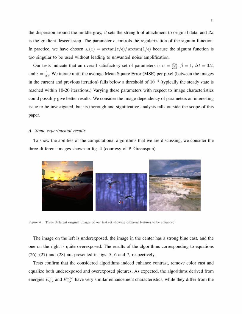
A. Some experimental results
To show the abilities of the computational algorithms that we are discussing, we consider the
three different images shown in fig. 4 (courtesy of P. Greenspun).
Figure 4. Three different original images of our test set showing different features to be enhanced.
The image on the left is underexposed, the image in the center has a strong blue cast, and the
one on the right is quite overexposed. The results of the algorithms corresponding to equations
(26), (27) and (28) are presented in figs. 5, 6 and 7, respectively.
Tests confirm that the considered algorithms indeed enhance contrast, remove color cast and
equalize both underexposed and overexposed pictures. As expected, the algorithms derived from
energies E idw,ε and E−M
w,ε have very similar enhancement characteristics, while they differ from the
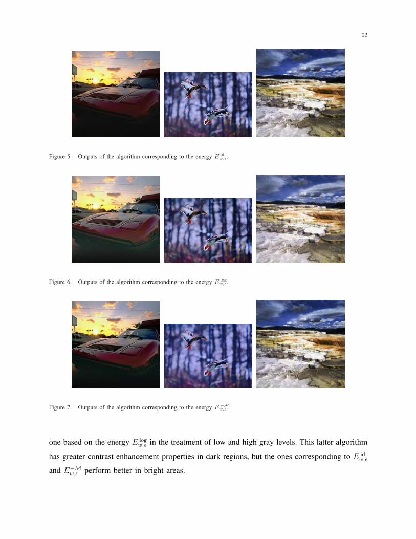
22
Figure 5. Outputs of the algorithm corresponding to the energy E idw,ε.
Figure 6. Outputs of the algorithm corresponding to the energy E logw,ε .
Figure 7. Outputs of the algorithm corresponding to the energy E −Mw,ε .
one based on the energy E logw,ε in the treatment of low and high gray levels. This latter algorithm
has greater contrast enhancement properties in dark regions, but the ones corresponding to E idw,ε
and E−Mw,ε perform better in bright areas.
23
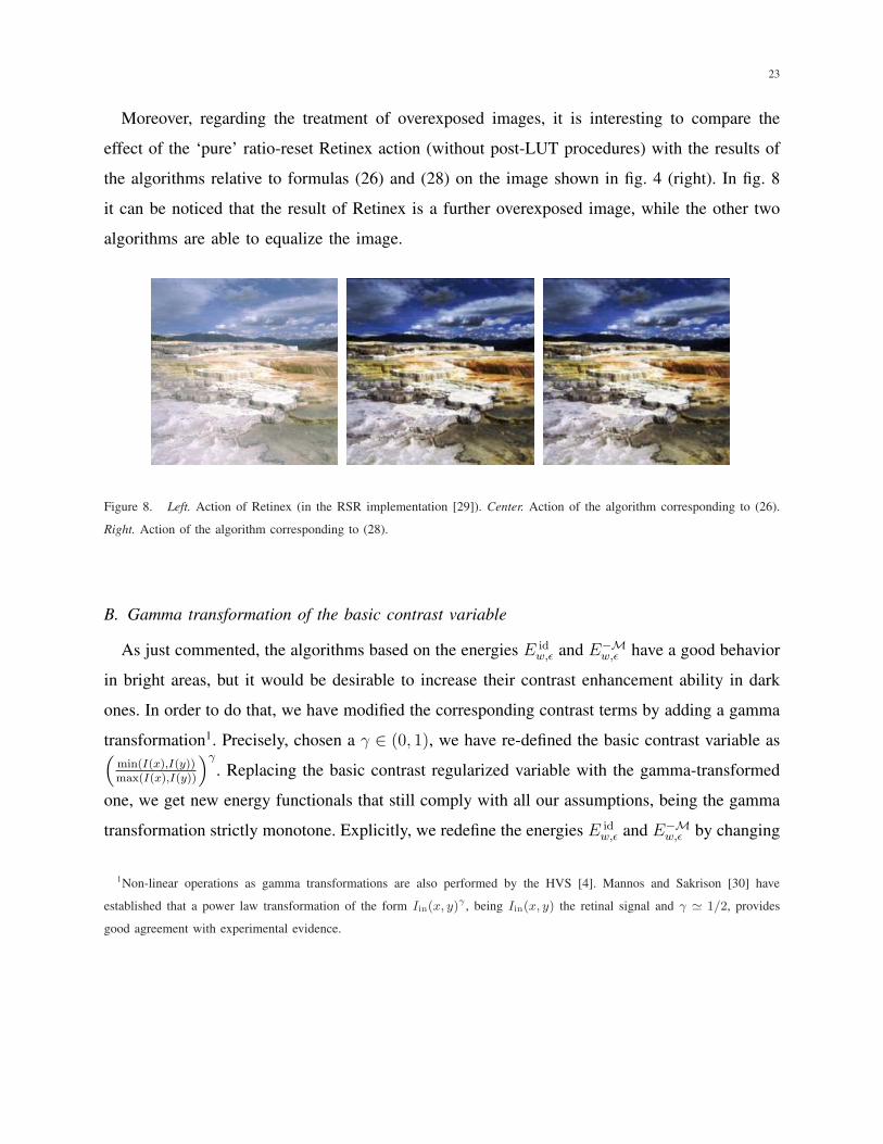
Moreover, regarding the treatment of overexposed images, it is interesting to compare the
effect of the ‘pure’ ratio-reset Retinex action (without post-LUT procedures) with the results of
the algorithms relative to formulas (26) and (28) on the image shown in fig. 4 (right). In fig. 8
it can be noticed that the result of Retinex is a further overexposed image, while the other two
algorithms are able to equalize the image.
Figure 8. Left. Action of Retinex (in the RSR implementation [29]). Center. Action of the algorithm corresponding to (26).
Right. Action of the algorithm corresponding to (28).
B. Gamma transformation of the basic contrast variable
As just commented, the algorithms based on the energies E idw,ε and E−M
w,ε have a good behavior
in bright areas, but it would be desirable to increase their contrast enhancement ability in dark
ones. In order to do that, we have modified the corresponding contrast terms by adding a gamma
transformation1. Precisely, chosen a γ ∈ (0, 1), we have re-defined the basic contrast variable as(min(I(x),I(y))max(I(x),I(y))
)γ
. Replacing the basic contrast regularized variable with the gamma-transformed
one, we get new energy functionals that still comply with all our assumptions, being the gamma
transformation strictly monotone. Explicitly, we redefine the energies E idw,ε and E−M
w,ε by changing
1Non-linear operations as gamma transformations are also performed by the HVS [4]. Mannos and Sakrison [30] have
established that a power law transformation of the form Iin(x, y)γ , being Iin(x, y) the retinal signal and γ ' 1/2, provides
good agreement with experimental evidence.
24
the contrast terms C idw,ε and C−M
w,ε by the gamma-transformed ones2
C idw,ε,γ(I) =
1
4γ
∑
x∈I
∑
y∈I
w(x, y)
(minε(I(x), I(y))
maxε(I(x), I(y))
)γ
; (36)
C −Mw,ε,γ(I) = − 1
4γ
∑
x∈I
∑
y∈I
w(x, y)Aε(I(x)γ − I(y)γ)
I(x)γ + I(y)γ. (37)
By direct computation, it can be seen that the gradient descent equations corresponding to the
gamma-transformed contrast terms still have the general form represented by equation (25), but
now with these new R-functions
R idε,γ,Ik(x) :=
∑
y∈I
w(x, y)
(minε(I
k(x), Ik(y))
maxε(Ik(x), Ik(y))
)γ
sε(Ik(x)− Ik(y)), (38)
R−Mε,γ,Ik(x) :=
∑
y∈I
w(x, y)2
(minε(I
k(x), Ik(y))γ maxε(Ik(x), Ik(y))γ
)
(minε(Ik(x), Ik(y))γ + maxε(Ik(x), Ik(y))γ)2 sε(Ik(x)−Ik(y)). (39)
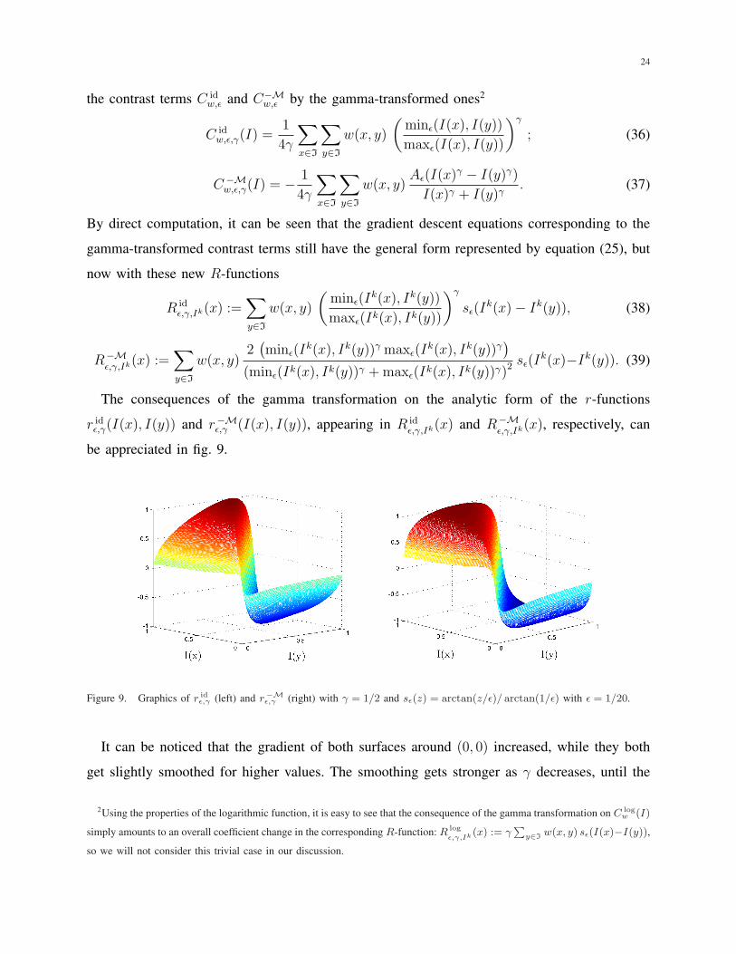
The consequences of the gamma transformation on the analytic form of the r-functions
r idε,γ(I(x), I(y)) and r−Mε,γ (I(x), I(y)), appearing in R id
ε,γ,Ik(x) and R−Mε,γ,Ik(x), respectively, can
be appreciated in fig. 9.
Figure 9. Graphics of r idε,γ (left) and r−Mε,γ (right) with γ = 1/2 and sε(z) = arctan(z/ε)/ arctan(1/ε) with ε = 1/20.
It can be noticed that the gradient of both surfaces around (0, 0) increased, while they both
get slightly smoothed for higher values. The smoothing gets stronger as γ decreases, until the
2Using the properties of the logarithmic function, it is easy to see that the consequence of the gamma transformation on C logw (I)
simply amounts to an overall coefficient change in the corresponding R-function: R log
ε,γ,Ik (x) := γ∑
y∈I w(x, y) sε(I(x)−I(y)),
so we will not consider this trivial case in our discussion.
25
limit γ = 0, where they reduce to the same surface, precisely: r logε . The most suitable value of
γ depends on the image content, however our tests showed that an overall good performance
with γ = 1/2.
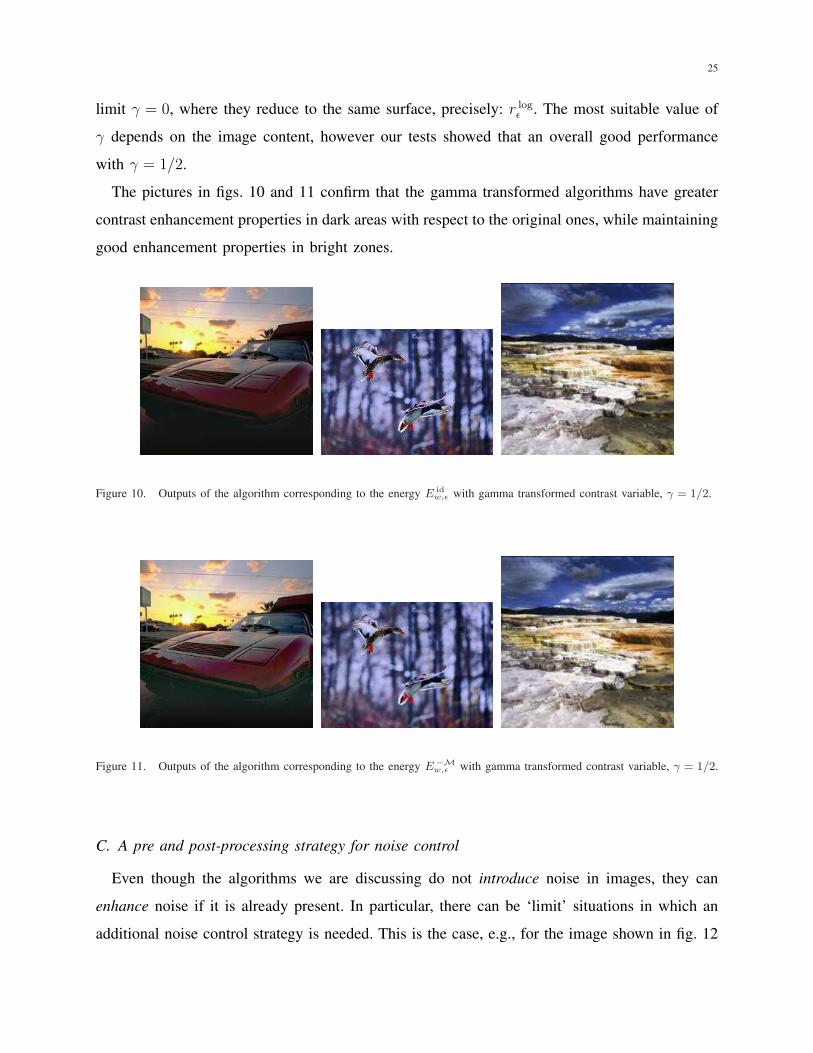
The pictures in figs. 10 and 11 confirm that the gamma transformed algorithms have greater
contrast enhancement properties in dark areas with respect to the original ones, while maintaining
good enhancement properties in bright zones.
Figure 10. Outputs of the algorithm corresponding to the energy E idw,ε with gamma transformed contrast variable, γ = 1/2.
Figure 11. Outputs of the algorithm corresponding to the energy E −Mw,ε with gamma transformed contrast variable, γ = 1/2.
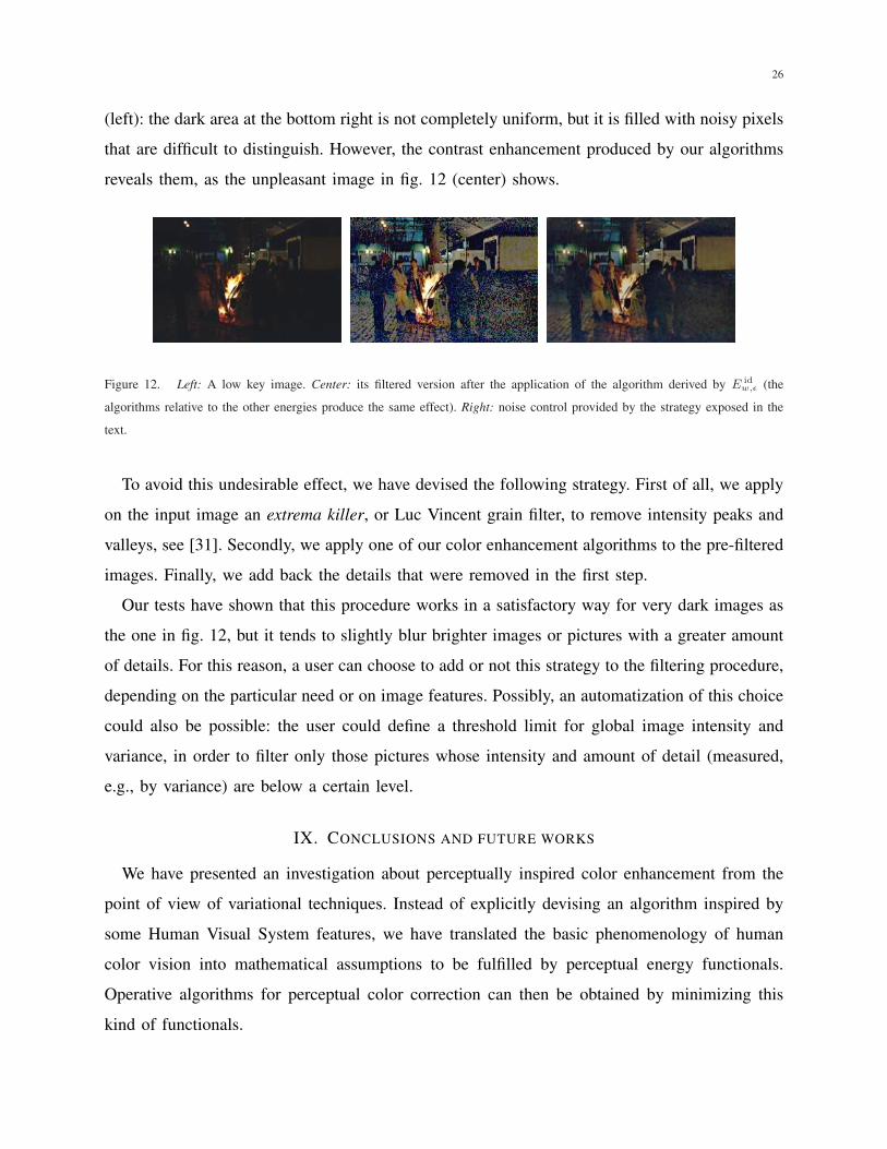
C. A pre and post-processing strategy for noise control
Even though the algorithms we are discussing do not introduce noise in images, they can
enhance noise if it is already present. In particular, there can be ‘limit’ situations in which an
additional noise control strategy is needed. This is the case, e.g., for the image shown in fig. 12
26
(left): the dark area at the bottom right is not completely uniform, but it is filled with noisy pixels
that are difficult to distinguish. However, the contrast enhancement produced by our algorithms
reveals them, as the unpleasant image in fig. 12 (center) shows.
Figure 12. Left: A low key image. Center: its filtered version after the application of the algorithm derived by E idw,ε (the
algorithms relative to the other energies produce the same effect). Right: noise control provided by the strategy exposed in the
text.
To avoid this undesirable effect, we have devised the following strategy. First of all, we apply
on the input image an extrema killer, or Luc Vincent grain filter, to remove intensity peaks and
valleys, see [31]. Secondly, we apply one of our color enhancement algorithms to the pre-filtered
images. Finally, we add back the details that were removed in the first step.
Our tests have shown that this procedure works in a satisfactory way for very dark images as
the one in fig. 12, but it tends to slightly blur brighter images or pictures with a greater amount
of details. For this reason, a user can choose to add or not this strategy to the filtering procedure,
depending on the particular need or on image features. Possibly, an automatization of this choice
could also be possible: the user could define a threshold limit for global image intensity and
variance, in order to filter only those pictures whose intensity and amount of detail (measured,
e.g., by variance) are below a certain level.
IX. CONCLUSIONS AND FUTURE WORKS
We have presented an investigation about perceptually inspired color enhancement from the
point of view of variational techniques. Instead of explicitly devising an algorithm inspired by
some Human Visual System features, we have translated the basic phenomenology of human
color vision into mathematical assumptions to be fulfilled by perceptual energy functionals.
Operative algorithms for perceptual color correction can then be obtained by minimizing this
kind of functionals.
27
The advantage to analyze perceptual energy functionals is that they can put in evidence in a
clearer way the action of color correction in terms of important image features such as, e.g.,
contrast and dispersion. In fact, our set of assumptions determines a particular class of functionals,
whose minimization corresponds to two opponent mechanisms: on one side a local and non-
linear contrast enhancement, on the other side a control of dispersion around the middle gray
and around the input image data values. The minimization is implemented through an iterative
gradient descent technique; the stability of this method and the existence of minima have been
proven.
We also pointed out theoretical similarities and differences between these models and existing
perceptual color correction models, Retinex and ACE, by identifying, in the class of perceptual
functionals, an energy functional that leads to ACE and one that corresponds to a sort of
symmetrization of Retinex.
Tests on different images confirm theoretical predictions about the proposed algorithms, which
can enhance details and remove color cast without introducing noise. However, already present
noise can eventually be amplified. For this reason we also provided a simple and fast pre and
post processing procedure that can be integrated in the algorithms to avoid noise amplification
in very dark images.
The algorithms depend on four explicit parameters with a clear meaning. Even though there
is a set of parameters that works in a satisfactory way for all images of our test set, an image
dependent tuning could possibly improve the enhancement characteristics. However, this tuning
is beyond the scope of this paper and we consider it as an open problem.
Finally, we believe that the noise control procedure presented in this paper can be improved,
e.g. treating the problem from a functional point of view and investigating the relationship
between noise and local spatial frequency.
ACKNOWLEDGMENTS
M. Bertalmıo and V. Caselles acknowledge partial support by PNPGC project, reference
MTM2006-14836, and IP-RACINE Project IST-511316. R. Palma acknowledges support by
Alfa CVFA, AML// 19.0902/97/0666/II-0366-FA. E. Provenzi acknowledges partial support by
PRIN-MIUR research project, 2005115173-002.

28
APPENDIX
A. The proof of Proposition 5.1
Notice that since c : (0, 1]×(0, 1] → R is continuous, then c(I(x), I(y)) is a bounded function
for any I ∈ Fρ := {I : I → [0, 1], I(x) ≥ ρ ∀x ∈ I}. Then the term Cw(I) is bounded in
Fρ. The same can be said of DEα,β(I). In particular, infI∈Fρ E(I) > −∞. Let Ik ∈ Fρ be a
minimizing sequence, i.e., assume that E(Ik) → infI∈Fρ E(I) as k →∞. Since Ik is uniformly
bounded and we are working in a finite dimensional space, there exists a subsequence, denote it
again by Ik, that converges to some I∞ ∈ Fρ. Since both terms DEα,β(I) and Cw(I) are continuous
in Fρ, then E(I∞) = infI∈Fρ E(I). The corresponding result for the quadratic dispersion term
Dqα,β(I) is proved in the same way.
B. Examples of nice regularization of the absolute value
Let us first check that the examples of regularization of A(z) given in subsection V are nice
regularization. Recall that we denote by O(F (ε)) any expression satisfying |O(F (ε))| ≤ CF (ε)
for some C > 0 and ε > 0 small enough. The examples are:
a) Aε(z) =√
ε2 + |z|2 − ε: in this case sε(z) = z√ε2+|z|2 . Then |Aε(z) − |z|| = ε + |z| −
√ε2 + |z|2 ≤ ε, that is Q1,ε(z) = O(ε). On the other hand, Q2,ε(z) := Aε(z) − zsε(z) =
ε2√ε2+z2 − ε = O(ε) as ε → 0 uniformly in z ∈ [−1, 1]. The other conditions are immediate and
we do not give the details.
b) Aε(z) = z arctan(z/ε)arctan(1/ε)
− ε2 arctan(1/ε)
log(1 + z2
ε2): in this case sε(z) = arctan(z/ε)
arctan(1/ε). Then
Aε(z) = |z|+ |z|(arctan(|z|/ε)− arctan(1/ε))
arctan(1/ε)− ε/2log(1 + z2
ε2)
arctan(1/ε).
Since we have for any z ∈ [−1, 1],
|arctan(1/ε)− arctan(|z|/ε)| =∫ 1/ε
|z|/ε
1
1 + s2ds ≤
∫ 1/ε
|z|/ε
1
s2ds = ε
(1
|z| − 1
),
we have
Q1,ε(z) = |Aε(z)− |z|| ≤ ε
arctan(1/ε)+
ε/2log(1 + z2
ε2)
arctan(1/ε)= O(ε log (1/ε))
uniformly in z ∈ [−1, 1]. Finally,
Q2,ε(z) = Aε(z)− zsε(z) = −ε/2log(1 + z2
ε2)
arctan(1/ε)= O(ε log (1/ε)),
29
uniformly in z ∈ [−1, 1]. Again, the other conditions are immediate and we do not give the
details.
C. The proof of Proposition 5.2
Before going into the proof of Proposition 5.2, in the following Lemma we compute the first
variation of a general functional in presence of symmetries.
Lemma 9.1: Let w : I2 → R be a symmetric function in (x, y) and F : (0,∞)2 → R be a
differentiable function in its variables (a, b). Assume that F is symmetric, i.e. F (a, b) = F (b, a)
for any (a, b) ∈ (0,∞)2. Let F1(a, b) = ∂F∂a
(a, b). Then, given
E(I) =
∫∫
I2
w(x, y)F (I(x), I(y))dxdy, (40)
its first variation can be written as
δE(I) = 2
∫
I
w(x, y)F1(I(x), I(y)) dy. (41)
Proof: Let F2(a, b) = ∂F∂b
(a, b). Since F (a, b) = F (b, a), for all a, b > 0, we have
F1(a, b) = F2(b, a). (42)
By definition, the first variation of E(I) in the direction δI is
δE(I, δI) =
∫∫
I2
w(x, y)F1(I(x), I(y)) δI(x) dxdy +
∫∫
I2
w(x, y) F2(I(x), I(y)) δI(y) dxdy.
(43)
Interchanging the role of x and y in the second integral of the equation above and using (42)
we get∫∫
I2
w(x, y) F2(I(y), I(x)) δI(x) dxdy =
∫∫
I2
w(x, y) F1(I(x), I(y)) δI(x) dxdy (44)
so that
δE(I, δI) =
∫
I
(2
∫
I
w(x, y) F1(I(x), I(y))
)δI(x) dx (45)
and the proposition follows. 2
Proof of Proposition 5.2. We assume that Aε(z) is a nice regularization of the absolute value
A(z) = |z|, z ∈ R. We define the regularization maxε(a, b) = 12(a + b − Aε(a, b)) and
30
minε(a, b) = 12(a+b+Aε(a, b)) for any a, b ∈ R. Since the integrand in C id
w,ε(I), C logw,ε (I), C −M
w,ε (I)
is differentiable, the result follows by applying Lemma9.1.
(i) The functional C idw,ε(I) can be written as (40) taking F (a, b) = 1
4minε(a,b)maxε(a,b)
. Since
F1(a, b) =1
8
Aε(a− b)− sε(a− b)(a + b)
maxε(a, b)2= −1
4
b
maxε(a, b)2sε(a− b) +
1
8
Q2,ε(a− b)
maxε(a, b)2,
by Lemma 9.1, we have
δC idw,ε(I) = −1
2
∑y∈I w(x, y)
(I(y)sε(I(x)−I(y))maxε(I(x),I(y))2
− 12
Q2,ε(I(x)−I(y))
maxε(I(x),I(y))2
)
= −12
∑y∈I w(x, y) I(y)
maxε(I(x),I(y))2sε(I(x)− I(y)) + Sε,
(46)
where Sε = O(Q2,ε(I(x) − I(y))), Now, since Aε(z) = |z| + Q1,ε(z), then maxε(a, b) =
max(a, b) + 12Q1,ε(z), and we may write
1
maxε(a, b)2=
1
max(a, b)2+ O(Q1,ε(a, b))
where the expression Q1,ε(a, b) is uniform in a, b ∈ [ρ, 1]. Thus, we obtain
δC idw,ε(I) = −1
2
∑
y∈I
w(x, y)I(y)
max(I(x), I(y))2sε(I(x)− I(y)) + S ′ε, (47)
where S ′ε = O(Q1,ε(I(x)− I(y)) + Q2,ε(I(x)− I(y))).
(ii) The functional C logw,ε (I) can be written as (40) taking F (a, b) = 1
4log minε(a,b)
maxε(a,b). Since
F1(a, b) =1
8
Aε(a− b)− sε(a− b)(a + b)
minε(a, b)maxε(a, b)
= −1
4
b
minε(a, b)maxε(a, b)sε(a− b) +
1
8
Q2,ε(a− b)
minε(a, b)maxε(a, b),
by Lemma 9.1, we have
δC logw,ε (I) = −1
2
∑
y∈I
w(x, y)
(I(y)sε(I(x)− I(y))
(I(x) · I(y))ε
− 1
2
Q2,ε(I(x)− I(y))
(I(x) · I(y))ε
), (48)
where (a · b)ε := minε(a, b)maxε(a, b), a, b ∈ R. Now, since Aε(z) = |z|+ Q1,ε(z), we have
1
minε(a, b)maxε(a, b)=
1
min(a, b)max(a, b)+ O(Q1,ε(a, b)) =
1
ab+ O(Q1,ε(a, b))
where the expression Q1,ε(a, b) is uniform in a, b ∈ [ρ, 1]. Thus, we obtain
δC logw,ε (I) = −1
2
∑
y∈I
w(x, y)1
I(x)sε(I(x)− I(y)) + Sε, (49)
where Sε = O(Q1,ε(I(x)− I(y)) + Q2,ε(I(x)− I(y))).
31
(iii) The functional C −Mw,ε (I) can be written as (40) taking F (a, b) = −1
4Aε(a−b)
a+b. Since
F1(a, b) = −1
2
b
(a + b)2sε(a− b) +
1
4
Q2,ε(a− b)
(a + b)2,
by Lemma 9.1, we have
δC−Mw,ε (I) = −
∑
y∈I
w(x, y)
(I(y)sε(I(x)− I(y))
(I(x) + I(y))2− 1
2
Qε(I(x)− I(y))
(I(x) + I(y))2
)
= −∑
y∈I
w(x, y)I(y)
(I(x) + I(y))2sε(I(x)− I(y)) + Sε,
where Sε = O(Q2,ε(I(x)− I(y))).
D. Remarks on the stability of the algorithm
The general form of semi-implicit gradient descent equation is
Ik+1(x) =Ik(x) + ∆t
(α2
+ βI0(x) + 12RIk(x)
)
1 + ∆t(α + β), (50)
being RI(x) =∑
y∈I w(x, y) r(I(x), I(y)), for a suitable integrand function r. To fix ideas, we
consider the case where
R idε,I(x) :=
∑
y∈I
w(x, y)min(I(x), I(y))
max(I(x), I(y))sε(I(x)− I(y)). (51)
We assume that I0 : I → [ρ, 1] where ρ > 0 is a minimum value for the initial image. For us
ρ = 1/255, and this means that we assume that I0 does not take the value 0. Our purpose is to
prove the following statements.
Lemma 9.2: Assume that α ≥ 11−2ρ
> 0. Then
(i) ρ ≤ Ik(x) ≤ 1 for any x ∈ I and any k ≥ 1.
(ii) ‖Ik+1 − Ik‖p ≤ 1+∆t( 1ρ+mε)
1+∆t(α+β)‖Ik − Ik−1‖p for any p ∈ [1,∞] and any k ≥ 1, where mε :=
maxz∈[−1,1] |s′ε(z)|. Thus, if α+β > 1ρ+mε, then the iterative scheme given in (50) is convergent
to the unique function I∗ satisfying
α(I∗ − 1
2) + β(I∗ − I0)− 1
2Rid
ε,I∗ = 0. (52)
As usual, the ‖ · ‖p norm of a vector v = (vi)ni=1 ∈ Rn, n ≥ 1, is defined by ‖v‖p :=
(∑n
i=1 |vi|p)1/p if p ∈ [1,∞), and ‖v‖∞ := maxi=1,...,n|vi| if p = ∞.
32
Notice that (52) is essentially (and not exactly, due to our regularization of the basic contrast
variable) the Euler-Lagrange equation corresponding to the energy I idw,ε. Notice also that α+β >
1ρ
+ mε is not a reasonable condition in practice. The reason is that 1/ρ = 255 and mε ≈ 1/ε
for the particular nice regularization of A(z) given in the examples a),b) given in subsection V.
Then the values of α and/or β are too big and produce a strong attachment to the initial data
and/or the value 1/2; in this case we do not have enough enhancement power. The values of α
and β used in practice are much smaller, α = 255/253 (in accordance with the assumption of
Lemma 9.2) and β = 1, and the algorithm exhibited stability and convergence in practice.
To prove Lemma 9.2, we need the auxiliary result.
Lemma 9.3: Let I, I : I → [ρ, 1]. Then
(i) −1 ≤ R idε,I(x) ≤ 1 for any x ∈ I.
(ii) ‖R idε,I −R id
ε,I‖p ≤ 2
(1ρ
+ mε
)‖I − I‖p
Proof. (i) The first statement follows easily from
|R idε,I(x)| ≤
∑
y∈I
w(x, y)min(I(x), I(y))
max(I(x), I(y))|sε(I(x)− I(y))| ≤
∑
y∈I
w(x, y) = 1. (53)
(ii) We have
|R idε,I(x)−R id
ε,I(x)| ≤
∑
y∈I
w(x, y)
∣∣∣∣∣min(I(x), I(y))
max(I(x), I(y))sε(I(x)− I(y))− min(I(x), I(y))
max(I(x), I(y))sε(I(x)− I(y))
∣∣∣∣∣ .
(54)
Let us prove that for any a, b, c, d,∈ [ρ, 1] we have∣∣∣∣min(a, b)
max(a, b)sε(a− b))− min(c, d)
max(c, d)sε(c− d)
∣∣∣∣ ≤(
1
ρ+ mε
)(|a− c|+ |b− d|), (55)
where mε = maxz∈[−1,1] |s′ε(z)|. Indeed, we have∣∣∣ min(a,b)max(a,b)
sε(a− b))− min(c,d)max(c,d)
sε(c− d)∣∣∣ ≤
∣∣∣ min(a,b)max(a,b)
− min(c,d)max(c,d)
∣∣∣ |sε(c− d)|
+∣∣∣ min(c,d)max(c,d)
∣∣∣ |sε(a− b)− sε(c− d)| .(56)
Now, we apply the intermediate value theorem to the function Fε(z1, z2) = minε(z1,z2)maxε(z1,z2)
, z1, z2 ∈[ρ, 1] and we obtain
|Fε(a, b)− Fε(c, d)| ≤ maxi=1,2
maxz1,z2∈[ρ,1]
∣∣∣∣∂
∂zi
Fε(z1, z2)
∣∣∣∣ (|a− c|+ |b− d|)
33
Letting ε → 0 we obtain,∣∣∣∣min(a, b)
max(a, b)− min(c, d)
max(c, d)
∣∣∣∣ ≤1
ρ(|a− c|+ |b− d|). (57)
Introducing (57) in (56) and using again the intermediate value theorem with sε we obtain (55).
Now, introducing (55) into (54) we obtain
|R idε,I(x)−R id
ε,I(x)| ≤
(1
ρ+ mε
) (|I(x)− I(x)|+
∑
y∈I
w(x, y)|I(y)− I(y)|)
(58)
Since the function r ∈ [0,∞) → rp, p ≥ 1, is convex, using Jensen’s inequality we have(∑
x∈I
(∑
y∈I
w(x, y)|I(y)− I(y)|)p )1/p
≤(∑
x∈I
∑
y∈I
w(x, y)|I(y)− I(y)|p)1/p
≤(∑
y∈I
|I(y)− I(y)|p)1/p
.
Using this inequality in (58) we obtain
‖R idε,I −R id
ε,I‖p ≤ 2
(1
ρ+ mε
)‖I − I‖p
for any p ∈ [1,∞). Letting p →∞ we also obtain (ii) for p = ∞.
Proof of Lemma 9.2. (i) First, let us check that all iterations Ik(x) ≤ 1 for any x ∈ I and any
k ≥ 1. This follows easily by induction from (50) since, assuming that Ik(x) ≤ 1 and using that
α ≥ 1 and Lemma (9.3), (i), we have
Ik+1(x) ≤ 1 + ∆t(
α2
+ β + 12
)
1 + ∆t(α + β)≤ 1 + ∆t(α + β)
1 + ∆t(α + β)= 1.
Now assume that Ik(x) ≥ ρ. To prove that Ik+1(x) ≥ ρ, we use that R idε,I(x) ≥ −1 in (50) and
we obtain,
Ik+1(x) ≥ ρ + ∆t(
α2
+ βρ− 12
)
1 + ∆t((α− 1)/2 + β)≥ ρ
1 + ∆t(α + β)
1 + ∆t(α + β)= ρ,
because we are assuming that α2− 1
2≥ αρ.
(ii) We write
Ik(x) =Ik−1(x) + ∆t
(α2
+ βI0(x) + 12Rid
ε,Ik−1(x))
1 + ∆t(α + β), (59)
and take the difference of (50) and (59), to obtain
‖Ik+1 − Ik‖p ≤ ‖Ik − Ik−1‖p
1 + ∆t(α + β)+
1
1 + ∆t(α + β)
1
2‖Rid
ε,Ik −Ridε,Ik−1‖p
34
Using Lemma 9.3, (ii), we obtain
‖Ik+1 − Ik‖p ≤1 + ∆t
(1ρ
+ mε
)
1 + ∆t(α + β)‖Ik − Ik−1‖p
for any p ∈ [1,∞] and any k ≥ 1. The above estimate is contractive when1+∆t( 1
ρ+mε)
1+∆t(α+β)< 1, i.e,
when α + β > 1ρ
+ mε. In this case, the sequence Ik converges to a function I∗ satisfying
I∗(x) =I∗(x) + ∆t
(α2
+ βI0(x) + 12Rid
ε,I∗(x))
1 + ∆t(α + β),
that is, (52) holds.
To prove the uniqueness of solutions of (52), assume that I∗ and I∗ are two solutions. Then,
we have
I∗ − I∗ =1
α + β
1
2(Rid
ε,I∗ −Ridε,I∗).
Hence, taking norms and using Lemma 9.3, (ii), we have
‖I∗ − I∗‖ ≤1ρ
+ mε
α + β‖I∗ − I∗‖.
Since α + β > 1ρ
+ mε this is a contradiction, unless I∗ = I∗.
REFERENCES
[1] R.L. Gregory: “Eye and Brain”, Princeton University Press, 5th edition (1997)
[2] D.H. Hubel: “Eye, Brain, and Vision”, Scientific American Library, New York (1995).
[3] S.E. Palmer: “Vision Science: Photons to Phenomenology”, The MIT Press (1999).
[4] W.K. Pratt “Digital image processing”, Fourth Edition, J.Wiley and sons (2007).
[5] B.A. Wandell: “Foundations of Vision”, Sinauer Associates (1995)
[6] G. Wyszecky and W. S. Stiles: “Color science: Concepts and methods, quantitative data and formulas”, J. Wiley & Sons,
New York (1982).
[7] S. Zeki: “Vision of the Brain”, Blackwell Publishing Incorporated (1993).
[8] E. Land, J.J. McCann: “Lightness and Retinex Theory”, Jour. Opt. Soc. Am. A, vol. 61, pp. 1-11, 1971.
[9] E. Land: “The Retinex Theory of Color Vision”, Scient. Am., vol. 237 (3), pp. 2-17, 1977.
[10] E. Land: “Recent advances in retinex theory and some implications for cortical computations: Color vision and the natural
image”, Proc. Nat. Acad. Sci. USA, vol. 80, pp. 5163-5169, 1983.
[11] S. Zeki, L. Marini: “Three cortical stages of colour processing in the human brain”, Brain, vol. 121, pp. 1669-1685, 1998.
[12] J.J. McCann (chair), A. V. : “Special session on Retinex at 40”, Jour. of Elect. Imag., vol. 13 (1), pp. 6-145, 2004.
[13] A. Rizzi, C. Gatta, D. Marini: “A new algorithm for unsupervised global and local color correction”, Patt. Rec. Lett., vol.
124, pp. 1663-1677, 2003.
[14] G. West: “Color perception and the limits of color constancy” Jour. of Math. Biology, vol 8, pp. 47-53, 1979.
35
[15] B. Funt, K. Barnard, L. Martin: “Is colour constancy good enough?” 5th European Conf. on Comp. Vis., pp. 445-459,
1998.
[16] M. Ebner : “Combining White-Patch Retinex and the Gray-World assumption to achieve color constancy for multiple
illuminants”, DAGM-Symposium, Lect. Notes on Comp. Sci., vol. 2781, pp. 60-67, 2003.
[17] R.C. Gonzales, R.E. Woods: “Digital image processing”, 2nd edition, Prentice Hall (2002).
[18] O. Creutzfeld, B. Lange-Malecki, K. Wortmann: “Darkness induction, retinex and cooperative mechanisms in vision”, Exp.
Brain Res., vol. 67, pp. 270-283, 1987.
[19] O. Creutzfeld, B. Lange-Malecki, E. Dreyer: “Chromatic induction and brightness contrast: a relativistic color model”, J.
Opt. Soc. Am. A, vol. 7 (9), pp. 1644-1653, 1990.
[20] L.M. Hurvich, D. Jameson: “Theory of brightness and color contrast in human vision”, Vision Res., vol. 4, pp. 135-154,
1990.
[21] Q. Zaidi: “Color and brightness induction: from Mach bands to three-dimensional configurations”, Color Vision: From
genes to perception, K.Gegenfurtner and L. Sharpe (eds.), Cambridge University Press, New York, 1999.
[22] R. Shapley, C. Enroth-Cugell, “Visual adaptation and retinal gain controls”, Progress in Retinal Research, vol. 3, pp.
263-346, 1984.
[23] G. Buchsbaum: “A spatial processor model for object colour perception”, Jour. of the Franklin Institute, vol. 310 (1), pp.
337-350, 1980.
[24] A.A. Michelson: “Studies in Optics”, Chicago University Press, Chicago (1927).
[25] L. A. Ambrosio, N. Gigli, G. Savare. “Gradient ows in metric spaces and in the space of probability measures”. Lectures
in Mathematics, Birkhauser (2005).
[26] G. Sapiro, V. Caselles: “Histogram modification via differential equations”, Jour. of Diff. Eq., vol. 135 (2), pp. 238-266,
1997.
[27] M. Bertalmıo, V. Caselles, E. Provenzi, A. Rizzi: “Perceptual Color Correction Through Variational Techniques”, IEEE
Trans. on Image Proc., vol. 16 (4), pp. 1058-1072, 2007.
[28] E. Provenzi, L. De Carli, A. Rizzi, D. Marini: “Mathematical definition and analysis of the Retinex algorithm”, J. Opt.
Soc. Am. A, vol. 22, pp. 2613-2621, 2005.
[29] E. Provenzi, M. Fierro, A. Rizzi, L. De Carli, D. Gadia, D. Marini: “Random Spray Retinex: a new Retinex implementation
to investigate the local properties of the model”, IEEE Trans. Im. Proc, vol.16 (1), pp. 162-171, January 2007.
[30] J. L. Mannos, D. J. Sakrison: “The Effects of a Visual Fidelity Criterion on the Encoding of Images”, IEEE Trans.
Information Theory, IT-20, vol. 4, July 1974, 525-536.
[31] P. Soille, “Morphological image analysis, Principles and Applications”, Springer-Verlag (1999).