A Perceptually Based Adaptive Sampling Algorithm

Mark R. Bolin�

Gary W. Meyer�

Department of Computer and Information ScienceUniversity of Oregon

Eugene, OR 97403

AbstractA perceptually based approach for selecting image samples hasbeen developed. An existing image processing vision model hasbeen extended to handle color and has been simplified to run effi-ciently. The resulting new image quality model was inserted intoan image synthesis program by first modifying the rendering algo-rithm so that it computed a wavelet representation. In addition toallowing image quality to be determined as the image was gener-ated, the wavelet representation made it possible to use statisticalinformation about the spatial frequency distribution of natural im-ages to estimate values where samples were yet to be taken. Testson the image synthesis algorithm showed that it correctly handledachromatic and chromatic spatial detail and that it was able pre-dict and compensate for masking effects. The program was alsoshown to produce images of equivalent visual quality while usingdifferent rendering techniques.

CR Categories and Subject Descriptors: I.3.3 [ComputerGraphics]: Picture/Image Generation; I.3.7 [Computer Graphics]:Three-Dimensional Graphics and Realism; I.4.0 [Image Process-ing and Computer Vision]: General.

Additional Key Words and Phrases: Adaptive Sampling,Perception, Masking, Vision Models.

1 IntroductionThe synthesis of realistic images would be greatly facilitated

by employing an algorithm that makes image quality judgementswhile the picture is being created instead of relying upon theuser of the software to make these evaluations once the image iscomplete. In this way it would be possible to find the artifacts in apicture as it was being rendered and to invest additional effort onthose areas. By targeting those parts of the picture where problemsare visible, the overall time necessary to compute the picture couldbe reduced. It would also be possible to have the algorithm stopwhen the picture quality had reached a predetermined level. This��������� ��������� � ��������� �������! "���#� ��$��% ������� ��� &'��(�������� ���"���! ��"�#� ��$��

would permit the use of radically different rendering algorithmsbut still have them produce an equivalent visual result.

Image quality evaluation programs have been developed by vi-sion scientists and image processors to determine the differencesbetween two pictures. Given a pair of input images, this softwarereturns a visibility map of the variations between the two imagearrays. While these programs are capable of making the visualjudgements required by a perceptually based image synthesis al-gorithm, they are currently too expensive to execute every time adecision is necessary about where to cast a ray into an image orwhen the overall visual quality of the picture is acceptable. Theirefficient evaluation also requires a frequency or a wavelet repre-sentation for the images instead of the usual pixel based scheme.

The objective of this paper is to integrate an existing imagequality evaluation algorithm into a realistic image synthesis pro-gram. This is to be done in such a way that image quality judge-ments can be made as the image is produced without severelyimpacting the overall execution time of the rendering program.This will require that the image quality metric be made to runmore efficiently without sacrificing its ability to detect visible ar-tifacts. It will also necessitate that the coefficients of a frequencyor a wavelet representation are computed by the image synthesisalgorithm instead of the individual pixels of the final image. Thiswill have the side benefit of allowing the algorithm to make useof statistical information about the frequency content of naturalimages when actual data from the scene being rendered is notavailable.

Including this introduction, the paper is divided into seven ma-jor sections. In the second section, previous work on vision basedrendering algorithms is reviewed and existing image processingbased vision models are described. A simplified version of a vi-sion model is developed in the third section and is integrated intoa rendering algorithm in the fourth section. In the fifth sectionthe statistics of natural images are used to make guesses about un-known values as the image is computed. Finally, the results of thealgorithm are discussed in the sixth section and some conclusionsare drawn in the seventh section.

2 BackgroundA few attempts have been made to develop image synthesis

algorithms that, as the picture is created, detect threshold visualdifferences and direct the algorithm to work on those parts of theimage that are in most need of refinement. There have also beenimage processing algorithms invented, both inside and outsidethe field of computer graphics, that can be used to determine thevisibility of differences between two images. In this section wereview work in each of these areas in preparation for describing

how we have combined an image processing and image synthesisalgorithm) to create a new image rendering technique.

2.1 Vision Based Rendering AlgorithmsMitchell [21] was the first to develop a ray tracing algorithm

that considered the perception of noise and attempted to operatenear its threshold. He adopted a Poisson disk sampling patternto concentrate aliasing noise in high frequencies where the arti-fact is less conspicuous. He also employed an adaptive samplingtechnique to vary the sampling rate according to frequency con-tent. A contrast calculation was performed in order to obtain aperceptually based measure of the variation in the signal. Differ-ential weighting was applied to the red, green, and blue contraststo account for color variation in the eye’s spatial sensitivity.

Meyer and Liu [20] developed an image synthesis algorithmthat took full advantage of the visual system’s limited color spatialacuity. To accomplish this they used an opponents color spacewith chromatic and achromatic color channels. They employed thePainter and Sloan [23] adaptive subdivision algorithm to computea k-D tree representation for an image. Because lower levelsof the tree contained the higher spatial frequency content of thepicture, they descended the k-D tree to a lesser depth in order todetermine the chromatic channels of the final image.

Bolin and Meyer [2] were the first to use a simple visionmodel to make decisions about where to cast rays into a sceneand how to spawn rays that intersect objects in the environment.The model that they employed consisted of three stages: recep-tors with logarithmic response to light, opponents processing intoachromatic and chromatic channels, and spatial frequency filter-ing that is stronger for the color channels. They computed aspatial frequency representation from the samples that they took.As higher image frequencies were determined the number of raysspawned was decreased. This allowed them to exploit the phe-nomena of masking in their algorithm.

Gibson and Hubbold [10] have used a tone reproduction op-erator to determine display colors during the rendering process.This made it possible to compute color differences in a perceptu-ally uniform color space and control the production of radiositysolutions. They used this technique on the adaptive element re-finement, shadow detection, and mesh optimization portions ofthe radiosity algorithm.

2.2 Image Processing Based Models of the Visual Sys-tem

The architectures of image processing based models of the vi-sual system share a number of common elements. The first stageof the models is usually a nonlinear intensity transformation. Thisis done to account for the visual system’s difference in detectioncapability for information in light and dark areas of a scene. Thesecond stage typically involves some spatial frequency processing.Most contemporary models break the spatial frequency spectruminto separate channels. The sensitivity of the individual channelsis controlled so that the overall bandpass corresponds to the con-trast sensitivity function. The spatial frequency hierarchy makesit possible to determine whether a signal will be masked or fa-cilitated by the presence or absence of background informationwith a similar frequency composition. Finally the outputs of theseparate frequency channels that are above threshold are summedto create a final representation.

Two important examples of image processing based modelsof the visual system are the Daly Visual Difference Predictor(VDP) [5] and the Sarnoff Visual Discrimination Model (VDM)[17]. The Daly VDP takes a more psychophysically based ap-proach to vision modeling. As such it uses a power law represen-tation for the initial nonlinearity and it transforms the image into

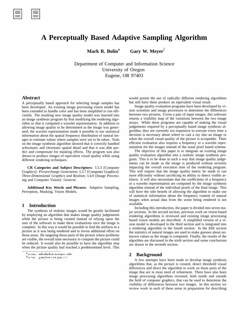
Figure 1: Block diagram of vision model.

the frequency domain in order to perform its filtering operations.The Sarnoff VDM focuses more attention on modeling the phys-iology of the visual pathway. It therefore operates in the spatialdomain and does a careful simulation of such things as the opticalpoint spread function.

In recent work, the Daly VDP and the Sarnoff VDM have beenapplied to precomputed computer graphic imagery. Rushmeier, et.al [25] used the initial stages of the Daly VDP (and other visionmetrics) to compare a simulated and a measured image. Ferwerda,et. al. [7] extended the Daly VDP to include color and modifiedhow it handles masking. The result was a new image processingbased model of the visual system that they used to demonstratehow surface texture can mask polygonal tessellation. Li [15,16]has used computer graphic pictures to compare the Daly VDP andthe Sarnoff VDM. She found that the two models performed com-parably, but that the Sarnoff VDM gave better image differencemaps and required less recalibration. The Sarnoff VDM was alsodetermined to have better execution speed than the Daly VDP butrequired the use of significantly more memory. As a result of thiscomparison we have decided to use the Sarnoff VDM as the basisfor our new vision based rendering algorithm.

3 Simplified Vision ModelThe vision model that we have developed bears many simi-

larities to the Sarnoff VDM discussed in the previous section. Increating a new model of visual perception we were motivated bytwo primary factors. The first and foremost criteria is the speed ofthe visual model. Modern visual difference predictors have goneto great lengths to accurately model the perceptual sensitivity ofthe human visual system. However, efficiency is seldom a designcriteria in developing these systems. This fact limits the utility ofthese algorithms in applications where speed is a primary concern.The second factor that motivated our development of a new modelis the correct handling of color. The majority of visual differencepredictors have been designed only for gray scale images, andthe ones that include color have neglected the significant effect ofchromatic aberration.

The perceptual model that will be described has been imbed-

ded into a visual difference predictor. This difference predictorreceives* as input two images specified in CIE XYZ color space.It returns as output a map of the perceptual difference betweenthe two images specified in terms of just noticeable differences(JND’s). One JND corresponds to a 75% probability that an ob-server viewing the two images would be able to detect a differ-ence, and the units correspond to a roughly linear magnitude ofsubjective visual differences [17].

A block diagram of our visual difference predictor is given inFigure 1. The steps cone fundamentals through spatial poolingare carried out independently on both input images. The differ-ences between the two images are accumulated in the distancesummation step.

In the first stage of the vision model entitled cone fundamen-tals, the pixels of the input image are encoded into the responsesof the short (S), medium (M) and long (L) receptors found in theretina of the eye. This is accomplished using the transformationfrom CIE XYZ to SML space specified by Bolin and Meyer [2].

There is now abundant evidence for the existence of channelsin the visual pathway that are tuned to a number of specific fre-quencies and orientations [17]. The visual processing that occurson a channel is relatively independent of all other channels. Inthe Sarnoff VDM this cortex filtering stage is accomplished bytransforming the image into a Laplacian pyramid and applying aset of oriented filters. The net result is a pyramidal image decom-position that is tuned to seven spatial frequencies and four angulardirections. This transform is the primary source of expense in theSarnoff VDM. In order to reduce the cost of this operation wedecided to model the spatial frequency and orientation selectivityof the visual system through the use of a simple Haar wavelettransform. A number of other wavelet bases were considered, in-cluding Daubechies’ family of wavelets [6] and the biorthogonalbases of Cohen, et. al. [4]. However, these transforms were dis-carded due to their expense. The two-dimensional non-standardHaar decomposition can be expressed as:+�,�-/.1032 4�576498;: <=+�,=0 2 5 6 87>?+�,=0 2 >A@�5 6 87>+",=0 2 5 6 >A@�87>?+�,=0 2 >A@�5 6 >A@"8CB!D�EF .,�-/. 032 4 576 4 8;: <=+�,=0 2 5 6 8�GH+�,=0 2 >A@�5 6 87>+",=0 2 5 6 >A@�8�GH+�,=0 2 >A@�5 6 >A@"8CB!D�EF�I ,�-/. 032 4�576498;: <=+ , 0 2 5 6 87>?+ , 0 2 >A@�5 6 8�G+ , 0 2 5 6 >A@�8�GH+ , 0 2 >A@�5 6 >A@"8CB!D�EF�J ,�-/. 032 4�576498;: <=+ , 0 2 5 6 8�GH+ , 0 2 >A@�5 6 8�G+ , 0 2 5 6 >A@�87>?+ , 0 2 >A@�5 6 >A@"8CB!D�E <!@KBwhere +�, specifies the lowpass coefficients of the level L Haar

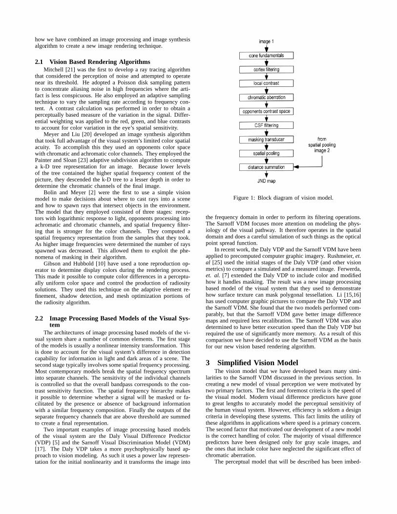
Figure 2: Angular tuning of Haar coefficients.

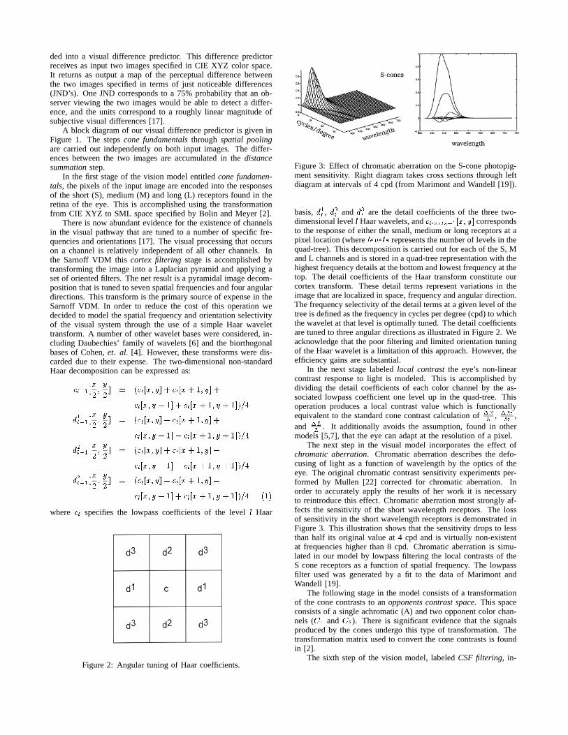
Figure 3: Effect of chromatic aberration on the S-cone photopig-ment sensitivity. Right diagram takes cross sections through leftdiagram at intervals of 4 cpd (from Marimont and Wandell [19]).

basis,F ., , F I , and

F J , are the detail coefficients of the three two-dimensional level L Haar wavelets, and +�,NM�O"M�,QP3-9.10 2 5 6 8 correspondsto the response of either the small, medium or long receptors at apixel location (where L�RKSTRKL�U represents the number of levels in thequad-tree). This decomposition is carried out for each of the S, Mand L channels and is stored in a quad-tree representation with thehighest frequency details at the bottom and lowest frequency at thetop. The detail coefficients of the Haar transform constitute ourcortex transform. These detail terms represent variations in theimage that are localized in space, frequency and angular direction.The frequency selectivity of the detail terms at a given level of thetree is defined as the frequency in cycles per degree (cpd) to whichthe wavelet at that level is optimally tuned. The detail coefficientsare tuned to three angular directions as illustrated in Figure 2. Weacknowledge that the poor filtering and limited orientation tuningof the Haar wavelet is a limitation of this approach. However, theefficiency gains are substantial.

In the next stage labeled local contrast the eye’s non-linearcontrast response to light is modeled. This is accomplished bydividing the detail coefficients of each color channel by the as-sociated lowpass coefficient one level up in the quad-tree. Thisoperation produces a local contrast value which is functionallyequivalent to the standard cone contrast calculation of V�WW , VYXX ,and VYZZ . It additionally avoids the assumption, found in othermodels [5,7], that the eye can adapt at the resolution of a pixel.

The next step in the visual model incorporates the effect ofchromatic aberration. Chromatic aberration describes the defo-cusing of light as a function of wavelength by the optics of theeye. The original chromatic contrast sensitivity experiments per-formed by Mullen [22] corrected for chromatic aberration. Inorder to accurately apply the results of her work it is necessaryto reintroduce this effect. Chromatic aberration most strongly af-fects the sensitivity of the short wavelength receptors. The lossof sensitivity in the short wavelength receptors is demonstrated inFigure 3. This illustration shows that the sensitivity drops to lessthan half its original value at 4 cpd and is virtually non-existentat frequencies higher than 8 cpd. Chromatic aberration is simu-lated in our model by lowpass filtering the local contrasts of theS cone receptors as a function of spatial frequency. The lowpassfilter used was generated by a fit to the data of Marimont andWandell [19].

The following stage in the model consists of a transformationof the cone contrasts to an opponents contrast space. This spaceconsists of a single achromatic (A) and two opponent color chan-nels ( [ . and [ I ). There is significant evidence that the signalsproduced by the cones undergo this type of transformation. Thetransformation matrix used to convert the cone contrasts is foundin [2].

The sixth step of the vision model, labeled CSF filtering, in-

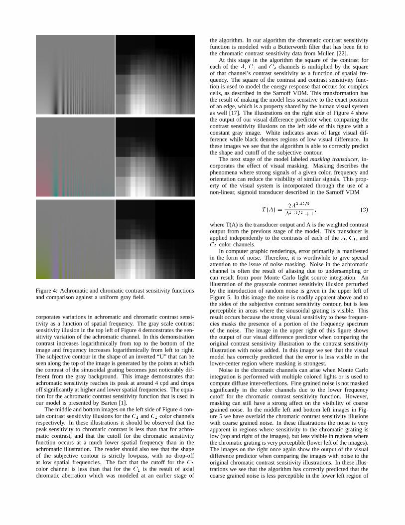
Figure 4: Achromatic and chromatic contrast sensitivity functionsand comparison against a uniform gray field.

corporates variations in achromatic and chromatic contrast sensi-tivity as a function of spatial frequency. The gray scale contrastsensitivity illusion in the top left of Figure 4 demonstrates the sen-sitivity variation of the achromatic channel. In this demonstrationcontrast increases logarithmically from top to the bottom of theimage and frequency increases logarithmically from left to right.The subjective contour in the shape of an inverted “U” that can beseen along the top of the image is generated by the points at whichthe contrast of the sinusoidal grating becomes just noticeably dif-ferent from the gray background. This image demonstrates thatachromatic sensitivity reaches its peak at around 4 cpd and dropsoff significantly at higher and lower spatial frequencies. The equa-tion for the achromatic contrast sensitivity function that is used inour model is presented by Barten [1].

The middle and bottom images on the left side of Figure 4 con-tain contrast sensitivity illusions for the [ . and [ I color channelsrespectively. In these illustrations it should be observed that thepeak sensitivity to chromatic contrast is less than that for achro-matic contrast, and that the cutoff for the chromatic sensitivityfunction occurs at a much lower spatial frequency than in theachromatic illustration. The reader should also see that the shapeof the subjective contour is strictly lowpass, with no drop-offat low spatial frequencies. The fact that the cutoff for the [ Icolor channel is less than that for the [ . is the result of axialchromatic aberration which was modeled at an earlier stage of

the algorithm. In our algorithm the chromatic contrast sensitivityfunction is modeled with a Butterworth filter that has been fit tothe chromatic contrast sensitivity data from Mullen [22].

At this stage in the algorithm the square of the contrast foreach of the \ , [ . and [ I channels is multiplied by the squareof that channel’s contrast sensitivity as a function of spatial fre-quency. The square of the contrast and contrast sensitivity func-tion is used to model the energy response that occurs for complexcells, as described in the Sarnoff VDM. This transformation hasthe result of making the model less sensitive to the exact positionof an edge, which is a property shared by the human visual systemas well [17]. The illustrations on the right side of Figure 4 showthe output of our visual difference predictor when comparing thecontrast sensitivity illusions on the left side of this figure with aconstant gray image. White indicates areas of large visual dif-ference while black denotes regions of low visual difference. Inthese images we see that the algorithm is able to correctly predictthe shape and cutoff of the subjective contour.

The next stage of the model labeled masking transducer, in-corporates the effect of visual masking. Masking describes thephenomena where strong signals of a given color, frequency andorientation can reduce the visibility of similar signals. This prop-erty of the visual system is incorporated through the use of anon-linear, sigmoid transducer described in the Sarnoff VDM

] < \ BY: 4 \ I_^ I!`&a�I\ I&^ b�`_a3I >A@ 5 < 4 Bwhere T(A) is the transducer output and A is the weighted contrastoutput from the previous stage of the model. This transducer isapplied independently to the contrasts of each of the \ , [ . , and[ I color channels.

In computer graphic renderings, error primarily is manifestedin the form of noise. Therefore, it is worthwhile to give specialattention to the issue of noise masking. Noise in the achromaticchannel is often the result of aliasing due to undersampling orcan result from poor Monte Carlo light source integration. Anillustration of the grayscale contrast sensitivity illusion perturbedby the introduction of random noise is given in the upper left ofFigure 5. In this image the noise is readily apparent above and tothe sides of the subjective contrast sensitivity contour, but is lessperceptible in areas where the sinusoidal grating is visible. Thisresult occurs because the strong visual sensitivity to these frequen-cies masks the presence of a portion of the frequency spectrumof the noise. The image in the upper right of this figure showsthe output of our visual difference predictor when comparing theoriginal contrast sensitivity illustration to the contrast sensitivityillustration with noise added. In this image we see that the visualmodel has correctly predicted that the error is less visible in thelower-center region where masking is strongest.

Noise in the chromatic channels can arise when Monte Carlointegration is performed with multiple colored lights or is used tocompute diffuse inter-reflections. Fine grained noise is not maskedsignificantly in the color channels due to the lower frequencycutoff for the chromatic contrast sensitivity function. However,masking can still have a strong affect on the visibility of coarsegrained noise. In the middle left and bottom left images in Fig-ure 5 we have overlaid the chromatic contrast sensitivity illusionswith coarse grained noise. In these illustrations the noise is veryapparent in regions where sensitivity to the chromatic grating islow (top and right of the images), but less visible in regions wherethe chromatic grating is very perceptible (lower left of the images).The images on the right once again show the output of the visualdifference predictor when comparing the images with noise to theoriginal chromatic contrast sensitivity illustrations. In these illus-trations we see that the algorithm has correctly predicted that thecoarse grained noise is less perceptible in the lower left region of

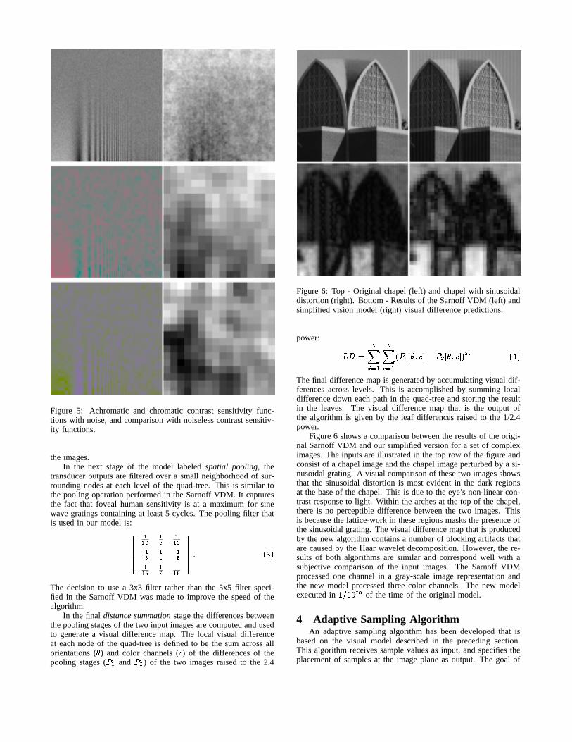
Figure 5: Achromatic and chromatic contrast sensitivity func-tions with noise, and comparison with noiseless contrast sensitiv-ity functions.

the images.In the next stage of the model labeled spatial pooling, the

transducer outputs are filtered over a small neighborhood of sur-rounding nodes at each level of the quad-tree. This is similar tothe pooling operation performed in the Sarnoff VDM. It capturesthe fact that foveal human sensitivity is at a maximum for sinewave gratings containing at least 5 cycles. The pooling filter thatis used in our model is: c

de..3f .g ..3f.g .h .g..3f .g ..3f

ikjlHm <�n�B

The decision to use a 3x3 filter rather than the 5x5 filter speci-fied in the Sarnoff VDM was made to improve the speed of thealgorithm.

In the final distance summation stage the differences betweenthe pooling stages of the two input images are computed and usedto generate a visual difference map. The local visual differenceat each node of the quad-tree is defined to be the sum across allorientations ( o ) and color channels ( + ) of the differences of thepooling stages ( p . and p I ) of the two images raised to the 2.4

Figure 6: Top - Original chapel (left) and chapel with sinusoidaldistortion (right). Bottom - Results of the Sarnoff VDM (left) andsimplified vision model (right) visual difference predictions.

power: qsr : Jt u�v .Jt w�v . < p .10 o 5'+!8�G p I 0 o 5'+!8�B I&^ h <�ETB

The final difference map is generated by accumulating visual dif-ferences across levels. This is accomplished by summing localdifference down each path in the quad-tree and storing the resultin the leaves. The visual difference map that is the output ofthe algorithm is given by the leaf differences raised to the 1/2.4power.

Figure 6 shows a comparison between the results of the origi-nal Sarnoff VDM and our simplified version for a set of compleximages. The inputs are illustrated in the top row of the figure andconsist of a chapel image and the chapel image perturbed by a si-nusoidal grating. A visual comparison of these two images showsthat the sinusoidal distortion is most evident in the dark regionsat the base of the chapel. This is due to the eye’s non-linear con-trast response to light. Within the arches at the top of the chapel,there is no perceptible difference between the two images. Thisis because the lattice-work in these regions masks the presence ofthe sinusoidal grating. The visual difference map that is producedby the new algorithm contains a number of blocking artifacts thatare caused by the Haar wavelet decomposition. However, the re-sults of both algorithms are similar and correspond well with asubjective comparison of the input images. The Sarnoff VDMprocessed one channel in a gray-scale image representation andthe new model processed three color channels. The new modelexecuted in @KD�xzy�{Q| of the time of the original model.

4 Adaptive Sampling AlgorithmAn adaptive sampling algorithm has been developed that is

based on the visual model described in the preceding section.This algorithm receives sample values as input, and specifies theplacement of samples at the image plane as output. The goal of

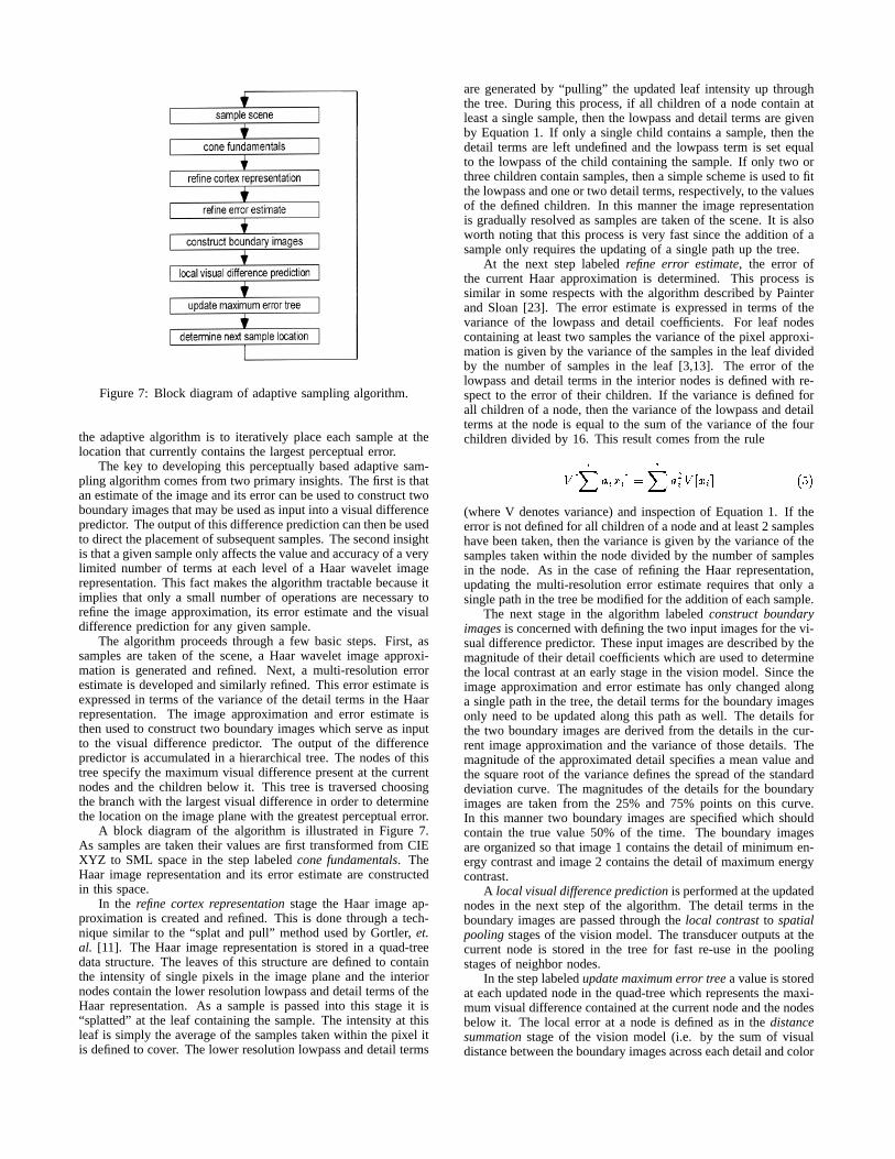
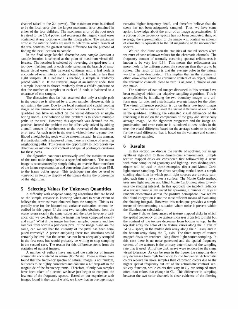
Figure 7: Block diagram of adaptive sampling algorithm.

the adaptive algorithm is to iteratively place each sample at thelocation that currently contains the largest perceptual error.

The key to developing this perceptually based adaptive sam-pling algorithm comes from two primary insights. The first is thatan estimate of the image and its error can be used to construct twoboundary images that may be used as input into a visual differencepredictor. The output of this difference prediction can then be usedto direct the placement of subsequent samples. The second insightis that a given sample only affects the value and accuracy of a verylimited number of terms at each level of a Haar wavelet imagerepresentation. This fact makes the algorithm tractable because itimplies that only a small number of operations are necessary torefine the image approximation, its error estimate and the visualdifference prediction for any given sample.

The algorithm proceeds through a few basic steps. First, assamples are taken of the scene, a Haar wavelet image approxi-mation is generated and refined. Next, a multi-resolution errorestimate is developed and similarly refined. This error estimate isexpressed in terms of the variance of the detail terms in the Haarrepresentation. The image approximation and error estimate isthen used to construct two boundary images which serve as inputto the visual difference predictor. The output of the differencepredictor is accumulated in a hierarchical tree. The nodes of thistree specify the maximum visual difference present at the currentnodes and the children below it. This tree is traversed choosingthe branch with the largest visual difference in order to determinethe location on the image plane with the greatest perceptual error.

A block diagram of the algorithm is illustrated in Figure 7.As samples are taken their values are first transformed from CIEXYZ to SML space in the step labeled cone fundamentals. TheHaar image representation and its error estimate are constructedin this space.

In the refine cortex representation stage the Haar image ap-proximation is created and refined. This is done through a tech-nique similar to the “splat and pull” method used by Gortler, et.al. [11]. The Haar image representation is stored in a quad-treedata structure. The leaves of this structure are defined to containthe intensity of single pixels in the image plane and the interiornodes contain the lower resolution lowpass and detail terms of theHaar representation. As a sample is passed into this stage it is“splatted” at the leaf containing the sample. The intensity at thisleaf is simply the average of the samples taken within the pixel itis defined to cover. The lower resolution lowpass and detail terms

are generated by “pulling” the updated leaf intensity up throughthe tree. During this process, if all children of a node contain atleast a single sample, then the lowpass and detail terms are givenby Equation 1. If only a single child contains a sample, then thedetail terms are left undefined and the lowpass term is set equalto the lowpass of the child containing the sample. If only two orthree children contain samples, then a simple scheme is used to fitthe lowpass and one or two detail terms, respectively, to the valuesof the defined children. In this manner the image representationis gradually resolved as samples are taken of the scene. It is alsoworth noting that this process is very fast since the addition of asample only requires the updating of a single path up the tree.

At the next step labeled refine error estimate, the error ofthe current Haar approximation is determined. This process issimilar in some respects with the algorithm described by Painterand Sloan [23]. The error estimate is expressed in terms of thevariance of the lowpass and detail coefficients. For leaf nodescontaining at least two samples the variance of the pixel approxi-mation is given by the variance of the samples in the leaf dividedby the number of samples in the leaf [3,13]. The error of thelowpass and detail terms in the interior nodes is defined with re-spect to the error of their children. If the variance is defined forall children of a node, then the variance of the lowpass and detailterms at the node is equal to the sum of the variance of the fourchildren divided by 16. This result comes from the rule

} 0�~t �~ 2 ~ 89: ~t � I ~ } 0 2 ~ 8 <���B

(where V denotes variance) and inspection of Equation 1. If theerror is not defined for all children of a node and at least 2 sampleshave been taken, then the variance is given by the variance of thesamples taken within the node divided by the number of samplesin the node. As in the case of refining the Haar representation,updating the multi-resolution error estimate requires that only asingle path in the tree be modified for the addition of each sample.

The next stage in the algorithm labeled construct boundaryimages is concerned with defining the two input images for the vi-sual difference predictor. These input images are described by themagnitude of their detail coefficients which are used to determinethe local contrast at an early stage in the vision model. Since theimage approximation and error estimate has only changed alonga single path in the tree, the detail terms for the boundary imagesonly need to be updated along this path as well. The details forthe two boundary images are derived from the details in the cur-rent image approximation and the variance of those details. Themagnitude of the approximated detail specifies a mean value andthe square root of the variance defines the spread of the standarddeviation curve. The magnitudes of the details for the boundaryimages are taken from the 25% and 75% points on this curve.In this manner two boundary images are specified which shouldcontain the true value 50% of the time. The boundary imagesare organized so that image 1 contains the detail of minimum en-ergy contrast and image 2 contains the detail of maximum energycontrast.

A local visual difference prediction is performed at the updatednodes in the next step of the algorithm. The detail terms in theboundary images are passed through the local contrast to spatialpooling stages of the vision model. The transducer outputs at thecurrent node is stored in the tree for fast re-use in the poolingstages of neighbor nodes.

In the step labeled update maximum error tree a value is storedat each updated node in the quad-tree which represents the maxi-mum visual difference contained at the current node and the nodesbelow it. The local error at a node is defined as in the distancesummation stage of the vision model (i.e. by the sum of visualdistance between the boundary images across each detail and color

channel raised to the 2.4 power). The maximum error is definedto be the local error plus the largest maximum error contained ineither of the four children. The maximum error of the root nodeis raised to the 1/2.4 power and represents the largest visual errorcontained at any location within the image plane. The maximumerror in the interior nodes are used to determine which branch ofthe tree contains the greatest visual difference for the purpose offinding the next location to sample.

In the final stage labeled determine next sample location asample location is selected at the point of maximum visual dif-ference. The location is selected by traversing the quad-tree in atop-down fashion and, at each node, selecting the branch of max-imum visual error. This traversal continues until a leaf node isencountered or an interior node is found which contains less thaneight samples. If a leaf node is reached, a sample is randomlyplaced within it. If the traversal stops at an interior node, thena sample location is chosen randomly from a child’s quadrant sothat the number of samples in each child node is balanced to atolerance of one sample.

The discussion thus far has assumed that only a single pathin the quad-tree is affected by a given sample. However, this isnot strictly the case. Due to the local contrast and spatial poolingstages of the vision model the modification of one node in thequad-tree can have an affect on the visual difference at neigh-boring nodes. One solution to this problem is to update multiplepaths up the tree. However, this approach was deemed too ex-pensive. Instead the problem can be effectively solved by addinga small amount of randomness to the traversal of the maximumerror tree. As each node in the tree is visited, there is some like-lihood a neighboring node will be chosen instead. In this manner,if a particular path is traversed often, there is a chance of selectingneighboring paths. This creates the opportunity to incorporate up-dated values into the local contrast and spatial pooling calculationsfor these paths.

The algorithm continues recursively until the maximum errorof the root node drops below a specified tolerance. The outputimage is reconstructed by simply doing an inverse Haar transformof the image representation and converting pixel values from SMLto the frame buffer space. This technique can also be used toconstruct an iterative display of the image during the progressionof the algorithm.

5 Selecting Values for Unknown QuantitiesA difficulty with adaptive sampling algorithms that are based

on the sample variance is knowing when and to what extent tobelieve the error estimate obtained from the samples. This is es-pecially true for the hierarchical variance estimation scheme de-scribed in this paper. If the first two samples obtained from thescene return exactly the same values and therefore have zero vari-ance, can we conclude that the image has been computed exactlyand stop? What if the image has been sampled densely and twosamples from within a particular pixel of the image plane are thesame, can we say that the intensity of the pixel has been com-puted correctly? A person analyzing these two situations wouldcertainly believe that the scene has not been adequately sampledin the first case, but would probably be willing to stop samplingin the second case. The reason for this difference stems from thestatistics of natural images.

A number of authors have analyzed the statistics of imagescommonly encountered in nature [8,9,24,26]. These authors havefound that the frequency spectra of natural images is not random,but tends to be highly correlated and contains a 1/f drop-off in themagnitude of the frequency terms. Therefore, if only two sampleshave been taken of a scene, we have just begun to compute thelow end of the frequency spectra. Based on our experience withimages found in the natural world, we know that an average image

contains higher frequency detail, and therefore believe that thescene has not been adequately sampled. Thus, we have someapriori knowledge about the error of an image approximation. Ifa portion of the frequency spectra has not been computed, then, onaverage, the approximation of the image will contain an amountof error that is equivalent to the 1/f magnitude of the uncomputedspectra.

We can also draw upon the statistics of natural scenes whenwe must choose unknown values for the chromatic channels. Thefrequency content of naturally occurring spectral reflectances isknown to be very low [18]. This means that reflectances aremore likely to be uniform across the spectrum than they are to bespikey. The result of this is that the average color in the naturalworld is quite desaturated. This implies that in the absence ofother knowledge about the chromatic content of an object, settingthe chromatic channels close to zero is as good a choice as onecan make.

The statistics of natural images discussed in this section havebeen employed within our adaptive sampling algorithm. This isaccomplished by initializing the two boundary images to a uni-form gray for one, and a statistically average image for the other.The visual difference predictor is run on these two input imagesand the output is used to seed the visual difference at each nodein the quad-tree. Initially, the estimated visual difference of therendering is based on the comparison of the gray and statisticallyaverage image. As the algorithm progresses and the image ap-proximation and error estimate is calculated at new nodes in thetree, the visual difference based on the average statistics is tradedfor the visual difference that is based on the variance and contentof the scene samples.

6 ResultsIn this section we discuss the results of applying our image

synthesis algorithm to three dimensional environments. Simpletexture mapped disks are considered first followed by a scenewith more complicated geometry and lighting. Two shading tech-niques will be used in these examples, direct and Monte Carlolight source sampling. The direct sampling method uses a simpleshading algorithm in which point light sources are directly sam-pled each time a ray strikes a surface. The Monte Carlo methoduses area light sources and blind Monte Carlo integration to eval-uate the shading integral. In this approach the incident radianceat a surface point is evaluated by spawning a number of rays atrandom orientations across the positive hemisphere. We realizethat blind integration is not the most efficient means of evaluatingthe shading integral. However, this technique provides a simplemeans of demonstrating a situation where noise is present withinthe illumination calculation.

Figure 8 shows three arrays of texture mapped disks in whichthe spatial frequency of the texture increases from left to right butthe contrast of the texture decreases from bottom to top. In thetop disk array the color of the texture varies along the \ axis of\�[ . [ I space, in the middle disk array along the [ . axis, and inthe bottom array along the [ I axis. The three arrays of texturemapped disks are rendered using direct light source sampling. Inthis case there is no noise generated and the spatial frequencycontent of the textures is the primary determinant of the samplingrate that is used. All of the disk arrays were rendered to the samevisual tolerance. As can be seen in the figure, the sampling den-sity decreases from high frequency to low frequency. Achromaticcolors receive far more samples than chromatic colors due to thehigher spatial frequency cut off of the achromatic contrast sen-sitivity function, while colors that vary in [ . are sampled moreoften than colors that change in [ I . This difference in samplingbetween the two color channels is clear evidence of the filtering

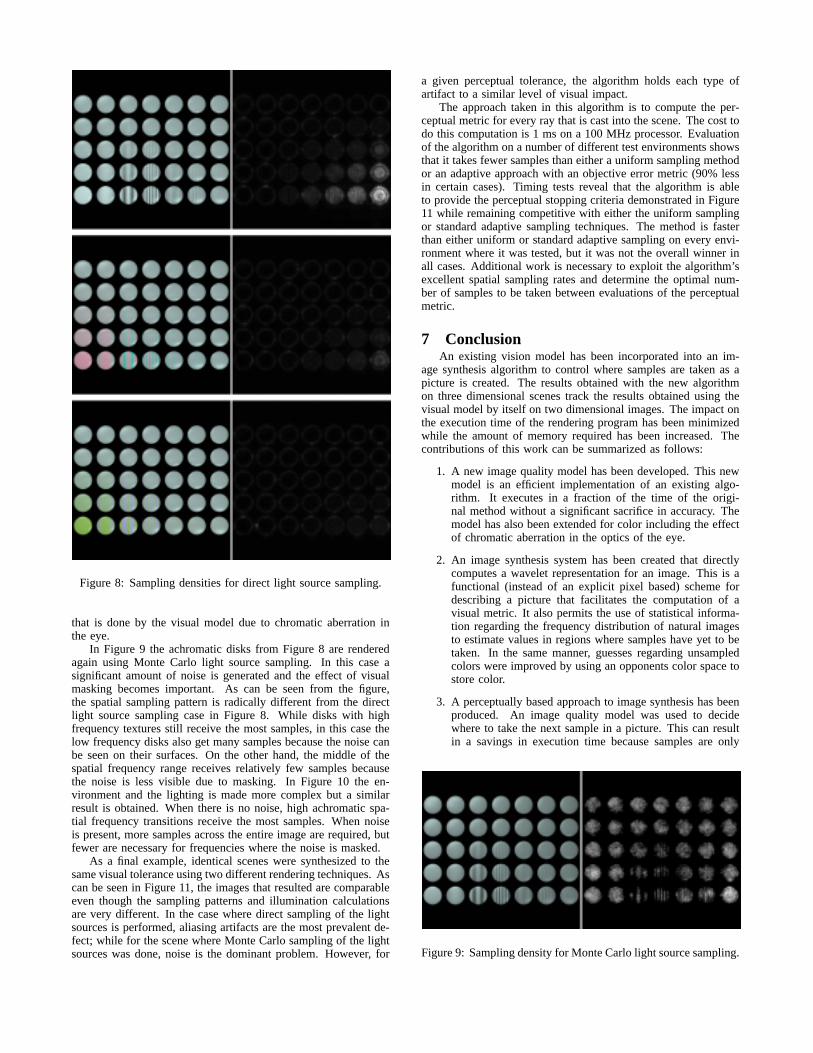
Figure 8: Sampling densities for direct light source sampling.

that is done by the visual model due to chromatic aberration inthe eye.

In Figure 9 the achromatic disks from Figure 8 are renderedagain using Monte Carlo light source sampling. In this case asignificant amount of noise is generated and the effect of visualmasking becomes important. As can be seen from the figure,the spatial sampling pattern is radically different from the directlight source sampling case in Figure 8. While disks with highfrequency textures still receive the most samples, in this case thelow frequency disks also get many samples because the noise canbe seen on their surfaces. On the other hand, the middle of thespatial frequency range receives relatively few samples becausethe noise is less visible due to masking. In Figure 10 the en-vironment and the lighting is made more complex but a similarresult is obtained. When there is no noise, high achromatic spa-tial frequency transitions receive the most samples. When noiseis present, more samples across the entire image are required, butfewer are necessary for frequencies where the noise is masked.

As a final example, identical scenes were synthesized to thesame visual tolerance using two different rendering techniques. Ascan be seen in Figure 11, the images that resulted are comparableeven though the sampling patterns and illumination calculationsare very different. In the case where direct sampling of the lightsources is performed, aliasing artifacts are the most prevalent de-fect; while for the scene where Monte Carlo sampling of the lightsources was done, noise is the dominant problem. However, for

a given perceptual tolerance, the algorithm holds each type ofartifact to a similar level of visual impact.

The approach taken in this algorithm is to compute the per-ceptual metric for every ray that is cast into the scene. The cost todo this computation is 1 ms on a 100 MHz processor. Evaluationof the algorithm on a number of different test environments showsthat it takes fewer samples than either a uniform sampling methodor an adaptive approach with an objective error metric (90% lessin certain cases). Timing tests reveal that the algorithm is ableto provide the perceptual stopping criteria demonstrated in Figure11 while remaining competitive with either the uniform samplingor standard adaptive sampling techniques. The method is fasterthan either uniform or standard adaptive sampling on every envi-ronment where it was tested, but it was not the overall winner inall cases. Additional work is necessary to exploit the algorithm’sexcellent spatial sampling rates and determine the optimal num-ber of samples to be taken between evaluations of the perceptualmetric.

7 ConclusionAn existing vision model has been incorporated into an im-

age synthesis algorithm to control where samples are taken as apicture is created. The results obtained with the new algorithmon three dimensional scenes track the results obtained using thevisual model by itself on two dimensional images. The impact onthe execution time of the rendering program has been minimizedwhile the amount of memory required has been increased. Thecontributions of this work can be summarized as follows:

1. A new image quality model has been developed. This newmodel is an efficient implementation of an existing algo-rithm. It executes in a fraction of the time of the origi-nal method without a significant sacrifice in accuracy. Themodel has also been extended for color including the effectof chromatic aberration in the optics of the eye.

2. An image synthesis system has been created that directlycomputes a wavelet representation for an image. This is afunctional (instead of an explicit pixel based) scheme fordescribing a picture that facilitates the computation of avisual metric. It also permits the use of statistical informa-tion regarding the frequency distribution of natural imagesto estimate values in regions where samples have yet to betaken. In the same manner, guesses regarding unsampledcolors were improved by using an opponents color space tostore color.

3. A perceptually based approach to image synthesis has beenproduced. An image quality model was used to decidewhere to take the next sample in a picture. This can resultin a savings in execution time because samples are only

Figure 9: Sampling density for Monte Carlo light source sampling.

Figure 10: Sampling densities for direct (left) and Monte Carlo (right) light source sampling. Color varies in the middle three rows alongthe [ I , [ . , and \ axes of \�[ . [ I space. Contrast of the middle three balls in the [ I and \ rows is decreased in the top two and bottomtwo rows respectively.

taken in areas where there are visible artifacts. The imagequality model is also used to decide when enough sampleshave been taken across the entire image. This provides avisual stopping condition and makes it possible to employdifferent rendering algorithms but still produce equivalentpictures.

This work represents a first attempt to imbed a sophisticatedimage processing vision model into an image synthesis algorithm.While the results are encouraging it is clear that the approachtaken here puts a certain amount of overhead onto every ray thatis cast into the scene. An alternative tactic might be to initiallysample the image at a low rate and compute the visual differencemap from these values. The visual difference map can then beused to select regions of the image which require further sampling.The use of the imbedded version of the vision model might besaved until the image is more fully developed and the maskingeffects have become completely apparent.

8 AcknowledgementsThe authors would like to thank Jae H. Kim for his help in

creating Figures 8, 9, 10, and 11 and for his assistance in as-sembling all of the color figures in this paper. This research wasfunded by the National Science Foundation under grant numberCCR 96-19967.

9 References[1] Barten, P. G. J., “The Square Root Integral (SQRI): A New Metric

to Describe the Effect of Various Display Parameters on PerceivedImage Quality,” Human Vision, Visual Processing, and DigitalDisplay, Proc. SPIE, Vol. 1077, pp. 73-82, 1989.

[2] Bolin, M. R. and Meyer G. W., “A Frequency Based Ray Tracer,”Computer Graphics, Annual Conference Series, ACM SIG-GRAPH, pp. 409-418, 1995.

[3] Bolin, M. R. and Meyer G. W., “An Error Metric for Monte Carlo RayTracing,” Rendering Techniques ’97, J. Dorsey and P. Slusallek,Editors, Springer-Verlag, New York, pp. 57-68, 1997.

[4] Cohen, A., Daubechies, I., and Feauveau, J. C., “Biorthogonal Basesof Compactly Supported Wavelets,” Communications on Pure andApplied Mathematics, Vol. 45, No. 5, pp. 485-500, 1992.

[5] Daly, S., “The Visible Differences Predictor: An Algorithm for theAssessment of Image Fidelity,” Digital Images and Human Vision,A. B. Watson, Editor, MIT Press, Cambridge, MA, pp. 179-206, 1993.

[6] Daubechies, I., “Orthonormal Bases of Compactly SupportedWavelets,” Communications on Pure and Applied Mathemat-ics, Vol. 41, No. 7, pp. 909-996, 1988.

[7] Ferwerda, J. A., Shirley, P., Pattanaik, S. N., and Greenberg, D. P.,“A Model of Visual Masking for Computer Graphics,” ComputerGraphics, Annual Conference Series, ACM SIGGRAPH, pp. 143-152, 1997.

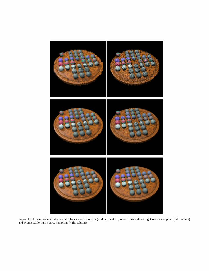
Figure 11: Image rendered at a visual tolerance of 7 (top), 5 (middle), and 3 (bottom) using direct light source sampling (left column)and Monte Carlo light source sampling (right column).

[8] Field, D. J., “Relations Between the Statistics of Natural Images andthe� Response Properties of Cortical Cells,” J. Opt. Soc. Am. A, Vol.4, pp. 2379-2394, 1987.

[9] Field, D. J., “What the Statistics of Natural Images Tell Us AboutVisual Coding,” Human Vision, Visual Processing, and DigitalDisplay, Proc. SPIE, Vol. 1077, pp. 269-276, 1989.

[10] Gibson, S. and Hubbold, R. J., “Perceptually-Driven Radiosity,”Computer Graphics Forum, Vol. 16, pp. 129-140, 1997.

[11] Gortler, S. J., Grzeszczuk, R., Szeliski, R., and Cohen, M. F., “TheLumigraph,” Computer Graphics, Annual Conference Series,ACM SIGGRAPH, pp. 43-54, 1996.

[12] Kirk, D. and Arvo, J., “Unbiased Sampling Techniques for Im-age Synthesis,” Computer Graphics, Annual Conference Series,ACM SIGGRAPH, pp. 153-156, 1991.

[13] Lee, M. E., Redner, R. A., and Uselton, S. P., “Statistically Opti-mized Sampling for Distributed Ray Tracing,” Computer Graphics,Annual Conference Series, ACM SIGGRAPH, pp. 61-67, 1985.

[14] Legge, G. E. and Foley, J. M., “Contrast Masking in human vision,”Journal of the Optical Society of America, Vol. 70, pp. 1458-1470, 1980.

[15] Li, B., “An Analysis and Comparison of Two Visual DiscriminationModels,” Master’s Thesis, University of Oregon, June 1997.

[16] Li, B., Meyer, G. W., and Klassen, R. V., “A Comparison of TwoImage Quality Models,” to appear in Human Vision and ElectronicImaging III, B. E. Rogowitz and T. N. Pappas, Editors, Proc. SPIE,Vol. 3299, 1998.

[17] Lubin, J., “A Visual Discrimination Model for Imaging System De-sign and Evaluation,” Vision Models for Target Detection andRecognition, Eli Peli, Editor, World Scientific, New Jersey, pp. 245-283, 1995.

[18] Maloney, L. T., “Evaluation of linear models of surface spectralreflectance with small numbers of parameters,” J. Opt. Soc. Am. A,Vol. 3, pp. 1673-1683. 1986.

[19] Marimont, D. H. and Wandell, B. A., “Matching Color Images: TheImpact of Axial Chromatic Aberration,” J. Opt. Soc. Am. A, Vol.12, pp. 3113-3122, 1993.

[20] Meyer, G. W. and Liu, A., “Color Spatial Acuity Control of a ScreenSubdivision Image Synthesis Algorithm,” Human Vision, VisualProcessing, and Digital Display III, Bernice E. Rogowitz, Editor,Proc. SPIE, Vol. 1666, pp. 387-399, 1992.

[21] Mitchell, D. P., “Generating Antialiased Images at Low SamplingDensities,” Computer Graphics, Annual Conference Series,ACM SIGGRAPH, pp. 65-72, 1987.

[22] Mullen, K. T., “The Contrast Sensitivity of Human Colour Visionto Red-Green and Blue-Yellow Chromatic Gratings,” J. Physiol.(Lond.), Vol. 359, pp. 381-400, 1985.

[23] Painter, J. and Sloan, K. “Antialiased Ray Tracing by Adaptive Pro-gressive Refinement,” Computer Graphics, Annual ConferenceSeries, ACM SIGGRAPH, pp. 281-288, 1989.

[24] Ruderman, D. L., “Origins of Scaling in Natural Images,” HumanVision, Visual Processing, and Digital Display, Proc. SPIE, Vol.2657, pp. 120-131, 1996.

[25] Rushmeier, H., Ward, G., Piatko, C., Sanders, P., and Rust, B.,“Comparing Real and Synthetic Images: Some Ideas About Metrics,”Rendering Techniques ’95, P. M. Hanrahan and W. Purgathofer,Editors Springer-Verlag, New York, pp. 82-91, 1995.

[26] Schreiber, W. F., Fundamentals of Electronic Imaging Systems,Springer-Verlag: Berlin Heidelberg, 1993.