a perceptually accurate model of the hand
TRANSCRIPT
A Perceptually Accurate Model of the Hand
by
Ye Lu
B. A.Sc. (Computing Science) Simon Fraser University, 1995
A THESIS SUBMITTED IN PARTIAL FULFILLMENT
O F THE REQUIREMENTS FOR THE DEGREE O F
MASTER OF APPLIED SCIENCE
in the School
of
Engineering Science
@ Ye Lu 1997
SIMON FRASER UNIVERSITY
July 1997
All rights reserved. This work may not be
reproduced in whole or in part, by photocopy
or other means, without the permission of the author.

APPROVAL
Name: Ye Lu
Degree: Master of Applied Science
Title of Thesis: A Perceptually Accurate Model of the Hand
Examining Committee: Dr. Kamal Gupta, Associate Professor
Chair
DL John C. Dill, Professor
Senior Supervisor
Dr. Tom W. Calvert, Prafessor
Supervisor
Dr. Ze-Nian Li, Associate Professor
School of Computing Science .
External Examiner
Date Approved: ~ u l y 25 , 1997

PARTIAL COPYRIGHT LICENSE
I hereby grant to Simon Fraser University the right to lend my thesis, project or extended essay (the title of which is shown below) to users of the Simon Fraser University Library, and to make partial or single copies only for such users or in response to a request from the library of any other university, or other educational institution, on its own behalf or for one of its users. I further agree that permission for multiple copying of this work for scholarly purposes may be granted by me or the Dean of Graduate Studies. It is understood that copying or publication of this work for financial gain shall not be allowed without my written permission.
Title of ThesidProjectlExtended Essay
"A Perceptually Accurate Model of the Hand"
Author: (signature)
u (name)
July. 1997 (date)
Abstract
The human hand is used in virtually all aspects of everyday activities involving such
tasks as selection, manipulation and communication. It is therefore important to
study and understand how it works. However, a significant difficulty facing traditional
hand researchers is acquiring accurate 3D data that describes actual human hand
movements. To address this problem, a multidisciplinary team of researchers from
kinesiology, computer science and engineering was formed to design and implement
a Virtual Hand Laboratory to serve as a testbed for future studies of goal-directed
human hand movements.
The primary objective of the work described in this thesis is to provide a framework
for the collection, estimation and display of hand postures from live 3D data. A fast
lookup table-based inverse kinematic algorithm was developed and used to estimate
hand postures from real-time 3D data supplied by the Optotrak system, a powerful
motion capture device.
The algorithm is executed in two stages: a calibration stage and a run-time stage.
The former measures the characteristics of the subject's hand in order to customize
the lookup table while the latter uses the table to estimate the subject's hand posture.
A polygonal model of the human hand was developed for display of the estimated hand
posture. A complete system integrating data collection with estimation and display
of hand postures in real-time was designed and implemented to serve as the platform
for real-time experiments in the study of goal-directed hand movements.

Dedication
To My Parents

Acknowledgments
I would like to thank my senior supervisor Dr. John C. Dill for his invaluable guidance,
enthusiasm and financial support throughout the course of this work. I am also very
grateful to my supervisor Dr. Tom Calvert for his helpful comments and insightful
suggestions during the research and writing of this thesis. I would also like to thank
Dr. Ze-Nian Li for taking the time t o be my external examiner.
Many other people have helped and contributed their time to the research of this
thesis. My thanks to Dr. Kellogg S. Booth and Jason Harrison of the University of
British Columbia for their invaluable comments. Thanks to Sidi Yu for his efforts in
the development of the polygonal model of the hand. Thanks to Dr. Kenji Amaya for
his inspiration and development of the initial algorithm. Thanks to Dr. Hongsheng
Chin for his mathematical expertise as well as his friendship. Thanks t o Wan Gong
for proofreading the draft of this thesis.
I would also like to take this opportunity to express my gratitutes toward everyone
in the Human Motor Systems Laboratory of the School of Kinesiology at Simon Fraser
University, especially Dr. Christine MacKenzie, Dr. Evan Graham, Yanqing Wang,
Beth Brown and Chris Ivens for their valuable suggestions and help in setting up the
equipments for the experiment.
Last but certainly not least, I will always be indebted to my parents, Xiqi Lu and
Taiqiong Ma, and my brother Joe Lu, for their support and confidence in me. This
thesis would not have been possible without their kindness and encouragement.
This research is supported in part by the NSERC Strategic Grant.

Contents
Approval . . . . . . . . . . . . . . . . . . . . . . . . . . . . . . . . . . . . . Abstract . . . . . . . . . . . . . . . . . . . . . . . . . . . . . . . . . . . . . Dedication . . . . . . . . . . . . . . . . . . . . . . . . . . . . . . . . . . . . Acknowledgments . . . . . . . . . . . . . . . . . . . . . . . . . . . . . . . . List of Figures . . . . . . . . . . . . . . . . . . . . . . . . . . . . . . . . . . 1 Introduction . . . . . . . . . . . . . . . . . . . . . . . . . . . . . . . .
. . . . . . . . . . . . . . . . . . . . . . . . . . . . . 1.1 Motivation
1.2 The Inverse Kinematics Approach for Hand Posture Estimation
1.3 Organization of Thesis . . . . . . . . . . . . . . . . . . . . . . 2 Hand Kinematics . . . . . . . . . . . . . . . . . . . . . . . . . . . . .
2.1 Kinematic Methods . . . . . . . . . . . . . . . . . . . . . . . . 2.1.1 Link Description . . . . . . . . . . . . . . . . . . . . 2.1.2 Forward Kinematics . . . . . . . . . . . . . . . . . . 2.1.3 Inverse Kinematics . . . . . . . . . . . . . . . . . . .
2.2 Hand Model . . . . . . . . . . . . . . . . . . . . . . . . . . . . 2.2.1 Human Hand Anatomy . . . . . . . . . . . . . . . . 2.2.2 Internal Skeletal Model . . . . . . . . . . . . . . . . 2.2.3 Polygonal Hand Model . . . . . . . . . . . . . . . . .
3 Inverse Kinematics . . . . . . . . . . . . . . . . . . . . . . . . . . . . 3.1 Problem Definition . . . . . . . . . . . . . . . . . . . . . . . .
. . . . . . . . . . . . . . . . . . 3.1.1 Existence of Solution
3.1.2 Redundancy . . . . . . . . . . . . . . . . . . . . . . . 3.2 Jacobian Based Methods . . . . . . . . . . . . . . . . . . . . .
3.2.1 Inverse and Pseudoinverse of Jacobian . . . . . . . . 19
3.2.2 Singularities . . . . . . . . . . . . . . . . . . . . . . . 19
3.2.3 Homogeneous Solution . . . . . . . . . . . . . . . . . 21
3.2.4 The Jacobian Transpose Method . . . . . . . . . . . 21
3.3 Optimization Based Methods . . . . . . . . . . . . . . . . . . 23
3.4 Table Based Method . . . . . . . . . . . . . . . . . . . . . . . 25
3.4.1 Preprocessing Stage . . . . . . . . . . . . . . . . . . 26
3.4.2 RunTimeStage . . . . . . . . . . . . . . . . . . . . 31
3.4.3 Discussion . . . . . . . . . . . . . . . . . . . . . . . . 34
. . . . . . . . . . . . . . . . . . . . . . . . . . . . . 3.5 Summary 35
4 A Table Based Real-time Algorithm . . . . . . . . . . . . . . . . . . . 37
4.1 Motivation . . . . . . . . . . . . . . . . . . . . . . . . . . . . . 37
4.2 IRED Placements . . . . . . . . . . . . . . . . . . . . . . . . . 40
4.2.1 IRED positions . . . . . . . . . . . . . . . . . . . . . 40
4.3 Hand Posture Estimation . . . . . . . . . . . . . . . . . . . . 42
4.3.1 The Proposed Hand Model . . . . . . . . . . . . . . 43
4.3.2 The Algorithm . . . . . . . . . . . . . . . . . . . . . 51
4.4 Implementation . . . . . . . . . . . . . . . . . . . . . . . . . . 54
4.4.1 The Data Collection System . . . . . . . . . . . . . . 54
. . . . . . . . . . . . . . . . . . . . . . . . . . . . . 4.5 Discussion 5.5
5 Experiment and Results . . . . . . . . . . . . . . . . . . . . . . . . . 58
5.1 The Real-time Experiment . . . . . . . . . . . . . . . . . . . . 58
5.2 Difficulties Encountered . . . . . . . . . . . . . . . . . . . . . 60
5.3 Result and Analysis . . . . . . . . . . . . . . . . . . . . . . . . 67
5.3.1 The Index Finger . . . . . . . . . . . . . . . . . . . . 67
. . . . . . . . . . . . . . . . . . . . . . . 5.3.2 The Thumb 68
. . . . . . . . . . . . . . . . . . . . . . . . . . . . . 5.4 Summary 74
. . . . . . . . . . . . . . . . . . . . . . . . . . . . . . . . 6 Conclusions 75
6.1 Summary . . . . . . . . . . . . . . . . . . . . . . . . . . . . . 76
. . . . . . . . . . . . . . . . . . . . . . . . . . . . 6.2 Future Work 77
. . . . . . . . . . . . . . . . . . . . . . . . . . . . . . . . . . Appendix: A 78
vii

Appendix: B . . . . . . . . . . . . . . . . . . . . . . . . . . . . . . . . . . 79
. . . . . . . . . . . . . . . . . . . . . . . . . . . . . . . . . . Appendix: C S1
. . . . . . . . . . . . . . . . . . . . . . . . . . . . . . . . . . Bibliography S7

List of Figures
2.1 The link parameters . . . . . . . . . . . . . . . . . . . . . . . . . . . 2.2 Anatomy of the human hand . . . . . . . . . . . . . . . . . . . . . . . 2.3 Internal Skeletal Model . . . . . . . . . . . . . . . . . . . . . . . . . . 2.4 Attachment of vertices onto the bone segments . . . . . . . . . . . . . 2.5 Finger bending . . . . . . . . . . . . . . . . . . . . . . . . . . . . . .
3.1 Possible solutions to reach point B . . . . . . . . . . . . . . . . . . . 3.2 IRED placement in the preprocessing stage of Amaya's algorithm . . . 3.3 The hand and fingertip coordinate systems . . . . . . . . . . . . . . . 3.4 The lookup table in Amaya's Algorithm . . . . . . . . . . . . . . . . 3.5 IRED placement at run time . . . . . . . . . . . . . . . . . . . . . . . 3.6 The known and unknown vectors when estimating the orientation and
position of the fingertip . . . . . . . . . . . . . . . . . . . . . . . . . .
4.1 Distance between the finger tip and the MCP joint . . . . . . . . . . . 4.2 Various cases that an IRED could become invisible to the Optotrak
camera . . . . . . . . . . . . . . . . . . . . . . . . . . . . . . . . . . . 4.3 IRED placement for measuring segment lengths . . . . . . . . . . . . . 4.4 IRED placement for real-time experiment . . . . . . . . . . . . . . . . 4.5 A circular joint . . . . . . . . . . . . . . . . . . . . . . . . . . . . . . 4.6 The five link representation of a finger . . . . . . . . . . . . . . . . . 4.7 Calculation of 4; . . . . . . . . . . . . . . . . . . . . . . . . . . . . . 4.8 Calculation of 6$dex . . . . . . . . . . . . . . . . . . . . . . . . . . . . 4.9 Calculation of OYdex . . . . . . . . . . . . . . . . . . . . . . . . . . . .

4.10 Calculation of Ohhumb . . . . . . . . . . . . . . . . . . . . . . . . . . . 4.1 1 Calculation of 04humb . . . . . . . . . . . . . . . . . . . . . . . . . . . 4.12 Calculation of Oihumb . . . . . . . . . . . . . . . . . . . . . . . . . . . 4.13 The lookup table build using the algorithm described in the thesis . . 4.14 Display of collected data . . . . . . . . . . . . . . . . . . . . . . . . .
5-1 Equipmeatsetup . . . . . . . . . . . . . . . . . . . . . . . . . . . . . 5.2 Comparison of O F d e x . . . . . . . . . . . . . . . . . . . . . . . . . . . 5.3 Comparison of 09dex . . . . . . . . . . . . . . . . . . . . . . . . . . . 5.4 Comparison of Of"dex . . . . . . . . . . . . . . . . . . . . . . . . . . . 5.5 Comparison of the x coordinate of the tip of the index finger . . . . . 5.6 Comparison of the y coordinate of the tip of the index finger . . . . . 5.7 The error between measured tip location and computed tip location of
the index finger . . . . . . . . . . . . . . . . . . . . . . . . . . . . . . 5.8 Comparison of Oihumb . . . . . . . . . . . . . . . . . . . . . . . . . . . 5.9 Comparison of OihUmb . . . . . . . . . . . . . . . . . . . . . . . . . . . 5.10 Comparison of the x coordinate of the tip of the thumb . . . . . . . . 5.11 Comparison of the y coordinate of the tip of the thumb . . . . . . . . 5.12 The error between measured tip location and computed tip location of
the thumb . . . . . . . . . . . . . . . . . . . . . . . . . . . . . . . . .

Chapter 1
Introduction
People use their hands for many everyday activities involving such tasks as selection,
manipulation and communication. It is therefore important to study and under-
stand how it works. Accordingly, the study and analysis of goal-directed human hand
movement has become an increasingly important topic in the field of human-computer
interaction (HCI). With the advent of 3D virtual reality systems, gestural input and
full hand pointing are being explored as the input techniques of choice for future
computer systems.
A traditional problem that faces researchers is the acquisition and analysis of
accurate 3D data describing hand movements. The main purpose of the Virtual
Hand Project, conducted by a multidisciplinary team that includes researchers from
kinesiology, computer science and engineering, is to design and implement a Virtual
Hand Laboratory to serve as a testbed for future studies of goal-directed human hand
movements.
The primary objective of this thesis is to provide a framework and a set of tools
for the collection, display, estimation and analysis of hand posture from real-time
3D data. In overview, a motion capture device (Optotrak) periodically samples the
position of markers on a subject's hand. An inverse kinematic approach is then used
to convert this 3D positional data into joint angle data which represents the hand
postures. A 3D polygonal model of the hand is used for the display and animation of
hand postures.

CHAPTER 1 . INTRODUCTION
Since we manipulate the physical world most often and most naturally with our
hands, there is a great desire to apply the skills, dexterity, and naturalness of the
hand directly to the human-computer interface [40]. A number of research projects in
the past few years dealt with precisely this subject. Much of the work has been done
in the context of developing virtual environments.
Motivation
We believe that the next generation computer systems that employ virtual reality
(VR) techniques will be the next quantum leap of HCI. This new frontier is currently
very young and most work has focused on the development of hardware technology
and the custom implementation of specific applications. There is very little research
into the higher levels of abstraction that facilitates the composition of new systems.
The mouse is one of the most popular devices used in almost all Graphics User
Interfaces (GUIs). It makes direct manipulation of objects on the screen possible
by allowing selection, dragging and manipulation of these objects. Nevertheless, the
mouse is no substitute for a human hand which people use in just about all their
daily tasks. Manipulation of 3D objects on the screen is usually very awkward and
unnatural for people using only a mouse. The hand is a much more attractive al-
ternative for a VR system which provides the user with a fully rendered 3D view of
the objects to be manipulated. Sturman [39] has discussed the use of whole hands as
an input device. He suggested two paradigms: the manipulation paradigm and the
sign language paradigm. The manipulation paradigm refers to point, reach and grab
interactions. Applying this paradigm, most VR systems use the tip of the index finger
as a 3D pointer in order to select items in menus floating in 3D space. This approach
is a natural way to use the hand but it ignores the freedom that general hand gesture
provides.
The sign language paradigm recognizes hand gestures as a stream of tokens that
are similar to signs in sign languages. This visual language can be used to record
gesture analytically. The major critique of this paradigm is that the devised gestures
may not be easy enough for the user to recall. However, this can be remedied by

C H A P T E R 1. INTROD UCTION
allowing the user to define the gestures incrementally [41].
To accommodate either of these two major paradigms, the hand movements and
postures would have to be accurately measured and analyzed. The complexities of
the function and anatomy of the human hand have long been recognized and many
studies have been conducted on these topics [a]. Traditional studies of the hand often
involve experiments on hands from fresh cadaver specimens. Surgical incisions were
made and markers made of different grades of surgical wire were then inserted into the
hand to measure the movements of the tendons and muscles. The data gathered from
those measurements were then analyzed to derive theoretical biomechanical models of
the hand [2, 81. Although useful for biomechanical analysis and dynamic simulations,
these models usually require measurements of the internal forces and torques. These
measurements are very hard to obtain using non-intrusive procedures. Because our
intent is not to develop a device for accurate dynamic simulation but rather an input
device that can easily be used by everyone, methods of measuring the hand postures
using only non-intrusive techniques are needed.
A number of devices are available that allow a user to interact with objects in a
virtual environment using the hand. The DataGlove developed by Thomas Zimmer-
man monitors 10 finger joints and the six degrees of freedom of the hand's position
and orientation 1481. Physically, the DataGlove consists of a lightweight glove fitted
with specially treated optical fibers along the backs of the fingers. Finger flexion
bends the fibers, attenuating the light they transmit. The signal strength for each of
the fibers is sent t o a processor that determines joint angles based on precalibrations
for each user. There are numerous other glove based hand input devices such as the
Dexterous HandMaster, the Power Glove, the CyberGlove, the Space Glove and so on
[40]. Each of these devices has its own strength and weakness with regard to accuracy,
speed, and cost. However, a common weakness shared by all of them is that they are
too restrictive for the hand to move around the space.
As an alternative, motion tracking devices are non-intrusive and able to measure
the hand movements frame by frame with only a small number of markers attached
to the hand. The O ~ t o t r a k system used in the Virtual Hand Laboratory is such a
motion capture system. The markers used by the Optotrak system are called infrared

CHAPTER 1. INTROD UCTION
emitting diodes (IREDs). The coordinates of these markers are sent by the Optotrak
system to a SGI workstation where they are used to compute and display the hand
posture.
1.2 The Inverse Kinematics Approach for Hand
Posture Estimation
Hand postures are usually represented using finger joint angles and orientation of the
palm. A direct method of measuring joint angles would be to place IREDs on all joints
of the fingers and simply measure their positions in 3D. The joint angles could then
be trivially calculated using elementary methods from analytic geometry. However, it
is well known that occlusion problems make monitoring several IREDs simultaneously
using the Optotrak system very difficult.
As an alternative to the direct method, we can minimize the number of IREDs
used, therefore minimizing the occlusion problem, by only putting one IRED at the tip
of each finger and use techniques of inverse kinematics to compute the associated joint
angles. Since inverse kinematic calculations are usually difficult and time consuming,
the main focus of this research is to provide an efficient real-time inverse kinematic
algorithm to calculate the joint angles from which hand posture can be calculated.
Organization of Thesis
Chapter 2 reviews kinematic methods in general, and discusses their relevance in
hand posture estimation and provides an overview of hand anatomy and kinematics.
Chapter 3 formally states the inverse kinematics problem and presents some of the
commonly used approaches for solving it. In Chapter 4, an efficient real time inverse
kinematic algorithm is presented. Chapter 5 describes an experiment that measures
the performance of the algorithm and analyzes the results. The conclusion and future
work are presented in Chapter 6.

Chapter 2
Hand Kinematics
2.1 Kinematic Methods
Kinematics is that part of the science of motion which treats motion without regard
to the forces that cause it. Within the study of kinematics, there are two classes of
problems: forward kinematics and inverse kinematics. In order to study them, we
first have to consider the structure of the kinematic chain.
2.1.1 Link Description
A kinematic chain may be thought of as a set of rigid bodies connected by joints.
These bodies are called links. The joints are usually rotational, but may also be
prismatic. Each rotational joint allows rotation in 1, 2, or 3 orthogonal directions.
This is called the degree of freedom (DOF) of the joint. Any joint with n degrees
of freedom may be modeled as n joints of one degree of freedom connected with
n - 1 links of zero length. Therefore, without loss of generality, we only have to
consider kinematic chains consisting entirely of joints each having just one degree of
freedom. The two ends of the kinematic chain are called the base and the end-eflector
respectively. The base of the chain is fixed at one position while the end-effector can
move freely around the space.
In order to describe the kinematic chain accurately and effectively, a convention
CHAPTER 2. HAND IiINEMATICS
is required. The Denavit-Hartenberg convention[l 1] establishes a framework for sys-
tematic specification of kinematic chains by using four link parameters for each link
in the chain. The four link parameters uniquely determines a coordinate frame for
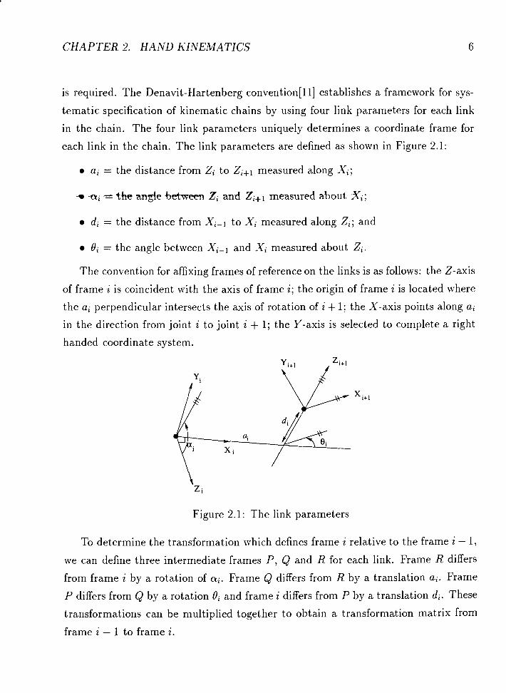
each link in the chain. The link parameters are defined as shown in Figure 2.1:
a; = the distance from 2; to Zi+1 measured along Xi;
* -a; = t he angle between Z; and Zi+1 measured about Xi;
d; = the distance from Xi-1 to Xi measured along 2;; and
6; = the angle between Xi-1 and X; measured about Zi.
The convention for affixing frames of reference on the links is as follows: the Z-axis
of frame i is coincident with the axis of frame i; the origin of frame i is located where
the ai perpendicular intersects the axis of rotation of i + 1; the X-axis points along ai
in the direction from joint i to joint i + 1; the Y-axis is selected to complete a right
handed coordinate system.
Figure 2.1: The link parameters
To determine the transformation which defines frame i relative to the frame i - 1,
we can define three intermediate frames P, Q and R for each link. Frame R differs
from frame i by a rotation of a;. Frame Q differs from R by a translation a;. Frame
P differs from Q by a rotation 6; and frame i differs from P by a translation d;. These
transformations can be multiplied together to obtain a transformation matrix from
frame i - 1 to frame i.

CHAPTER 2. HAND KINEMATICS
2.1.2 Forward Kinematics
Forward kinematics involves finding the position and orientation of the end-effector
relative to some coordinate system given a set of joint angles for each joint. Using
the link parameters defined in the previous section, we can define a transformation
matrix f-'T that transforms a vector in frame i - 1 to frame i.
Once the link parameters are found for each link and the corresponding link frames
have been defined, finding the forward kinematic equation is straightforward. The
individual link transformations can be multiplied together to find the single transfor-
mation O,T that relates frame n to frame 0.
i-1 ; T =
The matrix :T represents the last link's position and orientation in the Cartesian
space.
For a planar 3 link kinematic chain, the value of the link parameters a; and cl; are
0, so the transformation matrix :T reduces to
where sl..., and cl.,., are shorthand notations for sin(& +. . . + O n ) and cos(O1 +- . $8,)
respectively, and 11, 12, and l3 are the lengths of the links. From (2.3), the planar
coordinates x , y and orientation 6 are clearly
- - cos 4; - sin 19; 0 a;-1
sin 4; cos cos 8; cos a;-1 - sin a;-1 - sin ~ ; - ~ d ;
- sin 4; sin cos 8; sin a;-1 cos a;-1 cos ~ ; - ~ d ;
0 0 0 1 - -
(2.1)

C H A P T E R 2. HAND KINEMATICS
2.1.3 Inverse Kinematics
The inverse kinematics problem is essentially the reverse of the forward kinematics
problem. Inverse kinematics involves finding the joint angles of each link of a kine-
matic chain given the end-effector location and orientation. This problem has been
extensively studied in both computer graphics and robotics. Since inverse kinematics
is the main focus of this thesis, a detailed description and analysis of the related work
will be presented in the next chapter. The following sections will give a brief overview
of the application areas of inverse kinematics in both computer graphics and robotics.
Inverse Kinematics in Computer Graphics
The area within computer graphics that makes extensive use of inverse kinematics
is computer animation, in particular, the animation of articulated figures. An ar-
ticulated figure is usually represented by a collection of kinematic chains connected
together. Each joint in this articulated structure may have one, two, or three de-
grees of freedom. The degrees of freedom of an articulated structure increases with
its complexity. As an example, a detailed approximation of the human skeleton may
have in excess of two hundred DOF. Although well understood traditional animation
techniques [25] help animators produce expressive motions in their animation, they
require extensive manipulation of the figure to achieve the desired effects. It is obvi-
ously a very difficult task to create animation by manipulating joint angles to set up
key frames that place end-effectors of certain kinematic chains in desired locations.
Multiple iteration of trial and error is generally required to produce the correct result.
This approach is certainly very time consuming and error prone.
It is apparent that inverse kinematics offers an attractive solution to the above

CHAPTER 2. H A N D KIiVEMATICS 9
problem. Instead of letting the animator specify the joint angles that place the end-
effector at a desired location, the computer automatically calculates these joint angles
from the link configuration and the end-effector location specified by the animator.
This technique was used by Girard and Maciejewski [2S] to build the PODA system
which synthesizes the kinematic model of legged locomotion. Zhao and Badler 1471
proposed an algorithm that can incorporate various constraints and solve for simulta-
neous goals. Mielman 1451 has presented two very distinct inverse kinematic algorithms
suitable for real time manipulation and showed their effectiveness in a powerful in-
teractive editor LifeForms. By formulating inverse kinematics into an optimization
problem, Bawa [4] has presented an algorithm which uses an iterative nonlinear con- ,
strained optimization algorithm for solving the inverse kinematics problem.
Inverse Kinematics in Robotics
The inverse kinematics problem was first extensively studied in the field of robotics.
Since computer based robots are usually driven in joint space but the objects to
be manipulated are expressed in the world coordinate system, the inverse kinematic
solution is essential in controlling the position and orientation of the end-effector of
the robot arm to reach its objects.
There are two classes of solution methods for the inverse kinematics problem:
closed form and numerical. In robotics, a closed form solution is usually desired
for the kinematic chain of a robot arm rather than a numerical solution. Numerical
solutions are generally much slower than the corresponding closed form solution. Also,
numerical solutions are not generally guaranteed to converge to the correct solution
if they converge a t all. It is therefore hard to predict the quality of the solution and
the amount of time required to obtain the solution. For these reasons, researchers in
robotics usually restrict their attention to closed form solutions.
The closed form solution of a kinematic chain can be obtained by one or both of
the two solution methods: algebraic and geometric. Various algebraic methods include
the inverse transform method[34], screw algebra[20], dual matrices[lO], and the dual
quaternion method [46]. Lee and Ziegler[26] have presented a geometric method
CHAPTER 2. H A N D IXVEI1lATICS 10
to solve the inverse kinematics problem for the PUMA robot. A more thorough
discussion of closed form solution methods can be found in [14].
Hand Model
Two components of hand model are presented in this thesis: an internal skeletal
model is developed for the inverse kinematic calculations and a polygonal model for
representing the outer skin of the hand. In much of the literatures involving animation
of the hand [36, 44, 71, a simple three link pin joint model is often used internally to
represent the fingers and for the computation of joint angles. It is, however, found to
be insufficient in our application. The reasons will be made clear in Chapter 4. We
have developed an internal skeletal model which generalizes the simple pin joint model
by considering the effects of the finger joints. After the joint angles are calculated, the
hand must be displayed on the screen. This is accomplished using a surface polygonal
model of the hand. The following sections discuss each of the two components in
detail.
2.2.1 Human Hand Anatomy
The hand is one of the most complex mechanisms in the human body as it has more
than 25 degrees of freedoms. There have been numerous studies of the anatomical
structure of the hand [2, 42, 431, anatomical representation of which is given in Figure
2.2.
The hand consists of five fingers and a palm. Each of the index finger, middle
finger, ring finger and little finger has three joints. The joint closest to the palm
is called the metacarpopha langea l joint, or the MCP joint for short. This joint has
two degrees of freedom; an adduction-abduction range of approximately 30 degrees
and a flexion and extension range of about 120 degrees. The remaining two joint
are the p r o x i m a l in terpha langea l (PIP) joint and d i s ta l in terphalangeal (DIP) joint
respectively. They each have one degree of rotational freedom. The PIP joint has a
range of 100 degrees while the DIP joint has a range of 60 degrees.

CHAPTER 2. HAND I<IiVEMATICS
Figure 2.2: Anatomy of the human hand

C H A P T E R 2. H A N D KINEMATICS
The thumb is much more dexterous and therefore much more con~plex than the
other four fingers. The thumb's proximal joint is known as the carpometacarpa l
(CMC) joint. It has two degrees of freedom; an adduction-abduction range of about
120 degrees and flexion and extension range of about 45 degrees. The next joint
is the metacarpopha langea l (MCP) joint which also has two degrees of freedom; an
adduction-abduction range of 30 degrees and a flexion-extension range of 50 degrees.
The last joint is the i n t e rpha langea l (IP) joint which has only one degree of freedom
and has a range of approximately 85 degrees.
Biomechanical Models of the Hand
From a biomechanical standpoint, the human hand can be considered as a linkage
system of intercalated bony segments. The joints between each phalanx are spanned
by ligaments, tendons and muscles. With the contraction of muscles, these joints
can be moved in a characteristic manner constrained by the interposing soft tissues
and the bony articulation [2]. In the hand, most of the tendons span the joint and
continue their course over one or more joints, thus forming a bi-articular or poly-
articular system.
The functional anatomy of the spatial relationships between these tendons and
muscles and their associated joints have been extensively studied by Landsmeer 121,
231. Landsmeer also proposed a series of models to represent the various manners in
which tendons bridge the associated joints. However, these studies show either a lack
of quantitative description or that the information is restricted in only two dimensions.
An et al. [2] established a workable model in a three dimensional manner based on
the direct and careful measurements of 10 normal specimens. Such a model can
easily be utilized in the study of hand motion or force analysis of hand under various
functional activities. Various other studies on the tendon excursion and moment arm
of the finger can be found in [22, 24, 31. Since information about forces acting on
the finger, the tendon excursion, and the moment arm of the finger cannot easily be
obtained using non-intrusive techniques, we have to construct a kinematic model of
the hand using only the information obtainable by our equipments.

CHAPTER 2. HAND I<IArEMATICS
2.2.2 Internal Skeletal Model
In this section we develop an internal skeletal model of the hand based on anatomical
information. The hand can be considered as an articulated structure composed of rigid
segments connected by joints. Even though the palm is not completely planar, for the
sake of simplicity, it can be approximated using a plane whose normal points out from
the back of the hand. Since the joints of ihe fingers are clearly not simple pin joints,
there must be a small but significant distance separating two consecutive links at each
joint. We will call this distance the length of the joint. It is further hypothesized that
the lengths of the joints change as the joints rotate. This hypothesis will be verified
in Chapter 4. Therefore, we use functions F!(@, r!) to represent the length of the ith
joint of the j t h finger. The fingers are numbered from left to right on a right hand.
The 6j is the joint angle vector of the j th finger and ri is the joint radius of the ith
joint on the j t h finger. Clearly, if the functions @ are uniformly 0, this model would
reduce to the simple pin joint model.
MCP
1p t DIP
PIP
MCP
y Palm CMC
Figure 2.3: Internal Skeletal Model
Figure 2.3 shows a representation of a skeletal model of the hand. The black dots
on the figure represent the joints. It is evident from the figure that each finger of the

CHAPTER 2. HAND IiINEMATICS
hand is represented a series of joint and rigid links. The functions P! will be derived
in Chapter 4.
2.2.3 Polygonal Hand Model
A polygonal model of the hand is used to represent the surface of the hand. This model
consists of a list of vertices and a list of polygons, the latter forming the surface of
the hand. Each polygon is defined by four vertices in the vertex list.
Figure 2.4: Attachment of vertices onto the bone segments
Figure 2.5: Finger bending
The polygonal data of the hand is obtained by digitizing an actual human hand.
The surface polygons corresponding to each finger segment are initially unknown.
This information is required in order to bend or rotate a specified finger. To obtain
the needed information, a program was developed by Sidi Yu to allow the user to
interactively select vertices and attach them to finger segments. All vertices of the
polygonal hand model were manually attached to finger segments. Offsets from the
distal end of each finger segment to the attached vertices are stored. Figure 2.4 shows

CHAPTER 2. HAND KINEMATICS
the attachment of vertices onto the bones to create the polygonal hand model.
Finger bending is modeled by bending the finger segments and recalculating the
positions of the vertices corresponding to each finger segment. The position of the
distal end of the rotated finger segment is first calculated, then the stored vertex
offsets were added back to the new distal position of the segment to obtain the new
positions of the vertices. This process is shown in Figure 2.5. From the figure, we can
see that the positions of the vertices four to eight have to be updated when segment
B was rotates.
Chapter 3
Inverse Kinematics
Inverse Kinematics has been a practical problem in the field of robotics and computer
graphics. In the past decades, researchers in both robotics and computer science
have developed various algorithms to solve the inverse kinematics problem, but none
seemed to work well in all situations. There are obvious tradeoffs between speed and
accuracy among different classes of algorithms. In this chapter, the inverse kinematic
problem is formally stated and various common approaches are presented along with
their advantages and drawbacks.
3.1 Problem Definition
In Chapter 2, the basic notion of a kinematic chain of rigid segments has been in-
troduced. For simplicity, we will refer to a kinematic chain as a manipulator. Let x
be the position vector of the end-effector of the manipulator and 8 be the joint angle
vector of the manipulator. Then the forward kinematic problem can be formulated as
x = f(6) (3.1)
By inverting the function f , the inverse kinematic problem can be formulated as
CHAPTER 3. INVERSE IiINEMATICS
The inverse kinematic problem is difficult because the function f is usually nonlin-
ear. If the link parameters and the characteristics of the manipulator are well known
in advance, we might be able to find a closed form solution. However, for arbitrary
manipulators, we have to rely on numerical methods for solving systems of nonlinear
equations.
3.1.1 Existence of Solution
The question of whether solutions exist or not is directly related to the manipulator's
workspace. Intuitively, a workspace is a volume of space which the end-effector of the
manipulator can reach. For at least one solution to exist, the specified goal point
must lie within the workspace. There are two definitions of workspaces: dextrous
workspace and reachable workspace. Dextrous workspace is the volume of space which
the end-effector can reach with all orientations while the reachable workspace is the
volume of space which the end-effector can reach in at least one orientation. The
dextrous workspace is clearly a subset of the reachable workspace.
Consider the workspace of a two-link manipulator. If the length l1 and l2 of the
two links are equal then the reachable workspace consists of a disc of radius 211. The
dextrous workspace consists of only a single point, the origin. This example considers
a workspace in which all joints of the two-link manipulator can rotate 360 degrees.
This is rarely the case in actual configurations. When joint limits are a subset of the
full 360 degrees, the workspace is obviously correspondingly reduced.
3.1.2 Redundancy
A manipulator is kinematically redundant if it possesses more degrees of freedom than
are required to specify a goal for the end-effector. A planar arm with three revolute
joints has a large reachable workspace and any position in the interior of its workspace
can be reached with more than one orientation. Therefore, for any goal positions in
the interior of the workspace, the kinematic equations will yield multiple solutions.
The fact that a manipulator has multiple solutions can cause problems because
the system has to be able to choose one. The criteria with which to make a decision
CHAPTER 3. INVERSE KIiVEMATICS
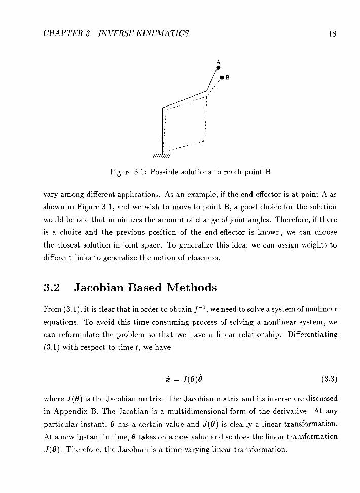
Figure 3.1: Possible solutions to reach point B
vary among different applications. As an example, if the end-effector is at point A as
shown in Figure 3.1, and we wish to move to point B, a good choice for the solution
would be one that minimizes the amount of change of joint angles. Therefore, if there
is a choice and the previous position of the end-effector is known, we can choose
the closest solution in joint space. To generalize this idea, we can assign weights to
different links to generalize the notion of closeness.
3.2 Jacobian Based Methods
From (3.1), it is clear that in order to obtain f -', we need to solve a system of nonlinear
equations. To avoid this time consuming process of solving a nonlinear system, we
can reformulate the problem so that we have a linear relationship. Differentiating
(3.1) with respect to time t , we have
where J(8) is the Jacobian matrix. The Jacobian matrix and its inverse are discussed
in Appendix B. The Jacobian is a multidimensional form of the derivative. At any
particular instant, 8 has a certain value and J(0) is clearly a linear transformation.
At a new instant in time, 8 takes on a new value and so does the linear transformation
J ( 8 ) . Therefore, the Jacobian is a time-varying linear transformation.

CHAPTER 3. INVERSE Ir'INEMATICS
3.2.1 Inverse and Pseudoinverse of Jacobian
Intuitively, J maps the incremental changes in the joint variables to incremental
changes in the end-effector position and orientation. If the matrix J is square and
nonsingular, we can compute 0 by
When this is not the case, J-' does not exist and there is no solution for e . For an
arbitrary manipulator, the Jacobian matrix J is not necessarily square and invertible.
Therefore, a generalized form of the inverse J-' is required that yields a "useful"
answer for e in the same form as (3.4):
A commonly used generalized inverse J+ is the Moore-Penrose pseudoinverse[6]. It is
shown in [5] and [6] that the Moore-Penrose pseudoinverse yields the minimum norm
solution for the under determined case and the least squares solution for the over
determined case.
3.2.2 Singularities
Most manipulators have values of 0 for which the Jacobian becomes singular. Such
locations are called singularities. When a manipulator is in a singular configuration,
it has lost one or more degrees of freedom. This means that there is some direction
along which it is impossible to move the end-effector no matter what joint rate is
selected. The two common classes of singularities are
Workspace boundary singularities are those which occur when the manip-
ulator is fully stretched out or folded back on itself such that the end-effector is
near or at the boundary of the workspace.

CHAPTER 3. INVERSE I<INEMATICS
Workspace interior singularities are those which occur away from the workspace
boundary and generally are caused by two or more joint axes lining up.
An in depth study of the classification of singularities can be found in [17]. When
the manipulator is in a singular configuration, the inverse of the Jacobian matrix J is
undefined. The pseudoinverse solution as defined in (3.5) yields unsatisfactory results
since there is an undesirable discontinuity a t the singularity. This often results in
oscillations and unacceptably high joint velocities.
The Singular Value Decomposition
The Singular Value Decomposition (SVD) is a powerful method for the analysis of
the kinematic properties of manipulators. The SVD theorem states that any matrix
can be written as the product of three (non-unique) matrices. Decomposing J, we
have
J = I J D V ~ (3.6)
It is also common to write the SVD of the Jacobian matrix J as vector products. For
an arbitrary Jacobian, it would be
i=l
where m and n are number of rows and columns of
(3.7)
J, and o; are diagonal elements
of D, also known as singular values. The pseudoinverse solution is easily obtained
from the singular value decomposition by taking the reciprocal of all nonzero singular
values. In particular, the pseudoinverse of J is given by
where r is the rank of J. The SVD has been used to detect and correct the numerical
instabilities that arise when the manipulator is near its singularities[45, 30, 29, 131.

CHAPTER 3. INVERSE IGNEMATICS
If one or more of the singular values a; are zero, then the original matrix is itself
singular. The ratio of the largest singular value t o the smallest one is called the
condition number of the matrix. If the condition number is too large, then the matrix
is ill-conditioned. This ill-conditioning is the cause of large joint velocities generated
by the pseudoinverse near a singular configuration [29].
3.2.3 Homogeneous Solution
For a redundant manipulator, a goal can usually be satisfied in a number of ways.
It is often desirable to select a solution that is optimal according to some additional
criteria. Liegeois [27] has shown that the components of the gradient of such a criterion
can be blended with the pseudoinverse solution.
e = J f i + ( I , - J f J ) V H ( B ) (3.9)
where H ( 0 ) is a potential function to be minimized, I , is the nth order identity matrix.
The first term in (3.9) essentially selects the joint velocity vector which produces the
desired change in the end-effector position, while the component ( I , - J + J ) in the
second term selects components of the gradient vector V H ( 8 ) that lie in the set of
homogeneous solutions to equation (3.4). This has the effect of varying joint velocities
in such a way that H ( 8 ) is minimized without changing the end-effector position.
Using this strategy, secondary goals can be created to avoid collisions with obstacles
as well as maintain manipulator dexterity by avoiding kinematic singularities.
3.2.4 The Jacobian Transpose Method
Although Jacobian and pseudoinverse control methods offer generality and provide
numerous ways to exploit redundancy, they suffer from several problems. First, these
methods tend to be numerically unstable near singular configurations. Also, a matrix
inversion is required at each iteration in order to obtain the joint velocity. This tends
to slow down this class of algorithms and may cause problems if the Jacobian matrix

CHL4 P T E R 3. IN V E R S E IiIiVEMATICS
is ill-conditioned. To address these problems, Welman [45] has proposed a Jacobian
transpose method which is based on a simplified dynamic model.
This method applies the principle of virtual work 1331 to obtain a linear relationship
between the external force F applied to the tip of the manipulator and the generalized
force r.
The difference between the desired position of the end-effector and the current position
of the end-effector is then used as the force F pulling on the end-effector toward
the desired trajectory. Since r is equivalent to the vector of joint acceleration e, a
simplifying assumption is made to regard r as the joint displacement dl instead of e. Therefore, the simple relationship
is obtained. Once dl is obtained, a single integration step yields a new vector B which
moves the end-effector towards the desired trajectory. The procedure repeats until
the end-effector reaches the desired position, or some other stopping criterion is met.
The Jacobian transpose method has many very attractive properties. First, there is
no matrix inversion required. This not only speeds up the computation, it also avoids
dealing with singular matrices. Also, since the computation is very simple at each
step, the algorithm is able to provide real-time feedback to the user. Since the method
is based on a simplified dynamic model, the solutions obtained in successive iterations
are predictable. The end-effector of the manipulator is continuously pulled toward the
desired trajectory by a force generated with the end-effector position error. Therefore,
successive iterations would yield configurations that are close to each other and at the
same time toward the goal. This characteristic makes the algorithm especially suitable
for interactive applications in which intermediate solutions are often needed to refresh
the screen.

CHAPTER 3. INVERSE I i INEMATICS
A major drawback of this algorithm is that it does not address joint limits directly.
Instead, joint limits are enforced by clamping to the upper and lower bounds. This
might cause the algorithm to be trapped at an intermediate configuration and stopped
only when the maximum number of iterations is reached. In addition, the algorithm
is not completely immune to singular configurations since the Jacobian matrix itself
is inherently ill-conditioned. Oscillations and high joint velocities can result near a
singular configuration.
3.3 Optimization Based Methods
A different approach to solving the inverse kinematic problem is to reformulate it
into an optimization problem and then apply the standard algorithms of nonlinear
optimization to solve it. Since a positional goal of the end-effector can be viewed as
a simple positional constraint, we can set up an objective function and minimize it
subject to a set of constraints. This approach allows us to find a solution that satisfies
multiple simultaneous constraints [35, 471. The problem is generally formulated as
minimize P ( 8 )
subject t o I; 5 8; < u; i = 1. . . n
where P ( 8 ) is the objective function to minimize, I; and u; are the lower and upper
joint limits respectively.
The flexibility offered by the optimization formulation of the inverse kinematic
problem enables us to specify various kinds of goals. Objective functions can be set
up for each of them. A detailed discussion of different categories of goals and their
corresponding objective functions can be found in [47].
Solving the constraint optimization problem is not a trivial task. It is still a rel-
atively new research area that produces collections of numerical methods for each class
of problem. Rosen's projection method is very effective in treating linear constraints[37].
Goldfarb combined the DFP method (a variable metric method) [12] with Rosen's pro-
jection method [16]. After that, the variable metric method was significantly improved
CHAPTER 3. INVERSE IiINEMATICS
by the BFGS formula [38].
Zhao and Badler have applied nonlinear optimization techniques to their animation
system Jack. Their animation system specifies a configuration of an articulated figure
as spatial constraints. The constrained parts of the articulated figure are the end-
effectors and their counterpart in space are called goals. A goal can be as simple as a
position, an orientation, a weighted combination of position and orientation, a line, a
plane, a direction, and so on, or it could be as complicated as a region in the space.
The optimization algorithm used in Jack is able to adjust the joint angles subject
to joint limits so that the set of end-effectors concurrently attempts to achieve their
respective goals. After the end-effectors and the goals are specified by the users, the
system computes a final configuration. Since it is often impossible to satisfy all the
goals owing to the actual constraints, the system outputs the best possible solution
according to the users' assignment of importance to each goal.
Bawa [4] has proposed another iterative nonlinear constrained optimization algo-
rithm to solve the inverse kinematic problem. This algorithm combines the augmented
Lagrangian method [ls] and the projected Lagrangian method 1151 to achieve super-
linear convergence. An animation system was built by Bawa that allows real-time
manipulation of the end-effectors to demonstrate this technique. Similar to the Jack
animation system, Bawa7s system is also able to handle multiple simultaneous con-
straints. In addition, a trajectory can be associated with each end-effector over a
period of time to create a complete animation sequence. Furthermore, real-time per-
formance of this animation system is ensured by the use of efficient matrix inversion
techniques.
Although the optimization formulation of the inverse kinematic problem has many
advantages, it has some drawbacks as well. Because of the complexity of the problem
and the scale of the search space, there is no guarantee that the optimizer will find
a global minimum (or maximum). As a result, it may not return the best solution
to the problem. Also, because of the iterative nature of the solution methods, it is
hard to estimate how much time the optimizer will spend on a particular problem.
Furthermore, since the optimizer is not constrained to search in any fixed direction,
intermediate solutions may not be suitable for refreshing the screen even if the screen

CHAPTER 3. INVERSE IiINEMATICS 25
needs to be refreshed because the optimizer spends a long time to obtain a particular
solution.
Table Based Method
In the efforts toward representing hand postures using a limited number of sensors,
Amaya et al. [I] have proposed an algorithm that utilizes a lookup table to solve
the inverse kinematic problem. Since this method is the predecessor of the algorithm
proposed in this thesis, it will be discussed in detail. The notation used in Amaya's
paper is discussed in Appendix A.
There are several motivations for the development of Amaya's algorithm. First,
it is well known that optical motion tracking systems cannot effectively deal with
the possibility of the occlusion of markers [32]. If we were to use the direct approach
described in Section 1.2 which places an IRED on each joint and tip of the fingers, then
the space in which the hand can freely move around without having any IREDs going
out of the camera's view would be very small. As a result, only limited movements of
the hand can be measured. This motivates the use of inverse kinematics to estimate
the hand posture, since only one IRED is need at the tip of each finger to obtain the
joint angles of that finger. This effectively enlarges the space in which the hand can
freely move around without causing occlusion of IREDs.
A second motivation for the development of Amaya's algorithm was the need for
speed in real-time computation. The Optotrak system continuously sends positional
data of IREDs to the data collection system. If a significant amount of time is required
for the computation of finger joint angles, then the data collection system would not
be able to keep up with Optotrak system. This means that the data collection system
would have to discard some incoming data and try to keep up with the Optotrak
system by computing and displaying the most recent hand posture. Because the
inverse kinematic equations are very complex and difficult to solve given a small time
frame, Amaya et al. have suggested using a lookup table to speed it up.
Given particular constraints of finger motion, there are few sets of joint angles
that correspond to fingertip positions with respect to the palm. Therefore, if we

C H A P T E R 3. INVERSE KINEMATICS
have a table of fingertip position versus orientation, we can lookup the orientation of
the fingertip given its position. Using this information from the table, only simple
calculations are required to obtain the joint angles. Thus, the basic approach behind
Amaya's algorithm is to build a lookup table of finger tip orientations using additional
IRED information before the start of the actual data collection. Then, this lookup
table is searched during data collection to obtain the current finger tip orientation
which we can use to compute the joint angles with minimum effort. This approach
suggests that the algorithm should proceed in two stages: a preprocessing stage before
data collection to build the lookup table and a run-time stage which uses the lookup
table to compute the joint angles.
The lookup table built by the preprocessing stage uses the location of the finger
tip as an index for the corresponding orientation. Amaya et al. made the assumption
that the position of the finger tip with respect to the root of the finger uniquely
defines the orientation of the fingertip. The validity of this assumption is discussed in
Section 3.4.3. The orientation is then used to determine the joint angles of the finger.
The orientation of the finger tip is obtained in the preprocessing stage by placing
additional IREDs on the finger tip as shown in Figure 3.2. However, during run-time,
only one IRED is needed at the tip to obtain its coordinates with respect to the root
of the finger. The orientation of the finger tip at run time is obtained by using this
finger tip coordinate to index into the lookup table.
3.4.1 Preprocessing Stage
The preprocessing stage consists of several steps:
1. Registration: The positional measurement of the IREDs mounted on the hand
with respect to the Optotrak workspace.
2. Table Building: The recording of position and orientation of the fingertip with
respect to the hand as the finger joints are rotated.
3. Data Filtering: The filtering and regularization of the data recorded in the
Table Building step.

C H A P T E R 3. INVERSE KINEMATICS
Figure 3.2: IRED placement in the preprocessing stage of Amaya's algorithm.
Regist rat ion
In the registration step, the lengths of the segments of the index finger and the thumb
are measured using a caliper. The hand is then placed palm down on top of its scanned
image on a fixed, rigid and flat surface as shown in Figure 3.2. Mounted on the back
of the hand are three IREDs and on the tip of the finger are mounted another three
IREDs. The positions of these IREDs in the Optotrak space (or global space) are d;,;
and di:i. Recall that d,h,; (di:;) represents the position of the ith IRED on the hand
(fingertip) in the global coordinate system. The following measurements are taken in
the global coordinate system:
0 The position of the MCP joint (1 X-Y-Z point). It is done by scanning the
subject's hand and placing an IRED on the MCP joint of the scanned image.
0 The position of the fingertip (1 X-Y-Z ~ o i n t ) . It is also done by placing an
IRED on the finger tip of the scanned hand.
0 The position of the IREDs mounted on the back of the subject's hand (3 X-Y-Z
points). The subject's hand is placed on top of the scanned hand.

CHAPTER 3. INVERSE KINEMATICS 28
The position of the IREDs mounted on the tip of the subject's finger (3 X-Y-Z
points). The subject's hand is placed on top of the scanned hand.
Using these initial measurements on the subject's right hand, the following trans-
formations and vectors are defined:
a 0: - The position of the MCP joint in global space.
0 [B;] - The orthonormal orientation of the MCP joint in global space.
0it - The position of the fingertip in global space.
[Bit] - The orthonormal orientation of the fingertip in global space.
x h - The x axis of the hand coordinate system lying along the vector from the
MCP joint to the fingertip in the plane z = 0.
y h - The y axis of the hand coordinate system pointing to the right.
0 z h - The z axis of the hand coordinate system which is pointing out of the back
of the hand.
0 xjt - The x axis of the fingertip coordinate system lying along the vector from
the MCP joint to the fingertip in the plane s = 0.
yj t - The y axis of the fingertip coordinate system pointing to the right.
0 z j t - The z axis of the fingertip coordinate system which is pointing out of the
back of the hand.
The hand and fingertip coordinate systems are shown in Figure 3.3. Since zh, yh and
zh, are unit vectors and they represent a right handed system, the transformation
matrix [B,"] is orthonormal. In particular, [B,"] satisfies

CHAPTER 3. INVERSE KINEMATICS
i '' /Finger Tip Coordinate System
Coordinate System
&-yg 2% Global Coordinate System
Figure 3.3: The hand and fingertip coordinate systems
where I is the identity matrix.
The positions of the IREDs, d& and d::,i, with respect to the hand and fingertip
coordinate frame are computed as
The vectors d;, and d;:, will be used to compute the rotation and translation
of the hand and fingertip coordinate system within the global system. Vectors with
identical superscript and subscript are assumed to be constant through all phases of
the process following their measurement.
Table Building
It is assumed by Amaya et al. that the position of the fingertip in relation to the MCP
joint in the hand coordinate system uniquely defines the orientation of the fingertip.
Thus, a subject is asked to move his finger as extensively as possible to try to fill out

CHAPTER 3. INVERSE KINEMATICS
the complete workspace of the finger. In the table building process, the hand and
finger tip coordinate systems are constructed using the three IREDs on the fingertip
and the three IREDs on the palm. This is done by writing the unit vectors pointing
along each of the three axes into the columns of the transformation matrix. The
origin of these fingertip and hand coordinate systems are translated to the finger tip
position and the MCP joint respectively. Mathematically, this can be expressed as:
The goal is to create a mapping from fingertip position to fingertip orientation
in hand space. Thus, we measure the position and orientation of the fingertip with
respect to the hand.
Recording sufficiently many of these pairs, < O;~,[B:~] >, while the finger joints
rotate creates the table which defines the mapping we need (i.e. given a position
0Lt7 we can look up a transformation to orient the fingertip in the hand coordinate
sys tem) :
Map : 0Lt + [Bit] (3.21)
However, the recorded pairs are scattered and usually sufficiently sparse that for
any particular value of 0Lt there is unlikely to be a particular tuple < OLt, [Bit] > in Map. Since we are interested in the specific [B;'] for a given OLt, we will use the

CHAPTER 3. INVERSE IXVEMATICS 3 1
notation [Bhft(p)] to represent an idealized l C h p where p is a particular value of 0;
and [Bhft(p)] is the corresponding value of [Bhft] in the map.
Data Filtering
For values of Oit where a corresponding value of [13it] is not available from Map,
Amaya et al. suggest using a 3D Gaussian filter over all of the entries in Map.
where [Bit()] is the fingertip orientation lookup table, dif , is the position of the - f t fingertip, dh represent the neighbors of d& in [B;~()], and w(a) is a Gaussian with
standard deviation a (in millimeters). It is suggested by Amaya et al. that a value
of 8mm is sufficient for a. The calculation required to compute the 3D Gaussian
convolution is very expensive under the real time experimental system. Instead, this
computation is performed at regularly spaced grid points as a batch process. The grid
used has 28 x 24 x 20 points with a point separation of 5mm. This grid of values,
indexed by Oit, contains filtered values of [Bit] and is called Map'. At run time,
simple linear interpolation is used to obtain the intermediate values. The lookup
table is shown in Figure 3.4. The black dots on the figure represent the table entries.
3.4.2 Run Time Stage
After Map' is created, for any value of 0;' we can quickly perform a simple linear
interpolation of the nearest eight values in Map' for the corresponding value of [Bit].
During run time, there are still three IREDs placed on the back of the hand in
order to determine the orientation of the hand but only one IRED is placed on the tip

CHAPTER 3. INVERSE KINEMATICS
Figure 3.4: The lookup table in Amaya7s Algorithm
Figure 3.5: IRED placement at run time

CHAPTER 3. INVERSE I\IINEMATICS 33
of each finger as shown in Figure 3.5. These IREDs are not required to be placed in
exactly the same position as in the preprocessing stage. The positions of the IREDs
on the back of the hand with respect to the hand and fingertip coordinate system are
determined using equations (3.13) and (3.14). Since there is only one IRED at the
fingertip, it is necessary to transform the indices of the fingertip orientation map from
the position of the fingertip to the position of the IRED. This is accomplished by
where d::,, is the vector from the fingertip position OLt to the IRED mounted on the
finger in the fingertip space. This is illustrated in Figure 3.6. At experiment time, we
know:
0 d{> - The measured position of the finger IRED in the hand coordinate system.
This position changes as the finger joints are rotated.
0 d::,, - The measured position of the fingertip IRED in the fingertip coordinate
system. This position is constant and is established at the registration step.
0 [~hf~(0i~)] - The orientation of the fingertip in the hand coordinate system given
the position of the fingertip. This orientation is constant and is established in
the calibration and filtering step.
Thus the unknown is O i t . In order to use Mapf, we need to build a second index
into it so that we can use the measured value of d&. We can build this index using
Equation (3.25). For each entry in Mapf, given the value of d;ivl, we can compute
the value of dL:, that will be measured at experiment time corresponding to the
appropriate tuple < 0(', [B/'] >. Linear interpolation is used to compute the value
of 0(' and [B/'] for specific values of d&.
After the orientation of the fingertip is obtained, we can use it to find the position
of the DIP joint. This is done by subtracting the length of the segment from the DIP
joint to the fingertip from the current position of the fingertip in the opposite direction
of the current orientation of the fingertip. Using the location of the DIP joint, we

C H A P T E R 3. INVERSE KINEMATICS
Figure 3.6: The known and unknown vectors when estimating the orientation and position of the fingertip
can solve for the position of the PIP joint by considering the two proximal segments
of the fingers as a two link manipulator with the end-effector fixed at the DIP joint.
Craig [9] discusses various analytical methods for solving two link manipulators.
3.4.3 Discussion
This table lookup based inverse kinematic method has several merits. Since the finger-
tip position to orientation map is built prior to the start of the real time experiment,
the computation required to obtain the joint angles is kept to a minimum. Its superior
computational speed makes it quite suitable for real time applications. Also, calibra-
tion is done for each individual subject and the fingers' workspace is also traced out
by the subject. Doing so will not only avoid interior and boundary singularities, but
also ensure that the computed hand posture closely resembles that of the actual hand
posture of the subject. Furthermore, all the constraints and joint limits are directly
built into the lookup table since it is constructed using only hand postures attain-
able by the subject. Therefore, no constraint violation needs to be checked before
displaying the computed hand posture.
All methods have drawbacks in one way or another and the table based method
is no exception. This particular construction of the lookup table relies heavily on
the assumption that the position of the fingertip in relation to the MCP joint in the
hand coordinate system uniquely defines the orientation of the fingertip. The result
produced by this algorithm may not be valid if this assumption fails. In addition, the

C H A P T E R 3. INVERSE IiINEMATICS
algorithm first calibrates for the length of each finger segment and makes the assump-
tion that the finger segments are rigid so their lengths will be constant throughout.
Although the uniqueness assumption is valid if one assumes the finger joints are
simple pin joints, the measured length of a finger segment may be perturbed by
skin movement during an actual experiment. Further, since the joints of the finger
are clearly not simple pin joints, the previous assumption is invalid even without
the effect of skin movements. The result is that inconsistent measurement of finger
segment lengths will occur during an experiment. The accuracy and even existence of
the computed joint angles rely heavily on the accuracy of the finger segment length
measurements. This is because the internal skeletal model is assumed to be a simple
pin joint model. If the measured segment lengths are longer than the actual lengths,
the set of computed joint angles is surely going to be inaccurate. Even worse, if
the measured segment lengths are shorter than the actual lengths, the goal is simply
beyond the reach of the finger and no solution can be computed.
This drawback of Amaya's algorithm often causes the data collection system to
discard data sent by the Optotrak system simply because the finger segment length
measurements do not match the initial calibration measurements. Therefore, we need
to develop an algorithm which has the desirable properties of Amaya's algorithm and
at the same time addresses its drawback. The algorithm we developed to do just this
is described in Chapter 4.
3.5 Summary
In this chapter, we have reviewed some of the most commonly used techniques for solv-
ing the inverse kinematic problem. Each method consists of distinct advantages and
disadvantages. Problems inherent in one method may not exist in another. Tradeoffs
between generality and speed are apparent. For instance, optimization based methods
tend to be more general in the sense that they can handle problems with an arbitrary
number of links having a set of possible constraints for each link. However, algorithms
for nonlinear optimization tend to be slow due to its complexity. By comparison, the
Jacobian based methods are faster, but they are not very good at handling constraints.

CHAPTER 3. IN VERSE ICINEMATICS
The fastest method presented in this chapter is the table based method. Because of
the number of assumption it made about the configuration of the manipulator and
its workspace, this method can only be applied to a small well known set of simple
manipulators. Since the human finger can be considered to be a simple three link
manipulator with a small number of constraints, the table based method seems to be
appropriate.

Chapter 4
A Table Based Real-time
Algorithm
The table based method presented in Chapter 3 provides a quick way of obtaining
inverse kinematic solutions for simple manipulators. Because of the demand for speed
in real time applications and because the human finger can often be considered as a
simple three link manipulator, the table based method is ideal for our application.
In this chapter, a table based method which addresses the problems discussed in
Chapter 3 and which is specifically designed to model the human finger is presented.
This method is relatively simple to implement and provides good performance for the
intended application.
4.1 Motivation
The method presented by Amaya et al. [I] as discussed in Chapter 3 makes the
assumption that the human finger is a simple three link manipulator with one degree
of rotational freedom at each joint. Because the joint of the finger is much more
complex than a simple pin joint and because the IREDs cannot be placed at the
center of each joint, this assumption becomes invalid.
For any simple three link pin joint manipulator, it is necessary that the dis-
tance from the end-effector to the base is a maximum when the manipulator is fully
CHAPTER 4. A TABLE BASED REAL-TIME ALGORITHM
stretched, or 8 = 0. We can express the distance between the finger tip and the root
of the finger as:
where ptip is the location of the fingertip, p,,, is the location of the MCP joint, and
d z , is the distance between them.
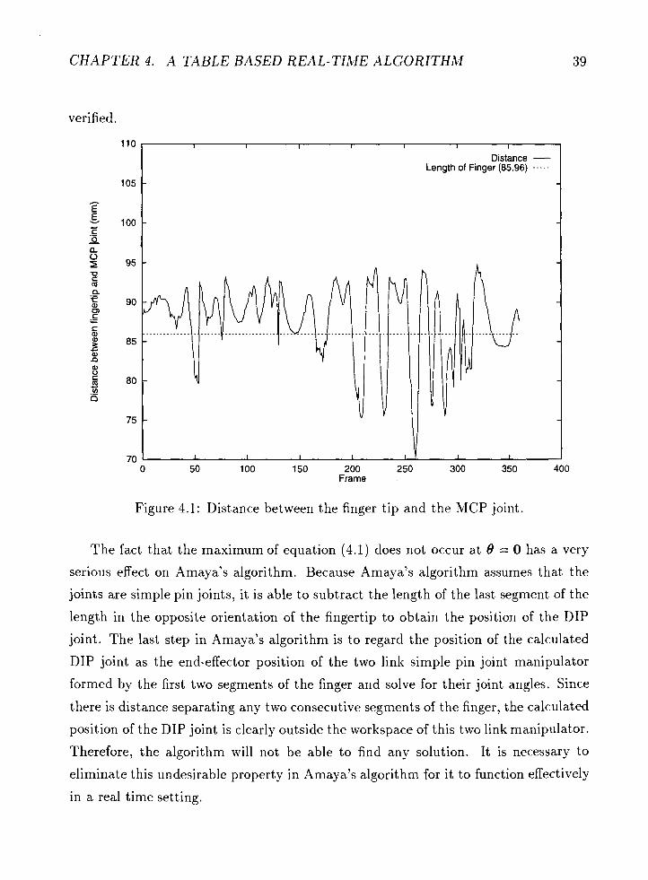
An experiment was conducted to verify whether the maximum of equation (4.1)
occurs when a real finger is fully stretched, i.e. when 8 = 0 . The length of each
segment of the index finger is measured: the length of the segment from the MCP
joint to the PIP joint was 45.8mm, the length of the segment from the PIP joint to the
DIP joint was 20.lmm, and the length of the segment from the DIP joint to the tip was
20.0mm. These measurements were first taken using the Optotrak system and then
confirmed manually using a ruler. An IRED was placed on both the fingertip and the
MCP joint of the index finger. The distance between the fingertip and the NICP joint
was measured as the finger rotates. The result is shown in Figure 4.1. The dotted
line represents the sum of three segment lengths measured when the index finger is
fully extended. The solid line is the distance between the fingertip and the MCP joint
measured by the Optotrak as the index finger rotates. By examining the recorded
joint angles of the index finger, it is clear that the maximum of equation (4.1) did not
occur when the index finger was fully extended. Furthermore, a significant number
of measured distances between the fingertip and the MCP joint are greater than the
sum of the segment lengths. However, the difference between the measured maximum
distance and the length of the finger is surprisingly large (about 10mm). Because
of this unexpected result, the experiment was repeated five times. The results from
these experiments were similar. This shows that the finger joints are clearly not pin
joints. Thus, there must be a small distance separating any two consecutive segments.
Recall that we have called this separating distance the length of the corresponding
joint in Chapter 2. Moreover, we also know that the length of the joints vary as a
function of the corresponding joint angles, for otherwise the maximum of equation
(4.1) would have occurred at 8 = 0. Therefore, our hypothesis in Chapter 2 has been
CHAPTER 4. A TABLE BASED REAL-TIME ALGORITHM
verified.
I I I
Distance - Length of Finger (85.96) - - - - -
200 Frame
Figure 4.1: Distance between the finger tip and the MCP joint.
The fact that the maximum of equation (4.1) does not occur at 0 = 0 has a very
serious effect on Amaya's algorithm. Because Amaya's algorithm assumes that the
joints are simple pin joints, it is able to subtract the length of the last segment of the
length in the opposite orientation of the fingertip to obtain the position of the DIP
joint. The last step in Amaya's algorithm is to regard the position of the calculated
DIP joint as the end-effector position of the two link simple pin joint manipulator
formed by the first two segments of the finger and solve for their joint angles. Since
there is distance separating any two consecutive segments of the finger, the calculated
position of the DIP joint is clearly outside the workspace of this two link manipulator.
Therefore, the algorithm will not be able to find any solution. It is necessary to
eliminate this undesirable property in Amaya's algorithm for it to function effectively
in a real time setting.

CHAPTER 4. A TABLE BASED REAL-TIME ALGORITHM
4.2 IRED Placements
Before the hand posture can be estimated, IREDs will have to be strategically placed
on the hand to allow the Optotrak system to track their positions. This section
discusses the IRED placements required for calibration as well as for real-time exper-
iments. For the remainder of this chapter, the i th IRED position in the Optotrak
coordinate system is denoted as d; .
4.2.1 IRED positions
In order to track the position and orientation of the hand, IREDs have to be placed
on the dorsal surface of the hand. There are two different IRED placements: one
for calibration and the other for run time. The calibration step is necessary in order
to obtain the auxiliary parameters of the finger; these parameters are the length of
each segment of the finger, the radius r; of the i th joint, and an additional parameter
p which will be discussed in the next section. After these parameters are collected,
unneeded IREDs are removed so that only a minimal number of IREDs are left.
This minimal configuration of remaining IREDs ensures that the occlusion problem
of the Optotrak system is minimized and the movement of the fingers and the palm is
not severely restricted by IRED visibility. Since the hand is not flat, any movement
of the palm or bending of the fingers may block one or more IREDs from the view
of the camera. Figure 4.2 shows some common situations in which one IRED can go
out of the view of the Optotrak camera.
Calibration
During calibration, the thickness of the finger at each joint is measured. the joint
radius r; of the i th joint is simply one half of the thickness measured at the i th joint.
The thickness is easily measured with a caliper.
The length of each of the finger segments is measured using the IRED placements
shown in Figure 4.3. The hand should be placed palm down on a flat table and the
fingers be fully extended.

CHAPTER 4. A TABLE BASED REAL-TIME ALGORITHM
Optotrak Camera
. .
. .
. . . . . . . Area visible to the . . . . . . . . . . .
. . . . . . _. . . . . Optotrak camera . . . . . . . . . . . . :..- ,_.. . .
. . : .....A/ . ,..:;, . .
Figure 4.2: Various cases that an IRED could become invisible to the Optotrak camera
The length of each individual segment can be calculated by computing the distance
between IREDs placed at the ends of each segment. IREDs 3 , 4 , and 5 define the
plane of the palm. The final calibration step measures the ratio between the angles
of the DIP and the PIP joints of the index finger. We will call this parameter p.
Rijpkema and Girard [36] suggested that there is a linear relationship between O,;,
and Odip:
We can use this relationship to simplify the table building process as discussed in
Section 4.3 .2 . The parameter p is computed as the slope of the least squared line that
passes through the data points (O,;,,, O d i p , ) in the O p i p O d i p plane.

CHAPTER 4. A TABLE BASED REAL-TIME ALGORITHbl
Figure 4.3: IRED placement for measuring segment lengths.
where n is the number of samples taken. As we will see in the description of the actual
algorithm, this parameter is used to build the lookup table for the index finger.
Run Time
At run time, all but those needed would be removed from the hand. IREDs 7 t o 9
will be taken off so that we are only measuring the position of the tips of the index
finger and thumb, the position of the MCP joint of the thumb and the orientation of
the hand. The remaining IREDs are shown in Figure 4.4.
4.3 Hand Posture Estimation
With the position of IREDs 1 to 6 given by the Optotrak system, we can now estimate
the hand posture. In this section, a simple hand model will be given first, following

CHAPTER 4. A TABLE BASED REAL-TIME ALGORITHM
Figure 4.4: IRED placement for real-time experiment
which the algorithm that estimates the hand posture from a limited number of IREDs
will be presented.
4.3.1 The Proposed Hand Model
The hand model presented in Chapter 2 is generic in the sense that the inner workings
of the finger joints are represented by unknown "black box" functions F!(B', p ) . Since
accurate biomechanical simulation is not the intent of our application, only a simple
model of the joint is used. This section describes this simple model and discusses
some of its assumptions.
Applying the theory of opposition space [19,31], we can represent the grasping be-
havior of the hand using only two fingers: the index finger and the thumb. Therefore,
our simple hand model consists only of those two fingers and the palm. It is assumed
that the index finger has four degrees of freedom: the MCP joint has two degrees of
freedom while the DIP and PIP joints each have one degree of freedom. The thumb
is assumed to have five degrees of freedom: the CMC and the MCP joints each have
two degrees of freedom while IP has one degree of freedom. For a normal hand, it

CHAPTER 4. A TABLE BASED REAL-TIME ALGORITHM
is easy to see that the fingertip, the PIP joint, the DIP joint, and the MCP joint of
the index finger lie approximately on the same plane. Furthermore, any movement
of the hand (without any external force applied to it) cannot change this property.
Therefore, we can reasonably assume that all segments of the index finger lie on a
single plane. Similarly, the tip of the thumb, the IP joint, and the MCP joint of the
thumb lie approximately on the same plane, so we can again assume that the thumb
segments between these joints lie on the same plane. As a result, a simple 2D model
can be used to represent the fingers. The palm of the hand is simply represented by
a plane and its orientation represents the orientation of the hand.
The hand coordinate system is such that the x axis is pointing in the direction of
the index finger when it is fully extended. The y axis is pointing out of the back of
the hand. The origin of the hand coordinate system is located at the MCP joint of
the index finger. The z axis points to the right to complete a right handed coordinate
system. Let x,, y,, and z, be unit vectors in the global coordinate system pointing
in the direction of the x, y and z axes of the hand coordinate system respectively. Let
P be the plane containing the palm and its normal is just the vector y, pointing out
from the back of the hand.
Figure 4.5: A circular joint
To develop a model for the finger, it is necessary to examine the finger joints
more closely. The joints that control the rotation of the segments of the finger have a
complicated structure of bones, muscles, and tendons. Since the IREDs are placed on
the dorsal surface of the finger, our measurement of joint rotation is also affected by
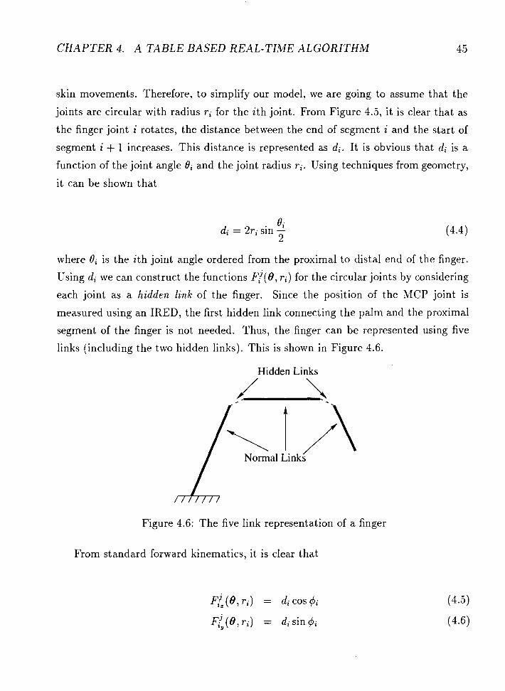
CHAPTER 4. A TABLE BASED REAL-TIME ALGORITHM 4 5
skin movements. Therefore, to simplify our model, we are going to assume that the
joints are circular with radius r; for the i th joint. From Figure 4.5, it is clear that as
the finger joint i rotates, the distance between the end of segment i and the start of
segment i + 1 increases. This distance is represented as d;. It is obvious that d; is a
function of the joint angle 8; and the joint radius r;. Using techniques from geometry,
it can be shown that
0 i d; = 2ri sin - 2
where 8; is the i th joint angle ordered from the proximal to distal end of the finger.
Using di we can construct the functions F ' ( 0 , r; ) for the circular joints by considering
each joint as a hidden link of the finger. Since the position of the MCP joint is
measured using an IRED, the first hidden link connecting the palm and the proximal
segment of the finger is not needed. Thus, the finger can be represented using five
links (including the two hidden links). This is shown in Figure 4.6.
Hidden Links
Figure 4.6: The five link representation of a finger
From standard forward kinematics, it is clear that

CHAPTER 4. A TABLE BASED REAL-TIME ALGORITHM 46
To derive the formula for 4; , we can simply consider the finger as an ordinary five
link manipulator with the special property that the sum of the two joint angles at
each end of each hidden link sum to the value of the corresponding original joint angle
of the joint in which the hidden link represents. From Figure 4.7, it is obvious that
the angles labeled a and b are the same and a + b = 6;. Therefore, we can express 4; as :
Figure 4.7: Calculation of 4;
Extending the forward kinematic equations presented in Chapter 2, the location
of the tip of the index finger can be expressed explicitly as a function of the modified
joint angles 4;.
a: = 11 cos 41 + dl cos 42 + l2 cos d3 + d2 cos $q + l3 cos $5
Y = 11 sin 41 + dl sin 42 + 12 sin 43 + d2 sin 44 + l3 sin $5 (4.8)
where (I, y) is the coordinate of the fingertip in the plane in which the index finger
lies in. A similar equation can be set up for the thumb. Since both the index finger
and the thumb have more DOF at the base, this simple model can only calculate a

CHAPTER 4. A TABLE BASED REAL-TIME ALGORITHM 4 7
subset of their joint angles. The following is the convention used for naming the joint
angles:
0 Index Finger:
- O F d e x is the rotation about the y axis at the MCP joint.
- O F d e x is the rotation about the z axis at the MCP joint.
- O F d e x is the rotation about the z axis at the PIP joint.
- O F d e x is the rotation about the 5 axis at the DIP joint.
0 Thumb:
- OAhumb is the rotation about the y axis at the CMC joint.
- BEhumb is the rotation about the z axis at the CMC joint.
- Oihumb is the rotation about the y axis at the MCP joint.
- O ~ h u m b is the rotation about the z axis at the MCP joint.
- 1 9 ~ ~ " " ~ is the rotation about the z axis at the IP joint.
The superscripts index and thumb are used to distinguish the joint angles of the
index finger and the thumb. The values of O p d e x , O F d e x l B;humbl and O ~ h u m b can be
determined using the lookup table a t run time. The values of the remaining joint
angles are calculated separately.
Since Oindex represents the rotation of the MCP joint of the index finger about
the y axis, we can calculate it by taking the dot product of the vector s, with the
projection of the vector going from the position of the MCP joint to the index fingertip
onto the plane P representing the palm. Let t = -*. be the unit vector from the II 1- 311
MCP joint to the fingertip. This calculation is illustrated in Figure 4.8.

CHAPTER 4. A TABLE BASED REAL-TIME ALGORITHM
Figure 4.8: Calculation of 82dex
Notice that the angle a between t and the plane P is the sum of the joint angle O F d e x
and an angle ,B, where P is the angle between t and the vector (d8 - d3) . The angle
a can be easily obtained by taking the dot product of x, and t . We can obtain ,O by
rotating the vector (d8 - dg) to align with the vector [l, 0,0], and moving it to the
origin. Then, using the value of O p d e x and O F d e x from the lookup table, we can obtain
the position vector t' = [ t i , t&, 0] of the fingertip evaluating the forward equation once.
The cosine of the angle ,B is then the dot product of the vector [l, 0,0], and [ t i , tk, 01.
Therefore, 8FdeX can be easily obtain by
olndex = a - p
The calculation of O F d e x is illustrated in Figure 4.9.
Since we are measuring the position of the MCP joint of the thumb, OAhumb and d -d O:humb can be calculated very easily. Let m = -&--& be the unit vector that goes
I I 6 - 411
from the CMC joint of the thumb to the MCP joint. The joint angle Okhumb can be
calculated by projecting the vector m onto the plane P. The dot product of this
vector and 2, gives the cosine of this angle. This is illustrated in Figure 4.10. Then
Okhumb can be expressed as

CHAPTER 4. A TABLE BASED REAL-TIME ALGORITHM
Figure 4.9: Calculation of r3;"dex
MCP . : . .
Figure 4.10: Calculation of 0LhUmb
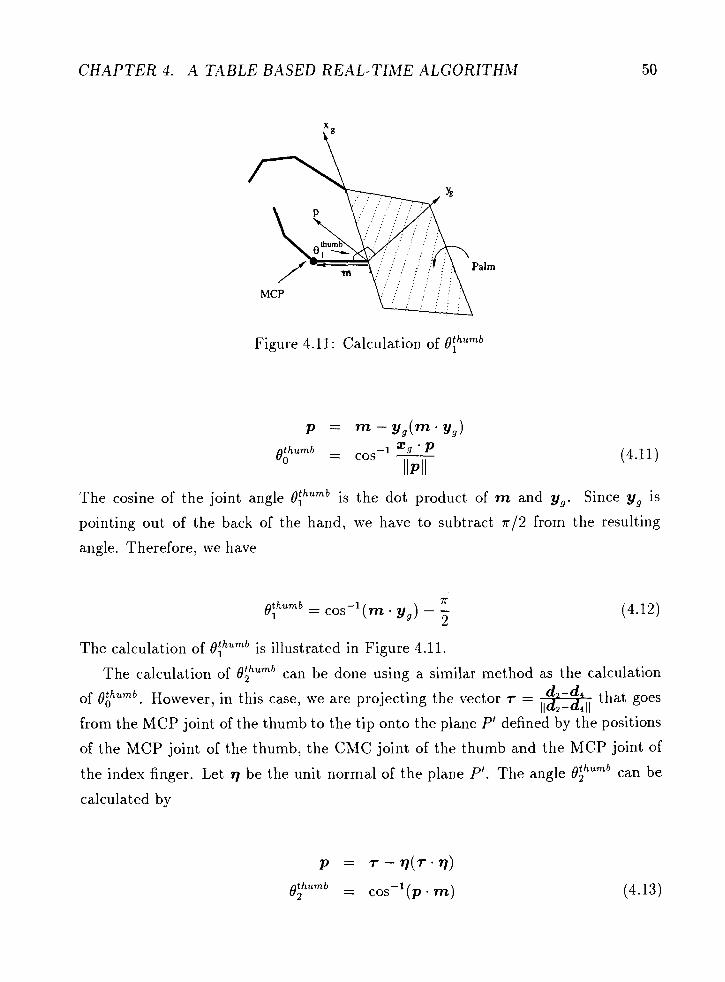
CHAPTER 4. A TABLE BASED REAL-TIME ALGORITHM
MCP
Figure 4.1 1: Calculation of 1 9 ~ ~ " ~ ~
- 0Ahumb - cos -1 xs ' P
IIPII The cosine of the joint angle B ~ h u m b is the dot product of m and y,. Since y, is
pointing out of the back of the hand, we have to subtract 7r/2 from the resulting
angle. Therefore, we have
The calculation of BEhumb is illustrated in Figure 4.11.
The calculation of B ~ h u m b can be done using a similar method as the calculation
of Okhumb. However, in this case, we are projecting the vector T = d -d .w that goes 2 - 411
from the MCP joint of the thumb to the tip onto the plane Pi defined by the positions
of the MCP joint of the thumb, the CMC joint of the thumb and the MCP joint of
the index finger. Let I) be the unit normal of the plane P'. The angle ohhumb can be
calculated by

CHAPTER 4. A TABLE BASED REAL-TIME ALGORITHM
Figure 4.12: Calculation of 19%~""~
With the above expressions for the joint angles of the index finger and thumb, the
simple hand model is complete. The following section will demonstrate how this model
is used to estimate the hand posture using live data from the Optotrak system.
4.3.2 The Algorithm
Like Amaya's algorithm, this algorithm can also be divided into two stages: the
preprocessing stage and the run time stage. The preprocessing step builds the lookup
table while the run time step simply searches the lookup table for the solution using
an appropriate index.
The algorithm for building the lookup table is very simple. The algorithm Buildln-
dexTable is given in Appendix C.1. As shown in Figure 4.4, we are measuring the
location of the tip and the MCP joint of the index finger, so the entire kinematic chain
of the index finger consists of five links (including the two hidden links). Similarly,
there are three links between the tip and the MCP joint of the thumb. Before we can
build a table, we have to select a way to index it. Instead of using the coordinate
of the tip of the finger as the index as in Amaya's algorithm, we have chosen to use

CHAPTER 4. A TABLE BASED REAL-TIME ALGORITHM
Figure 4.13: The lookup table build using the algorithm described in the thesis
the distance lltll between the fingertip and the MCP joint as the index. Since this
distance is a floating point number, we convert it to an integer before we use it as the
index. The index has a range of Omm to 200mm. By default, the interval between
successive indices is lmm. If denser indices are required, it can be specified using the
parameter p as discussed in Appendix C.1. For any values of p less than 1, we have to
scale lltll up by corresponding factor l l p and use the integer part as the index. The
next step is to evaluate the forward kinematic equation for various values of the joint
angles and insert these joint angle values into the lookup table using the calculated
index for each entry. It is possible that more than one set of joint angles have the
same index. In that case, an array is used to store all of them and the corresponding
entry in the lookup table points to the array. The index finger and the thumb have
different parameters, so a different lookup table is built for each. The lookup table
build using this algorithm is shown in Figure 4.13. The numbers c; in this figure
represent the number of sets of joint angles a; having the same index Ilt,ll.
Since the value of O1 does not affect the value of the index, 0 can simply be
assigned as its value throughout. Since there are only three links between the tip and
the MCP joint of the thumb, we can easily transform the algorithm BuildIndexTable

CHAPTER 4. A TABLE BASED REAL-TIME ALGORITHM 53
in Appendix C.1 into an algorithm BuildThumbTable by removing the inner FOR loop
and change the five link forward kinematic equations to the three link equations.
As an alternative to BuildIndexTable, we can use the parameter p to decrease the
size of the lookup table. Since we know the ratio between the joint angles O2 and
03, we can remove the inner FOR loop from the BuildIndexTable and set O3 to pOz.
Because only one FOR loop is required, the size of the lookup table only increases
linearly as the precision of the joint angles increases. This significantly increases the
table building process as well.
At run time, the lookup table is searched to obtain a subset of the joint angles
of the finger. The remaining joint angles are computed on the fly. The run-time
algorithm is given in Appendix C.2. The norm of the vector t is computed to obtain
the index. Because of the nature of our data, there might be more than one set of
joint angles that have the same index. An array is used to store all of them. Since this
array is relatively small in size, a linear search algorithm can be employed to find the
set of joint angles according to some criteria. In our application, it is assumed that the
relative angular change from one frame to the next is small. Therefore, the searching
criterion is to minimize the change from the set of joint angles in the previous frame.
It is possible that the table entry corresponding to the computed index is empty. In
this case, the algorithm would then try to find the closest table entry which contains
a t least one set of joint angles.
The algorithm GetIndexJointAngles finds the joint angles of the index finger. Sim-
ple modifications to GetIndexJointAngles can be made to change it into GetThumb-
JointAngles which finds the joint angles of the thumb. The necessary modifications
are:
Change the first line from lltll := /Idl - d311 to := /Id2 - dsll
Replace O F d e x and Opdex with Oihumb and Oihumb
Delete all references of O F d e x
Change the three link forward equations that calculates the value of t: and t',
to the two link equations.

CHAPTER 4. A TABLE BASED REAL-TIME ALGORITHhl
0 Replace the calculation of O;;"dex by the equations (4.1 I) , (4.12) and (4.13).
0 Change the last line to RETURN {Ohhumb, O~humb, Oihumb, Oihumb, O ~ h u m b ) .
4.4 Implementation
A complete data collection system which integrates data collection, estimation and
display of hand postures has been implemented to allow the experimenters to collect
accurate 3D hand posture data.
4.4.1 The Data Collection System
There are several modules in the data collection system: getlength, getRntio, getDntn,
and ikHand. The first two modules are used for the calibration step while the last
one is used during the run-time step. With the IREDs placed on the subject's hand
as shown in Figure 4.3, the first module getLength sets the Optotrak camera to a
frequency of 60Hz and measures this calibration hand posture for 0.5 seconds for a
total of 30 frames. The lengths of each finger segments are computed a t each frame
and the average lengths are then written to a file length.dat. When the second module
getRatio is invoked, the subject is asked to freely rotate and bend his fingers. The
getRatio module collects this data for six seconds and computes the parameter p used
to build the lookup table using equation (4.3). The value of p is written to ratio.dat.
Before the start of the run-time stage, the thickness of the finger at each joint would
have to be measured using a caliper. The values of the thickness data are stored in
thickness.dat. Now, we have completed the calibration stage.
At the run-time stage, IREDs 7, 8, and 9 can be taken off the hand. After that, the
module ikHand is invoked. It again sets the Optotrak camera to 60Hz and continuously
collects the positional data of the IREDs. The program computes the hand posture
at each frame from these positional data and displays the resulting hand posture onto
the SGI monitor. The collected data is not written to a file since it is very slow to
display and access the file system at the same time. If the data needs to be stored,
the module getData can be used to collect and store the data into a file hand.dat. The

CHAPTER 4. A TABLE BASED REAL-TIME ALGORITHM
stored data can later be viewed using a modified version of the module &Hand which
gets the input from a file instead of getting it from the Optotrak system. A sample
display is shown in Figure 4.14.
Implementation Details
The main data struciure used in this system is the lookup table. It is implemented
as a dynamic array. Each element of the table is another dynamic array. This is used
to store different sets of joint angles having the same index (Iltll). At the run-time
stage, the value of the index is computed from the live 3D data and this value is
used directly to index into the lookup table to obtain the array of sets of joint angles
having this index value. Since size of this array is very small (usually around three
and four), a linear search algorithm is used to determine which set of joint angles has
the minimum deviation from the joint angles of the previous frame.
All modules are implemented in C++ on a Silicon Graphics Indigo2. The Open
Inventor Library is used to do the vector calculations and rendering of the hand.
4.5 Discussion
The table based inverse kinematic algorithm presented in the previous section uses
the lookup table approach introduced by Amaya et al. to solve the inverse kinematic
problem. It addresses some of the weaknesses of Amaya's algorithm by making addi-
tional assumptions about the finger and joint configurations. In particular, it utilizes
the notion of hidden joints to simulate the behavior of the finger joint and account for
the error introduced by skin movement. In addition, this algorithm is stable in the
sense that it will always return a feasible solution. It is easy to see from the algorithm
that it always returns the optimal solution in which the end-effector position error
is minimized. Furthermore, the computational speed is not jeopardized by the accu-
racy and stability of the algorithm. The algorithm is very fast because no coordinate
transformation needs to be explicitly performed. This also means that numerical er-
rors associated with the transformation of coordinate system are eliminated as well.
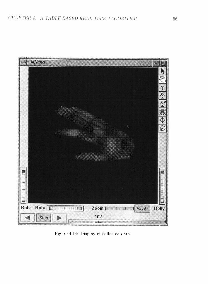
Figure 4.14: Display of collected dat,a

CHAPTER 4. A TABLE BASED REAL-TIME ALGORITHM
However, unlike Amaya's algorithm in which the lookup table has to be regularized to
obtain uniform table entries, there is no clear way to do regularization on the lookup
table built by this algorithm. Since there can be more than one set of joint angles
stored in a single entry, simple interpolation of the table entries cannot be done to
obtain a regularized table. Furthermore, even if interpolation is applied to two entries
in the table to obtain an entry between them, there can be no guarantee that the
interpolated joint angles will produce the desired index.
Unlike the Jacobian based algorithms presented in Chapter 3, this table based
algorithm does not explicitly address the singularity problem. Instead, this problem
is avoided by finding the closest feasible solution in the workspace. Also, joint limits
are usually hard to enforce using Jacobian based algorithms. It is usually done by
clamping the joint angles to the maximum or the minimum limit. Handling joint
limits this ways may produce unnatural looking joint angles. In our algorithm, joint
limits can be explicitly specified in the table building process, so any solutions that
lie outside the joint limits will not be returned.
One of the major drawbacks of this algorithm is that it cannot be readily extended
to handle other manipulators. The algorithm is specifically designed to simulate the
human finger. Furthermore, it assumes that the relative angular movement between
the previous frame and the current frame is small. However, even in our application,
it is possible for the Optotrak camera to miss some frames as the IREDs became
hidden from its view. As a result, the next valid frame may be drastically different
from the previous valid frame. In this case, the solution returned by the algorithm
will be extremely unpredictable. Fortunately, there are many entries in the lookup
table that contain only a single set of joint angles. The joint angles of the previous
frame are only used to select among different choices. Since there are no choices if
one of those entries is selected by the algorithm, this problem would vanish.

Chapter 5
Experiment and Results
This Chapter describes an experiment which applies the algorithm presented in Chap-
ter 4 in a real-time setting and discusses the results obtained from the experiment.
The main purpose of the experiment is to evaluate the accuracy of the algorithm and
demonstrate that it can be effectively used in a real-time setting.
5.1 The Real-time Experiment
In order to evaluate the accuracy of this table based method, a practical experiment
was performed. After setting up the equipment, the preprocessing stage begins by
placing the subject's hand palm down on a flat table. The IREDs were placed as
shown in Figure 4.3. The equipment setup is shown in Figure 5.1. This calibration
posture of the subject's hand was sampled at 6OHz for 0.5 second. The lengths of
the finger segments were computed at each frame. Then, the average lengths of the
segments from the 30 sampled frames were used as the measured lengths of the finger
segments to build the lookup table. The subject was then asked to freely move and
rotate the index finger and the thumb. This data was sampled at 6OHz for six seconds.
The PIP and DIP joint angles of the index finger were computed at each frame and
used to obtained the parameter p using equation (4.3). The lookup table was built
using an accuracy of p = 0.1 which means value of the joint angles stored in each
entry of the table is accurate to l/lOth of a degree. The hand motion data was again

CHAPTER 5. EXPERIMENT A N D RESULTS
Figure 5.1: Equipment setup
collected a t 6OHz for six seconds for a total of 360 frames.
During the run-time stage, only six IREDs were needed as shown in Figure 4.4.
To determine the accuracy of the methods, the IRED placement was not changed
from the preprocessing stage. Since there is an IRED on every joint of both the index
finger and the thumb, the actual joint angles and the position of the fingertips can be
easily measured. However, the only IRED information given to the inverse kinematic
algorithm was the position of the six IREDs required to compute the joint angles in
run-time. The computed joint angles were compared with the actual joint angles to
determine the accuracy of our method. In addition, the actual position of the fingertip
is compared with the computed fingertip position obtained by evaluating the forward
kinematic calculations using the computed joint angles.

CHAPTER 5. EXPERIiWWT AND RESULTS
5.2
One of
IREDs
Difficulties Encountered
the major difficulties encountered during the experiment was the occlusion of
from the Optotrak camera. It is obvious that the hand is not a flat surface,
so as the hand rotates and the fingers bend, one or more of the IREDs placed on the
hand are inevitably going to be blocked from the view of the camera. As a result,
much of t h e data returned by the Optotrak system was rendered useless. This also
severely restricts the workspace of the hand. Furthermore, the quality of solution
from our algorithm can be severely affected since the table based algorithm requires
the joint angles of the previous frame as initial approximation for the joint angles in
the current frame. If IREDs in several consecutive frames between one valid frame
of data and the next were blocked from the camera, the algorithm would have to
use the last valid frame (not the previous frame) to approximate the joint angles of
the current valid frame. This is usually not a good approximation and the algorithm
will probably return poor results. One possible solution to this problem would be to
surround the subject with Optotrak cameras, so all the IREDs will be in the view of
at least one camera at all times. This solution, however, cannot be implemented at
the time of this writing because of the high cost of the equipment.
Another problem encountered during the experiment was the speed of rendering
the hand in real-time. As discussed in Chapter 2, the graphic hand is composed
of many polygons. A significant amount of time is spent in drawing them. In ad-
dition, deformation calculations are performed in real-time to simulate the bending
and stretching of the finger. With the additional overhead of polling data from the
Optotrak system and computing joint angles using our algorithm, the graphic hand
was not able to be rendered quickly enough to give the illusion of smooth hand move-
ment. However, after hand tuning the matrix computations used in the deformation
and speeding up the calculation ~erformed for the inverse kinematic algorithm, the
graphic hand can now be rendered at approximately 12 frames per second on a Silicon
Graphics Indigo2 Extreme. As suggested by Welman [45], 10 frames per second is the
minimum for interactive applications to maintain the illusion of continuous interactive
control.

CHAPTER 5. EXPERIMENT AND RESULTS
Actual DIP joint angle - Computed DIP joint anlge - - - - -
100 150 200 250 Frame
Figure 5.2: Comparison of B!Jdex

CHAPTER 5. EXPERIMENT AND RESULTS
Actual PIP joint angle - Computed PIP joint anlge - - - - -
0 50 100 200 250 300 350 400 Frame
Figure 5.3: Comparison of OFdex

CHAPTER 5. EXPERIMENT AND RESULTS
Actual MCP joint angle - Computed MCP joint anlge - - - - -
. . . . . . . .
0 50 100 150 200 250 300 350 400 Frame
Figure 5.4: Comparison of O;"dex

C H A P T E R 5. EXPERIMENT A N D RESULTS
Measured x - Computed x - - - - -
0 50 100 150 200 250 300 350 400 Frame
Figure 5.5: Comparison of the x coordinate of the tip of the index finger
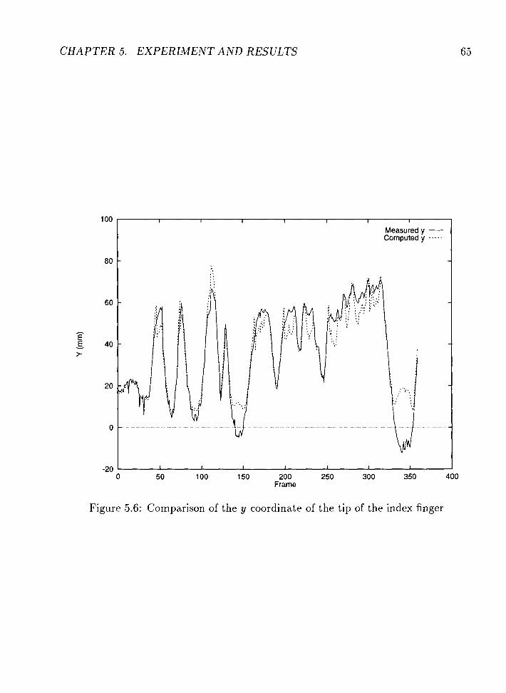
CHAPTER 5. EXPERIMENT AND RESULTS
Measured y - Computed y ---- .
-20 0 50 100 1 50 200 250 300 350 400
Frame
Figure 5.6: Comparison of the y coordinate of the tip of the index finger

CHAPTER 5. EXPERIMENT AND RESULTS
120 I I I I I 1 1
Error -
200 Frame
Figure 5.7: The error between measured tip location and computed tip location of the index finger
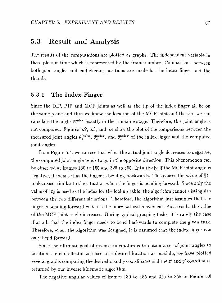
CHAPTER 5. EXPERIMENT A N D RESULTS
5.3 Result and Analysis
The results of the computations are plotted as graphs. The independent variable in
these plots is time which is represented by the frame number. Comparisons between
both joint angles and end-effector positions are made for the index finger and the
thumb.
5.3.1 The Index Finger
Since the DIP, P IP and MCP joints as well as the tip of the index finger all lie on
the same plane and that we know the location of the MCP joint and the tip, we can
calculate the angle OFdex exactly in the run-time stage. Therefore, this joint angle is
not compared. Figures 5.2, 5.3, and 5.4 show the plot of the comparisons between the
measured joint angles OFdex, OFdex, and OFdex of the index finger and the computed
joint angles.
From Figure 5.4, we can see that when the actual joint angle decreases to negative,
the computed joint angle tends to go in the opposite direction. This phenomenon can
be observed at frames 130 to 155 and 320 to 355. Intuitively, if the MCP joint angle is
negative, it means that the finger is bending backwards. This causes the value of lltll
to decrease, similar to the situation when the finger is bending forward. Since only the
value of lltll is used as the index for the lookup table, the algorithm cannot distinguish
between the two different situations. Therefore, the algorithm just assumes that the
finger is bending forward which is the more natural movement. As a result, the value
of the MCP joint angle increases. During typical grasping tasks, it is rarely the case
if at all, that the index finger needs to bend backwards to complete the given task.
Therefore, when the algorithm was designed, it is assumed that the index finger can
only bend forward.
Since the ultimate goal of inverse kinematics is to obtain a set of joint angles to
position the end-effector as close to a desired location as ~ossible, we have plotted
several graphs comparing the desired x and y coordinates and the x' and y' coordinates
returned by our inverse kinematic algorithm.
The negative angular values of frames 130 t o 155 and 320 to 355 in Figure 5.6

CHAPTER 5. EXPERIMENT AND RESULTS
confirmed that the index finger is indeed bending slightly backwards. Figure 5.7
shows the error between the desired coordinate (xi, yi) and the computed coordinate
(x:, Y:). The error e; of the i th frame is computed using the formula
The average error of Figure 5.7 is 6.01mm.
5.3.2 The Thumb
The data collected for the thumb is compared in a similar way. Since we measure the
position of the CMC and the MCP joint of the thumb at run-time, we can calculate
the joint angles OhhUmb and OihUmb exactly. Also, we know that the MCP and the IP
joints as well as the tip of the thumb all lie on the same plane, we can calculate the
joint angle OihUmb exactly using equation (4.13). Therefore, the only two joint angles
obtained using the lookup table are OihUmb and OjhUmb. The comparison results are
shown in Figures 5.8 and 5.9.

CHAPTER 5. EXPERIMENT AND RESULTS
Actual IP joint angle - Computed IP joint anlge - - - - - I
150 200 250 300 350 400 Frame
Figure 5.8: Comparison of O:h"mb

CHAPTER 5. EXPERIMENT A N D RESULTS
Actual MCP joint angle - Computed MCP joint anlge - - - - -
0 50 100 150 200 250 300 350 400 Frame
Figure 5.9: Comparison of 0ihumb

C H A P T E R 5. EXPERIMENT AND RESULTS
I I I I I I I
Measured x - Computed x - - - - -
-20 1 I I 1 I I I I I 0 50 100 150 200 250 300 350 400
Frame
Figure 5.10: Comparison of the x coordinate of the tip of the thumb
Notice that the difference between the measured joint angles and computed joint
angles from frame 200 to 300 in both Figures 5.8 and 5.9 are quite large. The values of
the measured joint angles are large in that interval while the values of the computed
joint angles are relatively small. This error could be caused by any one or a com-
bination of two sources. Since the thumb is extremely dextrous, the skin movement
on the thumb is very significant. An IRED was placed on top of the MCP joint and
on the tip of the thumb to measure their distance. This distance is the value of the
index into the lookup table. If the position of the IRED measuring the position of the
MCP joint is severely affected by skin movement, the value of the index would not be
computed very accurately. This could cause serious error in our computation. Also,
since the radius of the IP joint (including the IRED thickness) is estimated using a
ruler, it might not be very accurate. This introduces additional error into our com-
putation. Placing the IREDs on rigid materials that are tightly fixed to the thumb

CHAPTER 5. EXPERIMENT A N D RESULTS
100 - I I I I I I I
Measured y - Computed y - - - - -
-
-
Frame
Figure 5.1 1: Comparison of the y coordinate of the tip of the thumb

CHAPTER 5. EXPERIMEiVT AND RESULTS
I
Error -
0 50 100 150 200 250 300 350 400 Frame
Figure 5.12: The error between measured tip location and computed tip location of the thumb

CHAPTER 5. EXPERIMENT AND RESULTS
helps reducing errors caused by skin movement. However, this will severely restrict
the movement of the thumb. Radius estimation error can be reduced by adjusting this
radius parameter before the experiment until the computed movement of the thumb
is similar to the actual movement.
Not very surprisingly, significant errors from frame 200 to 300 are observed from
the plots of the thumb tip location. The average error of Figure 5.12 is 7.lmm.
5.4 Summary
An experiment was conducted to measure the performance of the proposed table
based inverse kinematic algorithm. From the experimental results, we can see that
the algorithm works extremely well for the index finger. Error between measured tip
location and computed tip location only becomes large when the index finger bends
backwards. Fortunately, this is rarely possible without external force exerted on the
finger. The error for the thumb becomes significant when the value of the joint angle
at the IP joint become large. This error can be reduced by eliminating skin movement
effects on IRED position and careful estimates of the IP joint radius.

Chapter 6
Conclusions
We have examined the solutions to the inverse kinematic problem applied to the
determination of hand posture in real-time. As an alternative to various algebraic
and numerical methods published in robotics and computer graphics journals, a simple
but very fast lookup table based inverse kinematic algorithm has been developed for
the computation of the joint angles of the index finger and the thumb from live 3D
positional data. This algorithm has been integrated into a complete data collection
system which is able to calibrate, collect and display hand postures of test subjects
in experiments.
A similar table based inverse kinematic algorithm was proposed by Amaya et al.
[I]. However, the algorithm presented in this thesis addresses some of its weaknesses.
The major contributions of this thesis include:
developed a more accurate model of the finger using circular joints;
developed a fast table-based algorithm which can be used effectively in real-time;
integrated the polygonal representation of the outer surface of the hand into the
display routines; and
developed a data collection system which integrates data collection, hand pas-
ture estimation and display of the hand.

CHAPTER 6. CONCL USIONS
6.1 Summary
When doing this research, it is apparent that no one single inverse kinematic algo-
rithm is uniformly superior to others and is suitable for all types of applications. For
instance, computer animations systems requires their inverse kinematic algorithms
to be able to produce "useful" intermediate solutions to refresh the screen in order
to maintain the level of interactivity. On the other hand, trajectory control systems
of robots require their inverse kinematic algorithms to produce accurate joint angle
solutions to maintain the trajectory of the end-effector of the robot. So, the ability to
produce intermediate solution is of little interest to these systems. By contrast, the in-
verse kinematic algorithms used in a real-time environment such as the one described
in this thesis, is required to process incoming data (possibly containing noise) and
produce a solution as quickly as possible. The quality of solution, of course, greatly
depends on the correctness of the incoming data as well as any measured calibration
parameters.
In Chapter 4, we have presented an algorithm which estimates a human hand
posture from a limited number of IREDs. The key to this method is lookup tables
built during a calibration step which measure the characteristics of different subjects'
hands. With this information, the run-time system determines the joint angles of both
the index finger and the thumb. The method presented provides the computational
speed required for our real-time application and reasonable approximation of the hand
postures of the subject. The solution returned by this algorithm is a compromise
between accurate end-effector position and "natural" looking joint angles since it
neither requires the end-effector to be accurately place at a particular point with no
regard to the value of the joint angles nor it tries to set the joint angles in a way that
the position of the end-effector is completely ignored. Instead, the algorithm tries to
find a set of reasonably natural joint angles such that the error between the distance of
the measured end-effector position and computed end-effector position is minimized.
In Chapter 5, the method has been confirmed to produce adequate results.

CHAPTER 6. CONCL USIONS
Future Work
Since this thesis is only a part of the efforts in trying to construct a Virtual Hand
Laboratory, there is still considerable work left to be done. First, the inverse kinematic
algorithm presented in Chapter 4 is planned to be integrated into the head tracking
system developed by Valerie Summers. This will provide a stereo view of the virtual
hand for the subject while the experiment is in progress. Also, the calibration of the
hand and the head tracking devices can be done together as one step. This will not
only save time, but will also provide additional viewing information such as location
of the viewer and so on for the display subroutine.
Since a neural network generalizes the notion of a lookup table, we would like to
investigate ways to define a neural network to solve the inverse kinematics problem.
Compared to a lookup table, the neural network has the added advantage that it
can "learn" from past results. Since a neural network is essentially a lookup table,
the processing speed would be comparable to the table based method described in
Chapter 4. Further research is needed to define the structure of the neural network
and its training method.
In order for the virtual hand to be truly useful, the occlusion problem would have
to be solved. One way to solve this problem would be to place more than one Optotrak
camera around the subject. If an IRED is occluded from the view of one camera, the
other cameras will still be able to sense its position. Because of the high cost of the
needed equipment, it is very unlikely that this method can be implemented in the
near future.
In addition, a hierarchical spline representation of the hand can be constructed to
allow for different resolutions of display of the hand. Using this property, experiments
can be done to investigate the appropriate level of realism of the graphic hand needed
to carry out a typical kinesiology experiment.
Furthermore, we plan to investigate ways to construct lookup tables having a
uniform distribution of entries. Doing so, in theory, will speed up the time required
to search the lookup table and resolve collisions present in each entry of the table.
Appendix: A
Notations Used in Amaya's Paper
Three coordinate frames are employed in Amaya's algorithm: the Optotrak "global"
frame, the "hand" frame at the MCP joint created by three IREDs on the back of
the hand, and the "fingertip" frame on the tip of the finger created by three IREDs
on the fingertip.
The matrix [B] is the basis matrix of a coordinate system where the i th basis vector
is placed at the i th column of [B] . The vector 0 is the position vector of the origin
of a coordinate system. The superscripts and subscripts on both [B] and 0 read:
Asource- f rame destination- f rame
The source frame is the frame of reference in which the input vector is currently
expressed in which the destination frame is the frame of reference in which the output
vector going to be expressed in. The positions of the IREDs are represented by the
vector d . The notation used is:
d I R E D group coordinate- f rame,IRED number
The subscripts below other vectors represent the coordinate frame of that vector

Appendix: B
Jacobian Matrix and Its Pseudoinverse
The Jacobian is a matrix of first derivatives. To derive it, we can differentiate the
elements of equation (3.1) to get
dx, = a i m a i m a f m -do1 + -dB2 + . . . + -do, a01 (302 86,
Dividing by the differential time element dt and writing in matrix notation, we have
; = ~ ( e ) c i
and clearly J is
I . . .
2.L asl ae2 . a 2& ael ae, . . . J = .
af, L a,, a,, . . U E J den
If J is not a square matrix or does not have a full rank, J-' does not exist and there
is no solution for t!l. In order to find a useful solution for 9, the generalized inverse

CHAPTER 6. CONCLUSIONS 80
of J is usually used. A commonly used generalized inverse J+ is the Moore-Penrose
pseudoinverse[6]. The pseudoinverse J+ is defined as
+ - J T J j T ) - 1 J - (
for the under determined case and
+ - J T J ) - 1 J T J - (
for the over determined case.
Appendix: C
C. l Algorithm to build the lookup table This section presents an algorithm that builds the lookup table for the index finger.
The lookup table is built by evaluating the forward kinematics equations for $ degree
increments for each of the PIP and DIP joint angles, where p is the precision of the
joint angles. The index used for the lookup table is the distance between the tip of
the finger and the MCP joint. Since the value of O1 (the MCP joint angle) does not
affect the value of the index, it is set to 0.

CHAPTER 6. CONCLUSIONS S2
ALGORITHM: BuildIndexTa ble
Input: The segment length I ; ordered from the MCP joint to the tip. The joint radius
r; of each joint. The joint li,mits for the DIP and PIP joints. The precision, p, of the
joint angle.
Output: A joint angle lookup table having lltll as its index. Each entry in the table
consists of a counter and an array of joint angles.
BEGIN
d l := 0
FOR t z := (pipLowerLimit/p) T O (pipUpperLimit /p) BY 1 DO
FOR t3 := (dipLowerLimit/p) T O (dipUpperLimit lp) BY 1 DO
82 := t2p
03 := t3p
do := 2rl sin d2/2
dl := 2r2 sin d3/2
$0 := d*
41 := 40 + 8212
4 2 := $1 + 0212
$3 := $2 + 6312
$4 := 43 + 0312
x := ll cos $1 + do cos 4 2 + l 2 cos $3 + dl cos $4 + E3 cos 45 Y := 11 sin $1 + do sin $2 + 12 sin $3 + dl sin $4 + l3 sin qh5
index := &G P
Table[index].angleList[count] := (02, 193)
Table[index].count := Table[index].count + 1
END /* FOR */ END /* FOR */ RETURN Table
END

CHAPTER 6. CONCLUSIONS
C.2 Algorithm to search the lookup table This section presents an algorithm that searches the lookup table at run-time
to obtain a subset of the needed joint angles. The algorithm first computes the
index value (the distance between fingertip and the MCP joint). Then, it looks for
the corresponding entry in the lookup table. If this entry is empty, the algorithm
searches both forward and backwards to find the closest non-empty entry. After this
entry is found, the algorithm then determines whether there are more than one set
of joint angles stored in this entry. If not, the only set of joint angles stored in this
entry is returned. Otherwise, the algorithm finds the set of joint angles which has the
minimum change from the set of joint angles of the previous frame. This set of joint
angles is then returned. This algorithm also checks to make sure that the angle P is
less than or equal to the angle cr (a and ,B are discussed in Chapter 4).

CHAPTER 6. CONCL USIONS 84
ALGORITHM: GetIndexJointAngles
Input: The lookup table. The IREDs' positional vectors d; in the global frame as in
Figure 4.4. The indez finger joint angles { i 3 ~ d e x 1 , dFder ' ) of the previ0.u~ frame. The
precision, p, of the joint angles.
Output: The joint angles of index finger for the current frame.
BEGIN
less := FALSE
minErr := maxFloat
position := 0
index := Ilt l l /p
IF Table[index].count = 0 /* i f this entry is empty */ found := FALSE
forward := index
backward := index
WHILE (NOT found) /* find first non-empty entry in either direction
* / forward := foward + 1
backward := backward - 1
found := ((Table[ f orward] .count>O) OR (Table[backward] .count > O ) )
END /* WHILE */ IF (Table[forward].count > 0) T H E N /* get search direction */
indez := forward
ELSE
index := backward
END /* IF */

CHAPTER 6. CONCLUSIONS
END /* IF */ WHILE (NOT less) /* if angle ,B is not less than a */
FOR i := 0 TO Table[index].count - 1 BY 1 DO
{02, 03) := Table[index] .angleList [i]
t: = 11 + 12 C O S ( ~ ~ ) + C O S ( ~ ~ + 63)
t& = 12 sin(&) + l3 cos(02 + 03)
p := cos- t ;
(J- 1 index1)2 + (OFdex - err := J((a - 8) - + (02 - o2 @dex')2
IF (/3 <= a )
IF (NOT less)
minErr = er r
position = i
less = TRUE
ELSE
IF (err < minEr r ) THEN
minErr = er r
position = i
END / * IF */ END /* IF */
END /* IF */ E,ND /* FOR */ IF (NOT less)
position = 0
index := index + 1
END /* IF */ END /* WHILE */ {OFdex, Ogdex) := Table[index] .angleList [position]
P := t - y , ( t . Y,)
t i = 11 + 12 cos(O2) + 13 cos(O2 + 03)
tk = 12 sin(02) + cos(02 + 03)

CHAPTER 6. CONCL USIONS
END

Bibliography
[I] Kenji Amaya, Tom Calvert, and Christine L. MacKenzie. Posture estimation of
a human hand from a limited number of markers (unpublished). August 1995.
[2] K. N. An, E. Y. Chao, W. P. Cooney 111, and R. L. Linscheid. Normative model
of human hand for biomechanical analysis. Journal of Biomechanics, 12:775-788,
1979.
[3] K. N. An, Y. Ueba, E. Y. Chao, W. P. Cooney, and R. L. Linscheid. Tendon
excursion and moment arm of index finger muscles. Journal of Biomechanics,
16(6):419-425, 1983.
[4] Sumeet Bawa. Interactive creation of animations: An optimization approach to
real-time inverse kinematics. M.Sc. thesis, Simon Fraser University, April 1995.
[5] A. Ben-Israel and T. N. E. Greville. Generalized Inverses: Theory and Applica-
tions. Wiley, New York, 1974.
[6] T. L. Boullion and P. L. Odell. Generalized Inverse Matrices. Wiley Interscience,
New York, 1971.
[7] William L. Buford and David E. Thompson. A system for three-dimensional
interactive simulation of hand biomechanics. IEEE Transactions on Biomedical
Engineering, 34(6):444-453, 1987.
[8] E.Y. Chao, J. D. Opgrande, and F. E. Axmear. Three dimensional force analysis
of finger joints in selected isometric hand functions. Journal of Biomechanics,
9:387-396, 1976.

BIBLIOGRAPHY 88
[9] John J . Craig. Introduction to robotics: mechanics and control. Addison-Wesley,
New York, 1989.
[lo] J . Denavit. Description and Displacement Analysis of Mechanisms Based on 2x2
Dual Matrices. Ph.D. thesis, Northwestern University, 1956.
[ll] J. Denavit and R. S. Hartenberg. A kinematic notation for lower-pair mechanisms
based on matrices. ASME Journal of Applied Mechanics, 23:215-221, 1955.
[12] R. Fletcher and M. J . D. Powell. A rapidly convergent descent method of mini-
mization. Co,mputer Journal, 63163-163, 1963.
[13] G. Forsythe and C. B. Moler. Computer Solution of Linear Algebraic Syskms.
Prentice-Hall, Englewood Cliffs, N.J., 1967.
[14] K. S. Fu, R. C. Gonzales, and C. S. G. Lee. Robotics: Control, Sensing, Vision,
and Intelligence. McGraw-Hill, Inc., New York, 1987.
[15] Philip E. Gill, Walter Murray, and Margaret H. Wright. Practical Optimization.
Academic Press, New York, 1981.
[16] Donald Goldfarb. Extension of Davidson's variable metric method to maximiza-
tion under linear inequality and equality constraints. SIAM J. Appl. Math.,
17:739-764, 1969.
[17] B. Gorla and M. Renaud. Robots Manipulateurs. Cepadues-Editions, Toulouse,
1984.
[IS] M. R. Hestenes. Augmentability in optimization theory. Journal of Optimization
Theory and Applications, 32427-440, 1980.
[19] Thea Iberall, Carme Torras, and Christie MacKenzie. Parameterizing prehen-
sion: A mathematical model of opposition space. pages 2-12, Proceedings of
COGNITIVA 90.
[20] D. Kohli and A. H. Soni. Kinematic analysis of spatial mechanisms via successive
screw displacements. Journal of Energy for Industry, 2739-747, 1975.

BIBLIOGRAPH k' 89
[21] J. M. F. Landsmeer. Anatomical and f~~nct ional investigations on the articulation
of the human fingers. Acta anatomica, 25:l-69, 1955.
[22] J. M. F. Landsmeer. A report on the co-ordination of the interphalangeal
joints of the human finger and its disturbances. Acta morphologica neerlando-
scandinavica, pages 59-84, 1958.
1231 J. M. F. Landsmeer. Studies in the anatomy of articulation. Acta morphologica
neerlando-scandinavica, 3287-303, 1961.
[24] J. M. F. Landsmeer. The coordination of finger joint motions. The journal of
bone and joint surgery, 45:1654-1662, 1963.
[25] J. Lasseter. Principles of traditional animation applied to 3d computer animation.
Computer Graphics, 21(4):35-44, Proceedings of SIGGRAPHS7.
[26] C. S. G. Lee and M. Ziegler. A geometric approach in solving the inverse kinemat-
ics of puma robots. IEEE Trans. Aerospace and Electronic Systems, 20(6):695-
706, 1984.
[27] A. Liegeois. Automatic supervisory control of the configuration and behavior of
multibody mechanisms. IEEE Trans. System, Man, Cybernetics, 7(12), 1977.
[28] Girard. M. and Maciejewski. A. A. Computational modeling for computer gen-
eration of legged figures. Computer Graphics, 19(3):263-270, 1985.
[29] Anthony A. Maciejewski. Dealing with the ill-conditioned equations of motion
for articulated figures. IEEE Computer Graphics and Applications, pages 63-71,
1990.
[30] Anthony A. Maciejewski and Charles A. Klein. The singular value decomposition:
Computation and applications to robotics. The International Journal of Robotics
Research, 8(6):63-79, 1989.
[31] C. L. Mackenzie and T. Iberall. The grasping hand. Elsevier Science, Amsterdam,
1994.

BIBLIOGRAPHY 90
[32] Axel Mulder. Human movement tracking technology. Technical report, School
of Kinesiology, Simon Fraser University, B.C., July 1994.
[33] R. P. Paul. Robot Manipulators: Mathematics, Programming, and Control. MIT
Press, Cambridge, MA, 1981.
1341 R. P. Paul, B. E. Shimano, and G. Mayer. Kinematic control equations for simple
manipulators. lEEE Trans. Systems, Allan, Cybern., 11(6):449-455, 1981.
[35] Cary B. Phillips, Jianmin Zhan, and Norman I. Badler. Interactive real-time
articulated figure manipulation using multiple kinematic constraints. Computer
Graphics, pages 245-250, 1990.
[36/ Hans Rijpkema and Michael Girard. Computer animation of knowledge- based
human grasping. Computer Graphics, 25(4):339-348, 1991.
[37] J. B. Rosen. The gradient projection method for nonlinear programming. SIAM
J. Appl. Math., 8:lSl-217, 1960.
[3S] D. F. Shanno. Conditioning of quasi-newton methods for function minimization.
Math. Computation, 24:647-664, 1970.
[39] D. J . Sturman. Whole-hand Input. Ph.D. thesis, MIT, 1989.
[40] David J. Sturman and David Zeltzer. A survey of glove-based input. IEEE
Computer Graphics and Applications, 14(1):30-39, 1994.
[41] S. Augustine Su and Richard Furuta. A logical hand device in virtual envi-
ronments. Technical report, Department of Computer Science, University of
Maryland, College Park, Maryland 20742, April 1993.
[42] C. Taylor and R. Schwartz. The anatomy and mechanics of the human hand.
Artificial Limbs, (2):22-35, 1955.
[43] Chor Quan Teo. A hybrid procedural/knowledge-based approach to the anima-
tion of human hand grasping. M.Sc. thesis, Simon Fraser University, February
1994.

BIBLIOGRAPHY 9 1
[44] David E. Thompson. Biomechanics of the hand. Perspectives in computing,
11(3):12-19, 1981.
[45] Chris Welman. Inverse kinematics and geometric constraints for articulated figure
manipulation. M.Sc. thesis, Simon Fraser University, April 1993.
[46] A. T. Yang and R. Freudenstein. Application of dual number quaternian algebra
to the analysis of spatial mechanisms. Trans. ASME, J. Appli. Mech., 31:152-
157, 1964.
[47] J. Zhao and N. I. Badler. Real time inverse kinematics with joint limits and
spatial constraints. Technical Report MS-CIS-90-09, Department of Computer
and Information Science, University of Pennsylvania, 1989.
[48] T. G. Zimmerman. A hand gesture interface device. In H,uman Factors in Com-
puting Systems and Graphics Interfaces, pages 189-192, April 1957.