Yale ICF Working Paper No. 10-04

Pension Fund Performance and Costs: Small is Beautiful

Rob M.M.J. Bauer Maastricht University

K. J. Martijn Cremers

Yale University

Rik G. P. Frehen Tilburg University

Electronic copy available at: http://ssrn.com/abstract=965388

Pension Fund Performance and Costs: Small is Beautiful

Rob M.M.J. Bauer, Maastricht University

K. J. Martijn Cremers, Yale University

Rik G. P. Frehen, Tilburg University

April 29, 2010

Abstract

Using the CEM pension fund data set, we document the cost structure and performance of a large sample of US pension funds. To date, self-reporting biases and a deficiency of comprehensive return and cost data have severely hindered pension fund performance studies. The bias-free CEM dataset resolves these issues and provides detailed information on fund-specific returns, benchmarks and costs for all types of pension plans and equity mandates. We find that pension fund cost levels are substantially lower than mutual fund fees. The domestic equity investments of US pension funds tend to generate abnormal returns (after expenses and trading costs) close to zero or slightly positive, contrasting the average underperformance of mutual funds. However, small cap mandates of defined benefit funds have outperformed their benchmarks by about 3% a year. While larger scale brings costs advantages, liquidity limitations seem to allow only smaller funds, and especially small cap mandates, to outperform their benchmarks.

JEL Classifications : G23, G11, G14

Acknowledgements Our thanks to Keith Ambachtsheer, CEM Benchmarking Inc. for providing the pension fund database, and Jules van Binsbergen, Dion Bongaerts, Jeffrey Brown, Mathijs Cosemans, Joost Driessen, Piet Eichholtz, Will Goetzmann, Ralph Koijen, Bruce Lehmann, Ludovic Phalippou, Geert Rouwenhorst, Peter Schotman, Allan Timmermann (WFA discussant), Laurens Swinkels, University of Amsterdam seminar participants, Q-group meeting participants, WFA 2009 and Netspar Pension Day participants for helpful comments and suggestions. Furthermore, we gratefully acknowledge research grants provided by ICPM and Netspar, and superb research assistance by Aleksandar Andonov.

Electronic copy available at: http://ssrn.com/abstract=965388

1. Introduction

Pension funds are a critical component of many people’s overall financial position and among the

largest institutional investors in the US. However, remarkably little is known about their

performance and cost structures. By contrast, the mutual fund and hedge fund sectors have been

heavily scrutinized. The lack of pension fund performance studies can be largely attributed to an

absence of sufficient data, which is a direct result of a lack of reporting guidelines. Mutual funds

are required to report their performance and fees on a regular basis, whereas no such obligation

exists for pension funds.

The main contribution of this paper is to employ the CEM pension fund database to provide a

comprehensive overview of the performance and costs of domestic equity investments by US

pension funds. The database, which does not suffer from reporting biases, covers approximately

40% of the US pension industry in terms of assets, representing a wide variety of fund sizes and

equity mandates, and contains both defined benefit and defined contribution plans. Specifically,

our database consists of 463 defined benefit pension funds for 1990–2006, and 248 defined

contribution pension funds for 1997–2006.

We find that pension fund cost levels are substantially lower than mutual fund fees, largely as a

result of scale advantages. The risk-adjusted net performance of total equity investments of the

funds (after expenses and trading costs) tends to be positive and statistically significant, though

relatively small after also benchmark-adjusting. However, small cap and smaller size mandates

tend to generate positive alpha. For example, small cap mandates of defined benefit funds

outperform their benchmarks by about 3% a year.1 These results contrast with the average

underperformance of mutual funds.

We further aim to explain cross-sectional differences in risk-adjusted returns, finding that fund

size erodes risk-adjusted performance. Further, this effect is most pronounced for investments

that are prone to liquidity risk. This explanation is consistent with large pension funds being

unable to respond quickly to news or invest large parts of their portfolio in relatively illiquid

stocks. We also give detailed insight in the variety of benchmarks used to evaluate asset managers

and the exact cost structure of pension funds.

Pension fund return data in previous work was not only limited but also typically employed on a

managed account level, i.e. returns are provided for managers employed by pension funds (see

                                                        1 Mandates are investment styles and a subset of the total equity investments of these funds. 

e.g. Beebower & Bergstrom (1977), Coggin, Fabozzi, & Rahman (1993) and Busse, Goyal, &

Wahal (2009)). This reporting structure prohibits direct documentation of the performance of

pension funds as such, since managers are often employed by more than one pension fund and

pension funds typically hire more than one manager. As a result, one typically does not know

which manager is trading for which fund and, therefore, one cannot compute fund performance.

Arguably, the largest drawback of the data collection on manager level is the inability to measure

cross-sectional differences between pension funds. Furthermore, previously used data on pension

funds typically lacked comprehensive cost data.2 Finally, our data also includes information on

the benchmarks used by pension funds, which can be used for performance evaluation and is, to

the best of our knowledge, unique to the literature.

The lack of comprehensive return, benchmark and cost data and possible self-reporting biases

have induced a broad diversity of conclusions on pension fund performance and costs.3 For

example, in the most comprehensive study on plan level, Lakonishok, Shleifer, & Vishny (1992)

show that 769 defined benefit plans lag the S&P 500 by 260 basis points yearly. Based on their

figures, it seems justified to question the future of the pension industry. However, their result is in

sharp contrast to Busse, Goyal, & Wahal (2009), who perform the most complete study on

pension fund accounts so far. They study 6,260 portfolios managed by institutional asset

managers on behalf of defined benefit pension funds. Using a conditional multi-factor model,

they find that the average fund manager outperforms the market by 124 basis points after

expenses.

The absence of consensus on pension fund performance is in marked contrast to the abundant

evidence on mutual fund underperformance. A majority of performance studies concludes that

after expenses and trading costs, mutual funds perform on average slightly worse than a

                                                        2 Apart from a small number of surveys (e.g. McKinsey (2006) and Mercer (2006)), very little has been known about the costs of pension funds. One exception is Bikker and De Dreu (2007), who focus on administration and investment costs of Dutch pension funds, which constitute only a subset of the total costs of these funds. 3 Other studies, confirming the widely diverging findings on pension fund performance, are the following: Brinson, Hood, & Beebower (1986) study 91 defined benefit plans and conclude that the funds underperform the S&P 500 by 110 basis points per year. Ippolito & Turner (1987) also document underperformance in a sample of 1,526 plans. They conclude that the S&P 500 on average has a return advantage of 44 basis points. Elton, Gruber, & Blake (2006) study mutual funds offered by defined contribution plans and show that they are beaten by the market by 31 basis points per year. Beebower & Bergstrom (1977) examine the performance of 148 US portfolios in a CAPM framework. In their study, the average portfolio outperforms the S&P 500 by 144 basis points per year. Coggin, Fabozzi, & Rahman (1993) document positive selectivity and negative timing skills for a random sample of 71 equity managers from US pension plans.  

comparable passive proxy.4

The above mentioned complications of pension fund data and the contrasting findings of earlier

pension fund studies illustrate how difficult it is to create a consistent and comprehensive picture

of the performance of the US pension industry and give insight in the benchmarks and cost

composition of this sector. The recently available CEM dataset enables us to address the

aforementioned issues, thereby strongly improving our understanding of the performance and

costs of US pension funds. The CEM database includes annual data on pension plan level, i.e. net

returns, benchmarks and costs per fund, and within each fund per mandate (see below). The plan

level data and broad coverage of the U.S. pension universe provide the opportunity to determine

which factors explain cross-sectional differences in risk-adjusted returns.

Following Kenneth French, who first used the CEM data in his AFA presidential address on the

cost of active investing (see French (2008)), we use the data set to complete the picture on cost

levels and their driving forces. By linking our data to Compustat, we are able to test for potential

biases that could result from the voluntary reporting, and ascertain that our data do not suffer

from them. On our performance evaluation, we can differentiate between several mandate types,

i.e. large versus small capitalization stocks, actively versus passively managed portfolios, and

externally versus internally managed mandates (only relevant for defined benefit funds).

We find that pension fund cost levels for their domestic equity investments are substantially

lower than in the mutual fund industry, with a median annual cost of 27 basis points for defined

benefit funds and 51 basis points for defined contribution funds, though with considerable cross-

sectional variation. Such heterogeneity in cost levels is to a significant extent driven by

differences in fund size. For example, the average annual cost levels for the smallest and largest

30% of domestic equity investments of defined benefit funds equal 40 and 15 basis points,

respectively. Irrespective of fund size, externally managed mandates are found to be significantly

more expensive than their internally managed counterparts. Similarly, actively managed mandates

have higher costs than passively managed mandates. Further, pension plan participants benefit

from the larger size of their pension plans through lower cost levels in internally managed

                                                        4 For example, Malkiel (1995) and Gruber (1996) observe that mutual funds on average underperform the market by the amount of expenses charged to investors. Chan, Chen, & Lakonishok (2002) corroborate the underperformance of the mutual fund industry in a study on mutual fund investment styles. However, more recent mutual fund performance studies have found evidence that some subset of funds may have skill. For example, Kacperczyk, Sialm, & Zheng (2005) use fund’s industry concentration, and find that funds that focus on particular industries may outperform. Similarly, Cremers & Petajisto (2009) find that funds with high Active Share, whose holdings differ significantly from their benchmark index, tend to outperform their index. 

domestic equity portfolios. Our finding that larger funds have lower cost levels in externally

managed mandates indicates pension funds’ bargaining power with external parties.

The domestic equity investments of US defined benefit pension funds tend to generate positive

abnormal returns after expenses and trading costs, contrasting the average underperformance of

mutual funds. For example, using the standard four-factor Fama-French-Carhart benchmark

model, the annualized abnormal performance of the net domestic equity returns at the overall

fund level equals 1.32% (t-statistic of 4.93). Using (self-declared) benchmark-adjusted returns,

this outperformance equals 45 basis points per year (t-statistic of 1.82). For defined contribution

funds, we generally find similar evidence for outperformance with weaker statistical significance,

which may be due to a smaller and shorter sample.

Further, it is especially small cap mandates that have positive alpha and outperform their

benchmarks. Large cap mandates have generally smaller alphas that become insignificant after

also benchmark-adjusting the net returns. However, small cap mandates of defined benefit funds

have an annualized net alpha of 3.08% (t-statistic 3.54) after also benchmark-adjusting. These

results are further robust to the choice of methodology (random coefficients model versus the

three-stage regression analysis of Brennan, Chordia and Subrahmanyam (1998)).

The positive performance of the small cap mandates is related to our other major finding that

smaller fund or mandate size is associated with better performance, similar to Chen, Hong, Huang

and Kubik (2004). While larger scale brings costs advantages, these are apparently overshadowed

by size disadvantages in equity performance. In particular, liquidity limitations seem to allow

only smaller funds, and especially small cap mandates, to outperform their benchmarks. We show

this by appending the Pastor and Stambaugh (2003) traded liquidity factor to the four-factor

model and regressing alphas on firm characteristics, including interactions with the liquidity beta.

In particular, the size of the equity holdings has a large and negative coefficient in these alpha

regressions, whereas this negative association between the size of the investments and

performance is stronger if the liquidity beta is larger, i.e. for less liquid investments.

Finally, we also consider how other fund choices are related to performance, such as how much is

invested internally versus externally, and what percentage of investments is actively versus

passively managed. In our sample, only about 12% of defined benefit investments are internally

managed (and all of the defined contribution investments are), and only 5% of their small cap

investments. In general, we find some evidence suggesting that external management performs

slightly better, with the difference being smaller for the largest internally managed mandates.

This is consistent with investments requiring a certain size in order to be able to build sufficient

expertise and profitably keep management in-house.

In conclusion, we argue that pension funds perform close to their benchmarks in the aggregate,

and on average outperform in smaller funds and mandates and in small cap mandates. We find

some evidence for scale advantages in internally managed portfolios and in bargaining power

with external parties.

The remainder of our paper is organized as follows. Section 2 introduces our data set and

measures possible self-reporting biases. In section 3, we describe our methodology. Section 4

presents the cost levels of the various equity mandates and studies the cost differences between

funds. In section 5, we present the basic performance evaluation results. Section 6 investigates the

importance of liquidity, mandate size and fund size. Section 7 concludes.

2. The Database

The defined benefit (DB) and defined contribution (DC) pension fund data are provided by CEM

Benchmarking Incorporated (CEM), which collects detailed information on pension fund costs,

benchmarks and performance via yearly questionnaires.5 While CEM collects data from multiple

asset classes and numerous countries, in this paper we focus exclusively on domestic equity

investments by US pension funds. Table 1 illustrates the evolution of this part of the database on

US pension funds, by reporting the number of funds entering and leaving the database for every

sample year. The overview shows that the number of funds in the database is relatively stable.

Therefore, it seems unlikely that our results are driven by a single year or a few funds.

The time frame of our analysis is 1990-2006 for defined benefit and 1997-2006 for defined

contribution funds, due to data availability. A total of 463 defined benefit and 248 defined

contribution funds report to CEM over the sample period. In any given year, approximately 150

defined benefit and 75 defined contribution US pension funds are included. The number of funds

entering and leaving the database is relatively stable over time. In general, pension funds decide

to enter the benchmarking process in order to benchmark their investment returns and costs

against pension funds of similar size and background. Large-sized pension funds that can afford

                                                        5 The Toronto-based company CEM Benchmarking Incorporated specializes in providing independent, objective, and actionable information to pension funds. CEM uses its expertise to compare and benchmark pension funds in a global domain and to provide best practice information to these funds. Since 1990, CEM provides benchmarking services on pension fund investments and administration. The investment benchmarking service provides DB and DC fund sponsors insights into cost, return, and risk of the investments of the funds. Information is collected from multiple asset classes and numerous countries. 

the costs of being benchmarked are more inclined to hire CEM. Pension funds also regularly

decide to leave the database. There can be several reasons for leaving the data set. Smaller and

midsized funds could stop the service in need of costs savings. Mergers and acquisitions among

the underlying corporations may cause funds to cease to exist or stop reporting. The same holds

for pension funds of companies that merge into another firm or go bankrupt in any given year.

Self-reporting Bias

Pension funds choose CEM’s services and in connection to their relationship to CEM provide

annual reports on costs levels and performance. Their reporting to CEM is voluntary, which

makes the data potentially vulnerable to self-reporting biases. Table 1 gives a first insight into

possible biases in our database. For example, if funds would stop reporting to CEM as a result of

bad performance in a certain year, one would expect higher numbers of exiting funds in years

with bad market performance, e.g. 2001 and 2002. However, Table 1 gives no indication of

higher numbers of exiting funds in these years.

We investigate the self-reporting bias by linking the CEM data set to the Compustat SFAS 158

pension database.6 The Compustat database contains the yearly returns on pension assets (ROA)

for all US corporate pension plans that have an obligation to report to the SEC, from 1998

onwards.7 Hence, the Compustat data set does not suffer from biases related to voluntary

reporting. The matching procedure resulted in matches for, respectively, 67% and 49% of

corporate defined benefit and defined contribution pension funds in the CEM database.8

We first test for self-reporting biases by categorizing the matched Compustat ROA observations

into two groups. The first group contains ROAs of years in which funds stopped reporting, i.e. the

first year that they did not report to CEM anymore. The second group contains all remaining data.

By comparing the means of the groups, we can test whether funds decide to stop reporting as a

result of bad performance.

                                                        6 In addition to the aforementioned, primary data set (containing returns, benchmarks and costs for anonymous pension funds), CEM provided us also with a secondary database containing only fund names and their entry and exit years in the primary data set and no other variables. However, this secondary database cannot (and was and will not) be linked with the primary, anonymous data source. We only matched the secondary database to the Compustat data, respecting the anonymity of the funds in the primary set containing performance, benchmark and cost figures. 7 This is the total returns over all asset classes (contrasting the equity focus of the rest of the paper). Therefore, the maintained assumption is that funds are likely to stop reporting if their overall performance is bad, i.e. this decision does not merely depend on their equity performance. 8 Funds are matched based on their names. Since some pension funds in the CEM database have no obligation to report to the SEC (e.g. because they are too small) it is impossible to match 100% of funds. Name changes are not considered as entries or exits. 

Next, we repeat this test for the year in which funds enter into our database, i.e. we categorize the

matched Compustat data into two groups, with group 1 containing all funds in years in which

they decide to report to CEM for the first time (excluding the first year of the data set) and the

second group containing all the other data. Again, we test if there is a significant difference in the

mean ROA between the two groups. This will address the question whether firms start or go back

to working with CEM after relatively good performance.

Panels A and B of Table 2 show that we find no evidence of a self-reporting bias in the exiting or

entering years. In Panel A, we report the difference in the mean ROA between the groups as

defined above, i.e., we measure the difference in mean ROA of funds in their exiting years and all

remaining data points, and likewise for funds in their entering years. The differences in mean

ROA are all insignificant (highest t-stat equals 0.40). We employ robust standard errors to adjust

for autocorrelation or heteroskedasticity. However, as most funds have observations in both

groups and irregularly enter and exit the database (see Table 1), clustering observations by funds

does not make much of a difference.

In a second test of the self-reporting bias, we conduct a logit regression of a dummy variable

indicating presence in the CEM database. As independent variables, we use the Compustat ROA

performance for the matched sample, the log of the total equity holdings of the funds, and the log

of the total equity holdings squared. We use robust standard errors and present marginal effects.

The coefficient on the fund’s total ROA is always insignificant, while larger funds are more likely

to be included in our database, as shown by the positive loading on fund size. This is consistent

with the idea that specialized benchmarking services as provided by CEM are more relevant and

cost-effective for larger funds, but gives no evidence for other self-reporting biases related to

performance.

Fund size and mandates

The unique structure of the CEM database allows for a detailed breakdown in the evaluation of

the performance and cost of domestic equity investments by US pension funds. Specifically, we

can divide each pension fund’s “mandates” in 3 different dimensions: large versus small

capitalization stocks, actively versus passively managed investments, and internally versus

externally managed equity investments (the latter separation only occur for defined benefit funds,

as all DC funds are externally managed). These 3 dimensions thus give rise to 23 = 8 possible

different combinations for DB funds (e.g. small cap – external – active, or large cap – internal –

passive) and four different combinations for DC funds. The main caveat with regards to these

mandates is that the passively managed investments could include ‘enhanced’ index funds and

could potentially further profit from stock lending programs (however, we lack more precise

information on this).

The data provided by CEM are reported at the lowest aggregation level (i.e., cost levels and net

returns on each of the 8 (for DB) or 4 (for DC) different combinations separately). As a result, we

can measure differences between investment styles. The domestic equity returns and costs levels

at the higher aggregation level are computed for each fund separately by value-weighting the

lower level returns using the equity holdings as weights. Performance is always measured net of

costs.

In Panel A of Table 3 we report the distribution of the size of the domestic equity portfolios at the

total fund level for both DB and DC funds. The median fund has $1.2 billion in domestic equity

investments with an average of $4.2 billion, such that the sample has a clear right-skewed size

distribution. The size distribution is relatively stable over time, as shown in Figure 1A for DB

funds, presenting the plot of the average log size for five quintile size groups each year.

At the fund level, most of the equity investments are made in large cap stocks (average of 89%)

and are done externally (average of 88%). Further, an average of 69% of investments is held in

actively managed mandates, the remaining being in passively managed index funds. Panel B of

Table 3 gives the characteristics for large cap and small cap mandates, indicating that large cap

mandates use more passive management (especially DC funds) and are more likely to be

internally managed (only relevant for DB funds). Both observations may largely be driven by

large cap mandates being much bigger than small cap mandates. The sheer size of the largest

funds might make active management more complicated. Cremers and Petajisto (2009) also find,

for US equity mutual funds, that larger funds in general and large cap funds in particular tend to

have lower Active Shares (i.e., portfolios whose holdings are more similar to their benchmarks).

Higher percentages of internal management for large cap mandates and larger funds can likewise

be explained by economies of scale; the larger the fund, the lower the relative costs of internal

management.

Panel C and D of Table 3 provide the statistics for the active – passive, and the external – internal

management choice, respectively. The distribution of passive mandate size is particularly right-

skewed. Allocations to small cap stocks are about three times larger for active mandates than for

passive mandates. For example, the average allocation to small cap stocks for active mandates of

DC funds equals 29%, versus 8% for passive DC mandates. Finally, the size distributions of

external versus internal mandates for DB funds seem similar. Internally managed mandates occur

much less frequently (only about 12% of investments by DB funds) and tend to be in larger funds

and largely invested in large caps (about 97%) and about 47% in passively managed mandates.

Figure 1B, 1C and 1D plot the time variation in the average percentage of equity investments, at

the fund level, held in large cap, actively managed, and internally managed mandates,

respectively, for five quintile size groups of DB funds.9 Here, as everywhere else in the paper,

size is measured using the total domestic equity investment positions only. Figure 1B shows that

DB funds have generally increased their allocations to small cap mandates over time, especially

the smaller size groups. For example, by the end of our sample (2006), the group of 20% smallest

DB funds holds an average of about 30% in small cap stocks. The choice between active and

passive management (see Figure 1C) shows no clear time trend, with the 1990 averages being

quite similar to the 2006 averages for all size quintile groups. However, larger funds have clearly

greater allocations to passive mandates. For example, the group of 20% largest DB funds holds an

average of about only 50% in actively managed mandates, while the group of 20% smallest DB

funds holds an average of about 85%. Finally, fewer DB pension fund investments have been

internally managed over time. Smaller and medium-sized funds seem to have largely abandoned

internal management, while the percentage of internally managed mandates has dropped

significantly for the largest funds. For example, for the group of 20% of largest DB funds,

internal management fell from 55% in 1990 to about 30% in 2006 (see also Table 3).

We provide cross-sectional graphs for DB funds, using data for 2006 only, in Figure 2. Figure 2A

plots the percentage allocations to small cap mandates of all DB funds against fund size, showing

that large funds tend to have greater large cap allocations. Figures 2B and 2C plot the percentage

allocations to active and internal mandates, respectively, against fund size. Figure 2B shows that

larger pension funds tend to be less active, though until $20 billion under management there

seems to be little association between fund size and allocations to actively managed mandates.

Figure 2C shows that many DB funds are completely externally managed. For those that have

internally managed mandates, these are typically combined with external management. Only four

DB funds are (almost) completely internally managed in 2006. Finally, there seems to be little

association between fund size and the allocations to internally managed mandates for the subset

of DB funds where these occur, while DB funds that are exclusively externally managed tend to

                                                        9 Analogous figures for DC funds were not included to save space, but are generally similar. In particular, DC funds have gradually increased their small cap and active allocations over our time period. 

be smaller.10

3. Methodology

This section explains the ‘random coefficients’ panel data technique used to evaluate pension

fund performance, and also describes the three-stage regression analysis, employed to test for

cross-sectional differences. Due to the annual frequency of our data, standard time-series

regression methods to calculate risk-adjusted performance cannot be employed.

The random coefficients model differs from standard pooled panel regression by allowing the

alphas and betas to vary over the cross-section, instead of assuming common parameters for all

funds. Our assumption of a common distribution for alphas and betas is less restrictive than

common parameters across funds. While being quite similar to Timmermann, Blake, Tonks, &

Wermers (2009), our methodology differs from theirs by allowing idiosyncratic risk to vary

cross-sectionally.

Specifically, the random coefficient model assumes that fund-specific alphas and betas (e.g. of

the Fama-French factors) are independently drawn from hierarchical distributions with common

parameters. The hierarchical parameters can be estimated with high precision as we benefit from

the large cross-section of our sample. Economically, the higher order parameters can be

interpreted as the pension fund industry (or some group/category of funds) alphas and betas.

We define net excess returns of fund i in year t,, )( eitR as the domestic equity return net of costs

minus the 3-month US T-Bill rate, and characterize our model as

,ittiieit FFR ηβα ++=

where we assume that iα and iβ are drawn independently from distributions with constant

means and variances, tFF the year t Fama-French factor returns and itη a normally distributed

error term with zero mean,

),(~ 2ασαα Ni ),(~ 2

βββ ΩNi ),0(~ 2ηση Nit .

We assume that βΩ is a diagonal matrix and β is a vector with factor loadings

),,,( MOMHMLSMBM ββββ . We also regress net benchmark adjusted returns )( BMitR , the difference

                                                        10 Analogous figures for DC funds are again similar but omitted to save space.  

of the net fund return and the fund’s self-declared benchmark return, on the same set of factors.

For a more detailed description of our random coefficients model, see Swamy (1970).

The Brennan, Chordia and Subrahmanyam (1998, henceforth BCS) approach consists of a three-

stage regression analysis similar to Fama-MacBeth (1973). In the first stage, we run standard time

series risk adjustment regressions for each fund

,ittiieit FFR νβα ++=

with itν a normally distributed zero-mean error term and the other factors and parameters as

specified before.

In the second stage, we regress the sum of fund-specific alphas and their corresponding error

terms on a set of characteristics for each sample year

,0 ittttt Cba δνα ++=+

where α is a vector containing the cross-section of first stage intercept estimates for each fund, tν

a vector with year t error terms for all funds, tC a set of year t characteristics and itδ a Normally

distributed zero-mean error term.

In the final, third stage of this regression procedure, we run time series regressions for each factor

loading in the second stage regression on a constant and the first stage risk factors

,10 ittFFb ωγγ ++=

with the vector b containing a time series of second stage factor loadings for a single factor, tFF

as specified before and itω a normally-distributed zero-mean error term. For each characteristic

we report 0γ and its corresponding t-statistic. The inclusion of the first stage factors in the final

stage of this regression procedure circumvents possible biases due to first-stage estimation errors.

In line with the Fama-MacBeth procedure, we correct the standard errors of the third-stage

regressions for autocorrelation and heteroskedasticity using the Newey-West procedure.

4. Pension Fund Cost Levels

The CEM database contains detailed and comprehensive information on the costs of US pension

funds. In this section, we provide an overview of the general level of the costs of domestic equity

investments, the differences in costs between various plan and mandate types and the role of size

as an important driver of these differences. CEM collects all costs that occur when managing

equity investments. This includes salaries and fees for external managers (fixed and performance-

related), custody fees, and the costs for managing the fund (salaries of internal fund

representatives). The investment costs estimates do not contain trading expenses or any other

measures of transaction costs, which are incorporated in the information on holdings and returns.

DC cost figures also include a very small part attributable to the pension delivery, i.e. the cost of

distributing mutual funds to plan members.

Panel A of Table 4 provides descriptive statistics of the costs at various levels of aggregation. At

the fund level, the median cost level is about 27 basis points per year for DB funds and about 51

basis points per year for DC funds. Swensen (2005) shows that average mutual fund fees amount

to 150 basis points for both load and no-load funds. Typical costs of pension plans are thus

substantially lower than mutual fund fees.

Panel B of Table 4 indicates that larger mandates have significantly lower cost levels. We find

strong evidence of scale advantages in costs by comparing cost levels for the 30% largest and

30% smallest funds for both DB and DC funds and their various mandates. At the fund level, the

largest 30% of DB funds have costs of about 15 basis points a year, versus an average cost of 40

basis points a year for the smallest 30% of DB funds. For DC funds, the group of 30% largest

funds has an average cost of 42 basis points a year, versus 64 basis points for the group of 30%

smallest funds. The difference in average costs of 20 – 25 basis points a year between the groups

of largest versus smallest funds can also be found at the various mandate levels. The only

exceptions are passive and internal mandates for DB funds, because of their much lower cost

levels.11 Also, the mandates with higher cost levels in Table 4 tend to have smaller size (see Table

3). Therefore, much of the differences in average cost across categories (e.g., defined benefit vs.

defined contribution) in Table 3 may therefore be explained by such size discrepancies.

Figure 3A plots the total costs levels for DB funds against their total size of the equity

investments, using the data for 2006 only. This scatter plot strongly suggests scale advantages, or

a negative association between costs and size, which we will consider more formally in a pooled

panel regression framework below. Figure 3B presents the annual average costs at the various

                                                        11 The t-stats are from Wald tests on the L30% and S30% dummy loadings. The dummy loadings are obtained with a Fama-MacBeth regression of costs levels on L30% and S30% dummies and corrected for heteroskedasticity and autocorrelation using Newey-West corrections with three lags. All t-stats in Table 4 panel B are significant at 1% level. 

mandate levels for DB funds, showing that there are no significant time trends over the 1990-

2006 time period in average costs levels for most mandate levels. The main exception is for

external mandates, with an average cost level of about 40 basis points per year in 1990, which

was lowered to about 30 basis points per year at the end of our sample.12

The importance of size and investment style on costs levels is further investigated in Table 5,

which shows the scale advantages that larger pension funds reap in their cost of domestic equity

investments. This table reports the results of costs regressions, which are computed using pooled

panel regressions with robust standard errors clustered by fund.13 We present results for DB funds

in Panel A and for DC funds in Panel B. For fund-level cost regressions, we first show results

without any fixed effects, then with year fixed effects, and finally with both year and fund fixed

effects. As year fixed effects make little difference (consistent with the absence of strong time

patterns in Figure 3B), for the mandate-level regressions we only show results with year fixed

effects and with both year and fund fixed effects.

In the results without fund fixed effects, the size loading is significantly negative across all

mandate types for both defined benefit and defined contribution plans. As control variables, we

include the percentage invested in small cap shares, the percentage actively invested and the

percentage externally invested. Though these variables explain considerable cross-sectional

variation in cost levels, none of them is as strong and consistently significant as log fund size.14

Its estimated coefficient suggests that size is quite important economically. For example, for

fund-level DB funds a one-standard deviation increase to the log of the fund size is associated

with a cost level that is 27 basis points lower (= -3.79 x 7.22), which equals the median cost level.

The coefficient on size is largest for small cap mandates, consistent with scale advantages being

most important when average cost levels are largest.

Adding fund fixed effects removes considerable variation, as indicated by the much higher R2, i.e.

fund size does not vary strongly over time, especially relative to the large cross-sectional

variation in size. As a result, the coefficient for size becomes insignificant at the mandate-level in

most cases. At the fund-level the coefficient on size remains similar, and is significant for DB

funds but only marginally significant for DC funds.

                                                        12 Analogous figures for DC funds are quite similar and omitted to save space. 13 Results are robust to using robust standard errors clustered in both time and fund dimensions. 14 The results in this table are not affected by possible multicollinearity, as cross-sectional correlations between factors do not exceed 30%. 

5. Basic Performance Evaluation Results

In this section, we present basic performance evaluation results of the domestic equity

investments of US pension funds. In general, we use both net returns and net benchmark-adjusted

returns, and compute risk-adjusted alphas using the four-factor Fama-French-Carhart model of

either. We specify net excess returns as gross domestic equity returns minus the risk free rate and

fund-specific costs. Net benchmark-adjusted returns are calculated by subtracting fund-specific

benchmark returns and costs from the gross domestic equity returns. Using both net returns and

net benchmark-adjusted returns is an important robustness check, as in practice portfolio

managers tend to be evaluated relative to their benchmarks. Further, Cremers, Petajisto and

Zitzewitz (2010) show that benchmark-adjusting returns is an potentially important robustness

check when evaluating the performance of groups of mutual funds sorted by investment style.

5. 1 Benchmarks

In this subsection, we give an overview of the benchmarks used by pension funds to evaluate

performance and measure the net, risk-adjusted performance of the pension industry. In their

annual questionnaire, CEM requests pension funds to report the benchmarks used to evaluate

large and small cap mandates. Funds are required to provide an exact description of the

benchmark. Consequently, we can construct market shares for each benchmark for every given

year. Figure 4 gives an overview of each benchmark’s relative market share in large cap

mandates.15 Figure 5 displays the evolution of the market share of various small cap benchmarks

from 1992 to 2006.

Figure 4 shows that while the S&P 500 has been the most important large cap benchmark

throughout the nineties, its popularity as a benchmark has significantly declined from 50% of

large cap funds in 1996 to only 26% at the end of our sample in 2006. Instead, funds are

increasingly using the Russell 1000, Russell 3000 and Wilshire 5000 as yardstick for their returns

on large capitalization stocks.16 As indicated by Figure 5, the Russell 2000 is the dominant small

cap benchmark throughout the entire sample period, and especially after 1995. For example, its                                                         15 There are two reasons why percentages market share do not sum to 100. First, we omitted several benchmarks with small market shares for representation purposes. Second, pension funds sometimes report customized benchmarks which are a linear combination of standard benchmarks, e.g. 50% * S&P 500 + 50% * Russell 3000. We also omitted the customized benchmarks from the figures. 16 The value-weighted Russell 1000 and 3000 indices include the largest 1,000 and 3,000 stocks, respectively, as determined by their market capitalization at the end of June each year. The Russell 1000 represents about 90% of the market cap in the Russell 3000. The Wilshire 5000 is a monthly-updated market cap-weighted index of all stocks actively traded in the US, typically holding more than 5,000 stocks. 

market share among small cap benchmarks has been hovering between 40% and 60% between

1997 and 2006. After 1997, the only other small cap benchmark with a market share above 10%

is the Russell 2500.17

5. 2 Basic Performance Evaluation Results

In this subsection, we present the basic performance evaluation results for the pension funds in

our sample using the random coefficients model as described in Section 3. The results at the fund

level are given in Table 6, using both net returns and net benchmark-adjusted returns. We

separately provide results for DB funds versus DC funds. We report the annual alpha and the beta

coefficients on the market, size, value and momentum factors, plus the root mean squared error of

the residual.

Overall, we find that at the fund level, risk-adjusted performance is consistently positive. For DB

funds, the evidence for outperformance is strongest, with an abnormal return of 1.32% per year (t-

statistic of 4.93) using net returns and of 45 basis points per year (t-statistic of 1.82) using

benchmark-adjusted net returns. For DC funds, the results indicate similar outperformance but

with weaker statistical significance. The larger standard errors for DC funds are likely due to the

considerably smaller sample of DC funds and the shorter data period of available DC data (1997-

2006) relative to our large sample of DB funds (1990-2006). The annualized alpha of DC funds

equals 1.40% (t-statistic of 2.74) using net returns and a statistically insignificant 83 basis points

(t-statistic of 1.52) using benchmark-adjusted net returns.

Performance results at the mandate level for DB funds are given in Table 7A (and in Table 7B for

DC funds). For DB funds, the alphas are consistently positive for all the different mandates,

though with varying economic and statistical magnitudes. The outperformance is strongest for the

small cap mandates, where both net returns and benchmark-adjusted net returns show remarkably

large and statistically significant alphas. For example, the annualized alpha of small cap DB

mandates equals 5.43% (t-statistic of 5.59) using net returns and 3.08% (t-statistic of 3.54) using

benchmark-adjusted net returns. Large cap mandates have much smaller positive alphas that

become insignificant once we consider benchmark-adjusted net returns. Specifically, the

annualized alpha of large cap DB mandates equals 87 basis points (t-statistic of 3.25) using net

returns and 21 basis points (t-statistic of 0.86) using benchmark-adjusted net returns.                                                         17 The Russell 2000 (2500) index holds the bottom 2,000 (2,500) stocks (in terms of market cap at the end of June in the previous year) in the Russell 3000 index. The Wilshire 4500 holds all stocks in the Wilshire 5000 with the exception of the stocks included in the S&P 500 index. The S&P 400 is an index holding 400 mid-cap stocks, and the S&P 600 is an index holding 600 small cap stocks. 

Both active and passive DB mandates show positive alphas, which are much reduced

economically when using benchmark-adjusted net returns while remaining (marginally)

statistically significant. Given that small cap mandates tend to have higher proportions of active

management (see Table 3) and small cap mandates were found to have higher alphas than large

cap mandates (see Panel A of Table 7A), it is not surprising that the actively managed mandates

have alphas that are in between those of large and small cap mandates. For net returns, the alpha

of the actively managed mandate equals 1.68% per year (t-statistic of 5.26), with an alpha of

0.53% per year (t-statistic of 1.72) using benchmark-adjusted net returns.

The alphas for benchmark-adjusted net returns of the passive mandates are 39 basis points a year

(t-statistic of 1.90). The considerably smaller alphas for passive mandates are consistent with

passive management giving fewer opportunities to outperform the benchmarks. The reduction in

alpha and RMSE caused by subtracting the self-reported benchmark on the left hand side is

remarkable especially for the passive mandate results. The annualized alpha of passive DB

mandates of 3.21% (t-statistic of 2.12) is hard to understand economically, and consistent with

the idea in Cremers, Petajisto and Zitzewitz (2010) that the performance evaluation model,

standard in the literature, may admit non-zero alphas of passive benchmarks. As a result, the

results using benchmark-adjusted net returns are a critical robustness check.18 Further, as noted

before, the passive mandates may include investments in ‘enhanced’ index products and may

further include income from stock-lending programs.

Finally, for DB funds we can also distinguish between externally and internally managed

mandates. Externally managed mandates represent about 88% of the DB fund investments but

with higher small cap and passively managed mandate allocations. As a result, it seems consistent

that these alphas fall broadly in between the large cap and actively managed mandate alphas.

Using benchmark-adjusted net returns, the externally managed mandate alphas are about 44 basis

points per year (with a t-statistic of 1.70). The corresponding alphas for the internally managed

mandates are higher but without statistical significance, at 1.68% per year (with a t-statistic of

1.38), though these are harder to compare to the other mandates as internally managed mandates

are relatively infrequent and occur more at the larger funds. For both of these mandate levels,

results using net returns (rather than benchmark-adjusted returns) indicate larger positive alphas

that are statistically significant.

                                                        18 In addition, and as we will show in the next section, adding the liquidity factor to the four-factor model will greatly reduce the alpha of the passive mandate and render it insignificant. 

Next, for DC funds (see Table 7B) we can separate large cap versus small cap mandates, as well

as actively versus passively managed mandates. Like Table 6, the results are again noisier than

for DB funds, which we ascribe to the smaller sample and shorter time period, such that the

results should be interpreted with some caution. In particular, using benchmark-adjusted net

returns, all alphas are statistically insignificant. For example, the alpha of large cap DC mandates

equals 89 basis points per year (with a t-statistic of 2.21) using net returns and 52 basis points (t-

statistic of 1.19) using benchmark-adjusted net returns. For small cap mandates, all alphas are

insignificant. The strongest outperformance for DC funds, both economically and statistically,

occurs for the actively managed mandates, with an annualized alpha of 2.48% (t-statistic of 1.92)

using net returns. Using benchmark-adjusted net returns, the alpha is 2.01% per year (with t-

statistic of 1.60, insignificant but close to standard significance levels). Finally, alphas of passive

mandates of DC funds are insignificant.

We provide a robustness check in Table 8 for all the results in Tables 6, 7A and 7B. Rather than

using the random coefficients model, in this table we estimate all alphas with the three-stage

Brennan, Chordia and Subhramanyam (1998, henceforth BCS) methodology. We will further

employ this methodology in the subsequent chapter, as it gives a convenient way to link pension

fund characteristics to their performance. The main difference between the two methodologies is

that the BCS standard errors are robust to cross-sectional correlations between funds in any year.

In contrast, the random coefficients model assumes that the residual pension fund returns are

uncorrelated. Table 8 presents the alphas at the total fund levels and the various mandate levels

for both net returns and benchmark-adjusted net returns, and for both defined benefit and defined

contribution funds. In general, the results are very similar when we change methodologies. The

alphas are generally positive, smaller if we also benchmark-adjust, and largest for small cap

mandates. For example, the annualized alpha for defined benefit small cap mandates, using

benchmark-adjusted net returns, equals 2.35% (t-statistic of 2.25), while for defined contribution

small cap mandates it equals 1.33% (t-statistic of 3.34).

6. Interpreting Pension Fund performance: Liquidity and Size

In this section, we aim to provide further interpretation of the basic result that pension funds tend

to exhibit economically large, positive abnormal returns in their small cap portfolios, and slight

outperformance of their benchmarks in general. We consider two main explanations, namely of

liquidity and skill, as well as their interaction. First, as the small cap mandates have the largest

positive alphas, these could potentially be driven by liquidity. Since pension funds often have

liabilities with a long duration, they naturally have longer-term investment horizons and may

consequently invest in illiquid equity investments, thereby gaining the liquidity premium

associated with these investments.

A considerable literature (see e.g. Pastor and Stambaugh (2003) and Acharya and Pedersen

(2005)) has established that illiquid investments may generate higher returns. As a result, it may

be important to adjust the net returns for liquidity risk, which we do by appending the traded

liquidity factor of Pastor and Stambaugh (2003) as available on WRDS to our factor model. Their

factor is motivated by the idea that lower liquidity is associated with greater return reversals after

larger order flows. The factor is based on the average of an individual-stock measure of such

return reversals. Empirically, they find that stocks with higher sensitivities (or betas) to this

systematic liquidity factor have larger average returns than stocks with lower betas.

Second, another explanation for the positive alphas, especially for small cap mandates, is that

pension funds may have some skill in selecting (external) managers that outperform, even on a

risk-adjusted basis, the standard benchmarks. If so, this outperformance may be easier to achieve

in smaller portfolios, if there is a limited amount of good investable ideas and limited liquidity for

the market to absorb larger informed trades.19 Therefore, we will consider the role of the size of

the equity holdings and its interaction with liquidity in explaining the pension fund

outperformance.

Chen, Hong, Huang and Kubik (2004, henceforth CHHK) is a closely related paper that provides

further insight into the role of size for performance, showing that U.S. equity mutual fund returns

are decreasing in fund size. They attribute this to liquidity and organizational diseconomies and

their interaction. While they do not employ a liquidity factor directly, they find that small cap

growth fund performance tends to have a stronger negative association with fund size than large

cap fund performance, which they argue is driven by liquidity. Further, CHHK consider the role

of fund organization by comparing fund size with family size. While fund size has a negative

association with performance, fund family size tends to be positively related to fund performance.

They interpret the latter result as possible evidence for economies of scale in trading costs, and

further use it to distinguish between two different organizational diseconomies: bureaucracy and

associated coordination costs (see Williamson (1975, 1988) versus hierarchical costs of

                                                        19 Theoretical support for this notion can be found in for example Berk and Green (2004) and Dermine and Roeller (1992). Blake, Timmermann, Tonks and Wermers (2010) point out that specialized managers with smaller portfolios and expertise in certain type of stocks outperform managers with larger portfolios who also have to make asset allocation decisions.

convincing others when transmitting soft information (see Aghion and Tirole (1997) and Stein

(2002)). Assuming that bureaucratic costs are greater in large fund families and thus rejecting the

first explanation, CHHK find direct evidence for the second by considering different proxies for

the amount of soft information available and the level of hierarchical complexity.

Appealing to a similar intuition, we will consider fund versus mandate size. The relationship

between different mutual funds within the same family is not exactly analogous to how different

pension fund mandates relate to the overall pension fund. However, a key commonality between

these two cases is that many investment decisions will likely be made at the lower levels in the

organization (i.e., at the mandate or the mutual fund level rather than at the pension fund or

mutual fund family level), with the larger organization providing oversight and assistance with

e.g. trading execution. One important difference is that for the small cap mandates in our sample,

about 90% of investments are done externally, which adds another layer of monitoring.

Other pension fund characteristics that we can use to help interpreting the pension fund

outperformance are the allocations to small cap, passively managed mandates, and internally

managed mandates. Small cap stocks are likely to be less liquid but provide greater opportunity

for stock picking, whereas passively managed mandates would likely be most liquid but with

little role for skill. Finally, internally managed mandates might be easier to monitor and thus be

associated with lower hierarchical costs, and with potential economies of scale in research

generation.

We start by considering the effects of adding a liquidity factor to our four-factor performance

evaluation model. Table 9 presents the abnormal returns using the resulting five-factor model

with a liquidity factor for both DB and DC funds and their respective mandates. To save space,

we only report the annual alpha and the coefficient on the liquidity factor (i.e., its beta), but not

the betas of the other four included factors in our performance evaluation model. We also only

show results using only net returns in Table 9 and subsequent tables, again to save space and

because this is much more common in the literature than using benchmark-adjusted returns.

However, we have verified that the results using benchmark-adjusted net returns are similar.

The liquidity beta is negative and statistically significant in most specifications for DB funds, but

is insignificant for DC funds with a single exception (positive and significant for passive DC

mandates). As a result, adding the liquidity factor has some impact on the abnormal return

estimates for DB funds and hardly impacts the alphas of the DC funds. However, as the liquidity

beta estimates for DB funds and mandates are negative and the liquidity factor earns a large

positive premium, this addition does not reduce the outperformance previously discussed in

Tables 6, 7A and 7B.20 As a result, the positive alphas can not be explained by an exposure to

systematic liquidity risk.

How surprising are the negative loadings on the liquidity factor? As a reference, we consider the

results from Table 9 in Pastor and Stambaugh (2003), which show the liquidity betas for ten

portfolios sorted on market capitalization, using a model that also includes a market, size, value

and momentum factor. In general, large cap stock portfolios tend to have negative liquidity betas,

and only the smallest cap stock portfolios have positive liquidity betas. For example, the value-

weighted size decile 3 portfolio, with small caps, has a liquidity beta of 1.95. However, the size

deciles portfolios 4, 6, 8 and 9 all have negative liquidity betas (though none of them are

statistically significant in Pastor and Stambaugh (2003)). If we assume that pension funds will

primarily invest in Russell 3000 stocks, even in their small cap mandates, these would correspond

to approximately size decile portfolios 4 – 10 over our time period of 1990 – 2006. Therefore, the

negative betas we find seem to be consistent with the results in Pastor and Stambaugh (2003).

Next, in Table 10A and further, we investigate how the size of the equity holdings is related to

pension fund performance by regressing pension fund alphas on size cross-sectionally. When

using performance at the mandate level, we employ both mandate and total fund size, showing

results for either (columns 1 – 2 for mandate size and columns 3 – 4 for total fund size) and for

both in a single specification (columns 5 – 7). Our methodology is the three-stage regression

analysis as implemented by Brennan, Chordia and Subrahmanyam (1998) and described in

Section 3. We only present results for the third-stage time series regressions, where we regress

the characteristics loadings of the alphas on a constant and the five factors of our performance

evaluation model (i.e., market, size, value, momentum and liquidity, as in Table 9), and show

only the resulting coefficients for the constant for each of the characteristics. As we again include

the first-stage factors in this third-stage regression, any exposure to these five factors should be

controlled for.

First, we consider the role of fund and mandate size in Table 10A. For DB funds, we find strong

evidence for a negative association between fund performance and size. At the total fund level,

the coefficient of the log of the total size of the equity holdings equals -0.011 (t-statistic of 5.26).

The economic magnitude of this association is substantial. For example, a shift increasing size

                                                        20 Any small alpha reductions after the addition of the liquidity factor thus come from increased betas in the other four factors. 

from a DB fund at the 25% percentile of the size distribution to the median size is associated with

an alpha that is 1.2% lower (=-0.011 x (ln[1200]–ln[489]). This seems broadly consistent with

CHHK, who find a size coefficient that is about twice as large for their sample of mutual funds,

which are typically much smaller than the pension funds in our database. At the mandate level,

this negative association between size and performance is likewise found, except for small cap

mandates and passive mandates. The lack of any association between small cap mandate

performance and size is surprising, and will be explored further below. The insignificance of the

coefficient of log size in the performance regression for passive mandates seems reasonable, as

investing in passive indices seems relatively easily scalable.

Finally, when we use both mandate and fund size together in the mandate-level performance

regressions (see columns 5 – 7), the coefficient on mandate size remains negative and significant,

while fund size is insignificant.21 The insignificance of fund size indicates that bureaucratic costs

themselves may not explain much of the negative association between performance and size, if

larger funds have indeed greater levels of such costs. Here, the results for internally managed

mandates may be most instructive, if bureaucratic costs seem most relevant there. For externally

managed mandates, the bureaucratic costs may be more dependent on the complexity or size of

the external manager rather than the pension fund.

For DC funds, the evidence of this negative association is considerably weaker, as the size

coefficient is insignificant at the fund level and positive and significant for large cap mandates.

For small cap and active mandates, this coefficient is also large and negative, but both mandate

and fund size coefficients become insignificant when both are used.22

The positive and significant coefficient for large cap mandates is economically small, though it is

large for the small cap mandate. The latter is surprising, suggesting that small cap funds that are

larger perform better and that liquidity constraints may be second-order. In order to better

understand these findings and the result of the insignificant size coefficient for small cap DB

mandates, we add the interaction between mandate size and the first-stage liquidity beta, and

report the results in Table 10B. This interaction is meant to capture the idea that liquidity

concerns are greatest for the largest funds with on average the largest order sizes, see for

example, Keim and Madhavan (1997) and Chan and Lakonishok (1995, 1997).                                                         21 Multicollinearity concerns prevent us from using both mandate and fund size for large cap mandates. However, for all other mandate levels, multicollinearity does not seem to be a problem. 22 Fund size and mandate are strongly correlated, especially for mandate types that represent large parts of the overall portfolio (e.g. large cap). For smaller mandate types (internally or passively managed) the correlation is substantially below 80%. The correlation equals 91% for actively managed mandates. 

The first and second-stage regressions are identical to those used for Table 10A, and again only

the third-stage results are reported, for the constant, the size coefficient, and the new coefficient

on the interaction between size and the liquidity beta. These results negate the idea that liquidity

does not matter for DC funds, as the interaction effect is consistently both economically and

statistically relevant.23 The negative coefficient on the interaction means that larger funds benefit

more from increased liquidity (i.e., a more negative liquidity beta). For small cap DC mandates,

the interaction coefficient equals -0.0323. Economically, that means that increasing liquidity by

lowering the liquidity beta by, say, 10 percentage points, would be associated with the

improvement of the alpha of funds at the 75th size percentile by 52 basis points (= -0.1 x -0.0323

x (ln[1272]–ln[258]) more than the improvement of the alpha of funds at the 25th size percentile.

For DB funds, the interaction between size and liquidity is also consistently negative and

generally significant.

We simultaneously consider all the various pension fund characteristics and their relation to

performance in Table 11A and Table 11A for DB and DC funds, respectively. Again using the

three-stage regression analysis as in Brennan, Chordia and Subrahmanyam (1998) and described

in Section 3, we regress alphas on fund and mandate characteristics using the five-factor model

with liquidity risk in estimating alphas. Next to size and its interaction with liquidity, we further

include the percentage allocations to small cap, passively managed and internally managed

mandates, a dummy for public funds, and the interactions of the passively and internally managed

allocations with size.24 Given the data requirements in estimating these three-stage regressions,

we show the results only at the fund level (‘Total’).

The percentage of small cap allocations is positively related to performance, consistent with the

larger outperformance of small cap mandates in Table 6. However, the coefficient on the small

cap allocation turns insignificant and/or drops by about half once the interaction of mandate size

and liquidity beta is included. We document this for both DB and DC funds. For example, for DC

funds, the coefficient on small cap allocation equals 0.0308 (t-statistic of 2.84) without the size-

liquidity-interaction and 0.0093 (t-statistic of 0.79) with this interaction. For DB funds, results are

similar. This suggests that the outperformance at the fund-level may be largely due to liquidity

and not greater selection ability of small cap managers.

                                                        23 Note that both the first and third stage regressions directly control for the direct effect of liquidity risk or the liquidity beta. Further, multicollinearity between size and its interaction with the liquidity beta is not a major concern. In Table 10B, we report the cross-sectional correlation between log mandate size and its interaction with the first-stage liquidity beta. 24 For DC funds we do not include a dummy for public funds, as there are almost none.  

Next, the allocation to passively managed mandates is consistently negative for DB funds,

consistent with any outperformance coming primarily from actively managed mandates (see also

Table 7A). For DC funds, the coefficient on the percentage of investments in passively managed

mandates becomes positive when we add the interaction of size and the passive allocations, which

itself is strongly negative. It is unclear why the passive allocations would perform worse for

larger funds, but only for DC funds.

Finally, we consider the allocations to internally versus externally managed mandates. This only

applies to DB funds, as all DC funds are externally managed. Internally managed mandates may

be easier to monitor and thus be associated with lower hierarchical costs. However, it may take

considerable resources to build a research department internally, which could conceivably be

done more efficiently externally if there are economies of scale in research generation. Our

results provide some limited confirmation of both of these hypotheses. The percentage of

internally managed investments is negative but insignificant once we also control for the size-

liquidity interaction. Further, the interaction of internal management allocations with size has a

positive coefficient at the fund level. However, it is only significant (t-statistic of 2.27) if the size-

liquidity interaction is not included and has a t-statistic of only about 1.66 once this other

interaction is included.

Conclusion

In this paper, we consider the performance and costs of the domestic equity investments of a large

sample of US pension funds. The new, bias-free CEM database enables us to provide a detailed

overview of the pension fund performance and their costs, both at the fund level and the various

mandate levels (i.e., large cap versus small cap, internally versus externally and actively versus

passively managed).

We document that cost levels for pension funds are considerably lower than those of mutual

funds. This may be primarily due to pension funds’ larger sizes, which may result in higher

bargaining power and / or more efficient operations. Specifically, large pension funds have much

lower costs than smaller funds. For example, the largest 30% of DB funds have costs of about 15

basis points a year, versus an average cost of 40 basis points a year for the smallest 30% of DB

funds.

We find that the domestic equity investments of US pension funds tend to generate positive

abnormal (i.e., risk-adjusted) returns after expenses and trading costs. This seems in sharp

contrast with the average underperformance of mutual funds. Furthermore, especially small cap

mandates have positive alpha and outperform their benchmarks. For example, small cap mandates

of defined benefit funds have an annualized net, benchmark-adjusted alpha of 3.08% (t-statistic

3.54). Large cap mandates have generally smaller alphas that become insignificant after also

benchmark-adjusting the net returns.

We find that fund size and liquidity, as well as their interaction, are critical drivers of pension

fund performance. Fund size and performance are strongly negatively associated, similar to Chen,

Hong, Huang and Kubik (2004). In addition, this negative association is stronger for less liquid

investments, where the price impact of trading will be larger. Therefore, it seems that liquidity

limitations allow only small cap mandates to outperform their benchmarks.

With regards to other pension fund choices, our results are only suggestive. Unsurprisingly, the

abnormal returns are larger for funds with more actively managed mandates, as passive mandates

(even if ‘enhanced’ or with stock lending programs) are unlikely to significantly outperform the

benchmarks. We find some weak evidence that larger internally managed funds may do better,

suggesting economies of scale in the development of internal research and trading operations.

One possible interpretation is that, next to size and liquidity, the large pension funds in our

sample are able to select the best external small cap managers. Their considerable size and large

bargaining power may allow them to monitor these managers closely and keep costs relatively

low. However, the benefits to performance at the fund level are limited, as small cap allocations

are only a relatively small part of the overall equity investments by pension funds. Our results

suggest that this limitation of small cap allocations may be driven largely by liquidity constraints.

While the samples have many differences and a more careful comparison falls outside the scope

of this paper, it may still be instructive to compare the performance of defined benefit versus

defined contribution pension funds. We conclude that in general, defined benefit performance

seems better. For example, the small cap mandates outperform their benchmarks by about 3% for

defined benefit funds and by about 1.3% for defined contribution funds. We also find that costs

tend to be higher for defined contribution pension funds. Both would be consistent with the idea

that monitoring of external managers and using bargaining power to lower costs are more

efficient at defined benefit plans, potentially because of improved incentives. Future research is

needed to investigate the extent to which these results also hold internationally and across

different asset classes.

References

Aghion, P. & Tirole, J. (1997). Formal and Real Authority in Organizations. Journal of Political Economy 105, 1-29.

Acharya, V. & Pedersen, L. (2005). Asset Pricing with Liquidity Risk. Journal of Financial Economics 77, 375-410.

Beebower, G., & Bergstrom, G. (1977). A Performance Analysis of Pension and Profit-Sharing Portfolios: 1966-1975. Financial Analysts Journal 33, 31-42.

Berk, J. & Green, R. (2004). Mutual Fund Flows and Performance in Rational Markets. Journal of Political Economy 112, 1269-1295.

Bikker, J. & De Dreu, J. (2009). Operating Costs of Pension Funds: the Impact of Scale, Governance and Plan Design. Journal of Pensions, Economics and Finance, 863-89.

Blake, D., Timmermann, A. Tonks, I., & Wermers, R. (2009). Pension Fund Performance and Risk-Taking under Decentralized Investment Management. Working paper, University of California, San Diego.

Brennan, M., Chordia, T. & Subrahmanyam, A. (1998). Alternative Factor Specifications, Security Chracteristics, and the Cross-section of Expected Stock Returns. Journal of Financial Economics 49, 345-373.

Brinson, G., Hood, L., & Beebower, G. (1986). Determinants of Portfolio Performance. Financial Analysts Journal (July-August), 231-262.

Busse, J., Goyal, A., & Wahal, S. (2010). Performance Persistence in Institutional Investment Management. Journal of Finance 65, 765-790.

Carhart, M. (1997). On Persistence in Mutual Fund Performance. Journal of Finance 52, 57-82.

Chan, L., Chen, H., & Lakonishok, J. (2002). On Mutual Fund Investment Styles. Review of Financial Studies 15, 1407-1437.

Chan, L., & Lakonishok, J. (1995). The Behavior of Stock Prices around Institutional Trades. Journal of Finance 50, 1147-1174.

Chan, L., & Lakonishok, J. (1997). Institutional Equity Trading Costs: NYSE versus Nasdaq. Journal of Finance 52, 713-735.

Chen, J., Hong, H., Huang, M., & Kubik, J. (2004). Does Fund Size Erode Mutual Fund Performance? The Role of Liquidity and Organization. American Economic Review 94, 1276-1302.

Coggin, T., Fabozzi, F., & Rahman, S. (1993). The Investment Performance of U.S. Equity Pension Fund Managers: An Empirical Investigation. Journal of Finance 48, 1039-1055.

Cremers, M., & Petajisto, A. (2009). How Active Is Your Fund Manager? A New Measure That Predicts Performance. Review of Financial Studies 22, 3329-3365.

Cremers, M., Petajisto, A., & Zitzewitz, E. (2010). Should Benchmark Indices Have Alpha? Revisiting Performance Evaluation. Working paper, Yale University.

Dermine J. & Roeller, L. (1992). Economies of Scale and Scope in French Mutual Funds. Journal of Financial Intermediation 2, 83-93.

Elton, J., Gruber, M., & Blake, C. (2006). Participant Reaction and the Performance of Funds Offered by 401(k) Plans. Journal of Financial Intermediation 16, 249-271.

Fama, E., & MacBeth, J. (1973). Risk, Return and Equilibrium: Empirical Tests. Journal of Political Economy 81 , 607-636.

French, K. (2008). The Cost of Active Investing. Journal of Finance 63, 1537-1573.

Gruber, M. (1996). Another Puzzle: The Growth in Actively Managed Mutual Funds. Journal of Finance 51, 783-810.

Ippolito, R., & Turner, J. (1987). Turnover, Fees and Pension Plans Performance. Financial Analysts Journal 43, 16-26.

Kacperczyk, M., Sialm, C., & Zheng, L. (2005). On the Industry Concentration of Actively Managed Equity Mutual Funds. Journal of Finance 60, 1983-2011.

Keim, D. & Madhavan, A. (1997). Transaction Costs and Investment Style: an Inter-Exchange Analysis of Institutional Equity Trades. Journal of Financial Economics 46, 265-292.

Lakonishok, J., Shleifer, A., & Vishny, R. (1992). The Structure and Performance of the Money Management Industry. Brookings Papers on Economic Activity: Macroeconomics, 339-391.

Malkiel, B. (1995). Returns from Investing in Equity Mutual Funds 1971 to 1991. Journal of Finance 50, 549-572.

McKinsey. (2006). The Asset Management Industry: A Growing Gap between the Winners and the Also-Rans.

Mercer. (2006). Global Investment Management Fee Survey.

Pastor, L. & Stambaugh, R. (2003). Liquidity Risk and Expected Stock Returns. Journal of Political Economy 111, 642-685.

Sensoy, B. (2009), Performance Evaluation and Self-Designated Benchmark Indexes in the Mutual Fund Industry. Journal of Financial Economics 92, 25-39.

Stein, J. (2002). Information Production and Capital Allocation: Decentralized vs. Hierarchical Firms. Journal of Finance 57, 1891-1921.

Swamy, P. (1970). Efficient inference in a random coefficient regression model. Econometrica 38, 311-323.

Swensen, D. (2005). Unconventional Success: A Fundamental Approach to Personal Investment. Free Press. 

Williamson, O. (1975). Markets and Hierarchies: Analysis and Antitrust Implications. New York: Free Press.

Williamson, O. (1988). Corporate Finance and Corporate Governance. Journal of Finance 43(3), 567–91.

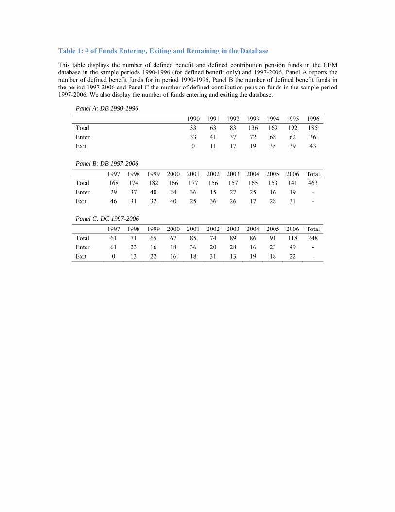
Table 1: # of Funds Entering, Exiting and Remaining in the Database

This table displays the number of defined benefit and defined contribution pension funds in the CEM database in the sample periods 1990-1996 (for defined benefit only) and 1997-2006. Panel A reports the number of defined benefit funds for in period 1990-1996, Panel B the number of defined benefit funds in the period 1997-2006 and Panel C the number of defined contribution pension funds in the sample period 1997-2006. We also display the number of funds entering and exiting the database.

Panel A: DB 1990-1996 1990 1991 1992 1993 1994 1995 1996

Total 33 63 83 136 169 192 185 Enter 33 41 37 72 68 62 36 Exit 0 11 17 19 35 39 43 Panel B: DB 1997-2006 1997 1998 1999 2000 2001 2002 2003 2004 2005 2006 Total Total 168 174 182 166 177 156 157 165 153 141 463 Enter 29 37 40 24 36 15 27 25 16 19 - Exit 46 31 32 40 25 36 26 17 28 31 - Panel C: DC 1997-2006 1997 1998 1999 2000 2001 2002 2003 2004 2005 2006 Total Total 61 71 65 67 85 74 89 86 91 118 248 Enter 61 23 16 18 36 20 28 16 23 49 - Exit 0 13 22 16 18 31 13 19 18 22 -

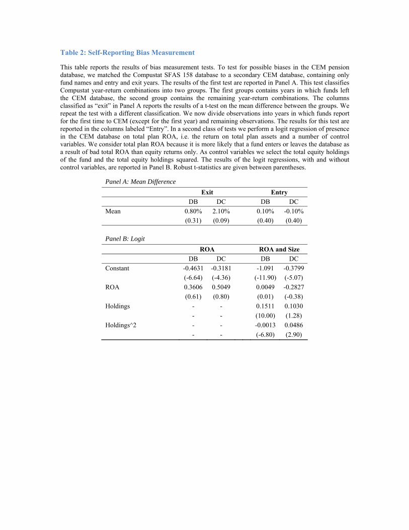
Table 2: Self-Reporting Bias Measurement

This table reports the results of bias measurement tests. To test for possible biases in the CEM pension database, we matched the Compustat SFAS 158 database to a secondary CEM database, containing only fund names and entry and exit years. The results of the first test are reported in Panel A. This test classifies Compustat year-return combinations into two groups. The first groups contains years in which funds left the CEM database, the second group contains the remaining year-return combinations. The columns classified as “exit” in Panel A reports the results of a t-test on the mean difference between the groups. We repeat the test with a different classification. We now divide observations into years in which funds report for the first time to CEM (except for the first year) and remaining observations. The results for this test are reported in the columns labeled “Entry”. In a second class of tests we perform a logit regression of presence in the CEM database on total plan ROA, i.e. the return on total plan assets and a number of control variables. We consider total plan ROA because it is more likely that a fund enters or leaves the database as a result of bad total ROA than equity returns only. As control variables we select the total equity holdings of the fund and the total equity holdings squared. The results of the logit regressions, with and without control variables, are reported in Panel B. Robust t-statistics are given between parentheses.

Panel A: Mean Difference Exit Entry DB DC DB DC Mean 0.80% 2.10% 0.10% -0.10% (0.31) (0.09) (0.40) (0.40) Panel B: Logit ROA ROA and Size DB DC DB DC Constant -0.4631 -0.3181 -1.091 -0.3799 (-6.64) (-4.36) (-11.90) (-5.07) ROA 0.3606 0.5049 0.0049 -0.2827 (0.61) (0.80) (0.01) (-0.38) Holdings - - 0.1511 0.1030 - - (10.00) (1.28) Holdings^2 - - -0.0013 0.0486 - - (-6.80) (2.90)

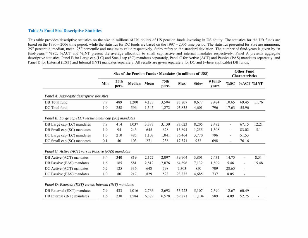
Table 3: Fund Size Descriptive Statistics

This table provides descriptive statistics on the size in millions of US dollars of US pension funds investing in US equity. The statistics for the DB funds are based on the 1990 – 2006 time period, while the statistics for DC funds are based on the 1997 – 2006 time period. The statistics presented for Size are minimum, 25th percentile, median, mean, 75th percentile and maximum value respectively. Stdev refers to the standard deviation. The number of fund-years is given by “# fund-years.” %SC, %ACT and %INT present the average allocation to small cap, active and internal mandates respectively. Panel A presents aggregate descriptive statistics, Panel B for Large cap (LC) and Small cap (SC) mandates separately, Panel C for Active (ACT) and Passive (PAS) mandates separately, and Panel D for External (EXT) and Internal (INT) mandates separately. All results are given separately for DC and (where applicable) DB funds.

Size of the Pension Funds / Mandates (in millions of US$) Other Fund Characteristics

Min 25th perc. Median Mean 75th

perc. Max Stdev # fund-years %SC %ACT %INT

Panel A: Aggregate descriptive statistics DB Total fund 7.9 489 1,200 4,173 3,504 83,807 8,677 2,484 10.65 69.45 11.76 DC Total fund 1.0 258 596 1,345 1,272 93,835 4,601 796 17.63 55.96 Panel B: Large cap (LC) versus Small cap (SC) mandates DB Large cap (LC) mandates 7.9 414 1,037 3,387 3,139 83,023 8,205 2,482 - 67.15 12.21 DB Small cap (SC) mandates 1.9 94 243 645 628 13,694 1,255 1,308 - 83.02 5.1 DC Large cap (LC) mandates 1.0 210 485 1,107 1,041 76,464 3,770 796 - 51.53 DC Small cap (SC) mandates 0.1 40 103 271 238 17,371 932 698 - 76.16 Panel C: Active (ACT) versus Passive (PAS) mandates DB Active (ACT) mandates 3.4 340 819 2,172 2,097 39,904 3,801 2,431 14.75 - 8.51 DB Passive (PAS) mandates 1.6 185 581 2,812 2,076 64,896 7,132 1,809 5.46 - 15.48 DC Active (ACT) mandates 5.2 125 336 648 798 7,303 850 709 28.65 - DC Passive (PAS) mandates 1.0 80 217 829 528 93,835 4,685 737 8.05 - Panel D: External (EXT) versus Internal (INT) mandates DB External (EXT) mandates 7.9 433 1,016 2,766 2,692 53,223 5,107 2,390 12.67 60.49 - DB Internal (INT) mandates 1.6 230 1,584 6,379 6,578 69,271 11,104 589 4.09 52.75 -

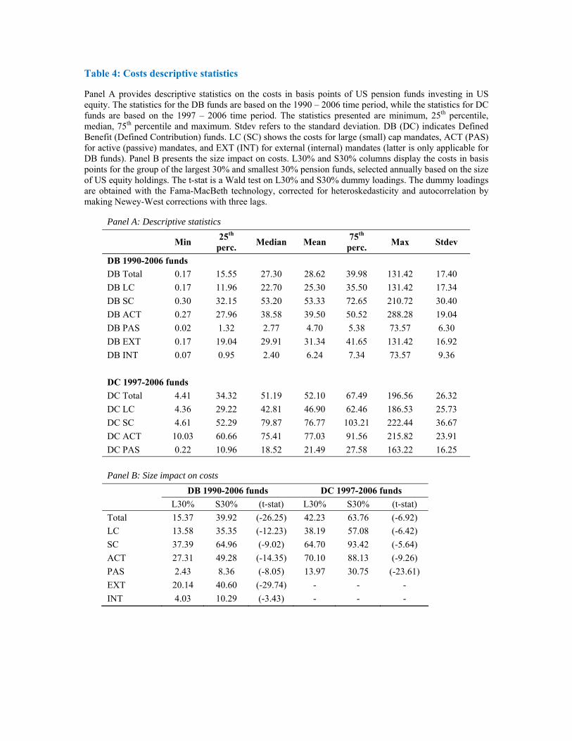
Table 4: Costs descriptive statistics

Panel A provides descriptive statistics on the costs in basis points of US pension funds investing in US equity. The statistics for the DB funds are based on the 1990 – 2006 time period, while the statistics for DC funds are based on the 1997 – 2006 time period. The statistics presented are minimum, 25th percentile, median, 75th percentile and maximum. Stdev refers to the standard deviation. DB (DC) indicates Defined Benefit (Defined Contribution) funds. LC (SC) shows the costs for large (small) cap mandates, ACT (PAS) for active (passive) mandates, and EXT (INT) for external (internal) mandates (latter is only applicable for DB funds). Panel B presents the size impact on costs. L30% and S30% columns display the costs in basis points for the group of the largest 30% and smallest 30% pension funds, selected annually based on the size of US equity holdings. The t-stat is a Wald test on L30% and S30% dummy loadings. The dummy loadings are obtained with the Fama-MacBeth technology, corrected for heteroskedasticity and autocorrelation by making Newey-West corrections with three lags.

Panel A: Descriptive statistics

Min 25th perc. Median Mean 75th

perc. Max Stdev

DB 1990-2006 funds DB Total 0.17 15.55 27.30 28.62 39.98 131.42 17.40 DB LC 0.17 11.96 22.70 25.30 35.50 131.42 17.34 DB SC 0.30 32.15 53.20 53.33 72.65 210.72 30.40 DB ACT 0.27 27.96 38.58 39.50 50.52 288.28 19.04 DB PAS 0.02 1.32 2.77 4.70 5.38 73.57 6.30 DB EXT 0.17 19.04 29.91 31.34 41.65 131.42 16.92 DB INT 0.07 0.95 2.40 6.24 7.34 73.57 9.36 DC 1997-2006 funds DC Total 4.41 34.32 51.19 52.10 67.49 196.56 26.32 DC LC 4.36 29.22 42.81 46.90 62.46 186.53 25.73 DC SC 4.61 52.29 79.87 76.77 103.21 222.44 36.67 DC ACT 10.03 60.66 75.41 77.03 91.56 215.82 23.91 DC PAS 0.22 10.96 18.52 21.49 27.58 163.22 16.25

Panel B: Size impact on costs

DB 1990-2006 funds DC 1997-2006 funds L30% S30% (t-stat) L30% S30% (t-stat)

Total 15.37 39.92 (-26.25) 42.23 63.76 (-6.92) LC 13.58 35.35 (-12.23) 38.19 57.08 (-6.42) SC 37.39 64.96 (-9.02) 64.70 93.42 (-5.64) ACT 27.31 49.28 (-14.35) 70.10 88.13 (-9.26) PAS 2.43 8.36 (-8.05) 13.97 30.75 (-23.61) EXT 20.14 40.60 (-29.74) - - - INT 4.03 10.29 (-3.43) - - -

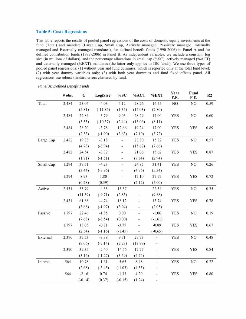
Table 5: Costs Regressions

This table reports the results of pooled panel regressions of the costs of domestic equity investments at the fund (Total) and mandate (Large Cap, Small Cap, Actively managed, Passively managed, Internally managed and Externally managed mandates), for defined benefit funds (1990-2006) in Panel A and for defined contribution funds (1997-2006) in Panel B. As independent variables, we include a constant, log size (in millions of dollars), and the percentage allocations in small cap (%SC), actively managed (%ACT) and externally managed (%EXT) mandates (the latter only applies to DB funds). We use three types of pooled panel regressions: (1) without year and fund dummies, which is reported only at the total fund level; (2) with year dummy variables only; (3) with both year dummies and fund fixed effects panel. All regressions use robust standard errors clustered by fund.

Panel A: Defined Benefit Funds

# obs. C Log(Size) %SC %ACT %EXT Year F.E.

Fund F.E. R2

Total 2,484 23.04 -4.03 4.12 28.26 16.55 NO NO 0.59 (5.81) (-11.85) (1.35) (15.03) (7.80) 2,484 22.84 -3.79 9.03 28.29 17.00 YES NO 0.60 (5.53) (-10.37) (2.44) (15.06) (8.11) 2,484 28.20 -3.78 12.66 19.24 17.00 YES YES 0.89 (2.33) (-1.90) (3.63) (7.10) (3.72) Large Cap 2,482 19.33 -3.18 - 28.80 15.82 YES NO 0.57 (4.73) (-8.94) - (15.62) (7.66) 2,482 24.54 -3.32 - 21.06 15.62 YES YES 0.87 (1.81) (-1.51) - (7.34) (2.94) Small Cap 1,294 39.51 -4.23 - 24.85 31.41 YES NO 0.26 (3.44) (-3.96) - (4.76) (5.34) 1,294 8.93 1.80 - 17.10 27.97 YES YES 0.72 (0.28) (0.39) - (2.12) (5.00) Active 2,431 53.79 -4.53 13.37 - 22.34 YES NO 0.35 (11.59) (-9.71) (2.83) - (9.88) 2,431 61.88 -4.74 18.12 - 13.74 YES YES 0.78 (3.68) (-1.97) (3.94) - (2.05) Passive 1,797 22.46 -1.85 0.00 - -1.06 YES NO 0.19 (7.68) (-8.54) (0.00) - (-1.61) 1,797 13.05 -0.81 -3.75 - -0.89 YES YES 0.67 (2.54) (-1.16) (-1.45) - (-0.65) External 2,390 37.53 -3.38 9.71 29.73 - YES NO 0.48 (9.06) (-7.14) (2.23) (13.99) - 2,390 39.35 -2.40 14.56 17.77 - YES YES 0.84 (3.16) (-1.27) (3.59) (4.74) - Internal 564 10.78 -1.61 -5.65 8.48 - YES NO 0.22 (2.68) (-3.45) (-1.03) (4.35) - 564 -2.16 0.74 -1.33 4.20 - YES YES 0.80 (-0.14) (0.37) (-0.15) (1.24) -

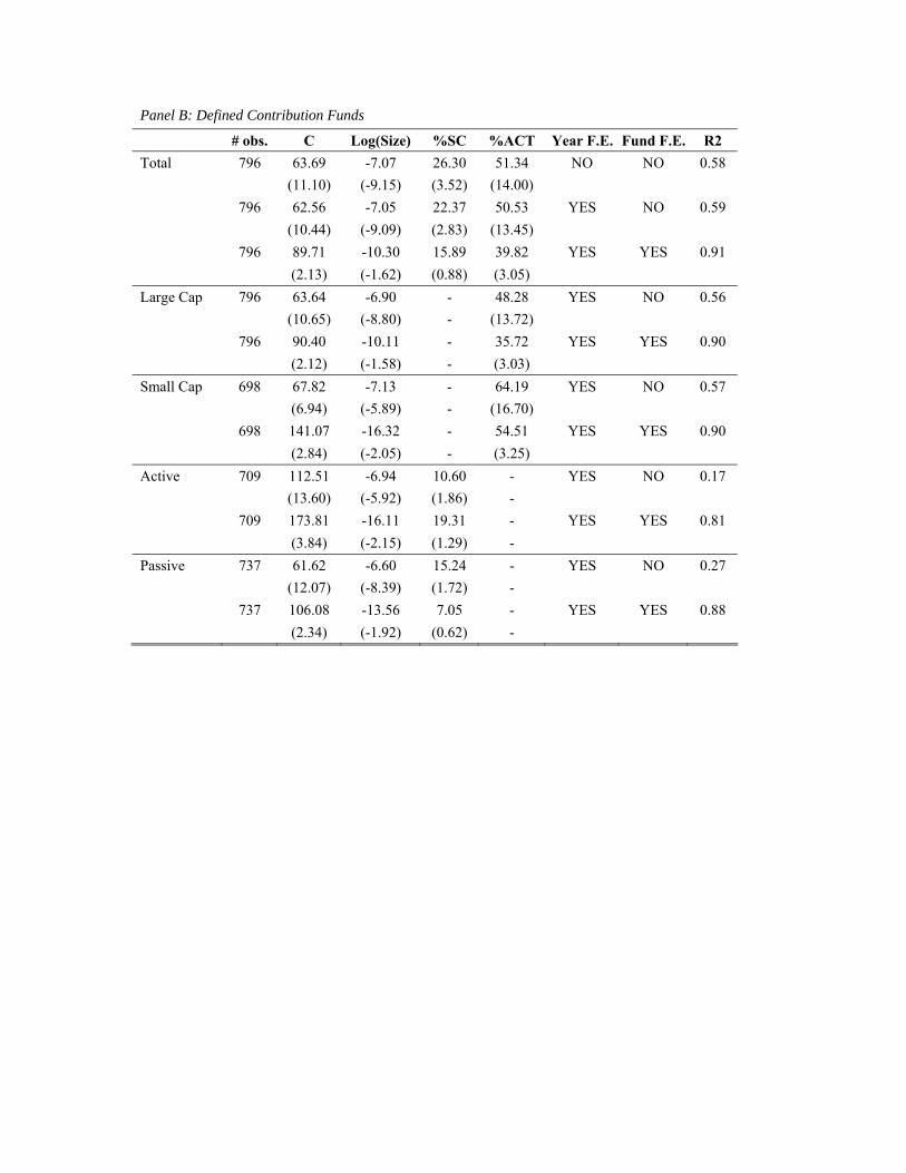
Panel B: Defined Contribution Funds

# obs. C Log(Size) %SC %ACT Year F.E. Fund F.E. R2 Total 796 63.69 -7.07 26.30 51.34 NO NO 0.58 (11.10) (-9.15) (3.52) (14.00) 796 62.56 -7.05 22.37 50.53 YES NO 0.59 (10.44) (-9.09) (2.83) (13.45) 796 89.71 -10.30 15.89 39.82 YES YES 0.91 (2.13) (-1.62) (0.88) (3.05) Large Cap 796 63.64 -6.90 - 48.28 YES NO 0.56 (10.65) (-8.80) - (13.72) 796 90.40 -10.11 - 35.72 YES YES 0.90 (2.12) (-1.58) - (3.03) Small Cap 698 67.82 -7.13 - 64.19 YES NO 0.57 (6.94) (-5.89) - (16.70) 698 141.07 -16.32 - 54.51 YES YES 0.90 (2.84) (-2.05) - (3.25) Active 709 112.51 -6.94 10.60 - YES NO 0.17 (13.60) (-5.92) (1.86) - 709 173.81 -16.11 19.31 - YES YES 0.81 (3.84) (-2.15) (1.29) - Passive 737 61.62 -6.60 15.24 - YES NO 0.27 (12.07) (-8.39) (1.72) - 737 106.08 -13.56 7.05 - YES YES 0.88 (2.34) (-1.92) (0.62) -

Table 6: Net Risk-adjusted Performance at the Fund Level

This table reports the risk-adjusted performance of pension funds at the fund level. To risk-adjust, we use the four-factor Fama-French-Carhart model, and the random coefficient model as described in Section 3. We report the annual alpha as well as the betas on the Market, Size, Book-to-Market and Momentum factors. In Panel A (B), we use the total net (of all costs) excess return and net benchmark-adjusted return of defined benefit (contribution) pension plans. For defined benefit pension funds the data period is 1990-2006 and for defined contribution funds 1997-2006. RMSE is the root mean squared error. Robust t-stats are in parentheses.

Panel A: Defined Benefit Total Net Returns α RMSE

Net Returns 0.0132 0.9012 -0.0092 -0.0166 -0.0898 0.0901 (4.93) (79.64) (-0.33) (-0.73) (-4.38)

Benchmark-adj. 0.0045 -0.0489 0.0348 -0.0178 -0.0152 0.0783 Net Returns (1.82) (-5.10) (1.43) (-0.93) (-0.84) Panel B: Defined Contribution Total Net Returns

α RMSE Net Returns 0.0140 0.9775 -0.0555 -0.0966 -0.1004 0.0479

(2.74) (62.90) (-3.43) (-2.14) (-2.93) Benchmark-adj. 0.0083 -0.0381 0.0037 -0.1029 -0.0631 0.0412 Net Returns (1.52) (-2.62) (2.26) (-2.45) (-1.93)

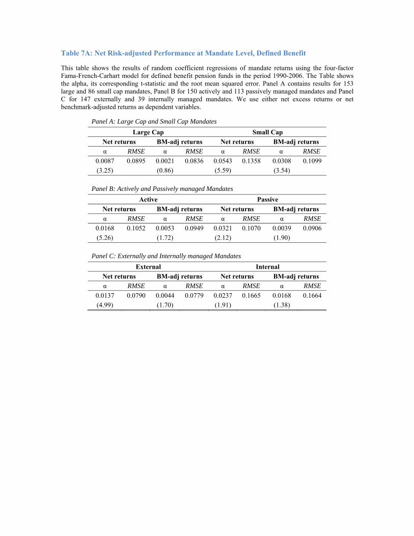
Table 7A: Net Risk-adjusted Performance at Mandate Level, Defined Benefit

This table shows the results of random coefficient regressions of mandate returns using the four-factor Fama-French-Carhart model for defined benefit pension funds in the period 1990-2006. The Table shows the alpha, its corresponding t-statistic and the root mean squared error. Panel A contains results for 153 large and 86 small cap mandates, Panel B for 150 actively and 113 passively managed mandates and Panel C for 147 externally and 39 internally managed mandates. We use either net excess returns or net benchmark-adjusted returns as dependent variables.

Panel A: Large Cap and Small Cap Mandates Large Cap Small Cap

Net returns BM-adj returns Net returns BM-adj returns α RMSE α RMSE α RMSE α RMSE

0.0087 0.0895 0.0021 0.0836 0.0543 0.1358 0.0308 0.1099 (3.25) (0.86) (5.59) (3.54)

Panel B: Actively and Passively managed Mandates

Active Passive Net returns BM-adj returns Net returns BM-adj returns α RMSE α RMSE α RMSE α RMSE

0.0168 0.1052 0.0053 0.0949 0.0321 0.1070 0.0039 0.0906 (5.26) (1.72) (2.12) (1.90)

Panel C: Externally and Internally managed Mandates

External Internal Net returns BM-adj returns Net returns BM-adj returns α RMSE α RMSE α RMSE α RMSE

0.0137 0.0790 0.0044 0.0779 0.0237 0.1665 0.0168 0.1664 (4.99) (1.70) (1.91) (1.38)

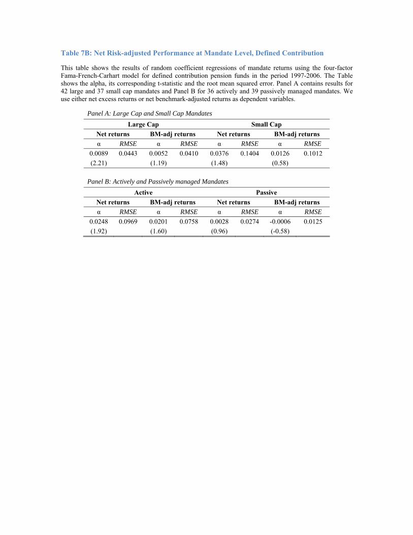
Table 7B: Net Risk-adjusted Performance at Mandate Level, Defined Contribution

This table shows the results of random coefficient regressions of mandate returns using the four-factor Fama-French-Carhart model for defined contribution pension funds in the period 1997-2006. The Table shows the alpha, its corresponding t-statistic and the root mean squared error. Panel A contains results for 42 large and 37 small cap mandates and Panel B for 36 actively and 39 passively managed mandates. We use either net excess returns or net benchmark-adjusted returns as dependent variables.

Panel A: Large Cap and Small Cap Mandates Large Cap Small Cap

Net returns BM-adj returns Net returns BM-adj returns α RMSE α RMSE α RMSE α RMSE

0.0089 0.0443 0.0052 0.0410 0.0376 0.1404 0.0126 0.1012 (2.21) (1.19) (1.48) (0.58)

Panel B: Actively and Passively managed Mandates

Active Passive Net returns BM-adj returns Net returns BM-adj returns α RMSE α RMSE α RMSE α RMSE

0.0248 0.0969 0.0201 0.0758 0.0028 0.0274 -0.0006 0.0125 (1.92) (1.60) (0.96) (-0.58)

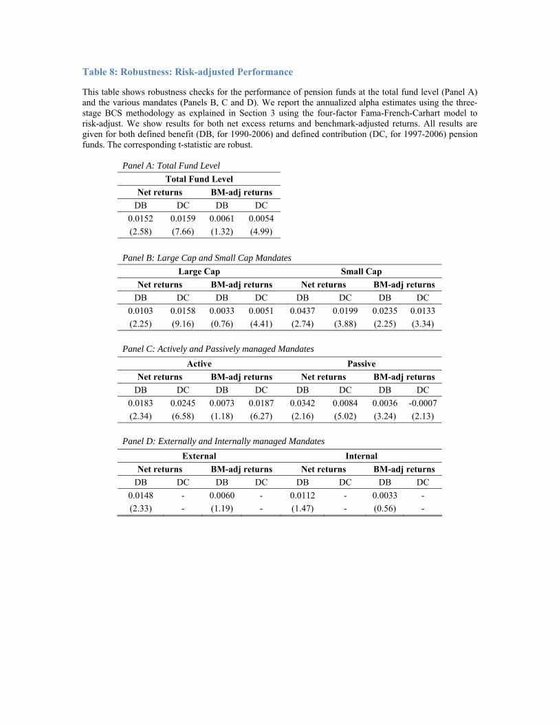
Table 8: Robustness: Risk-adjusted Performance

This table shows robustness checks for the performance of pension funds at the total fund level (Panel A) and the various mandates (Panels B, C and D). We report the annualized alpha estimates using the three-stage BCS methodology as explained in Section 3 using the four-factor Fama-French-Carhart model to risk-adjust. We show results for both net excess returns and benchmark-adjusted returns. All results are given for both defined benefit (DB, for 1990-2006) and defined contribution (DC, for 1997-2006) pension funds. The corresponding t-statistic are robust.

Panel A: Total Fund Level Total Fund Level

Net returns BM-adj returns DB DC DB DC

0.0152 0.0159 0.0061 0.0054 (2.58) (7.66) (1.32) (4.99)

Panel B: Large Cap and Small Cap Mandates

Large Cap Small Cap Net returns BM-adj returns Net returns BM-adj returns

DB DC DB DC DB DC DB DC 0.0103 0.0158 0.0033 0.0051 0.0437 0.0199 0.0235 0.0133 (2.25) (9.16) (0.76) (4.41) (2.74) (3.88) (2.25) (3.34)

Panel C: Actively and Passively managed Mandates

Active Passive Net returns BM-adj returns Net returns BM-adj returns

DB DC DB DC DB DC DB DC 0.0183 0.0245 0.0073 0.0187 0.0342 0.0084 0.0036 -0.0007 (2.34) (6.58) (1.18) (6.27) (2.16) (5.02) (3.24) (2.13)

Panel D: Externally and Internally managed Mandates

External Internal Net returns BM-adj returns Net returns BM-adj returns

DB DC DB DC DB DC DB DC 0.0148 - 0.0060 - 0.0112 - 0.0033 - (2.33) - (1.19) - (1.47) - (0.56) -

Table 9: Liquidity Betas and Performance

This table shows the results of a random coefficient regression of total net domestic equity returns on the excess return on a five-factor model that includes the market, size, value and momentum of the Fama-French-Carhart model appended with the Pastor and Stambaugh (2003) traded liquidity factor. We only show the liquidity beta. We display the parameter estimates (with corresponding t-statistics in parentheses) and the root mean squared error for net returns on total domestic equity returns. We show results for defined benefit funds (1990-2006) and for defined contribution funds (1997-2006), and for net domestic equity returns at the total fund level and the various mandate levels: large and small cap mandates, actively and passively managed mandates and externally and internally managed mandates.

Defined Benefit Defined Contribution α RMSE α RMSE

Total 0.0194 -0.0883 0.0768 0.0241 -0.0576 0.0400 (6.78) (-5.27) (4.79) (-2.12) Large Cap 0.0124 -0.0505 0.0756 0.0150 0.0005 0.0349 (4.17) (-2.89) (2.90) (0.02) Small Cap 0.0633 -0.3995 0.1021 0.0342 -0.3950 0.0925 (6.67) (-9.87) (0.69) (-2.71) Active 0.0238 -0.1259 0.0897 0.0528 -0.1806 0.0724 (7.20) (-6.16) (4.33) (-3.06) Passive 0.0203 -0.2861 0.0746 0.0012 0.0499 0.0217 (1.43) (-2.21) (0.53) (3.39) External 0.0203 -0.0974 0.0788 - - - (6.70) (-5.67) - - Internal 0.0217 -0.0638 0.1627 - - - (2.39) (-1.88) - -

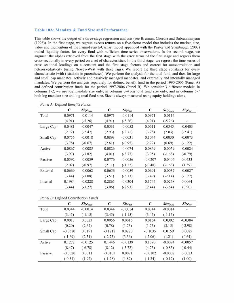
Table 10A: Mandate & Fund Size and Performance

This table shows the output of a three-stage regression analysis (see Brennan, Chordia and Subrahmanyam (1998)). In the first stage, we regress excess returns on a five-factor model that includes the market, size, value and momentum of the Fama-French-Carhart model appended with the Pastor and Stambaugh (2003) traded liquidity factor. for every fund with sufficient time series observations. In the second stage, we augment the alphas retrieved from the first stage with the error terms of the first stage and regress them cross-sectionally in every period on a set of characteristics. In the third stage, we regress the time series of cross-sectional loadings on a constant and the first stage factors and correct for autocorrelation and heteroskedasticity (using Newey-West with three lags). We report the third stage constants for every characteristic (with t-statistic in parentheses). We perform the analysis for the total fund, and then for large and small cap mandates, actively and passively managed mandates, and externally and internally managed mandates. We perform the analysis separately for defined benefit fund in the period 1990-2006 (Panel A) and defined contribution funds for the period 1997-2006 (Panel B). We consider 3 different models: in columns 1-2, we use log mandate size only, in columns 3-4 log total fund size only, and in columns 5-7 both log mandate size and log total fund size. Size is always measured using equity holdings alone.

Panel A: Defined Benefits Funds C Sizeman C Sizetot C Sizeman Sizetot

Total 0.0971 -0.0114 0.0971 -0.0114 0.0971 -0.0114 - (4.91) (-5.26) (4.91) (-5.26) (4.91) (-5.26) - Large Cap 0.0481 -0.0047 0.0531 -0.0052 0.0611 0.0345 -0.0403 (2.72) (-2.47) (2.93) (-2.71) (3.28) (2.03) (-2.41) Small Cap 0.0756 -0.0018 0.0893 -0.0031 0.1044 0.0030 -0.0073 (3.78) (-0.67) (2.61) (-0.95) (2.72) (0.69) (-1.22) Active 0.0867 -0.0085 0.0826 -0.0074 0.0869 -0.0059 -0.0024 (3.97) (-3.82) (4.01) (-3.77) (3.95) (-1.68) (-0.79) Passive 0.0592 -0.0039 0.0776 -0.0056 -0.0207 -0.0406 0.0433 (2.02) (-0.97) (2.11) (-1.22) (-0.48) (-1.63) (1.59) External 0.0669 -0.0062 0.0656 -0.0059 0.0691 -0.0037 -0.0027 (3.44) (-3.08) (3.51) (-3.13) (3.49) (-2.14) (-1.77) Internal 0.1984 -0.0228 0.2865 -0.0304 0.1744 -0.0268 0.0064 (3.44) (-3.27) (3.06) (-2.93) (2.44) (-3.64) (0.90)

Panel B: Defined Contribution Funds

C Sizeman C Sizetot C Sizeman Sizetot

Total 0.0344 -0.0014 0.0344 -0.0014 0.0344 -0.0014 - (3.45) (-1.15) (3.45) (-1.15) (3.45) (-1.15) - Large Cap 0.0013 0.0023 0.0056 0.0016 0.0154 0.0392 -0.0384 (0.20) (2.62) (0.78) (1.73) (1.75) (3.15) (-2.98) Small Cap -0.0580 0.0191 -0.1218 0.0220 -0.1035 0.0159 0.0085 (-1.69) (2.51) (-2.73) (3.56) (-2.06) (1.21) (0.64) Active 0.1272 -0.0125 0.1446 -0.0139 0.1390 -0.0084 -0.0057 (8.47) (-6.78) (8.12) (-5.72) (4.75) (-0.85) (-0.44) Passive -0.0020 0.0011 -0.0103 0.0021 -0.0102 -0.0002 0.0023 (-0.54) (1.92) (-1.28) (1.87) (-1.24) (-0.12) (1.00)

Table 10B: Mandate Size, Liquidity and Performance

This table shows the output of a three-stage regression analysis (see Brennan, Chordia and Subrahmanyam (1998)), see Table 10A for a description. We perform the analysis separately for defined benefit fund in the period 1990-2006 (Panel A) and defined contribution funds for the period 1997-2006 (Panel B). We select a constant, log mandate size and the interaction of log mandate size with the first stage fund-specific loading on the liquidity factor as characteristics. The final column reports the cross-sectional correlation between log mandate size and its interaction with the first stage fund-specific loading on the liquidity factor. Size is always measured using equity holdings alone.

Panel A: Defined Benefit C Sizeman Sizeman*βLiq ρ

Total 0.0686 -0.0087 -0.0104 0.3103 (3.78) (-4.49) (-3.34) Large Cap 0.0254 -0.0022 -0.0144 0.2574 (2.00) (-1.73) (-4.30) Small Cap 0.0241 -0.0006 -0.0217 0.1915 (0.45) (-0.08) (-3.47) Active 0.0600 -0.0060 -0.0089 0.2746 (3.13) (-3.05) (-2.86) Passive -0.0662 0.0089 -0.0259 0.1130 (-0.72) (0.91) (-1.63) External 0.0439 -0.0043 -0.0123 0.2003 (2.66) (-2.50) (-4.35) Internal 0.0656 -0.0069 -0.0268 0.3911 (2.53) (-2.20) (-5.61)

Panel B: Defined Contribution

C Sizeman Sizeman*βLiq ρ

Total 0.0354 -0.0024 -0.0141 -0.1571 (2.85) (-1.47) (-11.38) Large Cap 0.0148 0.0001 -0.0164 -0.1970 (1.78) (0.06) (-11.41) Small Cap -0.0763 0.0141 -0.0323 -0.2291 (-2.16) (1.63) (-3.92) Active 0.0992 -0.0116 -0.0237 0.0938 (8.26) (-6.96) (-9.31) Passive -0.0004 0.0011 -0.0047 -0.4107 (-0.08) (1.58) (-1.60)

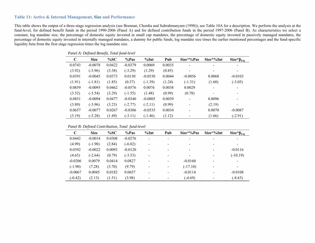
Table 11: Active & Internal Management, Size and Performance

This table shows the output of a three-stage regression analysis (see Brennan, Chordia and Subrahmanyam (1998)), see Table 10A for a description. We perform the analysis at the fund-level, for defined benefit funds in the period 1990-2006 (Panel A) and for defined contribution funds in the period 1997-2006 (Panel B). As characteristics we select a constant, log mandate size, the percentage of domestic equity invested in small cap mandates, the percentage of domestic equity invested in passively managed mandates, the percentage of domestic equity invested in internally managed mandates, a dummy for public funds, log mandate size times the earlier mentioned percentages and the fund-specific liquidity beta from the first stage regression times the log mandate size.

Panel A: Defined Benefit, Total fund-level C Size %SC %Pas %Int Pub Size*%Pas Size*%Int Size*βLiq

0.0743 -0.0078 0.0422 -0.0379 0.0069 0.0035 - - - (3.92) (-3.96) (3.38) (-3.29) (1.29) (0.85) - - - 0.0391 -0.0045 0.0373 0.0150 -0.0530 0.0044 -0.0056 0.0068 -0.0103 (1.91) (-1.81) (1.85) (0.37) (-1.39) (1.24) (-1.31) (1.60) (-3.05) 0.0859 -0.0095 0.0462 -0.0576 0.0076 0.0038 0.0029 - - (3.52) (-3.54) (3.29) (-1.55) (1.48) (0.99) (0.78) - - 0.0851 -0.0094 0.0477 -0.0340 -0.0805 0.0039 - 0.0096 - (3.89) (-3.96) (3.23) (-2.77) (-2.11) (0.99) - (2.19) - 0.0657 -0.0077 0.0267 -0.0306 -0.0535 0.0034 - 0.0070 -0.0087 (3.19) (-3.28) (1.49) (-3.11) (-1.46) (1.12) - (1.66) (-2.91)

Panel B: Defined Contribution, Total fund-level

C Size %SC %Pas %Int Pub Size*%Pas Size*%Int Size*βLiq

0.0442 -0.0014 0.0308 -0.0276 - - - - - (4.99) (-1.90) (2.84) (-6.02) - - - - - 0.0392 -0.0022 0.0093 -0.0120 - - - - -0.0116 (4.65) (-2.64) (0.79) (-3.53) - - - - (-10.19)

-0.0206 0.0079 0.0414 0.0827 - - -0.0160 - - (-1.90) (7.28) (3.70) (9.79) - - (-17.10) - - -0.0067 0.0045 0.0182 0.0657 - - -0.0114 - -0.0108 (-0.42) (2.13) (1.51) (3.98) - - (-4.69) - (-8.63)

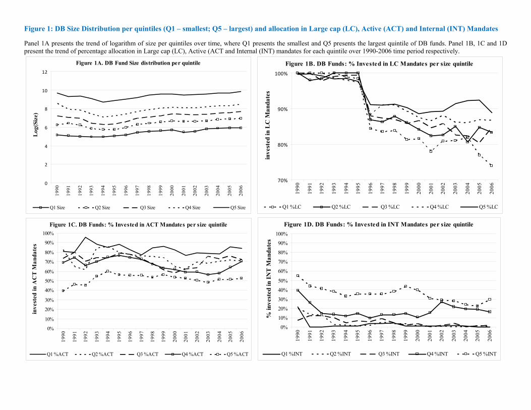
Figure 1: DB Size Distribution per quintiles (Q1 – smallest; Q5 – largest) and allocation in Large cap (LC), Active (ACT) and Internal (INT) Mandates

Panel 1A presents the trend of logarithm of size per quintiles over time, where Q1 presents the smallest and Q5 presents the largest quintile of DB funds. Panel 1B, 1C and 1D present the trend of percentage allocation in Large cap (LC), Active (ACT and Internal (INT) mandates for each quintile over 1990-2006 time period respectively.

Figure 1A. DB Fund Size distribution per quintile

0

2

4

6

8

10

12

1990

1991

1992

1993

1994

1995

1996

1997

1998

1999

2000

2001

2002

2003

2004

2005

2006

Log

(Siz

e)

Q1 Size Q2 Size Q3 Size Q4 Size Q5 Size 

Figure 1B. DB Funds: % Invested in LC Mandates per size quintile

70%

80%

90%

100%

1990

1991

1992

1993

1994

1995

1996

1997

1998

1999

2000

2001

2002

2003

2004

2005

2006

inve

sted

in L

C M

anda

tes

Q1 %LC Q2 %LC Q3 %LC Q4 %LC Q5 %LC 

Figure 1C. DB Funds: % Invested in ACT Mandates per size quintile

0%

10%

20%

30%

40%

50%

60%

70%

80%

90%

100%

1990

1991

1992

1993

1994

1995

1996

1997

1998

1999

2000

2001

2002

2003

2004

2005

2006

inve

sted

in A

CT

Man

date

s

Q1 %ACT Q2 %ACT Q3 %ACT Q4 %ACT Q5 %ACT 

Figure 1D. DB Funds: % Invested in INT Mandates per size quintile

0%

10%

20%

30%

40%

50%

60%

70%

80%

90%

100%

1990

1991

1992

1993

1994

1995

1996

1997

1998

1999

2000

2001

2002

2003

2004

2005

2006

% in

vest

ed in

IN

T M

anda

tes

Q1 %INT Q2 %INT Q3 %INT Q4 %INT Q5 %INT 

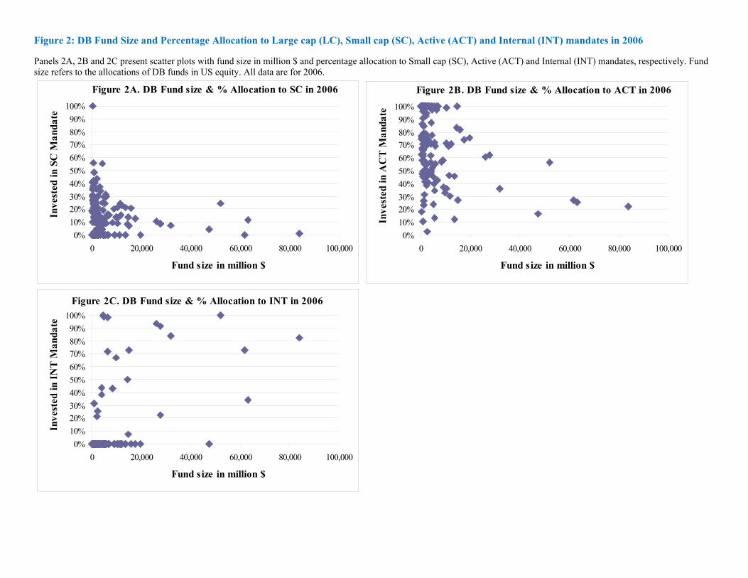
Figure 2: DB Fund Size and Percentage Allocation to Large cap (LC), Small cap (SC), Active (ACT) and Internal (INT) mandates in 2006

Panels 2A, 2B and 2C present scatter plots with fund size in million $ and percentage allocation to Small cap (SC), Active (ACT) and Internal (INT) mandates, respectively. Fund size refers to the allocations of DB funds in US equity. All data are for 2006.

Figure 2A. DB Fund size & % Allocation to SC in 2006

0%10%20%30%40%50%60%70%80%90%

100%

0 20,000 40,000 60,000 80,000 100,000

Fund size in million $

Inve

sted

in S

C M

anda

te

Figure 2B. DB Fund size & % Allocation to ACT in 2006

0%10%20%30%40%50%60%70%80%90%

100%

0 20,000 40,000 60,000 80,000 100,000

Fund size in million $

Inve

sted

in A

CT

Man

date

 Figure 2C. DB Fund size & % Allocation to INT in 2006

0%10%20%30%40%50%60%70%80%90%

100%

0 20,000 40,000 60,000 80,000 100,000

Fund size in million $

Inve

sted

in I

NT

Man

date

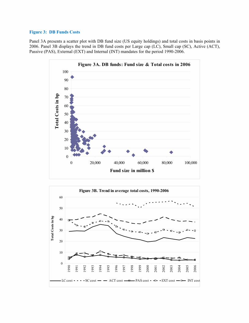
Figure 3: DB Funds Costs

Panel 3A presents a scatter plot with DB fund size (US equity holdings) and total costs in basis points in 2006. Panel 3B displays the trend in DB fund costs per Large cap (LC), Small cap (SC), Active (ACT), Passive (PAS), External (EXT) and Internal (INT) mandates for the period 1990-2006.

Figure 3A. DB funds: Fund size & Total costs in 2006

0

10

20

30

40

50

60

70

80

90

100

0 20,000 40,000 60,000 80,000 100,000

Fund size in million $

Tot

al C

osts

in b

p

 

Figure 3B. Trend in average total costs, 1990-2006

0

10

20

30

40

50

60

1990

1991

1992

1993

1994

1995

1996

1997

1998

1999

2000

2001

2002

2003

2004

2005

2006

Tot

al C

osts

in b

p

LC cost SC cost ACT cost PAS cost EXT cost INT cost

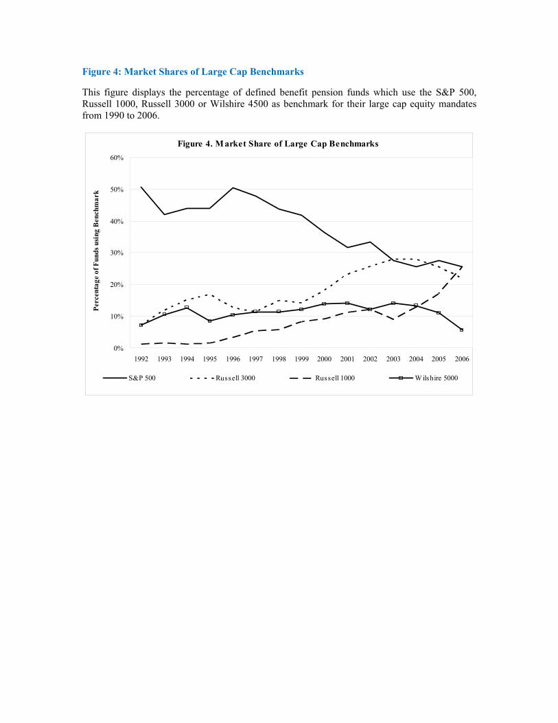
Figure 4: Market Shares of Large Cap Benchmarks

This figure displays the percentage of defined benefit pension funds which use the S&P 500, Russell 1000, Russell 3000 or Wilshire 4500 as benchmark for their large cap equity mandates from 1990 to 2006.

Figure 4. M arket Share of Large Cap Benchmarks

0%

10%

20%

30%

40%

50%

60%

1992 1993 1994 1995 1996 1997 1998 1999 2000 2001 2002 2003 2004 2005 2006

Perc

enta

ge o

f Fun

ds u

sing

Ben

chm

ark

S&P 500 Russell 3000 Russell 1000 W ilshire 5000

46

Figure 5: Market Share of Small Cap Benchmarks

This figure displays the percentage of defined benefit pension funds which use the Russell 2000, Russell 2500, Russell 3000, Wilshire 4500, Wilshire 5000, S&P 400, S&P 500 or S&P 600 as benchmark for their small cap equity mandates from 1990 to 2006.

Figure 5. Market Share of Small Cap Benchmarks

0%

10%

20%

30%

40%

50%

60%

1992 1993 1994 1995 1996 1997 1998 1999 2000 2001 2002 2003 2004 2005 2006

Perc

enta

ge o

f Fun

ds u

sing

Ben

chm

ark

Russell 2000

Russell 2500

Russell 3000

W ilshire4500

W ilshire5000S&P 400

S&P 500

S&P 600