NBER WORKING PAPER SERIES

GLOBAL REAL ESTATE MARKETS -CYCLES AND FUNDAMENTALS

Bradford CaseWilliam N. GoetzmannK. Geert Rouwenhorst

Working Paper 7566http://www.nber.org/papers/w7566

NATIONAL BUREAU OF ECONOMIC RESEARCH1050 Massachusetts Avenue

Cambridge, MA 02138February 2000

We thanklbbotson Associates and members of the International Commercial Property Associates consortiumfor use of their data. We thank the International Center for Finance at the Yale School of Management forresearch support. The views expressed herein are those of the authors and are not necessarily those of theNational Bureau of Economic Research.

2000 by Bradford Case, William N. Goetzmann, and K. Geert Rouwenhorsi. All rights reserved. Shortsections of text, not to exceed two paragraphs, may be quoted without explicit permission provided that fullcredit, including notice, is given to the source.

Global Real Estate Markets — Cycles and FundamentalsBradford Case, William Goetzmann, and K. Geert RouwenhorstNBER Working Paper No. 7566February 2000

ABSTRACT

The correlations among international real estate markets are surprisingly high, given the

degree to which they are segmented. While industrial, office and retail properties exist all around the

world, they are not economic substitutes because of locational specificity. In addition, the broad

securitization of real estate property companies has, until recently, lagged that of other types of

companies. Never-the-less, international property returns move together in dramatic fashion. In this

paper, we use eleven years of global property returns to explore the factors influencing this co-

movement. We attribute a substantial amount of the correlation across world property markets to

the effects of changes in GNP, suggesting that real estate is a bet on fundamental economic variables

which are correlated across countries. A decomposition shows that a local production factor is more

important in some countries than in others.

Bradford Case William N. GoetzmannYale University Yale School of ManagementNew Haven, CT 06520-8200 Box 208200

New Haven, CT 06520-8200and NBER

william.goetzmann@yale.edu

K. Geert RouwenhorstYale School of ManagementNew Haven, CT 06520-8200

I. Introduction

The real estate business is distinguished from almost all others by the fact that its "product"

is not portable. For the most part, property owners compete locally for business. While inter-urban

competition for industrial, office or retail space exists, customer choice depends upon a number of

economic factors beyond the price and quality of the space. Thus, one would expect the correlation

of changes in property values across markets to diminish with the distance between them. There

are no short-term arbitrage forces preventing prices in one local market from suddenly getting hot

while prices in another local market are dropping--buildings from one market cannot be moved to

the other. For the same reasons, one might also expect international property markets to exhibit

low correlations due to the difficulties of re-locating businesses across national boundaries. Studies

measuring the diversification benefits of real estate and other asset classes suggest real estate

compares favorably in this dimension (e.g. Eicholtz. 1996. Eicholtz and Hartzell, 1996. Eicholtz et.

Al, 1998, Liu and Mci, 1998, Liu, Hartzell and Hoeseli, 1997). After looking at recent published

empirical evidence, it is clear that international real estate investment is useful for portfolio

diversification.

This logic makes the evidence about co-movement in intemational property returns all the

more striking. Goetzmann and Wachter (1996) [OW] document that the real estate crash in the early

1990's was feitby nearly every country in the world. Despite their separation by political boundaries

and great distances, the world's office markets plunged into a slump together. While economists

looked for local reasons for local decreases in property values, the reality is that there were no safe

havens for property investors in the years 1991 and 1992. Diversification did not help. The

conjecture in GW was that this slump was due to exposures to global GDP. Unfortunately,

2

insufficient time-series data prevented any formal test of the conjecture. Work by Quan and Titman

(1998), using the same data sources as GW and longer time series document that real estate is

significantly correlated to stock returns and to changes in GDP. In his in-depth analysis of the

international real estate slump of the 1990's, Renaud (1997) considers the degree to which unique

events in the late 1980's may have led to the correlated change in real estate prices and the global

economy. He also discusses the co-cyclycality of global economies and real estate. Together, these

recent studies suggest that a mix of global and local economic factors influence the world's real

estate markets.

In this paper, we use 11 years of commercial property data to examine the relationship

between GNP changes property returns. We explore the relationship in considerably more depth

than OW and take a different approach to GDP effects than Quan and Titman. Our goal is to separate

global from local economic effects on the covariance of real estate returns. In particular, we test to

see whether the correlations across global real estate markets are due to common exposures to

changes in world GDP. In addition, we estimate the incremental value of local economic

fluctuations in explaining real estate performance. We find strong evidence to show that removing

the effects of both country-specific GDP and global GDP from returns significantly decreases global

real estate market correlations. Of the two, global GDP has the greatest effect.

The implications of our results are twofold. First, world real estate markets are largely

correlated through common GDP effects. Thus, we find that even markets that are segmented by

definition can exhibit significant correlations if they are exposed to a common source of risk.

Second, we show that an investment in a global real estate portfolio is essentially a bet on broad

trends in global production.

3

II. Data

International property return data is difficult to obtain. Some authors have collected returns

from publically traded property companies in a number of countries for successful analysis. This

is useful but not always representative of the markets in all countries, and depends upon the

existence of public markets in property companies. Our data source is a recently dissolved global

consortium of real estate firms that collectively shared yield and effective rent data sampled and

assembled on an annual basis. Until recently, these firms were affiliated through International

Commercial Property Associates (ICPA), with a successor agreement with ONCOR International.

Over the past decade, their estimates of yields and effective rents were formed by firms operating

in each market according to commonly agreed upon standards. These estimates were published as

ICPA's "International Property Bulletin" and ONCOR's "World Real Estate Review," and "European

Property Bulletin." Both ICPA and ONCOR have ceased publishing these data, but London-based

Hillier Parker has continued to organize European firms to share data for European markets. In

addition, the data for Asian real estate markets is also collected by several affiliates of Hillier Parker

and published by its Hong Kong affiliate. Brooke Hillier Parker, in "Asian Property Market Survey."

Throughout the time ICPA existed, new markets entered --particularly emerging markets in Asia.

The existence of these markets in the database is undoubtably conditioned upon investor interest,

and thus potentially biased by positive performance. Thus, some of the markets included in our

database may have been "backfilled" and the paucity of data about other markets, particularly the

lack of industrial and retail information about Japan, for example, may result from recent lack of

interest in international investing there.

Since we do not have income and capital appreciation returns reported as such in the

4

database, we estimate them using yields and cap-rates. Specifically, total returns (income and

appreciation) for prime industrial, office, and retail real estate in 22 cities around the world is the

sum of the estimated yield and the change in capitalized estimated effective rents:

= + _______ - I where T1, equals estimated total return for city i at time I; i,r

equals the estimated yields (going-in cap rates); and R1 equals estimated effective rents. This

implicitly assum.es that the perpetuity formula is a reasonable approximation to value. Rents and

yields were estimated for consistently-defined standard properties in the prime commercial districts

of each city by commercial real estate firms in each country.

While these sources present data for a large number of cities, the analysis must be restricted

to those markets for which estimated rents and yields are available for every year during the period

1987-1997. Table 1 shows the 22 markets from 21 countries included in the analysis under this

criterion. Two German markets, Dusseldorf and Frankfurt, are inc]uded. because the required data

were available for both cities.

While the effective rent data are given in nominal terms and generally denominated in local

currency, from the perspective of a U.S. investor it is more relevant to consider returns expressed

in U.S. dollars. Therefore the nominal foreign-currency returns were converted to real U.S. dollar

terms by using the exchange rate in effect at the end of each year and then deflating by the U.S.

inflation rate.

Table I shows the geometric means, arithmetic means, and standard deviations of the total

5

return series computed for each type of real estate, and for the stock market total return series. The

average total returns are in some cases spectacu]arly high: for example, the geometric means for the

11-year period exceed 20 percent for industrial space and office space in Hong Kong, Portugal,

Singapore, and Thailand and for retail space in Portugal and Thailand. At the same time, these

investments were extremely volatile, with standard deviations exceeding 40 percent in several cases.

The volatility for the U.S. is only slightly higher than obtained from other appraisal-based indices.

As a check on whether the yield-based return series' for the U.S. correspond to appraisal-

based returns in the U.S. we measured the correlation to the NCREIIF index . The U.S. Industrial

property index had a correlation of .84 to the NCREIF index and the U.S. Office property index had

a correlation of .56. Neither had a significant correlation to the NARE1T index of equity real estate

investment trusts. Thus, we are using series' that more closely resemble and indeed track the

appraisal-based indices commonly used in the U.S to measure commercial real estate performance.

Figure 1 shows the trend in real estate returns over the period 1987 through 1997 for each

country and property type. The crash of the early 1991 through 1993 shows up clearly as a majority

of markets and property types experiences negative real returns during the period. There were almost

no safe havens during this period. Only Hong Kong, Singapore, Malaysia and Portugal had strong

positive returns in the three-year slump. The year 1997 closely resembles the early 90's, when most

real returns were negative. The comovement between markets also shows up in the correlations.

We do not report the entire 60 by 60 correlation matrix, however, on average, the correlations within

property types across countries ranged between 0.33 and 0.44.

Figure 2 shows the dollar-denominated changes in GDP for each country, deflated by the

U.S. CPI over the same time period. The eleven-year period contains two booms and two busts in

6

the global economy. The relationship to the real estate cycles is unmistakable --property returns

clearly fluctuate with GDP changes. In the next section we more formally test the effects of GDP on

real estate market trends and correlations.

ifi. Methodology

In this section we test the hypothesis that international real estate markets are correlated

through GDP. To do this, we first remove the effects of a country's own GDP on its property return

series through univariate linear regression of the return series on contemporaneous GDP changes.

Then for each property type, we compare the correlation matrices of the raw returns and of the

regression residuals. Finally, we perform a paired t-test of the off-diagonal elements in the return

and residual correlation matrixes to determine whether the difference in the means is significant.

Rejecting the null hypothesis of equality of returns and residual correlations would provide strong

support for the hypothesis that the co-movement of global real estate markets is driven by common

exposure to factors affecting production. We then perform the same test after removing the effects

of an equal-weighted index of GDP changes. This second test allows us to examine whether

exposure the global economy explains correlations. In the second test, we expect the average

correlation to decrease, since we are simply extracting a common factor. This is not necessarily the

true when we extract each country's own GDP effect, however. If local GDP effects are important

and uncorrelated across countries, then removing them could increase correlations of the residuals.

If the local the GDP factor reflected both important local economic effects and globa' economic

effects, then correlations could either increase or decrease.

7

III.] T-test results

Table II reports the results of the paired t-test for each property-type in the sample. The

correlation of dollar-denominated returns is relatively high for each property-type, although highest

for office properties. It is tempting to attribute this high correlation to the fact that customers for

class A office space in major countries around the world have increasingly become the same 100

multi-national firms, however we no empirical evidence to support this conjecture. The table shows

that purging the returns of the effects of own-country GDP changes results in a significant drop in

average correlation across country. The largest proportional drop was in the Industrial property

sector -- the sector most closely tied with production -- which dropped to a third of it value. Notice

that purging the returns of the equal-weighted GDP factor results in an even larger and strongly

significant decrease in average correlation across countries. In fact, the average correlation in the

Industrial property sector drops to 0.087.

Another way to evaluate the effects of removing local GDP and global GDP is to examine

the change in summed variance. Removing the global factor decreases variance by 58 to 72 percent.

Removing only the local factor results in 20 to 30 percent variance reduction.

1112 Global vs. Local Effects

The analysis thus far shows that the effect on covariance of removing an equal-weighted

global GDP factor is, on average, important. Cross-sectional differences may be relevant, however.

For example, the recent performance of Asian real estate markets suggests that local GDP factors

may overwhelm global trends. Th order to compare the relative effects of global vs. local GDP

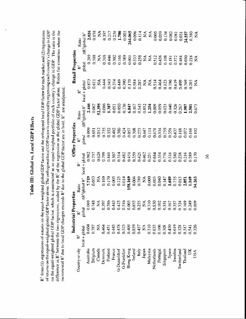
effect, we use econometric methods to separate the two. In Table ifi we report the R2 from

8

regressions in which we separate the GDP factor into local and common components. To do this,

we first regress each GDP series on the equal-weighted global GDP factor and save the residuals.

Next, we use these residuals in a regression, together with the equal-weighted global GDP factor as

variables to explain each real estate market. I.e. in stage 1, we estimate the local GDP factor X1

with the regression: G1, = a+ J67, + ), where G1 is the change in GDP for country i at time

and G is the equal-weighted global GDP factor realization at time t. Tn stage 2, we use X1 and G

as regressors to explain the total return series for a real estate market: 77, =a+flG + 44, + ç and

save the R2 from this regression as RA2. Finally, we use only G as an explanatory

variable: 77, = a+ + and save the R2 from this regression as RB2.

In order to determine the importance of the local GDP component to the global GDP

component, we take the difference in R2 and divide by the R2 from the regression on the global factor

alone. That is: (RA2 -R2)/R2. It is important to note that the number of time-series observations

in each regression is only eleven. Thus, we would expect relatively high R2 from a regression with

two explanatory variables. We have not used adjusted-R2, although this would be appropriate if we

were explicitly testing an hypothesis with this ratio. With these caveats in mind, we use the ratio

on]y for the purposes of indicating the tendency in each market for the local factor to predominate

over the global factor. In fact for most markets, the g]obal factor is most important-- the incremental

variance explained by the local residual variable is less that the amount of variance explained by the

global factor. There are a few markets that differ from this norm, however. We find that Australia,

Canada, Hong Kong, Thailand, U.K. and to some extent, the U.S., Malaysia and Spain are countries

where local GDP effects dominate global influences. We might expect this for the U.S. and the U.K.

9

since the GDP factor is equal-weighted and these two countries' GDP's would obviously have a

larger than equal weight were we using gross GDP weights, or market capitalization weights. This

is not true for some of the other countries, however. The table suggests that, while fundamental

economic factors explain much of the performance of local real estate markets, the effects of local

economic deviations from global trends are more important for some countries, the U.S. included.

111.3 Time-series regressions

Although we have only eleven years of data, it is useful to further consider how the global

GDP factor is r&ated to the fluctuations of property returns. In Table ifi weregress equal-weighted

portfolios of property-types on the equal-weighted GDP factor, and include the one-year lagged

values of GDP changes and the lagged property-type return itself, in order to control for

autocorrelation in the regression error. Note that in each case, the contemporaneous GDP change

is significantly related to returns, and the lagged value is not. In this regard, our time-series results

are broadly consistent with Quan and Titman (1998). This is potentially important, because one

criticism of all appraisal-related real estate data is that itcaptures "asking rents" not "effective rents."

Asking rents are typically sticky and thus area stale measure of real estate markets. The lack of a

lagged relationship between GDP and real estate returns suggests that contemporaneous economic

conditions are reflected in our data. This does not mean our return series' are unpredictable random

walks. lii two of the three regressions, office and retail, the lagged value of the return series is also

significant, indicating strong persistence.

10

1114 US. Time-Series Regression

Although long-term international data is unavailable, we have time-series data for the U.S.

commercial property market that extends from 1960. We use Ibbotson Associates Business Real

Estate total annual return series from 1960 through 1994, and the NCREIF index for years 1995

through 1997. This is the dependent variable in a regression that includes four years of lagged values

and contemporaneous and four lagged values of U.S. GDP growth. The results of this regression are

reported in Table 4. Contemporaneous GDP growth has a coefficient of .65 and is strongly

significant. The inclusion of four lags for each series appears to eliminate the autocorrelation of the

errors in the regression -- the Durbin-Watson statistic is 2. This regression indicates that in at least

one market where we do have long-term data, the relation between GDP growth and real estate

returns is a strong one.

IV. Diversification

The co-movement of real estate markets through exposure to global GDP changes is

potentially meaningful to investors because it suggests that despite the obvious importance of local

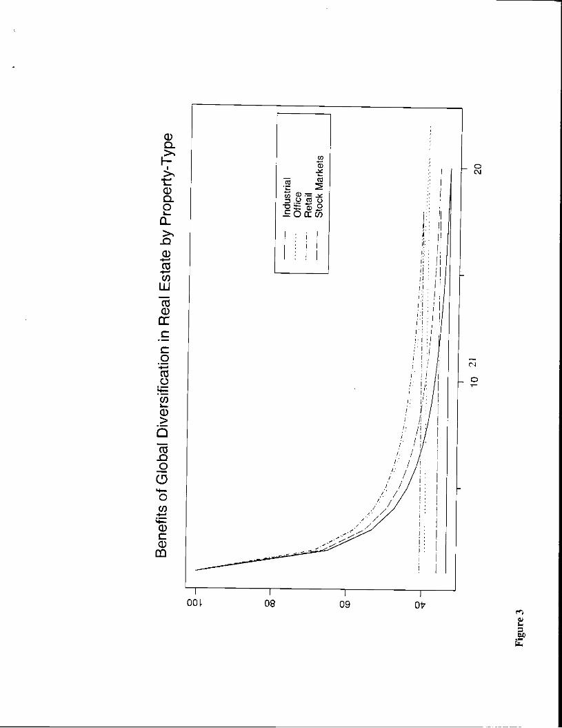
economic conditions to the determinants of property values, diversification has its limits. One way

to explore these limits is to consider how the volatility of a real estate portfolio decreases as more

markets are added to the portfolio. Figure 3 shows the average percentage reduction in volatility

achieved by adding additional countries in sequence, by property type. Country stock markets are

provided for a comparison. The greatest percentage reduction in risk through international

diversification is achieved by the industrial property type and the least percentage of reduction in risk

through international diversification is achieved by office markets. Both office markets and retail

11

markets appear to offer slightly lower relative benefits to international diversification than do equity

markets. In general, however the figure suggests that the international diversification benefits to real

estate are similar in magnitude to those of the equity markets. This is somewhat surprising in light

of the fundamentally location-specific nature of real estate as an investment.

Figure 4 shows the result of removing the global GDP factor from each series. In effect, the

figure shows the results of a portfolio continuously hedged against GDP risk. Notice that the risk

of the industrial portfolio drops considerably, and is well below the equity portfolio limit. The

lower bound is at 13.7 % of the variance of a portfolio with a single country industrial real estate

portfolio investment.

V Conclusions

Our analysis of the re]ationship between changes in GDP and international property returns

suggests that the cross-border correlations of real estate are due in part to common exposure to

fluctuations in the global economy, as measured by an equal-weighted index of international GDP

changes. Country-specific GDP changes help explain more of the variation in real estate returns.

Indeed, in some countries local factors explain considerably more, in percentage terms, than do

global factors. Our study suggests that, while real estate is fundamentally local, demand for space

apparently responds to contemporaneous changes in the global economy. Our analysis of

international diversification suggests that portfolio volatility is reduced by cross-border property

investment, but that only one asset class, Industrial properties, actually yields greater diversification

benefits than international equity market diversification.

12

References

Barry, Christopher-B.. Mauricio Roderiguez and Joseph B.Lipscomb, 1996, "DiversificationPotential from Real Estate Companies in Emerging Capital Markets" Journal of Real EstatePortfolio Management 2(2). 1996, pages 107-18.

Eicholtz, Piet, 1996, "Does International Diversification Work Better for Real Estate than forStocks and Bonds?" Financial Analysts Journal, January-February, 57-62.

Eicholtz, Piet. Ronald Huisman, Kees Koeddijk, Lisa Sehuin, 1998, "Continental Factors inInternational Real Estate Returns" Real Estate Economics 26:3 493-509.

Eicholtz, Piet, 1996, "The Stability of the Covari.ances of International Property Share Returns"Journal of Real Estate Research,11(2), 1996, pages 149-58.

Eichholtz, Piet, Hartzell, David J., 1996"Property Shares, Appraisals and the Stock Market: AnInternational Perspective," Journal of Real Estate Finance and Economics;12(2), March 1996,pages 163-78.

Goetzmann, William and Susan Wachter, 1996, "The Global Real Estate Crash: Evidence FromAn International Database," Yale School of Management Working Paper.

Liu, Crocker and Jian-Ping Mci, 1998, "The Predictability of International Real Estate Markets,Echange Rate Risks and Diversification Consequences," Real Estate Economics 26:1, pp.3-39.

Liu, Crocker, Hartzell, David J.. Hoesli, Martin E., 1997, "Internatitmal Evidence on RealEstate Securities as an Inflation Hedge" Real-Estate-Economics;25(2), Summer 1997, pages193-22 1.

Quan, Daniel C and Sheridan Titman, 1998, "Do Real Estate Prices and Stock Prices Movetogether? An International Analysis," forthcoming, Real Estate Economics.

Renaud, Bertrand, 1994, 'The 1985-1994 Global Real Estate Cycle: Are There LastingBehavioral and Regulatory Lessons?" Journal of Real Estate Literature 5(1), January 1997,pages 13-44.

13

Tab

le I:

Sum

mar

y S

tatis

tics

of R

eal U

.S.

Dol

lar-

Dcn

omin

ated

Ret

urns

S

umm

ary

stat

istic

s fo

r th

e IC

PA

dat

a by

cou

ntry

and

pro

pert

y ty

pe o

ver

the

perio

d 19

87 th

roug

h 19

97. R

etur

ns a

re e

stim

ated

fro

myi

cids

an

d ef

fect

ive

rent

s as

dis

cuss

ed in

the

text

, and

con

vert

ed to

U.S

. dol

lars

and

def

late

d by

the

U.S

. inf

iatio

n ra

te.

Indu

stria

l P

rope

rtie

s O

ffice

Pro

pert

ies

Ret

ail P

rope

rtie

s

Cou

ntry

or c

ity

Geo

met

ric A

rithm

etic

S

tand

ard

Ser

ial

Geo

met

ric

Arit

hmet

ic

Sta

ndar

d S

eria

l G

eom

etric

A

rithm

etic

S

tand

ard

Ser

ial

Ret

urn

Ret

urn

Dev

iatio

n C

orre

latio

n R

etur

n R

etur

n D

evia

tion

Cor

rela

tion

Ret

urn

Ret

urn

Dev

iatio

n C

orre

latio

n

Aus

tral

ia

12.1

0 14

.46

2473

00

7 4.

39

7.56

28

.63

0.39

1.

67

5.77

31

.18

0.57

B

elgi

um

7.51

9.

93

23.8

2 -0

.20

8.34

9.

61

17.1

1 0.

33

11.5

5 14

.13

25.0

5 -0

.50

Can

ada

NA

N

A

NA

N

! •2

.96

4.32

16

.51

0.07

N

A

NA

N

A

NA

D

enm

ark

5.18

6.

73

20.6

0 -0

.16

4.50

5.

14

12.0

7 -0

.25

3.69

4,

76

16.7

8 0.

39

Fin

land

9.

08

13.3

0 30

.53

0.52

4.

54

9.47

32

.98

0.47

10

.24

14.9

5 33

.19

0.25

F

ranc

e 5.

29

7.03

20

.76

-0.0

9 3.

47

5.57

22

.19

0.40

8.

88

11.0

1 22

.70

0.16

G

-Dus

seld

orf

6.58

8.

46

21.2

6 0.

05

7.25

8.

50

17.0

6 0.

18

9.56

11

.42

23.1

0 -0

.20

G-F

rank

furt

2.

96

5,13

20

.40

0.43

7.

61

9.43

21

.29

0.76

7.

37

10.3

9 27

.48

0.41

H

ongK

ong

20.8

6 23

.14

25.2

6 0.

32

16.4

5 22

,79

41.3

4 0.

26

12.6

5 13

.53

14.3

3 0.

05

Irel

and

18.0

1 20

.20

24.1

4 0.

05

11.7

8 13

.25

19.2

9 0.

04

11.5

6 12

.56

15.6

1 0.

70

Italy

11

.18

13.1

6 21

.85

0.24

1.

00

5.16

32

.53

0.46

1.

57

7.06

34

.20

-0.5

4 Ja

pan

NA

N

A

NA

N

? -1

7.35

-1

2.21

31

.33

0.25

N

A

NA

N

A

NA

M

alay

sia

-0.3

3 5,

41

39.9

4 -0

.55

4.19

9.

53

34.2

5 -0

.28

NA

N

A

NA

N

A

Net

herla

nds

10.2

5 11

.61

19.1

9 -0

.04

10.0

8 11

.46

18.7

5 0.

20

7.77

9.

07

17.4

8 -0

.54

Por

tuga

l 28

.99

34.8

8 45

.52

0.43

17

.80

21.0

9 30

.04

0.67

27

.22

31.8

9 42

.18

0.13

S

inga

pore

26

.90

31.0

6 33

.62

-0.5

1 15

.73

18.6

6 27

.68

0.13

12

.61

15.7

5 30

.00

0.66

S

pain

14

.46

21.1

1 44

.60

0.76

3.

81

10.2

8 40

.23

0.51

4.

05

lt.54

46

.12

0.59

S

wed

en

5.88

9.

71

27.2

7 0.

24

2.71

8.

81

35.8

5 0.

22

9.31

15

.10

36.2

7 0.

29

Sw

itzer

land

-5

.18

-3.2

5 22

.72

-0.0

7 -[

0.42

-2

.20

47.4

3 0.

46

-8.5

4 -7

.35

15.8

4 -0

.42

Tha

iland

9.

75

16,8

0 40

.50

-0.1

7 5.

29

12.6

8 45

.94

0.26

27

.20

35.3

1 51

.70

0.36

U

K

13.1

4 15

.82

26.9

2 0.

35

4.12

7.

94

29.8

8 0.

30

4.24

7.

17

24.9

9 0.

18

US

A

7.18

8.

68

18.9

7 0.

49

4.68

4.

95

8.05

-0

.16

NA

N

A

NA

N

A

14

Tab

le 11

: 'I'

est o

f the

Equ

ality

of M

eans

Thi

s ta

ble

repo

rts t

he re

sults

of t

estin

g th

e hy

poth

esis

tha

t the

ave

rage

off-

diag

onal

ele

men

t in t

he c

orre

latio

n m

atrix

of p

rope

rty-

type

ret

urns

acr

oss

coun

trie

s in

the

sam

ple

is e

qual

to

the

aver

age

off-

diag

onal

ele

men

t in

the

cor

rela

tion

mat

rix o

f res

idua

ls t

hat r

esul

t fro

m th

e re

turn

ser

ies

bein

g re

gres

sed

on it

s ow

n ch

ange

in

GD

P. A

ll re

turn

s an

d re

sidu

als

and

GD

P c

hang

es a

re re

al U

.S.

dolla

r den

omin

ated

. P

leas

e no

te,

[-st

atis

tics

have

not

bee

n co

rrec

ted

for

doub

led

off-

diag

onal

val

ues

in t

he c

orre

latio

n m

atric

es.

Indu

stria

l O

ffice

R

etai

l

Ave

rage

Cor

rela

tion o

f Ret

urns

0.

334

0.43

9 0.

363

Ave

rage

Cor

rela

tion

of O

wn

GD

P R

esid

uals

0.

129

0.26

5 0.

162

(-st

at o

f Pai

red

1-te

st o

f dif

fere

nce

11.1

57

11.3

35

10.6

16

Ave

rage

Cor

rela

tion

of W

orld

GD

P R

esid

uals

0.

087

0.27

0 0.

121

(-st

at o

f Pai

red

1-te

st o

f dif

fere

nce

13.4

52

10.8

07

15.7

87

Var

ianc

e R

educ

tion;

Ow

n G

DP

0.

284

0.30

9 0.

199

Var

ianc

e R

educ

tion;

EW

GD

P F

acto

r 0.

7 19

0.

602

0.58

4

15

Tab

le I

II: G

loba

l vs.

Loc

al G

DP

Eff

ects

R2

from

(1)

regr

essi

ons

of re

turn

s on

the

equa

lwei

ghte

d g'

obal

CD

P fa

ctor

and

the o

rtho

gona

l loc

al G

DP

fact

or fo

r eac

h m

arke

t and

(2)

regr

essi

ons

of re

turn

s on

thee

qual

-wei

ghte

d glo

bal G

DPf

acto

ralo

ne. T

heor

thog

onal

loca

l CD

Pfac

tori

s con

stru

cted

by r

egre

ssin

geac

h co

untr

y's

chan

ge in

OD

P on

the

equa

l-w

eigh

ted g

loba

l GD

P fa

ctor

, whi

ch is

con

stru

cted

as

an e

qual

-wei

ghte

d po

rtfo

lio o

f eac

h co

untr

y's

chan

ge in

GD

P.

The

rat

io i

s th

e di

ffer

ence

in R

2 be

twee

n th

e tw

o re

gres

sion

s, sc

aled

by

the

R2

of th

e re

gres

sion

on

the

glob

al G

DP

fact

or a

lone

. R

atio

s fo

r co

untr

ies

whe

re t

he

incr

emen

tal

R2

due

to l

ocal

GD

P ch

ange

s exc

eeds

R2

due

to t

he g

loba

l G

DP

fact

or a

re in

hol

d. 1

(2 a

re u

nadj

uste

d.

Indu

stri

al P

rope

rtie

s O

ffic

e Pr

oper

ties

Ret

ail

Prop

ertie

s C

ount

ry o

r city

R

atio

R

atio

R

atio

lo

cal

+ g

loba

l gl

obal

aR

2/gl

obal

R2

loca

l +

glo

bal

glob

al

AR

2/gl

obal

R2

loca

l +

glo

bal

glob

al

AR

2/gl

obal

R2

Aus

tral

ia

0.60

4 0.

069

7.71

9 0.

962

0.00

9 2.

446

0.87

3 0.

289

2.01

6 B

elgi

um

0.78

7 0.

748

0.05

3 0.

737

0.69

1 0.

067

0.61

1 0.

588

0.03

8 C

anad

a N

A

NA

N

A

0.62

8 0.

012

52.3

95

NA

N

A

NA

D

enm

ark

0.46

4 0.

397

0.16

9 0.

799

0.73

5 0.

086

0.44

4 0.

318

0.39

7 Fi

nlan

d 0.

451

0.38

6 0.

170

0.84

1 0.

352

1.38

7 0.

543

0.44

6 0.

217

Fran

ce

0.4.

45

0.44

3 0.

005

0.50

7 0.

482

0.05

1 0.

374

0.30

2 0.

238

G-D

usse

ldor

f 0.

478

0.42

5 0.

125

0.31

4 0.

300

0.05

0 0.

449

0.16

6 1.

700

0-Fr

ankf

urt

0.52

3 0.

516

0.01

4 0.

482

0.42

4 0.

136

0.39

0 0.

389

0.00

3 Fl

ong

Kon

g 0.

409

0.00

3 15

8.16

9 0.

451

0.05

7 6.

847

0.17

0 0.

001

244.

065

Irel

and

0.85

9 0.

855

0.00

4 0.

359

0.30

8 0.

167

0.58

4 0.

533

0.09

6 Jt

aly

0.45

7 0.

255

0.78

9 0.

425

0.27

5 0.

545

0.28

7 0.

258

0.11

4 Ja

pan

NA

N

A

NA

0.

462

0.44

7 0.

032

NA

N

A

NA

M

alay

sia

0.31

0 0.

310

0.00

0 0.

251

0.11

1 1.

254

NA

N

A

NA

N

ethe

rlan

ds

0.83

3 0.

830

0.00

3 .

0.68

4 0.

678

0.00

9 0.

514

0.51

2 0.

005

Port

ugal

0.

106

0.10

2 0.

040

0.35

4 0.

334

0.05

9 0.

464

0.43

8 0.

059

Sing

apor

e 0.

308

0.33

1 0.

147

0.77

6 0.

759

0.02

3 0.

123

0.10

8 0.

134

Spai

n 0.

450

0.16

7 1.

689

0.51

6 0.

358

0.44

0 0.

196

0.18

1 0.

082

Swed

en

0.61

9 0.

357

0.73

5 0.

580

0.43

7 0.

326

0.61

9 0.

572

0.08

1 Sw

itzer

land

0.

328

0.32

4 0.

013

0.23

8 0.

188

0.26

7 0.

499

0.48

4 0.

031

Tha

iland

0.

517

0.16

9 2.

051

0.21

6 0.

072

1.98

7 0.

769

0.03

0 24

,557

U

K

0.54

1 0.

249

1.16

9 0.

589

0.16

8 2.

501

0.28

5 0.

218

0.38

0 U

SA

0.32

6 0.

009

34.2

63

0.17

0 0.

102

0.67

3 N

A

NA

N

A

16

Tab

le I

V:

Tim

e-Se

ries

Reg

ress

ion

of P

rope

rty-

Typ

e Po

rtfo

lios

on A

GU

P Fa

ctor

Res

ults

from

reg

ress

ions

of e

qual

-wei

ghte

d pro

pert

y-ty

pe p

ortf

olio

s on

an

equa

l-w

eigh

ted G

DP

fact

or

over

the

peri

od 1

987

thro

ugh

1997

. Indu

stri

al

Off

ice

Ret

ail

coef

[-

stat

co

ef

I-st

at

coef

t-

stat

Inte

rcep

t 0.

010

0.22

7 0.

005

0.12

3 -0

.013

-0

.329

Equ

al-W

eigh

ted G

DP

1.

321

3.56

0 0.

808

1.87

6 1.

160

3.22

4

Equ

al-W

eigh

ted

GD

[-1]

-0

.369

-0

.588

-.

86!

-1.3

44

-0.3

43

-0.6

47

Pro

pert

y Po

rtfo

lio [-

I]

0.48

0 0.

350

0.70

9 2.

325

0.58

7 2.

307

Dur

bin-

Wat

son

1.86

1.

78

1.48

R-S

quar

e 0.

76

754

.778

17

Tab

le V

: U

.S. B

usin

ess

Rea

l Est

ate

tota

l Ret

urn

and

Cha

nges

in U

.S. G

DP

U.S

. Bus

ines

s Rea

l Est

ate

is ta

ken

fror

nlbb

otso

n A

ssoc

iate

s E

nCor

rda(

abas

e and

mea

sure

s th

e to

tal r

etur

n to

a p

ortfo

lio of

com

mer

cial

real

est

ate

over

the

perio

d 19

60 th

roug

h 19

94.

For

199

5 th

roug

h 19

97, t

he N

CR

EIF

tot

al re

turn

inde

x is

use

d.

Per

iod:

196

0- 1

997

Coe

ffic

ient

T

-Sta

tistic

Inte

rcep

t -0

.044

-1

.450

GN

P

0.53

3 2.

178

GN

P t-

1 -0

.399

-1

.436

GN

P t-

2 0.

779

2.74

2

GN

P t-

3 -0

.2 17

-0

.691

GN

P t-

4 0.

407

1.35

0

Bus

ines

s Rea

l E

stat

e t-

1 1.

068

5.20

8

Bus

ines

s R

eal

Est

ate

t-2

-0.7

16

-2.4

83

Bus

ines

s R

eal

Est

ate

t-3

0.33

1 1.

164

Bus

ines

s R

eal

Est

ate

t-4

-0.2

24

-1.1

61

Dur

bin-

Wat

sop

2.03

R-s

quar

ed

0.78

5

18

I .20

1.00

0.80

0.60

0.40

0.20

0.00

-0.2

0

-0.4

0

-0.6

2

Tim

e • Au

stra

lia!

Bel

gium

I • De

nmar

k I

• Finl

and

I F

ranc

e I

• 6-D

usse

ldor

f I • G-

Fra

nktu

rt I

l-Ion

gKon

g I

• Irela

nd I

Italy

M

alay

sia

I N

ethe

rland

s I

Por

tuga

l I

F

Sin

gapo

re I

Till

Spa

in I

Sw

eden

I T

i Sw

itzer

land

T

haila

nd I

UnK

ingd

om I

US

A I

Aus

tral

ia 0

Bel

gium

0

Can

ada

0 D

enm

ark

0 • Fi

nlan

d 0

Fra

nce 0

G-D

usse

ldor

t 0

G-F

rank

furt

0

Hon

gKon

g 0

Irel

and

0 • Ita

ly 0

Ja

pan

0 • M

alay

sia 0

Net

herla

nds 0

P

ortu

gal 0

S

inga

pore

0

Spa

in 0

Sw

eden

0

iiTi S

witz

erla

nd 0

T

haila

nd 0

T

i UnK

ingd

om 0

U

SA

0

Aus

tral

ia R

B

elgi

um R

D

enm

ark

R

Fin

land

R

• Fra

nce

R

G-D

usse

ldor

l H

• G-F

rank

lurt

H

. I-

iong

Kon

g R

Irel

and

H

Italy

A

Net

herla

nds A

P

ortu

gal H

fl S

inga

pore

R

Spa

in R

• Sw

eden

H

• Switz

erla

nd H

• Th

aila

nd H

U

nkin

gdon

i A

Fig

ure

1 A

nnua

l R

etur

ns F

or a

ll M

arke

ts a

nd P

rope

rty T

ypes

: 19

87 -

199

7

19

Ret

urn

Val

ues

1.48

I .40

Dec

D

ec

1987

1988

Dec

1989

1Q90

1901

1992

1993

1994

Dec

Dec

1995

1996

Dec

1997

Ret

urn

Val

ues

0.34

—

0.28

—

0.24 —

-0,04—-'

-0.08—

-0.12—

-0.16——

-0.2

0

-0,2

4—

-0.2

8—

-0.3

2—

I II

Tim

e

biLi

1t

• Fran

ce G

• G

erm

any

G • Ho

ngK

ong

C

Irel

and

C

Ti S

inga

pore

I

Spa

in G

T

i Sw

eden

C

Sw

itzer

land

C

0.20

—

0.16

—

0.12

—

0.08

—

0.04

—

0.00

—

Li II

II .1

1

-0.3

6 I Dec

I Dec

D

ec

I Dec

D

ec

Dec

D

ec

Dec

I Dec

F

Dec

1967

1988

1989

1990

1991

1992

1993

• Aust

ralia

C

Fl B

elgi

um C

• C

anad

a C

• D

enm

ark

G

' F

inla

nd C

• Ital

y C

0 T

haila

nd C

Ja

pan

C

UnK

ingd

om C

M

alay

sia

C

US

A C

• Ne

ther

land

s C

T

i Por

tuga

l C

Figu

re 2:

Dol

lar-

Den

omin

ated

chan

ges

in G

DP

defl

ated

by

the

u.g9

cpi,

1987

-. 19

97

Dec

1997

Ben

efits

of G

loba

l D

iver

sific

atio

n in

Rea

l Est

ate

by P

rope

rty-

Typ

e 0

-___

____

____

____

____

__

0-

0 I __

Indu

stria

l I

Offi

ce

I R

etai

l

L S

tock

Mar

kets

0 (0 -

10

2!

20

Fig

ure

3

Ben

efits

of G

DP

-Hed

ged

Glo

bal D

iver

sific

atio

n in

Rea

l E

stat

e by

Pro

pert

y-T

ype

0 0-

0

"N'

\\'N

\\' N'. N

N

. -.

— _

±

.±

0 __

____

____

____

____

_ (0

0 0 c,'J

10

20

Fig

ure

4

22

Indu

stria

l O

ffice

I

Ret

ail

L S

tock

s