y0i7n.applied.finite.element.modeling
DESCRIPTION
dTRANSCRIPT
about the book . . .
Bridging the gap between theoretical texts and program user’s manuals, this hands-on training tool helps engineers solve problems by formulating a cost-effective model con- sistent with proper finite element usage.
Providing far more guidance than any other book in its field, Applied Finite Efement Modeling takes the engineer step by step through the stages of problem definition, modeling, and solution presents six simple, practical example problems. as well as nine industry-standard benchmark problems, to illustrate modeling steps, demonstrate results, and show the effects of various element types and densities on accuracy covers dynamic and thermal analysis, substmcttig,,and linear statics and discusses how to calibrate the accuracy of timte element analyses.
With guidelines in generic finite element terminology-independent of any one com- mercial finite element program-this reference is essential reading for all users of finite element analysis techniques. including mechanical, srmctural, and civil design engineers; structural. vibrations, and stress analysts; and advanced undergraduates and graduates in the above disciplines.
about the author . .
JEFFRF( M. S~VLE is a supervisor of a Mechanical Engineering Group at Eastman Kodak Company in Rochester, New York. Prior to that he served as Manager of Engineering for Suess Technology Inc. in Rochester. He has published numerous articles in leading engineering magazines, including a 34-part series entitled “A Manager’s Guide to Finite Element Analysis” that appeared in Computer Aided Engineering Magazine from 19&1- 1987. Mr. Steele has lectured widely on finite element modeling, led workshops, taught college seminars, and contributed papers to conferences throughout the U.S. He is a member of the American Society of Mechanical Engineers. He received the B.S. degree (1973) in mechanical engineering from Lehigh University in Bethlehem, Pennsylvania, and M.S. degree (1978) in mechanical engineermg from the Rochester Institute of Technology.
Printed in the Unitei Slates OfAmuica ISBN: O-8247-8048-5
marcel dekker, Inc./new york . basel. hong kong
AWLleD FINITE
GUMNT MODELING
PRACTICAL PROBLEM SOLVING fOR ENGINEERS
Applied Finite Element
Modeling Practical Problem Solving for Engineers
JEFFREY M. STEELE Eastman Kodak Company
Rochester, New York
Marcel Dekker, inc. New York and Base1

Library of Congress Cataloging-in-Publication Data
Steele, Jeffrey M., [date] Applied finite element modeling.
(Mechanical Engineering ; 66) Includes index. 1. Finite element method. 2. Engineering--Mathematical
models. I. Title. II. Series : Mechanical engineering (Marcel Dekker, Inc.) ; 66. TA347.F5S74 1989 620’.001’515353 88- 36332 ISBN O-8247-8048-5 (alk. paper)
This book is printed on acid-free paper.
Copyright 0 1989 by MARCEL DEKKER, INC. All Rights Reserved
Neither this book nor any part may be reproduced or transmitted in any form or by any means, electronic or mechanical, including photocopying, microfilming, and recording, or by any information storage and retrieval system, without permission in writing from the publisher.
MARCEL DEKKER, INC. 270 Madison Avenue, New York, New York 10016
Current printing (last digit) : 10 9 8 7 6 5 4 3 2
PREFACE
This book is intended to fill a gap in the information available to users of the finite-element method. The vast majority of finite element analyses is performed with commercial finite-element pro- grams that provide documentation on coding input data and the mathematical basis for that particular program. In addition, there are a number of excellent textbooks on the theory and mathemati- cal fundamentals of the finite element method. This book is in- tended to bridge the gap between the theoretical texts and the program user’s manuals.
Practicing engineers, when faced with a real engineering prob- lem to solve, need to answer questions such as “Is this problem applicable to finite element analysis ?‘I “What type of model should be used?” “What type of elements and how many?” and “How ac- curate will the results be. 7” Extracting specific information from the theoretical texts to answer questions like these is difficult, especially for the novice.
PRINTED IN THE UNITED STATES OF AMERICA
i i i

iv / Preface v / Preface
As little as 10 years ago, finite element analysis was performed by specialists, trained at a graduate level, using mainframe com- puters. The rapid decrease in computing cost and the availabil- ity of engineering workstations and personal computers have brought along a new group of users who are not full-time ana- lysts but use finite element analysis as another tool in their de- sign and analysis work. These users may or may not have the benefit of formal training in the finite element method. It is for these users that this book is primarily intended. This book is not intended as a substitute for formal training, and a full col- lege-level course is recommended for anyone seriously using the finite element met hod. This book provides guidance to the finite element user in building a cost-effective model and in thinking through the entire modeling process before sitting down at a computer terminal.
Although the price of mainframe hardware is decreasing, there is still a need for reasonable, cost -effective models. Good results cannot be achieved by simple overkill. In addition, most hard- ware still has limitations, especially workstations and personal computers.
Chapter 2 provides an overview of the mathematical fundamen- tals of the finite element method and gives references to a few texts recommended for more complete information. Topics for inclusion in this chapter were selected to be consistent with the material covered in the following chapters. Although topics such as substructuring and dynamics may be considered advanced by some standards, they are in common use and are therefore in- eluded .
Chapters 3, 4, 5, and 6 cover the basics of modeling. Chap- ter 3 on required input data is for the first-time user. Chapters 4 and 5 walk the reader through model development as a three- step process : (1) problem definition, ( 2) free-body diagram, and (3) finite element model. A set of simple components is in- cluded in Chapter 4 and carried through the subsequent chapters as example problems.
Chapters 7 and 8 discuss performance of the various element types, including the effects of element distortion. Most of the problems in these chapters were provided by a paper proposing a set of finite element benchmark problems by R . H. MacNeal and R. L. Harder of the MacNeal Schwendler Corporation. Data in these chapters were generated with MSC/NASTRAN and ANSYS . The elements are described as generically as possible without referencing the program or version.
Chapters 9 through 12 deal with more advanced topics such as refined mesh modeling for stress concentration effects, sub- structuring, dynamics, and thermal analysis.
Chapter 13 provides some ideas for assessing the accuracy of finite element analyses. Rather than be a set of rigid guidelines, this chapter is intended as food for thought and will, I hope, stir some interest in a topic that has not received as much attention as deserved.
I would like to express my appreciation to Dr. Neville F. Rieger, my colleague and former employer, for suggesting the topic for the book over 12 years ago. Also, I would like to thank the MacNeal Schwendler Corporation for the use of their set of benchmark problems and data that forms the basis for much of Chapters 7 and 8; the people of Swanson Analysis Systems, Inc., with whom I have enjoyed a good working relationship over the past eight years; and the editors of Computer Aided Engineering for pub- lishing “A Manager’s Guide to Finite Element Analysis.” This series of articles served as a testing ground for many of the ideas that later found their way into this book. And finally, I express my gratitude to my wife Julie for her patience and sup- port through all the hours of computer runs and typing.
Jeffrey M. Steele

CONTENTS
Preface
1. Introduction to the Finite Element Method
2. Fundamentals of the Finite Element Method
2.1 2.2 2.3 2.4 2.5 2.6 2.7 2.8 2.9
Terminology Element Discretization Isoparametric Concept Isoparametric Shape Functions Stress, Strain, and Stiffness Formulations Element Equation Assembly and Solution Element Types Element Integration Order Dynamic Analysis
. . . III
5
5 6 8
11 13 15 21 27 31
vii

viii 1 Contents Contents / ix
2.10 Substructuring 32 2.11 Generalized Field Problems 37 2.12 Summary 38
7. Element Performance 141
7.1 Element Integration Order 146 7. 2 Element Performance Tests 149 7.3 Simple Beam in Bending 151 7.4 Curved-Beam Benchmark Case 157 7.5 Twisted-Beam Benchmark Case 163 7.6 Rectangular Plate Benchmark Case 168 7.7 Scordelis-Lo Roof Benchmark Case 175 7.8 Spherical Shell Benchmark Case 177 7. 9 Thick-Walled Cylinder 180 7.10 Rotating Disk Benchmark Case 182 7.11 Summary 187
3. Basic Input Data 41
3.1 Geometry Definition 42 3.2 Material Properties 43 3.3 Displacement Constraints 47 3.4 Applied Forces 47 3.5 Automatic Mesh Generation 52 3.6 Data Input Format 53 3.7 Summary 54
8. Element Distortion 189 4. Problem Definition 55
8.1 Simple Beam : One Layer of Elements 192 8.2 Effect of Numerical Integration Order 194 8.3 Simple Beam : Three-Element Layers 198 8.4 Summary 203
4.1 Problem Definition 56 4.2 Example Cases 59 4.3 Free-Body Diagram 72 4.4 Free-Body Diagram : Example Cases 78 4.5 Summary 80
207 9. Refined Mesh Modeling
9.1 Refined Modeling Concept 208 9.2 Right-Angle Beam Example Case 211 9.3 Refined Modeling: Example Cases 226 9.4 Plate-Solid Transitions 247 9. 5 Thermal Effects 253 9.6 Summary 253
5. Finite Element Model 81
5.1 Element Density 82 5.2 Element Distortion 86 5. 3 Boundary Conditions 86 5.4 Finite Element Model: Example Cases 87 5.5 Summary 125
10. Substructuring 255 6. Debugging Finite Element Models 131
10.1 Substructuring Procedures 255 10.2 Practical Considerations 257 10.3 Example: Circular Plate 259 10.4 Example: Gear Segment 263 10.5 Turbine Blade Attachment: Refined Model 270 10.6 Summary 273
6.1 Geometry 132 6.2 Material Properties 137 6.3 Applied Forces 137 6. 4 Displacement Constraints 138 6.5 Summary 138
x / Contents
11. Dynamic Finite Element Modeling 277
11.1 11.2 11.3
11.4
11.5 11.6 11.7 11.8 11.9
Overview of Dynamic Modeling Considerations Mathematical Fundamentals Dynamic Finite Element Modeling Considerations Modeling Considerations for the Three Types of Analysis Transient-Response Analysis Forced Harmonic-Response Analysis Damping Dynamic Substructuring Summary
12. Thermal Analysis with Finite Element Analysis 327
12.1 Primer on Heat Transfer 328 12.2 Thermal Finite Element Analysis 330 12.3 Thermal Modeling Consideration 331 12.4 Example : Pressure Vessel 333 12.5 Summary 339
13. Calibrating the Accuracy of Finite Element Models
13.1 Sources of Uncertainty 13.2 Methods of Calibration 13.3 Summary
Index 35s
277 278
283
285 311 312 316 318 320
341
342 350 358
Applied Finite Element
Modeling
1
INTRODUCTION TO THE FINITE ELEMENT METHOD
The finite element method of engineering analysis is relatively new and can trace its roots back to the mid-1950s. The paper that signaled the beginning of finite element analysis was written in 1956 by Turner et al. [ 11. The finite element method requires the use of modern digital computing equipment with floating-point capability and considerable memory and disk capacity. For this reason, the development and popularity of the method has closely followed the evolution of computing hardware over the past 30 years.
The finite element method has been applied to a wide variety of engineering problems in which complex geometry has not al- lowed the use of a simple closed-form solution. The method’s versatility and popularity stem from the use of simple shapes, known as elements, to be assembled together to model geometri- cally complex structures.
The first major finite element code for general use was NAS- TRAN developed for NASA by the MacNeal-Schwendler Corpora- tion and Computer Sciences Corporation in the mid- 1960s. As

2 I Chapter 1
with the early work of Turner et al., it had its roots in the aero- space industry. The method was applied to other areas of struc- tural analysis in mechanical and civil engineering. The ANSYS code had its roots in the nuclear industry and was introduced in 1970 by Swanson Analysis Systems Inc. Zienkiewicz published his text [ 21 in 1971 with emphasis on civil as well as mechanical engineering applications.
A significant step in finite element development occurred in 1968 with the paper by Irons and Zienkiewicz that advanced the isoparametric element concept [ 31 . Another significant contribu- tion was the introduction of the frontal solution algorithm by Irons in 1970 141. The frontal solution routine made the finite element method more adaptable to a wider variety of hardware.
The finite element method has been expanded to nonstructural field problems such as heat transfer, fluid flow, and magnetics. In 1965, Zienkiewicz and Cheung’s findings appeared [ 51 and in 1966, Wilson and Nickell’s [ 61.
In the late 1960s and into the 197Os, the application of the fi- nite element method required the use of a large mainframe com- puter . Most applications were run on IBM and Control Data ma- chines that had memory and precision sufficient to handle the large sets of matrix equations generated during a calculation. The majority of the analyses were performed by specialists with training in applied mechanics, finite element methods, use of com- puter software, and use of the finite element code. Input data had to be carefully coded because there was a significant cost per second on the computer and errors in data input, or data entry could result in significant wasted costs.
In the late 1970s) the introduction of super-minicomputers such as the Digital VAX, the Prime, and the Data General Eclipse made it possible to bring the necessary hardware into the engi- neering department. With these machines, it was possible for design and analysis engineers to use finite element analysis as part of their work without necessarily relying on the support of a finite element specialist. The development of engineering work- stations in the early and mid-1980s such as the Apollo, the Sun, and the Microvax helped to further promote the use of finite ele- ment applications. With the cost per second of computing use de- creasing at a rapid rate, the cost of finite-element analysis de- creased to a point where engineers were not restricted by com- puter costs. The development of the Intel 80286/80287-based PC/AT in the mid-1980s and its clones made possible the porting of some finite element codes onto a desktop machine. Although the PC machines have fixed memory and do not have their own
Introduction to the Finite Element Method / 3
virtual memory capability, they are still capable of running modest finite element problems. It is only a matter of time until the engl- neer will have a desktop machine, with a full 32-bit capability and virtual memory at his disposal. This entire hardware evolution has made it possible for the average engineer to have the capabil- ity to use finite element analysis as another design and analysis tool.
The objective of this book is to bridge the gap between the ex- cellent texts that have been written on the finite element method [2, 7-101 and the user’s data input instructions for the various finite element codes. The intention of this book is to give the novice or part-time finite element user information on the model- ing process in general. Information is presented in a generic sense without tying it directly to one or another specific finite- element code. A genera1 overview of the basis for the finite ele- ment method is given in Chapter 2; however, it is not intended as a substitute for the more comprehensive texts given above.
Subsequent chapters give guidelines and recommendations for going from an engineering problem to a finite element calculation including defining the problem, developing the most cost-effec- tive model, and interpreting the results. Although there are many finite element codes available, each with a different data input scheme, there is a common set of basic input data required for each. The objective of an engineer using finite element anal- ysis is to work from the engineering problem to develop a model that will give him suitable accuracy at a reasonable price in terms of analysis and computer time.
REFERENCES
Turner, M. J., R. W. Clough, H. C. Martin, and L. J. Topp, “Stiffness and Deflection Analysis of Complex Structures ,I1 Journal of Aeronautical Science, Vol. 23, 1956, pp. 805- 824. Zienkiewicz, 0. C. , The Finite Element Method in Engineer- ing Science, 2nd ed. , McGraw Hill, London, 1971. Irons, B. M. and 0. C . Zienkiewicz, “The Isoparametric Fi- nite Element System - A New Concept’in Finite Element Anal- ysis , I’ Proceedings of the Conference on Recent Advances in Stress Analysis, Royal Aeronautics Society, 1968. Irons, B. M., “A Frontal Solution Program for Finite Element Analysis, ‘I International Journal for Numerical Methods in En- gineering, Vol. 2, No. 1, Jan. 1970, pp. 5-23.

4 I Chapter 1
5.
6.
7.
8.
9.
10.
Zienkiewicz, 0 .C. and Y. K. Cheung, “Finite Elements in the Solution of Field Problems,” The Engineer, Sept. 1965, pp. 507-10. Wilson, E. L. and R. E. Nickell, “Application of the Finite Element Method to Heat Conduction Analysis,” Nuclear En- gineering and Design, Vol. 4, 1966, pp. 276-286.
Cook, R. D., Concepts and Applications of Finite Element Analysis, Wiley, New York, 1974.
Gallagher, R. H., Finite Element Analysis Fundamentals, Prentice Hall, Englewood Cliffs, N. J. , 1975. Heubner, K. H., The Finite Element Method for Engineers, Wiley, New York, 1975. Bathe, K. J. and E. L. Wilson, Numerical Methods in Finite Element Analysis, Prentice-Hall, Englewood Cliffs, N. J. , 1976.
2
FUNDAMENTALS OF THE FINITE ELEMENT METHOD
The mathematics of the finite element method can be complex. This chapter gives a broad overview of the fundamentals of the method, but does not attempt to give a rigorous treatment of the mathematics, There are many excellent texts on the fundamen- tals of the finite element method and the reader is referred to them as sources of basic information. They include [ 1, 3, 4, 7-91.
2.1 TERMINOLOGY
The finite element method operates on the assumption that any continuous function over a global domain can be approximated by a series of functions operating over a finite number of small sub- domains. These series of functions are piecewise continuous and should approach the exact solution as the number of subdomains approaches infinity.

6 I Chapter 2 Fundamentals of the Finite Element Method I 7
1. The global domain is divided into subdomains called elements. 2. The points defining and connecting the elements are called
nodes or nodal points. 3. The function that exists over the domain is explicitly solved
for at the nodal points, i.e. , nodal variables. It is assumed that the value of the function at any point internal to an ele- ment can be defined in terms of that element’s nodal vari- ables. The nodal variables are referred to as degrees of freedom. This term applies specifically to stress analysis in which the nodal variables are the deflections of the struc- ture at the nodal points; however, the term is often used generically to refer to all nodal variables.
Although the elements are specified as joined at their common nodes, they are assumed to be continuously coupled along their common boundary and any function is assumed to be continuous at the boundaries, although continuity of slope is not necessarily maintained. The complete collection of elements represents an ap- proximation of the domain’s geometry as a continuum. The nodal points are only reference points for evaluation of the function and do not represent physical points of connection within the domain.
2.2 ELEMENT DISCRETIZATION
The concept of element discretization can be illustrated by a finite element model of a tapered beam in tension as shown in Figure 2.1. The domain is the two-dimensional plane of the beam. The function to be evaluated is the displacement field in the axial direction. There is a force in that direction, and one degree of freedom per node. The beam is divided into three elements and four nodes. A force is applied to node 4, and node 1 is constrained against having any displacement.
The stiffness functions for each of the three elements can be formed by the relationship
k = EAIL (2.1)
where
k = stiffness lbflin. 2 E = Young’s modulus A = the average cross-sectional area of the element L = the length of the element
The three element stiffnesses may be calculated, assuming unit thickness and E = 30,000,OOO psi, as
* w 3.00
Fl kl F2 k2
F3 k3
Resulting Equivalent Spring Model
Figure 2.1 Finite-element model of a tapered beam: Beam in ten- sion divided into three one-dimensional elements.
Element 1 Aave = 0.167 in.2 kl = 5,000,OOO lbf/in.
Element 2 Aave = 0.500 in. 2 k, = 15,000,OOO lbf/in.
Element 3 Aave = 0.833 in. 2 k, = 25,000,OOO lbf/in.
The nodal variables to be solved for, i.e. , the degrees of free- dom, are the axial displacements of each of the nodes di. Assem- bling a set of equations to represent the beam gives
Equation 1 k,(d, - d2) = F, - F, (2.2)
Equation 2 kz(d, - d3) = F2 - F3
Equation 3 k,(d, - d,) = F, - FI,
where
dt = axial displacement of node i Fi = axial force at node i
8 / Chapter 2
Writing these equations in matrix form for element 1 gives
(2.3)
The matrix set of stiffness equations for the other elements is of the same form.
The assembled set of matrix equations describing the entire beam is
I
k, -kl -kl k,+k, -k,
-k2 k, + k, -k,
-k, k3
dl d, I(1 = d3 d, Fl FZ (2.4)
F3 F4 This set of matrix equations represents four equations in four un- knowns, di, which can be solved to characterize the response of the beam to an axial applied force.
Although this example illustrates the principle of assembling element stiffness equations into a global set of equations, actual formulation of the individual element stiffness matrices for two- dimensional and three-dimensional solid elements is significantly more complex. Some advanced three-dimensional solid elements have 20 nodes and 60 degrees of freedom per element represented by a 60 x 60 set of equations for each element.
2.3 ISOPARAMETRIC CONCEPT
In order to develop stiffness equations for two-dimensional and three-dimensional solid elements, there need to be interpolation functions that will give the value of a variable at an interior point of the element as a function of the nodal values. These interpola- tion functions are typically referred to as shape functions. For an element in an x, y coordinate system, the displacement at some element interior point may be specified as
4 d(x, y> = c Ni(x> Y) di
i=l (2.5)
Fundamentals of the Finite Element Method / 9
where
d( x , y) = displacement at global coordinates x , y di = nodal displacement values Ni(x, y) = shape functions for each node and a function of x
and y
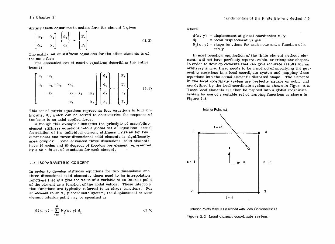
In most practical application of the finite element method, ele- ments will not have perfectly square, cubic, or triangular shapes. In order to develop elements that can give accurate results for an arbitrary shape, there needs to be a method of specifying the gov- erning equations in a local coordinate system and mapping these equations into the actual element’s‘distorted shape. The elements in the local coordinate system are perfectly square or cubic and are defined by the local coordinate system as shown in Figure 2.2. These local elements can then be mapped into a global coordinate system by use of a suitable set of mapping functions as shown in Figure 2.3.
Interior Point s,t
t=-1
Interior Points May Be Described with Local Coordinates: s,t
Figure 2.2 Local element coordinate system.

10 / Chapter 2 Fundamentals of the Finite Element Method I 11
ELEMENT IN GLOBAL COORDINATE SYSTEM
Functions Described over a Local, Square Area May Be Mapped into the Global Element Shape
ELEMENT IN LOCAL COORDINATE SYSTEM
In this manner, both two- and three-dimensional elements can be mapped into any reasonable quadrilateral or prism shape. More important, when the elements have midside nodes in addition to their corner nodes, the elements can match a curved boundary in the global system. The global coordinates for any point in the element can be specified in terms of that point’s local coordinates and the global coordinates of the nodes
n x(s, t) = c Ni’(s, t) xi
i=l
where
x(s, t> = global coordinate of point s, t n = the number of nodes Ni’(s, t) = mapping function for node i xi = x coordinate for node i
In the same manner, the y coordinate is
y(s, t) = 5 N.‘(s, t) Y i=l ’ i
(2.6)
(2.7)
The definition of an isoparametric element is one that uses the same functions to map the coordinates as it uses to interpolate nodal va- riables, i.e. ,
N’(s, t) = N(s, t) (2.8)
The isoparametric concept is thoroughly discussed by Zienkiewicz in [l].
2.4 ISOPARAMETRIC SHAPE FUNCTIONS
For a two-dimensional quadrilateral with corner nodes as shown in Figure 2.4, the isoparametric shape functions can be given by
N1 = l/4(1-s)(l-t)
N, = 1/4(l+s)(l-t)
N3 = 1/4(l+s)(l+t) (2.9)
Figure 2.3 Local to global element mapping. N, = l/4(1-s)(l+t)

12 I Chapter 2
A Function May Be Evaluated at an Interior Point of an Element by Summing the Value of the Function at the Nodal Points, Multiplied by the Appropriate Weighting Factors
2
Interior Point s,t
$(s,t) = Ni#
\
Figure 2. 4 Quadrilateral element.
Several items should be noted regarding these shape functions.
They are linear polynomial functions. Both the coordinates and nodal variables are linearly interpolated within the ele- ment . This can be better illustrated by considering interpo- lation in the local s direction along the “top” surface of the element (Figure 2.5)) i.e., t = 1 between nodes 3 and 4 where the shape functions become
N, = 1/2(l+s)
N,, = 1/2(1-s) (2.10)
The shape function for a given node i has a value of 1.0 at node i and a value of 0.0 at each of the other nodes.
At any given local point (s, t), the sum of all four shape func- tions must equal 1.0.
3
Fundamentals of the Finite Element Method I 13
Q = N343 + N4+4
= 0.5(1+s) +0.5(1-s)
S
--It- 4 rs t= 1.0 S
For One Dimension the Value of the Function at the Interior Point Is the Weighted Average of the Two Corner Node Values The Weighting FunctionsAre Linear and Based on the Distance from the Interior Point to the Node
Figure 2.5 One-dimensional linear interpolation.
2.5 STRESS, STRAIN, AND STIFFNESS FORMULATIONS
Given the two-dimensional element shown in Figure 2.4, the strain at any point in the element can be given by the strain vector
(2.11)
where
EX = strain in the x direction = duldx
EY = strain in the y direction = dvldy
ExY = shear strain in the x-y plane = duldy + dvldx
The shape functions are used to obtain these derivatives with respect to the nodal displacements. For example,
n E x = du/dx = dldx c Niui [ 1 i=l
(2.12)

14 I Chapter 2 Fundamentals of the Finite Element Method / 15
The y direction strain and shear strain can be obtained in a simi- lar manner.
The complete calculation of strain can be given in matrix form
The element stiffness matrix for a two-dimensional element is generated by integrating the product of the transpose of the B matrix, the D matrix, and the B matrix over the element area (or volume in the case of three-dimensional solid elements), i.e. , as
{El =
dNi/dx.. .dN,/dx 00.. .OOO
ooo...oo dNi/dy.. .dN,/dy
dN,/dy.. .dN,/dy dN,/dx.. .dN,/dx
1
Ul . . .
un
Vl . .
vn
The matrix of shape function global derivatives is known as the [B] matrix and is also referred to as the strain-displacement ma- trix. The above set of equations can be given in matrix form as
IE} = tB1 Id] (2.13)
Stress and strain can be related by the use of an elasticity matrix [Dl.
(01 = WI (~1 (2.14)
For two-dimensional plane stress and isotropic materials, the elas- ticity matrix is
-I
(2.15)
For two-dimensional plane strain and isotropic materials, the elas- ticity matrix is
[
1 P/cl-u) 0
[Dl = E(I-u) 1.1/(1-lJ) 1 0 1 (2.16) (l+l-4)(1-2u) o 0 (I-2lJ)/2(1-u)
In order to convert nodal displacements into stresses, the B and D matrices are combined.
(01 = [Dl [Bl Cd] (2.17)
It should be noted that the above relationships hold at one specific point within the element as defined by the local coordinates used in the shape functions Ni whose derivatives are in [B].
[kl = /[BITID LB1 dx dy (2.18)
where [k] is the element stiffness matrix and the relationship be- tween stiffness, applied forces, and nodal displacements is given by
[kl id] = {F] (2.19)
2.6 ELEMENT EQUATION ASSEMBLY AND SOLUTION
There are two methods commonly used to assemble and solve the element matrix sets of equations: the banded equation solver and the wavefront equation solver.
In the banded solver method, the entire global set of equa- tions from all elements is first assembled and then reduced. The method of assembling the individual element stiffness matrices in- to a global stiffness matrix follows the same form as shown in the simple example in Section 2.2 and in Equation 2.4.
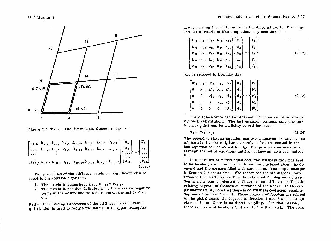
The element force and displacement vectors, and stiffness co- efficients are set up according to the order of the global degrees of freedom. For example, if a particular element is bounded by nodes 1, 2, 10, 9 (degrees of freedom 1, 2, 3, 4, 19, 29, 17, 18) as shown in Figure 2.6, then the element stiffness coefficient in row 1 and column 7 represents the relationship between a force at local degree of freedom 1 (1st node, x direction) and a dis- placement at local degree of freedom ‘7 (4th node, x direction).
'%,I kl,z'Q,, k,,,'%,s kl,6k1,7k1,6
k2,, k2.1, k,,, k,,, k2.7 b,,
In the global system, this relates node 1, x direction and node 9, x direction (degree of freedom 1’7) so that the coefficient would be assembled into the global matrix at row 1, column 17.
16 I Chapter 2 Fundamentals of the Finite Element Method I 17
dl
Figure 2.6 Typical two-dimensional element gridwork.
kl,, kl,, kl.3 kl,, kl,lg k 1,20
k 291 k2,2 b,3 k2,4 k2 ,lg k2,2o . . .
. . .
kle.1 kle.2 klo,3 klo.4 klo,lg k 18.20
(2.21)
Two properties of the stiffness matrix are significant with re- spect to the solution algorithm.
1. The matrix is symmetric, i.e. , k, ,i7 = k,,,i. 2. The matrix is positive-definite, i.e., there are no negative
terms in the matrix and no zero terms on the matrix diag- onal.
Rather than finding an inverse of the stiffness matrix, trian- gularization is used to reduce the matrix to an upper triangular
form, meaning that all terms below the diagonal are 0. The orig- inal set of matrix stiffness equations may look like this
and is reduced to look like this
(2.22)
(2.23)
The displacements can be obtained from this set of equations by back-substitution. The last equation contains only one un- known d s that can be explicitly solved for, i.e. ,
d, = F’5/k’5,5 (2.24) The second to the last equation has two unknowns. However, one of those is d,. Once d, has been solved for, the second to the last equation can be solved for d,. The process continues back through the set of equations until all unknowns have been solved for.
In a large set of matrix equations, the stiffness matrix is said to be banded, i.e., the nonzero terms are clustered about the di- agonal and the corners filled with zero terms. The simple example in Section 2.2 shows this. The reason for the off-diagonal zero terms is that stiffness coefficients only exist for degrees of free- dom sharing common elements. There are no stiffness coefficients relating degrees of freedom at extremes of the model. In the sim- ple matrix (2.3), note that there is no stiffness coefficient relating degrees of freedom 1 and 4. These degrees of freedom are related in the global sense via degrees of freedom 2 and 3 and through element 2, but there is no direct coupling. For that reason, there are zeros at locations 1, 4 and 4, 1 in the matrix. The same

18 I Chapter 2
000000000000000KKKKKKKKKKKKKKKKKKKKKOOOOOOOOOOOOOOOOOOO OOOOOOOOOOOOOOOKKKKKKKKKKKKKKKKKKKKKOOOOOOOOOOOOOOOOOOO OOOOOOOOOOOOOOOOOOOKKKKKKKKKKKKKKKKKKKKKKOOOOOOOOOOOOOO OOOOOOOOOOOOOOOOOOOKKKKKKKKKKKKKKKKKKKKKKOOOOOOOOOOOOOO 00000000000000000000OOOOKKKKKKKKKKKKKKKKKKKKKKOOOOOOOOO 00000000000000000000OOOOKKKKKKKKKKKKKKKKKKKKKKOOOOOOOOO 00000000000000000000OKKKKKKKKKKKKKKKKKKKKKKKKKKKOOOOOOO 00000000000000000000OKKKKKKKKKKKKKKKKKKKKKKKKKKKKKOOOOO 00000000000000000000OOOOOOOOOKKKKKKKKKKKKKKKKKKOOOOOOOO 00000000000000000000OOOOOOOOOKKKKKKKKKKKKKKKKKKOOOOOOOO OOOOOOOOOOOOOOOOOOOOOOOOOOOOOOOOOKKKKKKKKKKKKKKKKKKKOOO 00000000000000000000OOOOOOOOOOOOOKKKKKKKKKKKKKKKKKKKOOO 000000000000000000OOOOOOOOOOOOOOOKKKKKKKKKKKKKKKKKKKKKK 00000000000000000000OOOOOOOOOOOOOKKKKKKKKKKKKKKKKKKKKKK 000000000000000000000000000000000000000000~K~K~~~KKKKKK OOOOOOOOOOOOOOOOOOOOOOOOOOOOOOOOOOOOOOOOOOOOOKKKKKKKKKK
Figure 2.7 Banded stiffness matrix.
d F d F d F d F d F d F d F d F d F d F d F d F d F d F d F d F
1
2
Fundamentals of the Finite Element Method / 19
Efficient Node Numbering
b 5 9 3 17 21 2!
6 104
7 11 15 19 21 2.2
, 8 12 lb 20 2u 24
principle applies to larger sets of equations in which the nonzero terms may account for only 20-39%ofthe entire stiffness matrix (Figure 2.7). The banded matrix equation reduction routines take advantage of this and operate only within the nonzero band. Node numbering becomes important to keep the bandwidth to a minimum.
The bandwidth for any given row (degree of freedom) is deter- mined by the maximum and minimum degree of freedom numbers for the elements to which the given degree of freedom connected. It is therefore important in constructing a model for use with a banded equation solver to minimize the difference in node num- bers for each element (Figure 2.8).
The frontal method was first developed by Irons in 1970. This method performs the assembly and solution phases simultaneously. It has the advantage of not requiring as much computer memory as the banded solver because the complete setofequationsis never actually assembled at any time. The frontal method loops over the elements and checks each degree of freedom associated with that element. Degrees of freedom that are current or that will appear in a later element are retained in the wave and de- grees of freedom that are making their last appearance are re- duced out. The important parameter in setting up a model for use with a frontal equation solver is element numbering. The parameter to be minimized is the difference in element number for elements sharing a common node (Figure 2.9). This is slightly different from the case of the banded solver in which the parameter
Numbering Should Minimize the Difference in Node Numbers for Any Element
Less Efficient Node Numbering
Figure 2.8 Banded equation solver numbering.

Fundamentals of the Finite Element Method / 21 20 I Chapter 2
Efficient Element Numbering
1 z 7 IO 13 16
2 5 8 11 14 17
3 6 9 12 15 18
Element Numbering Should Minimize the Difference in Element Numbers Around Any Node
Less Efficient Element Numbering .
1 2 3 4 5 6
7 8 9 10 11 12
13 14 15 16 17 18
,
Figure 2.9 Wavefront equation solver element numbering.
to be minimized is the difference in node number for nodes bound- ing an element.
2.7 ELEMENT TYPES
Element types can be broken down into a few basic groups, two- dimensional, three -dimensional solid, beam , and plate. Other specialty elements are spring, concentrated mass, gap, and damper elements.
2.7.1 Two-Dimensional Elements
Two-dimensional elements can be either plane stress, plane strain, or axisymmetric. Two-dimensional elements may be used when all forces and displacements act in plane. These elements have two degrees of freedom per node. Shapes include quadrilaterals and triangles. Elements may have nodes only at their vertices or they may have additional midside nodes. Axisymmetric elements are used to model solids of revolution such as pressure vessels.
Axisymmetric elements are classified as two-dimensional because they have only two degrees of freedom per node, displacements in the axial and radial directions. These elements, however, are ca- pable of calculating out-of-plane strains and stresses in the tan- gential or hoop direction. Details of the two-dimensional element’s stiffness matrix, and stress and strain relationships have been given in Sections 2.4 and 2.5.
2.7.2 Three-Dimensional Solid Elements
Three-dimensional solid elements are formulated as a direct exten- sion of the two-dimensional elements described in Sections 2.4, 2.5, and 2.6. Three-dimensional solid elements have three degrees of freedom per node: translations in the x, y , and z directions. There are six strains and stresses calculated by these elements
E X
F E
Z
-1
E ’ XY
“YZ
.“xz
-u X
u Y
u Z
u XY
uYz - “xz 1
(2.25)

Tetrahedron 4 Nodes
6 Nodes
30 Solid Elements Have 3 Degrees of Freedom per Node
Figure 2.10 Typical three-dimensional solid element types. Figure 2.11 Beam element.
Fundamentals of the Finite Element Method / 23
Shapes include tetrahedra, wedge shapes, and rectangular prisms as shown in Figure 2.10. As in the two-dimensional cases, elements may have nodes only at their vertices or at their vertices and along their midsides.
8 Nodes dr
2.7.3 Beam Elements
Beam elements have only one node at each end but have rotational degrees of freedom in order to transfer moments as well as forces (Figure 2.11). The six degrees of freedom per node for a beam
82 I
Beam Elements Have 6 Degrees of Freedom per Node CrossSectional Properties Must Be Calculated by the User and Input for Each Beam Type

24 / Chapter 2 Fundamentals of the Finite Element Method I 25
element are the three displacements plus three rotations or slopes. Forces at the nodes consist of three forces and three moments. Beam elements assume constant or linearly varying cross-sec- tional properties. Properties such as cross-sectional area and area moments of inertia must be input for beam elements because the beam’s geometry cannot be determined from the two nodes.
The stiffness matrix for a beam element is not formed by inte- gration of stiffness properties over the volume, but the stiffness coefficients are calculated directly using closed-form procedures. An example of a beam element stiffness matrix is given in Table 2.1.
2.7.4 Plate Elements
Plate and shell elements also have six degrees of freedom per node and are a counterpart to the beam element (Figure 2.12). Most plate elements have only one node at their vertices so that the thickness of the plate must be specified either as a constant or linear. variation.
The element stiffness matrix is formed by numerical integra- tion over the element volume in a manner similar to the two-di- mensional and three-dimensional elements discussed previously.
[k] =I [BTl [D] [B] d vol.
Displacements normal to the plate are defined as Wi SO that the strain vector is
Id] =
wi II 8xi = -
%i
. (2.27)
The corresponding displacement matrix consists of one set of dis- placements and two sets of rotations (slopes).
(2.28)
Table 2. 1 Beam Element Stiffness Matrix
KA dxl
0 KBz dy 1 0 0 KBy dzl 0 0 0 KC Symmetric 8x1 0 -KDz 0 0 KEz eYl 0 0 KDy 0 0 KEY ez1 -KA 0 0 0 0 0 KA dx2 0 -KBz 0 0 KDz 0 0 KBz dy2
0 0 -KBy 0 0 -KDy 0 0 KBY dz2
0 0 0 -KC 0 0 0 0 0 ‘KC 8x2
0 -KDz 0 0 KFz 0 0 KDz 0 0 KEz f3Y2 0 0 -KDy 0 0 KFy 0 0 -KDy 0 0 KEy 622
where
KA +
12EI KBY = +
12EIz KBz = -.
L3
KC =g L
6EI KDy = -$ mlZ KBz =F
KE &IZ Y I.4 KEz = - L i,
2EI KFy = + =IZ KFz = -
L

26 I Chapter 2 Fundamentals of the Finite Element Method / 27
\ dy
1 dx Linear Plate Elements
Plate and Shell ElementsHave 6 Degrees of Freedom per Node
Quadratic Plate
Thick Plate Elements
0 /--
v
0
v
Figure 2.12 Plate and shell elements.
The B matrix can be given by
Dl =
_ a2[Nl ax2
_ a2[Nil W
2 a[Ni21 axay
The elasticity matrix [D ] for an isotropic plate is
(2.29)
(2.30)
where t is the thickness of the plate. Quadrilateral plate elements have problems in which the four
corner nodes do not form a plane. Most programs will give either a warning or fatal error message when the amount of warping ex- ceeds a small, predetermined tolerance. In cases where warping cannot be avoided, two triangular elements can be substituted for one quadrilateral element.
2.8 ELEMENT INTEGRATION ORDER
Element integration order refers to the number and type of equa- tions describing the displacement field of the element. For iso- parametric elements, integration order is tied to the number of nodes. Elements can be broken down into three broad categor- ies .
1. Linear (LD) , giving a linear variation in displacement with- in each element and constant strain (Figure 2.13).
2. Linear with added displacement shapes (LDADS), giving pseudoquadratic properties in bending while using the same number of degrees of freedom as the linear element (Figure 2.14).
3. Quadratic, giving a quadratic or second-order variation in displacement within the element and a linear variation in strain (Figure 2.15).

28 I Chapter 2
dx
Fundamentals of the Finite Element Method / 29
dx
Linear Elements Model a Continuous, Linear Variation in Centroidal
t
Displacement; but a Discontinuous, Constant Variation Stress in Strain and Stress
-c- r 1
-+-J I- r-e-
-*-A -!
Nodal Displacement
t /- -2
---
Linear Elements
Figure 2.13 Linear elements: stress and displacement variation.
2.8.1 Linear Elements
The element derivation given in Section 2.5 is for a linear two-di- mensional element. There is a linear variation in displacement with- in the element due to the fact that displacements are calculated only
These Elements Allow Bending of Their Sides to Compensate for the Inherent Overstiffness of Linear Elements in Bending
Figure 2.14 Linear element with added displacement modes.
at the vertices. The first derivative of displacement, strain, is therefore assumed to be constant over the element. There is con- tinuity of displacement between elements along the boundaries. There is not continuity of strain at the element boundaries, how - ever. The strain varies across the global model as a series of step functions (Figure 2.13).
2.8.2 Linear with Added Displacement Shapes
The linear element with added displacement shapes looks like the standard linear element but has additional degrees of freedom not associated with any node. These are called nodeless variables or incompatible bending modes. These additional displacement shapes allow the sides of the element to bend as shown in Figure 2.14. For a two-dimensional element, this adds two additional degrees of freedom to the element stiffness matrix for a total of 10. The B matrix is modified to accommodate the additional degrees of free- dom . The stiffness matrix is initially 10 x 10 but is condensed down to 8 x 8 by solving for the additional degrees of freedom in terms of the remaining eight. This type of element has the

30 / Chapter 2 Fundamentals of the Finite Element Method I 31
Quadratic Elements Model a Continuous, Second-Order Variation in Displacement; .and a Continuous, Linear
Centroidal
t
Variation in Strain and Stress Stress
.’ ,a
Nodal Displacement
t k’ fl
Quadratic Elements
Figure 2.15 Quadratic element stress and displacement variation.
disadvantage of possibly not being continuous along its bound- aries. It may fail a “patch test .‘I In practice, this is found to occur only in rare cases most likely due to severe element distor- tion. These elements are su+parametric because they use more
terms to interpolate the displacement field than they do to inter- polate the coordinates [ 11. A more complete description of these elements can be found in I31 or [ 41.
2.8.3 Quadratic Elements
Quadratic or second-order elements interpolate displacements at midside locations as well as at their vertices (Figure 2.15). These elements have the advantage of giving a second-order variation in displacement across the element and, in turn, allow for a linear variation in strain across the element. Therefore, continuity of strain (and stress) is approximated at the element boundaries. This is especially important in areas of high-stress gradients. The second advantage that these elements have is the ability to rep - resent directly a curved boundary. With linear elements, a curved boundary must be represented as a series of straight-line segments
The shape functions for a two-dimensional quadratic element are
N1 = l/4(1-s)(l-t)(-s-t-1)
N, = l/2(1-s)(l-t2)
N, = l/4(1-s)(l+t)(-s+t-1)
N, = l/2(1-s2)(l+t)
N, = 1/4(l+s)(l+t)(s+t-1)
N, = 1/2(l+s.)(l-t2)
N, = 1/4(l+s)(l-t)(s-t-l)
N8 = l/2(1-s2)(1-t)
(2.31)
The derivation of the stiffness matrix follows basically the same procedure as outlined in Section 2.5.
2.9 DYNAMIC ANALYSIS
Finite element dynamic calculations require generation of individ- ual element stiffness and mass matrices that are combined together to form a global set of equations of motion.
[Ml iii, + [Cl {ir} + [K] {Xl = (F1 (2.32)
Typically, a separate damping matrix is not formed but damping multipliers are added to the mass and stiffness matrices. For un- damped, free vibrations, i.e. , the eigenvalue problem, the set of equations becomes

32 I Chapter 2 Fundamentals of the Finite-Element Method / 33
[Ml,{?] + [K] 1x1 = 0
Assuming sinusoidal motion, we get
{X(t) 1 = {X0 I sin w,t
(2.33)
(2.34)
and
iii(t) I = -on2 {X,1 sin writ (2.35)
therefore,
{-Wn2 [Ml + [Kl) IX,) sin w,t = 0 (2.36)
where {X,] is an eigenvector (mode shape) associated with a uniqul eigenvalue (natural frequency) w,.
In the case of harmonic or transient forced response, the force time history and damping values must also be specified. Damping can be included as a separate matrix or as multipliers used with the stiffness and mass matrices. When a separate damping ma- trix is used, it is out of phase with the stiffness and mass ma- trices and the damping terms must be handled with complex arith- metic, i.e.,
{-w2 [Ml + [K] ] cos wt + {-w[C] } sin wt = F(t)
For harmonic motion
F(t) = F,,(cos wt + 4)
For transient motion
F(t) = FO(t+tO)
(2.37)
The damping multipliers Q and 6 may be used with the mass and stiffness matrices as
{-w2a[M] + B[k] ] sin wt = F(t) (2.38)
The CI and 6 multipliers give a damping ratio (C/C,) as a function of frequency as shown in Figure 2.16.
2.10 SUBSTRUCTURING
Substructuring is a technique used when there is repetitive geom- etry within a model. A typical example would be a gear with uni- form teeth. The generation of stiffness matrices for a structure like this is inefficient because identical element matrices would be
c amping Ratio E
Total (Composite) Damping
[AC+* /
Frequency w
Figure 2.16 CI and 6 damping parameters.
generated in different parts of the structure. With substructur- fng, element matrices for the portion of the structure to be re- peated are generated and internal degrees of freedom are solved for, with degrees of freedom retained along the boundaries for connection with other substructures and other elements. Sub- structuring is also used in dynamic analyses in which the time- dependent problem must be repeatedly resolved at different

34 I Chapter 2 Fundamentals of the Finite Element Method / 35
time increments to keep the active degrees of freedom in the prob- lem to a minimum.
In the normal solution of a set of matrix stiffness equations, the stiffness matrix is reduced (triangularized) , i.e. , modified until all terms below the diagonal are 0. The example of Section 2.7 is repeated here.
k k
!
11 k,, k,, k,, k,; 21 h k2, k 24 k2s
k3, k32 k,, h k3s
h k,2 k,, b k,s
k 51 ks2 ks, ks, kss
It is reduced to look like this
ki,
i
ki2 ki3 kit, ki; 0 k;2 k123 k124 k:, 0 0 k53 k&a %
0 0 0 kl, kls 0 0 0 0 k;s.
4
d,
d,
d,
ds
(2.39)
(2.40)
The last equation in this set now has only one unknown d, and can be explicitly solved for. The second to last equation can be solved using the previously obtained value of d, and solving for d,. The process continues back through the set of equations until all the unknowns id 3 are solved for. This two-step process is known as forward-elimination and back-substitution.
In forming a substructure, the set of equations is reordered to place the retained (boundary) degrees of freedom last and the to be eliminated (internal) degrees of freedom first. These degrees of freedom are referred to as master and slave degrees of freedom, respectively. Slave degrees of freedom are then solved in terms of the master degrees of freedom. Actual displacements for the slave degrees of freedom can be obtained after the displacements of the master degrees of freedom are explicitly solved for.
In the example (2.38), if degrees of freedom 1 and 5 are mas- ters and degrees of freedom 2, 3, and 4 are slaves, then the set of equations can be partitioned as follows:
The forward-elimination process is carried out through the slave degrees of freedom but stops short of the master degrees of freedom. At this point, the reduced set of equations looks like
The reduced set of equations is now in two parts
(2.43)
The subset of the equations representing the master degrees of freedom is the substructure model
[kmml Id,) = (Frn) (2.44)
and the [kmm] matrix can be used like an element matrix, repre- senting the equivalent stiffness of the entire structure. A sub- structure is also known as a superelement.
The matrix [kss] is the back-substitution matrix and is held aside until the global problem is solved and the displacements of the master degrees of freedom (d,) are available. At this point, the back-substitution process can be completed for the slave de- grees of freedom and their displacements Id,). Once the slave degrees of freedom are solved for, the element stresses can be obtained in the normal manner.

36 / Chapter 2 Fundamentals of the Finite Element Method I 37
When this process is applied to static analysis, it is known as static condensation. For dynamic problems, a similar procedure is followed to reduce both the stiffness and mass matrices. It is called dynamic condensation. One of the most popular methods of dynamic condensation is Guyan reduction [ 51 that reduces the stiffness matrix independently of the mass matrix using static condensation techniques. For mass condensation, Guyan reduc- tion redistributes the mass according to the reduced stiffness ma- trix. The mass is redistributed with more mass being placed in areas of high stiffness, as these areas tend to behave as rigid bodies within the structure.
In the following simple example, shown in Figure 2.17, nodes 5, 6, and 7 are connected by spring elements. Each node has only one degree of freedom and mass is assigned to each node. Node 6 is to be eliminated. The equivalent stiffness of kke7 is simply
(2.45)
4 k5-6 k6-7
Equivalent Stiffness Is First Determined and Resolution of the Removed Mass Is Based on the Relative Stiffness of the Two Original Springs
The mass of node 6 will be distributed to nodes 5 and 7 according to the relative stiffness of k,. 6 and k, -7.
m\=mS+m !%A 6 k’ 6-7
2.11 GENERALIZED FIELD PROBLEMS
The finite-element method can be used to solve a variety of field problems in addition to structural stress and vibrations. Prob- lems in heat transfer, fluid flow, and electromagnetics can be solved using analogous relationships. These field problems be- have according to the Laplace and Poisson equations.
The general form of these equations can be given as
&lcX$$ +$-by$) +;(k,$ +Q=O (2.47)
The analogous parameters for various field problems are given in Table 2.2. The general formulation of the matrix equations is based on the minimization of the volume integral
X=;/kx($2+ky($)2+kZ(~)2-Q$dxdyds (2.48)
Table 2.2 Analogous Parameters in Field Problems
problem Nodal variable Forcing Matrix
m’5 m’7
k’5-7
Figure 2.17 Stiffness and mass resolution.
Static displace- Displacement Force Stiffness ment
Heat conduction Temperature Heat flux Conductivity
Ideal fluid flow Flow potential Fluid flux Geometry-based
Magnetic Magnetic po- Magnetic Magnetic perme- tential field ability

38 I Chapter 2
To minimize the above integral over the element domain, the de- rivative with respect to the nodal variables +i is taken
+ k a4 a w ---- z az a& az Q alpi
2 dxdydz
+ I w 3 a$ dS a4i ’ a$i
(2.49)
where the second integral is the integral around the boundary of the domain. It is assumed that the nodal variables $i can be re- lated to any value of $I within the element by the shape functions such that
$ = INI i+iI (2.50)
and that the derivatives of the variables can be obtained from the derivatives of the shape functions and the nodal variables $i.
The equivalent “stiffness” matrix is obtained by integrating equations (2.47) over the element volume
aN. aN. aN. aN. k. =
l,j kx $ 2 + k
aNi aN. - 1 + kZ 2 2 dxdydz
Y ay ay (2.51)
The equivalent “force” vector is given by
Pi=-IQNidV+qNids+/ IN1 aNidS I$? (2.52)
where the volume term represents internal flux terms such as heat generation, etc.
The solution of the variety of generalized field problems is treated in a number of sources such as [ 1, 6, 7, 91 for the gen- eral cases. Fluid problems are specifically discussed in [lo-121. A discussion of magnetic applications is found in [ 131.
2.12 SUMMARY
This chapter represents only a brief overview into the fundamen- tals of the finite-element method. Discussion of the fundamentals
Fundamentals of the Finite Element Method / 39
has been kept brief because there are a number of excellent sources on fundamentals referenced in this chapter, and the pur- pose of this book is to discuss finite element modeling fundamen- tals. In order to efficiently apply the finite element method, how- ever, it is necessary to have a knowledge of the mathematical prin- ciples. For a more in-depth discussion of any of the chapter top- its , the reader is referred to one of the above-mentioned sources.
REFERENCES
1.
2.
3.
4.
5.
6.
7.
8.
9.
10.
11.
12.
Zienkiewicz, 0. C. , The Finite Element Method in Engi- neering Science, 2nd ed. , McGraw-Hill, London, 1971. Irons, B. M., “A Frontal Solution Program for Finite Ele- ment Analysis,” International Journal for Numerical Meth- ods in Engineering, Vol. 2, No. 1, Jan. 1970, pp. 5-23. Cook, R. D., Concepts and Applications of Finite Element Analysis, Wiley, New York, 1974. Gallagher, R. H., Finite Element Analysis Fundamentals, Prentice-Hall, Englewood Cliffs, N . J., 1975 Guyan, R. J., “Reduction of Stiffness and Mass Matrices,” AIAA Journal, Vol. 3, No. 2, Feb. 1965. Zienkiewicz, 0. C. and Y. K. Cheung, “Finite Elements in the Solution of Field Problems,” The Engineer, Sept. 1965, pp. 507-510. Heubner, K. H., The Finite Method for Engineers, Wiley, New York, 1975. Bathe, K. J. and E. L. Wilson, Numerical Methods in Fi- nite Element Analysis, Prentice-Hall, Englewood Cliffs, N. J. , 1976. Huston, R. L. and C. E. Passerello, Finite Element Meth- ods : An Introduction, Marcel Dekker, New York, 1984. Gallagher, R. H., J. T. Oden, 0. C. Zienkiewicz, and C. Taylor, Finite Element Methods in Fluids, Vol. 1 and 2, Wiley, New York, 1975. Martin, H. C., “Finite Element Analysis of Fluid Flows,” Proceedings of Second Conference on Matrix Methods in Structural Mechanics, Wright Patterson Air Force Base, Dayton, Ohio, 1968. devries, G. and D. H. Norrie, “The Application of the Finite-Element Technique to Potential Flow Problems ,I’ Journal of Applied Mechanics, Transaction of ASME, Series E, Vol. 38, 1971, pp. 798-802.

40 I Chapter 2
13. Kohnke, P. C. and J. A. Swanson, “Thermo-Electric Fi- nite Elements ,‘I Proceedings of International Conference on Numerical Methods in Electrical and Magnetic Field Prob- lems, June l-4, 1976, Santa Margherita Liqure, Italy.
3
BASIC INPUT DAIA
The input to various finite element programs may appear to be different; however, all programs require the same basic input data. In forming a finite element model, the engineer must be knowledgable in the following three areas:
1. The basic behavior of the structure to be modeled. 2. The required input data for the program that he will
use. 3. An understanding of modeling techniques to make the
most cost -effective model.
Before the engineer can understand cost-effective modeling tech- niques, he must be familiar with the basic finite element input data requirements.
Every finite element program requires certain generic input data. These data include
1. Definition of the structure’s geometry by node and ele- ment data.
2. Specification of material properties.
41

42 I Chapter .3 Basic Input Data / 43
3. Specification of displacement constraints. 4. Specification of applied forces.
For cases other than static stress analysis such as thermal, fluid flow calculations, etc. , the parameters such as displacement con- straints and applied forces are replaced by their analogous vari- ables , such as nodal temperature, heat flux, etc. For the pres- ent purposes, static stress analysis will be used as the default case.
3.1 GEOMETRY DEFINITION
The structure’s geometry is specified in terms of node and ele- ment input. The nodes (or nodal points) are defined in terms of their coordinates and elements are defined by the nodes that bound them.
Nodes are input by giving their node number and coordinates. Nodes may be specified in any of several coordinate systems: global Cartesian, cylindrical, or local. The available coordinate system options depend on the individual program. It should be noted that the finite element method is nondimensional and all di- mensions and values must be checked by the user for consistency. Typically in the English system, inches are used as the linear mea- sure, and in the CGS system, millimeters are used. However, any unit of measure may be used so long as it is consistent with the units of force, Young’s modulus, and density. The origin of the coordinate system is entirely arbitrary.
Figure 3.1 shows a pattern of nodes that will be used to form a simple two-dimensional beam. Finite element models can be clas- sified as either two-dimensional, where all forces and displace- ments act in plane, or three-dimensional, where full three-dimen- sional behavior is anticipated. Figure 3.1 shows a two-dimensional nodal pattern so that only x and y coordinates need to be input; z is assumed to be 0.
Elements are defined and input according to their boundary nodes. Element numbering for some programs must go in a counter- clockwise direction. The total number of nodes defining an element depends on the element type. Some basic element types are shown in Figure 3.2 and are described in more detail in Chapter 7. Fig- ure 3.3 shows the pattern of nodes of Figure 3.1 formed into ele- ments that describe the beam. This beam model is constructed from quadrilateral, four-node, two-dimensional elements. Figure 3.4 shows the same beam model generated by triangular, three-
3e 31 3a
e2 23 84
a 3 84 6 6 7 I
Figure 3.1 Node pattern: Simple beam.
node, two-dimensional elements. A simple element input list would consist of the element number, possibly an element-type identifier and the list of three or four node numbers describing the element. Figure 3.5 shows a beam generated from eight-node, three-dimen- sional elements. In this simple case, the minimum of two planes of nodes is required.
3.2 MATERIAL PROPERTIES
For static stress analysis, the only material properties required are Young’s modulus and Poisson’s ratio because only the stiff- ness of the structure needs to be calculated. For dynamic cases, the material mass density must also be input. Care must be taken, to insure that the units used for mass density are consistent with the units of length, time, acceleration, and force. There will not be one specific set of units specified in any finite element pro- gram user’s manual and there is no error checking for units with- in the programs. Typical units for the English system might be
Length, in. Time, set Force, lbf Mass, lbflin. /sec2

44 I Chapter 3 Basic Input Data I 45
20 Plane Stress and Plane Strain
LINEAR (constant strain) QUADRATIC (linear strain)
I \ \
p-J A AXISYMMETRIC LINEAR TRIANGLE
dY
3D Solid
30 SOLID PRISM &NODE 3 D SOLID WEDGE &NODE
Plate and Bearn~$;&g
PLATE 4-NODE
Figure 3.2 Basic element types.
BEAM 2-NODE
5
3
I
a
1
a
:a
a
11
a
1)
1s
I
14
a
13
Figure 3.3 Element pattern: Simple beam.
18
l?
fi
16
ai
4
I
as
l
10
Same Number of Nodes and Degrees of Freedom Each Quadrilateral Element is Replaced by Two Triangles
Figure 3.4 Triangular element pattern: Simple beam.

46 I Chapter 3 Basic Input Data / 47
&Node Solid Elements
Same Number of Elements as the 2D Quadrilateral Case but with Twice as Many Nodes and Three Times as Many Degrees of Freedom
Figure 3.5 Three-dimensional element pattern: Simple beam, eight - node solid elements.
Certain element types, such as plate and beam elements, require specialized material and cross-sectional property data such as area and area moments of inertia. For example ,
Plate element Young’s modulus Poisson’s ratio Density (if dynamics are involved) Shear modulus (optional) Thickness
Beam element Young’s modulus Poisson’s ratio Density (if dynamics are involved) Shear modulus (optional) Cross-sectional area(s) Area moments of inertia about two local axes and the orienta- tion of those axes with respect to a global set of axes
3.3 DISPLACEMENT CONSTRAINTS
Displacements must be constrained at one or more points in the model. All degrees of freedom must be constrained at least one point to prevent rigid body motion of the model. In cases where it may be possible to input balanced, external forces on the model, i.e. , where there is no net external force or moment, it is still advisable to constrain at least one point. Computer roundoff and truncation errors can lead to a small, but finite net unbalanced force on the model.
Constrained nodes may have between one and all of its degrees of freedom constrained. When not all degrees of freedom are con- strained, the node may be said to act as though it were on rollers. For plate and beam elements where there are six degrees of free- dom per node, constraints on the displacement degrees of freedom without constraints on the rotational degrees of freedom would rep- resent a pinned connection. Figure 3.6 shows common methods of nodal constraints. In specifying nodal constraints, the node num- ber is given followed by a code to identify the various degrees of freedom and a code to specify whether they are to be constrained or left free. For example, in the case of the simple beam, nodes 1 through 4 should be constrained in the x direction and node 1 should also be constrained in the y direction. This arrangement allows the beam to deform in the y direction, due to Poisson’s ef- feet . Note that this constraint arrangement would not give the same result as the case where all degrees of freedom at nodes 1 through 4 were completely constrained. In the first case, the constraints will represent half of a uniform free-free beam. In the second cases, the displacement constraints model a clamped- free beam. Typically, constrained nodes are specified as having zero displacement ; however, nonzero displacements can also be specified. These nonzero displacements are used in cases of thermal expansion, etc.
A common problem in specifying displacement constraints is overconstraining the model by specifying too many constraints. This can lead to locally high stresses and unrealistic behavior. In specifying displacement constraints, only the minimum number of constraints should be used.
3.4 APPLIED FORCES
Regardless of how forces are input to the finite-element program, all forces are converted into point loads applied at the nodal points.

48 I Chapter 3 Basic Input Data I 49
L-L-J
RIGID CONSTRAINTS F = 100.0 Ibf
ALL DEGREES OF FREEDOM CONSTRAINED
ROLLER CONSTRAINTS
MOTION CONSTRAINED IN ONE DIRECTION (VERT.) UNCONSTRAINED IN ANOTHER (HORIZ.)
I Fy = 36.6 Ibf
Y
t X FREE TO MOVE IN
HORIZONTAL DIRECTION
Figure 3.7 Nodal force.
HINGED JOINT
BEAM OR PLATE ELEMENT CONNECTED TO SOLID ELEMENTS
Figure 3.6 Common methods of nodal constraints.
Applied forces can be generally categorized into the following three groups :
1. Direct nodal forces. 2. Distributed, pressure-type forces. 3. Body forces.
3.4.1 Direct Nodal Forces
Nodal forces are specified according to the degree of freedom so that each degree of freedom of a node may have a different force amplitude. The direction of force is specified by the sign of the force amplitude relative to the global coordinate system. Forces not coincident with the global axes are represented by the vector sum of the individual force components. Figure 3.7 shows a com- pressive force applied at a node with an amplitude of 100.0 and at a direction of 300 from the vertical. This force would be broken down into its x and y components as
F = 100.0 at 60° = > Fx = 100.0 COS(~O) = -50.0
Fy = 100.0 sin(60) = -86.6
A fixed format force input for the force might be
Node no.
102 FX FY
-50.0 -86.6

50 I Chapter 3 Basic Input Data / 51
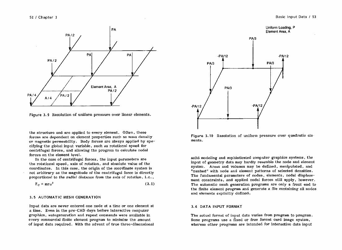
3.4.2 Distributed Forces
Distributed forces such as pressure are almost always input to the program by specifying a range of elements over which the pressure acts, the direction and amplitude of the pressure. The program, in turn, breaks down the pressure into the appropriate nodal forces. When pressure is applied to a surface, the equiva- lent nodal forces are calculated by the product of the node’s share of the area and pressure over that area. Figure 3.8 shows a sim- ple one-dimensional example of a uniform pressure applied over two series of nodes, one with uniform pressure and the second with nonuniform pressure. Note that with the case of uniform pressure, the end nodes only get half the force of the interior nodes. Although this appears to apply a nonuniform force to the model, it does result in the correct pressure distribution.
For linear elements with corner nodes only, the resolution of applied pressure to nodal forces follows a linear pattern, with each node receiving its share of force based on the product of its equivalent area and applied pressure as shown in Figure 3.9. For quadratic elements, with midside nodes, the force resolution scheme is more complex, as shown in Figure 3.10. The force res- olution for the quadratic elements is not intuitively obvious and is the result of the integration of pressure over the element sur- face using the element’s integration functions.
Because forces are applied only at the node points, it is im- possible to achieve a perfectly distributed or continuously vari- able force. As force varies from node to node, it is represented by the element as either a step or linear ramp change. For this reason, stress results in elements with applied nodal forces will not yield the best results. Internal forces and stresses will “even out” within a few layers of elements so that the stresses Will be of normal accuracy within a short distance of the nodal forces. The general rule of thumb is to use a radius of three elements away from the element with the applied force to find good stress results. In areas where each node is carrying the same force, this distance should be less because it is the step changes in applied force that locally affect the stress results. In cases where it is important to calculate stresses near a sur- face with an applied load, several layers of small elements are recommended.
3.4.3 Body Forces
Another class of applied forces is body forces. Included are forces such as centrifugal or magnetic forces that act throughout
Uniform Loading, P Ibfhn Y
t X
Fy =P xA X12
PAX PAX PAX
PA Xl2 PA X/2 Final Nodal Force Breakdown
Figure 3.8 Resolution of pressure loading into nodal forces.
52 I Chapter 3 Basic Input Data / 53
I PA
Figure 3.9 Resolution of uniform pressure over linear elements.
the structure and are applied to every element. Often, these forces are dependent on element properties such as mass density or magnetic permeability. Body forces are always applied by spe- cifying the global input variable, such as rotational speed for centrifugal forces, and allowing the program to calculate nodal forces on the element level.
In the case of centrifugal forces, the input parameters are the rotational speed, axis of rotation, and absolute value of the coordinates. In this case, the origin of the coordinate system is not arbitrary as the magnitude of the centrifugal force is directly proportional to the radial distance from the axis of rotation, i.e. ,
Fc = mrw* (3.1)
3.5 AUTOMATIC MESH GENERATION
Input data are never entered one node at a time or one element at a time. Even in the pre-CAD days before interactive computer graphics, autogeneration and repeat commands were available in every commercial finite element program to minimize the amount of input data required. With the advent of true three-dimensional
Uniform Loading, P Element Area, A
PA/3
I
2
Figure 3.10 Resolution of uniform pressure over quadratic ele- ments.
solid modeling and sophisticated computer graphics systems, the input of geometry data may hardly resemble the node and element system. Areas and volumes may be defined, manipulated, and “meshed” with node and element patterns of selected densities. The fundamental parameters of nodes, elements, nodal displace- ment constraints, and applied nodal forces still apply, however. The automatic mesh generation programs are only a front end to the finite element program and generate a file containing all nodes and elements explicitly defined,
3.6 DATA INPUT FORMAT
The actual format of input data varies from program to program. Some programs use a fixed or free format card image system, whereas other programs are intended for interactive data input
54 I Chapter 3
Table 3.1 Examples of Two Data Input Formats
Parameter
Node definition
ANSYS Msc /NASTRAN
Node 1 at x = 1.00 N, 1, 1, 0, 2 GRID, l,, 1, 0, 2 y = 0.00 z = 2.00
Two-dimensional ele- E. 1, 2, 6, 5 CQUAD4, 1, 1, 2, 6, 5 ment with nodes 1, 2, 6, 5
Displacement con- D, 1, ALL SPCl, 1, 123456, I straint at node 1 with all three D.O.F. constrained
and rely heavily on graphics, incorporating data editing commands along with data input commands. A comparison of two of the more popular programs, ANSYS and MSC /NASTRAN, shows the differ- ent systems for basic data entry (see Table 3.1).
3.7 SUMMARY
A study of modeling principles must be preceded by a knowledge of basic finite-element input data, especially in the case of the novice finite element user. Modeling is actually the optimization of basic input data for a given problem; therefore, a knowledge of what data needs to be optimized is essential. As the data in- put procedures for the various finite element programs grow more sophisticated, they become more removed from the basic input data. Explicit node and element definition is being replaced by line, area, and volume definition and automatic mesh generation. In using the more sophisticated autogeneration routines, the en- gineer must keep in mind the basics of model building in order to develop a cost-effective model and to ensure that the autogenera- tion routines give the appropriate model.
4
PROBLEM DEFINITION
The previous two chapters have given theoretical background in- formation and generic data input requirements for finite element analysis. The objective of this chapter is to give some guidelines for combining the user’s knowledge of the structure or machine component to be analyzed, together with the data input require- ments to form the most cost-effective model that will yield accep- table results. The definition of modeling given here is the pro- cess of examining an engineering problem and developing the most cost-effective set of input data that will help solve the problem.
To put Chapters 2-4 in perspective, an analogy can be made to teaching someone to drive an automobile. The theory discussed in Chapter 2 is analogous to a discussion of the internal combus- tion engine and an explanation of how a transmission and brakes work. These are the under-the-hood details that are not neces- sarily required to operate the automobile, but are recommended for a basic understanding of it. Chapter 3 provides a set of ge- neric data input requirements that are applicable to almost any finite element program. This is analogous to basic automobile
55

56 / Chapter 4 Problem Definition / 57
operation principles. All automobiles are operated in basically the same manner. For example, the brake is operated by a pedal on the floor, etc. In this current chapter, guidelines for the intel- ligent applications of finite element analysis will be given so that the finite element “automobile” travels to its destination in the most direct manner and with the best “mileage.” In driving, no one would drive with one foot on the accelerator and one foot on the brake for any length of time; however, with finite element applications, it is possible to develop a model that will consume l’gallonst’ of computer time without providing the required result.
The optimum model development procedure can be generally broken down into three steps
Problem definition. Free-body diagram. Finite-element model.
The generation of the actual finite element gridwork is the most difficult part of the modeling process and this is what most engi- neers think of when they hear the word “modeling.” This task can be simplified by breaking down the entire modeling process into discrete steps so that the process of gridwork layout can be isolated and handled in an organized manner. Steps 1 and 2, problem definition and the free-body diagram, will be covered in this chapter and finite element model generation in Chapter 5.
Six examples will be used throughout this, and subsequent, chapters to illustrate this procedure: a plate with a circular hole in uniaxial tension, a notched block, a pressure vessel, a welded crank, two gears in contact, and a turbine blade.
4.1 PROBLEM DEFlNlTlON
The problem definition step requires the most nonfinite element experience and should take place before the engineer sits down at the computer terminal. The problem definition step requires a knowledge of the structure to be analyzed and its anticipated behavior. In this step, a number of questions must be answered and the engineer needs to have, at least, a mental checklist of items to be determined and quantified. This list should include, at a minimum, the
Objectives of the analysis. Exact geometric description of the structure. Forces acting on the structure. Displacement constraints acting on the structure.
In determining the objectives of the analysis, the following questions must be answered:
1. What is the specific engineering problem being addressed? It may be a failure of an existing structure, the likelihood of fail- ure of a new prototype structure, the amount of deflection of the structure during operation, or the amount of vibration produced or transmitted by the structure during operation. In many cases, there may be more than one objective to the analysis. The time to determine all the information that will be required from the analysis is at this, first step.
2. What level of accuracy is expected or required from the analysis? Is the purpose of the analysis to provide “ballpark” numbers and general guidance for design or is the analysis of a critical component that must be precisely designed? What will the consequences be if the component or structure fails in the future?
3. What parameters will affect the performance of this struc- ture? Such parameters include static loading and stress, vibra- tion and/or resonance, thermal effects, etc. Does the structure behave in a linear manner or will nonlinear effects such as creep or buckling have to be taken into account? If there are nonlinear effects that cannot be included in the finite-element analysis, how will they affect the final accuracy of the analysis?
The exact geometric description of the component or structure depends not only on design drawings but also on tolerance effects. If an analysis of an existing structure is required, it is important to check the structure against design specifications to make sure that it meets those specifications and to take note of any excep- tions. When tolerances and manufacturing techniques are impor- tant , such as the dynamic stiffness of a bolted joint, it is neces- sary to quantify the range of composite tolerances. Consideration should be given to making several parametric calculations to bracket the tolerance effects.
As part of this step, it is necessary to make a decision as to how much of a structure, machine, or machine component to in- clude in the model. Generally, there are a finite number of areas of interest that are determined from previous experience or as a result of engineering judgment. The decision then is how much of the surrounding structure needs to be included in the model. This is largely dependent on which parameters affect the behavior of the structure and how much confidence the engineer has in anticipating, at least qualitatively, those effects. For example, in the case of vibration, it may be necessary to model the en- tire structure to obtain the dynamic stress at one point because the dynamic response is dependent on the stiffness and mass

58 I Chapter 4 Problem Definition / 59
distribution of the entire structure. The use of symmetry may be considered to reduce the problem size.
Forces acting on the structure can consist of static discrete forces, distributed forces, dynamic transient forces, dynamic harmonic forces, thermal effects, and electromagnetic effects. In this problem definition step, it is necessary to make assump- tions as to which forces to consider and which to ignore. This requires engineering judgment and familiarity with structure and its behavior.
Static forces require quantifying force amplitude and location. Quantifying forces is often related to deciding how much of a structure to include in the model. When forces on one component of a structure or machine are transmitted by another component, it may be necessary to include the second component in the model to get the accurate force distribution on the primary component of interest.
Dynamic forces require (1) force amplitude, (2) location, (3) frequency, and (4) phase angle. For both transient and harmonic forces, there may be more than one time history or frequency in- volved . In these cases, it is necessary to know the time-phasing relationship between the forces. It is also necessary to quantify the damping acting in the structure. Damping is a process of dissipating energy that can consist of three basic mechanisms: (1) material or hysteretic damping due to internal friction in the structure, (2) coulomb or dry friction damping due to sliding be- tween surfaces, and (3) aerodynamic (viscous) damping due to the motion of a structure through a fluid such as an airplane wing or a shock absorber.
Displacement constraints require some assumptions to be made as to a location in the structure, away from the critical areas, that may be assumed to be “rigid.” Although there is no point in any real structure that has no deflection, there are points where the engineer intuitively knows that the deflections will be two or three orders of magnitude lower than the deflections in the critical areas. The decision as to how and where to assume displacement constraints is‘directly related to the decision on how much of the structure is to be modeled and whether or not symmetry can be used to minimize the size of the model. An ideal situation is one of a relatively flexible, isolated component connected to a massive structure by a rigid con- nection, i.e., a bracket welded to a machine frame.
Displacement constraints can be classified into several broad cat- egories : (1) rigid in which all degrees of freedom are constrained along an entire boundary, i. e . , a welded connection. (2) roller in
which displacements are constrained in one or two directions and are free to move in the other direction(s). For example, a loosely bolted connection in which displacements can be constrained be- tween two surfaces in the normal direction but are free to move laterally could be modeled with roller constraints. And (3) gap constraints in which a structure is free to deflect a limited amount before running into a rigid constraint in one or more directions.
In the problem definition step, it is necessary to examine the structure and classify the objectives of the analysis, quantify the size of the model, and classify and quantify the applied forces and displacement constraints. These items can be summarized in a checklist given in Table 4.1.
4.2 EXAMPLE CASES
A set of six example cases are discussed. The cases are arranged in order of increasing complexity. This set of six problems will be used in subsequent chapters to illustrate the modeling process. In this problem definition stage, the problem statement is somewhat arbitrary, so for each case, there could be multiple problem state- ments, each of which could lead to a different model of the same structure.
4.2.1 Example: Plate with Circular Hole
A simple plate, in uniaxial tension, with a circular hole is shown in Figure 4.1. In this, the simplest case, the model will be from a textbook problem rather than a “real world” practical case. An exact solution exists for the stress field that will allow for com- parison with finite element results. The solution used for com- parison here is taken from Seeley and Smith [l] .
In the case of the plate with the circular hole, the checklist of Table 4.1 can be followed to define the analysis.
1. Objectives The problem is to solve for the maximum static stress in the plate to within 10% of the true value. Although this is an example problem, it must be assumed that thermal effects can be neglected and only the applied static forces will affect the stresses.
2. Exact geometric description Because this is a simplified example problem, it may be assumed that the nominal dimensions given in Figure 4.1 may be accepted as shown. Tolerance effects will not be included. It can be seen that because of the assumed

60 I Chapter 4
Table 4.1 Problem Definition Checklist
Problem Definition I 61
Uniform In-Plane Tension on Opposing Edges
1. Objectives 1.1 What is the problem to be solved? 1.2 What level of accuracy is to be expected? 1.3 What are the parameters that can affect the behavior of
the structure?
2. Exact geometric description 2.1 Are drawings of the structure available? 2.2 Does the actual structure conform to the drawings? 2.3 What are the manufacturing tolerances specified for the
structure and what tolerances are actually expected? 2.4 What unspecified effects of tolerance and fit can affect
the behavior of this structure? 2.5 How much of the structure needs to be included in the
finite element model? 2.6 Can symmetry be used to reduce the size of the model?
3. Forces 3.1 What types of forces act on the structure: static, dy-
namic, or thermal? 3.2 What is the location and magnitude of these forces? 3.3 For dynamic forces, what are the frequencies and phase
angles of the forces and what is the damping in the struc- ture?
3.4 For thermal cases, are the temperature distributions known or will a thermal finite element analysis be re- quired to obtain the temperatures?
4. Constraints 4.1 What types of constraints are present: rigid, roller, or
gap ? 4.2 At what locations can constraints be assumed to be ap-
plied? 4.3 For gap-type constraints, what is the limit of deflection?
uniform force, only one-quarter of the plate needs to be included in the model. A quarter-symmetric model is adequate to represent the plate because the stress distribution in each of the quadrants will be mirrored about the planes of symmetry. If the force was nonuniform, then a half-symmetric or full-plate model would need to be used.
f/l = 100.0 IbWin.
Plate of Uniform Thickness t = 0.1 in.
Overall Dimensions
Uniform Tension 100 Ibf/in.
Figure 4.1 Plate with circular hole: Problem definition.
3. Forces The only forces shown in Figure 4.1 are in-plane forces uniformly distributed over the two ends. Therefore, a two-dimensional plane stress model will be sufficient. Obviously, the total forces on each end must be equal for the plate to be in equilibrium.
4. Constraints To maintain equilibrium and proper displace- ments, roller constraints should be specified along the symmetric, cut boundaries. Along the X axis cut boundary, displacements should be constrained in the Y direction, but the surface should be free to move in the X direction. A similar situation holds for the Y axis cut boundary where the X direction should be con- strained and the Y direction free to move.
The use of the quarter-symmetric model with force on one face and roller constraints on the symmetric boundaries will elimi- nate the problem of trying to apply perfectly balanced forces to the finite-element model. Due to computer truncation and round- off error, it is practically impossible to input sets of forces that will balance and not result in a net force.

62 I Chapter 4 Problem Definition / 63
4.2.2 Example: Notched Block
A simple block with a notch is shown in Figure 4.2. This is, again, a simplistic example but it serve? to illustrate the model- ing process. Two force cases can be considered, uniform ten- sion and a tensile gradient across the end faces.
A review of the checklist of Table 4.1 might yield the follow- ing:
1. Objectives The problem is to solve for the maximum static stress in the block. It will be assumed that thermal effects may be neglected. Only the applied static force, as shown in Figure 4.2, will be considered.
2. Exact geometric description The dimensions of the block given in Figure 4.2 will be accepted as shown. A half-symmetric model will be formed from the block. A quarter-symmetric model could be formed but it would place the location of anticipated max- imum stress at the base of the notch, along a cut boundary. Be- cause the geometry of this example is more complex than the plate
Overall Dimensions of 1 .OW x 3.25H x 2.00
Figure 4. 2 Notched block: Problem definition.
Block with Deep Notch onSides 0.08 Circular Arc Radius at Bonom of Notches
Top and Bonom Surfaces
with the circular hole, it was decided not to use a quarter-sym- metric model. The force profiles are symmetric about the center plane so that the force is not a consideration in the decision as to what type of symmetry may be used.
3.. Forces The forces shown in Figure 4.2 are uniaxial tensile forces. Two cases are shown. The first is a uniform distribution and the second is a nonuniform distribution, symmetric about the center plane. For the first case, a two-dimensional model would be adequate. Because the block is fairly deep, a plane-strain model will be used. In the case of the nonuniform force distribu- tion, a two-dimensional model would give an approximation of the true stress. However, a full three-dimensional model will also be used.
4. Constraints Roller constraints will be used along the cen- ter plane of symmetry. To prevent numerical problems, con- straints will be applied to the bottom surface of the block, in lieu of an equal and opposite set of applied forces. Along the bottom face, roller constraints will be applied in the vertical direction. The surface will be free to move in the two, in-plane directions. One point on the block will have to be constrained, normal to the plane of symmetry to prevent rigid body motion of the block.
4.2.3 Example : Pressure Vessel
A simple pressure vessel is shown in Figure 4.3. The pressure vessel has an internal pressure of 100.0. The pressure vessel can be considered to be a solid of revolution about its axis and symmetric about a center plane, normal to its axis.
1. Objectives To solve for the maximum static stress in the pressure vessel due to the internal pressure force. In this ex- ample, thermal effects will be ignored. This example will be mod- ified in Chapter 12 to illustrate the inclusion of thermal effects.
2. Exact geometric description The dimension as shown in Figure 4.3 will be used as shown. In a real pressure vessel, the locations of welds should be noted to see if they could cause a geometric discontinuity in the structure. Lifting lugs and ex- terior attachment points would also have to be noted. This pres- sure vessel will be modeled as an axisymmetric structure. The center plane of symmetry will be used to model only half of the pressure vessel.
3. Forces Internal pressure will be the only applied force. Other forces that could also be considered under certain circum- stances are gravity force and reaction forces at support points. Fluid dynamic forces, either gas or liquid, could also be taken

64 I Chapter 4 Problem Definition / 65
ID= 10.0 OD= 11.0 Wall Thickness = 0.50
1
----__ / -.--- -_
/
i 7 f
‘\ \ R = 3.75 1
I Internal Pressure = 100.0
I - -
I I
\ I \ /
\ / c------- ____-_ 4
Symmetric About Centerline and Center Plane
Figure 4.3 Pressure vessel: Problem definition.
into account in the event of any agitation or reaction of the ves- sel’s contents. These internal forces, if they are applicable, are more difficult to quantify and require a detailed understanding of the process taking place within the vessel.
4. Constraints The only constraints that need to be applied are roller constraints in the axial direction along the cut center plane of symmetry. Because this is an axisymmetric model, con- straints in the radial direction are not required so long as the boundary at the centerline has a radial coordinate of 0.
4.2.4 Example: Crank
The hand crank is a welded machinery component as shown in Fig- ure 4.4. A handle is connected to one end of the crank through a 0.625 reamed hole and a shaft is connected to the other end, and torque is transmitted by a square key. Hubs at each end of the crank are welded to a baseplate.
Shaft
Handle
Figure 4.4 Crank: Problem definition.
1. Objectives The objective of the analysis is to determine the maximum stress at the keyway (the point of maximum antici- pated stress) as a function of transmitted torque. Once again, thermal and dynamic effects will be neglected. It will be arbi- trarily decided that the only part of the assembly to be consid- ered will be the crank. Stresses in the shaft will not be calcu- lated in this example.
2. Exact geometric description From an examination of the detailed part drawings, it is determined that the handle is at- tached to the crank with a light interference fit (0.0002-0.0010 tight). From this, it may be assumed that, there is complete con- tact between the handle and crank. At the shaft end, the fit be- tween the shaft and crank bore is from 0.0005-0.0010 loose. Therefore, in a worse-case situation one would have to assume that there is no torque transmitted due to friction between the crank and shaft and that all the torque is transmitted by the

66 I Chapter 4 Problem Definition / 67
key. The key is a tight fit in the shaft and a loose fit (0.0002- 0.0008 loose) in the crank. Because the crank only transmits force in one direction of rotation, it may be assumed that there is complete contact between the driving side of the key and the corresponding side of the keyway. It may be further assumed that because the crank does not alternate directions, there will be no impact-type force between the key and keyway.
3. Forces Applied forces will consist of the torque force ap- plied as a linear distributed force at the handle.
4. Constraints Displacement constraints are applied at the shaft lkeyway area of the crank. Local radial constraints are applied around the inside of the bore of the crank to prevent deformation, but not to transmit any torque. Local tangential constraints are applied to one edge of the keyway to obtain ap- propriate reaction forces.
Although this could be approximated as the two-dimensional problem, a full three-dimensional model will be formed. It is not intuitively obvious whether or not there will be a force gradient along the length of the keyway. The highest force may be trans- mitted at the base of the crank where the plate attaches to the hub. However, this area has the most reinforcement due to the plate so that the highest stresses may not necessarily occur there. For that reason, a full three-dimensional model of the crank will be used. The handle, shaft, and key will not be in- cluded in the model.
4.2.5 Example: Gear Segment
This example problem may be approached from a number of dif- ferent directions with various objectives and levels of accuracy desired. The gears to be modeled are shown in Figure 4.5. They are a pair of straight spur gears with a 20° pressure angle and a dimetral pitch of 2. Both the diving and driven gear have 40 teeth each and, therefore, operate on a pitch diameter of 20.0. All other dimensions are standard for full-depth teeth of this pitch and pressure angle.
Various options for modeling from the simplest to the most complex might be the following:
Two-dimensional model of a single tooth with applied forces. Two-dimensional model of a segment of teeth with applied
forces. This would allow for the interaction of the forces on adjacent teeth to be more correctly accounted for in the fillet area between the teeth.
Straight Spur Gears
Pitch Dia. = 20.0
Pressure Angle = 20 degrees
Number of Teeth (Each Gear) = 40
Figure 4.5 Two gears in contact: Problem definition.
Two-dimensional model of two segments, one of the driving gear and the other of the mating, driven gear, with gap elements between the contacting profile surfaces to allow the force between the teeth to be more correctly distributed by the model.
Three-dimensional model of a single tooth with applied contact pressure distribution to be applied. This would allow for a variation in contact pressure and stress along the length of the tooth.
Three-dimensional model of a segment of teeth. Three-dimensional model of contacting segments of driving and
driven gears with gap elements in between mating tooth SW- faces. This would allow for lengthwise’variation in contact due to “crowning” of the teeth. Because the force between

68 I Chapter 4 Problem Definition / 69
the teeth is constantly changing as the teeth roll through contact, a segment model of this type should be incremented to simulate a stress time history.
Three-dimensional model of driving and driven segments with allowance for mounting errors and mounting flexibility. There is normally some flexibility associated with the gear mountings and bearings that can cause the contact pattern to shift and thereby change the pressure and stress distribution.
The purpose of listing the above options is not to confuse the matter, but to illustrate some of the thinking that must take place long before the actual finite element modeling begins. In this gearing problem, there are more approaches to the problem than in the previous cases. There is obviously no one “cookbook” method of modeling a gearing problem.
All of the above models are for static deflection and stress analysis. Thermal effects are generally not considered to be sig- nificant in gearing problems except in unusual circumstances. Dy- namics are taken into account in the event of a resonance condi- tion of the gear drive system, either lateral or torsional, excited by a harmonic of the running speed of one of the gears or by the gear set’s tooth mesh frequency.
1. Objectives There may be one of several objectives to the analysis, each of which may require a different type of model. The two most common objectives of gearing analysis are the de- termination of root fillet bending stresses that can lead to fatigue or the determination of profile contact stresses that can lead to spalling or pitting. For the present purposes, the objective will be to obtain the root fillet cyclic bending stresses.
2. Exact geometric description All dimensions such as adden- dum , dedendum , etc. will be for standard 20° pressure angle, 2 pitch spur gears with 40 teeth. No lengthwise crowning or pro- file modifications will be assumed. The teeth will be assumed to have a perfect involute shape with circular arc fillets and no un- dercut in the fillet.
Stress analysis of gear teeth can be quite complex. A number of simplifying assumptions are made here. However, this type of problem description and model should be quite adequate to rep- resent first-order effects and give a result equal to or better than conventional closed-form solutions.
4.2.6 Example: Turbine Blade
This example case is a steam turbine blade from a low-pressure stage of a large power-generation turbine as shown in Figure 4.6.
A typical analysis for a blade of this type would include a static stress calculation, natural frequency and mode shape calculation, and possibly a calculation of dynamic stresses.
Most of the static stress in the blade is from centrifugal force, due to the blade rotating at 3600 rpm. Steam forces are typically two orders of magnitude less than the centrifugal forces. Steam forces may be in the 100-300 lbf range, whereas the centrifugal force may be lO,OOO- 30,000 lbf at the base of the blade.
There are several parts to a turbine blade. The airfoil section of the blade is tapered and twisted with highly curved surfaces. The turbine blade is sensitive to the interaction of its natural frequencies with harmonics of the running speed. Therefore, it is important to correctly calculate the natural frequencies, which, in turn, requires an accurate geometric model of the airfoil sec- tion . In some cases, the blades are independent of each other, i.e., freestanding. In other designs, the blades are connected at their tips into groups of three to seven, typically. The blades are grouped for dynamic stiffening to minimize dynamic response and also to provide a sealing surface to prevent steam leakage. The cover is attached to the blade group by a cold rivet, known as a tenon that is integral with the airfoil. As may be expected, the junction of the tenon with the top of the airfoil is an area of highly localized stress, especially when the residual riveting stresses are included. The blade is, attached to the rotor by a slotted, “firtree”-type construction so that each blade fits into a precisely machined slot in the rotor. The attachment region of the blade has high, localized, static stresses in the t’hooklt notches. In these areas, specification of the appropriate contact between the blade hooks and rotor serrations is important to the calcula- tion of local stress that may approach or equal the yield strength of the material.
1. Objectives The objective of this study is to calculate the maximum static stress in the blade under steam loading and at operating speed. Any consideration of dynamic effects will be deferred to Chapter 11. Thermal effects will not be considered here. This low-pressure blade operates at 150°F nominally with changes of f20°F.
2. Exact geometric description Dimensions are critical in two areas : The first is the blade/rotor attachment areas where there are six contact surfaces. Due to a buildup of tolerances, there may occur conditions when all six surfaces are not in contact and only three or four surfaces are carrying the load. If the surfaces are slightly out of contact, i.e. ,within 0.001 in., then elastic de- formation will pull the out-of-contact surfaces into contact. Even so, the notches associated with the surfaces originally in contact

70 / Chapter 4
Figure 4.6 Above: Turbine blade; problem definition. Opposite, top: Turbine blade; showing cover e.rea. Opposite, bottom: Tur- bine blade, showing root attachment area.
Blade Root Attachment Area Rotor Segment Not Shown

72 I Chapter 4 Problem Definition / 73
will see a higher stress than notches associated with surfaces in- itially out of contact. In this area, the exact geometry may be obtained from the detail part drawings that include the profile tolerances or from measurements of the actual blade and rotor slot.
The second area is the airfoil profile. This is important in the calculation of natural frequencies and dynamic response, but not as important in the calculation of static stresses. Again, the profile description, generally in terms of coordinates at a number of cross sections, may be obtained from the manufacturing draw- ings or from the actual blade.
3. Forces Two types of forces are applied to the turbine blade, the centrifugal force and steam forces. Centrifugal forces will be calculated automatically by the finite-element program so that the only input parameter that needs to be defined is the ro- tational speed. Dimensions of the blade must be defined in terms of their absolute distance from the rotor centerline, the center of rotation. So long as the geometry input and material density are properly specified, the centrifugal body forces will be correctly calculated and applied in the finite-element model. The applied steam forces may be applied either as a distributed pressure force across the airfoil or, in this case, resolved into tangential and axial force components based on force distributions in the two di- rections and distributed across the appropriate airfoil nodes.
4. Constraints Because the areas of anticipated highest stress are in the firtree attachment, a section of the rotor surrounding the blade attachment is included in the model. Displacement con- straints are applied at the outside boundary of the rotor segment. The contact surfaces of the blade and rotor are coupled.
This is an obvious case for a full three-dimensional model. The use of a two-dimensional refined model in the attachment area will be discussed in Chapter 10.
4; 3 FREE-BODY DIAGRAM
As an intermediate step following the problem definition and before actual model coding, it is advisable to construct a free-body dia- gram of the portion of the structure that is to be included in the model. This free-body diagram should show applied forces and displacement constraints in the same location, direction, and mag- nitude as they will be applied to the finite-element model. The construction of the free-body diagram allows for a check on those
items such as forces and constraints that need to be quantified prior to model coding. Because forces and displacements can only be applied at nodes, it is necessary to have the locations of all forces and displacements identified prior to model generation to insure that nodes are positioned correctly. With modern CAD and solid modeling software, it is possible to create a free-body diagram within the computer. Otherwise, it is necessary to cre- ate the free-body diagram on paper that can then be copied as many times as necessary for the next step, gridwork develop- ment , and coding.
4.4 FREE-BODY DIAGRAM: EXAMPLE CASES
4.4.1 Example : Plate with Circular Hole
A free-body diagram for the plate with a circular hole is shown in Figure 4.7. The diagram shows the quarter-symmetric por- tion of the plate. The diagram is shown as a two-dimensional representation of the plate because there are no out-of-plane forces and should not be any out-of-plane displacements. Roller constraints are specified along both the cut boundaries. Along
Roller Constraints
b (1 0 0 0 0 0 (
- Distributed Loading
Quarter-Symmetric
--w 2D Model - No Out-of- Plane Forces
Symmetric Boundaries
Figure 4.7 Plate with circular hole: Free-body diagram.

74 1 Chapter 4 Problem Definition / 75
the X axis, it is necessary to allow motion in the X direction be- cause of the applied force in that direction. Along the Y axis, there should be no displacement in the X dii+ection because of the balanced forces and assumption of symmetry. There will be displacement in the Y direction along the Y axis due to Poisson’s effect as the plate becomes narrower due to the tension in the X direction. The applied force is shown as a uniform force distrib- uted along the right-hand edge of the plate acting only in the X direction.
4.4.2 Example: Notched Block
The free-body diagram of the notched block is shown in Figure 4.8. The diagram shows a half-symmetric representation of the
Distributed Loading
3 Roller Constraints
Half-Symmetric Model
Roller Constraints
Figure 4.8 Notched block: Free-body diagram.
block with roller constraints along the plane of symmetry constrain- ing against out -of-plane deformation. Roller constraints are also shown on the bottom surface of the block opposite the end of the applied force. These roller constraints arise in lieu of applying an equal and opposite force distribution.
A distributed force is applied across the top of the block. Be- cause the force distribution is constant in the Y direction, the use of symmetry is acceptable.
4.4.3 Example : Pressure Vessel
The free-body diagram for this axisymmetric model is shown in Figure 4.9. Because of the symmetry about the midplane, only half of the pressure vessel is included in the model. Roller con- straints to prevent against deformation in the axial direction are used on the cut plane. No constraints are required for the radial direction for an axisymmetric model. A uniform internal pressure is applied to the entire inside surface of the pressure vessel.
4.4.4 Example: Crank
In modeling the crank, it was decided to only include the crank itself in the model and not the handle, shaft, or key. The free-
Rofler Constraints
Distributed Pressure Loading P E 100.0
Axisymmelric Model
NO Radial Constraints Necessary for Ax~symmetric Problem
Figure 4.9 Pressure vessel: Free-body diagram.

76 I Chapter 4 Problem Definition / 77
body diagram of the crank is shown in Figure 4.10. Displacement constraints are applied at the inside of the shaft bore to represent the reaction of the shaft and key. The effect of the shaft is rep- resented by allowing displacement in the local tangential direction on the inside of the shaft bore, but constraining against any dis- placement in the local radial direction. The key is represented by displacement constraints on the side of the keyway in the tan- gential direction. The handle is represented by applied forces at the inside of the handle bore. Symmetry cannot be used here to reduce the model size due to the axisymmetric location of the key- way.
An alternative free-body diagram would include the shaft and key. This would require, however, the use of gaps between the separate components, which causes the problem to become non- linear and substantially increases the computer runtime.
4.4.5 Example: Gear Segment
The gear segment is shown as two free-body diagrams. The two diagrams are shown in Figure 4.11 for a single tooth and in Fig- ure 4.12 for a three-tooth, driven-gear segment. If we assume
Only the Crank Is included in the Free-Body Diagram
Key in the Keyway Distributed Loading to Represent the Handle
Figure 4.10 Crank: Free-body diagram.
Distributed Loading Along Pressure Side of Tooth Profile
Roller Constraints Along Cut Boundaries
Figure 4.11 Single gear tooth: Free-body diagram.
that there is no lengthwise curvature (crowning) of the teeth, then the free-body diagrams apply to either the two- or three- dimensional cases.
The free-body diagram of the single tooth shown in Figure 4.11 show’s a force distribution on the pressure side of the tooth profile. Displacement roller constraints are applied at the base

78 I Chapter 4
Roller Constraints Along Cut Boundaries of Driven Gear
Figure 4.12 Three-tooth gear segment: Free-body diagram.
of the tooth in the radial direction. Roller constraints are also applied to the sides of the tooth along the cut boundaries be- tween the teeth in the tangential direction.
The free-body diagram for the three-tooth segment shows distributed forces across the pressure faces of the three teeth. Displacement constraints are applied to the cut boundaries of the driven gear. Roller constraints are again applied at the bottom of the segment in the radial direction. Roller constraints in the tangential direction are applied at the cut boundaries of the first and third driven gear teeth in the tangential direc- tion.
4.4.6 Example: Turbine Blade
The free-body diagram for a grouped turbine blade is shown in Figure 4.13. The free-body diagram consists of the blade air- foil, integral tenon, a portion of the cover, root attachment, and a segment of the mating rotor including the rotor slot into which the blade fits. The portion of the cover was included in the free- body diagram in order to provide the proper centrifugal force to the tenon and so as not to require specifying boundary conditions directly at the highly stressed tenon. The rotor segment is in- cluded in the model for a similar reason: To eliminate the need to apply assumed boundary conditions at the load-bearing sur- faces of the root hooks.
Problem Definition / 79
Centrifugal Body Forces
Cover - Roller Constraints Along Cut Boundaries
Distributed Steam Forces
Roller Constraints Along Cut Boundaries of Rotor Segment
Fully Coupled Contact Between Blade and Rotor Contacting Surfaces
Figure 4.13 Turbine blade: Free-body diagram.
Applied forces consist of a distributed force in the tangential and axial directions along the airfoil section representing the ap- plied steam forces. Displacement constraints are applied at the

80 I Chapter 4
cut boundaries of the rotor segment with roller constraints in the radial direction and along the side of the rotor segment in the tan- gential direction. The contact surfaces between the blade root and rotor are assumed to be coupled.
4.5 SUMMARY
The process of forming a finite element model can be made more straightforward by clearly defining the problem prior to sitting down at a computer terminal and entering input data. This chap- ter covers steps 1 and 2 of a three-step procedure for developing a model. Step 1 involves defining the engineering problem and objectives of the analysis. Step 2 involves a decision on how much of the structure to include in the model and how much can be cost-effectively included in the model. Step 2 also covers the specification of boundary conditions. Once these two steps have been completed, the actual development of the finite element model may proceed in an organized manner. Time spent in defining and specifying the analysis will pay dividends later on in the actual finite element calculations and data analysis.
REFERENCE
1. Seeley , F. B. and J. 0. Smith, Advanced Mechanics of Ma- terials , 2nd ed. , Wiley, New York, 1932.
5
FINITE ELEMENT MODEL
Once the problem has been defined and the free-body diagram constructed, the development of the finite element gridwork, coding, and entering the model into the computer consist of (1) dividing the free-body diagram into elements, (2) applying forces to nodes, and (3) applying displacement constraints to nodes. Of the three tasks, division of the free-body diagram into elements is by far the most difficult and at the heart of the modeling pro- cess. The specification of applied forces and displacement con- straints should be virtually automatic if the free-body diagram is correctly prepared.
This process of actually creating the finite element gridwork with boundary conditions and entering the data into the computer used to be a multistep procedure. First, the gridwork was laid out on paper; next, lists of the nodes, elements, and boundary conditions were prepared; the input data were either keypunched onto punch cards or entered into a data file; and check runs were made to look for coding and data input errors. With the use of
81
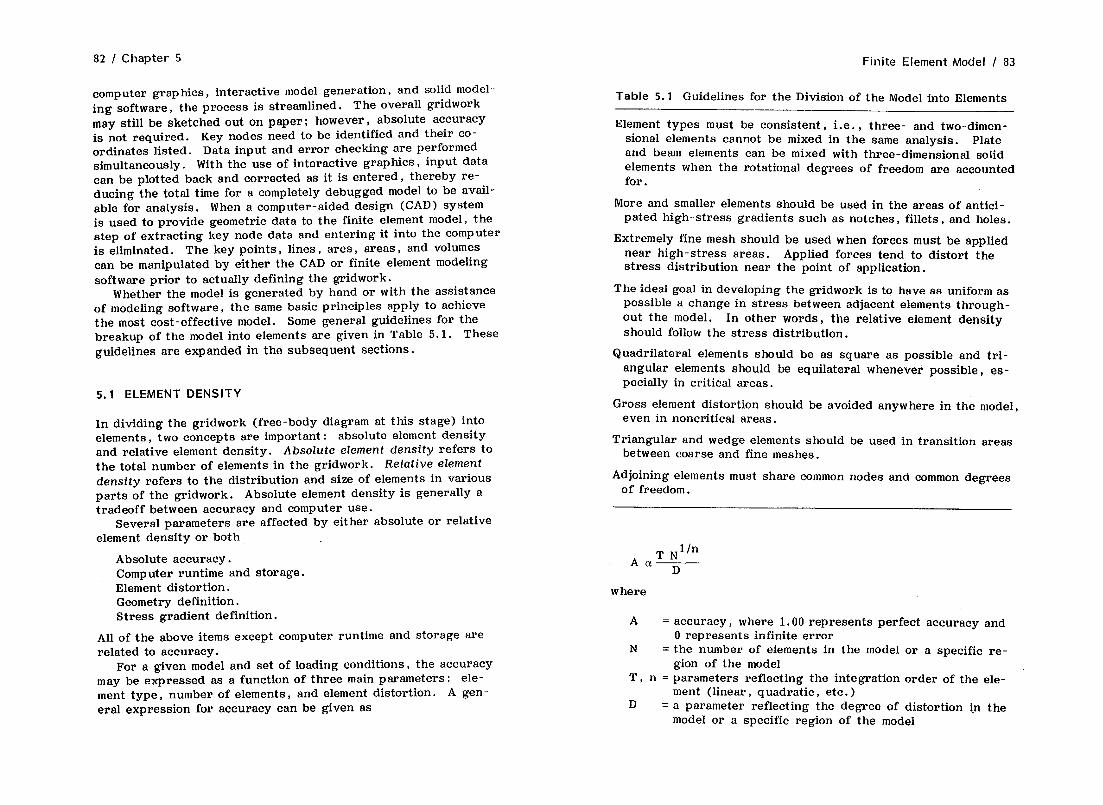
82 I Chapter 5
computer graphics, interactive model generation, and solid model- ing software, the process is streamlined. The overall gridwork may still be sketched out on paper; however, absolute accuracy is not required. Key nodes need to be identified and their CO-
ordinates listed. Data input and error checking are performed simultaneously. With the use of interactive graphics, input data can be plotted back and corrected as it is entered, thereby re- ducing the total time for a completely debugged model to be avail- able for analysis. When a computer-aided design (CAD) system is used to provide geometric data to the finite element model, the step of extracting key node data and entering it into the computer is eliminated. The key points, lines, arcs, areas, and volumes can be manipulated by either the CAD or finite element modeling software prior to actually defining the gridwork.
Whether the model is generated by hand or with the assistance of modeling software, the same basic principles apply to achieve the most cost -effective model. Some general guidelines for the breakup of the model into elements are given in Table 5.1. These guidelines are expanded in the subsequent sections.
5.1 ELEMENT DENSITY
In dividing the gridwork (free-body diagram at this stage) into elements, two concepts are important : absolute element density and relative element density. Absolute element density refers to the total number of elements in the gridwork. Relative element density refers to the distribution and size of elements in various parts of the gridwork. Absolute element density is generally a tradeoff between accuracy and computer use.
Several parameters are affected by either absolute or relative element density or both
Absolute accuracy. Computer runtime and storage. Element distortion. Geometry definition. Stress gradient definition.
All of the above items except computer runtime and storage are related to accuracy.
For a given model and set of loading conditions, the accuracy may be expressed as a function of three main parameters: ele- ment type, number of elements, and element distortion. A gen- eral expression for accuracy can be given as
Finite Element Model / 83
Table 5.1 Guidelines for the Division of the Model into Elements
Element types must be consistent, i.e., three- and two-dimen- sional elements cannot be mixed in the same analysis. Plate and beam elements can be mixed with three-dimensional solid elements when the rotational degrees of freedom are accounted for.
More and smaller elements should be used in the areas of antici- pated high-stress gradients such as notches, fillets, and holes.
Extremely fine mesh should be used when forces must be applied near high-stress areas. Applied forces tend to distort the stress distribution near the point of application.
The ideal goal in developing the gridwork is to have as uniform as possible a change in stress between adjacent elements through- out the model. In other words, the relative element density should follow the stress distribution.
Quadrilateral elements should be as square as possible and tri- angular elements should be equilateral whenever possible, es- pecially in critical areas.
Gross element distortion should be avoided anywhere in the model, even in noncritical areas.
Triangular and wedge elements should be used in transition areas between coarse and fine meshes.
Adjoining elements must share common nodes and common degrees of freedom.
AoTN l/n
D
where
A = accuracy, where 1.00 represents perfect accuracy and 0 represents infinite error
N = the number of elements in the model or a specific re- gion of the model
T, n = parameters reflecting the integration order of the ele- ment (linear, quadratic, etc. )
D = a parameter reflecting the degree of distortion in the model or a specific region of the model

84 I Chapter 5 Finite Element Model / 85
The parameters T and n adjust for the fact that higher-order elements, such as quadratic elements with midside nodes, may achieve the same accuracy using fewer elements as linear Strfdn
elements with more elements. All models, regardless of what kind of elements are used, should asymptotically approach almost per - feet accuracy as the number of elements approaches infinity. Therefore, the effect of higher-order elements may be more pro- nounced for models in which there are fewer elements. Proper- ties of various common element types and rates of convergence are discussed more thoroughly in Chapter 7. As an example, however, the convergence of two triangular, two-dimensional elements is shown in Figure 5.1. The model is a simple canti- lever beam in bending. The two elements are a three-node linear displacement, constant strain triangle and a six-node quadratic displacement, linear strain triangle. It can be seen that for a few elements, there is a significant difference in the accuracy of the two elements, but both elements converge to about 0.98-o. 99 accuracy with more than 50 elements. It must be noted that this simple comparison does not account for computer runtime in which the higher-order more powerful elements require more computer use per element.
The accuracy of the model increases with the number of ele- ments for several reasons.
1. The structure% geometry can be more accurately defined with more points. This is especially true when a curved bound- ary is modeled with linear elements having nodes only at their vertices. These elements must represent the curved boundary as a series of straight lines.
2. Stress gradients can be more accurately defined by having more elements, thereby minimizing stress gradients within ele- ments. This is especially important for linear, constant strain elements.
3. More elements generally means smaller elements close to a fillet or notch surface where a maximum stress may occur. Smaller elements means that the centroids of the surface elements will be closer to the structure% surface simply because of the element size. More elements in these regions give more definition of stress gradients .
When a structure has a simple shape and simple loading, the number of elements may not have any real effect of accuracy. In the simplest cases, almost perfect accuracy can be achieved with one element. Of course, the model has to match exactly the as- sumptions and type of analysis built into the element. For ex- ample, one beam element should give virtually perfect correlation
Act
800%
B5%
SO%
@5%
Bo%
%5%
FO%
0%
:uri A
‘1 c
=Y Accuracy Versus Total Number of Elements - Uniform Cantilever Beam in Bending
3-Node Linear Triangle
I I I
10 20 I
30 I
40 I
50 I b
60 Elements
Figure 5.1 Convergence of two triangular element types.
when compared to a closed-form solution from conventional beam theory. In the same way, a two- or three-dimensional solid element in simple tension with the appropriate boundary conditions should also give perfect results. Due to computer truncation error, it is never possible to have “perfect” agreement t However, perfect or “almost perfect” accuracy can be interpreted as being agreement to five or six significant figures.

86 I Chapter 5
5.2 ELEMENT DISTORTION
Element distortion is given in this chapter as a single parameter; however, its effect on accuracy is complex. The quantitative effects of distortion depend on the type of element, geometry of the structure, type of loading, and specific type of distor- tion . Chapter 8 is devoted entirely to the topic of element dis- tortion.
Element distortion can often be reduced simply by using more elements in part of a model, i.e. , higher relative element den- sity. Quite often, unacceptable element distortion is the result of trying to have a fine gridwork in one part of a model and reducing too quickly to a coarse gridwork in the noncritical areas. This can be resolved by adding more elements in the noncritical areas, thereby reducing the difference in the rela- tive element density.
Examples of gross element distortion that must always be avoided are illustrated in Figure 5.2. The types of distortion shown would cause a fatal error in virtually any finite-element program.
5.3 BOUNDARY CONDITIONS
The specification of displacement boundary conditions is straight- forward if they have been specified on the free-body diagram. In generating the gridwork, node locations may have to be ad- justed and additional nodes and elements added to have nodes available for constraints to be applied at the proper location. Nodes must be positioned at the locations along the boundary that correspond to constraint locations in the actual structure. It is never acceptable to move a constraint to match a node; rather, the node must be located to match the actual constraint.
The specification of applied forces follows the same basic rules as constraints with respect to node location. Forces should be transferred from the free-body diagram to the appropriate nodes and degrees of freedom. Where there are distributed pressure- type forces, the distribution rniy be input directly, if the pro- gram will allow it, or the equivalent nodal forces must be cal- culated according to the rules given in Chapter 3. As men- tioned above, when stresses near a location of applied force are of’interest, it may be necessary to use several layers of small elements in the area to get a reasonable resolution of the lo- calized stresses.
Finite Element Model / 87
Elements Should Never Double back on Themselves
An Element Corner Should Never Collapse to 180 Degrees
3 4
X Element Numbering Must Be Either Clockwise or Counterclockwise
/ \ 1 2
Figure 5.2 Examples of gross element distortion.
5.4 FINITE ELEMENT MODEL: EXAMPLE CASES
For the following examples, data on computer runtimes for the various models are presented. These runtimes are dependent on the computer hardware and finite element software being used. Therefore, the data are presented for a relative comparison be- tween the various models within an example case and between ex- ample cases.

88 I Chapter 5 Finite Element Model I 89
Coarse Gridwork 12 Elements No Attempt Made to Optimize Gridwork
Figure 5.3 Plate with circular hole: Case 1 gridwork.
5.4.1 Example : Plate with Circular Hole
Figure 5.3 shows the first, coarse gridwork generated for the plate with circular hole. Because this is a thin plate and has been determined to be a two-dimensional problem, two-dimen- sional plane stress elements are used.
It is anticipated that the highest stresses and highest stress gradient will occur at the edge of the hole at the X = 0 location. The smallest elements are located around the boundary of the hole. These nodes and elements can be easily generated by de- fining a local, cylindrical coordinate system with its origin at the
center of the hole. Along the Y axis, close to the point of high- est anticipated stress, it is quite easy to have uniform elements. A total of 12 elements are used in this coarse grid model.
The stress and stress gradient can be anticipated by using a closed-form solution [ll to the problem; this gives the stress in the vicinity of the hole as
where
o = the radius of the hole x = the distance from the center of the hole
(5.1)
The maximum stress is then 3~. Forces are applied to the nodes along the right-hand end in
the manner prescribed by the free-body diagram described in Chapter 4. The corner node receives half of the force of the other nodes. Note that the node at the X axis receives the same force as the others because it is assumed that the distributed force is continuous along the right-hand edge.
Constraints are specified at the nodes along the cut bound- aries. Along the X axis, nodes are constrained in the Y direc- tion only, and along the Y axis, nodes are constrained along the X axis only.
The result of the first calculation compared to the closed-form maximum stress is
Finite element maximum centroidal normal stress = 130 psi Finite element maximum nodal stress = 191 psi Closed-form calculated maximum normal stress = 300 psi
To test the sensitivity of the calculation to element density, a second and third calculation are performed with the gridworks shown in Figures 5.4 and 5.5. For the second case (fine mesh) , 132 elements were used. In the third case (selective mesh), 84 elements are used. In the third case, the total number of ele- ments is less than for the second case; however, the relative (local) element density around the hole is about the same. Forces and constraints are specified in a manner similar to that of the first calculation.
The results of the calculations performed with the three mod- els are shown in Table 5.2, along with a comparison of accuracy and computer runtime. These results can also be shown graphi- cally in Figures 5.6-5.8. These results show that although the

90 I Chapter 5 Finite Element Model / 91
Fine Gridwork 132 Elements High Element Density Throughout
Figure 5.4 Plate with circular hole: Case 2 gridwork.
second case had the highest number of elements, the third case had equal accuracy when the elements were concentrated around the hole. In this case, the accuracy is defined as the ratio of maximum stress around the hole to the closed-form calculated maximum, 300 psi.
5.4.2 Example: Notched Block
A total of three separate finite-element models are generated for this example. In section 4.4.2, the two free-body diagrams, two-dimensional and three-dimensional, are discussed. One two-
Optimized Gridwork 84 Elements High Element Density Near Hole Reduced Element Density away from Hole
Figure 5. 5 Plate with circular hole: Case 3 gridwork.
dimensional finite element model is constructed and shown in Fig- ure 5.9, and two three-dimensional finite-element models are con- structed and shown in Figures 5.10 and 5.11. The two-dimen- sional model contained 38 plane strain elements. The coarse three- dimensional model contained one layer of 24 three-dimensional solid elements and the fine three-dimensional model contained two layers of 38 elements (the same pattern as in the two-dimensional model) for a total of 76 elements. The details of the three models and their computer runtimes are given in Table .5.3.

92 I Chapter 5
Table 5.2 Results of Plate Calculations
Case 1 Case 2 Case 3 coarse fine intermediate
Centroid location from edge of hole
Normal stress at cen- troid
Exact solution stress at centroid location
Nodal stress at edge of hole
Exact solution stress at edge of hole
Number of elements
CPU time, set
0.462 0.0697 0.0674
130.61 231.79 229.63
124.45 227.50 229.30
191.36 300.60 296.36
300.0 300.0 300.0
12 132 84
11.36 76.74 49.96
There are only two cross sections of finite element mesh used for the three models. The two- and three-dimensional fine mod- els use the same cross-sectional mesh pattern. In both patterns, the highest element density is concentrated around the bottom of the notch where it is anticipated that the largest stresses and highest stress gradients are located. The mesh layout is begun around the notch and elements maintained as square as possible. The remainder of the gridwork is developed to fill in the balance of the cross section. Triangular cross-section elements are used to illustrate the concept of a transition between a fine and coarse mesh. If we assume that the maximum stresses occur at the notch fillet and that the determination of maximum stress is the objec- tive of the analysis, a minimum number of elements is used in the balance of the block.
A comparison of the two- and three-dimensional fine models shows that for the same cross-sectional element density, almost 15 times as much computer runtime is required (248 set vs. 16.6 set) for the three-dimensional model as for the two-dimensional model. This shows the motivation behind using a two-dimensional
Finite-Element Model / 93
Location of Maximum Principal Stress Maximum Nodal Stress = 191.36 Closed-Form Solution = 300.00
Coarse Gridwork Has Too Few Elements to Give Accurate Stress Results at Hole
12 Elements =z Run time = 11.36 set
Figure 5.6 Plate results: Case 1.
approximation of a three-dimensional loading distribution. The three-dimensional coarse model requires only about one-third of the computer runtime of the three-dimensional fine model; how- ever, with only two planes of nodes on the top surface, it is im- possible to provide a really accurate representation of the load- ing distribution.

94 / Chapter 5 Finite-Element Model / 95
Location of Maximum Principal Stress Maximum Nodal Stress = 300.60 Closed-Form Solution = 300.00
132 Elements => Run time = 76.74 set
Fine Gridwork Gives Excellent Agreement with Closed-Form Solution, But with 7 Times the Computer Time
Optimized Gridwork Gives Good Agreement with Significantly Less Computer Time than Fine Gridwork
Figure 5.7 Plate results: Case 2.
Roller constraints are applied to the nodes on the boundaries as discussed in Section 4.4.2 and shown on the free-body dia- grams, Figures 4.8 and 4.9. For the two three-dimensional cases, one node is constrained in the Z direction to prevent rigid body motion. The two sets of roller constraints should prevent all
Location of Maximum Principal Stress Maximum Nodal Stress = 296.36 Closed-Form Solution = 300.00
84 Elements => Run time = 49.96 set
Figure 5.8 Plate results: Case 3.
other translations and rotations so that the only remaining dis- placement to be accounted for is rigid-body displacement in the Z direction. The selection of the node to be constrained in the Z direction is entirely arbitrary.
Forces are applied to the nodes on the top of each block model according to the distribution shown in the free-body diagrams,

Finite Element Model I 97 96 I Chapter 5
Nodal Forces Representing One 2D Section for Distributed Loading
2D Model Gives an Economical Approximation But Sacrifices 3D Force Distribution
Triangular Elements Used to Form Transition Between Fine and Coarse Mesh Areas - Triangular Elements Kept Away from Critical Areas
Highest Element Density at Base of Notch Point of Anticipated Maximum Stress
Roller Constraints
38 Plane Strain Elements
Figure 5.9 Notched block: Two-dimensional model.
Figures 4.8 and 4.9. Forces are assigned to each node accord- ing to the integration of the distributed force over the area of each surface node. The force distributions for both the two- and three-dimensional models are shown in Figure 5.12.
Stress results are provided in Table 5.4. These results are presented in terms of the maximum centroidal element stress and maximum nodal stress for each case. As expected, the direction of the maximum stress is in the Y direction.
t Nodal Forces Representing Distributed Loading
But 3D Solid Coarse Model Includes Force Distribution Gives ‘up Detail Around Notch Fillet
24 30 Solid Elements, 12 per Layer
Two Elements Used to Represent Notch
Roller Constraints
Figure 5.10 Notched block: Three-dimensional coarse model.
Stress contour plots are shown in Figure 5.13 for the two-di- mensional model, in Figure 5.14 for the coarse three-dimensional model, and in Figure 5.15 for the fine three-dimensional model. These three figures show that the same basic stress distribution exists for all three models. The difference is the degree of res- olution leading to the determination of maximum stress and the refinement of the stress gradients.

98 I Chapter 5 Finite Element Model I 99
Nodal Forces Representing Distributed Loading
3D Solid Fine Model Is the Most Accurate, But Is Also the Most Expensive
Wedge Elements Used to Form Transition Between Fine and Coarse Mesh Areas - Wedge Elements Kept away from Critical Areas
76 3D Solid Elements (38 I Layer) Highest Element Density at Base of Notch Point of Anticipated Maximum Stress
Roller Constraints
Figure 5.11 Notched block: Three-dimensional fine model.
5.4.3 Example : Pressure Vessel
Three separate models are formed from the same free-body dia- gram as shown in Figure 4.9 and discussed in Chapter 4, Sec- ton 4.4.3. The pressure vessel is a fairly simple axisymmetric structure. One-half of the pressure vessel is to be modeled with two-dimensional axisymmetric elements. The loading consists of internal, uniform pressure (p = 100.0) and the boundary con- straints are roller constraints on the midplane cut boundary in
Table 5.3 Details and Computer Runtimes for Block Models
Two-dimensional 38 Elements (two-dimensional, plane Strain) 49 Nodes 82 active DOF Times (see)
Element formulation 8.149 (0.214 sec/elem.) Wavefront solution 2.158 Stress solution 2.515 (0.066 sec/elem.) Element forces 0.276 \ Misc. 3.510
Total 16.600 set
Three-dimensional coarse 24 Elements (three-dimensional, solid) 57 Nodes 143 active DOF Times (see)
Element formulation 34.082 (1.420 sec/elem.) Wavefront solution 9.221 Stress solution 7.273 (0.303 sec/elem.) Element forces 0.661 Misc. 14.43
Total 65.67 set
Three-dimensional fine 76 Elements (three-dimensional, solid, two layers of 38) 249 Nodes 401 active DOF Times (set)
Element formulation 106.700 (1.404 sec/elem.) Wavefront solution 71.722 Stress solution 22.518 (0.296 sec/elem.) Element forces 2.112 Misc. 55.052
Total 248.00 set
Note: Computer runtimes are only valid for relative comparison between models and example cases.

100 I Chapter 5
Distributed Loading
Finite Element Model / 101
Table 5.4 Stress Results of Three Notched Block Models*
TOP Surface Maximum Maximum centroidal stress nodal stress
ox oy (JZ OX *v (Jz
Figure 5.12 Notched block: Force distribution.
the axial direction. Because this is an axisymmetric model, no displacement constraints are required in the radial direction.
The three models generated are a coarse model with 16 elements shown in Figure 5.16, a moderate model with 90 elements shown in Figure 5.17, and a fine model with 150 elements shown in Figure 5.18. Details of the three models are given in Table 5.5.
Stress results are presented in Table 5.6 and shown in Fig- ures 5.19-5.21. Both the coarse and moderate models show the maximum principal stress to be near the midplane symmetry
Two-dimensional 3.24 8.70 3.58 3.40 12.68 4.82
Three-dimensional coarse 2.33 ‘7.35 1.52 4.34 13.88 3.55
Three-dimensional fine 2.23 8.23 1.87 4.58 13.57 3.58
*ox. 0 y’ oz = Normal stresses at notch
Location of Maximum Principal Stress
Good Resolution of Stress Field Around Notch
Figure 5.13 Notched block stress distribution: Two-dimensional model.

102 I Chapter 5 Finite-Element Model / 103
Location of Maximum Principal Stress
Good Resolution of Stress Field Around Notch Location of Maximum Principal Stress
Poor Resolution of Stress Field at Notch Due to Low Number of Elements
Figure 5.15 Notched block stress distribution: Three-dimensional fine model.
Figure 5.14 Notched block stress distribution: Three-dimensional coarse model.
boundary. The major component of the stress at this location is the tangential (hoop) stress. For the coarse model, the compo- nent stresses, as shown in Table 5.6, are a radial stress com- ponent of -130.6 at the surface (nodal stress) and -61.0 at the first element centroid that represent 25% of the thickness through the wall, an axial stress of 469.47 at the surface and 473.53 at the centroid, and a tangential stress of 1213.35 at the surface and 1188.1 at the centroid.
The radial stress should be equal to the applied pressure (100.0) at the inside surface and 0 at the outside surface for an infinitely long, uniform pressure vessel. The 130 radial
stress is at the inner diameter of the cut boundary and the dif- ference between the applied pressure 100.0 and the calculated stress 130.6 is due to localized effects at the cut boundary and the imposed zero rotation. The next node away from the cut boundary node had a calculated radial stress of 81.9, indicating the steep gradient as the model attempts to achieve equilibrium. The centroidal stress of 61 is reasonable if we consider the coarse- ness of the mesh. The closed-form radial stress value is 75.0 at that radial location.
The axial stress is due to the pressure acting against the end of the pressure vessel and causing a tensile loading on the pres- sure vessel ends in the axial direction. The maximum stress oc- curs near the cut boundary because the wall is thinnest at this

104 I Chapter 5 Finite Element Model / 105
I I
\
Point of Anticipated Maximum Stress A Problem Will Occur Because Maximum Stress Occurs at Junction of Two Elements
\ Roller Constraints Along Center Plane Symmetric Boundary 7
-
Internal Pressure Loading
Figure 5.16 Pressure vessel: Coarse model, 16 elements.
Highest Element Density at Point of Anticipated Maximum Stress Better Definition of Geometry at Point of Maximum Stress
I -. 4
Roller Constraints Along Center Plane Symmetric Boundary -
Internal Pressure Loading
IIIBI
Figure 5.17 Pressure vessel: Moderate model, 90 elements.
Highest Element Density at Point of Anticipated Maximum Stress Additional Elements Added at Point of Anticioated Maximum Stress Twice ai Many Elements in Critical Region as Moderate Model
Roller Constraints Along Center Plane Symmetric Boundary
Internal Pressure Loading
lGlsl!l
Figure 5.18 Pressure vessel: Fine model, 150 elements.
point and a simple stress calculation for P/A stresses gives 476.19, which compares favorably with the finite element surface axial stress of 469.47 and the centroidal stress of 473.53. No substan- tial difference should exist between the surface and centroid stresses because they should be constant across the section, un- like the radial stresses.
The hoop stress can be calculated from the applied internal pressure and the closed-form solution [ 1, 21 for an infinitely long thick-walled cylinder with a 5.00 ID and 5.50 OD with an internal pressure of 100.0 is 1052.38 at the inside diameter com- pared to the coarse mesh surface stress of 1213.35.
The results for the moderate mesh case are similar to those for the coarse mesh case. The surface radial stress (101.16) matches, almost exactly, the applied internal pressure (100.0). The axial centroidal stress (476.77) compares almost exactly with the P/A stresses (476.19). Both the surface (1119.55) and centroidal (1097.5) hoop stresses give better correlation with the closed- form solution of 1052.38.
. The fine mesh with its better definition of the corner shows the maximum principal stress in the corner radius rather than

106 / Chapter 5 Finite Element Model / 107
Table 5.5 Details and Computer Runtimes for Pressure Vessel Models
Coarse 16 Elements (two-dimensional, axisymmetric) 2’7 Nodes 48 active DOF Times (see)
Element formulation 4.564 (0.282 sec/elem.) Wavefront solution 1.039 Stress solution 1.733 (0.066 sec/elem.) Element forces 0.118 Misc. 7.058
Total 14.51 set
Moderate 90 Elements (two-dimensional, axisymmetric) 127 Nodes 245 active DOF Times (see)
Element formulation 25.40 (0.282 sec/elem.) W avefront solution 5.619 Stress solution 9.536 (0.303 sec/elem.) Element forces 0.661 Misc. 19.80
Total 61.02 set
Fine 150 Elements (two-dimensional, axisymmetric) 204 Nodes 400 active DOF Times (set)
Element formulation 42.26 (0.282 sec/elem.) Wavefront solution 7.042 Stress solution 15.95 (0.296 sec/elem.) Element forces 1.145 Misc. 28.11
Total 94.515 set
Note : Computer runtimes are only valid for relative comparison between models and example cases.
Table 5.6 Stress Results of Three Pressure Vessel Models
Maximum centroidal stress Maximum nodal stress
or *a ot 01 % ua ot Dl
Coarse -61.019. 473.53 1188.1 1188.1 -130.6 469.47 1213.35 1213.35
Moderate -81.061 476.77 1097.5 1097.5 -101.16 479.56 1119.55 1119.55
Fine 594.18 565.04 235.47 1096.6 943.13 991.78 436.95 1836.16
or = radial stress oa = axial stress
at = tangential (hoop) stress o1 = maximum principle stress
Location of Maximum Principal Stress Very Coarse Definition of Stress Field
Figure 5.19 Pressure vessel stress distribution: Coarse model.
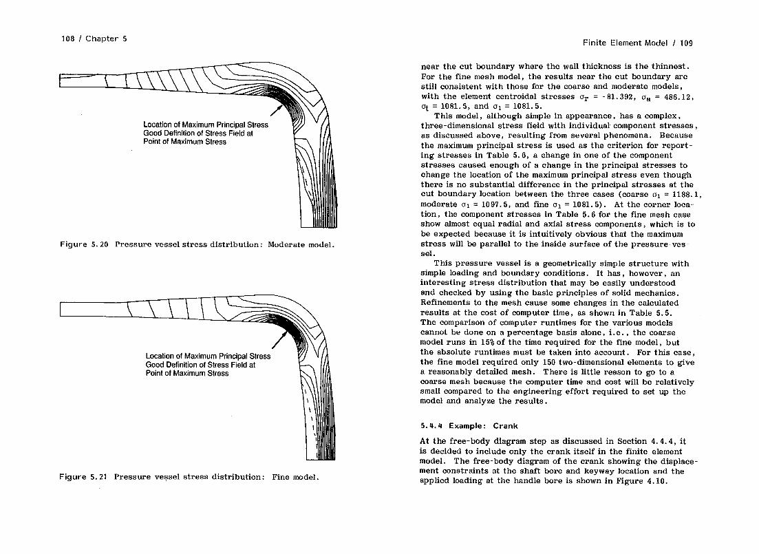
108 i Chapter 5 Finite Element Model / 109
Location of Maximum Principal Stress Good Definition of Stress Field at Point of Maximum Stress
Figure 5. 20 Pressure vessel stress distribution: Moderate model.
Location of Maximum Principal Stress Good Definition of Stress Field at Point of Maximum Stress
Figure 5.21 Pressure vessel stress distribution: Fine model.
near the cut boundary where the wall thickness is the thinnest. For the fine mesh model, the results near the cut boundary are still consistent with those for the coarse and moderate models, with the element centroidal stresses or = -81.392, a, = 486.12, at = 1081.5, and o1 = 1081.5.
This model, although simple in appearance, has a complex, three-dimensional stress field with individual component stresses, as discussed above, resulting from several phenomena. Because the maximum principal stress is used as the criterion for report- ing stresses in Table 5.6, a change in one of the component stresses caused enough of a change in the principal stresses to change the location of the maximum principal stress even though there is no substantial difference in the principal stresses at the cut boundary location between the three cases (coarse u1 = 1188.1, moderate u1 = 1097.5, and fine u1 = 1081.5). At the corner loca- tion, the component stresses in Table 5.6 for the fine mesh case show almost equal radial and axial stress components, which is to be expected because it is intuitively obvious that the maximum stress will be parallel to the inside surface of the pressure ves- sel.
This pressure vessel is a geometrically simple structure with simple loading and boundary conditions. It has, however, an interesting stress distribution that may be easily understood and checked by using the basic principles of solid mechanics. Refinements to the mesh cause some changes in the calculated results at the cost of computer time, as shown in Table 5.5. The comparison of computer runtimes for the various models cannot be done on a percentage basis alone, i.e. , the coarse model runs in 15% of the time required for the fine model, but the absolute runtimes must be taken into account. For this case, the fine model required only 150 two-dimensional elements to give a reasonably detailed mesh. There is little reason to go to a coarse mesh because the computer time and cost will be relatively small compared to the engineering effort required to set up the model and analyze the results.
5.4.4 Example : Crank
At the free-body diagram step as discussed in Section 4.4.4, it is decided to include only the crank itself in the finite element model. The free-body diagram of the crank showing the displace- ment constraints at the shaft bore and keyway location and the applied loading at the handle bore is shown in Figure 4.10.

110 / Chapter 5 Finite Element Model / 111
The crank is modeled with three-dimensional eight-node solid elements. The gridwork is shown in Figure 5.22. One layer of elements is used to model the flange connecting the shaft hub to the handle hub. One additional layer of elements is used to model the shaft hub and a third layer to model the handle hub. The model that is developed is suitable to give an overall representa- tion of the stresses in the crank without concentrating on any one area.
It may be anticipated that the highest stresses may occur at the corners of the keyway, and if that is the case, a finer grid may give a better resolution of the stress field and a better es- timate of the peak stress. A method for accomplishing this is refined mesh modeling, which is discussed in Chapter 9. With this technique, a second model of the keyway region is formed and displacements from the complete model corresponding to the outside boundaries of the refined model are transferred to the refined model. The difficulty in including a fine mesh near the keyway in the complete model is that it requires more total ele- ments in the model and several layers of transition elements to
Roller Constraints Along Nodes Representing Load Bearing Boundary of Keyway
3D Model - 224 Solid Elements 459 Nodes
No Attempt Made to Obtain Detailed Stresses at Keyway Corner
Figure 5.22 Crank model.
Pattern of Triangular Elements Used for Transition Reduction of 2:l for Each Transition Layer
Figure 5.23 Coarse to fine mesh transition.
reduce from the fine mesh to the coarse mesh, as shown in Figure 5.23.
A second area of potentially high stress that may be addressed with a refined mesh model is the welded interface of the shaft hub and the flange. This model does not attempt to represent the weld fillet and assumes homogeneous material. The model would be equally applicable to a crank made as a weldment or casting. Again, additional detail could be added to the interface at the expense of driving up the computer runtime. The computer

112 I Chapter 5
Table 5.7 Details and Computer Runtimes for Crank Model
Finite-Element Model / 113
Three-dimensional 224 Elements (three-dimensional, solid) 459 Nodes 1306 active DOF Times (see)
Element formulation 320.53 (1.431 sec/elem.) Wavefront solution 427.95 Stress solution 77.609 (0.346 sec/elem.) Element forces 5.821 Misc. 37.418
Total 924.38 set
Note: Computer runtimes are only valid for relative comparison between models and example cases.
Figure 5.24 Crank: Maximum principal stress distribution. runtime breakdown for this model is given in Table 5.7. This fairly uniform model is constructed without attempting to pre- suppose the exact location of maximum stress. In this way, the mode1 can give an estimate of the stress distributions and pro- vide data that may be used in subsequent refined model runs.
A plot of maximum principal stress results is shown in Figure 5.24. The results show two areas of high stress, the keyway and the interface of the shaft hub and flange. The maximum stresses for each location are given in Table 5.8.
5.4.5 Example: Gear Segment
Three different models are used to calculate the stresses in the gear segment with particular emphasis on the fillet area where fatigue cracks are known to develop, as discussed in Chapter 4, Section 4.2.5. The three models are the following.
1. Two-dimensional single tooth model Shown in Figure 5.25, this model uses roller constraints along its cut boundaries between the teeth and roller constraints along the base of the segment. The loading is applied directly to the tooth pressure surface based on the average force per length of the most heavily loaded section of length of the tooth. Figure 5.26 shows a pressure dis- tribution across three teeth in contact. The two-dimensional sin- gle tooth model represents a tooth as it is taking on its maximum loading.
Table 5.8 Stress Results of Crank Model
Maximum centroidal stress Maximum nodal stress
Keyway
*r at *a 01 or ot oa *I -371.38 785.90 66.8’7 1126.8 -538.41 814.92 30.00 1085.19
Hub-flange interface
llz. 9 78?62 % 01 3.96 1151.4 9%. 81 127 43
%A 01 -5.16 1014.06
or = radial stress at shaft bore, near keyway at = tangential stress at shaft bore, near keyway oa = axial stress at shaft bore, near keyway oi = maximum principal stress, near keyway ox = X direction stress, X axis is a line connection the two bores oy = Y direction stress, Y axis is in the plane of the flange, nor-
mal to the X axis 0 s = Z direction stress, Z axis is normal to the plane of the flange,
in the same direction as the axial direction above 01 = maximum principal stress

114 / Chapter 5 Finite Element Model / 115
Distributed Loading Resolved into Component Nodal Forces
60 2D Plane Strain Elements Fairly Uniform Mesh Density
Roller Constraints Along Cut Boundaries
Figure 5.25 Two-dimensional single gear tooth model.
2. Two-dimensional three-tooth segment model Shown in Fig- ure 5.27, this model is simply the single tooth model repeated three times. Loadings are applied to the profile in the same man- ner as for the single tooth model. Roller displacement constraints are used along the cut boundaries and the bottom of the segment. Loadings are applied to all three teeth in a manner that repre- sents the instant at which the maximum loading is on the center tooth.
Note: Difference in Loading Between Teeth (Both Location and Magnitude) due to Angular Position of Teeth Relation to Mating Gear Teeth
Figure 5.26 Pressure distribution across three teeth.
Distributed Loading Resolved into Component Nodal Forces
ktler Constraints Along Cut Boundaries Segment Model Will Allow for Compressive Stress Effects toBe Calculated 180 20 Plane Strain Elements Same Mesh Pattern as Single Tooth Model But Repeated to Form Segment
Figure 5.27 Two-dimensional three-tooth segment model.
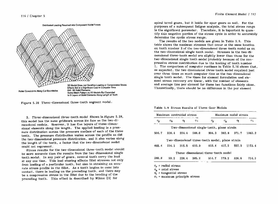
116 I Chapter 5 Finite Element Model / 117
Distributed Loading Resolved into Component Nodal Forces
crifice Loading or Compressive ant Cost in Computer Time
Roller Constraints Along Cut Boundaries 840 3D Solid Elements Same Mesh Pattern as 2D Models But Expanded to 5 Layers of Solid Elements Along Length of Tooth
I Stress
spiral bevel gears, but it holds for spur gears as well. For the purposes of a subsequent fatigue analysis, the total stress range is the significant parameter. Therefore, it is important to quan- tify this negative portion of the stress cycle in order to accurately determine the cyclic stress range.
The results of the two models are given in Table 5.9. This table shows the maximum stresses that occur at the same location on tooth number 2 of the two-dimensional three-tooth model ‘as on the two-dimensional single tooth model. Stresses in the two-di- mensional three-tooth model are slightly lower than those for the two-dimensional single tooth model probably because of the com- pressive stress contribution due to the loading of tooth number 1. The comparison of computer runtimes in Table 5.10 shows that, as expected, the two-dimensional three-tooth model required just over three times as much computer time as the two-dimensional single tooth model. The times for element formulation and ele- ment stress recovery are linear , with the number of elements and average time per element for these two functions fairly close. Theoretically, there should be no difference in the per element
Figure 5.28 Three-dimensional three-tooth segment model.
Table 5.9 Stress Results of Three Gear Models
3. Three-dimensional three-tooth model Shown in Figure 5.28, this model has the same gridwork across its face as the two-di- mensional models. However, it has five layers of three-dimen- sional elements along the length. The applied loading is a pres- sure distribution across the pressure surface of each of the three teeth. The pressure distribution varies across the profile as did the two-dimensional pressure distribution, and it also varies along the length of the teeth, a factor that the two-dimensional model could not represent.
Stress results for the two-dimensional three-tooth model should be more accurate than the results from the two-dimensional single tooth model. In any pair of gears, several teeth carry the load at any one time. This load sharing affects fillet stresses not only from loading of a particular tooth, but also in obtaining an accu- rate stress profile in the fillet. As a tooth begins to come into contact, there is loading on the preceding tooth, and there may be a compressive stress in the fillet due to the bending of the preceding tooth. This effect is described by Wilcox [ 31 for
Maximum centroidal stress Maximum nodal stress
or oa at 01 Or Oa ot 01
Two-dimensional single-tooth, plane strain
506.7 228.4 254.4 588.0 904.3 382.8 371.7 1063.2
Two-dimensional three-tooth model, plane strain
465.4 234.3 315.5 632.9 833.4 417.2 557.2 1173.4
Three-dimensional three-tooth model
280.8 99.2 228.4 385.2 514.7 179.2 326.6 714.3
or = radial stress Oa = axial stress at = tangential stress o1 = maximum principle stress

118 1 Chapter 5 Finite Element Model / 119
Table 5.10 Details and Computer Runtimes for Gear Models
Two-dimensional single tooth 60 Elements (two-dimensional, plane strain) 79 Nodes 135 active DOF Times (see)
Element formulation Wavefront solution Stress solution Element forces Misc.
13.14 (0.219 sec/elem.) 3.767 3.955 (0.066 seclelem.) 0.445
13.03
Total 34.337 set
Two-dimensional three-tooth segment 168 Elements (two-dimensional, plane strain) 211 Nodes 421 active DOF Times (see)
Element formulation 39.03 (0.232 sec/elem.) Wavefront solution 21.47 Stress solution 17.05 (0.101 sec/elem.) Element forces 12.46 Misc. 30.83
Total 120.83 set
Three-dimensional three-tooth segment 840 Elements (three-dimensional, solid) 1270 Nodes 3808 active DOF Times (set)
Element formulation 1198.09 (1.426 sec/elflm.) Wavefront solution 3332.49 Stress solution 250.748 (0.299 sec/elem.) Element forces 297.542 Misc. 301.192
time for element formulation and stress recovery. A technique for minimizing computer time for repetitive structures such as the gear teeth is substructuring, which is discussed in more de- tail in Chapter 10.
Plots of maximum principal stresses are shown in Figure 5.29 for the two-dimensional single tooth model and in Figure 5.30 for the two-dimensional three-tooth model.
Location of Maximum Principal Stress Maximum Tensile Bending Stress Occurs in Fillet as Anticipated
Total 5380.07 set
Note: Computer runtimes are only valid for relative comparison between models and example cases. Figure 5.29 Two-dimensional single tooth model stress distribu-
tion .

120 / Chapter 5 Finite Element Model / 121
Location of Maximum Principal Stress Note: Compressive Stress in Fillet
/
Sharp Stress Gradient from Compressive Stress to Tensile Stress
Figure 5.30 Two-dimensional three-tooth model stress distribu- tion .
30 Model Shows Elliptical Loading Areas on Pressure Faces
In order to fully utilize the two-dimensional three-tooth model, there should be a series of static runs with the loading changed between and over the teeth to simulate the teeth, and especially tooth number 2, as they roll through contact. The results of this series of runs, when assembled, provide a pseudodynamic stress time history for a tooth. Required input to such a series of runs would be a description of the force distribution on the contacting teeth as a function of angular position (time). This drawback could be eliminated by expanding the two-dimensional model to include three teeth from the driving gear as well as the driven gear and using gap elements to represent the contact be- tween the teeth.
The three-dimensional three-tooth model uses the same element density per plane as the two-dimensional three-tooth model. The three-dimensional model uses five layers of elements along the length of the teeth as shown in Figure 5.28. A stress contour plot for the three-dimensional model is shown in Figure 5.31.
The three-dimensional model has three basic advantages over the two-dimensional models : (1) the three-dimensional models calculate the full three-dimensional stress field, the two-dimen- sional models cannot calculate an axial stress or associated shear
Location of Maximum Principal Stress Lengthwise Variation in Stress Follows Variation in Loading en Any Given Plane Pattern of Stress Follows 2D Pattern
Figure 5.31 Three-dimensional three-tooth model stress distribu- tion .
stresses; (2) the three-dimensional model can account for a vari- ation in contact pressure along the length of the tooth; (3) the three-dimensional model, if used together with a gear segment model of the mating gear, can include lengthwise %rowning” of the teeth to accurately evaluate its effect on contact pressure. Lengthwise crowning is used to localize the contact pattern into a well-defined ellipse that is less susceptible to deflections of the gears and their bearings. Without crowning, there will be full contact along the length of the teeth under perfect alignment conditions, but highly localized line contact under less than per- fect conditions.
A comparison of stresses between the two-dimensional three- tooth model and the three-dimensional three-tooth model shows

122 I Chapter 5 Finite Element Model I 123
that the location of the maximum stress occurs at approximately the same location in the fillet. The magnitude of the stresses in the three component directions is about of the same magnitude. There are two reasons for the differences in stress: (1) The two-dimensional model uses a plane strain calculation to obtain the axial stresses, whereas the three-dimensional model calcu- lates these stresses directly, and (2) the loading of the three- dimensional model is distributed over the length of the gear tooth rather than applying an average force per length in the two-di- mensional model.
The more sophisticated three-dimensional analysis is not with- out its price. The three-dimensional model with its 840 solid elements and 3808 active degrees of freedom required 44.5 times as much computer time as the two-dimensional three-tooth model with only 168 two-dimensional elements and 421 active degrees of freedom. The decision as to whether or not to use a three- dimensional model is obviously not made without a good under- standing of the requirements of the analysis and the operating conditions of the gear set.
5.4.6 Example: Turbine Blade
A three-dimensional model using eight-node solid elements is de- veloped from the turbine blade and shown in Figure 5.32. A por- tion of the cover is included in the model to properly apply cen- trifugal loading to the tenon, as described in the discussion of the free-body diagram. A segment of the rotor around the blade root attachment is also included in the model, as shown in the free-body diagram (Figure 4.13).
Attachment between the tenon and cover is made by coupling all three degrees of freedom at the appropriate nodes. In the blade root-rotor attachment, the nodes along the six contact sur- faces are coupled. No attempt is made to use gap elements to represent the interface as they require a nonlinear, iterative so- lution and would significantly increase the computer time.
A total of 774 elements is used in the model. This allowed for a reasonable representation of the airfoil section with two elements across the thickness, eight elements across the chord, and 18-ele- ment layers along the length (Figure 5.33). Accurate geometric modeling of the airfoil geometry is more important in the calcula- tion of natural frequencies and dynamic response than in the cal- culation of static stress.
Full 3D Model Required Segment of Rotor Included for Proper Calculation of Stress in Blade Root Area
Figure 5.32 Turbine blade model.
Six elements are used to represent the tenon and eight ele- ments are used in the cover (Figure 5.34). This is sufficient to apply the centrifugal loading to the airfoil tip, but not really adequate to model the stresses at the tenon-cover interface or at the fillet between the tenon and airfoil tip. Although the blades are connected by the cover into groups of three, a sim- plifying assumption is made that under static loading, all three blades in the group will see approximately the same stress. Therefore, a single blade with one cover segment is used with constraints on the sides of the cover segment to prevent rota- tion .
A total of 335 elements are used in the combined blade and rotor root attachment area. The details of the blade root portion

124 / Chapter 5 Finite Element Model I 125
Rotor Segment Removed to Show Model of Blade Root
Figure 5.33 Turbine blade model without rotor segment.
of the model are shown in Figure 5.35 and the rotor slot model is shown in Figure 5.36. The nodes in the blade root portion of the model are separate .from the nodes of the rotor slot portion. The contact between the blade root and rotor slot is modeled by coup- ling the coincident pairs of nodes on the contact surfaces. The root cross section is capable of giving a reasonable approximation of the highly localized stresses in that area. A refined two-di- mensional model may be used to give a better resolution of the peak stresses, as discussed in Chapter 9.
Computer runtimes for the three-dimensional model are given in Table 5.11. Stress results for the various components of the model are given in Table 5.12. Plots of maximum principal stress
Coarse Model of Cover-Tenon Interface Localized Stresses Will Not Be Accurate
One Pitch of Continuous Cover Band
I/ Included in Model Attached by Tenon
Figure 5.34 Turbine blade model: Cover details.
distributions are given in Figures 5.37 for the airfoil section and 5.38 for the root section.
5.5 SUMMARY
Developing the most cost-effective model requires the combination of knowledge of finite element principles, behavior of the struc- ture to be analyzed, and engineering experience and judgment. The process that some engineers consider to be an art can, how- ever, be made into more of a science by taking a step-by-step approach and isolating the critical gridwork layout step. Prob- ably, the most critical item in determing the number and place- ment of elements within the gridwork is understanding of the be- havior of the selected element. The following chapter gives data and some discussion into the properties of some common elements.

Note: Complex Transition Between Airfoil and Platform Sections Virtually Impossible to Avoid. Distorted Elements in Transition Stresses in These Elements Should Be Ignored
Airfoil
Platform
Figure 5.35 Turbine blade model: Blade root details.
Finite Element Model / 127
Coupled Nodes Between Load Bearing Surfaces of Rotor Segment and Blade Root
Rotor Disk
Roller Constraints on Cut Boundaries of Rotor Segment
Figure 5.36 Turbine blade model: Rotor slot details.
Table 5.17 Details and Computer Runtimes for Turbine Blade Model
‘774 Elements (three-dimensional, solid) 1184 Nodes 3302 active DOF Times (set)
Element formulation 1106.82 (1.430 sec/elem.) Wavefront solution 3132.66 Stress solution 229.878 (0.297 sec/elem.) Element forces 273.302 Misc. 288.652
Total 5031.31 set
Note : Computer runtimes are only valid for relative comparison between models and example cases.

Table 5.12 Stress Results of Turbine Blade Model Finite Element Model / 129
Maximum centroidal stress
Cover 6317.2 16171.0 7656.1 30474.0
Tenon 37560.0 2869.6 -6300.2 40353.0
Airfoil 59789.0 2177.9 1584.4 61665.0
Root attachment 95164.0 33315.0 43192.0 96797.0
a, = radial stress. 5 a = axial stress. at = tangential stress. cl = maximum principal stress.
Note: Location of Maximum Principal Stress in Upper Hook Fillet
Figure 5.38 Turbine blade root principal stress distribution.
REFERENCES
1. Seeley , F. B. and J. 0. Smith, Advanced Mechanics of Ma- terials, 2nd ed. , Wiley, New York, 1932, pp. 304-306.
2. Timoshenko, S. , Strength of Materials - Part II, 3rd ed., Van Nostrand, New York, pp. 205-214.
3. Wilcox, L. E., “An Exact Analytical Method for Calculating Stresses in Bevel and Hypoid Gear Teeth,” Proceedings of International Symposium on Gearing and Power Transmission, Tokyo, Japan, 1981.
Maximum Principal Stresses Location of Maximum Principal Stress in Root Notch
Figure 5.37 Turbine blade model stress distribution.

6
DEBUGGING FINITE ELEMENT MODELS
A large proportion of the total time in generating a finite element model is spent in debugging the model. Prior to the use of in- teractive mesh generation programs, the time spent in model de- bugging, correction, and input data editing (either card decks or batch input files) could exceed the time for actual data input by a factor of 2 or 3. The use of interactive graphic mesh gen- eration software has had its greatest impact on cutting model de- bugging time by allowing the user to view each part of the model as it is input and make corrections immediately, when necessary. Even with the older batch-type input, models could be developed with a minimum number of input statements; however, there was always a tendency to build an entire model before submitting a check run to look for errors. Error location was difficult because a plot of the entire model may reveal several problems that would be hard to pinpoint.
A typical finite element model can be divided into four areas:
Geometry. Material properties.
131

132 I Chapter 6
Table 6.1 Common Symptoms and Their Possible Causes
Excessive deflection, but anticipated stress
Excessive deflection and excessive stress
Internal discontinuity in stress and deflection
Discontinuity along bound- ary
Higher or lower natural frequencies than antici- pated
Static deflections, 0. K . Static deflections, not 0 .K .
Internal gap opening up in model under load, stress discontinuity
Young’s modulus too low, miss- ing nodal constraints
Applied force too high, nodal coordinates incorrect, force applied at wrong nodes
Force applied at wrong node, missing or double internal ele- ment
Missing nodal constraint, force applied at wrong node
Density incorrect Young’s modulus incorrect
Improper nodal coupling
Applied forces. Displacement constraints.
Some of the more common problems in these areas are given in Table 6.1 and discussed in the following sections.
6.1 GEOMETRY
Geometry problems can be classified as ob@ous (element distor- tion) and not so obvious (unconnected or missing elements, slight inaccuracies in dimensions). The obvious problems stem from the nodal coordinates and/or element descriptions that result in badly distorted elements in an element plot.
When data are input interactively, it is recommended that plots be made frequently, i.e. , as each set of nodes or elements are either input or generated (Figures 6.1 and 6.2).
Note: Difficulty in Determining Exact Problem Element Connected to Wrong Node or Node out of Position
9141g2h .-
37 87 99
WA 50 26
88 -- 100 39
29
19
81 YY
32 82
21
94 33
83 95 71
22 34
72 84
11 23
61 73 85
12 24
62 74 1 13
63 75 51
2 14 52 64
3 53 65
4 54
96 35
86 25
76 15
66 5
36 98
77 89
16 28 78
17 67 79
6 18 68
‘I
40 90
55 30 80
56 L
57 79 8 20
kfl3D Nodal Pattern Still Difficult 58 70 - B Determine Which Node Is out of Position 9
59 10
60
Figure 6.1 Simple note and element pattern with single nodal error.

134 I Chapter 6 Debugging Finite Element Models I 135
41
31
21
11
1
42
32
22
12
2
43
33
23
13
3
44
34
24
14
4
Single Plane of Nodes - Node 27 is out of Position
45
35
25
15
5
46
36
26
16
6
47
37 48
??a
17 28
7 18
8
49
39
29
19
9
50
40
30
20
10
2D Node Pattern for X,Y Plane Does not Reveal Problem Because Node 27 Is out of Plane with the Incorrect Z Coordinate
41 42 43 44 45 46 47 48 49 50
31 32 33 34 35 36 37 38 39 40
21 22 23 24 25 26 27 28 29 30
11 12 13 14 15 16 17 18 19 20
1 2 3 4 5 6 7 8 9 10
Figure 6.2 Three-dimensional nodal pattern plot slowing error in nodal location.
Nodes are typically input first and plots of nodal patterns should be made at each major step in the generation process. Once the user is satisfied that the nodal pattern is correct, the element connectivity may be entered. Then if elements appear to be improper, the user knows that it is an error in the element numbering. If no plots are made until the elements are entered, the user does not know whether the error is in the nodes or ele- ments and the user must “back track” to find the error.
When a complex model is being generated, it is advisable to enter nodes and elements in sections rather than try to enter all the nodes and, then, all the elements. The rule of thumb should be not to enter more data at a time than can be verified by one or two plots. It is much easier to fix problems as they occur than to let an error slip through that may not be noticed.
Not so obvious element geometry problems are missing or over- lapping elements : coupled nodes and small errors in nodal co- ordinates. Missing elements can most often be discovered by using a “shrink” option for element plotting as shown in Figure 6.3.
One or more missing internal elements may be difficult to pick up if all adjacent elements are present. By the same token, it is possible to define double elements in the same space attached to the same nodes. The finite-element program will accept this and the result will be double stiffness, or a hard spot, in the model that will be difficult to determine without a thorough ex- amination of the results. The dangerous aspect of missing or double elements is that they probably do not affect the results enough to be obvious, but could lead to inaccuracies in the range of 5-10s.
When complex models are developed, they are sometimes gen- erated in sections with coincident, but uniquely defined nodes along their common boundary. The intention is to couple these coincident nodes; however, this must be checked by a printout of a check run because an element plot typically would not re- veal a problem because the nodes are coincident. If graphics software is available that can highlight free surfaces, this may reveal any internal gaps in the model.
Another area that can lead to inaccuracies is nodal coordinate errors, which cannot be picked up by a visual inspection. An error of 10% on a dimension of a model may not be obvious in an element plot, but will be significant in the final results. When constructing a model, it is advisable to compare the model co- ordinates against the structure’s blueprint. This involves

Shrink Option Makes It Obvious That There Is a Missing Element
Without Shrink Option It Cannot Be Determined That There Is a Missing Element
Figure 6.3 Plate with missing element shown using shrink option.
Debugging Finite Element Models / 137
extracting nodal coordinates of key points on the model and making the appropriate subtractions to compare to the linear dimensions of the blueprint.
6.2 MATERIAL PROPERTIES
Data input for material properties is minimal: Young’s modulus and Poisson’s ratio are always required. For dynamic models, mass density is also required. For thermal models, specific heat, conductivity, and boundary data such as film coefficients or ra- diation view factors may also be required. Material properties must be checked by having the program echo back the input data either to a terminal or in a printout. The user should never assume that he entered the data correctly even if it seems simple. This print-back takes only a few seconds, but must be checked carefully to avoid embarrassing mistakes later in the analysis.
The two most common mistakes are
1. Young’s modulus is incorrect by a power of 10. 2. Inconsistent units are assumed for material density. Be-
cause the finite element method is nondimensional, the user must insure that the units assumed for density are consistent with the units used. for stiffness, time, force, and acceleration in a dynamic analysis.
When more than one material is used in a model, some element plot routines can indicate the different materials with different colors for checking.
6.3 APPLIED FORCES
Forces must be applied at the nodes in (1) the proper magnitude, (2) the proper location, and (3) the proper direction. Forces may be checked either from the print-back or from a node or ele- ment plot with the appropriate force display option selected.
In checking to see if the forces are applied at the correct lo- cation, both the node number and the location of the node must be checked, i.e., the node number may be correct but if the no- dal coordinates are not correct, the force will not be applied at the correct location. Element or node plots ‘with a force bound- ary condition option selected will show the locations and direc- tions of the applied forces. The actual force magnitude must

138 I Chapter 6 Debugging Finite Element Models / 139
be checked from a print-back, either from a terminal or print- out.
A nodal map, i.e., a plot of the node locations, is a great help in assigning and checking nodal force loadings.
As in the case of material properties, care must be taken to insure that the units selected are consistent with the nodal co- ordinates and material properties. One parameter that can cause problems is rotational speed when centrifugal force is applied. To be consistent with the equation, units must appear in radians per second (rad lsec) :
F=mro*
where
F = force (lbf)
m = mass in1b/fsec2 .
r* = length, radius (in.) w = radlsec
6.4 DISPLACEMENT CONSTRAINTS
Checking of displacement constraints is similar to checking ap- plied forces. Generally, nodes are constrained with a displace- ment of 0, which leaves only proper location and direction. Here again, a node map and the use of a node or element plot with the boundary condition option selected are very useful.
Two common problems with displacement boundary conditions’ are (1) missing constrained nodes and (2) an overconstrained boundary. When a series of nodes is representing a uniformly constrained boundary, a missing nodal constraint can lead to a local stress discontinuity and overall higher displacements. When specifying constraints along a symmetry boundary, care must be taken not to overconstrain the boundary by specifying more de- grees of freedom per node than are appropriate.
6.5 SUMMARY
is the total time from the definition of the problem to the $oint of obtaining useful results. A good checklist is invaluable in work- ing out finite element model problems. No piece of data should be taken casually or assumed to be correct. Experienced users check even the most simple input data when a problem is encoun- tered . More often than not, the problem is something embar- rassingly simple.
The use of interactive computer graphics has made possibly its strongest contribution to finite-element analysis productivity in assisting the user to debug models. The efficiency of an analy- sis must be measured in terms of net time for the analysis, which

7
ELEMENT PERFORMANCE
In forming a finite element model, probably the most critical de- cision is the type of elements to be used. The various types of elements each have a particular geometry and characteristics that allow them to model certain “theoretical” shapes with nearly per- fect accuracy. For example, plate elements will model a simple plate in tension or bending with a minimal number of elements, and a single element will suffice if the structure is simple enough.
Actual structures are hardly ever so simple that they can be perfectly represented by only a few elements (if they were, there would be no need for the finite element method). In real cases, the engineer must make his decision on which elements to use to model his structure. Following that, he needs to determine the absolute and relative element densities to use to achieve the de- sired accuracy with an acceptable computer runtime.
Chapter 2 discussed the various types of elements and their mathematical formulations. The main element categories are
141

142 I Chapter 7
Two-dimensional, plane stress /plane strain / axisymmetric Three-dimensional, solid Plate and beam
Within each general category there are parameters that differen- tiate the element’s behavior. For two- and three-dimensional solid elements, the main differences are the order of integration, method of formulation of the stiffness matrix, method of resolu- tion of mass, and number of integration points used for Gaussian quadrature integration. The most common element types, clas- sified according to their geometry, are given in Table 7.1 and shown in Figures 7.1-7.5.
Table 7.1 Classes of Element Geometry Types
I Two-dimensional plane stress, plane strain, axisymmetric Quadrilateral or triangle 2 DOF per node Ref. : Chapter 2, Section 2.5-2.6 Figure 7.1
II Three-dimensional solid Hexahedron (brick), wedge, or tetrahedron 3 DOF per node Ref. : Chapter 2, Section 2.8 Figure 7.2
III Plate Quadrilateral or triangle 6 DOF per node Ref. : Chapter 2, Section 2.8 Figure 7.3
IV Beam No shape, two nodes representing end points; cross-sec-
tional properties specified directly 6 DOF per node Ref. : Chapter 2, Section 2.8 Figure 7.4
V. Specialty elements Point mass Spring Damper Gap Figure 7.5
2D Plane Stress and Plane Strain
n
Element Performance I 143
i ,-
dY
1 Ll LINEAR (constant strain) QUADRATIC (linear strain)
I I I I I AXISYMMETRIC LINEAR TRIANGLE
Figure 7.1 Two-dimensional elements; three or four nodes; 2 DOF per node.
3D Solid
3 D SOLID PRISM &NODE 3D SOLID WEDGE 6-NODE
Figure 7.2 Three-dimensional solid elements: 3 DOF per node.

144 I Chapter 7 Element Performance / 145
Plate and Beam
PLATE 4-NODE
Figure 7.3 Plate elements: three or four nodes; 6 DOF per node.
The accuracy of any finite element model is strongly dependent on the type of elements used in the model, as well as the number of elements, their relative distribution, the type of loading, and the amount of element distortion. Table 7.2 lists the main parame- ters that affect element accuracy. There is no simply defined re- lationship between the parameters listed in Table 7.2, and it would be wrong to assume that net accuracy (or error) would simply be a linear combination of some value assigned to each of the parame- ters. In addition to individual element accuracy, the net accuracy of a model is a function of how well the selected elements match the structural geometry, e.g. , straight-sided elements approxi- mating a curved boundary.
BEAM P-NODE
Figure 7.4 Beam elements: 6 DOF per node.
Spring ConnectsTwo Nodes with aSingle DOF Stiffness More Than One Spring May Be Used to Connect Nodes with Multiple DOF
Gap High Stiffness when Closed (1 Ox Stiffness of Surrounding Elements) Zero Stiffness when Open Allows for Sliding and Incorporates Friction Effects
Lumped Mass May Be Applied to One or More DOF at a Node
Figure 7.5 Specialty elements.

146 I Chapter 7 Element Performance / 147
Table 7.2 Parameters Affecting Element Behavior and Accuracy
I Element type 1. Two-dimensional, plane stress/plane strain/axisymmetric 2. Three-dimensional solid 3. Plate 4. Beam
II Integration order 1. Linear 2. Quadratic 3. Linear with added displacement shapes
III Method of formulation 1. Assembly of triangles or tetrahedra 2. Isoparametric
IV Number of integration points 1. Full 2. Reduced 3. Selectively reduced
V Degree of distortion 1. Aspect ratio 2. Parallelogram angle 3. Trapezoid angle
VI Element Density 1. Number of elements across width 2. Number of elements along length 3. Number of elements across thickness
VII Type of loading 1. Tension 2. Bending, in plane 3. Bending, out of plane 4. Torsion
7.1 ELEMENT INTEGRATION ORDER
For two-dimensional plane stress/plane strain/axisymmetric and three-dimensional solid elements, the feature that subdivides each of these element classes is the element integration order. The
dy 2 DOF per Node UX, UY
First-Order - Constant Strain, Linear Variation in Displacement; Constant orAverageStrainWithinElement; Isoparametric
Figure 7.6 Linear displacement element.
basic mathematics of order of integration are explained in Chap- ter 2, Section 2.9. The order of integration is divided here into three categories : linear displacement (LD) (Figure 7.6)) linear displacement with added displacement shapes (LDADS) (Figure 7.7)) and quadratic displacement (QD) (Figure 7.8). When in- specting a model, both of the two linear displacement element
1 II 2 Midside Flexural DOF
First-Order with Additional Displacements Psuedo Higher-Order Additional Shapes Allow for Flexing of Element Sides Subparametric
Figure 7.7 Linear displacement with added displacement shapes element.

148 I Chapter 7 Element Performance / 149
2 DOF per Node : Corner Nodes and Mid-Side Nodes
Second-Order; Mid - Side Nodes
Quadratic Variation in Displacement Linear Variation in Strain, lsoparametric More Efficient, Higher accuracy over First Order Can Model Curved Boundary Directly Not asCost Effective as First-Order with Added Displacement
Figure 7.8 Quadratic displacement element.
categories, LD and LDADS , can be recognized as having nodes only at their vertices. The quadratic elements can be recognized by their midside nodes. It is important to note that both of the linear displacement elements appear identical from the surface; however, it will be shown that they have significantly different behavior. This same caveat holds true for other element types in which elements with identical outward appearance will show significantly different results, and the user must be careful to look below the surface to investigate the specific properties of any element before using or interpreting results.
The linear displacement with added displacement shapes ele- ments almost always show superior performance compared with the unmodified linear displacement elements. The LDADS ele- ments have two drawbacks, however : 1) They may fail the “patch test ,‘I meaning that the continuity of displacement is not guaranteed along element boundaries between the nodes as in the case of the LD elements. 2) There is no equivalent tri- angular, wedge, or tetrahedron element, so that when these elements are mixed in a model with LDADS elements, there is an incompatibility between them, and the triangular, wedge, and tetrahedra elements are “overstiff. I’ This results in a lo- cally “hard spot” in the model.
The differences between the three element categories are sum- marized in Table 7.3, along with appropriate figure numbers and references.
7.2 ELEMENT PERFORMANCE TESTS
Due to the number of parameters involved in element perform- ance as outlined in Table 7.2, the only practical way of providing information on the relative and absolute performance of the vari- ous element types is by a series of example problems run with various combinations of element types. This sort of test pro- vides an empirical performance standard. A selection of the most commonly used element types are given in Table 7.4, along with their designation to be used in the subsequent test cases.
A set of test cases has been published by MacNeal and Harder [ 11 as a proposed set of standards to test finite element accuracy. This set of problems represents a good set of benchmark prob- lems in that they begin to approach “real life” problems, but still have exact solutions available for absolute comparison. One dif- ficulty with using very simple shapes such as uniform cylinders, plates, and beams is that they do not allow for the inclusion of the effects of element distortion or geometric discontinuities. The very simplistic comparison problems often show good re- sults with only a few elements, thereby prohibiting any evalua- tion of element convergence. The following sections give results for the generic element types: two-dimensional plane stress / plane strain/axisymmetric, three-dimensional solid, plate, and beam. These are listed in Table 7.4 for problems taken from the MacNeal-Harder set and others.
The value of a set of benchmark problems is not only that it provides useful information on element performance, but it also provides a good reference against which to test specific finite element codes. One way to get a projection of the accuracy of a particular finite element model would be to select a similar benchmark problem for which an exact solution is available, and to run that problem with the specific finite element code and elements that will be used ‘for the actual model and vary the ele- ment density to test its influence on accuracy.
Virtually all commercial finite element codes are undergoing continual development and upgrades, with new releases being is- sued on a regular basis. Any set of actual element performance numbers, even those generated with an accepted set of bench- mark problems such as the MacNeal-Harder set, may be obsolete
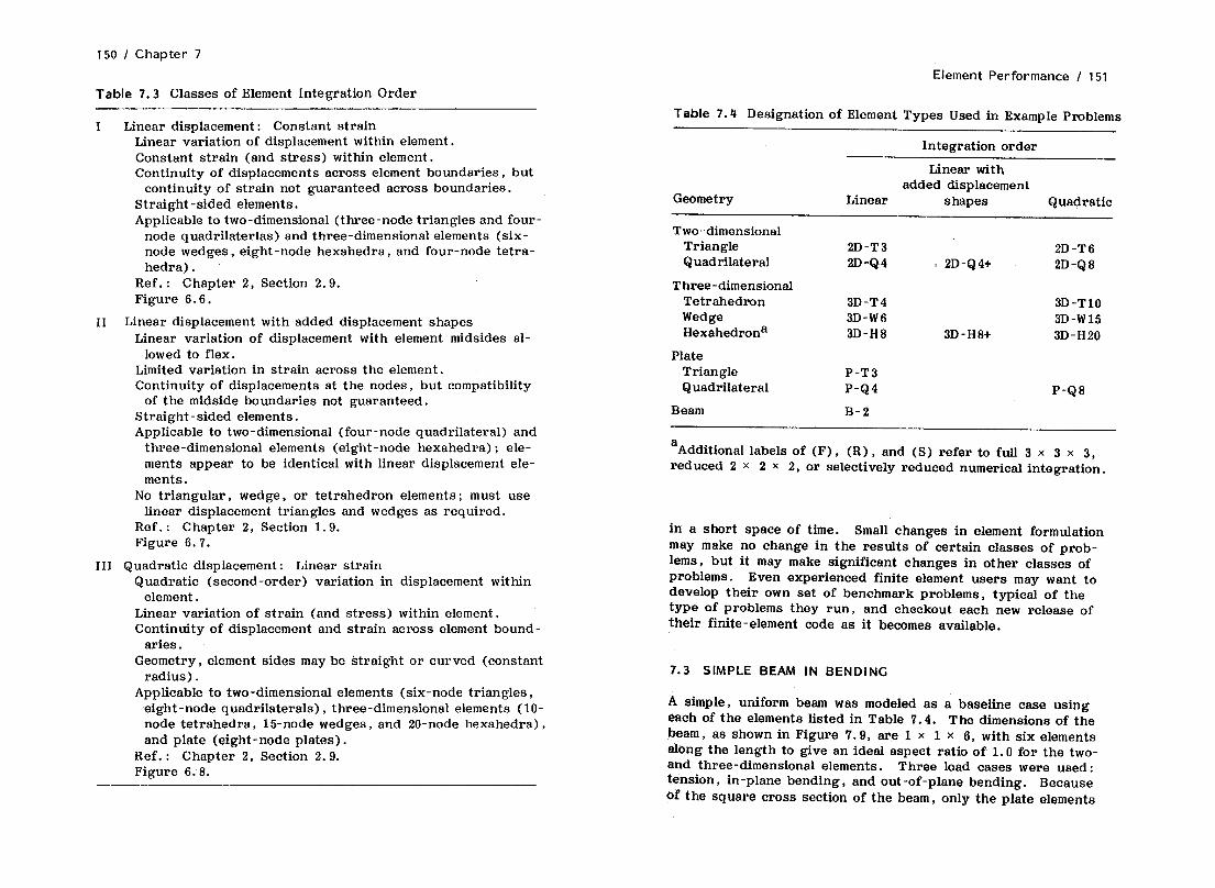
150 I Chapter 7
Table 7.3 Classes of Element Integration Order Element Performance / 151
I Linear displacement : Constant strain Linear variation of displacement within element. Constant strain (and stress) within element. Continuity of displacements across element boundaries, but
continuity of strain not guaranteed across boundaries. Straight-sided elements. Applicable to two-dimensional (three-node triangles and four-
node quadrilaterlas) and three-dimensional elements (six- node wedges, eight-node hexahedra, and four-node tetra- hedra) .
Ref. : Chapter 2, Section 2.9. Figure 6.6.
II Linear displacement with added displacement shapes Linear variation of displacement with element midsides al-
lowed to flex. Limited variation in strain across the element. Continuity of displacements at the nodes, but compatibility
of the midside boundaries not guaranteed. Straight-sided elements. Applicable to two-dimensional (four-node quadrilateral) and
three-dimensional elements (eight-node hexahedra) ; ele- ments appear to be identical with linear displacement ele- ments.
No triangular, wedge, or tetrahedron elements; must use linear displacement triangles and wedges as required.
Ref. : Chapter 2, Section 1.9. Figure 6.7.
III Quadratic displacement : Linear strain Quadratic (second-order) variation in displacement within
element. Linear variation of strain (and stress) within element. Continuity of displacement and strain across element bound-
aries . Geometry, element sides may be straight or curved (constant
radius). Applicable to two-dimensional elements (six-node triangles,
eight-node quadrilaterals), three-dimensional elements (lo- node tetrahedra, 15-node wedges, and 20-node hexahedra) , and plate (eight-node plates).
Ref. : Chapter 2, Section 2.9. Figure 6.8.
Table 7.4 Designation of Element Types Used in Example Problems
Integration order
Linear with added displacement
Geometry Linear shapes Quadratic
Two-dimensional Triangle 2D-T3 2D-T6 Quadrilateral 2D-Q4 I 2D-Q4+ 2D-Q8
Three-dimensional Tetrahedron 3D-T4 3D-TlO Wedge 3D-W6 3D-W 15 Hexahedrona 3D-H8 3D-H8+ 3D-H20
Plate Triangle P-T3 Quadrilateral P-Q4 P-Q8
Beam B-2
‘Additional labels of (F), (R) , and (S) refer to full 3 x 3 x 3, reduced 2 x 2 x 2, or selectively reduced numerical integration.
in a short space of time. Small changes in element formulation may make no change in the results of certain classes of prob- lems, but it may make significant changes in other classes of problems. Even experienced finite element users may want to develop their own set of benchmark problems, typical of the type of problems they run, and checkout each new release of their finite-element code as it becomes available.
7.3 SIMPLE BEAM IN BENDING
A simple, uniform beam was modeled as a baseline case using each of the elements listed in Table 7.4. The dimensions of the beam, as shown in Figure 7.9, are 1 x 1 x 6, with six elements along the length to give an ideal aspect ratio of 1.0 for the two- and three-dimensional elements. Three load cases were used: tension, in-plane bending, and out -of-plane bending. Because Of the square cross section of the beam, only the plate elements

152 I Chapter 7 Element Performance / 153
Table 7.5 Simple Cantilever Beam in Bending 1 x 1 x 6, Normalized Tip Displacements for Various Element Types Perfect Cubic-Shaped Elements
Moment Loading at Free End
Figure 7.9 Uniform beam 1 x 1 x 6.
used both of the bending load cases. For the other elements, bending in the two directions gives identical results. The in- tention of this case is to provide a baseline for evaluating the elements under the most simple and ideal conditions possible. Displacement results of the calculations are given in Table ‘7.5. Results are presented in the form of normalized displacements, i.e., calculated displacements divided by theoretical displace- ments. Equally important are computer runtimes for the vari- ous elements shown in Table ‘7.6.
These results show that the performance, in bending, of the LDADS elements [ 2D-Q4+ 3D-H8+(R)] were far superior to that of the LD elements [2D-Q4 3D-H8(R)], both in terms of absolute accuracy and also the ratio of accuracy to runtime. In tension, there is no significant difference in results. This is because the added displacement shapes in the LDADS elements only af- fect element flexure. In simple tension, the sides of the element remain straight and, therefore, the added displacement shapes have no affect on element performance. Because of the perfect geometry, one would not expect to see any patch-test-type, dis- placement discontinuity problems.
The LDADS elements showed almost equal accuracy, in bend- ing, to the QD elements (2D-Q8 3D-H20) with a significantly
Number of Element type elements Tension Bending Y Bending 2
2D-Q4+ 6 0.996 1.011
2D-Q4 6 0.995 0.688 2D-T3 12 0.990 0.242
PD-Q8 6 1.148 1.005
3D-H8+(R) 6 0.988 0.994 0.994
3D-H8+(F) 6 0.988 0.994 0.994
3D-H8 6 0.985 0.652 0.652
3D-H20 6 1.250 0.988 0.988
3D-W6 12 0.969 0.218 0.724
P-Q4
P-Q8
B-2
0.996 1.011 0.975
1.277 1.006 1.014
1.277 1.000 1.000
lower cost in computer runtime. For the two-dimensional case, the ratio of LDADS to QD (ZD-Q4+ vs. 2D-Q8) was 0.74O:l.O for the total runtime. The ratio of time for individual element stiffness formulation was 0.742:1.0, and the ratio of time for individual element stress calculation was 0.443: 1.0. The ratios for the three-dimensional cases were similar with 0.280: 1.0 for total runfime, 0.119: 1.0 for element formulation, and 0.507: 1.0 for stress calculation. Again, due to the simple geometry, this is not a really fair comparison. An advantage of the QD elements is that they can model a curved boundary directly and should be expected to perform relatively better on problems involving curved geometries. For such cases, the QD elements can model a curved boundary with a few elements, whereas the, linear elements must use a considerable number of elements to reasonably represent a curved boundary as a series of straight sides.

154 I Chapter 7 Element Performance / 155
Table 7.6 Simple Cantilever Beam in Bending 1 x 1 x 6, Runtimes for Various Element Types
Element type Number of elements
Element formation Stress
Total time’ time time
2D-Q4+ 6 11.60/2
2D-Q4 6 10.80/2
2D-T3 12 10.52/2 0.146 0.061
2D-Q8 6 15.6812 0.291 0.149
3D-H8+(R) 6 35.9213 1.442 0.290
3D-H8+(F) 6 70.4513 4.860 0.972
3D-H8 6 30.8513 0.747 0.255
3D-H20 6 128.51/3 11.961 0.572
3D-W6 12 52. ‘7513 1.302 0.279
P-Q4 6 26.3213 .o. 616 0.219
P-Q8 6 67.5113 2.776 0.978
B-2 6 15.5513 0.045
aIndicates total runtime, in CPU seconds, and number of load cases.
The QD elements showed themselves to be understiff in the ten- sile loading case for both the two- and three-dimensional elements (2D-Q8, 3D-H20).
The only element to show a difference in bending in the two di- rections was the wedge element due to the fact that the element pattern is not symmetric. These elements have linear displace- ments and do not have the added displacement shapes. A com- parison of the accuracy of the wedge elements to the 3D-H+ ele- ment shows a potential problem when these elements are mixed in the same model. Because there is no LDADS wedge element, the 3D-W6 element used here must be used with the 3D-H+ element
to form transition regions when necessary. For this reason, it is recommended that if these two element types must be mixed in a model, the wedge elements should be used sparingly and only in regions of low stress.
A comparison of accuracy vs. runtime for the LD and LDADS elements shows that the superior accuracy of the LDADS elements is achieved without a substantial increase in computer time. The ratios for the two-dimensional LDADS to LD elements were 1.074: 1.0 for total runtime, 1.430: 1.0 for element formulation, and 1.0 : 1.0 for the stress calculation. Similar ratios were found for the three-dimensional case with 1.164: 1.0 for total runtime, 1.930: 1.0 for element formulation, and 1.137:l.O for stress calculation.
As expected, the beam element behaved very economically, giving very high accuracy with the lowest runtime. This is due, in large part, to the rotational degrees of freedom that transmit moments directly between nodes. The plate elements also did well, considering that the ratio of thickness to length and width of 1.0 is not recommended. The computer runtime for the plate elements, obviously, is greater than that of the beam elements due to the fact that twice the number of nodes are involved.
A second simple beam is shown in Figure 7.10 to check the rate of convergence of three simple two-dimensional elements: 2D-Q4, 2D-T3, and 2D-T6. This case modeled a beam of a rec- tangular cross section with dimensions 1 x 5 x 10 long with an in-plane bending load. This case used maximum bending stress as its criteria for evaluation of accuracy. Results are presented as normalized stresses, i.e., maximum calculated centroidal bend- ing stresses divided by theoretical bending stresses, o = MC/I, at the same location. This beam case illustrated some fundamental principles of element convergence and general behavior.
1. The rates of convergence (Figure 7.11 and Table 7.7) showed that the six-node triangle (2D-T6) converged the fast- est, followed by the four-node quadrilateral without added dis- placement shapes (2D-Q4) and the three-node triangle (2D-T3), when the convergence criterion was accuracy vs. number of elements.
2. When the convergence criterion was accuracy vs. number of degrees of freedom in the model, Figure 7.12 shows that the number and type of element were not significant in this case. This should not be taken as a blanket conclusion covering all element types, structures, and loading cases. When the LDADS elements are used, they have the same number of degrees of free- dom as the LD elements and dramatically different results.

156 I Chapter 7 Element Performance / 157
RESULTS of CANTILEVER BEAM VARIABLE MODEL
10.00 in. 4
Free-Body Diagram
Model with Two-Dimensional Linear Quadilateral S\ab Elements
No. of Elements m n
6 32 12 4 3 15 5 3 24 6 4 36 9 4
m x n Elements 40 10 4 50 10 5
Figure 7.10 Simple beam used for convergence tests.
3. The total computer runtime is a strong function of the num- ber of degrees of freedom (Figure 7.13, Table 7.8, and Table 7.9) for these element types. The number of elements has only a sec- ondary effect although the number of degrees of freedom and num- ber of elements are closely related.
Model with 20 Linear and Quadratic Triangular Elements
m x n Elements n
m=6
Example 6x2=12
n=2 Elements
*
Bi!kzs a n
12 6 2 18 6 3 24 8 3 30 10 3 48 12 4
7.4 CURVED-BEAM BENCHMARK CASE
This case was taken from the MacNeal-Harder paper [l] . Di- mensions of the beam are shown in Figure 7.14 and are inner radius = 4.12, outer radius = 4.32, arc = 90°, thickness = 0.10, Young’s modulus = lO,OOO,OOO, and Poisson’s ratio = 0.25. Unit loading at the beam tip is in both in-plane and out-of-plane di- rections.

Element Performance / 159 158 / Chapter 7
Error oTheo. - oF.E.
A Table 7.7 Simple Beam: Variable Mesh Density, Normalized Stress Results
.28 o Theo.
A Mesh density 2D-Q4 2D-T3 2D-T6
.26 10 x 5
.24
.22,*
cl Linear Quadrilateral
A Linear Triangle
A Quadratic Triangle
.20
.18 A
.16
10 x 4
9x4
6x4
5x3
4x3
3x3
3x2
0.997 0.921
1.012
1.015
1.039 1.023 0.994
1.066 1.022 1.000
1.096 1.096 1.013
1.153 1.271 1.017
1.150 1.037
.14 The exact solution at the beam tip is as follows:
.I2 In-plane displacement (due to unit loading) = 0.08734
.I0 Cl
cl
Out-of-plane displacements (due to unit loading) = 0.5022
.08 A
.06
.04
.02
0
A cl A A
Results are, once again, presented as normalized displacements. Tests were run with eight different element types: two two-
dimensional elements (LD and LDADS , Figure 7.15)) three three- dimensional elements (LD, LDADS, and QD, Figure 7.16), two plate elements (linear and quadratic), and a beam element (Fig- ure 7.17. The results of all runs are tabulated in Table 7.10. For purposes of comparison of the effects of element type with the same mesh density, the case of six elements along the arc by one element across the section should be noted.
As expected, the LDADS elements outperformed the linear ele- ments for both the two- and three-dimensional cases. For the three-dimensional cases, the QD solid element did not perform better than the LDADS elements. The only significant difference was for the out-of-plane loading cases in which the QD element (3D-H20) performed better than the LDADS element [3D-H8+(R)l. The QD plate element (P-Q8) showed better performance than its LD counterpart (P-Q4), which is to be expected because the QD plate can match exactly the curvature of the beam. It is some- what surprising that the QD solid element did not perform rela- tively better because it matched exactly the curved boundary,
0 5 10 15 20 25 30 35 40 45 50 Number of Elements
Figure 7.11 Accuracy vs. number of elements for three two- dimensional elements.
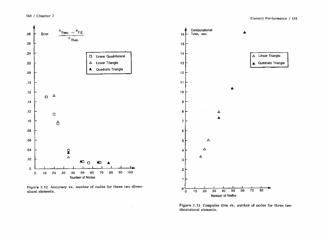
160 I Chapter 7
.28 - Error oTheo. - oF.E.
o Theo.
4 Computational i - Time, sec.
.26 15 I-
.24 14
.22
.20
13
12
.I8 11
.16 IO
.I4
.12
.lO
0
.08
.06
A 100 m A
0 1 I I I I I I I I I I)
0 10 20 30 40 50 60 70 80 90 100 Number of Nodes
Figure 7.12 Accuracy vs. number of nodes for three two-dimen- sional elements.
L 0 0 1
A
A
A
Element Performance / 161
A
A
A
A
I I I I I I 1 I
0 20 30 40 50 60 70 80 Number of Nodes
Figure 7.13 Computer time vs. number of nodes for three two- dimensional elements.

162 / Chapter 7 Element Performance / 163
Table 7.8 Simple Beam: Variable Mesh Density, Number of Degrees of Freedom
Mesh density 2D-Q4 2D-T3 2D-T6
10 x 5 120 132
10 x 4 110 70 234
9x4 100
6x4 70 48 234
5x3 48 48 154
4x3 40 40 126
3x3 32 32 98
3x2 24 24 70
whereas the other elements [2D-Q4, 2D-&4+, 3D-H8(R), 3D- H 8+(R), P-Q 41 modeled the curved boundary as a series of straight segments.
The variable element density study using the QD , solid ele- ment (3D-H20) shows that although a single element can match the geometry of the beam, the one- and three-element model did not give adequate results. This is due to the extreme ( 90°) arc of the model.
Table 7.9 Simple Beam : Variable Mesh Density, Number of Degrees of Freedom and Computer Runtime
2D-T3 2D-T6 Mesh density DOF/sec DOF/sec
10 x 4 701’7.6 234/30.1
5x3 4815.0 154J22.5
4x3 4014.3 126/16.2
3x3 3213.2 98/10.5
3x2 2412.6 7017.2
May Be Modeled with Plate/Beam/2D/3D Solid Elements 90 degree Arc Outer Radius = 4.32 Inner Radius = 4.12 Thickness = 0.1 Young’s Modulus = 1 ,OOO,OOO Poisson’s Ratio = 0.3 Unit Loading Applied at Free End - In Plane and out of Plane
Figure 7.14 Curved-beam benchmark case.
7.5 TWISTED-BEAM BENCHMARK CASE
This case was also taken from the MacNeal-Harder paper [ 11. Di- mensions of the beam are shown in Figure 7.18. The dimensions are length = 12.0, width = 1.1, depth = 0.32. There is a 90° twist along the length. Young’s modulus = 29,000,000, Poisson’s ratio = 0.22, and there is unit loading at the tip in both in-plane and out -of -plane directions.
The exact solution is
In-plane displacement (unit loading) = 0.005424
Out-of-plane displacement (unit loading) = 0.001754
Results are presented as normalized displacements. Tests were run with six different element types with a pattern
of 12 elements along the length and two elements across the width. The results are given in Table 7.11. In addition, the element

164 I Chapter 7 Element Performance / 165
density was varied for the 3D-H8+(R) and P-T3 elements (Fig- ures ‘7.19 and ‘7.20) and the results given in Table 7.12.
The results show that, for the 12 x 2 element pattern, all ele- ment types with the exception of the LD solid [3D-H8(R)] gave good results. The LD solid element was, again, overstiff and gave unacceptable results. This twisted-beam case allows for a study of the effects of distortion (over B” of warping per ele- ment) . A comparison of the results of this case with the results of the baseline, square beam given in Table 7.5 shows compa- rable results with no significant degradation in accuracy due to the warping in the twisted-beam case, with the exception of the LD solid [ 3D-H8(R) ] element. The elements that gave acceptable results for the square beam case still gave acceptable results for the twisted-beam case.
6x1 Pattern of &Node Solid Elements 12x2 Pattern of b-Node Solid Elemenb
Figure 7.16 Curved-beam three-dimensional models. Figure 7.15 Curved-beam two-dimensional model.
In the case of the plate elements, both the quadrilateral and triangular elements were run. The triangular elements, by def- inition, do not have any warping. Table 7.11 shows that for the 12 x 2 gridwork for quadrilaterals (12 x 4 for triangles) , there was no significant advantage to the triangular elements despite the fact that there were twice as many triangles as quadrilaterals used in the models. In fact, the triangular element showed an almost 20% error in the case of in-plane loading.
Table 7.12 gives the results for variable element density for two element types, the P-T3 plate and the 3D-H8+(R) solid. These results show that for the in-plane loading condition, there was little variation in accuracy for the plate element and only a significant difference in results for the solid element when the mesh was reduced to three elements. These results show that both elements approach a point of being about 20% understiff for the solid element and 10% for the solid element.

166 I Chapter 7
6x1 Pattern of 4-Node Plate Elements
6x1 Paffern of Beam Elements
Figure 7.17 Curved-beam plate and beam models.
The solid element showed that with more elements, the overall stiffness of the model decreases, which is generally the case for most elements. This variation in normalized displacement from 0.785-1.096 for the in-plane loading may give the misleading impression that there is an optimum number of elements for this model, beyond which an increase in the number of elements causes a decrease in accuracy. For this particular case, there is an ap- parent optimum mesh of 6 x 1 x 1 , which gives a normalized dis- placement of 1.001, i.e., 0.1% from the theoretical solution. It is important to recognize that this crossover point is a combina- tion of two phenomena: (1) This particular LDADS element con- verges to high displacement results for this model under this loading condition, and (2) the decrease in flexibility as a func- tion of the decreasing number of elements.
For the out-of-plane loading condition, the plate element was slightly understiff in the limit, but overstiff for the coarsest model. For the solid element, the trend was, once again, in- creased flexibility as a function of the number of elements. In
Element Performance / 167
Table 7.10 Results of Curved-Beam Test Cases
Element type Mesh density
Normalized displacement
In plane Out of plane
2D-Q4
2D-Q4+
3D-H8
3D-H8+(R)
3D-H8+(S)
3D-H20
P-Q4
P-Q8
B-2
6x1 0.244 6x2 0.737
12 x 1 0.244 12 x 2 0.247
3x1 0.186 6x1 0.824 6x2 0.822
12 x 1 0.998 12 x 2 0.996
6x1
3x1 6x1
12 x 1
6x1
1x1 3x1 6x1
3x2 6x1 6x2
12 x 1 12 x 2
0.073
0.439 0.935 1.004
0.990 0.849
0.009 0.309 0.875 0.946
0.186 0.833 0.951 0.822 0.998 0.996
6x1
6x1
1.007 0.971
0.904 0.973
this loading condition, however, the element was still somewhat overstiff in the limit. In contrast to the in plane loading condi- tion that was 9.6 over the theoretical displacement, the out-of- plane loading condition gave results 11.4% below the theoretical displacement. There was a fairly uniform convergence of dis- placement as a function of element density from 0.573--0.886.

168 / Chapter 7 Element Performance / 169
\ \ I
\ I I
May Be Modeled with Solid or Plate Elements Length = 12.0 Width = 1 .I Depth = 0.32 90 degree Twist Young’s Modulus = 30,000,OOO Poisson’s Ratio = 0.3 Unit Loading at Free End - in Plane and out of Plane
Figure 7.18 Twisted-beam benchmark case.
7.6 RECTANGULAR PLATE BENCHMARK CASE
This case is taken from the MacNeal-Harder paper [ll. This model is of two simple rectangular plates, each with two sets of boundary constraints: simply supported and clamped. The plates are shown in Figure 7.21. Their dimensions are 2 x 2 and 2 x 10 to give two different geometries. The thickness is 0.0001 for the models using plate elements and 0.01 for the solid-element models. Young’s modulus is 17,420,OOO and Poisson’s ratio 0.3. Two Ioad- ing conditions are applied, a uniform loading of q = 0.0001 force/area and a concentrated loading, at the centroid of 0.0604 force.
Table 7.11 Results of Twisted-Beam Test Cases: Six Element Types, 12 x 2 Element Grid Pattern
Normalized displacements
P-Q4 P-T3 P-Q8 3D-H8 3D-H8+(S) 3D-HZ0
In plane 0.993 1.198 0.998 0.336 0.938 0.991
Out of plane 0.985 0.998 0.998 0.202 0.977 0.995
Figure 7.19 Twisted-beam three-dimensional solid model.
Models are formed with four different element types; two plate elements, P-Q4 and P-Q8; and two solid elements, 3D-H8+(R) and 3D-H20. For each of the element types, four element densities are used: 2 x 2, 4 X 4, 6 x 6, and 8 X 8. The model is quarter- symmetric so that the element densities refer to the number of the elements in the quarter of the plate.
The theoretical solution is taken from Timoshenko [ 21 and is given in Table 7.13.
Results in terms of normalized displacements at the center of the plate are given in Table 7.14 for the 2 x 2 plate and in Table 7.15 for the 2 x 10 plate. The results show good accuracy with X>oth the plate elements for both geometries for the uniform load- ing, simply supported cases. For the concentrated load with

170 I Chapter 7 Element Performance / 171
Figure 7.20 Twisted-beam plate model.
Table 7.12 Results of Twisted-Beam Test Cases: Two Element Types, Variable Mesh Density
Mesh density P-T3 3D-H8+(R) 3D-H8+(S)
In plane 12 x 4 x 1 1.198 12 x 2 x 1 1.096 0.983 12 x 1 x 1 1.077
6x2~1 1.189 1.062 6x1~1 1.001 3x2~1 1.180 0.945 3X1X1 0.785
Out of plane 12 x 4 x 1 1.042 12 x 2 x 1 0.998 0.886 0.977 12 x 1 x 1 0.871 6x2~1 0.930 0.838 6~1x1 0.792 3X2X1 0.798 0.685 3X1X1 0.573
Quarter-Symmetric Model
a = 2.0 b = 2.0 or 10.0 Thickness = 0.01 (solid elements) or 0.0001 (plate elements)
Figure 7.21 Rectangular plate benchmark case.
Table 7.13 Theoretical Displacements for a Rectangular Plate
2 x 2 Plate Simply supported
Clamped
Displacement at center of plate
Uniform loading Concentrated load
4. 062a 11.60
1.26 5.60
2 x 10 Plate Simply supported 12.97 16.96
Clamped 2.56 7.23
a4.062 is the theoretical displacement for the plate-element model; 4.062 x 1O-6 is the displacement for the solid-element model. The thickness of the solid-element model is 100 times greater than that of the plate-element model. Source: Ref. 2.
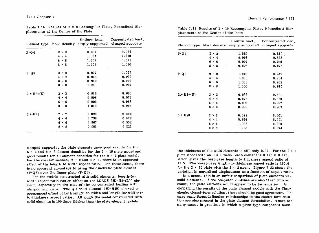
172 / Chapter 7 Element Performance I 173
Table 7.14 Results of 2 x 2 Rectangular Plate, Normalized Dis- placements at the Center of the Plate
Uniform load, Concentrated load, Element type Mesh density simply supported clamped supports
P-Q4 2x2 0.981 0.934 4x4 1.004 1.010 6x6 1.003 1.012 8x8 1.002 1.010
P-Q8 2x2 0.927 1.076 4x4 0.996 0.969 6x6 0.999 0.992 8X8 1.000 0.997
3D-H8+(S) 2x2 0.989 0.885 4x4 0.998 0.972 6x6 0.999 0.988 8x8 1.000 0.994
3D-H20 2x2 0.023 0.002 4x4 0.738 0.072 6x6 0.967 0.552 8x8 0.991 0.821
Table 7.15 Results of 2 x 10 Rectangular Plate, Normalized Dis- placements at the Center of the Plate
Uniform load, Concentrated load, Element type Mesh density simply supported clamped supports
P-Q4 2x2 1.052 0.519 4x4 0.991 0.863 6X6 0.997 0.940 8x8 0.998 0.972
P-Q8 2x2 1.223 0.542 4x4 1.003 0.754 6x6 1.000 0.932 8x8 1.000 0.975
3D-H8+(S) 2x2 0.955 0.321 4x4 0.978 0.850 6x6 0.990 0.927 8x8 0.995 0.957
3D-H20 2x2 0.028 0.001 4x4 0.693 0.041 6x6 1.066 0.220 8x8 1.026 0.374
clamped supports, the plate elements gave good results for the 6 x 6 and 8 x 8 element densities for the 2 x 10 plate model and good results for all element densities for the 2 x 2 plate model. For the coarser meshes, 2 x 2 and 4 x 4, there is an apparent effect of the length-to-width aspect ratio. For these cases, there is no apparent advantage to using the quadratic plate element (P-Q8) over the linear plate (P-Q4).
For the models constructed with solid elements, length-to- width aspect ratio has an effect on the LDADS [3D-H8+(R)] ele- ment, especially in the case of the concentrated loading with clamped supports. The QD solid element (3D-H20) showed a pronounced effect of both length-to-width and length (or width-)- to-thickness aspect ratios. Although the model constructed with solid elements is 100 times thicker than the plate-element models,
the thickness of the solid elements is still only 0.01. For the 2 x 2 plate model with an 8 x 8 mesh, each element is 0.125 x 0.125, which gives the best-case length-to-thickness aspect ratio of 12.5. The worst-case length-to-thickness aspect ratio is 100.0 for the 2 x 10 plate with the 2 x 2 mesh. Figure 7.22 shows the variation in normalized displacement as a function of aspect ratio.
In a sense, this is an unfair comparison of plate elements vs. solid elements. If the computer runtimes are also taken into ac- count, the plate elements would appear to be far superior. In comparing the results of the plate element models with the Timo- shenko closed-form solution, there should be good agreement. The same basic force/deflection relationships in the closed-form solu- tion are also present in the plate element formulation. There are many cases, in practice, in which a plate-type component must

Element Performance / 175
be modeled with three-dimensional solid elements as part of a larger model with fully three-dimensional geometry details that require the use of three-dimensional solid elements. This case illustrates some of the capabilities and shortcomings of the use of solid elements in modeling flat plates.
It is interesting to note the effect of loading and constraint conditions on model accuracy. A comparison of the two columns in either Table 7.15 or 7.16 shows these effects. In most cases, the models tended to underpredict the theoretical displacements. However, in a few cases (P-Q8 element), the models overpre- dieted the displacement for one loading/constraint case and un- derpredicted the displacement for the other case with the same element density and geometry. When these effects are taken into account with the aspect ratio effects, it becomes clear that the performance of a particular element cannot be completely de- duced from an isolated test.
7.7 SCORDELIS-LO ROOF BENCHMARK CASE
This case was first published by Scordelis and Lo in 1969 [3], discussed by Zienkiewicz in his text [ 41, later included in the MacNeal and Harder proposed benchmark set [ 11, and is be- coming a classic among finite element benchmark cases.
The structure and model are shown in Figure 7.23. It is a curved-plate-type structure, length = 50, thickness = 0.25, and the “width” specified as a 25.0 radius with an 80° included arc. The Young’s modulus is 432,000,OOO and Poisson’s ratio 0.0. The loading is -90.0 in the vertical (Z) direction. One-quarter of the structure is included in the model with symmetry bound- ary conditions applied on the cut boundaries. Axial and radial displacements are constrained to 0 on the curved boundaries.
Calculations are run using four element types; two plate ele- ments, P-Q4 and P-Q8; and two solid elements, 3D-H8+(R) and 3D-H20. The results are presented in Table 7.16.
The length-to-thickness aspect ratio varies between 20 and 100, which is about the same range as the models for the flat rectangular plate. It comes as no surprise that the results for the solid-element models in the coarsest mesh are poor. The re- sults for the QD solid element (3D-H20) are similar to the results for the flat rectangular plate case. It is interesting and some- what disappointing to note that the QD solid element underper- formed the LDADS element for all meshes. With the additional
174

176 I Chapter 7 Element Performance / 177
Boundaries: Radial and Axial Constraints on Curved Free Boundaries Symmetry on Cut Boundaries
Radius = 25.0 Thickness = 0.25 Length = 50.0
Young’s Modulus = 432,000,OOO Poisson’s Ratio = 0.0 Distributing Loading = 90.0 per unit area in -z direction
Figure 7.23 Scordelis-Lo benchmark case: Concrete cylindrical shell quarter-symmetric model.
midside node, the QD solid is able to model exactly a cylindrical surface. The LDADS element must approximate the surface as a series of flats. The logical explanation is that the length-to- thickness aspect ratio affects the QD solid more adversely than the LDADS solid element.
Both plate elements performed well with virtually identical re- sults at the more refined meshes. The QD plate element (P-Q 8) converges to within 0.2% of the theoretical value with the 6 x 6 mesh and, therefore, cannot show any more improvement with
Table 7.16 Results of Scordelis-Lo Roof, Normalized Displacements at the Center of the Free Edge
Element type Mesh density Uniform load,
simply supported
P-Q4 2x2 1.376 4x4 1.050 6x6 1.018 8x8 1.008
10 x 10 1.004
P-Q8 2x2 1.021 4 x-4 0.984 6x6 1.002 8x8 0.997
10 x 10 0.996
2x2 1.320 4x4 1.028 6x6 1.012 8x8 1.005
2x2 0.092 4x4 0.258 6x6 0.589 8x8 0.812
3D-H8+(S)
3D-H20
more refined meshes. With the coarser meshes, there can be problems with the QD plate elements, such as the P-Q8 when the out -of-plane curvature exceeds a certain limit. A rule-of-thumb limit is that the height of the arc for each element should not be greater than 10% of the chord. In this case, the ratio is 0.088 for the 2 x 2 mesh (i.e., each element including a 20° arc) and 0.017 for the 10 x 10 case. This 10% limit number corresponds to a 22.5O arc.
7.8 SPHERICAL SHELL BENCHMARK CASE
This spherical shell benchmark case gives a model with double curvature. The theoretical solution is given by Morely and Morris

178 I Chapter 7 Element Performance / 179
[ 51 for a complete spherical shell. The case as it is presented here was modified by MacNeal and Harder to include a hole at the top of the sphere to avoid the need for triangular elements [ll .
The structure and model are shown in Figure 7.24. The di- mensions of the hemisphere are radius = 10.00 and thickness = 0.04 with a hole at the top subtended by an 18O angle. Young’s modulus is 6.825 x 10’ and Poisson% ratio is 0.3. Forces are ap- plied at four points, 90“ apart, along the free edge of the hemi- sphere in the radial direction, as shown. The forces have a mag- nitude of 2.0, but alternate in sign. One-quarter of the hemi- sphere is modeled with symmetry boundary conditions along the cut boundaries. Models are constructed from four element types; two plate elements, LD (P-Q4) and QD (P-Q@; and two solid ele- ments, LDADS [ 3D-H8+(R)] and QD (93D-H20). Five element densities are used for the plate elements and three element den- sities for the solid elements.
The theoretical solution given by Morley and Morris for dis- placement at the point of force application is 0.0924 for a com- plete hemisphere. MacNeal and Harder used a value of 0.0940 for the hemisphere with a hole at the top.
Results are presented in Table 7.17. A comparison of the two plate elements shows that the LD element (P-Q4) showed good behavior for all element densities. The QD element showed poor performance for the coarse element densities with a uniform convergence at the finer element densities and gave similar re- sults for the finest, 12 x 12 mesh. The behavior of the QD plate is substantially worse in this case than in the cases of the rec- tangular plate and the Scordelis-Lo roof. The explanation is the double curvature of the elements. For the coarsest, 2 x 2 mesh, each element must span 45O along the equator (free sur- face) and 36O along the symmetric boundaries.
The solid elements showed a similar pattern with the LDADS element [3D-H8+(R)] giving better performance than the QD ele- ment (3D-H20). The LDADS element gave a good result for the 12 x 12 mesh. The QD element gave unacceptable results for all meshes.
The same comments regarding the selection of plate elements vs. solid elements that were made for the rectangular plate also apply to the Scordelis-Lo roof and the spherical shell. In model- ing plate-type structures, plate elements will perform at least as well as solid elements. When the computer runtime is also taken into account, plate elements become the clear winner. The choice to use solid elements will be necessitated by the need to model details such as lugs, fitting, ports, gussets, ribs, etc. and
Hemispherical Shell with Hole at Top QuarterSymmetric Model Radius = 10.0 Thickness = 0.04 90 degree Arc Young’s Modulus = 68,250,OOO Poisson’s Ratio = 0.3 Boundaries: Symmetric on Cut Boundaries
Top and Bottom Boundaries Free Loading: Point Loads at Quadrant Points
F=2.0 asShown
Figure 7.24 Spherical shell benchmark case.
obtain accurate and detailed stresses. In such cases, an alterna- tive to solid elements is the use of plate elements throughout with a second, refined model of the geometric details. Refined models are discussed in more detail in Chapter 9.

180 I Chapter 7 Element Performance I 181
Table 7.17 Results of Spherical Shell Test Case, Normalized Radial Displacement at the Point of Load Application
Element type
P-Q4
P-Q8
3D-HB+(S)
3D-H20
Mesh density
2x2 4x4 6x6 8x8
10 x 10 12 x 12
2x2 4x4
6x6 8X8
10 x 10 12 x 12
4x4 8x8
12 x 12
4x4 8x8
12 x 12
Uniform load, simply supported
0.972 1.024 1.013 1.005 1.001 0.998
0.025 0.121
0.494 0.823 0.955 0.955
0.039 0.730 0.955
0.001 0.776 0.972
7.9 THICK-WALLED CYLINDER
This geometrically simple problem is intended to test the ability of the various elements to model a nearly incompressible material with a Poisson’s ratio approaching 0.5. This problem is taken from the MacNeal-Harder set of test cases [ 11. The structure and model is shown in Figure 7.25. The cylinder has an inner radius of 3.00, an outer radius of 9.00, and a length of 1.00. There is a unit pressure acting on the inner surface. Young’s modulus is set to 1000 and Poisson’s ratio is varied as 0.49, 0.499, and 0.4999. A 5 x 1 gridwork representing a loo seg- ment of the cylinder is used for the model.
A theoretical solution is given by MacNeal and Harder [l] and Roark [ 61
wm Plane Strain Model for Nearly Incompressible Material Inner Radius = 3.0 Outer Radius = 9.0 Thickness = 1 .O Young’s Modulus = 1000. Poisson’s Ratio = 0.49 0.499 0.4999 Loading: Unit Pressure on Inner Surface
Figure 7.25 Thick-walled cylinder benchmark case.
(l+~) P R*. inner u = B(R20uter - R2inner) [R *outer /r + (l-2u)r] (7.1)
For this model, the solutions for three values of Poisson’s ratio are
Poisson’s ratio Radial displacement at inner radius
0.49 0.00050399
0.499 0.00050602 0.4999 0.00050623
Eight different element types are used with the three values of Poisson’s ratio as shown in Table 7.18. The same 5 x 1 gridwork is used for all elements. Boundary conditions are specified to represent symmetry along the cut boundaries by permitting dis- placement in the radial direction and constraining against displace- ment in the tangential direction. Plane strain conditions are as- sumed for the two-dimensional and plate elements.
Table 7.18 shows that there is no substantial difference be- tween the LD , LDADS , and QD two-dimensional elements, with the LD and QD elements slightly overpredicting displacement by the same amount for all cases of Poisson’s ratio and the LDADS element underpredicting slightly. -This is to be expected be- cause. the added displacement shapes only affect the element’s

182 I Chapter 7 Element Performance / 183
Table 7.18 Results of Thick-Walled Cylinder Test Case, Normalized Radial Displacement at Inner Boundary
Variable Poisson’s ratio
Poisson’s ratio Element type 0.49 0.499 0.4999
2D-Q4 1.019 1.020 1.020
2D-Q4+ 0.988 0.982 0.931
2D-Q8 1.036 1.037 1.037
P-Q4 0.846 0.359 0.053
P-Q8 1.000 0.997 0.967
3D-H8 0.936 0.809 0.771
3D-H8+(S) 0.986 0.986 0.986
3D-H9+(R) 1.025 1.026 1.026
3D-H20 0.999 0.986 0.879
performance in bending. In cases of pure tensile or compressive loading, there should be no difference in behavior.
For the three-dimensional solid elements, the LD,ADS element [3D-H8+(R)l showed uniform behavior, whereas the QD element (3D-H20) showed a decrease in accuracy for the case of Poisson’s ratio equal to 0.4999 and the LD element [3D-H8(R)l showed a decrease in accuracy across all cases of Poisson’s ratio. The LD plate element (P-Q4) had difficulty with the cases of Poisson’s ratio equal to both 0.499 and 0.4999.
7.10 ROTATING DISK BENCHMARK CASE
This case of a hyperbolic disk rotating about its axis, which is not part of the MacNeal-Harder set, gives a case of nonuniform body (centrifugal) forces and an opportunity to investigate the
mass properties of the various element types. This type of prob- lem has practical interest in turbomachinery applications, which provide the basis for the theoretical solution 171. Timoshenko [ 81 offers a closed-form solution and discussion.
The disk in this benchmark case is described by Roark [6] and has a hyperbolic profile described as
t = era (7.2) where t is the disk thickness at radius, r and c and a are con- stants. The disk used in this benchmark case is shown in Fig- ure 7.26, where c = 4.819 and 1 - -0.6826 so that t - 3.00 in. at r 1 (inner radius) and t = 1.00 in. at r . The Young’s modulus is 30,000,OOO psi, Poisson’s ratio 0.3, and the weight density 0.279 lbflin. 3. The rotational speed is 377 radlsec.
The theoretical solution for stress is taken from Roark [6] and is based on the solution by Stodola [ 71. Roark’s notation is used.
E cs r = 2 [ (3+u)Fr* + (m,+u)Arml-’ + (m2+u)Brm2-ll psi
1-u (7.3)
at = *[(1+3u)Fr* + (l+mlu)Arml-’ + (l+m2u)Brm2-‘1 psi (7.4)
where
ur and ot = radial and tangential (hoop) stresses E = Young’s modulus, 30,000,OOO psi IJ = Poisson’s ratio, 0.3 r = the distance from the centerline
F = -(l-v*) 6 w* I 386.4 E[8 + (3+u) al
(7.5)
6 W
a
= the weight density, 0.279 lbf/in.3 = the rotational speed, 377.0 radlsec = the exponent from the hyperbolic thickness ex-
pression, as shown above, -0.6826
m2
a =--- (
2 - 2
,“2 al.l 1
+ 1
112
a =--+ 2 ( ;I--au+1 1
112
(7.6)
(7.7)
A and B are constants derived by using known radial stresses at the boundaries and solving Equation 7.5 as a set of two simul- taneous equations with r = rl and r = r2 together with the appro- priate radial stresses. In this case, radial stresses at the bore

184 / Chapter 7 Element Performance / 185
The following values of A and B are obtained.
A = 5.30251 x 1O-4
B = 3.34593 x 1O-4
These constants satisfy the boundary conditions of ur = 0.0 at r = 2.00 and 10.00. Radial and tangential stresses are calcu- lated at two other points that correspond to element centroid lo- cations for two gridwork patterns used in the test case.
r = 2.4 (centroid for 20-element gridwork) or = 866.99 psi at = 4974.46 psi
r = 2.8 (centroid for B-element gridwork) cl r = 1424.97 psi at = 4434.14 psi
It should be noted that the solution is extremely sensitive to the constants A and B that must be precisely calculated to at least five significant figures. A simple calculation with a hand calculator may not be adequate to obtain A and B with sufficient precision. It is recommended that in order to use Equations 7.3- 7.7 to calculate other comparison cases, a computer should be used to achieve the required precision.
Three axisymmetric element types are used in the models: LD (2D-Q4), LDADS (2D-&4+), and QD (2D-Q8). All three element types are used with a 5 x 1 gridwork as shown in Figure 7.27. The LD and LDADS elements are also used with a 2 x 10 grid- work. Stresses are calculated at the element centroids for com- parison with the theoretical solution. A limiting case of a single element was also run. In the single element model, however, the disk cross section is a simple tapered section and not a hyper- bola .
The results of normalized centroidal stresses, i.e., calculated FEA stress divided by the theoretical stress at the same radius, are presented in Table 7.19. These results show that calculation of tangential (hoop) stress is consistently more accurate than the calculation of radial stress. The tangential stress results are good with both the 5-element and 20-element models for all ele- ment types. For radial stress, the LD element ( 2D-Q 4) gave the best results, nominally 8% low, with the LDADS element (u>-&4+) giving results about 13-19% low. The quadratic element under- predicted stress by about 12%. It may appear somewhat sur- prising that the QD element did not perform better, consider- ing that it should approximate the hyperbolic surface with a
Rotating Disk Axisymmetric Model Hyperbolic Profile Inner Radius = 2.0 Outer Radius = 10.0 Rotational Speed: 3600 rpm Young’s Modulus = 30,000,000 Poisson’s Ratio = 0.3
3600 !rpm
Figure 7.26 Hyperbolic disk benchmark case.
bore and at the outside diameter, set equal to zero, are used as boundary conditions.
r = rl = 2.00, Url = 0.0
r = r2 = 10.00, a,2 = 0.0
186 I Chapter 7 Element Performance 1 187
Table 7.19 Results of Rotating Hyperbolic Disk, Normalized Radial and Hoop Stress (rotational speed = 377 radlsec)
Element Number of Radial Radial Hoop Total type elements location stress stress mass
2D-Q4 la 2.90 1.4587 1.1297 2.617 5 2.80 0.9162 0.9712 1.931
20 2.40 0.9219 0.9688 1.918
2D-Q4+ 5 2.80 0.8109 0.9556 1.931 20 2.40 0.8655 0.9761 1.918
SD-Q8 5 2.80 0.8845 0.9977 1.931
aThis is a limiting case. With only one element, the disk has a simply tapered cross section and not a hyperbola.
2D Axisymmetric Elements
7.11 SUMMARY
One Node Constrained in the Axial Direction Rotational Speed = 377 radianskec (3600 rpm) Axisymmetric Model - No Radial Constraint Necessary
Figure 7.27 Hyperbolic disk axisymmetric model.
second-order curve. A comparison of total mass moment of each model is given in Table 7.20 and shows that despite the fact that the sides of the QD element can model a curved surface, the mass moment numbers show no difference between the two, 5-element linear and LDADS models and the QD model. The two, 20-node models showed slightly lower mass moments as expected because the elements will always overpredict volume (and mass) on a con- cave surface.
The original title for this chapter was “Properties of the Elements.” However, this sort of a title is misleading because the behavior of an element is not only a function of the element itself, but of equal importance are the type of loading, type of constraints, and type and degree of distortion. A review of the various cases shown here with the same elements shows that it is not possible to pub- lish sets of accuracy numbers for specific elements, isolated from the model to which they will be applied.
The proposed set of benchmark cases by MacNeal and Harder has provided finite element users with an excellent set of simple standards against which to check various finite-element codes and elements. The value of the work published by MacNeal and Harder is not so much the actual performance numbers on the ele- ments that they tested, but rather the setting forth of a simple, yet realistic set of problems against which any user can test his code.
When a finite element user has a new problem to model and is faced with the step of selecting an element type(s) and element density to use, it is recommended that one of the benchmark problems, which most dosely represents the actual case, be

188 I Chapter 7
selected and simple models with variable element densities and element types be run. The published performance numbers can be used for guidance, but the user should repeat the benchmark runs with his particular code, version, and selected elements to investigate the element performance. The problems in the bench- mark set are simple enough that a case can be set up and run for a series of element densities with a minimal amount of labor and computer time.
Two other excellent sources of potential benchmark cases are Roark’s Formulas for Stress and Strain [ 61 and Timoshenko’s Strength of Materials 181. These two sources offer the best col- lections of closed-form solutions to practical solid mechanics prob- lems against which to test finite-element models.
REFERENCES
1.
2.
3.
4.
5.
6.
7.
8.
MacNeal, R. H. and R. L. Harder, “A Proposed Set of Prob- lems to Test Finite Element Accuracy,” Finite Elements in Analysis and Design, No. I, North-Holland, Amsterdam, 1985. Timoshenko, S. and S . Woinowsky-Krieger , Theory of Plates and Shells, 2nd ed. , McGraw-Hill, New York, 1959, pp. 120, 143, 202, 206. Scordelis, A. C. and K. S. Lo, “Computer Analysis of Cylin- drical Shells ,I’ Journal of the American Concrete Institute, No. 61, 1969, pp. 539-561. Zienkiewicz, 0. C . , The Finite Element Method, McGraw-Hill, London, 1977, p. 417. Morely , L. S. D. and A. J. Morris, “Conflict Between Finite Elements and Shell Theory, It Royal Aircraft Establishment Report, London, 1978. Roark, R. J. and W. C. Young, Formulas for Stress and Strain, 5th Ed., McGraw-Hill, New York, 1975. Stodola, A. , Dampf- und Gasturbinen (Steam and Gas Tur- bines) , 6th ed. , 1924, pp. 312-340. Timoshenko , S. , Strength of Materials, Part II, 3rd ed., Van Nostrand, New York.
8
ELEMENT DISTORTION
Finite element models of geometrically complex structures have the potential problem of element distortion. It is known that elements give the best results when they are used in their ideal shape, i.e., equilateral triangles, square quadrilaterals, and three-dimensional solid elements that are perfect cubes. In practice, however, it is nearly impossible to have all elements with perfect shapes. Ele- ments will tolerate ‘a modest amount of deviation from their ideal shape without any noticeable decrease in accuracy. Beyond a certain point of distortion, element stiffness and stress accuracy drop off dramatically. What constitutes an acceptable amount of distortion and what defines the point of accuracy rolloff are diffi- cult questions whose answers will be different for every combina- tion of element type, constraints, and loading. This determination is not apparent in a casual examination of any given element deri- vation and requires a detailed theoretical analysis beyond the pa- tience of most finite element users. The best discussions of the effects of distortion on various element types are given-by Cook
189
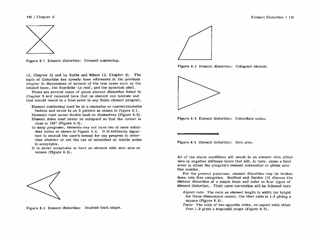
190 I Chapter 8 Element Distortion / 191
X Figure 8.1 Element distortion: Crossed numbering.
(1, Chapter 5) and by Bathe and Wilson (2, Chapter 4). The topic of distortion has already been addressed in the previous chapter in discussions of several of the test cases such as the twisted beam, the Scordelis-Lo roof, and the spherical shell.
There are several cases of gross element distortion listed in Chapter 5 and repeated here that no element can tolerate and that should result in a fatal error in any finite-element program.
Element numbering must be in a clockwise or counterclockwise fashion and never in an X pattern as shown in Figure 8.1.
Elements must never double back on themselves (Figure 8.2). Element sides must never be collapsed so that the corner is
close to 180° (Figure 8.3). In many programs, elements may not have two or more coinci-
dent nodes as shown in Figure 8.4. It is extremely impor- tant to consult the user’s manual for any program to deter- mine whether or not the use of coincident or double nodes is acceptable.
It is never acceptable to have an element with zero area or volume (Figure 8.5).
Figure 8.2 Element distortion: Doubled-back shape.
Figure 8.3 Element distortion: Collapsed element.
Figure 8.4 Element distortion : Coincident nodes.
. .
Figure 8.5 Element distortion: Zero area.
All of the above conditions will result in an element with either zero or negative stiffness terms that will, in turn, cause a fatal error in either the program’s element subroutine or global solu- tion routine.
For the present purposes, element distortion may be broken down into five categories. MacNeal and Harder [3] discuss the element distortion of a simple beam and refer to four types of ,element distortion. Their name convention will be followed here
Aspect ratio The ratio an element length to width (or height for three-dimensional cases) , the ideal ratio is 1.0 giving a square (Figure 8.6).
Taper The ratio of two opposite sides, an aspect ratio other than 1.0 gives a trapezoid shape (Figure 8.7).

192 I Chapter 8 Element Distortion / 193
II Ta AspectRatio=a/b
Figure 8.6 Aspect ratio definition.
Skew angularity The element vertex angles, ideal is 90” for a quadrilateral and 60° for a triangle (Figure 8.8).
Warping Applies to plate elements, the measure of the distance that a node lies out of the plane defined by the other three nodes of a quadrilateral plate.
Bow Applies to plate elements that are curved and form part of a cylindrical surface. Bow refers to the ratio of the height of the arc to the chord length.
8.1 SIMPLE BEAM: ONE LAYER OF ELEMENTS
MacNeal and Harder [3] use a simple beam with three-element pat- terns to test the effects of moderate distortion on the accuracy of several element types. The beam is 0.2 wide, 0.1 thick, and 6.0 long. Young’s modulus is l.OE’ and the Poisson’s ratio 0.3. The
a
t-l
A Taper Ratio = a/b
lb
Figure 8.8 Skew angularity definition.
\ \ \ I I I I I I
Figure 8.9 Rectangular beam: Baseline model.
three-element patterns are shown in Figures 8.9-8.11. The first used a single layer of rectangular elements across the section, the second adjusted the nodes to give a skew angle of 45O (pa- rallelogram elements), and the third adjusted the nodes to give a taper ratio of 0.67 (trapezoidal elements).
Figure 8.10 Rectangular beam : Parallelogram elements.
\ \ \ 1
Figure 8.7 Taper ratio definition. Figure 8.11 Rectangular beam : Trapezoidal elements.

194 / Chapter 8 Element Distortion / 195
Four loading conditions are applied, axial tension, shear load- ing at the tip in both the in-plane and out-of-plane directions to give a combined direct and bending loading, and a twist applied to the tip of the beam. Unit load amplitude is applied in all cases. Theoretical tip displacements are obtained from beam theory
Tension tip displacement = 3 x lo- 5 In plane tip displacement = 0.1081 Out of plane tip displacement = 0.4321 Twist tip displacement = 0.03208
The results of the MacNeal-Harder study along with results from two additional three-dimensional solid elements are given in Table 8.1. The results show good performance for all elements in the tensile loading case. For a simple geometry and uniaxial tensile loading, it is expected that all elements should give good results. For the cases of in-plane and out-of-plane shear loading at the tip, the results are generally good with a few exceptions. The LD plate (P-Q4) element did not do well with in-plane loading when the elements are distorted in the parallelogram and trape- zoidal shapes . This is not a problem with the QD plate (P-Q8) as it gave consistently good performance for all three gometries and load conditions. The QD plate can support a linear stress distribution across its section.
8.2 EFFECT OF NUMERICAL INTEGRATION ORDER
The three LDADS three-dimensional solid elements used in the simple beam test case and shown in Table 8.1 gave different re- sults. Although all three of these elements can be classified as LDADS three-dimensional solid elements, there are differences in the numerical integration procedures used to produce the stiff- ness matrices. In forming the element stiffness matrix, it is re- quired to integrate element stiffness over the element volume. The common numerical integration techniques, such as Gauss quadrature or the Newton-Cotes formula, requires that a stiff- ness function be evaluated at a number of points within the ele- ment volume. The values of this function are then multiplied by appropriate weighting factors and summed to give the value of the integral.
The order of numerical integration, i.e., the number of points to be used, may be selected to optimize the accuracy vs. computer

196 I Chapter 8 Element Distortion / 197
time for the elements. Bathe and Wilson 121 point out that for a polynomial of order n (n = 1 for a LD element, n = 2 for a QD element), the Newton-Cotes formula requires n + 1 points and Gauss quadrature integration requires 2n - 1 to exactly inte- grate the function. For example, a LD or LDADS three-dimen- sional solid element integrated by Gaussian quadrature would re- quire a minimum of 2 x 2 x 2 integration points, but 3 x 3 x 3 integration points would give an exact integration. Bathe and Wilson [ 21 and Cook [l] state that exact integration gives an upperbound on stiffness, i. e . , the finite-element method in- herently overpredicts stiffness and, in general, converges to an overstiff solution when exact numerical integration is used. The use of reduced integration order, e.g. , 2 x 2 x 2 integra- tion of a three-dimensional solid element rather than 3 x 3 X 3, generally gives reduced stiffness. In many cases, the use of a reduced integration order can be used to compensate for the in- herent overstiffness of the element and give superior results.
Reduced integration order has the second benefit of substan- tially reducing computer time. Element formulation times and ele- ment stress recovery times are virtually a linear function of the number of integration points for Guassian quadrature, so that the difference between 2 x 2 x 2 (8 points) and 3 x 3 x 3 (27 points) is a factor of 8/27 or 0.296. When the time for equation solution and overhead routines are included, the total difference for the analysis is about 1: 2.
Reduced integration order, however, has the potential disad- vantage of producing erratic results in cases where the elements are distorted to any degree. Reduced integration order may also cause a singularity in the stiffness matrix that can, in turn, pro- duce useless results. Elements formed with reduced integration order, even when distorted, may produce acceptable results, ac- cording to Cook [ 11, when the element happens to be aligned with a strain field that it can exactly represent. This phenomenon is illustrated by the three three-dimensional solid elements in Table 812. The three LDADS three-dimensional solid elements are
3D-H8+(R) three-dimensional solid element, extra bending shapes, 2 x 2 x 2 reduced integration.
3D-H8+(S) three-dimensional solid element, extra bending shapes, selected reduced integration.
3D-H8+(F) three-dimensional solid element, extra bending shapes, full 3 x 3 x 3 integration.
In addition, two QD elements, 3D-H20 and 3D-H20(R), are in- cluded in Table 8.2. The 3D-H20 element is the 20-node, QD,
Table 8.2 Results of Straight Beam Test Cases (five element types, 6 x 1 element grid pattern)
Square ele- Normalized displacementsa
mentsa 3D-H8+ 3D-II20
Tension 0.988 1.250 In plane 0.994 0.988 Out of plane 0.994 0.988
Rectangular Normalized displacements
elements 3D-H8+ 3D-H8+(S) 3D-H8+(F) 3D-H20 3D-H20(R)
Tension 0.978 0.988 0.978 0.994 0.999 In plane 0.978 0.981 0.978 0: 970 0.984 Out of plane 0.981 0.981 0.973 0.961 0.972 Twist 0.910 0.904 0.911
Parallelogram Normalized displacements
elements 3D-H8+ 3D-H8+(S) 3D-H8+(F) 3D-H20 3D-H2O(R)
Tension 0.970 0.989 1.007 0.994 0.999 In plane 0.666 0.080 0.638 0.967 0.994 Out of plane 0.562 0.055 0.544 0.941 0.961 Twist 0.904 0.913 0.918
Trapezoidal Normalized displacements
elements 3D-H8+ 3D-H8+(S) 3D-H8+(F) 3D-H20 3D-H20(R)
Tension 1.015 0.989 1.007 0.994 0.999 In plane 0.097 0.069 0.655 0.964 0.964 Out of plane 0.061 0.051 0.045 0.964 0.964 Twist 0.906 0.904 0.918
aFrom baseline case, Table 7.5.
three-dimensional solid, isoparametric solid with full 3 x 3 x 3 integration. The 3D-H20(R) element is the 20-node, QD, three- dimensional solid with reduced integration.
Table 8.2 is a subset of Table 8.1 with the addition of the base- line performance data on the 3D-H8+(R) element taken from Table

198 I Chapter 8 Element Distortion / 199
7.5. In this case, there is no substantial difference in accuracy between the perfectly cubic elements of the baseline case from Table 7.5 and the rectangular elements with a length-to-thick- ness aspect ratio of 0.1/l = 0.1000. This can be attributed to the fact that the results for both element shapes are close to the theoretical solution. All elements gave good results in simple tension regardless of the element shape. This is due to the fact that the elements are representing a constant, uniaxial stress field, and t as Cook points out, LD or LDADS elements should be able to represent a constant stress condition even with distor- tion. When the elements are called on to represent a stress gra- dient , especially a reversed stress gradient, the LDADS elements begin to show unacceptable results. The QD elements, by virtue of the fact that they can exactly represent a linear variation in strain and stress within the element, gave good results for these beam bending case with its fully reversed bending stresses.
For the parallelogram elements, the 3D-H8+(R) (2 x 2 x 2 in- tegration) and 3D-H8+(F) (3 x 3 x 3 integration) did substan- tially better in bending than the LDADS three-dimensional solid element with selected reduced-order integration 3D-H8+( S) in the two bending cases. The two QD elements gave good results for all load cases.
For the trapezoidal elements, there is a difference in the be- havior for in-plane bending between the 8-node solid element with full 3 x 3 x 3 integration [3D-H8+(F)] and the two 8-node solid elements with reduced integration. For the loading case of out-of- plane bending, all three LDADS elements gave equally poor results.
The 20-node solid element with the reduced integration order gave slightly better results than the same element using full 3 x 3 x 3 integration. All results for the QD elements, and for the most part for all of the elements, showed that the elements are overstiff, as evidenced by most of the ratios being less than 1.0 in Table 8.2. The fact that there is an increase in flexibility with the QD solid element using a reduced integration scheme verifies Cook’s, Bathe and Wilson’s statements that the increased flexibil- ity of less than exact integration helps to balance the inherent overstiffness of the elements.
8.3 SIMPLE BEAM: THREE-ELEMENT LAYERS
A second beam model was set up consisting of three layers of three-dimensional solid elements as shown in Figure 8.12 in order
Completely Constrained
Figure 8.12 Three-layer beam: Baseline model.
to study the combined effects of element skew angularity and as- pect ratio, and the effect of taper ratio. The beam dimensions are 1 x 3 x 7. The Young’s modulus is 30,000,OOO and Poisson’s ratio 0.3. The loading consisted of a set of forces, as shown in Figure 8.12, giving a bending moment at the free end.
Four cases of skew angle, including a baseline case of 90°, are run as follows: 90, 45, 30, and 15O. Four cases of taper ratio, including a baseline case of taper ratio equal to 1.0 are run as follows: 1.00, 0.200, 0.02, and 0.002. For the taper ra- tio investigation, three different elements are used: 3D-H8+(F), 3D-H8+(R), 3D-H8. In the skew angularity test, two element types, 3D-H8+ and 3D-H8(R), are used.

200 I Chapter 8 Element Distortion / 201
Figure 8.13 Three-layer beam: Skew angle/aspect ratio test.
8.3.1 Skew Angle/Aspect Ratio Test
The vertex angles for the top and bottom layer of elements are varied through 90 (perfect), 45, 30, and 15O as shown in Fig- ure 8.13. The results are given in Tables 8.3 for displacements and 8.4 for stresses. These results showed that for the 3D-H8+(F) element, the accuracy did not drop off substantially until the skew ailgle is greater than 60° and the width-to-length ratio is less than 0.22. The LD element 3D-H8(F) showed a uniform dropoff in ac- curacy with a substantial drop from 0.683 to 0.2’70 in normalized stress, going from 60 to 75O.
In these cases of the three-layer beam, the accuracy of stresses at the surface was investigated as well as global displacements. In actual practice, not all elements in a model will have the same degree of distortion as they do in the single-layer beam model. Most of the elements in a typical model will not be badly dis- torted. However, groups of elements in transition areas may
Table 8.3 Results of Straight Beam Distortion Test, Displacement Results (three element types, 6 x 3 element grid pattern, in-plane moment loading)
Taoer test
Normalized displacements
Taper ratio 3D-H8(F) 3D-H8+(F) 3D-H8+(R)
1.000 0.950 1.000 1.000 0.200 0.926 0.999 1.000 0.020 0.790 0.990 1.000 0.002 0.631 0.985 1.000
Skew test
Normalized displacements
Skew angle 3D-H8(F) 3D-H8+(F)
90.0 1.000 1.000 45.0 0.729 0.945 30.0 8.521 0.851 15.0 0.282 0.725
have to be distorted to accommodate element patterns or model geometry. In these cases, the global displacements may not be substantially affected by moderate inaccuracy in the stiffness of a few distorted elements. However, the stress solution may pro- duce stress results in those distorted elements that have a mod- erate error. Although this may be a localized effect in the model, it may be disconcerting in any event.
8.3.2 Taper Ratio Test
The results of the taper ratio study for taper ratios of 1.0 (per- fect), 0.20, 0.02, and 0.002 are shown in Tables 8.3 and 8.4 for displacements and stresses, respectively. The model for the ta- per ratio of 0.02 is shown in Figure 8.14. Displacement results showed that both formulations of the LDADS element gave good results with the maximum error of only 1.5% for the LDADS ele- ment with full 3 x 3 x 3 integration [3D-H8+(F)] and a taper ratio

202 ! Chapter 8
Table 8.4 Results of Straight Beam Distortion Test, Stress Re- sults (three element types, 6 x 3 element grid pattern, in-plane moment loading)
Taper ratio
1.000 0.200 0.020 0.002
Taper test
Normalized stresses
3D-H8(F) 3D-H8+(F)
0.995 1.000 1.133 1.090 1.189 1.149 1.219 1.152
3D-H8+(R)
1.000 1.016 1.035 1.035
Skew angle
90.0 45.0 30.0 15.0
Skew test
Normalized stresses
3D-H8(F) 3D-H8+(F)
0.995 1.000 0.840 1.003 0.683 1.012 0.270 1.140
Figure 8.14 Three-layer beam: Taper ratio
Element Distortion I 203
of 0.002, i.e., effectively wedges on the top and bottom layer of elements. The element with full integration underpredicted dis- placement, whereas the element with reduced integration [ 3D- H8+(R)] gave perfect displacements, to four significant digits, for all taper ratio cases. This shows, again, that the increased flexibility of reduced integration countered the inherent over- stiffness of the element. The linear element (3D-H8), as ex- pected, is overstiff and the most sensitive to taper ratio.
The stress results showed trends that are similar to those of the displacement results. The LDADS element with reduced in- tegration performed the best of the three elements, followed by the LDADS element with full integration and the LD element. All elements overpredicted stress. This may be explained as follows: (1) the effect of a nonzero taper ratio is to make the element over- stiff, (2) this overstiffness is moderated by the center row of elements that have more accurate and flexible stiffness proper- ties, (3) the global displacements are not as small as they would have been if all elements in the beam had the overstiff properties
test.
displacements com- of the top and bottom layer, (4) the global bined with the higher stiffness and stress properties give higher stresses.
The LDADS elements showed a leveling off of error below a ta- per ratio of 0.02. Changing the taper ratio an order of magnitude from 0.02 to 0.002 produced only a 0.3% difference in stress re- sults for the LDADS element with full integration [ 3D-H8+(F)]. There is no change in stress for the LDADS element with reduced integration [3D-H8+(R)] for taper ratios of 0.02 and 0.002. The maximum error for this element is only 3.5% at taper ratios of 0.02 and 0.002.
8.4 SUMMARY
The accuracy of general element types cannot be given in terms of simple element distortion parameters alone. fluence element accuracy are
Factors that in-

204 I Chapter 8 Element Distortion / 205
Type of element formulation Whether or not the element is iso- parametric, the order of the element, i.e. , LD , LDADS , or QD , and the number of integration points, i.e. , 8 ( 2 x 2 X 2) or 27 (3 x 3 x 3) Gauss points.
Element distortion Aspect ratio, taper ratio, skew angularity, and twist of a solid element.
Type of loading Tension, bending, torsion.
Accuracy depends on the interaction of all of the above parame- ters and it is not possible to “decouple” them to quantify their individual effects.
Some general guidelines can be offered to help one avoid seri- ous element distortion problems
The aspect ratio should be no more than 1O:l in noncritical areas and 2: 1 in elements where stresses are to be obtained such as notches and fillets.
The taper ratio should be at least 0.10 in noncritical areas and 0.25 in critical elements.
The element vertex angles should not be less than 45O for quad- rilateral elements and 15” for triangular elements.
LD and LDADS elements do not like stress gradients. Even the LDADS elements are basically constant strain elements. Par- ticular care should be paid to single layers of LD or LDADS elements. If possible, a double layer of elements should be used if the area is in bending.
To interpret element stress data and check for high-stress gradients, use the stresses at the Gauss points. This will allow for 8 or 27 stress points to be examined for each se- lected three-dimensional solid element. A large gradient across the Gauss point stresses indicates the potential for bad stress results, especially if there is a reversal of sign within the elements. If such a gradient was to exist, it co&d be corrected by increasing the element density or using a higher -order element.
REFERENCES
3. MacNeal, R. H. and R. L. Harder, “A Proposed Set of Prob- lems to Test Finite Element Accuracy,” Finite Elements in Analysis and Design, No. I, North-Holland, Amsterdam, 1985.
1. Cook, R. D., Concepts and Applications of Finite Element Analysis, Wiley, New York, 1974.
2. Bathe, K. J. and E. L. Wilson, Numerical Methods in Finite Element Analysis, Prentice-Hall, Englewood Cliffs, N . J. , 1976.

9
REFlNEDMESHMODELING
In developing a finite element analysis model, the engineer is al- ways faced with the problem of trading off accuracy against com- puter runtime. Because the finite element method is a numerical approximation, there is no absolutely correct answer ; the accu- racy generally increases with the number of elements used. Al- though there is a point of convergence, beyond which an increase in elements will not substantially increase accuracy, this point usually requires thousands of elements for a large, complicated structure. There is a real problem when stresses are highly con- centrated at locations such as bolt holes, fillets, or welds, etc. In these cases, the entire structure may have to be included in the model in order to properly determine the maximum stresses.
Stress result accuracy varies as a function of element den- sity for two principal reasons: (1) A finer mesh allows for bet- ter definition of the component geometry details, and (2) a finer mesh allows more stress calculation points to define the stress gradient in a notch or fillet region. Stresses are calculated
207

208 I Chapter 9 Refined Mesh Modeling I 209
either at the element centroid, Gaussian integration points, or nodes (and sometimes at midside surface locations). In general, element centroidal stresses are preferred because they are based on nodal displacements that bound the centroid. Nodal stresses at a model boundary must be calculated based on displacements that do not completely bound the nodal point and often represent stresses from more than one element, these stresses being extrap- olated rather than interpolated. In calculating the stress in a fillet, for example, the engineer intuitively knows that the maxi- mum stress will occur at the surface. The engineer must make the decision as to whether to rely on the element centroidal stresses that are not calculated at the surface or to use the nodal stresses that may be extrapolated based on only one ele- ment and may not represent the true stress gradient near the surface.
9.1 REFINED MODELING CONCEPT
The alternatives for modeling a complex structure such as this are the following:
1. Coarse model A model that is adequate to characterize the response of the structure, either statically or dynamically, and the stress concentration effects are ignored. Maximum stresses must be calculated by ratioing the finite element analy- sis stress results with a suitable stress concentration factor taken from a source such as Peterson [ 11.
2. Fine model A model is generated with a gridwork suitable for determining the concentrated stresses throughout the model. This means overkill in the noncritical regions. This may be no more time-consuming to generate than the coarse model, but the computer runtimes are excessively high.
3. Transition model The critical areas of the structure are modeled with a suitable number of elements to achieve-a @XKap- p%oximation of the peak stresses and stress gradients. The ele- ment density is reduced away from the critical areas by using a series of transition layers, i .e . , 3-node triangular elements for two-dimensional models and 6-node wedge elements for three-di- mensional models. This method has the disadvantage of requiring substantially higher modeling effort in order to achieve a good mesh without element distortion. It has the other disadvantage of element incompatibility in certain finite element programs. For example, some J-node elements do not behave the same as g-node elements.
4. Refined mesh modeling Also known as submodeling, this method requires two, separate models to be developed. The global model is a coarse model, as described above, and the second model is a fine mesh of only the critical region. Bound- aries of the refined model will consist of free surfaces and cut boundary surfaces across which stresses or displacements from the global model need to be applied. Because both models can be relatively straightforward, the total effort involved to gen- erate both may be less than the effort required to generate a transition model.
The refined model concept has several advantages. A rela- tively coarse model can be used to characterize the overall struc- tural response. Extremely fine gridworks can be used to calcu- late the maximum stresses. A two-dimensional refined model may be used with a three-dimensional plate or solid global model, pro- vided, of course, that there are no out-of-plane displacements in the critical regions. A two-dimensional model allows for about three times as many two-dimensional than three-dimensional ele- ments for the same computer runtime and also allows for gap ef- fects to be efficiently incorporated. In the event that an antici- pated area of high stress is found with the global model, a sec- ond refined model can be generated for the second area. This could not be done with a transition model.
Transferring boundary conditions from the global to refined model is the most complicated part of using a refined model. Boundary conditions can be transferred as either interpolated displacements from the global model or as applied loading, i.e. , stresses from the global analysis translated into pressure load- ings for the refined model. The applied forces or displacements must be interpolated because there will always be more boundary nodes in the refined model than the global one. In forming the refined model, the boundary of the refined model should line up with selected element boundaries of the global model to make it easy to transfer displacements from the global element bound- aries to the refined model boundary.
The use of a refined model is not a universal answer to every finite-element analysis. There is a requirement that the global model be detailed enough to give an accurate displacement or stress field away from the stress concentration site. Conversely, the stress concentration site must be small enough, relative to the total structure, so as not to influence the overall structural response. sitioned far
The cut boundaries of the refined model must be po- enough away from the stress concentration site so
that the stress or displacement field of the coarse model, without
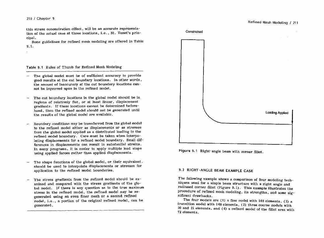
210 I Chapter 9 Refined Mesh Modeling / 211
this stress concentration effect, will be an accurate representa- tion of the actual case at those locations, i.e., St. Venet’s prin- cipal.
Some guidelines for refined mesh modeling are offered in Table 9.1.
Table 9.1 Rules of Thumb for Refined Mesh Modeling
- The global model must be of sufficient accuracy to provide good results at the cut boundary locations. In other words, the amount of inaccuracy at the cut boundary locations can- not be improved upon in the refined model.
- The cut boundary locations in the global model should be in regions of relatively flat, or at least linear, displacement gradients . If these locations cannot be determined before- hand, then the refined model should not be generated until the results of the global model are available.
- Boundary conditions may be transferred from the global model to the refined model either as displacements or as stresses from the global model applied as a distributed loading to the refined model boundary. Care must be taken when interpo- lating displacements for a refined model boundary. Small dif- ferences in displacements can result in substantial strains. In many programs, it is easier to apply multiple load steps using applied forces rather than applied displacements.
- The shape functions of the global model, or their equivalent, should be used to interpolate displacements or stresses for application to the refined model boundaries.
The stress gradients from the refined model should be ex- amined and compared with the stress gradients of the glo- bal model. If there is any question as to the true maximum stress in the refined model, the refined model may be re- generated using an even finer mesh or a second refined model, i.e., a portion of the original refined model, can be generated.
Constrained
Figure 9.1 Right-angle beam with corner fillet.
9.2 RIGHT-ANGLE BEAM EXAMPLE CASE
The following example shows a comparison of four modeling tech- niques used for a simple beam structure with a right angle and radiused corner fillet (Figure 9.1). This example illustrates the procedure of refined mesh modeling, its strengths, and some sig- nificant drawbacks.
The four models are (1) a fine model with 168 elements, (2) a transition model with 148 elements, (3) three coarse models with 20 and 21 elements, and (4) a refined model of the fillet area with 72 elements .

212 I Chapter 9 Refined Mesh Modeling / 213
Highest Density in Fillet: Point of Anticipated Maximum Stress
Figure 9.2 Right-angle beam, fine model, 168 elements.
The fine model (Figure 9.2) represents the corner fillet by using 10 rows of elements to represent the fillet radius and four layers of elements evenly spaced to pick up the stress gradient into the depth of the beam for a total of 168 elements, 203 nodes, and 392 active degrees of freedom. The computer runtime for this and the other models is given in Table 9.2. As expected, the point of maximum calculated stress was in the fillet radius, as shown in Figure 9.3. The maximum calculated stresses are given in Table 9.3.
A transition model was developed having the same grid den- sity in the fillet region, but a reduced density gridwork at the noncritical ends of the beam (Figure 9.4). The transition from
Table 9.2 Details and Computer Runtimes for Three Right-Angle Beam Models
Coarse models 20 elements (two-dimensional, plane 33 Nodes 60 active DOF Times (set)
Element formulation Wavefront solution Stress solution Element forces Misc.
Total
stress)
3.218 (0.161 sec/elem.) 1.515 1.715 (0.086 sec/elem.) 0.127 6.216
12.791 set
Transition model 148 Elements (two-dimensional, plane stress) 165 Nodes 328 active DOF Times (set)
Element formulation 23.088 (0.156 sec/elem.) Wavefront solution 8.133 Stress solution 12.318 (0.083 sec/elem.) Element forces 0.918 Misc. 20.476
Total 64.933 set
Fine model 168 Elements (two-dimensional, plane stress ) 203 Nodes 392 active DOF Times (set)
Element formulation 27.412 (0.163 sec/elem.) Wavefront solution 9.473 Stress solution 14.021 (0.083 sec/elem.) Element forces 1.042 Misc. 12.416
Total 73.742 set
Note : Computer runtimes are valid for a relative comparison be- tween models and cases.

214 I Chapter 9 Refined Mesh Modeling I 215
Maximum Principal Stress Location
Figure 9.3 Stress contour plot, fine model, maximum principal stress.
the detailed to coarse gridwork was accomplished by a pattern of triangular elements that reduce by half the number of elements per2 row. The comparison of computer runtimes shows that the transition model required 88% of the computer time of the fine model and gave comparable results, especially the maximum no- dal stresses. The difference in stresses is probably due more to using triangular elements in the model than to the difference in the number of elements. It must be noted that the transition model because of its nonuniformity requires more effort to cre- ate the model and input the data than the fine model, and it does not lend itself as easily to automatic mesh generation.
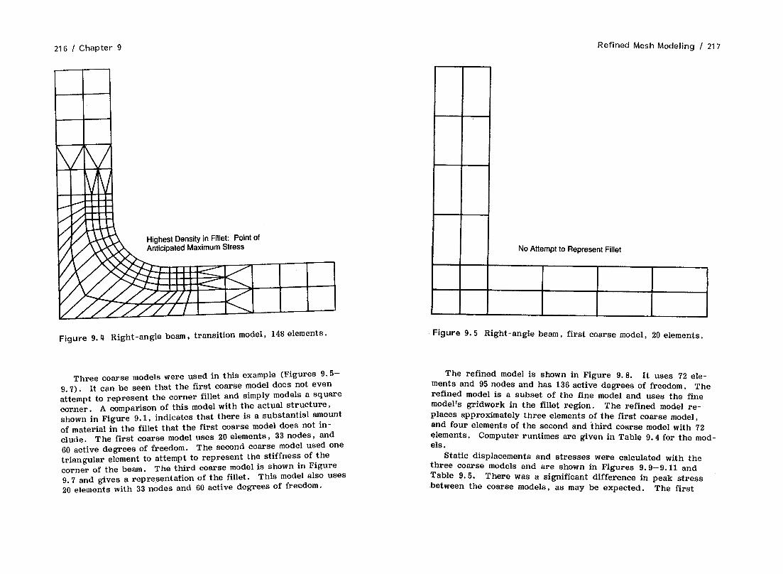
216 I Chapter 9 Refined Mesh Modeling I 217
hest Density in Fillet: Point of icipated Maximum Stress
Figure 9.4 Right-angle beam, transition model, 148 elements.
Three coarse models were used in this example (Figures 9.5- 9.7). It can be seen that the first coarse model does not even attempt to represent the corner fillet and simply models a square corner . A comparison of this model with the actual structure, shown in Figure 9.1, indicates that there is a substantial amount of material in the fillet that the first coarse model does not in- elude. The first coarse model uses 20 elements, 33 nodes, and 60 active degrees of freedom. The second coarse model used one triangular element to attempt to represent the stiffness of the corner of the beam. The third coarse model is shown in Figure 9.7 and gives a representation of the fillet. This model also uses 20 elements with 33 nodes and 60 active degrees of freedom.
No Attempt to Represent Fillet
Figure 9.5 Right-angle beam, first coarse model, 20 elements.
The refined model is shown in Figure 9.8. It uses 72 ele- ments and 95 nodes and has 136 active degrees of freedom. The refined model is a subset of the fine model and uses the fine model’s gridwork in the fillet region. The refined model re- places approximately three elements of the first coarse model, and four elements of the second and ‘third coarse model with 72 elements, Computer runtimes are given in Table 9.4 for the mod- els .
Static displacements and stresses were calculated with the three coarse models and are shown in Figures 9.9-9.11 and Table 9.5. There was a significant difference in peak stress .between the coarse models, as may be expected. The first

218 I Chapter 9 Refined Mesh Modeling I 219
\
Fillet is Over-stiff With Triangular Element
Figure 9.6 Right-angle beam, second coarse model, 21 elements.
coarse model, which does not model the fillet, gave a maximum prfncipal nodal stress of 852.02. Its maximum centroidal stress was only 439.86. Due to such a few elements, the element cen- troid was only half-way between the beam surface and neutral axis. The location of the maximum stress in the first coarse model was away from the corner, on the top surface of the horl- zontal leg of the beam. The second coarse model, which differs from the first only by the addition of a triangular element to represent the fillet, had a maximum principal nodal stress of 851.44 in the same location. The third coarse model that in- cludes a fillet radius modeled with four elements had a maximum
Coarse Representation of Circular Fillet
Figure 9.7 Right-angle beam, third coarse model, 20 elements.
nodal principal stress of 842.42 in the fillet. Comparing the three maximum stress numbers from the coarse models against the maxi- mum principal node1 stress from the fine model (971.00) shows that even the third coarse model does not give results that are better than 87% of the fine model’s result. The third coarse model did, however, give the correct location of maximum prin- cipal stress.
The results of the corresponding refined models are given in Table 9.5 and Figures 9.12-9.14 based on displacements from the three coarse models. The same refined model was used for all three cases, the only difference being the applied cut

220 I Chapter 9 Refined Mesh Modeling 1 221
Replaces About Three Elements of First and Third Coarse Models; Four Elements of Second Coarse Model
Figure 9.8 Right-angle beam, refined model of fillet area, 72 ele- ments.
boundary displacements. The results showed that the displace- ments of the first coarse model, when used with the refined model, overpredicted the maximum principal stress based on the results of the fine model. This is due to the fact that the first coarse model overpredicts the displacements at the cut boundary locations because of the lack of material in the fillet and the re- sulting underprediction of stiffness in the fillet. The second coarse model’s displacements underpredict stress because they underpredict the displacements at the cut boundary locations of the coarse model. Although there was a substantial difference between the nodal stresses of the refined model with the first
Table 9.4 Details and Computer Runtimes for Right-Angle Beam Refined Model
Coarse models 20 Elements (two-dimensional, plane stress) 33 Nodes 60 active DOF Times (see)
Element formulation 3.218 (0.161 sec/elem.) Wavefront solution 1.515 Stress solution 1.715 (0.086 sec/elem.) Element forces 0.127 Misc. 6.216
Total 12.791 set
Fine model 168 Elements (two-dimensional, plane stress) 203 Nodes 392 active DOF Times (see)
Element formulation 27.412 (0.163 sec/elem.) Wavefront solution 9.473 Stress solution 14.021 (0.083 sec/elem.) Element forces 1.042 Misc. 12.416
Total 73.742 set
Refined model 72 Elements (two-dimensional, plane stress) 95 Nodes 136 active DOF Times (set)
Element formulation 11.888 (0.165 sec/elem.) Wavefront solution 3.813 Stress solution Element forces
6.124 (0.085 sec/elem.) 0.430
Misc. 13.430
Total 35.685 set
Note : Computer runtimes are valid for a relative comparison be- tween models and cases.

222 I Chapter 9 Refined Mesh Modeling / 223
Figure 9.9 First coarse model, maximum principal stress.
and second coarse model displacement, the relative stress dis- tributions are virtually identical as shown in Figures 9.12 and 9.13. Surprisingly, the results of the combination of the third coarse model with the refined model did not significantly improve the results, relative to the fine model.
Several variations were tried with the refined model to test its sensitivity to modeling variables. The first test involved in- creasing the number of elements in the refined model by adding 16 additional elements (4 rows of 4) to the “top” of the model. The purpose of this exercise is to test whether or not the cut boundary is far enough from the fillet region so as not to be influenced by the fillet. The results shown in Table 9.6 show
Stress Results Highly Inaccurate
Figure 9.10 Second coarse model, maximum principal stress.
that there is some difference in maximum centroidal stress, but virtually no difference in maximum nodal stress.
The second test was aimed at determining the effect of accu- racy of the interpolated, cut boundary displacements. Displace - ments along the top cut boundary were, intentionally, adjusted by 1% and the results are shown in Table 9.6. There was only about 0.5% difference in stresses.
The significant conclusions that can be drawn from this ex- ample case are that the coarse model has a significant influence of the end results and that a too coarse model will not give

224 I Chapter 9 Refined Mesh Modeling I 225
ess Results Will Be Low, but at Least Approximation of Actual Stress
Figure 9.11 Third coarse model, maximum principal stress.
accurate results, regardless of how detailed the refined model is. The use of the first coarse model with no representation of the fillet radius was selected as a limiting case to determine the ef- fect of using an extremely coarse model. The lack of material in the fillet caused the first coarse model to have displacements that were too high at the locations of the cut boundaries of the refined model. When these displacements were transferred from the coarse model to the boundaries of the refined model, the re- sult was high stress in the refined model. In the case of this

226 I Chapter 9 Refined Mesh Modeling I 227
aximum Principal Stress Location
Figure 9.12 Refined model, maximum principal stress: First coarse model displacements.
right angle beam, the details of the fillet geometry are not insig- nifieant and need to be accurately included in the coarse model.
9.3 REFINED MODELING: EXAMPLE CASES
Several of the simple example cases of Chapter 5 will be used again to demonstrate the application of refined mesh modeling. Not all of the examples were chosen to show the positive side of this technique. Some of the example cases will show that
Maximum Principal Stress Location
Figure 9.13 Refined model, maximum principal stress: Second coarse model displacements.
refined mesh modeling should be selectively applied and is not the universal solution to obtaining optimum accuracy.
9.3.1 Example: Notched Block
The notched block two-dimensional model from Chapter 5, Section 5.4.2 is used here to illustrate the principals and procedures of refined mesh modeling. The two-dimensional global model is shown in Figure 9.15. This model has 38 two-dimensional plane strain elements, 49 nodes, and 82 active degrees of freedom. The global model uses 12 elements to represent the fillet area. This example, like the L-shaped beam, shows the gains in accuracy

228 I Chapter 9 Refined Mesh Modeling I 229
Maximum Principal Stress Location
Figure 9.14 Refined model, maximum principal stress: Third coarse model displacements.
of refined mesh modeling, but also points out the price in terms of computer and modeling time.
The refined model is shown in Figure 9.16 and has a total of 64 elements, 166 nodes, and 280 active degrees of freedom. The area of the refined model is approximately eight elements of the global model. Computer runtimes for both models are given in Table 9.7. As expected, the computer time for the refined model was about double that of the global model because of the number of elements and degrees of freedom in each.

230 I Chapter 9
Figure 9.15 Notched block, two-dimensional global model.
The stress results presented in Table 9.8 showed that there .was a moderate difference in the results between the global model and the refined model. The refined model gave higher stresses for the Y direction (the direction of load) and the max- imum principal stress. A plot of the refined stress distribu- tion is shown in Figure 9.17.
Refined Mesh Modeling I 231
Nodes
Figure 9.16 Notched block, two-dimensional refined model.
In this case, the global model was not only sufficiently accu- rate, but it would appear that the use of a refined model with twice the number of elements and twice the computer runtime is hard to justify. A more cost-effective approach to this model might be to simply increase the number of elements in the fillet area to achieve a slightly better resolution of the stress field.
9.3.2 Example : Crank
The crank, discussed in Chapter 5, Section 5.4.4 and shown in Figure 9.18, represents a more practical application of refined

232 I Chapter 9
Table 9.7 Details and Computer Runtimes for Block Refined Model
Refined Mesh Modeling / 233
Table 9.8 Stress Results of Notched Block Refined Model
Two-dimensional global model 38 Elements (two-dimensional, plane strain) 49 Nodes 82 active DOF Times (set)
Element formulation 8.149 (0.214 seclelem.) Wavefront solution 2.158 Stress solution 2.515 (0.066 sec/elem.) Element forces 0.276 Misc. 3.510
Total 16.600 set
Two-dimensional block refined model 64 Elements (two-dimensional, plane strain) 165 Nodes 280 active DOF Times (see)
Element formulation 11.788 (0.184 sec/elem.) W avefront solution 3.491 Stress solution 5.412 (0.303 sec/elem.) Element forces 0.406 Misc. 12.63
Total 33.73 set
Note : Computer runtimes are valid for a relative comparison be- tween models and cases.
mesh modeling in the keyway area. In the global model, three elements are used to bound the keyway and there is no attempt to model the stress field in the corner of the keyway. In the global model, the key is not explicitly included in the model; the nodes on the keyway that would contact the key are constrained in the tangential direction to simulate the effect of the key bear- ing on the keyway.
A three-dimensional refined mesh model of the keyway region is developed and shown in Figure 9.19. The refined model con- tains 168 three-dimensional solid elements (the same element used
Maximum centroidal stress Maximum nodal stress
OX aY 07. 01 *X (5 02 01
Two-dimensional global model
3.24 8.70 3.58 8.86 3.40 12.68 4.82 13.50
Two-dimensional refined model
3.06 6.45 2.86 8.38 1.24 14.11 4.61 14.27
OX = X direction stress 9 = Y direction stress TXZ = shear stress 01 = maximum principal stress
in the global model), 241 nodes, and 720 active degrees of free- dom . The refined model uses 14 elements per layer to bound the keyway and positions one element at each corner to represent a small chamfer, which would normally occur in practice as the keyway is either broached or shaped.
The refined model had a free surface that was the inside of the keyway and three cut surfaces on the outside boundaries. There was one additional free surface of the refined model cor- responding to the top of the crank and one additional cut sur- face at the “bottom” of the refined model. Three displacements were interpolated from the global model for each of the refined cut boundary nodes.
Computer runtimes are given in Table 9.8. Although the ratio of the number of elements between the two models was 1.33~1 and the ratio of the number of active degrees of freedom was 1.81:1, the ratio of total runtimes was 2.32:1. This is due to the de- creased time for the frontal equation solution of the refined model that, in turn, is due to the more efficient element numbering, 1.e. , smaller wavefront, of the refined model.

234 I Chapter 9 Refined Mesh Modeling I 235
Figure 9.17 Notched block, two-dimensional refined model, max- imum principal stress.
Figure 9.18 Crank, three-dimensional global model.
3D Refined Model 01 Section of Keyway
Figure 9.19 Crank, three-dimensional refined model of keyway.
The maximum principal stresses and the component stresses at the keyway are presented in Table 9.10. The comparison of maximum principal stresses shows that there is a 43% difference between the maximum centroidal stresses of the two models that is to be expected because the global model defines the keyway with a minimal three elements per layer and the refined model uses 14 elements per layer. Furthermore, the centroid of the refined model is much closer to the surface of the keyway than the centroid of the global model.
There was a smaller, 28% difference between the maximum principal node1 stresses of the two models, indicating that

236 I Chapter 9 Refined Mesh Modeling I 237
Table 9.9 Details and Computer Runtimes for Crank Refined Model Table 9.10 Stress Results of Crank Model
Three-dimensional global model 224 Elements (three-dimensional, solid) 459 Nodes 1306 active DOF Times (see)
Element formulation 320.53 (1.431 seclelem.) Wavefront solution 427.95 Stress solution 77.609 (0.346 sec/elem.) Element forces 5.821
37.418
Total 924.38 set
Three-dimensional refined model 168 Elements (three-dimensional, solid) 241 Nodes 720 active DOF Times (see)
Element formulation 142.55 (0.849 sec/elem.) W avefront solution 156.25 Stress solution 43.379 (0.258 seclelem.) Element forces 3.161 Misc. 44.580
Total 398.92 set
Note : Computer runtimes are valid for a relative comparison be- tween models and cases.
although the global model elements did a fair job extrapolating stresses to the node points, there is a limit to how much extrap- olation these LDADS elements are capable of. The differences between the centroidal and nodal stresses of the two elements in- dicate that the LDADS elements are capable of estimating a stress gradient. The refined model, with its smaller elements, shows a smaller (0.9% compared to 13.2%) difference between the maximum centroidal stress and the maximum nodal stress.
A stress contour plot of the maximum principal stress in the global model around the keyway is shown in Figure 9.20 and a maximum principal stress plot for the refined model is shown in Figure 9.21.
Maximum centroidal stress
or Ot ‘a Ol
Maximum nodal stress
ar "t oa 01
Global model, keyway
-371.38 785.90 66.87 1126.8 -497.71 943.36 142.53 1274.43
Refined model, keyway
68.27 1606.3 284.11 1615.3 -109.63 491.14 4.53 1630.22
or = radial (relative to shaft bore) stress at keyway at = tangential stress at keyway oa = axial stress at keyway ur = maximum principal stress at keyway
Highly Inaccurate
Figure 9.20 Crank, global nodal keyway area, maximum principal stress.

238 I Chapter 9 Refined Mesh Modeling I 239
Reasonable Maximum St1
Figure 9.21 Crank, refined model keyway area, maximum prin- cipal stress.
In addition to calculating the maximum stresses, the refined model is necessary, in this case, to achieve any sort of reason- able definition of the stress field away from the surface of the keyway. This stress field definition would be necessary in cases of localized plasticity in the corners of the keyway or for fracture mechanics’ applications for predicting crack growth.
9.3.3 Example: Gear Segment
A refined model of the fillet of the two-dimensional single gear tooth model, described in Chapter 5, Section 5.4. 5. The global,
Reasonable Definition of Fillet High Stress Gradients Require Additional Elements
Figure 9.22 Single gear tooth, two-dimensional global model.
Shape
two-dimensional single tooth model is shown in Figure 9.22 and the refined model is shown in Figure 9.23. The area of the re- fined model covers five elements of the global model. The re- fined model has 60 elements, 80 nodes, and 112 active degrees of freedom, virtually the same numbers as the global model. The free surface of the refined model includes the fillet radius and transition to the involute curve. The refined model has three cut surfaces for which the nodal displacements were interpolated from the global model results.
The computer runtimes are shown in Table 9.11. As expected, the runtimes for the global model and refined model were very
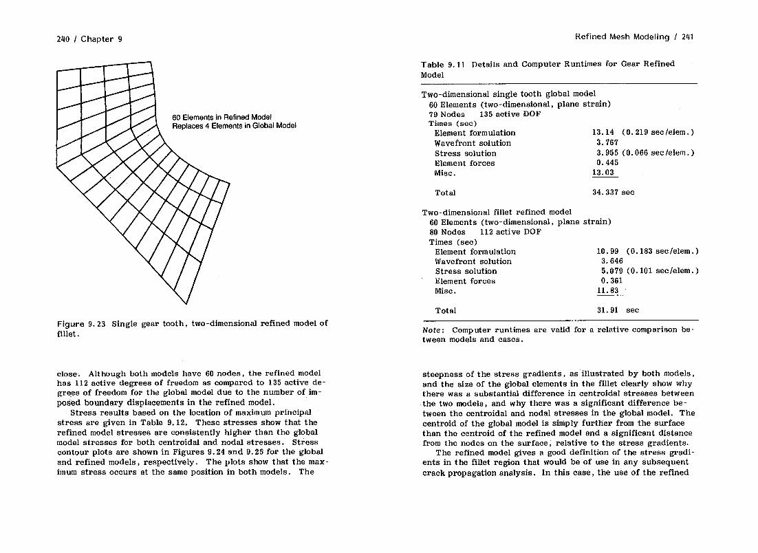
240 I Chapter 9 Refined Mesh Modeling / 241
60 Elements in Refined Model Replaces 4 Elements in Global Model
Figure 9.23 Single gear tooth, two-dimensional refined model of fillet.
close. Although both models have 60 nodes, the refined model has 112 active degrees of freedom as compared to 135 active de- grees of freedom for the global model due to the number of im- posed boundary displacements in the refined model.
Stress results based on the location of maximum principal stress are given in Table 9.12. These stresses show that the refined model stresses are consistently higher than the global model stresses for both centroidal and nodal stresses. Stress contour plots are shown in Figures 9.24 and 9.25 for the global and refined models, respectively. The plots show that the max- imum stress occurs at the same position in both models. The
Table 9.11 Details and Computer Runtimes for Gear Refined Model
Two-dimensional single tooth global model 60 Elements (two-dimensional, plane strain) 79 Nodes 135 active DOF Times (set)
Element formulation 13.14 (0.219 sec/elem.) Wavefront solution 3. ‘76’7 Stress solution 3.955 (0.066 sec/elem.) Element forces 0.445 Misc. 13.03
Total 34.337 set
Two-dimensional fillet refined model 60 Elements (two-dimensional, plane strain) 80 Nodes 112 active DOF Times (set)
Element formulation 10.99 (0.183 sec/elem.) Wavefront solution 3.646 Stress solution 5.079 (0.101 sec/elem.) Element forces 0.361 Misc. 11.83
Total 31.91 set
Note: Computer runtimes are valid for a relative comparison be- tween models and cases.
steepness of the stress gradients, as illustrated by both models, and the size of the global elements in the fillet clearly show why there was a substantial difference in centroidal stresses between the two models, and why there was a significant difference be- tween the centroidal and nodal stresses in the global model. The centroid of the global model is simply further from the surface than the centroid of the refined model and a significant distance from the nodes on the surface, relative to the stress gradients.
The refined model gives a good definition of the stress gradi- ents in the fillet region that would be of use in any subsequent crack propagation analysis. In this case, the use of the refined

242 I Chapter 9
Table 9.12 Stress Results of Gear Refined Model
Maximum centroidal stress Maximum nodal stress
or oa (2 (Jl % Oa at Dl
Two-dimensional single tooth global model, plane strain
506.7 228.4 254.4 588.0 904.3 382.8 371.8 1063.2
Two-dimensional filled refined model, plane strain
868.55 341.66 270.33 1009.2 1157.22 439.48 307.71 1347.3
u r = radial stress aa = axial stress at = tangential stress o1 = maximum principal stress
model allowed for a good determination of maximum stress and stress gradients in the critical region of the gear tooth in a cost- effective manner. Using the same element density in the global model as the refined model would require 12 times the number of elements in the global model. Even by developing a transition model, using a fine gridwork in the fillet with a transition to a coarse gridwork, elsewhere, would require considerably more modeling effort and still require almost an order of magnitude more elements.
9.3.4 Example : Turbine Blade
In this example, following the three-dimensional model described in Chapter 5, Section 5.4.6, a two-dimensional plane strain, re- fined model is used in conjunction with the three-dimensional glo- bal model. As discussed in Chapters 4 and 5, the turbine blade is attached to the turbine rotor via a firtree root attachment de- sign as shown in Figure 9.26. Although this attachment area is modeled with 440 (five layers of 88) three-dimensional elements, the definition of the fillets is marginal, at best, as shown in Fig- ure 9.27.
The refined two-dimensional model uses 832 elements to model the two-dimensional blade attachment and rotor segment, as
Refined Mesh Modeling / 243
Note: Maximum Stress Location Away From Fillet and Close to Cut Boundary. High Stresses Occurring Close to a Cut Boundary Are Always Suspect.
Figure 9.24 Single gear tooth, two-dimensional global model, maximum principal stress.
shown in Figures 9.28 and 9.29. This gives almost 10 times the number of elements in the two-dimensional model as there are in one three-dimensional layer. There are 428 elements used to model the blade root and 404 elements used to model the rotor segment that has approximately the same proportions as the three-dimensional rotor segment. The use of the two-dimen- sional model allows gap elements to be used at the contacting surfaces. The gap elements allow for friction effects to be in- cluded in the model and for the effects of incomplete initial con- tact between all six load-bearing surfaces to be investigated. In other words, a situation could arise in which one or more of the

244 I Chapter 9
Maximum Stress Location in Fillet as Expected
Figure 9.25 Single gear tooth, two-dimensional refined model, maximum principal stress.
“hooks” were not initially in contact. The remaining hook would be more heavily loaded and therefore more highly stressed. The use of gap elements allows for an initial open gap to be specified and included in the calculation.
The computer runtimes are given in Table 9.13. The three- dimensional global model is described in Chapter 5 and uses 735 three-dimensional solid elements. The two-dimensional, refined model includes gap elements that require an iterative solution. Substructuring was used to reduce down the problem size to only the degrees of freedom connected to the gap elements, Back sub- stitution for stresses was carried out for the blade root only. Sub- structuring will be discussed in more detail in Chapter 10.
Rotor Segment Removed for Clarity Highest Stress in Fillet as Expected Each Fillet Modeled With Only 3 Elements
Figure 9.26 Turbine blade firtree root attachment, three-dimen- sional model.
Both Blade and Rotor Segment Shown. Each Fillet Modeled With Only 3 Elements Along Profile by One Layer of Elements Into Depth.
Figure 9.27 Turbine blade firtree root attachment, model profile.

246 / Chapter 9 Refined Mesh Modeling I 247
20 Refined Model has Problem of Approximating 30 Stress Field With 20 Plane Stress Calculation
Figure 9.28 Turbine blade root attachment, two-dimensional re- fined model.
The maximum principal stress occurred in the upper hook fillet as shown in Figure 9.30. A comparison of stresses is given in Table 9.14. The calculated elastic stress for the refined model exceeded the yield strength of the material, indicating that there should be some localized plastic deformation in the hook fillet. A direct comparison of stresses is not valid here, because the glo- bal model is a full three-dimensional model, whereas the refined model is a two-dimensional plane strain model. The main purpose of the refined model in this case is to form a comparison of radial
Three Elements in 30 Global Model Replaced by 33 2D Elements in Refined Model
Figure 9.29 Turbine blade root attachment, two-dimensional re- fined model, blade only.
and tangential component stresses. The radial stress is the pre- dominant stress and contributes the most to the maximum princi- pal stress. This comparison shows that the maximum stresses are fairly close. Both the maximum centroidal and nodal stress- es for the three-dimensional global model were higher than the corresponding two-dimensional refined stresses. It must be as- sumed, however, that the stress distribution into the depth of the part should be more accurate with the refined model.
9.4 PLATE-SOLID TRANSITIONS
One particular refined modeling problem that requires considera- tion is the use of a two or three-dimensional refined model with

248 I Chapter 9 Refined Mesh Modeling I 249
Table 9.13 Details and Computer Runtimes for Turbine Blade Refined Model
Three-dimensional turbine blade global model 774 Elements (three-dimensional, solid) 79 Nodes 135 active DOP Times (see)
Element formulation 692.0 (0.894 sec/elem.) Wavefront solution 2861.0 Stress solution 1018.0 (1.315 sec/elem.)
Total 4571.0 set
Two-dimensional refined root model 832 Elements (two-dimensional, plane strain) 1477 Nodes 4411 active DOF Times (set)
Element formulation 126.46 (0.152 sec/elem.) Wavefront solution 68.867
(substructure generation) Gap iteration routine 45.994 Stress solution (428 elem . ) 77.710 (0.101 sec/elem.)
Total 319.03 set
Note : Computer runtimes are valid for a relative comparison be- tween models and cases.
plate and /or beam and solid global model. Because the plate and beam elements can niodel rotations and moments which the two- and three-dimensional solid elements cannot, the application of moment must be added to the refined model with care.
:A typical instance in which this might occur is in a plate to solid transition where plate (or beam) elements are joined to solid elements. The suggested method of accomplishing this interface and transmitting the moment from the plate elements to the solid elements is to “bury” the plate elements one layer deep in the solid elements as shown in Figure 9.31. It is recommended that the plate element that is buried in the solid element have a re- duced thickness and moment of inertia because that portion of
Maximum Principal Stress Location
Figure 9.30 Turbine blade, refined two-dimensional root model, maximum principal stress.
the model will be overstiff. A rule of thumb to use in reducing the stiffness is to make those elements one-tenth the thickness and stiffness of the actual plates. In this way, the degree of overstiffness will not be too severe and any numerical problems associated with large differences in stiffness within the model will be avoided.
In forming the refined model, the translation displacements from the plate elements may be applied directly to the cut bound- ary of the refined model. The rotation or slope of the plate nodes must also be used to adjust the displacements of the re- fined model node and pivot about the center of the section. This technique is illustrated in Figure 9.32.

250 I Chapter 9 Refined Mesh Modeling I 251
n This Part of Structure too thin for 2D elements.
2D
t dx -
13 e I Plate element buried one level within 2D
- elements to provide
- moment restraint.
Notes: l Mass of “Buried” Beam Element should be zero.
l Stiffness of “Buried” Beam Element should be l/l 0 of other Beam Elements.
Figure 9.31 Plate-to-solid transition modeling.

252 I Chapter 9 Refined Mesh Modeling / 253
Plate Elements Force and Moments Transmitted at
,I Each Node
Force and Moment Resolved into Equivalent Force Distribution
Solid Refined Model
9.5 THERMAL EFFECTS
When thermal effects are included in the global model, it is im- perative that they be transferred to the refined model. This is necessary because the displacements of the global model are a combination of thermal expansion and deformation due to applied loading. The cut boundary displacements are, therefore, also a combination of these two effects. If the refined model does not have the correct nodal temperatures applied to all nodes and is allowed to expand (or contract) to the same extent as the global model, then the refined model internal displacements will not be consistent with the cut boundary applied displacements.
An example is a global model in which thermal expansion and deformation due to applied loadings are of the same magnitude. If cut boundary displacements are applied to the boundary of the refined model and stresses are calculated at room temperature, i.e. , no internal thermal expansion, then the stresses will be much higher than they actually are because the model will be “pulled” from the boundaries to the full amount of the combined displacements.
9.6 SUMMARY
Refined mesh modeling represents a cost-effective means of mod- eling large, complex structures with small details that can give local stress concentrations. Although the examples shown here are rather simple, actual applications to structures such as pres- sure vessels with valve and nozzle attachments or large machinery models with bolted joints represent opportunities to achieve better accuracy with moderate cost.
REFERENCE
1. Peterson, R. E., Stress Concentration Factors, Wiley, New York, 1974.
Figure 9.32 Use of plate element displacements with solid refined models.

10
SUBSTRUCIIIRING
Many finite element models feature repetitive geometry. In prob- lems such as gear teeth or groups of turbine blades, it may be necessary to represent a repeated component in a model. Repeti- tive geometry can be efficiently modeled by the use of substruc- turing. A substructure is a finite-element model for which the internal degrees of freedom have been solved for in terms of the boundary degrees of freedom (Figure 10.1). This reduced model can then be used as an element, even though it represents a com- plex geometry, and connected to other substructures or individ- ual elements within a global model. In some finite element codes, a substructure is also known as a superelement. The terms may or may not be synonymous, depending on the system. The user must take care to consult the code documentation to determine the exact definition when those terms are used.
10.1 SUBSTRUCTURING PROCEDURES
Substructuring is performed when a repetitive geometry would re- quire generation and solution of identical sets of element stiffness
255

256 I Chapter 10 Substructuring I 257
Substructure Model Before Condensation
Internal DOF are Removed
Boundary DOF are Retained for Coupling with Other Substructures
Substructure Model After Condensation
Figure 10.1 Generalized substructure.
matrices. The mathematics of substructuring are discussed in Chapter 2, Section 2.11. In short, the individual element stiff- nes matrices (and mass matrices, if appropriate) are assembled as in a static solution and the matrix reduction process is be- gun. However, rather than completing the solution procedure to obtain an explicit solution, the set of matrix equations is
only partially solved to provide a condensed set of equations, i.e., the substructure, and a back-substitution matrix that can provide the displacement solution once the retained or master degrees-of-freedom displacements are obtained.
In order to use substructuring, the user must understand the procedures involved. Although substructuring is aimed at maximidng the efficiency of computations, there is a price to be paid in terms of modeling and bookkeeping effort. An analysis using substructures must be performed in several steps.
1. Layout of the global model and identification of areas to be substructured. Layout and development of the substructure model. Identification of boundary nodes to be retained in the substructure.
2. Generation and condensation of the substructure stiffness matrix. This is the substructure generation pass.
3. Generation of the global model by using the reduced sub- structure as many times as required and combining it with other substructures and individual elements. The solution of the glo- bal model gives the displacements at the retained, boundary de- grees of freedom of the substructures. This is the use pass.
4. Back-substitution of the boundary displacements into the original substructure model to obtain all displacements and stress- es within the substructure. This step may be repeated as many times as necessary because when a substructure is repeated with- in a global model, there will be different sets of boundary dis- placements each time the substructure is repeated in a different location in the global model.
10.2 PRACTICAL CONSIDERATIONS
Some rules of thumb governing the use of substructuring are given in Table 10.1. Care must be taken in the application of boundary conditions in a model where substructures are used. Displacement constraints may be applied in the substructure gen- eration pass or in the global, substructure use pass. If a node is constrained in the substructure generation pass, however, it will be constrained in all subsequent runs using the substruc- ture. It is not possible to unconstrain a node in a subsequent substructure use pass if it has been constrained in the genera- tion pass because the specified degrees of freedom have been re- moved. In the event that a particular degree of freedom is to be constrained in one “copy” of a repeated substructure and not in

258 I Chapter 10 Substructuring / 259
Table 10.1 Rules for Substructuring
1.
2.
3.
4.
5.
A substructure may be generated from individual elements, other substructures, or both.
Master nodes to be retained must be identified and specified in the input to the substructure generation run. Master nodes consist of boundary nodes that must be retained for connection with the rest of the global model and nodes for applied forces.
Nodal constraints specified in the substructure generation step will be constrained in all subsequent uses of the sub- structure and can never be released. Nodal constraints may, however, be applied in the global model to substructure mas- ter nodes.
Along a substructure boundary that will be used for connec- tion to the rest of the global model, all nodes must be re- tained as master nodes.
To be cost-effective, a substructure must be used three times. If a portion of a model is repeated only once, i.e. , appears twice in the structure, then substructuring will probably not be cost-effective in terms of computer runtime, not to mention the additional modeling and analysis labor time.
another copy, then that degree of freedom should be retained as a master in the substructure generation pass and later constrained in the use pass.
Substructuring can be a very cost-effective way of handling repetitive geometries; however, there is an overhead cost in com- puter time and storage. A good rule of thumb is to have a need to repeat part of a structure two times, for a total of three copies, to make substructuring cost-effective. If a part of a structure is repeated only once, i .e . , appears in the structure only twice, then substructuring probably should not be used. There is a considerable amount of additional modeling and bookkeeping ef- fort required in substructured models not required in other cases. In short, the use of substructuring is a tradeoff between com- puter time savings and additional labor time.
There are several other situations in which substructuring may be used. When several different structures contain the same component, it may be cost-effective to form a substructure of that component and archive the substructure so that it may be used in different models and analyses.
Another reason for substructuring is for models that are sim- ply too large to fit into the computer as a single model. In these events, the initial model may be broken down into a collection of substructures that, in turn, may be reduced to their boundary nodes, assembled together into a global model, solved for the mas- ter degrees of freedom, and the individual substructures may be back-substituted for stresses. For a large model, substructuring will not be as cost-effective as solving the problem as a single large model; however, it does represent an alternative to an im- possible model.
A third reason for substructuring exists when nonlinear prob- lems are involved, such as gap elements that require an iterative solution. In such cases, the linear portion of the model can be generated as a substructure and reduced down to a selected set of master degrees of freedom. The nonlinear elements can be solved iteratively and the final stress solution may be obtained by back-substitution.
10.3 EXAMPLE: CIRCULAR PLATE
In cases where one substructure is generated and repeated sev- eral times within a global model, the stresses within the sub- structure copies will not be the same but vary depending on the location of the substructure copy within the global model. As an example, a circular plate is shown in Figure 10.2. An un- substructured model of the plate is shown in Figure 10.3. It is easy to see that due to the symmetric nature of the geometry, there is substantial repetition of the elements. However, due to the nonsymmetric loading at the center hole, the model can- not be made smaller by using symmetry. The 10 bolt holes in the plate for fastening require a substantial number of elements to correctly represent the geometry and give a reasonable cal- culation of stress in those areas.
A substructure of one segment of the plate is shown in Fig- ure 10.4. This substructure represents one-tenth of the plate (36”). Because the bolt holes are evenly spaced, it is possible to form one substructure and repeat it 10 times to form a plate model.

260 1 Chapter 10
Bolt Holes Completely Constrained Forces Applied at Center Hole
I
Substructuring I 261
Forces Applied to Nodes at Center Hole All DOF at Bolt Holes Constrained to Zero
230
Figure 10.3 Circular plate unsubstructured model.
Asymmetric Pattern of Forces Makes it impossible to Use Symmetry to Reduce Problem Size
Figure 10.2 Circular plate substructuring example.
An unsubstructured model contains 230 elements and 260 nodes (520 DOF) as shown in Figure 10.3. The substructure contains 23 elements and 33 nodes that are reduced down to 14 master nodes at the symmetric boundaries. Displacement constraints
are applied at the bolt hole in the substructure generation run so that those degrees of freedom are “permanently” constrained and no additional displacement constraints need to be specified in the subsequent use runs. The global model, consisting of 10 copies of the substructure, contains only 70 unique master nodes (140 DOF).
Forces are applied at the center of the plate in the substruc- ture use run at the boundary nodes so that additional nodes do not need to be retained for the application‘of forces. The as- sembly of substructures is shown schematically in Figure 10.5.
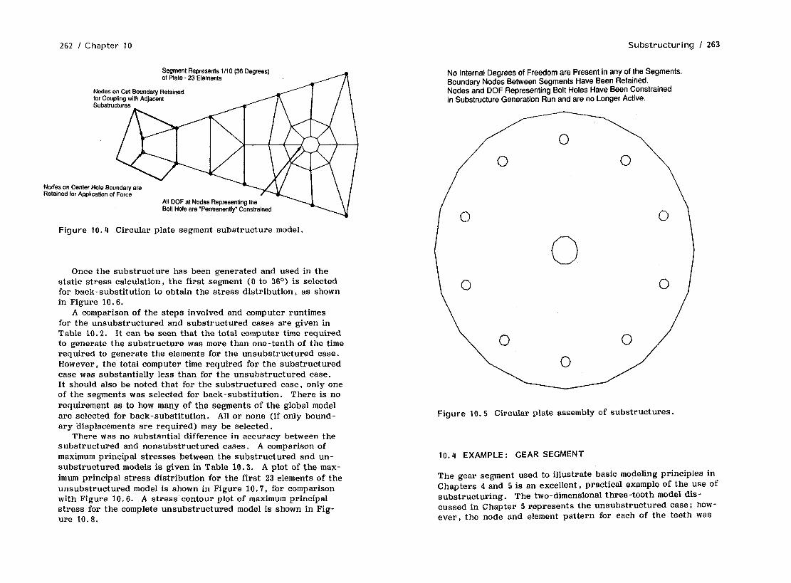
262 / Chapter 10 Substructuring I 263
Segment Represents 1110 (36 Degrees) of Plate - 23 Elements
Nodes on Cut Boundary Retained for Coupling with Adjacent
Nodes on Center Hole Boundary are Retained for Application of Force
All DOF at Nodes Representtng the Bolt Hole are “Permanently” Constrained
Figure 10.4 Circular plate segment substructure model.
Once the substructure has been generated and used in the static stress calculation, the first segment (0 to 369 is selected for back-substitution to obtain the stress distribution, as shown in Figure 10.6.
A comparison of the steps involved and computer runtimes for the unsubstructured and substructured cases are given in Table 10.2. It can be seen that the total computer time required to generate the substructure was more than one-tenth of the time required to generate the elements for the unsubstructured case. However, the total computer time required for the substructured case was substantially less than for the unsubstructured case. It should also be noted that for the substructured case, only one of the segments was selected for back-substitution. There is no requirement as to how many of the segments of the global model are selected for back-substitution. All or none (if only bound- ary ?lisplacements are required) may be selected.
There was no substantial difference in accuracy between the substructured and nonsubstructured cases. A comparison of maximum principal stresses between the substructured and un- substructured models is given in Table 10.3. A plot of the max- imum principal stress distribution for the first 23 elements of the unsubstructured model is shown in Figure 10.7, for comparison with Figure 10.6. A stress contour plot of ,maximum principal stress for the complete unsubstructured model is shown in Fig- ure 10.8.
No Internal Degrees of Freedom are Present in any of the Segments. Boundary Nodes Between Segments Have Been Retained. Nodes and DOF Representing Bolt Holes Have Been Constrained in Substructure Generation Run and are no Longer Active.
0 0
0
Figure 10.5 Circular plate assembly of substructures.
10.4 EXAMPLE : GEAR SEGMENT
The gear segment used to illustrate basic modeling principles in Chapters 4 and 5 is an excellent, practical example of the use of substructuring. The two-dimensional three-tooth model dis- cussed in Chapter 5 represents the unsubstructured case; how- ever, the node and element pattern for each of the teeth was

264 / Chapter 10 Substructuring / 265
Maximum Principal Stress
Figure 10.6 Circular plate stress results: First segment of sub- structured model.
identical. Due to the unequal loading between the teeth, which is a function of the gear’s instantaneous angular position rela- tive to its mating gear, the stress pattern in all three teeth will not be the same. In addition, the bending of one tooth causes a compressive stress in the fillet of the next tooth that cannot be modeled with a single tooth model. For these reasons, the three-tooth model gives a more accurate representation of the fillet bending stresses than does the single tooth model.
The generation of three sets of identical stiffness matrices and their solution is, however, inefficient. The problem can be-solved to give, for all practical purposes, identical results with a savings in computer runtime by the use of substructuring. Figure 10.9 shows the unsubstructured model from Chapter 5 with 180 elements. Figure 10.10 shows the single-tooth sub- structure with 60 elements and indicating those nodes that will be retained in the substructure. The nodes to be retained are those that are necessary for joining the substructures together along their cut boundaries and those nodes necessary for apply- ing forces. It must be noted that all of the nodes on the profile

266 / Chapter 10 Substructuring ! 267
Table 10.3 Stress Results of Circular Plate: Substructured and Nonsubstructured Models
Substructured model, first segment
Maximum centroidal stress
UX UY ‘XY 01
- 124.44 47.23 -19.33 50.001
Unsubstructured model, first segment
-124.04 47.64 -19.78 49.889
(JX = X direction (horizontal axis) stress
uY = Y direction (vertical axis) stress
‘XY = shear stress 01 = maximum principal stress
Figure 10.7 Circular plate unsubstructured case, first 23 ele- ments.
Figure 10.8 Circular plate unsubstructured case: Complete plate.
to which forces will be applied are required on every tooth; how- ever, it is necessary to retain any node that will be required later as a location for applied forces. Figure 10.11 shows the condensed substructure schematically and the assembly of sub- structures. Figure 10.11 does depict the gear tooth divided into elements although at this point, after the condensation pro- cess , the internal degrees of freedom have been removed. The resulting stiffness matrix represents the relative stiffness be- tween the remaining boundary degrees of freedom. In effect, the resulting substructure is a gear tooth “element .‘I

268 I Chapter 10
Distributed Loading Resolved into Component Nodal Forces
Roller Constraints Along Cut Boundaries Segment Model Will Allow for Compressive Stress Effects to Be Calculated 180 2D Plane Strain Elements Same Mesh Pattern as Single Tooth Model But Repeated to Form Segment
Figure 10.9 Three-tooth gear segment: Two-dimensional model.
Table 10.4 gives a comparison of the computer runtimes for the substructured and unsubstructured three-tooth models. Table 10.4 shows that for the three-tooth model, which by the rule of thumb in Table 10.1 represents the minimum number of repeated structures necessary for a breakeven point, the sub- structured model required 63% of the total computer runtime of the unsubstructured case. The substructured case, it must be noted, only obtained stresses for one of the three gear teeth. This is, however, a practical situation because it may not be necessary to calculate stress in all the teeth. It should be ob- vious from the loading pattern which tooth is going to be the most highly stressed. If it is not intuitively obvious, then an examination of the displacements from the use pass may give some direction. In any event, even if stresses were calculated in all three teeth, then an estimate for the total runtime for the substructured case would be about 91% of the total time for the unsubstructured case.
A closer examination of the computer runtimes in Table 10.4 points out, for the substructured case, the relative computer time for the various phases. A linear extrapolation of times for the use pass could be used to obtain ball-park time estimates for
Boundary Nodes Retained for Coupling
Substructuring 1 269 Substructuring I 269
Boundary Nodes Retained Boundary Nodes Retained for Applied Forces for Applied Forces
I I
Boundary Nodes Retained Boundary Nodes Retained for Coupling for Coupling
Figure 10.10 Single gear tooth two-dimensional substructure model.
other numbers of gear teeth in the segment. A comparison of the relative and total runtimes shows why three repeated struc- tures are necessary to make it cost-effective to use substruc- turing. Stresses for the substructured and unsubstructured cases were virtually identical.

270 I Chapter 10 Substructuring I 271
Boundary Nodes Retained for Applied Forces
Boundary Nodes Retained Boundary Nodes Retained for Coupling for Coupling
Figure 10.11 Gear segment assembly of substructures.
10.5 TURBINE BLADE ATTACHMENT : REFINED MODEL
The turbine blade refined model from Chapter 9, Section 9.3.4 is an example of the use of substructuring to cut down on the computer time required for a nonlinear calculation. This two- dimensional plane strain model is shown in Figure 10.12. The model consists of a blade root section with 428 elements, a seg- ment of the mating turbine rotor with 405 elements, and 18 two- dimensional gap elements to represent the contact between the blade and rotor load-bearing surfaces. The use of the gap ele- ments makes the problem geometrically nonlinear and the gap elements require an iterative solution. The gap elements are allowed to be open or closed and to slide sideways. Equilibrium is achieved when all gap elements find their position, either open or closed, and there is no further sliding. This typically re- quires between 5 and 10 iterations for this type of model. In this case, substructuring is used to reduce down the initial mod- els to only those nodes that define the gap elements and those

272 I Chapter 10 Substructuring I 273
Figure IO. 12 Turbine blade attachment : Refined two-dimensional model.
nodes on the blade root to which forces are applied. Nodes to which displacement constraints are applied on the rotor segment are constrained in the generation pass.
Figure 10.13 shows schematically the final blade root and ro- tor segment substructures assembled together with the gap ele- ments. This example case differs from the previous two in that this case combines two different substructures together with conventional elements in the use pass. Figure 10.14 shows the resulting two-dimensional maximum principal stress distribution in the blade attachment portion.
Table 10.5 shows the breakdown of computer runtime for the entire analysis. It shows that the time for the gap element iter- ations was only 32 set for five iterations, a little over 6 set per iteration. This should be contrasted with the time for the
Boundary Nodes Retained for Coupling
,&, Constraints Applied to Boundary of Assembled Substructures
t Forces Applied Boundary of Assembled Substructures
Figure 10.13 Turbine blade attachment: Assembly of substruc- tures.
substructure condensation, 461.02 set, which would be roughly the same as the time to solve for all of the elements at each ite?- ation if substructuring were not used.
Chapter 9, Section 9.3.4 gives the remaining details of stress- es and comparison with the global three-dimensional model. The purpose of the discussion here is to point out another example of substructuring to minimize the computer runtime for a nonlinear problem.
10.6 SUMMARY
Substructuring does not change the overall accuracy of the anal- ysis, nor does it represent an approximation or require any

274 / Chapter 10 Substructuring / 275
Figure 10.14 Turbine blade attachment: Two-dimensional stress distribution.
additional modeling assumptions. It is merely a method of re- ducing computer runtime for repetitious structures, complex structures, or structures with limited nonlinear effects. The drawback to substructuring is that it requires more of the an- alyst’s time in setting up the models and in bookkeeping dur- ing the calculation process. Substructuring is, at a minimum, a three-step procedure even for a linear static analysis. Files must be kept track of and archived. The opportunitites for using substructuring are usually fairly obvious and the reduc- tion in computer time can make the additional effort well worth- while.

11 DYNAMIC FINITE ELEMENT MODELING
11.1 OVERVIEW OF DYNAMIC MODELING CONSIDERATIONS
Dynamic finite..element analysis constitutes a broad subset of the finite element method. Dynamic finite element analysis is com- monly used on even simple structures for which a textbook solu- tion does not exist. For linear static problems and even thermal problems, there are exact or empirical solutions available for sim- ple structures through sources such as Roark’s handbook for linear static [ 11. In the case of vibrations, solutions for natural frequencies and mode shapes exist for only the most simple beam- and plate-type structures in sources such as Timoshenko’s Vi- bration Problems in Engineering 121 or The Shock and Vibration Handbook [ 33 .
Nonfinite element forced-response calculations are generally restricted to discrete spring-mass systems using techniques such as the transfer matrix approach. These calculations require that the structure be discretized by hand and the problem size be
277

278 I Chapter 11 Dynamic Finite Element Modeling I 279
limited. Forced-response calculations for continuous structures such as beams and plates become difficult because of the addition of damping and time-dependent, distributed loading. In most cases, these forced-response calculations are approximated by modal superposition techniques.
Dynamic finite-element analyses can be roughly grouped into three main categories :
1. Modal analysis that calculates free vibration natural fre- quencies and mode shapes.
2. Harmonic analysis that calculates the forced response of a structure to a sinusoidal forcing.
3. Transient analysis that calculates the forced response of a structure to a nonharmonic, time-varying loading such as an impact, step, or ramp forcing.
Real-life dynamic problems can become complex due to nonlineari- ties. A simple bouncing ball is an example of a nonlinear tran- sient dynamic problem. In military applications, for example, plasticity and large displacements may be combined with transi- ent dynamic response to model the response of a bomb hitting its target.
11.2 MATHEMATICAL FUNDAMENTALS
The mathematics of finite element dynamics are covered in Chap- ter 2, Section 2.10. A brief overview is given again to relate the fundamentals to the appropriate modeling considerations. In forming the matrix equations of motion for dynamic finite element analysis, it is necessary to form element mass matrices, as well as element stiffness matrices, and assemble these together to form a global mass matrix. The mass matrix represents the dis- tributed mass of the structure resolved to the nodal points in a method analogous to the resolution of the structural stiffness to the stiffness between nodal points. In forming a consistent ele- ment mass matrix, the element density is integrated over the ele- ment volume.
Dynamic forced response is a function of three parameters: (1) structural stiffness and mass properties, represented by the finite element analysis model; (2) dynamic forces including amplitude, frequency, and relative phase angle; and (3) damp- ing.
11.2.1 Damping
Damping is a result of one or more of three phenomena: material damping due to internal friction of the structure (also known as hysteretic damping), aerodynamic or viscous damping that is due to the motion of the structure vibrating in air or in a liquid, and friction or coulomb damping due to sliding friction between dis- crete parts of a structure. Damping effects are input either as a separate damping matrix or as multipliers to be applied to the stiffness and mass matrices.
Numerical damping occurs in finite element dynamic forced- response calculations in addition to any specified damping. The amount of numerical damping depends on the solution method em- ployed and the length of the time step used. Figure 11.1 shows a plot of numerical damping vs. time step size for the Houbolt
Equivalent Damping Ratio (I$)
.14
.12
.lO
.08
.06
.04
.02
Equivalent Damping Ratio ( 4)
Int. Pk.&de (N)
10 20 30 40 50 60 70 80 90 100
Integration Points per Cycle (N)
Figure 11.1 Numerical damping vs. time step size.

280 I Chapter 11 Dynamic Finite Element Modeling I 281
and Newmark methods of transient-response analysis [4]. Nu- merical damping represents a net damping ratio. It is advisable to calculate or at least estimate the amount of numerical damping that will occur in a particular calculation. If it is greater than the sum of the actual damping in the structure, then the time step size should be adjusted to give the appropriate damping ra- tio and no additional damping will need to be specified.
Damping has the greatest effect on the response of a structure when it is being excited near resonance. Figure 11.2 shows the dynamic multiplier, i.e. , the ratio of dynamic response to static response, as a function of frequency and damping ratio. This figure shows that away from resonance, the actual value of the damping ratio is not as significant as it is at or near resonance.
11.2.2 Equations of Motion
For linear static calculations, the matrix displacement equations are
WI {xl = (F) To calculate undamped natural frequencies and mode shapes, a mass matrix is added
[Ml (21 + IKI (xl = 0
Assuming sinusoidal motion gives
I-w2 [Ml + [K]) {X,1 sin(wt + 4) = 0
This equation represents an eigenvalue problem that can be solved for a set of eigenvalues (natural frequencies) w and a unique eigenvector (mode shape) {x ) for each eigenvalue. There are a number of standardized numerical techniques used for the solu- tion of the eigenvalue problem that include the Jacobbi, Kouse- holder, Givens, modified Givens, inverse power sweep, and sub- space iteration.
For forced response, a damping matrix and a forcing vector are added
[Ml {ii) + [Cl {z-c) + [K] 1x1 = {F(tw + $)I
Again, if we assume sinusoidal motion,
f-w2 [Ml + j u [Cl + [Klj IX,} sin(wt + @) = (F(wt + $) 1
At Resonance Vibration Amplitude is Totally a Function of Damping
Dynamic Amplification Factor
Xdyn/(F/k) 5.0
4.0
3.0
2.0
1.0
0.0
Dynamic Amplification Factor vs
Frequency as a Function of Damping Ratio
IA I Damping Ratio => Ratio of Damoinn tn critir-~ ,-L-.-Z--
+h 1 .O (Cy Dam pi;)
Phase Angle 0.0 1.0 2.0 3.0 4.0
c/cc = 0.0
Frequency Ratio f/fn
360.0
I .o (Critical Damping)
Phase Angle vs Frequency as a Function
4.0 Frequency Ratio f/fn
Figure 11.2 Dynamic response near resonance as a function of damping.

282 / Chapter 11
Because the damping term is 90° out of phase with the stiffness and mass terms, it must be handled with complex arithmetic (note j =Fi).
The forcing vector may consist of sets of either harmonic forcing, one set for each frequency, or sets of time-varying transient forcing, one set for each time increment. The forced- response calculations are also performed by a number of well- known time-integration techniques such as the Newmark beta, Houbolt , Wilson, and central difference methods. Most of the commercial finite element codes use more than one method, de- pending on whether the problem is harmonic or transient, linear or nonlinear.
11.2.3 Dynamic Condensation
Dynamics problems require the resolving of the matrix equations for multiple frequencies or multiple time steps, making them sub- stantially more computer-intensive than simple linear static prob- lems. For that reason, dynamic condensation techniques exist for the reduction of the global problem to a reduced set of dy- namic degrees of freedom that are deemed sufficient to charac- terize the dynamic response of the structure. A popular form of dynamic condensation is Guyan reduction 151, which resembles substructuring. With Guyan reduction, the original stiffness and mass matrices are reduced to a specified number of dynamic degrees of freedom. The stiffness terms are reduced indepen- dently and the mass terms are then redistributed according to the reduced stiffness matrix with more mass assigned to rigid regions of the structure. For example, if node number 6 is to be condensed out and its mass reassigned to nodes 5 and 7, the equivalent stiffness of kt5-, is simply
k15-, = 1 1
1
The mass of node 6 will be distributed to nodes 5 and 7 accord- ing to the relative stiffness of k5..6and kb-,.
ml5 = m5 + m6 + s- 7
Dynamic degrees of freedom are generally distributed throughout the structure. For cases in which a true dynamic substructure is to be created, dynamic degrees of freedom are initially retained
Dynamic Finite Element Modeling / 283
along the boundary to connect the substructures and removed in subsequent Guyan reduction runs.
11.3 DYNAMIC FINITE ELEMENT MODELING CONSIDERATIONS
Dynamic finite-element modeling requires more knowledge of the fundamentals of vibrations than the knowledge of specific finite- element procedures. A working knowledge of the structure to be analyzed is very important due to the complexity of the input required : dynamic forces that include amplitude, frequency, and phase angle damping that may need to be approximated as a single parameter and the selection of dynamic degrees of freedom from the original model. Each of the input items requires certain as- sumptions to be made that are more involved than those for linear static analysis.
11.3.1 Global Model
Dynamic finite element analysis requires, in effect, that two mod- els be developed: a global model and a reduced model. The glo- bal model must contain sufficient detail to characterize the stiff- ness and mass properties of the structure. The amount of detail to include in the global model will depend on whether or not dy- namic stresses are of concern and at what location. In cases where dynamic displacement response is the only required out- put, it may be possible to get away with a more coarse model. For example, if a cantilever beam joins a wall and there is a con- toured fillet at the intersection, then the bending stresses in the beam at the wall will be influenced by the shape of the fillet. If the dynamic response or mode shapes are the only interest, then whether the fillet is represented in the model or not will have an insignificant bearing on the results. See Figure 11.3.
A coarse model will do a better job of predicting natural fre- quencies than predicting mode shapes. The higher the modes of interest, the more detailed the model needs to be. This applies to forced-harmonic and transient-response calculations as well as modal calculations.
Symmetry cannot be used as effectively for dynamic models as it is for static models. In most structures, there are asymmetric modes that may be missed if symmetry is assumed. The use of symmetry virtually requires the details of the mode shapes to

284 I Chapter 11 Dynamic Finite Element Modeling I 285
Stress Model Requires Good Detail in the Highly Stressed Area
Dynamic Models Require Less Detail to Calculate Dynamic Response - Must Give Representation of Structural Stiffness and Mass.
\ \ I I I I I \ \
I Plate Model Fillet Details not Important
\ \ - \
Beam Element and Lumped Mass Model
Figure 11.3 Simple beam in bending: Comparison of models.
be known in advance to prevent missing a mode(s). In static analysis, a portion of the structure may be selected for model- ing with appropriate boundary conditions applied. In dynamic modeling, it may not be possible to select only a portion of a structure for inclusion into the model. Therefore, many dy- namic models tend to include more of a structure with a coarser gridwork than a corresponding static model.
Plate and beam elements work well for global models in which only dynamic displacement response is required. For plate- and beam-type structures, these elements give good dynamic results with only a few elements. Stresses at critical locations such as welded joints will only be possible if a second refined submodel
.is used.
11.3.2 Reduced Model
The reduced model consists of the set of dynamic degrees of freedom, a subset of the global degrees of freedom. The dy- namic degrees of freedom are specified as a node number and one or more of the degrees of freedom for that node. For a specified node, not all degrees of freedom need to be identified as dynamic degrees of freedom.
Because the actual calculations are performed with the re- duced model, the selection of the set of dynamic degrees of free- dom is often more important than the gridwork of the global model. General rules of thumb for the selection of dynamic degrees of freedom are given in Table 11.1.
All three types of analysis-modal, harmonic, and transient- may be performed with a reduced model. When more than one type of analysis is to be performed, the same reduced model may be used, thereby only requiring the dynamic condensation step to be performed once.
11.4 MODELING CONSIDERATIONS FOR THE THREE TYPES OF ANALYSIS
In modeling a dynamics problem, the objectives of the analysis will help to determine what types of analyses are required. If only natural frequencies and mode shapes are required, then obviously only a modal analysis is required.
If the forced response of the structure is required, then it must be determined whether or not the dynamic force is periodic

286 / Chapter 11 Dynamic Finite Element Modeling / 287
Table 11.1 Guidelines for Selection of Dynamic Degrees of Freedom (DDOF)
The number of DDOF should be at least twice the highest mode of interest.
For modal analysis the number of reduced modes will be equal to the number of DDOF so that only the “bottom half” of the calculated modes should be considered to be accurate.
DDOF should be placed in areas of large mass and rigidity. These areas tend to drive the mode shape.
DDOF should be distributed in such a manner to describe the anticipated mode shapes.
A dynamic degree of freedom must be selected at each point of dynamic force application.
DDOF must be used with gap elements.
DDOF do not have to be selected constraint points as long as the constraints are permanent. These constraints may be spe- cified in the global model.
The total computer runtime is a weak function of the number of DDOF. The total computer runtime is not severely affected unless an exorbitant number of DDOF are used. If the number of DDOF is l-28 of the total, original degrees of freedom in the model then the addition of a few more or less DDOF will make an insignificant change in the total computer time.
For plate type structures, DDOF in the out-of-plane direction should be emphasized. In plane, DDOF will be less effective and should not be used unless necessary. In addition, rota- tional degrees of freedom are not necessary.
or transient. In the case of periodic force, the force must be broken down into its harmonic components by Fourier analysis in order to perform a forced harmonic calculation. If the force can- not be decomposed into its harmonic components or it is transient, then the response must be calculated by a time-transient calcula- tion. Any force-time history may be input to a transient analy- sis, even a sinusoidal force, although harmonic-response calcula- tions are much more efficient.
In either case, it is recommended that a modal analysis be per- formed first to identify the natural frequencies and mode shapes in order to give insight into the forced-response results. If pos- sible, the natural frequencies and mode shapes should be verified prior to continuing with a forced-response analysis. This may be accomplished by experimental modal analysis or a simple rap test using an accelerometer and spectrum analyzer.
11.4.1 Modal Analysis
Modal analysis is the calculation of free vibration natural fre- quencies and mode shapes. Every structure has natural fre- quencies of vibration and a unique mode shape associated with each frequency. For a discrete spring-mass system, the number of natural frequencies and mode shapes equals the number of de- grees of freedom. For a single degree of freedom system, the natural frequency is given by f = 2~r m, hz where m is the mass and k the spring stiffness. A continuous structure has theoretically an infinite number of natural frequencies, although in practice only the first few modes are considered. The lowest modes are generally the easiest to excite. Higher modes with their more complex mode shapes require more energy to excite and therefore are of less concern. Mode shapes of a simple beam with various constraint conditions are shown in Figure 11.4.
Natural frequencies are of importance to the engineer because if a natural frequency occurs near an exciting frequency in a ma- chine, such as a harmonic of the running speed, a resonant con- dition may occur that could result in high vibration and damage to the machine. In any vibration analysis, whether it be for a new design or an existing vibration problem, the identification of the system’s natural frequencies and mode shapes is the first step. Most design engineers avoid vibration problems simply by making sure that there are no natural frequencies coincident with poten- tial sources of excitation in the machine.
With finite element analysis, the continuous structure is ini- tially discretized into a finite number of degrees of freedom. In many cases, the model may be further reduced by the use of Guyaa reduction that condenses the model into a small number of dynamic degrees of freedom. The reduced model is solved by a direct procedure such as the Jacobbi or Householder methods to give a number of natural frequencies and reduced mode shapes equal to the number of reduced dynamic degrees of freedom. A good rule of thumb, as pointed out in Table 11.1, is to allow twice

288 I Chapter 11
First Mode
Fixed - Free
Simply Supported at Both Ends
Fixed . Fixed
Free - Free
Third Mode
t--,
Figure 11.4 Mode shapes of a simple beam.
as many dynamic degrees of freedom as modes of interest. The selection of dynamic degrees of freedom is, in many cases, more significant in determining the accuracy of the calculated natural frequencies than the global model. Dynamic degrees of freedom for a simple beam are shown in Figure 11.5.
An alternative method of solving for natural frequencies is subspace iteration that does not require the problem size to be reduced, but rather begins by solving for the lowest modes first and can be specified to stop at any number of modes.
Following the calculations of natural frequencies with the re- duced model, a back-substitution step may be carried out to ob- tain’the complete mode shape of the structure. In this step, the displacements of the dynamic degrees of freedom are used along with the back-substitution matrix generated during the dynamic condensation step to obtain the displacements of all the degrees of freedom in the model. At this time, the modal stresses may be obtained throughout the structure; however, care must be taken to adjust the modal displacements to actual displacements.
Dynamic Finite Element Modeling I 289
First Mode
Only One Dynamic Degree of Freedom Required for First Mode - Should be Placed at Point of Maximum Displacement.
Second Dynamic Degree of Freedom Should Not be Placed Here: Minimal Amplitude.
Second Mode
Two Dynamic Degrees of Freedom (minimum) Required for Two Modes - Should be Placed to Pick Up the Maximum Displacements of Both Modes.
Figure 11.5 Selection of dynamic degrees of freedom for a simple beam.
I 1. I+. 2 Simple Plate Modal Analysis Example
A simple example of finite element modal analysis is the calcula- tion of the first bending modes of a cantilevered flat plate (Fig- ure 11.6). Dimensions of the plate are 1 x 2 x 0.1, Young’s modulus is 30,000,000, Poisson’s ratio is 0.30, and the density is 0.00073. Along the mounting edge, all degrees of freedom are constrained. The plate is modeled with two models, the first with 32 quadrilateral plate elements with six degrees of freedom at each node and the second with 32 three-dimensional solid elements (LDADS) with three degrees of freedom at each node. A G’uyan reduction procedure was employed to reduce the problem to se- lected sets of dynamic degrees of freedom normal to the plate. The Householder method was used to solve for the natural fre- quencies and reduced mode shapes. Full subspace iteration was also used to calculate the natural frequencies and mode shapes.
The number of dynamic degrees of freedom was varied for both models, and the results (Tables 11.2 and 11.3) indicate that the first mode converged with the fewest DDOF and the higher modes required more DDOF due to the increased complexity of the mode shapes. Mode shape plots for the plate element model are shown in Figures 11. ‘7-11.11. When only three dynamic degrees of free- dom (DDOF) were used, only the first and third modes were

290 / Chapter 11 Dynamic Finite Element Modeling / 291
Three Cases with Different Sets of Dynamic Degrees of Freedom (DDOF).
All Cases Use Only the Out of Plane (2) Degree of Freedom at the Selected Nodes.
9 DDOF Case is the Sum of the 3 DDOF and 6 DDOF Cases 40 DDOF Case is All Nodes on Top Layer in 2 Direction
Figure 11.6 Flat plate modal analysis example.
picked up. The pattern of DDOF for the various cases is shown in Figure 11.6. For the 3, 6, 9, and 40 DDOF cases, the DDOF were specified as one per node and only the out-of-plane compo- nent was used.
A comparison of the patterns of DDOF with the second, twist- ing mode shape makes it obvious why the 3 DDOF model with the DDOF lying on the centerline of the plate could not calculate a second mode. The fourth mode is an in-plane bending mode so that only the cases that carried in-plane DDOF (27, 45, and sub- space iteration), as shown in Table 11.3, were capable of picking
Table 11.2 Modal Analysis Results of Solid and Plate Elements with Variable Numbers of DDOF-Cantilevered Plate Model
Dynamic degrees
Frequencies, hz
of freedom MODE1 MODE2 MODE3 MODE4 MODE5
3 Plate 840.81 * 5487.15 * Solid 841.21 * 5618.20 *
6 Plate 841.98 3664.27 5604.35 * 12,866.12 Solid 842.11 3608.07 5709.09 * 12,736.15
9 Plate 839.68 3664.27 5336.87 * 12,866.12 Solid 839.98 3608.07 5441.12 * 12,736.15
40 Plate 838.44 3652.08 5292.62 * 12,378.20 Solid 839.61 3587.64 5367.49 * 11,975.81
Full subspace Plate 839.20 3637.38 5245.70 7063.34 12,874.89 iteration Solid 839.61 3587.58 5367.32 7127.60 12,537.55
Ritz method 846.00 3638.00 5266.00 11,870.OO
mode not calculated due to an insufficient number of dynamic de- grees of freedom to pick up the mode shape. Notes : All selected DDOF are out-of-plane. Mode 4 is an in-plane mode which cannot be picked up by the out-of-plane DDOF.
up that mode. This points out that one of the “dangers” involved in selecting DDOF is that a finite element program will not give an error message if a mode is missed. The results look per- fectly good for all the cases with no warning that modes may have been entirely missed.
The computer runtimes are shown in Tables 11.4 and 11.5. These numbers indicate that the time for the actual eigenvalue (natural frequency) solution is a small fraction of the total run- time when the Guyan reduction procedure was used first. The results of Table 11.5 show that the time for Guyan reduction in- creases with the number of DDOF, but it is not a directly pro- portional increase. The eigenvalue solution time is a stronger

292 / Chapter 11 Dynamic Finite Element Modeling I 293
Table 11.3 Modal Analysis Results of Plate Elements with Differ- ent Patterns of DDOF-Cantilevered Plate Model
Dynamic degree of Frequencies, hz
freedom pattern MODE1 MODE2 MODE3 MODE4 MODE5
3 - Out of plane 840.81 * 5487.15 *
6 - Out of plane 841.98 3664.2’7 5604.35 * 12,866.12
9 - Out of plane 839.68 3664.27 5336.87 * 12,866.12
27 - 9 nodes, all 839.68 3664.27 5336.88 7091.22 12,945.95 translations - out of plane and in plane
45 - 9 nodes, all 839.44 3652.08 5292.62 7091.22 12,924.15 translations and two out of plane ro- tations
40 - Out of plane 838.44 3652.08 5292.62 * 12t378.20
Full subspace 839.20 3637.38 5245.70 7063.34 12,874.89 iteration
Ritz met hod 846.00 3638.00 5266.00 11,870.OO
*Mode not calculated due to an insufficient number of dynamic de- grees of freedom to pick up the mode shape. Note: Mode 4 is an in-plane mode which cannot be picked up by the out-of-plane DDOF.
Classical First Bending Mode of a
Figure 11.7 Flat plate example : Mode 1.
Clamped - Free Plate
function of the number of DDOF than is the time for Guyan reduc- tion. When the total runtime is considered as a function of the number of DDOF, it can be seen that the number of DDOF influ- ences the total runtime, but that for the benefit of increased ac- curacy, it is foolish to skimp on the DDOF.
The first five natural frequencies were also calculated using the subspace iteration method that uses all degrees of freedom. The results were almost the same as the 45 dynamic degree-of- freedom case; however, the subspace iteration calculation re- quired twice as much computer time. The full subspace iteration
technique does not require the identification of dynamic degrees of freedom by the user. The results of the calculations with vari- ous dynamic degrees of freedom are given in Tables 11.2 and 11.3.
Eight-node solid elements were substituted for plate elements and showed very little difference in results compared with the plate-element model. A comparison of the results is shown in Table 11.2. A comparison of computer runtimes is given in Table 11.4. The time for the Guyan reduction/Householder solution showed that the solid elements took about 16% more total computer time than the plate elements. This difference can be traced di- rectly to the difference in the total degrees of freedom (240: 200). The time for element formulation was virtually identical. For the subspace iteration, the time required for the plate-element model was about 6% more than that for the solid element model.

294 I Chapter 11 Dynamic Finite-Element Modeling / 295
Figure 11.8 Flat plate example: Mode 2. Figure 11.9 Flat plate example: Mode 3.
This example shows how the improper selection or use of too few dynamic degrees of freedom can cause erroneous results and modes to be missed entirely. The example also shows the econ- omy in intelligently selecting the dynamic degrees of freedom and working with a reduced model. This example is similar to that presented by Zienkiewicz in [6], Chapter 17.
11.4.3 Steam Turbine Blade Modal Analysis Example
A model of a single, freestanding steam turbine blade, similar to that discussed in Chapters 4 and 5, is used to illustrate the sen- sitivity of natural frequencies to element density and dynamic de- gree of freedom selection and density [ 71. This turbine blade,
shown in Figure 11.12, is slightly different than the blade dis- cussed previously in that it does not have the cover band seg- ment.
Two parametric studies were performed: (1) the number of elements along the length was varied as 6, 12, 18, 24, 30 and (2) the number of dynamic degrees of freedom was varied as 12, 24, 36, 48, 60.
The airfoil of the blade used a pattern of two elements across the thickness and eight elements along the chord. It was hy- pothesized that the increase in the number of element layers along the length would improve accuracy due to a highly com- plex, twisted, tapered airfoil surface. An increased number of

296 I Chapter 11 Dynamic Finite-Element Modeling I 297
Figure 11.10 Flat plate example: Mode 4.
elements should increase the model’s accuracy by providing a better representation of the blade’s airfoil surfaces.
The results of frequency vs. number of dynamic degrees of freedom indicate, as shown in Table 11.6, that the first mode converged the fastest with the higher-order modes requiring more dynamic degrees of freedom to achieve convergence. All modes converged from higher frequencies down to lower fre- quencies. This was the same general trend exhibited by the cantilever plate model. A plot of frequency vs. number of dynamic degrees of freedom in Figure 11.13 shows the asymp- totic convergence and illustrates that very little is gained in increasing the number of dynamic degrees of freedom beyond 36 for the first two modes. The third mode decreased by 0.4%
Figure 11.11 Flat plate example: Mode 5.
when the dynamic degrees of freedom were increased from 36 to 60. The computer runtimes show an increase of 28% for the five- fold increase in dynamic degrees of freedom, from 12 to 60 (Tables 11.6 and 11.7).
The results of the variation in number of element layers from 6 to 30 showed similar results. All three modes converged down- ward from higher frequencies. The first mode had the fastest convergence, followed in order by the two higher modes. There was a larger spread in the computer runtimes of 41% between the 6-layer model (558 total elements) and the 30-layer model (942 total elements). This is to be expected because the element

298 / Chapter 11 Dynamic Finite Element Modeling / 299
Table 11.4 Comparison of Computer Runtimes for Plate and Solid Element Models-Cantilever Plate Example
32 Solid elements 32 Plate elements 90 Nodes 45 Nodes
240 Total DOF 200 Total DOF
Householder eigenvalue solution
Element generation
Guyan reduction
24.37 sec. (0.762 sec/elem)
16.68 sec.
Eigenvalue solution 3 DDOF
0.221 sec.
Misc. 14.61 sec.
Total 55.88 sec.
Full subspace iteration
Element 24.41 sec. Element generation (0.763 sec/elem) generation
Eigenvalue 68.54 sec. Eigenvalue solution solution 4 modes 4 modes
Misc. 9.13 sec. Misc.
Element generation
Guyan reduction
Eigenvalue solution 3 DDOF
Misc.
Total
Total 102.08 sec. Total
29.54 sec. (0.798 set /elem)
9.25 sec.
0.194 sec.
12.82 sec.
47.80 sec.
25.10 sec. (0.784 seclelem)
82.25 sec.
1.07 sec.
108.42 sec.
Note : Computer runtimes are valid for a relative comparison be- tween models and between cases.
formulation time, which is a large component of the total computer runtime, is directly proportional to the number of elements. A plot of frequency vs. number of element layers is shown in Fig- ure 11.14 and data are given in Table 11.8.
Table 11.5 Comparison of Computer Runtimes for Various COm- binations of DDOF-Cantilever Plate Example
32 Solid elements 32 Plate elements 90 Nodes 45 Nodes
240 Total DOF 200 Total DOF
Guyan reduction 16.68 sec. Guyan reduction 9.25 sec.
Eigenvalue solu- 0.221 sec. Eigenvalue solu- 0.194 sec. tion (3 DDOF) tion (3 DDOF)
Guyan reduction 17.87 sec. Guyan reduction 9.87 sec.
Eigenvalue solu- 0.967 sec. Eigenvalue solu- 0.994 sec. tion (9 DDOF) tion (9 DDOF)
Guyan reduction 26.50 sec. Guyan reduction 14.88 sec.
Eigenvalue solu- 11.89 sec. Eigenvalue solu- 12.44 sec. tion (40 DDOF) tion (40 DDOF)
Note: Computer runtimes are valid for a relative comparison be- tween models and between cases.
Mode shape plots of displacements of the dynamic degrees of freedom are shown in Figure 11.15 for the first three modes. The mode shapes are not that different from the simple plate. Be- cause the airfoil resembles a tapered, twisted plate with much of its flexibility in the tip, the mode shapes are similar to the classical plate modes. The first mode is a simple plate-type bend- ing mode. The second mode is orthogonal in the second most flexible direction, and the third mode is torsional.
The effects of stress stiffening on the steam turbine blade are shown in Table 11.9. Stress stiffening is sometimes called “piano wire effect” ; it is the effect of a steady tensile stress on a slender, flexible structure that increases the structure’s stiff- ness. The steam turbine blade is a relatively flexible structure that is subject to fairly high centrifugal stresses, up to 35 ksi, in the airfoil section. These stress-stiffening effects act to substantially raise the natural frequencies. This effect can be critical for designs such as this, or other rotating machinery

300 / Chapter 11 Dynamic Finite Element Modeling / 301
Y and Z DOF Used at Each Selected Node
Figure 11.12 Freestanding steam turbine blade.
Table 11.6 Modal Analysis Results of Solid Elements with Differ- ent Patterns of DDOF-Freestanding Steam Turbine Blade Model
Dynamic degree of freedom pattern
6 nodes/l2 DDOF
12 nodes/24 DDOF
18 nodes/36 DDOF
24 nodes/48 DDOF
30 nodes/60 DDOF
Frequencies, hz
CPU time, MODE1 MODE2 MODE3 set
179.7 412.1 725.1 4542.70
179.6 409.1 714.8 4876.28
179.0 407.3 709.7 5043.07
179.0 407.2 708.0 5582.86
179.0 407.1 706.6 5828.49
Note: Computer runtimes are valid for a relative comparison be- tween models and between cases.
Natural 800 Freq., Hz
t 750
700
650 I
450
400 350
i
. .
200 -
. .
150 -
100 I I 1 I I
6 12 18 24 30
Figure 11.13 Natural frequency vs. number of dynamic degrees of freedom, 30 element layers.
applications, in which components must be carefully designed to prevent natural frequencies from coming into resonance with a potential forcing frequency.

302 I Chapter 11 Dynamic Finite Element Modeling I 303
Table 11.7 Computer Runtimes for Freestanding Steam Turbine Blade Example
744 Solid elements 1227 Nodes 3644 Total DOF
36 Dynamic DOF
Steady stress calculation
Element formulation
Displacement solution
Element stresses
Element forces
Misc.
640.91 sec. (0.861 ave.)
1222.30 sec.
193.06 sec. (0.259 ave.)
310.14 sec.
455.97 sec.
Total 2822.38 sec.
Householder eigenvalue solution
Element formulation 639.95 sec. (0.860 ave.)
Guyan reduction 3455.55 sec.
Eigenvalue solution 9.79 sec. (36 DDOF)
Misc. 44.09 sec.
Total 4149.38 sec.
Note : Computer runtimes are valid for a relative comparison be- tween models and between cases.
11.4.4 Sheet Metal Box Modal Analysis Example 100
A sheet metal box was fabricated out of lo-gage (0.1345 in. thick) sheet steel and welded to a rigid base to use as a comparison for evaluating various finite-element models. The box is shown in Figure 11.16. A model was made using quadrilateral plate ele- ments, with nine elements per panel (3 x 3) as shown in Figure
Figure along the length, 18 dynamic degrees of freedom.
Natural Freq., Hz
650
400
150
6 12 18 24 30 Element Layers
Il. 14 Natural frequency vs. number of vane elements

304 I Chapter 11 Dynamic Finite Element Modeling / 305
Table 11.8 Modal Analysis Results of Solid Elements with Differ- Table 11.9 Effects of Stress Stiffening on Natural Frequencies- ent Numbers of Element Layers-Freestanding Steam Turbine Freestanding Steam Turbine Blade Model, 18 Elements Layers, Blade Model 36 Dynamic Degrees of Freedom
Number of Total num- Frequencies, hz
element layers
ber of ele- CPU time, ments MODE1 MODE2 MODE3 set
6 552 185.0 443.3 770.0 3452.77
12 648 179.9 415.6 721.6 3876.79
18 744 179.7 410.0 716.4 4149.38
24 840 179.7 409.5 715.6 4512.83
30 936 179.6 409.1 714.8 4876.28
Note : Computer runtimes are valid for a relative comparison be- tween models and between cases.
, Undeformed Shape Deformed Shape
Figure 11.15 Mode shapes of the freestanding steam turbine blade. Figure 11.16 Sheet metal box used for modal analysis example.
Frequencies, hz
MODE 1 MODE 2 MODE3
Without stress stiffening effects 179.6 409.1 714.8
With stress stiffening effects-- rotation at 3600 rpm
222.3 443.0 749.2
10 Ga. Sh. St.

306 I Chapter 11
a 0 Dynamic Degrees of Freedom Retained for First Model
l Dynamic Degrees of Freedom Retained for Second Model
Figure 11.17 Finite-element model of sheet metal box.
11.17. Four separate finite-element calculations were performed and natural frequencies measured with an accelerometer and spec- trum analyzer.
Two of the models were intended to investigate the significance of placement of dynamic degrees of freedom. The first model placed dynamic degrees of freedom along all of the edges and re- tained all six degrees of freedom per node. The second model placed dynamic degrees of freedom at the four interior nodes of each panel and retained the out-of-plane translation degree of freedom at each node. A Guyan reduction run was made to re- duce the model to the dynamic degrees of freedom and the House- holder method was used to solve the eigen problem. The results are given in Table 11.10. A comparison of numbers of dynamic de- grees of freedom and computer runtimes is shown in Table 11.11.
Dynamic Finite Element Modeling / 307
Table 11.10 Modal Analysis Results of Sheet Metal Box Models
Frequencies, ha
Model MODE1 MODE2 MODE3 MODE4 MODE5
Householder; edge 526.0 675.9 764.2 816.5 866.8 DDOF
Householder ; mid- panel DDOF
527.2 678.4 766.9 826.2 881.6
Modified Givens 516.0 685.2 797.3 861.2 886.9
Jacobbi - all DDOF 548.1 713.7 761.1 775.5 858.0
Test 515.0 680.0 710.0 835.0
Table 11.11 Computer Runtimes for Sheet Metal Box
First case Second case
Model details : 45 Plate elements 45 Plate elements 40 Active nodes 40 Active nodes
480 Total active DOF 220 Total active DOF 167 Dynamic DOF 20 Dynamic DOF
Element formulation 33.203 sec. 33.191 sec. (0.738 ave.) (0.738 ave.)
Guyan reduction 23.382 sec. 25.130 sec.
Eigenvalue solution 110.194 sec. 1.609 sec.
Misc. 25.686 sec. 23.282 sec.
Total 192.465 sec. 83.212 sec.
Note : Computer runtimes are valid for a relative comparison be- tween models and between cases.

308 / Chapter 11 Dynamic Finite Element Modeling / 309
The third calculation was performed with a different finite ele- ment program using the modified givens method and all degrees of freedom. The fourth calculation was made with a third pro- gram using the Jacobbi method and all degrees of freedom. A summary of all results is included in Table 11.9.
The results show that for the first two calculations, the place- ment of dynamic degrees of freedom at the center of the panels in the out-of-plane direction gave almost the same results with about half of the computer runtime. Plots of the mode shapes for the first three modes are given in Figures 11.18- 11.20. The mode shape plots show that the modes are localized panel modes with- in each panel and that there are no overall bending modes of the box that the edge degrees of freedom would pick up. These panel modes have to be picked up by the rotational degrees of freedom
Figure 11.18 Sheet metal box: First mode.
Figure 11.19 Sheet metal box: Second mode.
at the edge nodes. In addition, two of the first five modes were missed by the first calculation.
The comparison of the second, third, and fourth calculations and the experimental measurements showed that there is still a fair amount of difference between methods of calculation for the same model. This reinforces a basic concept, which is sometimes forgotten, that the finite element method is still a numerical ap- proximation, even for a fairly simple problem such as this.
11.4.5 Combining Experimental Modal and Finite Element Modal Analysis
Natural frequencies and mode shapes can be measured experimen- tally using a modal analysis system consisting of a two-channel

310 / Chapter 11 Dynamic Finite Element Modeling / 311
1 # t 1
Figure 11.20 Sheet metal box: Third mode.
spectrum analyzer, a microprocessor /PC (often incorporated into the analyzer), and specialized software that can take measured transfer functions between a common reference point and a num- ber of selected measurement points on a structure. A two-chan- nel spectrum analyzer is used to acquire data simultaneously from both force input to the structure and response of the structure, generally measured with an accelerometer. A transfer function, the complex ratio of response to input force including the phase relationship between the signals, is calculated by the analyzer. These transfer functions are sent to a microprocessor that com- bines them with previously stored geometry data for the struc- ture to display mode shapes for each of the predominant fre- q uencies .
There is a close analogy between this procedure and the cal- culation of natural frequencies with a dynamic finite-element analysis model has been reduced to a selected set of dynamic
degrees of freedom. The dynamic degrees of freedom are com- parable to the experimental measurement points.
The value of a comparison between experimental and analytical results is that the test results can be used to validate a finite-ele- ment analysis model before proceeding on to forced-response cal- culations . Experimental modal analysis, however, has the short- coming of not allowing extensions to forced-harmonic or transient- response analysis, not being able to calculate dynamic stresses, and having very limited capabilities for predicting changes in dy- namic response as a result of design changes to the structure.
11.5 TRANSIENT-RESPONSE ANALYSIS
Forced-response calculations are generally performed with the same reduced model as is used for modal analysis. It is a good rule of thumb to always perform a modal calculation prior to any forced-response calculations. Having the modal data, i.e. , nat- ural frequencies and mode shapes, is a virtual necessity for the interpretation of the forced-response results. With any forced- response calculation, data on damping and the applied force-time history need to be input along with the geometry and material property data previously input for modal analysis.
Transient-response analysis calculates the dynamic response of a structure due to a time-varying, but not periodic force. Typical transient forces are impact, step, or ramp functions. Direct time-integration schemes such as the Newmark beta, Hou- bolt, Wilson, or central difference methods are employed.
The same dynamic model employed for modal analysis is used for the transient-response calculation and the model is typically reduced to selected dynamic degrees of freedom prior to the ac- tual transient -response calculation. Additional input for the transient-response calculation includes damping and specifica- tion of forcing that includes the time history of each of the dy- namic degrees of freedom for which a force is applied. Each ap- plied force may have a unique force-time profile and any time- phasing relationships must be accounted for in the force specifi- cation.
The results of a transient-response calculation for a reduced dynamic model are the displacement vs. time history for each of the dynamic degrees of freedom. The set of matrix equations has been given previously for transient response
{-W2 [Ml + jw[Cl + [Kl{XO1 sin(cr?t + $I) = {F(t)}

312 I Chapter 11 Dynamic Finite Element Modeling / 313
The vector {X0) is the set of maximum displacements of the dy- namic degrees of freedom.
The response of a structure to an impact and a step-forcing function is shown in Figures 11.21 and 11.22, respectively. These figures illustrate a simple beam reduced to a single dynamic de- gree of freedom. The step-forcing function is applied to the dy- namic degree of freedom and the displacement response of the de- gree of freedom is calculated.
Once the transient response at the dynamic degrees of freedom has been calculated, the complete response of the structure may be obtained by back-substitution. The displacements of the dy- namic degrees of freedom are used in conjunction with the back- substitution matrix generated during the dynamic condensation run, and the displacements of all degrees of freedom in the model are calculated for a specific time step. For the back-substitution step, the user must select the time step or steps for which the maximum displacements, and hence the maximum dynamic stresses, occur. Because the maximum displacements of all the dynamic de- grees of freedom may not occur at the same time step, a certain amount of judgment must be used. After the back-substitution step has obtained the displacements of all the degrees of freedom in the model, the element stresses may be calculated. This set of stresses represents the instantaneous dynamic stresses cor- responding to the selected time step. More than one time step may be selected for back-substitution ; however, a full back-sub- stitution run with stress calculation is time-consuming and roughly equivalent to a single static back-substitution and stress calcula- tion .
11.6 FORCED HARMONIC-RESPONSE ANALYSIS
Forced harmonic-response calculations are generally performed with the same reduced model as used for modal or transient analysis. As in the case of transient analysis, it is recommended to always perform a modal calculation prior to any forced harmonic-response calculations. Having the modal data, i.e., natural frequencies and mode shapes, is a virtual necessity for the interpretation of the forced-response results. With any forced-response calcula- tion, data on damping and the applied harmonic forcing need to be input along with the geometry and material property data pre- viously input for modal analysis.
w
il ’ of Cantilever Beam
Force vs. Time
Reduced to One Dynamic Degree of Freedom - yl0
Displacement vs. Time
Transient Time Response of One Dynamic Degree of Freedom - ylO(t)
Note: Only First Mode Response is Possible with One Dynamic Degree of Freedom.
Full Displacement Response at 11 from Back Substitution.
Stresses at Ttme=tl Based on Full Displacements as Calculated by Back Substitution.
Figure 11.21 Transient response to an impact.

314 / Chapter 11 Dynamic Finite Element Modeling / 315
Note: Envelope of Decay Curve is a Function of Damping.
Displacement at Dynamic Degree of Freedom Due to Step Forcing Function
0.0 0.004 0.()08 0.012 0.016 0.020 0.024 0.028 0.032 0.036
Applied Force at Dynamic Time, Sec. Degree of Freedom. Time: Sec.
Figure 11.22 Step-forcing dynamic-response finite element model, 1 dynamic degree of freedom.
Forced harmonic-response (FRH) analysis is used to calculate the dynamic response of a structure to a periodic forcing func- tion. FRH calculates the response of the structure to an applied sinusoidal forcing, one frequency at a time, so that for a non- sinusoidal, periodic forcing, it is necessary to first break down the forcing function via Fourier analysis into its harmonic com- ponents with appropriate phase relationships.
The same dynamic model as was used for modal analysis is em- ployed for the FHR calculation, and the model is typically reduced to selected dynamic degrees of freedom prior to the actual FHR calculation. Additional input for the FHR calculation include damping and specification of forcing that includes frequency, force, amplitude, and relative phase angle. Force may be ap- plied at any number of points. For a reduced dynamic model, forces may only be applied at dynamic degrees of freedom. All applied forces will be acting at the same frequency, although the relative phase angle and force amplitude may be unique.
The results of a FHR calculation for a reduced dynamic model are the maximum displacement and a relative phase angle at each of the dynamic degrees of freedom. The set of matrix equations has been given previously for FHR
i-w2 [Ml + jw [Cl + [KII {X,1 sin(t + 4) = iF(t + I$) 1
The vector {X0) is the set of maximum displacements of the dy- namic degrees of freedom. This vector is often referred to as the “operational mode shape .I’ This set of displacements will de- pend on the forcing frequency, i.e., it will resemble the free vi- bration mode shape of the next highest natural frequency. The operational mode shape will also be determined by the pattern of applied force.
The response of a structure to harmonic excitation can be shown, in Figure 11.2, by the dynamic amplification factor, X,/F, which is the transfer function of the structure. The shape of the response curve at resonance is a function of the damping in that mode. With zero damping, the response at resonance would be infinite. The amount of damping determines the actual re- sponse amplitude as shown in the plot.
Once the harmonic displacement response at the dynamic de- grees of freedom has been calculated, the complete response of the structure may be obtained by back-substitution. The dis- placements of the dynamic degrees of freedom are used in con- junction with the back-substitution matrix generated during the

316 / Chapter 11 Dynamic Finite Element Modeling / 317
dynamic condensation run, and the displacements of all degrees of freedom in the model are calculated for a specific frequency and phase angle. Because the reduced FHR calculation gives the maximum amplitude for each dynamic degree of freedom re- gardless of phase angle, it is necessary, at the static back-sub- stitution step, for the user to select a relative phase angle so that the dynamic degrees of freedom may be adjusted. After the back-substitution step has obtained the displacements of all the degrees of freedom in the model, the element stresses may be calculated. This set of stresses represents the instantaneous dynamic stresses corresponding to the selected phase angle.
11.6.1 Example : Forced Harmonic Response of a Simple Beam
Figure 11.23 shows a simply supported beam reduced to five dy- namic degrees of freedom with a sinusoidal force applied to the midspan at a frequency of 11 Hz, which is just below the beam’s first natural frequency of 12 Hz. Figure 11.24 shows the re- sponse of two of the dynamic degrees of freedom, numbers 1 and 2, along with the sinusoidal forcing function.
Figure 11.25 shows the response of the beam to a harmonic force applied at 49 Hz, just below the second mode frequency of 51 Hz. In order to better excite the beam near its second mode, equal forces of opposite direction (180° out of phase) are applied at dynamic degrees of freedom 2.
11.7 DAMPING
Damping is required for any forced-response calculations. In most programs, a simple representation of damping may be input, usually the damping ratio (ratio of actual damping to critical damp- ing) . In practice, damping is a combination of three mechanisms:
Figure 11.23 Simple beam: Harmonic-response example case.
Velocity
Time
Figure 11.24 Simple beam: Response of 2 dynamic degrees of freedom.
Figure 1 .25 Simple beam: Second mode response.
318 / Chapter 11 Dynamic Finite Element Modeling / 319
material or mysteretic damping due to internal material friction, coulomb or stick-slip damping due to dry friction between dis- crete parts of a structure, and aerodynamic damping due to vis- cous drag forces as the structure vibrates in air or a liquid.
Viscous damping is proportional to the vibration velocity, but the damping coefficient may not always be a constant. For ex- ample, material damping is known to vary according to dynamic stress, and for a structure vibrating near resonance with sig- nificant dynamic stress, this may account for a significant vari- ation in material damping, causing the problem to become non- linear. Damping also varies between modes. Higher modes tend to have a higher effective damping and die out faster from an impact.
A damping ratio may be obtained from either an experimental modal analysis of the structure to be modeled or a similar struc- ture. In the absence of a complete modal test, a simple rap test of the structure with a storage oscilloscope can be used to obtain the first mode damping by capturing the decay trace from an im- pact and calculating the logarithmic decrement that is easily con- verted to a damping ratio number. A second alternative to the impact test is a sine sweep test in which the structure is excited over a continuous range of frequencies including one or more resonance frequencies. The shape of the response curve near resonance can be used to measure damping for each mode that is traversed. In particular, the bandwidth at the half-power points gives a good representation of damping. Details of these meth- ods and conversions can be found in many vibration textbooks [2, 8, 91.
11.8 DYNAMIC SUBSTRUCTURING
Substructuring may be applied to dynamic models and the bene- fits are generally greater than for static analysis. With the use of dynamic condensation and reduced models, a substructuring- type procedure is already being applied to reduce the problem size prior to the actual dynamic calculations. When a repeated structure or a symmetric structure is to be analyzed, then dy- namic substructuring is a necessary step.
The mathematics of dynamic substructuring are identical to the dynamic condensation procedures described in Chapter 2, and in Section 11.2.3. In addition to dynamic degrees of free- dom , generally located in the interior of the model, boundary
degrees of freedom must be retained in the dynamic condensation step in order to connect substructures. Often, after the sub- structures are generated and combined, a second dynamic con- densation step may be used to eliminate the boundary retained degrees of freedom and leave only the interior dynamic degrees of freedom for the actual dynamic calculations.
An example of dynamic substructuring is the steam turbine blade discussed in Chapters 4 and 5. This turbine blade is in- tended to operate in groups of three joined together at the tip with a shroud. The static analysis model described in Chapter 5 showed a one-pitch segment of the shroud for the purpose of applying the appropriate centrifugal loading to the blade. In order to properly calculate the dynamic response of the turbine blade group, it is necessary to model the blade group. A dy- namic substructure was formed as shown in Figure 11.26. The single blade substructure had 66 retained degrees of freedom, including 18 internal degrees of freedom (6 nodes, 3 DOF per node) and 48 boundary degrees of freedom (16 nodes, 3 DOF per node). When the substructure is replicated to form the three-blade group model, the 48 boundary DOF at the two in- terfaces would be condensed out and the dynamic calculations will be performed using the retained 18 DDOF in each of the air- foil sections for a total of 54 DDOF for the actual dynamic cal- culations. The assembled three-blade group model is shown schematically in Figure 11.27. The complete model, as shown in Figure 11.27 constructed from individual elements, never ac- tually exists; however, this figure gives the effective model,
Runtimes for the various phases of the analysis of this model are given in Table 11.12. Because the three-blade group model is influenced by the centrifugal stresses, a steady-stress anal- ysis precedes the substructure generation. The steady-stress calculation was discussed in detail in Chapter 5. Following the pattern shown in the previous examples, most of the computer time is taken up in the generation of the substructure that con- sists of element generation and dynamic condensation. The eigen- value solution time is small by comparison. In the substructure use run, a second .dynamic condensation pass is included to con- dense out the boundary degrees of freedom.
The use of substructuring has effectively reduced the prob- lem from 11,349 degrees of freedom (3815 degrees of freedom per substructure times 3, less boundary degrees of freedom) down to 54 dynamic degrees of freedom ; hence, the small amount of time actually required for the eigenvalue solution. The repetitious

320 I Chapter 11 Dynamic Finite Element Modeling / 321
Master Degrees of Freedom Include DOF at Cover for Coupling with Other Substructures and DOF in Airfoil to be Retained as Dynamic Degrees of Freedom in the A----LIeA ml-A- r\ --..- ..--I-#
Figure 11.26 Turbine blade dynamic substructure.
element generation for the second and third blades in the model has also been eliminated.
Mode shape plots of the reduced mode shapes, i.e., the dis- placements at the 54 dynamic degrees of freedom, are shown in Figures 11.28-11.30 for the first three modes, respectively.
11.9 SUMMARY
Dynamic finite element analysis is a powerful tool for the anal- sis of problems that might otherwise be impossible to obtain a
Master Degrees of Freedom Retained to Join Substructures - To Be Removed in Second Dynamic Condensation Pass on Assembled Substructure Model
ynamic Degrees of Freedom for Dynamic Response
Figure 11.27 Turbine blade group: Assembly of substructures.
solution for. The modeling for dynamic analysis follows most of the same basic rules as for static analysis, and the same model will generally prove satisfactory for both. Several items can be listed to summarize this chapter.
Any dynamic analysis should include modal analysis as the first step. Identification of natural frequencies and mode shapes is fundamental in any dynamic analysis. Knowing where the natural frequencies are and what the mode shapes look like is important information before a transient or forced- harmonic calculation.
The user should have a qualitative feel for the dynamic be- havior of the structure in the same way he anticipates the static deflection and stress response.

322 / Chapter 11 Dynamic Finite Element Modeling / 323
Table 11.12 Computer Runtimes for Steam Turbine Blade Group Dynamic Substructuring Example
Substructure: 774 Solid elements
1272 Nodes 3815 Total DOF
66 Master DOF
Global model : 3 Repeated substructures
66 Master DOF / Substruct. 54 Retained dynamic DOF
Steady stress calculation Element formulation
Displacement solution
Element stresses
Element forces
Misc.
Total 2257.37 sec.
Substructure generation Element formulation
Guyan reduction
Write files
Misc.
Total
Householder eigenvalue solution Read in data
Guyan reduction
Eigenvalue solution
Misc.
665.89 (0.860 ave.)
930.55
200.97 (0.260 ave.)
14.37
445.59
668.16 (0.863 ave.)
4628.58
240.37
274.49
5811.60 sec.
66.88
17.90
21.87
91.99
Total
Analysis total
198.64 sec.
8267.61 sec.
Note : Computer runtimes are valid for a relative comparison be- tween models and between cases.
Deformed Shape
Figure 11.28 Turbine blade group : First mode.
Dynamic geometry modeling is often very similar to geometry modeling for static analysis. Symmetry cannot be used in dynamics the way it can in static models. Dynamic sub- structuring can be used to help overcome this problem.
The single greatest difference between static and dynamic modeling is that dynamic modeling requires a “secondl’ model to be defined, which is the subset of degrees of freedom to be used in the actual calculation. The results of a dynamic calculation will be influenced more by the placement and num- ber of dynamic degrees of freedom than will be the original global model.

324 I Chapter 11
Deformed Shape
Undeformed Shape
Dynamic Finite Element Modeling / 325
Deformed Shape
Figure 11.29 Turbine blade group: Second mode. Figure 11.30 Turbine blade group: Third mode.
REFERENCES
Dynamic finite element analysis is a powerful tool that requires knowledge in the fundamentals of vibrations and knowledge of finite element techniques. Of the two, the knowledge of vibra- tion fundamentals is probably the most important and requires the most experience. In addition, anyone having a familiarity with linear static finite element analysis should not hesitate to try dynamic analysis.
1. Roark, R. J. and W. C. Young, Formulas for Stress and Strain, 5th ed. , McGraw-Hill, New York, 1975.
2. Timoshenko, S. P., D. H. Young, and W. Weaver, Vibration Problems in Engineering, 4th ed., Wiley, New York, 1974.
3. Harris, C. M., The Shock and Vibration Handbook, 3rd ed., McGraw-Hill, New York, 1988.
4. Bittner, J. L., “ANSYS Revision 4.3 Tutorial-Newmark Inte- gration Solution Technique, I1 Swanson Analysis Systems, Inc., Houston, PA, DN-TOOS, March 1987.

326 / Chapter 11
5. Guyan, R. J., “Reduction of Stiffness and Mass Matrices,” AIAA Journal, Vol. 3, No. 2, Feb. 1965.
6. Zienkiewicz, 0. C. , The Finite Element Method in Engineer- ing Science, 2nd ed. , McGraw -Hill, London, 1971.
7. Steele, J. M., “Finite Element Modal Analysis of Steam Tur- bine Blades ,‘I Proc. 4th International Modal Analysis Conf. , Los Angeles, Calif. , Feb. 1986.
8. Steidel, R. F., An Introduction to Mechanical Vibrations, Wiley, New York, 1971.
9. Baumeister , T . , ed. , Standard Handbook for Mechanical En- gineers, 7th ed. , McGraw-Hill, New York, 1967.
12
THERMAL ANALYSIS WITH FINITE ELEMENT ANALYSIS
Thermal analysis is one of the most straightforward applications of finite element analysis and is in many respects a more simple application than the common static stress /displacement analysis. Complexity and difficulty in thermal analysis arise in two areas: (1) quantifying boundary conditions, especially convection boundary conditions, and (2) the computer time required for nonlinear solutions of radiation and convection problems.
Although finite element analysis heat-transfer calculations are useful by themselves, most interest is in the ability to cal- culate thermally induced displacements and stresses. Thermal displacements and stresses can be caused by several situations: (1) differential expansion of dissimilar materials in the same com- ponent , (2) restricted expansion due to a rigid constraint, and (3) transient stresses due to nonuniform temperature gradi- ents.
327

328 / Chapter 12 Thermal Analysis with Finite Element Analysis / 329
12.1 PRIMER ON HEAT TRANSFER
Heat transfer can be divided into three basic mechanisms: con- duction, convection, and radiation. Like all finite element prob- lems, the units of thermal analysis are entirely arbitrary so long as they are consistent. In this chapter, however, the English units are given for clarification of some of the more complex co- efficient s.
12.1.1 Conduction
Conduction refers to the transfer of heat through a solid or un- moving fluid and is governed by a linear equation
QJ$T
where
Q = heat flux rate, BTUlhr k = material conductivity, BTU/in.-hr-OF A = cross-sectional area of the conducting path, in. 2 L = length of the conducting path, in. T = temperature difference across the conducting path, OF
It can be seen that the rate of heat conduction is proportional to the cross-sectional area and inversely proportional to the length of the path of conduction. The rate of conduction is linearly pro, portional to the temperature difference that lends itself to a sim- ple solution that can be readily adapted to a finite element formu- lation .
12.1.2 Convection
Convection is the transfer of heat through a fluid where the fluid is moving. Convection can either be forced, when one fluid is pumped over a surface such as in a heat exchanger, or free, when the fluid circulates due to convection currents alone. An expression for free convection from a hot surface is
Q = h(Tf) A (T S
- Tinf)
where
Q = heat flux rate BTUlhr T, = surface temperature
Tinf = freestream fluid temperature, assumed to remain con- stant
Tf = film temperature, generally the average of the surface and freestream temperatures
h(tf) = convection film coefficient that is a function of the film temperature
A = surface area
It can be seen that even if h(tf) is a linear function, the prob- lem is still indeterminate because the convection film coefficient h(tf) is a function of the surface temperature. In finite element models, convection is used as a boundary condition to conduction problems so that the surface temperature is an unknown. The surface temperature must then be solved for so that both the conduction and convection conditions are satisfied.
12.1.3 Radiation
Radiation is the transfer of heat either through a vacuum or air. Radiation and convection may take place in simultaneously and independently between two surfaces. The general form of an equation for radiation heat transfer between two parallel sur- faces is
Q = u A(Th4 - Tc4)
where
Q = heat flux rate, BTU/hr u = Boltzmann’s constant 0.1714 x lo-* BTU/h-ft2-deg4 A = surface area, if we assume that the areas of both sur-
faces are equal and all the energy leaving one surface is absorbed by the other
Th = temperature of the hotter surface in OR (+460°F) T, = temperature of the colder surface in OR
It should be noted that the heat flow rate is dependent on the temperatures to the fourth power and not the temperature dif- ference to the fourth power. Therefore, radiation can be pre- dominant at high temperatures, i.e., above 1000°F, but may be negligible at room temperature. Radiation also requires a non- linear finite element formulation because of the fourth-power tem- perature terms.

330 I Chapter 12 Thermal Analysis with Finite Element Analysis / 331
12.2 THERMAL FINITE ELEMENT ANALYSIS where
Thermal finite element analysis can be generally broken down in- to three main areas: (1) steady-state heat transfer, (2) tran- sient heat transfer, and (3) thermally induced displacements and stresses.
The governing matrix equations for steady-state conduction are fairly simple. The basic set of matrix equations governing simple conduction can be taken from the Laplace relationship. The matrix set of equations is
[Cl ET) = {&I
where
[Cl = global conductivity matrix {T ? = nodal temperature vector, one “degree of freedom” per
node, temperature {Q 1 = nodal heat flux vector
Although heat flux flow is across the entire element boundary, it is resolved into nodal loadings in the same way as distributed pressure is resolved into nodal forces.
When convection boundary conditions are specified, the set of matrix equations is modified
[Cl {T} = (&I + {h(T)] IT]
where {h(T) ] is the set of convection coefficients for the appro- priate boundary nodes. The default condition for external bound- aries is perfect insulation.
For transient heat conduction, the governing time-dependent equation is
Kd2T+E aT =(-j dx2 k at
where
p = material mass density, lbm /in. 3 c = material specific heat, BTU/lbm-OF k = material conductivity, BTU/in. -h-OF
Various time-marching procedures exist for implementing the time- dependent finite element solution.
Nodal temperatures are included in the static displacement and stress solution in the form of an equivalent set of nodal loadings
[kl Id] = IF] + @T(T)]
(FT(T)l = [B][D][a] dvol {T) / and
[aI = identity matrix of the thermal coefficient of expan- sion
[B] [D] = matrix product that relates nodal displacements to nodal forces
The thermal force vector IFT(T) ] can be added to an applied force vector IF] to calculate a combined loading or used sep- arately to calculate thermal displacements and stresses alone. In performing analyses in which thermal effects are to be com- bined with external forces, it is advisable to perform three cal- culations : thermal effects alone, applied external forces alone, and combined thermal and external forces. This will give a good indication of the relative effects as well as the combined result.
12.3 THERMAL MODELING CONSIDERATION
In many cases, it is desired to use the results of a thermal cal- culation as input to a structural run. In these cases, one model may be developed with the structural run in mind and sufficient detail included for stress concentration factors, etc. In thermal models, less detail is required and a coarser model may be suf- ficient . Details such as notches and fillets will probably not af- fect the temperature distribution as much as they will the stress profiles. In the case of notches or corners, any thermal affect may be on the convection boundary conditions that will be diffi- cult to quantify in any event. Unless details of the convection conditions, i . e . , fluid temperature and velocities are known, the model will probably assume the same conditions in the corner or notch as on an adjacent outside surface.
The type of thermal analysis will dictate whether or not any modification to the structural model is necessary. For linear steady-state cases, the thermal model will run in less time than the structural model because of the single degree of freedom per node, so that using the same model for both analyses is the easiest way to go. For highly nonlinear problems such as radiation, non- linear convection or a thermal transient calculation of a coarse thermal model may be justified, especially if the structural model

332 I Chapter 12 Thermal Analysis with Finite Element Analysis I 333
contains small details needed for stress concentration effects. In these cases, a refined mesh modeling approach to the structural model may be in order to still allow one basic geometry model to be used for both the thermal and structural models.
There is always the problem of transferring temperature data from the thermal run to the structural run if the same geometry model is not used. In cases where the same model is used, the transfer is generally handled automatically within the finite ele- ment program. When the same model is not used, the user is faced with interpolating by hand or writing a separate inter- polation program to obtain temperature data for the structural model.
For conduction problems, a large number of interior elements are not required. Because conduction is linear, the temperature gradient between two points will be constant and a minimal num- ber of elements are required.
The most difficult part of thermal modeling is not the gener- ation of the model or specification of boundary conditions, but knowing what boundary conditions to specify. For radiation prob- lems, the unknowns are the material emmisivity and view factors. View factors are a geometry problem and can be estimated from tables [ 11 or calculated. Some commercial finite element codes have a view factor capability built in or they have a companion program. Material emmisivity is critical to radiation analysis and is a function of the material, surface finish, and temperature. Heat-transfer texts such as Holman [l] give tables of emmisivi- ties for various materials.
Convection, both natural and forced, is a complex phenomenon involving details of the fluid flow over a solid surface. The fluid’s density, conductivity, coefficient of thermal expansion, and vis- cosity all are involved. The surface finish of the solid surface also may be involved as it affects the boundary layer. The ef- fective rate of forced convection is strongly dependent on the fluid velocity and where the fluid is stalled; for example, in cor- ners or notches, the convection rate may be much lower than along a free surface. Most finite element programs allow only a simple linear or first-order nonlinear input of a net convection coefficient or range of coefficients. Therefore, some simplifying assumptions must be made ahead of time to determine the convection coeffici- ents to be used. If the resulting surface temperatures are sig- nificantly different from those assumed in the premodeling con- vection calculations, then some adjustment and manual iteration may be necessary.
12.4 EXAMPLE : PRESSURE VESSEL
The pressure vessel example problem discussed in Chapters 4 and 5, Sections 4.2.3 and 5.4.3, is modified to include the ef- fects of a nonuniform temperature distribution. Figure 12.1 shows the axisymmetric pressure vessel. The pressure vessel is made of two different materials with different conductivities and coefficients of thermal expansion. Material 1 has a conduc- tivity of 15.0 BTU/in. -OF and a coefficient of thermal expansion of 9.0 x lob6 in./in./OF. Material 2 has a conductivity of 25.0 BTU/in. -OF and a coefficient of thermal expansion of 7.0 X IOe6 in. /in. IoF
The contents of the pressure vessel are assumed to be at a uniform temperature of 500°F. Natural convection between the vessel contents and the inside of the vessel wall is assumed with a constant convection coefficient of 50.0 BTU /in. ‘-OF-h. The outside of the pressure vessel is perfectly insulated on the side, but allows for heat loss (free convection) out of the end of the pressure vessel with a constant convection coefficient of 30 BTU/ in. 2- OF-h and an ambient outside temperature of lOOoF. Figure 12.1 shows the pressure vessel with the boundary conditions in- dicated . Figure 12.2 shows the fine-mesh finite-element model with 150 elements and 204 nodes.
The boundary conditions were specified as follows: Perfect insulation Default, no boundary conditions specified. Inside of pressure vessel Convection boundary conditions ap-
plied to all interior nodes with a constant ambient tempera- ture of 500°F and a constant convection coefficient of 50 BTU/in.‘-OF-h.
Outside right-hand end of vessel Convection boundary con- ditions applied with a constant ambient temperature of lOOoF and a constant convection coefficient of 30 BTU/in. 2-oF-h.
Two separate calculations were run using the fine gridwork in Chapter 5, Section 5.4.3. The first calculation was a steady- state thermal run to calculate the internal node temperature dis- tributions, and the second was a structural run to calculate dis- placements and stresses. The thermal run was a steady-state calculation using the boundary conditions specified above. It was assumed that the temperatures of the contents of the pres- sure vessel or the ambient air surrounding the vessel were con- stant and not affected by the heat-transfer process. In the structural run, both pressure and thermal effects were included.

334 / Chapter 12 Thermal Analysis with Finite Element Analysis / 335
Figure 12.2 Fine-mesh pressure vessel model.
Table 12.1 gives the computer runtimes for the two calcula- tions . The thermal run is much faster than the structural run simply because in the thermal run, there is only one degree of freedom per node. In the thermal run, element and nodal heat fluxes were calculated, which was not necessary if only nodal temperatures were required. There is almost a 2: 1 difference in the runtimes that is about the ratio of degrees of freedom. This thermal/structural run is very similar to the structural run with the fine model discussed in Chapter 5 and given in Tables 5.5 and 5.6. The difference is that in the thermal/struc- tural run, the nodal temperatures from the thermal calculation were pulled in and an equivalent loading due to the thermal ex- pansion was added to the pressure loading to give the composite displacements and stresses.
The stress results of the thermal/structural run are given in Table 12.2, along with the results of the Chapter 5 pressure- only stresses, for comparison. As is evident by this compari- son, the thermal effects contribute to a much higher stress than the pressure-loading alone. At the point of maximum stress, the major contributor to the stress is the steep temperature gradi- ent in the pressure vessel at the point where the insulation is removed. The higher stress is due also to the difference in the coefficients of thermal expansion of the two materials and the

336 I Chapter 12
Table 12.1 Details and Computer Runtimes for Pressure Vessel Thermal and Structural Models
Thermal (fine model) 150 Elements (two-dimensional, axisymmetric) 204 Nodes 204 active DOF ’ Times (set)
Element formulation 6.176 (0.041 secjelem.) Wavefront solution 2.058 Element heat flux 1.800 (0.012 sec/elem.) Nodal heat flux 4.503 (0.030 sec/elem.) Misc. 27.672
Total 42.209 set
Structural (fine model) 150 Elements (two-dimensional, axisymmetric) 204 Nodes 400 active DOF Times (set)
Element formulation 47.267 (0.315 sec/elem.) Wavefront solution 7.042 Stress solution 17.627 (0.118 sec/elem.) Element forces 1.130 Misc. 26.925
Total 99.991 set
fact that they are specified as being rigidly joined at their in- terface.
A plot of the temperature profile is shown in Figure 12.3. The thermal flux vectors are illustrated in Figure 12.4. This plot shows that all the heat flows out of the pressure vessel at the right-hand end where there is no insulation and convection is specified. As previously mentioned, perfect insulation is the default in any thermal model, and it is specified simply by not specifying any boundary condition along the selected surfaces.
A plot of maximum principal stress for the combined thermal/ structural calculation is shown in Figure 12.5 with the maximum principal stress plot from the presure-loading-only run in- cluded for comparison. It must be noted that different scales
337

338 I Chapter 12 Thermal Analysis with Finite Element Analysis / 339
Figure 12.3 Steady-state temperature profile plot.
Figure 12.4 Thermal flux vector plot.
Location of Maximum Principal Stress
Figure 12.5 Stress contour plot-thermal and pressure loading.
are used for the two plots. The main purpose of the plots is to show the differences in stress distribution.
12.5 SUMMARY
Thermal finite element analysis is relatively straightforward by itself. The two complicating matters are knowing and specifying the appropriate boundary conditions and the fact that many cal- culations are nonlinear, requiring substantial computer runtime. For linear, steady-state calculations, the computer runtime is less than for a comparable structural model because the thermal model has only one degree of freedom, temperature, per node as compared to two or three degrees of freedom for a structural model.
When thermal effects are present, they may drastically affect the stress and displacement results and should be accounted for. As a simple example, if a piece of steel is rigidly constrained and

340 I Chapter 12
heated by a moderate lOOoF, the resulting expansion and strain will be about 7 x lo-’ in. /in. (7 x 10m6in./in./OF x lOOoF), re- sulting in a stress of 21,000 psi. It is easy to imagine other real- life combinations of constraints and temperature differentials that could also lead to stresses which are in excess of those generated by applied loading.
Many commercial finite element programs have both thermal and structural capability and allow for efficient transfer of tem- perature data from one run to another as well as convenient re- start capabilities.
REFERENCE
13
CALIBRIUING THE ACCURACY OF FINITE ELEMENT MODELS
1. Holman, J. P., Heat Transfer, 3rd ed. , McGraw-Hill, New York, 1972.
Probably the most difficult part of any finite element analysis is making an estimate of the absolute accuracy of the results. This part of an analysis requires skill and experience both in the finite- element method and with understanding the actual behavior of the structure under analysis. Although a set of “industry standard” benchmark problems is being agreed on [ 11, the generally avail- able data for comparison of the accuracy of different element types are for fairly simple models with controlled element shapes and clearly defined boundary conditions. Problems offered in the verification manuals of various finite -element codes have the same drawback of showing simple shapes under ideal conditions.
Calibrating a real problem with semidistorted elements and partially unknown boundary conditions is a more difficult job. Finite element models are generally constructed using nominal dimensions and physical properties. However, all of the physi- cal parameters have a certain allowable tolerance on them. Quan- tifying parameters such as the stiffness between mating parts,
341

342 I Chapter 13 Calibrating the Accuracy of Finite Element Models I 343
for example, is compounded by variations in assembly Ijrocedures and effects of operation.
Establishing acceptable limits of absolute accuracy is subjec- tive, at best. In one industry, acceptable accuracy might be +20%, a number that would be completely unacceptable in another industry.
13.1 SOURCES OF UNCERTAINTY
Discrepancy between finite element results and actual behavior can be divided into two categories: (1) finite element uncer- tainty, i.e., differences between nominal results and finite ele- ment calculations, and ( 2) manufacturing variability, variations in actual results due to manufacturing tolerances, assembly vari- ations, and operating conditions. These categories of uncertainty can be subdivided into three areas: (1) model geometry, (2) boundary constraint conditions, and (3) applied forces.
13.1.1 Model Geometry : Finite Element Uncertainty
Finite element uncertainty may be due to insufficient definition of structural geometry resulting from too few elements. Also, when there are high-stress gradients, the peak stress may not be accurately determined unless there are a sufficient number of elements to define the gradient. This problem usually shows up as large differences in stress between adjacent elements. Ele- ment distortion and numerical problems may result from attemp- ting to use too few elements to conform to a complex geometry. For example, in matching a curved surface with straight-sided elements, it is obvious that the model will underpredict the ac- tual shape on an outside radius and overpredict the shape on an inside radius. The model will approach the true shape as the number of elements increases. This is illustrated in Figure 13.1 showing a circular shaft in bending. In this simple example, three cases are run with 6, 10, and 20 elements in the cross section. The results in Figure 13.1 show that the six-element case is understiff due to the fact that the total cross-sectional area is less than the true area.
Another problem associated with the element density of a model is element distortion. In models of the generator cross section in Figure 13.2, it may not be possible to use perfectly rectangular elements with 90° vertices. In such cases, the
6 ELEMENT CROSS SECTION
TIP DISP = 0.0000244
10 ELEMENT CROSS SECTION
TIP DISP = 0.0000196
20 ELEMENT CROSS SECTION
TIP DISP = 0.0000190
Figure 13.1 Circular shaft: Three models.

344 I Chapter 13 Calibrating the Accuracy of Finite Element Models I 345
rd Less
Figure 13.2 Generator cross section : Semidistorted elements.
degree of distortion is inversely proportional to the element den- sity .
In dynamics problems, the number of master degrees of free- dom affects the accuracy of the calculated natural frequencies and the dynamic response. As a rule of thumb, setting the total mas- ter degrees of freedom equal to twice the highest mode of interest will tend to eliminate this source of discrepancy. This topic is discussed in detail in Chapter 11.
13.1.2 Manufacturing Variations
A second source of uncertainty is in the deviation of actual di- mensions from the nominal dimensions. In some cases, the
nominal dimensions used to form the finite-element model may not represent the actual component. More important are the fit between parts, tightness of bolts, and quality of welds, etc. This may be of particular importance in failure investi- gations where a stress-related failure may be caused by de- viation, either within or beyond accepted limits, from nominal specifications.
13.1.3 Boundary Conditions
Boundary constraints require assumptions as to the basic be- havior of the structure. One determination in the formation of any finite element model is how much of the structure and sup- ports to include in the model. For example, in the case of the bracket shown in Figure 13.3, a decision has to be made as to where to consider the structure to be rigidly constrained. If the frame at point B is significantly more rigid (a factor of 10 would be preferred) than the bracket itself, then specification of rigid constraints at the interface would be sufficient, there- by minimizing the size of the model. However, if the frame at B were flexible, i.e. , a sheet metal fabrication rather than a casting, then part of the frame would have to be included in the model to a point where it is safe to assume that displace- ments in the frame no longer affect the stresses at the hole A.
A second source of discrepancy between finite element pre- dictions and actual behavior is assumed internal conditions. For example, in machinery there may be bolted connections that are assumed to be rigid when, in fact, they may have become loose in operation. In thermal problems, internal heat conduc- tion may be complicated by the interface between discrete parts where there is rarely a perfect interface.
An example of the combined effects of the above can be given by the comparison of modal analysis results of a steam turbine blade row [ 21. In this case, 88 blades were grouped into 22 groups of 4 by joining them at their tips with a cover (Figure 13.4). A model was developed for a blade using solid elements (Figure 13.5). A substructure was formed with the single blade model and replicated to form the blade group model. Natural frequency and mode shape calculations were performed. Ex- perimental modal analysis tests were performed on the blade groups. Measured natural frequencies were obtained for all 22 blade groups. There was a significant amount of scatter within the measured data. Figure 13.6 shows the scatter in
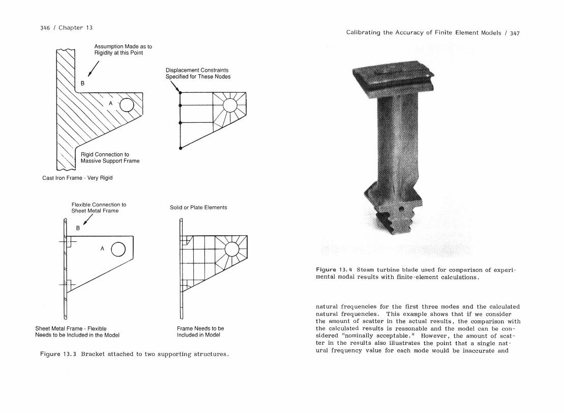
3116 / Chapter 13
Assumption Made es to Assumption Made es to Rigidity at this Point Rigidity at this Point
Rigid Connection to Rigid Connection to Massive Support Frame Massive Support Frame
Cast Iron Frame Very Rigid
Flexible Connection to Sheet Metal Frame ,
Sheet Metal Frame - Flexible Needs to be Included in the Model
Displacement Constraints Specified for These Nodes
Solid or Plate Elements
Calibrating the Accuracy of Finite Element Models I 347
Figure 13.4 Steam turbine blade used for comparison of experi- mental modal results with finite-element calculations.
natural frequencies for the first three modes and the calculated natural frequencies. This example shows that if we consider the amount of scatter in the actual results, the comparison with the calculated results is reasonable and the model ten be con- sidered “nominally acceptable. I’ However, the amount of scat- ter in the results also illustrates the point that e single nat- ural frequency value for each mode would be inaccurate end Figure 13.3 Bracket attached to two supporting structures.
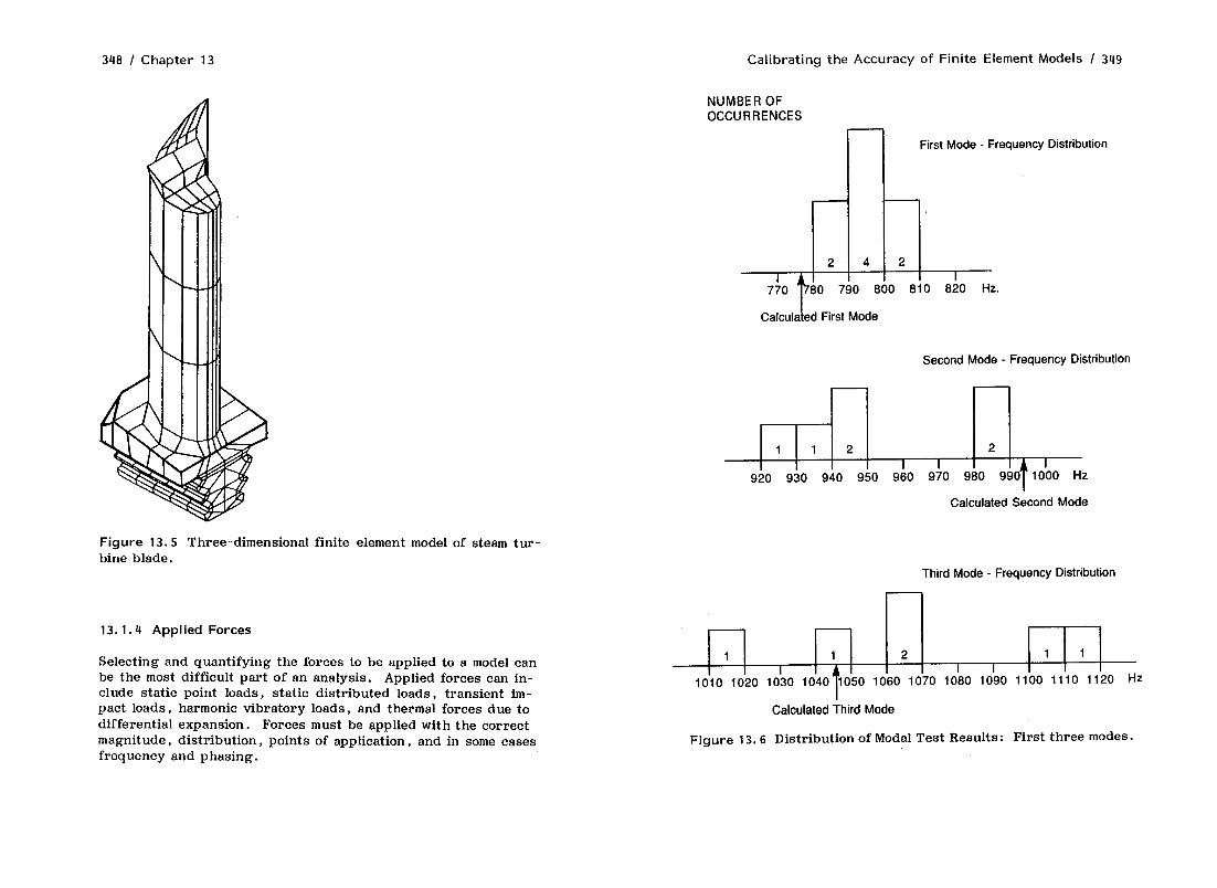
348 I Chapter 13 Calibrating the Accuracy of Finite Element Models / 349
NUMBER OF OCCURRENCES
r-l
First Mode - Frequency Distribution
2 4 2 I I
770 80 790 800 810 820 Hz.
Calculated First Mode
Second Mode - Frequency Distribution
pjg, , n+, 920 930 940 950 980 970 980 990 1000 Hz
Calculated Second Mode
Figure 13.5 Three-dimensional finite element model of steam tur- bine blade.
Third Mode - Frequency Distribution
13.1.4 Applied Forces
Selecting and quantifying the forces to be applied to a model can be the most difficult part of an analysis. Applied forces can in- clude static point loads, static distributed loads, transient im- pact loads, harmonic vibratory loads, and thermal forces due to differential expansion. Forces must be applied with the correct magnitude, distribution, points of application, and in some cases frequency and phasing.
1 1 2 1 1 I I I
1010 1020 1030 1040 050 1080 1070 1080 1090 1100 1110 1120 Hz
Calculated Third Mode
Figure 13. 6 Distribution of Modal Test Results: First three modes.

350 / Chapter 13 Calibrating the Accuracy of Finite Element Models / 351
13.2 METHODS OF CALIBRATION
The calibration of finite element results may be broken down into deterministic and probabilistic methods :
Detertninistic Comparison with test results from an actual structure.
Probabilistic Mathematically bounding the problem with sen- sitivity analysis.
13.2.1 Deterministic Approach : Comparison;’ of Test Results
The most basic way of checking the accuracy of an analysis is by comparison with test data from the actual structure. Measurement techniques include the use of dial indicators and strain gages for deflections and stresses, accelerometers for the measurement of dynamic response, thermocouples for steady-state and transient temperature distributions. For determination of vibration mode shapes, experimental modal analysis equipment may be used. Sim- ple techniques for obtaining an overall stress or temperature dis- tribution include the use of brittle coatings and temperature-in- dicating coatings, respectively.
Test results can help to establish loading conditions as well as calibration of the finite element analysis. For example, in the case of rotating machinery, the assumption may be made that the only applied forces are centrifugal forces. The finite element analysis will then give stresses that are linearly proportional to rotational speed squared, and zero at zero speed. If test results show stresses that are not perfectly linear with speed squared, then this may indicate other external forces such as drag due to seals acting on the machine. If the measured stresses do not ex- trapolate to zero at zero speed, then this is an indication of in- strumentation offset or thermal expansion effects that need to be removed from the test results before comparison with finite ele- ment results. When the influence of additional forces is found, it may be removed from the test results by regression analysis for the purpose of verifying the finite element model and then added as input to the finite-element model for an updated calcu- lation .
Test techniques have the disadvantage of displaying data at only one point in the case of strain gages, pressure transducers, thermocouples, or accelerometers. This can also present prob- lems in cases of high stress or temperature gradients. In set- ting up a test for comparison with finite element calculations,
data at several points in the structure should be collected over a wide range of operating conditions. This allows for quantifi- cation of basic trends and identifies any malfunctioning trans- ducers . In the event that poor correlation is found between test data and finite element results in the first comparison, the cal- culated stress and temperature gradients should be checked. In many cases, this discrepancy may be attributed to not obtaining test (strain gage or thermocouple) and finite element results at precisely the same location and in the same direction.
13.2.2 Probabilistic Approach : Mathematically Bounding the Problem
Both the finite element uncertainty and the uncertainty due to manufacturing varia&e may be partially clarified without the availability of actual test data by bounding the input data and performing a series of parametric studies. In order to com- pletely quantify the uncertainty of any finite element result, a true probabilistic approach would be required. This would in- clude establishing the statistical distribution of all input parame- ters such as geometry, applied forcing, rigidity of boundary con- ditions, etc. These distributions for each of the input parame- ters should be tested with the finite element model and the re- sults combined using an appropriate combination law. An ex- ample of the final result can be shown in Figure 13. ‘7 for the com- bination of calculated steady stress and allowable yield strength. A complete discussion of probablistic methods is beyond the scope of the present topic, but it is given in a number of sources such as (3) and (4).
An alternative approach is to bound each’of the input parame- ters with reasonable limits and proceed to thereby test the sen- sitivity and bounds of the results. In many cases, it may be difficult to establish the statistical or probabilistic distribution of an input parameter such as a distributed force; however, it may be possible to establish reasonable upper- and lowerbound numbers.
13.2.3 Bounding Finite Element Uncertainty
This upperllowerbound approach may be applied to the finite element uncertainty as well as the manufacturing uncertainty. In order to test and bound the effects of model geometry and mesh density, the rate of convergence of a particular model may be established by running several cases with different mesh
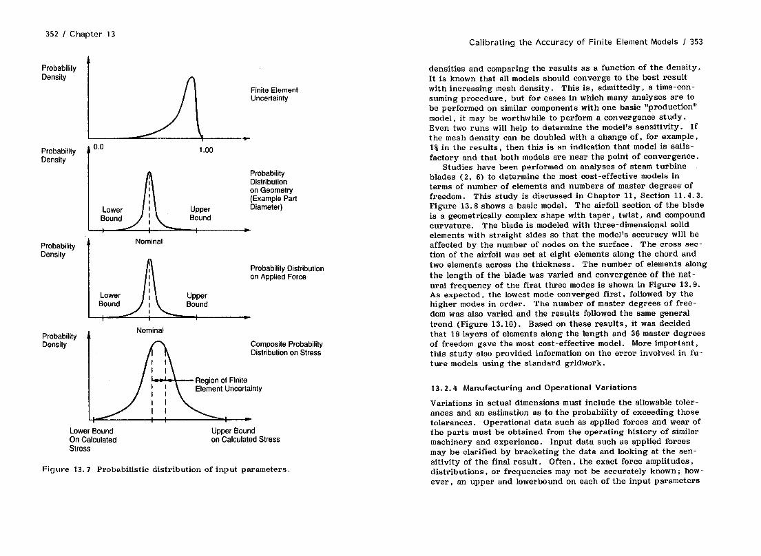
352 I Chapter 13 Calibrating the Accuracy of Finite Element Models I 353
Probability Density
Finite Element Uncertainty
c Probability
t
0.0 1 .oo Density
Probability Density
Nominal
Probability Distribution on Applied Force
Composite Probability Distribution on Stress
densities and comparing the results as a function of the density. It is known that all models should converge to the best result with increasing mesh density. This is, admittedly, a time-con- suming procedure, but for cases in which many analyses are to be performed on similar components with one basic “production” model, it may be worthwhile to perform a convergence study. Even two runs will help to determine the model’s sensitivity. If the mesh density can be doubled with a change of, for example, 1% in the results, then this is an indication that model is satis- factory and that both models are near the point of convergence.
Studies have been performed on analyses of steam turbine blades (2, 6) to determine the most cost-effective models in terms of number of elements and numbers of master degrees of freedom. This study is discussed in Chapter 11, Section 11.4.3. Figure 13.8 shows a basic model. The airfoil section of the blade is a geometrically complex shape with taper, twist, and compound curvature. The blade is modeled with three-dimensional solid elements with straight sides so that the model’s accuracy will be affected by the number of nodes on the surface. The cross sec- tion of the airfoil was set at eight elements along the chord and two elements across the thickness. The number of elements along the length of the blade was varied and convergence of the nat- ural frequency of the first three modes is shown in Figure 13.9. As expected, the lowest mode converged first, followed by the higher modes in order. The number of master degrees of free- dom was also varied and the results followed the same general trend (Figure 13.10). Based on these results, it was decided that 18 layers of elements along the length and 36 master degrees of freedom gave the most cost-effective model. More important, this study also provided information on the error involved in fu- ture models using the standard gridwork.
Lower Bound On Calculated Stress
Upper Bound on Calculated Stress
Figure 13. 7 Probabilistic distribution of input parameters.
13. 2.4 Manufacturing and Operational Variations
Variations in actual dimensions must include the allowable toler- ances and an estimation as to the probability of exceeding those tolerances. Operational data such as applied forces and wear of the parts must be obtained from the operating history of similar machinery and experience. Input data such as applied forces may be clarified by bracketing the data and looking at the sen- sitivity of the final result. Often, the exact force amplitudes, distributions, or frequencies may not be accurately known ; how - ever, an upper and lowerbound on each of the input parameters

354 I Chapter 13
Variable Number of Dynamic Degrees of Freedom
Variable Number of Element Rows Along Vane Length
8 Elements Along the Chord 2 Elements Through the Thickness
Two Nodes (4 DDOF) per Row
Dynamic Degrees of Freedom DDOF in Y and 2 Directions
X Z
-\t Y
Figure 13.8 Steam turbine blade model used for parametric stud- ies .
can usually be established. In these cases, two calculations may be run for the upper- and lowerbound cases. The results should then bound the problem, and if the worst-case results are still acceptable, the analysis may be accepted on that basis.
The combined finite element uncertainty and manufacturing variations can be shown, in principle, in Figure 13.11. The curve represents the probabilistic distribution of an actual func- tion, stress for example, which is to be predicted by finite ele- ment analysis. The finite element uncertainty is shown super- imposed on the total uncertainty curve. If each of the input
Natural Freq., Hz
750
700
650 .
Calibrating the Accuracy of Finite Element Models / 355
450
400
350 1 . .
200 -
150 -
100 I I I I I
6 12 18 24 30
Element Layers
Figure 13.9 Number of vane elements vs. natural frequencies, 18 dynamic degrees of freedom.

356 I Chapter 13 Calibrating the Accuracy of Finite Element Models / 357
Natural Natural 800 - 800 Freq., Hz
650 -
.
200 -
150 -
100 I I I I I
6 12 18 24 30
Figure 13.10 Number of dynamic degrees of freedom vs. natural frequencies, 30 layers of elements.
Probability Density Probability Due to
Combined Uncertainty
Probability Due to Finite Element Uncertainty, Alone
Lower Bound
Upper Bound
Stress
Calculated Calculated Result Result
Figure 13.11 Composite distribution of finite element results.
parameters, including finite element modeling parameters, were bounded, the results can also be shown in Figure 13.11.
In some cases, it may be difficult to see the influence of in- put parameters at the beginning of an analysis. For example, a design analysis may have the objective of determining a com- ponent’s susceptibility to fatigue that, in turn, is a combination of steady stress and dynamic stresses. The input parameters are steady force and dynamic force and its frequency. Not each of these three parameters can be quantified with the same degree of confidence, but not all of them will be as significant in deter- mining the susceptibility to fatigue. By performing a series of finite element calculations using upper and lowerbounds on each of the parameters, it may be found that the frequency of dy- namic loading, for example, is the most critical parameter be- cause of a potential resonance problem. In that case, the mag- nitude of the dynamic stresses may be critical and further effort

358 I Chapter 13
should be put into precisely defining the dynamic forcing fre- q uency range.
13.3 SUMMARY
There is no automatic answer to the question of how accurate finite element analysis is. The accuracy will vary for each in- dividual case. However, with an understanding of the basic behavior of the structure and some ingenuity reasonable, esti- mates can be given.
REFERENCES
1.
2.
3.
4.
5.
MacNeal, R. H. and R. L. Harder, “A Proposed Set of Prob- lems to Test Finite Element Accuracy,” Finite Elements in Analysis and Design, No. I, North-Holland, Amsterdam, 1985. Steele, J. M., N . F. Rieger , and T. C . T. Lam, “Develop- ment and Testing of a General Purpose Finite Element Model for Stress and Vibration Analysis of Steam Turbine Blade Groups:’ Joint Power Generation Conf., Oct. 1986, Portland, OR. Haugen, E. B., Probabilistic Approaches to Design, Wiley, New York, 1968. Wadsworth, G. P. and J. G. Bryan, Probability Theory and Random Variables,, McGraw-Hill, New York, 1960. Steele, J. M., “Finite Element Modal Analysis of Steam Tur- bine Blading,” 4th International Modal Analysis Conf., Los Angeles, Calif. , Feb. 1986.
INDEX
Accuracy, 207, 341 Computer graphics, 138 ANSYS, 2, 54 Conduction, 328 Applied forces, 47 Conductivity matrix, 330 Automatic mesh generation, Convection, 328, 332
52 Cook, R. D., 4, 189
Back-substitution, 257 Bathe, K. J., 4, 109 Body forces, 50 Boltzmann’s constant, 329
Calibration deterministic, 350 probabilistic, 356
Cheung, Y. K., 2, 4 Clough, R. W., 3
Data input format, 53 Debugging models, 131 Displacement constraints, 47,
138 Distributed forces, 50
Element accuracy, 189 aspect ratio, 191, 199, 264 bow, 192 convergence, 155
359

360 I Index
[Element] density, 207 distortion, 189, 342 gap, 270 integration order, 146, 194 isoparametric, 2 LD, 147, 198, 204 LDADS, 147, 194, 196, 198,
202, 204 missing, 135 performance, 141 plate, 194 QD, 147, 198 reduced integration order,
196 skew angularity, 192, 199 taper ratio, 191, 199, 201,
204 vertex angles, 204 warping, 192
Example case circular plate, 259 crank, 64, 75, 231 curved beam, 157 gear segment, 238, 263 notched block, 62, 74, 227 plate with circular hole, 59,
73 pressure vessel, 63, 75, 333 rectangular plate, 168 refined modeling, 226 right-angle beam, 211 rotating disk, 182 Scordelis-Lo roof, 175 simple beam, 151, 192 spherical shell, 177 thick-walled cylinder, 180 turbine blade, 68, 78, 242 turbine blade attachment,
270
Film temperature, 329
Forces, 137 Free body diagram, 72 Frontal solution, 2
Gallagher, R. H. , 4 Gear segment, 66, 76 Geometry, 133
Harder, R. H., 149, 163, 168, 175, 180, 358
Haugen, E. B., 358 Heat transfer, 327, 328 Heubner, K. H., 4
Input data, 41 Irons, B. M., 2, 3
Lo, K. S., 175
MacNeal, R. L., 149, 157, 163, 168, 175, 180, 358
MacNeal-Schwendler Corpora- tion, 1
Manufacturing variability, 342, 353
Martin, H. C., 3 Mass density, 137 Material properties, 43, 137 Mesh density, 351 Modal test, 345 Morely, L. S. D., 177 Morris, A. J., 177 MSC /NASTRAN , 54
NASTRAN, 1 Nickell, R. E., 2, 4
Finite element uncertainty, 342 Nodal forces, 49
Nodes coincident , 135 errors, 135
Nonlinear problems, 259, 270
Parametric studies, 351 Patch test, 148 Peterson, R . E. , 253 Plate-solid transitions, 247 Poisson’s ratio, 137, 181 Problem definition, 56
Radiation, 328 Refined mesh modeling, 207 Roark, R. J., 180, 188
Scordelis, A. C., 175 Seeley, F. B., 59, 80 Shrink plot, 135 Smith, J. O., 59, 80 Steam turbine, 345 Steele, J. M. , 358 Stodola, A., 183 Submodeling, 209 Substructuring, 255 Superelement, 255
Index / 361
Swanson Analysis Systems, Inc. , 2
Test techniques, 350 Thermal analysis, 327 Thermal effects, 253 Thermal modeling, 331 Timoshenko, S. P., 169, 183,
188 Topp, L. J., 3 Transient heat conduction, 330 Turner, M. J., 1, 3 Twisted beam, 163
Units, 43
View factor, 332
Wadsworth, G. P., 358 Wilson, E. L., 2, 4, 190
Young’s modulus, 137
Zienkiewicz, 0. C., 2, 3, 175