working paper series - european central bank · 2017-02-27 · working paper series . macro . s....

Working Paper Series Macro stress testing euro area banks' fees and commissions

Christoffer Kok, Harun Mirza, Cosimo Pancaro

Disclaimer: This paper should not be reported as representing the views of the European Central Bank (ECB). The views expressed are those of the authors and do not necessarily reflect those of the ECB.

No 2029 / February 2017

Abstract

This paper uses panel econometric techniques to estimate a macro-financial model for fee

and commission income over total assets for a broad sample of euro area banks. Using the

estimated parameters, it conducts a scenario analysis projecting the fee and commission

income ratio over a three years horizon conditional on the baseline and adverse macroe-

conomic scenarios used in the 2016 EU-wide stress test. The results indicate that the fee

and commission income ratio is varying in particular with changes in its own lag, the short-

term interest rate, stock market returns and real GDP growth. They also show that the

fee and commission income ratio projections are more conservative under the adverse sce-

nario than under the baseline scenario. These findings suggest that stress tests assuming

scenario-independent fee and commission income projections are likely to be flawed.

Keywords: Fee and commission income, stress testing, scenario analysis

JEL Classification: G21, G17, G01

ECB Working Paper 2029, February 2017 1

Non-Technical Summary

The recent financial and sovereign debt crises highlighted the importance for economic ac-

tivity of having sound banks able to withstand extreme and unexpected shocks to their balance

sheets and able to generate sufficient income even in times of distress. Indeed, banks resilient to

stress and able to act as effective financial intermediaries over the economic cycle are a necessary

condition for ensuring a smooth flow of credit to the real economy also in periods of economic

turbulence. With the aim of ensuring a well-functioning financial system to support economic

growth, macro stress-testing frameworks are often used to assess in a forward-looking manner

the resilience of the banking sector to (adverse) macroeconomic and financial developments.

The main purpose of macro stress testing is to assess the sensitivity to adverse macroe-

conomic and financial developments of individual banks’ balance sheet and profits and losses.

While most stress testing tools typically have well-developed modules for projecting loan losses

and net interest income, other sources of income and expenses are often only modelled in a

rudimentary fashion. This ignores that other parts of banks’ net income may be also related

to macroeconomic and financial developments. In other words, these stress testing approaches

may risk overlooking key elements of banks’ income generating activities, such as income from

fees and commissions which together with net interest income and net trading income are the

three most important income sources for most banks. In fact, fees and commissions constitute

on average between 22% and 30% of euro area banks’ net revenue and about two thirds of

euro area banks’ total non-interest income. Therefore, stress tests that ignore the sensitivity to

macroeconomic conditions of such an important income source may potentially underestimate

the volatility of banks’ solvency position when exposed to stress events.

Against this background, this paper proposes a model for estimating the relationship between

some key macroeconomic and financial factors and fee and commission income over assets, using

yearly data between 1995 and 2015 for a large sample of euro area banks. Then, it shows how the

estimated model can be applied to stress test the resilience of this source of revenue conditional

on the baseline and adverse macroeconomic scenarios used in the 2016 EU-wide stress test.

More specifically, the empirical strategy adopted in this paper begins with the selection, out

of a predetermined group of macroeconomic and financial factors, of the independent variables

that have the most explanatory power for fee and commission over assets, our variable of interest.

This selection approach yields as the most relevant drivers the lag of fee and commission income

over total assets, the lag of the first difference of the short term interest rate, the stock market

returns (both the lagged and the contemporaneous variable), the lag of the first difference of the

long term interest rate, residential property price growth and the real GDP growth. In a second

step, a model for fees and commissions over assets including the selected regressors is estimated.

The results show that lagged fee and commission income over assets, the contemporaneous

stock market returns and real GDP growth are positively and significantly related to fees and

commissions over assets, while the first difference of the short term interest rate is negatively and

significantly associated to our variable of interest. Finally, this study provides a scenario analysis


which highlights the usefulness of the estimated model in a stress-testing context. Indeed, the

estimated parameters are used to project fee and commission income over assets over a three

year horizon conditional on both a baseline and an adverse macroeconomic scenario. This

scenario analysis illustrates how fees and commissions over assets, aggregated at country level

for 18 euro area countries, are sensitive to the different macroeconomic developments. Indeed,

the resulting fees and commissions projections are considerably more conservative under the

adverse scenario than under the baseline scenario.

This paper contributes to the existing limited literature on the topic in several ways. First,

combining bank-level and macroeconomic data, it studies the determinants of fees and com-

missions as a ratio of total assets at the international level while most of the related studies

have investigated this issue at the country level. The international analysis is useful as provides

for a larger size of the panel and it allows for assessing country-specific differences in fee and

commission income dynamics. Second, it relies on a sound statistical technique to select, out

of a predetermined set of macroeconomic and financial factors, the determinants of fees and

commissions over assets to be included in the benchmark model. The application of this selec-

tion strategy is particularly relevant because it reduces the degree of discretion in the choice of

the key explanatory factors. Finally, this work, relying on different econometric approaches to

estimate the relationship between our variable of interest and the selected macroeconomic and

financial factors, provides the necessary degree of robustness.


1 Introduction

The recent financial and sovereign debt crises highlighted the importance for economic activity

of having sound banks able to withstand extreme and unexpected shocks to their balance sheets

and able to generate sufficient income even in times of distress. Indeed, banks resilient to stress

and able to act as effective financial intermediaries over the economic cycle are a necessary

condition for ensuring a smooth flow of credit to the real economy also in periods of economic

turbulence. With the aim of ensuring a well-functioning financial system to support economic

growth, macro stress-testing frameworks are often used to assess in a forward-looking manner

the resilience of the banking sector to (adverse) macroeconomic and financial developments,

see e.g. the studies by Henry and Kok (2013) outlining the European Central Bank (ECB)

top-down stress testing framework and by Borio, Drehmann and Tsatsaronis (2014) discussing

strength and weaknesses of macro stress testing in general.

The main purpose of macro stress testing is to assess the sensitivity to adverse macroeco-

nomic and financial developments of individual banks’ balance sheets and profits and losses.

The topic has received substantial attention in recent years and sophisticated methods have

been developed to provide sufficiently robust and conservative model predictions; see e.g. Gross

and Poblacion (2015) who promote the use of Bayesian model averaging. While most stress

testing tools typically have well-developed modules for projecting loan losses and net interest

income, other sources of income and expenses are typically only modelled in a rudimentary

fashion. This ignores that other parts of banks’ net income may be also related to macroe-

conomic and financial developments. In other words, these stress testing approaches may risk

overlooking key elements of banks’ income generating activities, such as income from fees and

commissions which together with net interest income and net trading income are the three most

important income sources for most banks. In fact, fees and commissions constitute on average

between 25% and 30% of euro area banks’ total income and about two thirds of euro area banks’

total non-interest income. Therefore, stress tests that ignore the sensitivity to macroeconomic

conditions of such an important income source may potentially underestimate the volatility of

banks’ solvency position when exposed to stress events.

Against this background, this paper proposes a model for estimating the relationship between

some key macroeconomic and financial factors and fee and commission income over assets, using

yearly data between 1995 and 2015 for a large sample of euro area banks. Then, it shows how

the estimated model can be applied to stress test the resilience of this source of revenue under

both a baseline and an adverse macroeconomic scenario.

While substantial research efforts have been directed at modelling banks’ balance sheets and

at forecasting loan losses and net interest income components, only few studies have focused

on fee and commission income despite its significance as the second most important source of

revenue for the majority of European banks. Perhaps owing to the scarcity of empirical studies

on the determinants of fees and commissions and to the fact that fee and commission income

tends to be less volatile than the other main streams of bank revenue (e.g. net interest income),


this income component is often assumed to be stable in forward-looking analyses such as stress

tests. However, this assumption may often end up being over-simplistic because a relative sta-

bility may not necessarily imply an absence of cyclical fluctuations. In fact, notwithstanding the

limited relative volatility, fee and commission income has proven to exhibit pronounced cyclical

tendencies in some cases. Fee and commission income of euro area significant banking groups

has generally tended to correlate strongly with net interest income over the last few years.1 This

seems to suggest that both sources of income are driven by some common underlying factors,

such as broad macroeconomic activity and retail customer business activities.2 Activities of

a cyclical nature probably relate to economic and financial market activities, such as financial

services (including those to retail customers), securities and loan underwriting, advisory services

related to mergers and acquisitions (M&A) and securities brokerage business. However, also

more structural factors, such as payment transactions, safe custody administration and bank

competition, are likely to be important determinants of overall fee and commission income. By

contrast, the movement of fee and commission income in relation to trading income has been

more heterogeneous across banks in the significant banking groups sample.3

The empirical literature aiming to measure the cyclical variation in non-interest income

subcomponents was pioneered by Saunders and Walter (1994) and Kwan and Laderman (1999).

These studies find that fee and commission activities provide stability to banks’ income contrary

to trading activities. ECB (2000) finds similar results for EU banks but it goes one step further

by making a distinction, within fee and commission income, between the so called traditional

fee-generating banking activities and more market-related businesses in which banks expanded

heavily in recent decades (e.g. brokerage, M&A, underwriting). Fee and commission income

from traditional banking appears to be less subject to cyclical variations compared to that

generated by recent activities. Smith, Staikouras and Wood (2003) also highlight that non-

interest income activities are less volatile than net interest income for a panel of EU banks

between 1994 and 1998. Overall, the results of the literature which studies the relationship

between non-interest income and banks’ financial performance, as well as risk-taking are not

conclusive.

Possibly, the closest study in spirit to ours is Coffinet, Lin and Martin (2009) who exploit

a large data set of French banking supervisory data between 1993 and 2007. Coffinet et al.

(2009) first detect the determinants of the three main components of banks’ revenues, i.e.

net interest income, fees and commissions and trading income, and then assess the sensitivity

of these sources of income to macroeconomic and financial developments, stress testing their

resilience to several scenarios. As regards the main drivers of fee and commission income, using

1See also the evidence provided in ECB (2013b).2This is not surprising as many products offered by banks have both an interest rate and a fee component

(e.g. customer accounts and various forms of credit agreements).3This may reflect the fact that, although trading activity can trigger fee and commission income, it can be

highly volatile (on account of price valuation adjustments) during periods of turbulence that do not necessarilyaffect banks’ trading-related fees and commissions (which are linked to business volumes). Although such animperfect correlation may suggest some potential diversification effects, the findings of the academic literatureare ambiguous in this regard (see, for example, Stiroh and Rumble (2006)).


a dynamic panel approach, Coffinet et al. (2009) show that GDP growth, stock market returns

and expenditures over total assets exhibit a positive and significant relationship while the ratio

of loan loss provisions over total loans (a measure of banks’ risk taking) is negatively related to

this source of income. The study also shows that lagged trading income has a positive impact

on current fee and commission income. Finally, the authors somewhat surprisingly find that

fees and commissions are more sensitive to adverse macroeconomic developments than interest

income.

In a related study, Lehmann and Manz (2006) likewise investigate which macroeconomic

variables play a role in explaining the earnings of the banking sector. Exploiting Swiss banking

data between 1994 and 2007, they study the main determinants of four components of banks’

earnings, i.e. net interest income, provisions, trading income and commission income, and assess

their sensitivity to different economic scenarios. In relation to the latter source of income, their

results show that lagged commissions and positive stock market returns are positively associated

with higher commission income while stock market volatility is negatively associated with this

source of income.

Albertazzi and Gambacorta (2009) investigate the relation between bank profitability at

country level and the business cycle by using annual data for 10 advanced economies between

1981 and 2003. Using a GMM estimator as suggested by Arellano and Bond (1991), they find

that non-interest income is positively and significantly related to its own lag, to stock market

volatility and the inflation rate, while negatively and significantly related to long-term interest

rates. Their empirical evidence also shows that GDP growth is not a significant driver of this

source of income.

Hirtle, Kovner, Vickery and Bhanot (2014) introduce a top-down stress-test model (called

CLASS, i.e. Capital and Loss Assessment under Stress Scenarios) to assess the impact of severe

macroeconomic developments on the performance and capital positions of US banks. In this

context, using publicly available data, they show that non-trading non-interest income over total

assets exhibit a positive significant relationship with its own lag, stock market returns and the

share of credit card loans over interest earning assets while it exhibits a negative and significant

relationship with the share of commercial real estate loans over interest earning assets and the

share of the banks assets over the total industrys assets.

Covas, Rump and Zakrajsek (2014) propose a fixed-effect quantile autoregressive approach

to study the effects of adverse macroeconomic scenarios on the capital positions of the 15 largest

US banks. Using publicly available quarterly data from 1997 to 2011, they find that non-trading

non-interest income over consolidated assets is positively and significantly associated with its

own lags while it is negatively and significantly related to three-month Treasury yield and to

corporate bond credit spreads.

Finally, in the context of the literature that studies the implications of banks income di-

versification on banks risk taking, DeYoung and Rice (2004) and Busch and Kick (2009) also

provide empirical evidence on the determinants of non-interest income.


DeYoung and Rice (2004), exploiting data for a large panel of urban US commercial banks

between 1989 and 2001, show that non-interest income is significantly associated with a number

of bank-specific factors, market conditions and technological developments. Specifically, they

find that well-managed banks, measured by a high relative return on equity (ROE), rely less

on non-interest income while large banks and banks that focus more on relationship banking

are more reliant on non-interest income. Moreover, they show that an increase in non-interest

income is related to higher and more volatile profits and an overall worsening of the risk-return

trade-off for the average commercial bank during the considered sample period.

Busch and Kick (2009) study the determinants of non-interest income and the impact of

this income source on the performance of German banks between 1995 and 2007 using yearly

supervisory data. Their work shows that banks relying more on traditional banking relation-

ships, holding a higher amount of equity over assets and having a higher service intensity are

more concentrated in the fees and commissions business. Furthermore, they find that a larger

share of fee income over total income is positively and significantly associated with higher risk-

adjusted return on equity (ROE) and on total assets (ROA). However, for commercial banks

they provide evidence that a strong involvement in fee-generating activities is associated with

higher risk.

This paper contributes to the existing limited literature in several ways. First, combining

bank-level and macroeconomic data, it studies the determinants of fees and commissions as a

ratio to total assets and stresses this source of income at the international level while most of

the related studies have investigated this issue at the country level. The international analysis

is useful as it provides for a larger size of the panel and allows for assessing country-specific

differences in fee and commission income dynamics. Second, it relies on a sound statistical

technique (i.e. the Least Angle Regression procedure (LARS) developed by Efron, Hastie,

Johnstone and Tibshirani (2004)) to select, out of a predetermined set of macroeconomic and

financial factors, the determinants of fees and commissions over assets to be included in the

benchmark model. The application of this selection strategy is particularly relevant because it

reduces the degree of discretion in the choice of the key explanatory factors. This is similar in

spirit to the approach by Kapinos and Mitnik (2016), who employ the Least Absolut Shrinkage

and Selection Operator (LASSO), which is a constrained version of LARS, in a stress testing

framework. Finally, our study hinges on four different econometric approaches to estimate

the drivers of fees and commissions over assets and, thus, provides the necessary degree of

robustness.

Our empirical strategy begins with the selection, out of a predetermined group of macroeco-

nomic and financial factors4, of the independent variables that have the most explanatory power

for fees and commission over assets. To this end, we exploit the LARS procedure developed by

Efron et al. (2004). Then, in a second stage, we estimate a benchmark model according to 4

different econometric methods: we employ a feasible generalised least square (FGLS) estimator,

4In this analysis, we only consider macroeconomic and financial variables as possible explanatory factors of feeand commission income over assets as these are the variables which are typically included in stress test scenarios.


a fixed effects (FE) model, a system generalized methods of moment (GMM) estimator (Blun-

dell and Bond 1998) and a bias-corrected least squares dummy variable (LSDVC) estimator as

implemented by (Bruno 2005a,b). The latter method represents our preferred approach since

it corrects for dynamic panel bias, induced by the inclusion of the lagged dependent variable

among the selected regressors, while still allowing for the explicit estimation of bank fixed effects.

Our benchmark estimates, using as explanatory variables the lag of the dependent variable,

the stock market returns (both lagged and contemporaneous value), GDP growth, both the lag

of the first difference of the short-term and long-term interest rates and the residential property

price growth, show that the signs of the estimated coefficients are all as expected when significant

and broadly in line with the previous literature. More specifically, our results show that lagged

fee and commission income over assets, stock market returns and GDP growth are positively

and significantly related to fees and commissions over assets, while the first difference of the

short-term interest rate is negatively and significantly associated with our dependent variable.

The other variables are insignificant. Against this background, it is important to stress that

the different econometric methods adopted yield qualitatively similar results. The results are

also resilient to a set of robustness checks.

Finally, as a last step of our investigation, we conduct a scenario analysis. We use the esti-

mated parameters to project fee and commission income over assets over a three-year horizon

(between 2016 and 2018) conditional on both the baseline and adverse financial and macroe-

conomic scenarios used in the 2016 EU-wide stress test exercise coordinated by the European

Banking Authority (EBA). This scenario analysis illustrates how fees and commissions are sen-

sitive to the different macroeconomic developments. Indeed, the resulting fee and commission

projections aggregated at country level are considerably more conservative under the adverse

scenario than under the baseline scenario. More specifically, the projected fee and commission

income ratios feature, at country level, an overall decline with respect to the 2015 starting

point under the adverse scenario for the majority of countries. By contrast, baseline projections

exhibit either a steady or an increasing path with respect to the 2015 cut-off level for most of

the countries.

The rest of this paper is organized as follows. In Section 2, we describe the dataset we use

in our analysis. In Section 3, we present some descriptive information for the key variables

of interest; Section 4 outlines the applied variable selection procedure. Section 5 reports the

adopted econometric approaches, displays and discusses our main findings, and briefly describes

the implemented battery of robustness checks. Section 6 illustrates the scenario analysis that

we conduct according to both a baseline and an adverse scenario. A final section concludes.

2 Data

In this study, we use an unbalanced panel of annual data from 1995 to 2015 for a sample of

banks which are mostly subject to the direct supervision of the Single Supervisory Mechanism


(SSM) and are established in all 19 euro area countries.5 The banking data were extracted

from Bloomberg. After excluding from the sample the banks for which less than 5 years of

observations are available, the dataset includes 103 banks.6 The most represented countries are

Germany (20 banks), Italy (14 banks), Spain (12 banks) and France (10 banks). One country,

namely Estonia, has only one banking institution in the sample. As expected, the coverage of

banks tends to increase over time, i.e. the most recent years typically have the best coverage.7

Table A.2 and Table A.3 provide the number of banks available in the sample respectively by

country and by year.

The bank-specific variables included in our sample are both from banks’ income statements

and balance sheets.8 In particular, from banks’ income statements we obtain information about

the variable of interest, i.e. fee and commission income. This item includes revenues earned

from a range of activities, i.e. service charges, loan servicing fees, brokerage fees, trust fees and

management fees. In this work, we only aim to model income from fees and commissions since

it is the main component of the broader non-interest income class which comprises revenues

from very heterogeneous activities. From banks’ balance sheet, we extract information about

total assets.

The dataset set used in this study also includes a series of macroeconomic and financial

variables for the considered 19 euro area countries.9 The set of explanatory variables was

selected to reflect variables considered in the literature and also taking into account the need

to include only variables that are projected in stress testing scenarios.

Finally, Table A.6 reports the main summary statistics of the used variables.

3 Some stylised facts

In the last decades, higher competition on traditional intermediation activities strengthened

banks’ incentives to develop non-interest income business activities.10 Specifically, several stud-

ies have emphasised the relevance of fees and commissions as a source of revenue for banks.

ECB (2010) and ECB (2013a) show that the mean ratio of net fee and commission income to

total assets of a sample of large euro area banks was between 0.4% and 0.6% in the second half

of the last decade. ECB (2013b) shows that the median ratio of net fee and commission income

5The 19 countries taken into account in the analysis, as shown in Table A.2, are Austria, Belgium, Cyprus,Estonia, Finland, France, Germany, Greece, Ireland, Italy, Latvia, Lithuania, Luxembourg, Malta, Netherlands,Portugal, Spain, Slovenia and Slovakia.

6The names of the banks included in the sample are reported in Table A.1. Only 31 banks out of the 103banks included in our sample have a coverage of 20 years or more.

7For the final year in the sample there are less banks available given reporting delays.8Table A.4 reports the definitions and sources of the banking variables included in the dataset.9Table A.5 reports the definitions and sources of the macroeconomic and financial variables included in the

dataset.10Stiroh (2004) shows that the share of non-interest income over net operating revenue (i.e. net interest income

plus non-interest income) increased from 25% in 1984 to 43% in 2001 for US commercial banks. ECB (2000)reports that non-interest income as a percentage of operating income has increased from 32% to 41% for Europeanbanks between 1995 and 1998.


to total income for a sample of euro area significant banking groups has hovered between 20%

and 25% in the last years. ECB (2013a) confirms this range but stresses that there is a large

heterogeneity across euro area countries. In some countries like Finland, France and Italy, the

share of fee and commission income over net income reaches levels of around 30%, whereas in

countries like Greece or Ireland this ratio is closer to 15%.

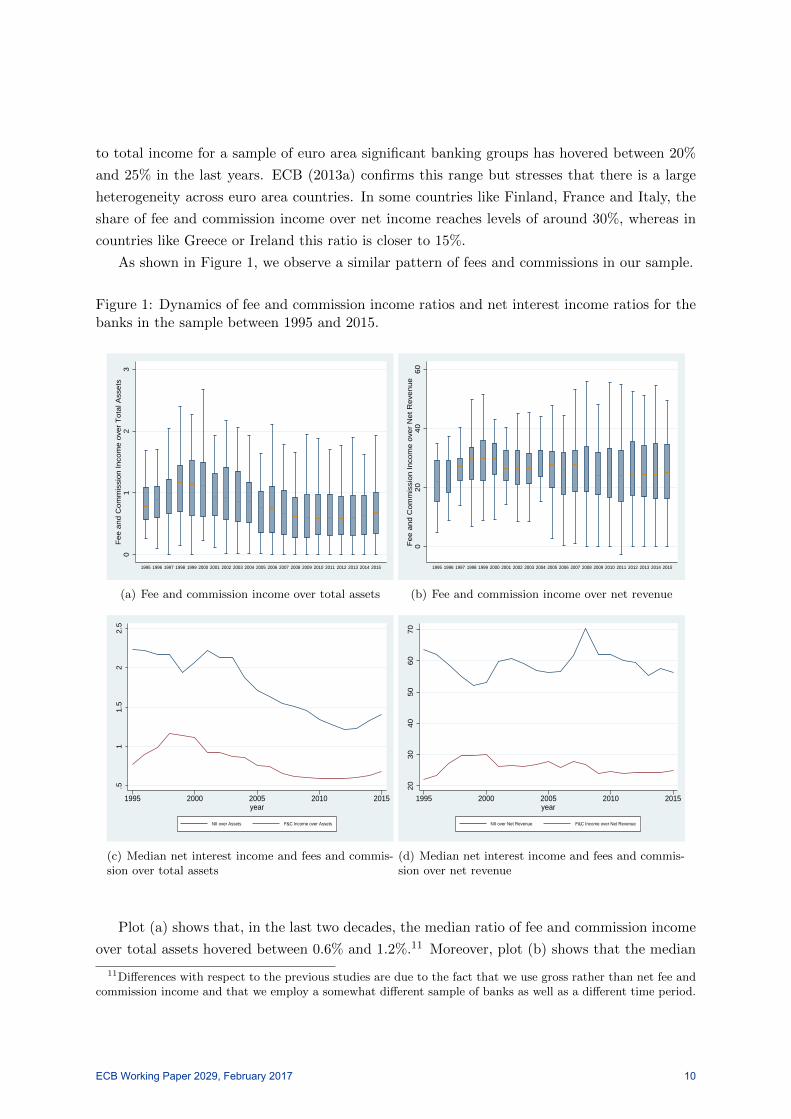
As shown in Figure 1, we observe a similar pattern of fees and commissions in our sample.

Figure 1: Dynamics of fee and commission income ratios and net interest income ratios for thebanks in the sample between 1995 and 2015.

01

23

Fee a

nd C

om

mis

sion Inco

me o

ver

Tota

l Ass

ets

1995 1996 1997 1998 1999 2000 2001 2002 2003 2004 2005 2006 2007 2008 2009 2010 2011 2012 2013 2014 2015

(a) Fee and commission income over total assets

020

40

60

Fee a

nd C

om

mis

sion Inco

me o

ver

Net R

eve

nue

1995 1996 1997 1998 1999 2000 2001 2002 2003 2004 2005 2006 2007 2008 2009 2010 2011 2012 2013 2014 2015

(b) Fee and commission income over net revenue

.51

1.5

22.5

1995 2000 2005 2010 2015year

NII over Assets F&C Income over Assets

(c) Median net interest income and fees and commis-sion over total assets

20

30

40

50

60

70

1995 2000 2005 2010 2015year

NII over Net Revenue F&C Income over Net Revenue

(d) Median net interest income and fees and commis-sion over net revenue

Plot (a) shows that, in the last two decades, the median ratio of fee and commission income

over total assets hovered between 0.6% and 1.2%.11 Moreover, plot (b) shows that the median

11Differences with respect to the previous studies are due to the fact that we use gross rather than net fee andcommission income and that we employ a somewhat different sample of banks as well as a different time period.


ratio of fees and commissions over net revenue remained rather stable between 22% and 30%.

Although this ratio is only half of that of net interest income over net revenue, it still indicates

that fees and commissions are an important source of revenues for European banks. We also

observe differences across countries. While this ratio lies between 20% and 30% for the bulk

of the 19 countries in our sample, there are few countries either somewhat below the 20%

mark (Belgium, Ireland, Malta, Netherlands) or above the 30% mark (Estonia, Italy, Latvia,

Slovenia). Furthermore, plot (c) compares the evolution of fee and commission income over

assets with that of net interest income over assets in our sample and shows that the former

ratio has overall remained rather stable over the considered time period while the latter ratio

has significantly decreased as a result of the general decline of the level of interest rates over

the past decade and in light of the financial crisis. Only recently, net interest income has picked

up again in a somewhat more benign financial environment. Moreover, it is also of interest

to compare the evolution of fees and commission income over net revenue with that of net

interest income over net revenue. As we can observe from plot (d), the median share of fees

and commissions over net revenue, while relatively stable, has increased over the early years of

our sample to peak around 2000. It then decreased slightly, but it still remains at a higher level

than it was in the beginning of the sample period. In contrast, the share of net interest income

has exhibited more variation over time.

Figure 2: Average asset size by number of observations available, in million euro

01

00

00

02

00

00

03

00

00

0in

mill

ion

5 6 7 8 9 10 11 12 13 14 15 16 17 18 19 20 21

by Minimum Number of Observations AvailableAverage Asset Size

Finally, in Figure 2, banks are grouped according to their number of available observations

and the mean asset size for each group of banks is shown. The minimum number of observa-

tions available is five, while the maximum number of observations available is 21 observations.

Notably, the average asset size is about 40% larger for the last group of banks than for the first

group of banks (e274 billion compared to e194 billion, respectively). This finding indicates


that banks with a larger coverage in terms of observations in our sample are also larger banks.

To take this fact into account we employ the ratio of fee and commission income to total assets

for our empirical analysis.

4 Variable Selection: the Least Angle Regression procedure

As also suggested by some earlier studies surveyed in Section 1, there is a large set of candidate

factors that may be associated with developments in the ratio of fee and commission income to

total assets. In order to examine which variables are the most relevant in influencing fee and

commission income over assets, we apply a variable selection procedure. More precisely, in the

presence of many candidate variables, the objective is to choose as regressors those variables

that have the most explanatory power for our variable of interest, while keeping the model

relatively sparse to avoid over-fitting problems.

For the purpose of variable selection, we employ the Least Angle Regression (LARS) al-

gorithm as developed by Efron et al. (2004) that can be seen as a generalization of the Least

Absolute Shrinkage and Selection Operator (LASSO) by Tibshirani (1996) and Foreward Stage-

wise Linear Regression (henceforth Stagewise), which is employed by Kapinos and Mitnik (2016)

in a stress testing context. The LASSO and Stagewise are constrained versions of the LARS

algorithm.12

The LASSO is a shrinkage and selection method for linear regressions which minimizes

the residual sum of squares while imposing a bound on the sum of the absolute regression

coefficients in the model thereby shrinking some coefficients towards zero. Stagewise follows

a similar approach. However, in this case, the regression function is built successively. More

precisely, the procedure starts with all the coefficients being at zero and then with small steps

ε moves in the direction of the most correlated variables with the respective residual at each

step.

The LARS approach, which derives its name from the underlying geometry, is also a stepwise

procedure that implies equiangular movements towards a predictor variable which is as highly

correlated with the residual as are the other variables already used in the prediction.13 To

perform variable selection, Efron et al. (2004) suggest making use of Mallow’s Cp statistic,

a standard information criterion, which is often used as a stopping rule in a model selection

context. The algorithm developed by the authors is computationally efficient as it only requires

as many computational steps (linear regressions) as are candidate variables available.

12As explained by Efron et al. (2004) the LARS algorithm can also be employed to compute either a LASSOor a Stagewise solution. The results are very similar for these three approaches.

13The LARS procedure also starts with the coefficients being zero and then increases the coefficient of themost highly correlated predictor x1 until the residual from the prediction is as highly correlated with a secondpredictor x2. At this point the algorithm proceeds, in contrast to the Stagewise procedure, in a directionequiangular between x1 and x2 until a third variables x3 is as highly correlated with the residual. Once more thealgorithm moves in equiangular fashion towards these three predictors until a fourth variable x4 exhibits as highcorrelation with the residual and so on.


As explained above, the LARS algorithm allows selecting a subset of regressors from a

predetermined larger set of variables and provides an order of inclusion reflecting the importance

of each independent variable in explaining the variable of interest. In this analysis, the initial

set of variables, to which the LARS algorithm is applied, comprises lagged fee and commission

income over assets and both the contemporaneous value and the first lag of those macro-financial

variables which are available for the scenario analysis, namely: stock market returns, the CPI

inflation rate, real GDP growth, the first difference of the short-term rate, the first difference

of the long-term rate and residential property price inflation. This set of variables is consistent

with economic rationale and in line with the main factors discussed in the related literature.

While arguably also variables related to banks’ financial market activity, such as brokerage and

M&A financing could be relevant, in the model presented in this paper we rely on macro-financial

factors as these are the variables which are typically included in stress test scenarios. Therefore,

our variable set is largely determined by the list of variables available in the macro-financial

scenarios used in the 2016 EU-wide stress test.

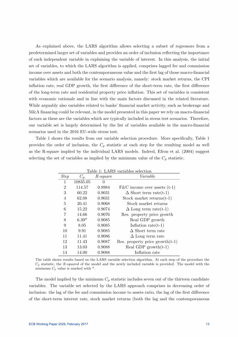
Table 1 shows the results from our variable selection procedure. More specifically, Table 1

provides the order of inclusion, the Cp statistic at each step for the resulting model as well

as the R-square implied by the individual LARS models. Indeed, Efron et al. (2004) suggest

selecting the set of variables as implied by the minimum value of the Cp statistic.

Table 1: LARS variables selectionStep Cp R-square Variable

1 10835.05 02 114.57 0.8984 F&C income over assets (t-1)3 60.22 0.9031 ∆ Short term rate(t-1)4 62.08 0.9031 Stock market returns(t-1)5 20.41 0.9068 Stock market returns6 15.22 0.9074 ∆ Long term rate(t-1)7 14.66 0.9076 Res. property price growth8 6.39* 0.9085 Real GDP growth9 8.05 0.9085 Inflation rate(t-1)10 9.91 0.9085 ∆ Short term rate11 11.41 0.9086 ∆ Long term rate12 11.43 0.9087 Res. property price growth(t-1)13 13.03 0.9088 Real GDP growth(t-1)14 14.00 0.9088 Inflation rate

The table shows results based on the LARS variable selection algorithm. At each step of the procedure theCp statistic, the R-squared of the model and the newly included variable is provided. The model with theminimum Cp value is marked with *.

The model implied by the minimum Cp statistic includes seven out of the thirteen candidate

variables. The variable set selected by the LARS approach comprises in decreasing order of

inclusion: the lag of the fee and commission income to assets ratio, the lag of the first difference

of the short-term interest rate, stock market returns (both the lag and the contemporaneous


value), the lag of the first difference of the long-term interest rate, real GDP growth and

residential property price inflation. These seven variables are included as regressors in our

benchmark model.

5 Empirical strategy and results

In the following section, we first present the econometric methods used to estimate the relation-

ship between the fee and commission income ratio to assets and the set of variables identified by

the application of the LARS and then we report and comment the regression results. Finally,

we perform a sequence of robustness checks to assess the stability and reliability of the results.

5.1 Econometric framework

Fee and commission income, like other sources of income, is driven both by the macro-financial

environment and by bank-specific characteristics. However, the aim of this analysis is to shed

more light on the relationship between the variables identified by the application of the LARS

and the fee and commission income to asset variable for the banks in our sample.14 To conduct

this study, we apply different panel econometric methods. First, we use a FGLS estimator

corrected for heteroskedasticity to estimate the following model:

yi,t = φyi,t−1 + Xtβ + εi,t (1)

where yi,t is the variable of interest (i.e. fee and commission income to total assets) for each

individual bank i at time t. Fee and commission income is scaled by total assets to account

for the different size of banks in the sample. The relative average stability and persistency15 of

the fee and commission income-to-total asset ratio over time suggests that the lag of the ratio

might be a strong predictor of its contemporaneous value. Therefore, equation 1 features as

explanatory factor yi,t−1, i.e. the lagged dependent variable. Finally, Xt is a [1xj] vector and

represents the j explanatory variables16 selected applying the LARS and εi,t is the zero-mean

bank-specific error term.

In the second econometric approach, we estimate a fixed effects (FE) model to account for

bank-specific unobserved factors that might drive individual banks results. Estimating a FE

14This investigation focuses particularly on the role played by macroeconomic and financial factors as thesevariables are generally included in macroeconomic scenarios used for stress test purposes. However, bank-specificfactors are also considered as part of our robustness analysis.

15In this context, a unit root hypothesis can be rejected. Results based on Fisher-type tests (AugmentedDickey-Fuller and Phillips-Perron) are available from the authors upon request.

16As we employ a European sample, where differences in the macroeconomic environment of individual countriesexist, we use country-specific macro variables. However, a possible caveat of this approach is the fact that banksare exposed not only to the domestic economy, but through foreign operations also to macroeconomic conditionselsewhere. It could thus be worthwhile to construct bank-specific macroeconomic indicators reflecting each bank’sexposure to other countries; although data availability prevents us from pursuing this approach.


model implies assuming the existence of time-invariant bank-specific effects that are potentially

correlated with the individual regressors unlike in a random-effects model. In this context, we

estimate the following equation:

yi,t = αi + φyi,t−1 + Xtβ + εi,t (2)

where αi are the bank-specific fixed effects. The inclusion of a lagged dependent variable in

a panel framework might yield biased and inconsistent estimates due to the correlation between

the lagged dependent variables and the error terms (Nickell 1981) and (Kiviet 1995), so called

dynamic panel bias. To address this issue, we make use of two other estimation strategies.

First, as shown in equation 3, we employ a system GMM estimator (Blundell and Bond 1998)

that combines the original equation in levels and an equation in differences

yi,t = αi + φyi,t−1 + Xtβ + εi,t

∆yi,t = φ∆yi,t−1 + ∆Xtβ + ∆εi,t(3)

This estimator is designed for estimating models with a dynamic regressor and with inde-

pendent variables that are not strictly exogenous. However, dynamic panel data models which

use GMM estimators (Arellano and Bond 1991; Arellano and Bover 1995; Blundell and Bond

1998) are unfortunately only asymptotically efficient and have poor finite sample properties

particularly when the size of the sample is small.

Finally, we use, as our preferred estimation strategy, an LSDVC estimator as developed

by Kiviet (1995) and extended upon by Bun and Kiviet (2003) and Bruno (2005a) and Bruno

(2005b) which allows for the inclusion of a lagged endogenous variable, see equation (2). The

LSDVC estimator is our preferred method as it not only corrects for dynamic panel bias, but

it is also potentially more efficient than the GMM estimator17, and it allows for the explicit

estimation of bank-specific fixed effects. However, it is relevant to highlight that the LSDVC

estimator is designed for estimating models with strictly exogenous independent variables. We

employ this approach as implemented by Bruno (2005b), i.e. initialising the bias correction

with the Blundell-Bond (system GMM) estimator.18 To ensure that the estimated asymptotic

standard errors of the LSDVC estimator yield reliable t-statistics, statistical inference for the

coefficients is based on bootstrapped standard errors (50 iterations) (Bruno 2005b).

5.2 Regression results

Our analysis has two main objectives: first, it aims at examining in more depth the relationship

between the fee and commission income ratio and the set of variables identified by the application

17As shown by Kiviet (1995), Judson and Owen (1999) and Bun and Kiviet (2003), who investigated the biasesintroduced by different dynamic panel estimators using Monte Carlo experiments.

18As discussed by Bun and Kiviet (2003) and Bruno (2005b), the choice of initial estimator has only a marginalimpact on the final results.


of the LARS; second, it strives to develop a model that can be used for scenario analysis in a

stress testing context. In this regard, the estimated parameters can be used to project the fee

and commission income ratio into the future taking as input the macroeconomic projections

from a specific scenario.

Table 2 shows the regression results based on the variable set selected by the LARS: the lag

of the fee and commission income to assets ratio, the lag of the first difference of the short-term

interest rate, stock market returns (both the lag and the contemporaneous value), the lag of

the first difference of the long-term interest rate, real GDP growth and residential property

price inflation. More specifically, Table 2 depicts the results for the four different econometric

approaches discussed in Section 5.1. The first column shows the estimated coefficients for the

FGLS model while the second column depicts the results for the FE approach. Finally, column

(3 ) shows the system GMM results and column (4 ) exhibits the results based on the LSDVC

estimator.

The models generally yield qualitatively similar results. In particular, the latter three models

imply both similar coefficients and significance levels.19 More precisely, for these three models

the selected macro-financial variables which are significant comprise the lag of the first difference

of the short-term rate, stock market returns and real GDP growth. Moreover, the explanatory

variables display the expected signs when significant. The lag of the fee and commission income

ratio exhibits a positive coefficient (with an estimated value ranging from 0.67 in the FE model to

0.81 in the LSDVC model) as expected given the high positive autocorrelation of the dependent

variable. Also, as expected, real GDP growth and stock market returns are positively associated

with the fee and commission income to total asset ratio. Their increases, respectively, indicate

a better performing real economy and growing financial markets which would both imply an

expansion of those financial services (e.g. M&A and securities brokerage) that generate fee and

commission income. This finding is in line with the previous literature and thus corroborates

with results reported by Coffinet et al. (2009) for real GDP growth and stock market returns

and by Lehmann and Manz (2006) and Hirtle et al. (2014) for stock market returns. The

estimated coefficient on the (lagged) first difference of the short-term rate has a significant

negative sign. This result can be justified by the following mechanism: lower short-term rates

are usually associated with higher bank business volumes, which should have a positive effect on

fee and commission income. At the same time, it may also reflect a rebalancing effect whereby

a bank changes its focus from activities generating net interest income towards more fee and

commission income-generating activities. Covas et al. (2014) also find a qualitatively similar

result.

The scale of the estimated coefficients can be interpreted in the following way: one additional

percentage point of real GDP growth would lead, ceteris paribus, to an increase in the average

fee and commission income ratio to total assets of about 1% given an average fee and commission

income ratio in our sample of 0.79%.

19In this context, it is worth underlining that the FGLS model neither includes individual fixed effects noraddresses the possible dynamic panel bias.


Table 2: Regressions for fee and commission income over assets on the selected macroeconomicand financial variables

(1 ) (2 ) (3 ) (4 )FGLS FE GMM LSDVC

F&C Income/Total Assets(t-1) 0.9801*** 0.6666*** 0.8066*** 0.8122***(175.59) (7.23) (9.29) (34.22)

∆ Short term rate(t-1) -0.0103*** -0.0174*** -0.0180*** -0.0199***(-4.81) (-4.17) (-4.79) (-4.49)

Stock market returns(t-1) 0.0003*** 0.0003 0.0003 0.0003(2.72) (1.22) (1.34) (1.14)

Stock market returns 0.0003*** 0.0005** 0.0005** 0.0006***(2.98) (2.43) (1.98) (2.60)

∆ Long term rate(t-1) -0.0039* 0.0018 -0.0009 0.0006(-1.91) (0.43) (-0.22) (0.19)

Real GDP growth 0.0012 0.0085** 0.0053* 0.0087***(1.08) (2.38) (1.77) (3.30)

Res property price growth -0.0016*** 0.0021 -0.0008 0.0005(-3.68) (1.40) (-0.64) (0.38)

Constant 0.0044 0.2255*** 0.1277**(1.27) (3.37) (2.01)

Observations 1119 1119 1119 1119Banks 103 103 103 103

Wald χ2 31671*** 299*** 1463***F -statistic 75***

AR(2) Arellano-Bond test (p-value) 0.27Hansen J test (p-value) 0.11Number of instruments 10

***, **, and * denote significance at the 1%, 5% and 10% level, respectively. Parameter estimates based onthe feasible GLS approach (FGLS), equation 1, the fixed effects approach (FE) and the LSDVC approach(LSDVC), both equation 2, and system GMM (GMM), equation 3, are shown. z-statistics (t-statistic in theFE case) based on heteroscedasticity and autocorrelation robust standard errors are shown in parenthesis.Below the parameter estimates the number of observations and the number of individual banking groups inthe sample are provided. Further, the Wald χ2 statistic (F -statistic in the case of FE model) to test for thejoint significance of the estimated parameters is given. Finally, for the GMM approach the p-value based onthe Arellano-Bond statistic to test for second-order autocorrelation and on the Hansen J statistic to test thevalidity of the overidentifying restrictions, respectively, is shown. Further, in this case the lagged dependentvariable is instrumented with its own lags (collapsed), the exogenous variables in the model and the timedummies.

The test results included for the GMM approach indicate the validity of the instruments

used, as the over-identifying restrictions are fulfilled, and further show the absence of second-

order autocorrelation in the residuals when using this estimator.20

20Results for the FGLS model stand out in yielding a much higher autocorrelation coefficient of 0.98. Thiscan be explained by the absence of any fixed effects in the model. In this model also the other macro-financialvariables have significant coefficients (in particular lagged stock market returns and residential property pricegrowth), while the coefficient on real GDP growth is not significant. Given the before mentioned caveats of thismodel, we deem these results less reliable.


5.3 Robustness checks

We perform a sequence of robustness checks to ensure the stability and reliability of the results

of our preferred model which relies on the LSDVC estimator; the results of which are shown in

Table 3.

Table 3: Robustness regressions for the LSDVC model

(1 ) (2 ) (3 ) (4 )

F&C Income/Total Assets(t-1) 0.8025*** 0.8104*** 0.8064*** 0.9102***(40.24) (33.27) (32.65) (43.70)

∆ Short term rate(t-1) -0.0136*** -0.0196*** -0.0206*** -0.0174***(-3.56) (-4.50) (-4.38) (-3.44)

Stock market returns(t-1) 0.0002 0.0003 0.0004(1.06) (1.11) (1.57)

Stock market returns 0.0006*** 0.0006*** 0.0006*** 0.0005*(2.80) (2.64) (2.59) (1.82)

∆ Long term rate(t-1) -0.0003 0.0000 0.0012(-0.10) (0.00) (0.35)

Real GDP growth 0.0103*** 0.0086*** 0.0091*** 0.0064**(6.27) (3.26) (3.37) (2.32)

Res property price growth 0.0004 0.0003 -0.0005(0.34) (0.27) (-0.40)

Inflation rate 0.0027(0.84)

Inflation rate(t-1) 0.0030(0.78)

Observations 1207 1119 1119 729Banks 103 103 103 53Wald 1760*** 1516*** 1373*** 2476***

***, **, and * denote significance at the 1%, 5% and 10% level, respectively. Parameter estimates for equa-tion 2 based on the LSDVC approach are shown. z-statistics based on heteroskedasticity and autocorrelationrobust standard errors are shown in parenthesis. Below the parameter estimates, the number of observationsand the number of individual banking groups in the sample are provided. Further, the Wald χ2 statistic totest for the joint significance of the estimated parameters is given.

We begin with removing those variables that are insignificant in the LSDVC model. In

particular, these are lagged stock market returns, the lag of the first difference of the long-term

interest rate and residential property price inflation. The results shown in column (1 ) confirm

the robustness of the results which are hardly changed in terms of the significance and the

value of coefficients of those variables left in the model. A further robustness check consists of

including additional control variables in the LSDVC benchmark model. More specifically, we

enhance the model with either the lag or the contemporaneous value of CPI inflation, as the

variable is the only that has not been picked in either form by the LARS algorithm. As shown

in columns (2 ) and (3 ) in Table 3, the main results of the analysis are robust to the inclusion of

these additional controls. Indeed, the variables, which were included in the benchmark model in


line with the results of the LARS, maintain their significance and sign. Also both the coefficient

on lag and on the contemporaneous value of inflation are insignificant in their respective models.

Therefore, there does not seem to be an omitted variable bias problem in the LSDVC model as

far as these variables are concerned.21

Finally, we test the robustness of our benchmark results by limiting the sample to only those

banks with a value of total assets larger than or equal to 50 billion which roughly halves the

sample. As shown, in column (4 ) in Table 3, the main results of the analysis do not change on a

qualitative basis. The main difference consists of a somewhat higher autocorrelation coefficient

and slightly smaller coefficients on the macro-financial variables with the coefficient on stock

market returns being on a lower significance level.

6 Scenario analysis

In this section, a scenario analysis of fee and commission income over total assets under both

a baseline and an adverse scenario for a three-year horizon between end-2015 and end-2018 for

18 euro area countries is conducted.22

The projections of fee and commission income over total assets are computed feeding the

macroeconomic scenarios through the estimated benchmark LSDVC model (presented in column

(4 ) in Table 2) which is seeded with the end-2015 bank-level data. It is worth highlighting that

bank specific fee and commission income projections are aggregated and displayed at country

level. First, the model projections are computed at bank level year by year and, then, country

level projections are generated as weighted averages of the bank level projections.

The scenarios adopted in this exercise are those employed in the 2016 EU-wide stress test

exercise coordinated by the EBA and were published in February 2016. The baseline scenario is

based on an extension of the European Commission (EC) Autumn 2015 forecast, while the ad-

verse scenario reflects a joint scenario of a reversal in global risk premia, weak financial market

profitability in a low growth environment, rising public and private debt sustainability concerns

and shocks to the shadow banking sector. For the euro area as a whole these shocks result in real

GDP growth rates falling below the baseline rate by 2.8, 3.2 and 1.1 percentage points, respec-

tively in 2016, 2017 and 2018. More information on the scenarios and the developments of the

key macroeconomic and financial variables under the baseline and the adverse macroeconomic

scenarios are reported in EC (2016) and ESRB (2016) .

In this context, it is key to emphasize that the exercise presented in this section is not a

21We also assessed the impact of including in the estimated model bank-specific variables reflecting on the bankbusiness model, namely the retail ratio and the leverage ratio. In both cases, the coefficients of the benchmarkvariables did not change substantially such that there does not seem to be an omitted variable bias problemrelated to these indicators. It is worth noting that the estimated coefficient for the retail ratio is positive andsignificant. This seems to suggest that more traditional banks on average have a higher fee and commissionincome to total assets ratio. The coefficient on the leverage ratio is negative and significant indicating that moreleveraged banks on average have lower fee and comission income. Results are available upon request.

22No projections for Lithuania are included, as there are no data points for fee and commission income for therespective banks at the end of the sample, i.e. for 2014 and 2015.


Figure 3: Projection of fee and commission income over assets aggregated at country level, %change with respect to the cut-off level

-10

-8-6

-4-2

0

2016 2017 2018

AT

-25

-20

-15

-10

-50

2016 2017 2018

BE

-50

510

15

2016 2017 2018

CY-2

0-1

5-1

0-5

0

2016 2017 2018

DE

-20

-15

-10

-50

2016 2017 2018

EE

05

10

2016 2017 2018

ES

Base, % change Adverse, % change

sensitivity analysis but a proper stress testing analysis. More specifically, this analysis studies

how consistent changes in all the relevant explanatory macroeconomic and financial factors

included in the benchmark model affect fee and commission income over the stress test horizon.

However, it is also important to note some limitations of the approach. First, potential

feedback effects between the banking sector and the real economy are not taken into account.

Second, total assets (used to compute the fee and commission income ratio) are not explicitly


Figure 3: Projection of fee and commission income over assets aggregated at country level, %change with respect to the cut-off level, cont.

-30

-25

-20

-15

-10

-5

2016 2017 2018

FI

-8-6

-4-2

02

2016 2017 2018

FR

-10

010

20

30

2016 2017 2018

GR-3

0-2

0-1

00

2016 2017 2018

IE

-4-2

02

4

2016 2017 2018

IT

-30

-20

-10

0

2016 2017 2018

LU


modelled as they are assumed to be constant over the stress test horizon.23 Third, even though

our model results seem robust to the different specifications discussed before, some open ques-

tions on model coefficient stability remain. In particular, the economic literature has emphasized

the importance of financial cycles for the conduct of macro-prudential policy, because the fi-

nancial system might evolve differently as a response to such policy during booms and busts

23However, the assumption of constant total assets is in line with the static balance sheet approach used in the2011 EBA stress test, the 2014 ECB Comprehensive Assessment stress test and the 2016 EU-wide stress test.


Figure 3: Projection of fee and commission income over assets aggregated at country level, %change with respect to the cut-off level, cont.

-10

-50

2016 2017 2018

LV

-30

-20

-10

0

2016 2017 2018

MT

-20

-15

-10

-50

5

2016 2017 2018

NL-1

0-5

0

2016 2017 2018

PT

02

46

8

2016 2017 2018

SI

-50

510

2016 2017 2018

SK


(Hiebert, Schuler and Peltonen 2015; Runstler and Vlekke 2016; Stremmel 2015). Similarly,

income elasticities might be different across financial cycles which would suggest that fee and

commission income could react differently to some financial and/or macroeconomic variables

under a baseline versus an adverse scenario. To the extent that this source of income would

react relatively stronger (weaker) to the relevant variables in a crisis scenario, the severity of

the corresponding projections would be amplified (reduced) relative to what is shown in this


section. This would further imply that elasticities might differ across countries, e.g. between

crisis and non-crisis countries. However, given the data limitations, we leave this important

topic for future research.

Figure 3 displays the projections of fee and commission income ratios aggregated at country

level for 18 euro area countries in terms of percentage changes with respect to the cut-off levels.

The light blue bars are the projected percentage changes under the baseline scenario while

the dark blue bars are the projected percentage changes under the adverse scenario. In the

Appendix, figure A.4 shows the aggregated country level projections of fee and commission

income ratios in levels. The light gray line in each graph shows the actual historical value, the

light blue line represents the baseline scenario projection and the dark blue line represents the

adverse scenario projection.

The figures show that fee and commission income projections are sensitive to the different

macroeconomic developments. As expected, the projections of fee and commission income under

the adverse scenario are consistently below the projected income under the baseline scenario.

On average, the cumulative deviation between the adverse and baseline country level projections

over the stress test horizon corresponds to 55 basis points (bps) of the 2015 CET1 ratio.24 For

the majority of countries, the projected fee and commission income ratios feature an overall

decline under the adverse scenario with respect to the 2015 starting level. An exception to

that are Cyprus, Spain and Slovenia which end up with a somewhat higher fee and commission

income ratio at the end of the scenario horizon. This can be explained by the combination of a

milder scenario for these countries and positive fixed effects for the relevant banks.

For the majority of the remaining countries, namely Finland, Austria, Belgium, Finland,

France, Greece, Italy, Luxembourg, Portugal and Slovakia, the adverse scenario projections

follows rather a V-shaped path, i.e. they first decline but then they bounce back towards their

starting level, but typically not fully. This reflects the specific characteristics of the scenario

which features first a decline in economic indicators followed by a subsequent recovery. For

the other countries examined in this exercise, the projections exhibit a continuous reduction

in fee and commission income. Overall, the countries most severely affected under the adverse

scenario in terms of the decline in fee and commission income ratio would be Belgium, Finland,

Ireland, Luxembourg and Malta. These countries would see their projection ratios decrease by

more than 20%.

By contrast, baseline projections, in most cases, exhibit either a rather steady or an increas-

ing path with respect to the 2015 cut-off level. Only the projections for Belgium, Germany,

Estonia, Finland, Ireland and Malta feature declines of more than 5% under the baseline sce-

nario.

Figure A.5 also reports the decomposition of the contribution of the explanatory factors to

24In particular, the cumulative deviation between the adverse and baseline country level projections over thestress test horizon is 43 bps for Austria, 71 bps for Belgium, 24 bps for Cyprus, 64 bps for Germany, 67 bps forEstonia, 38 bps for Spain, 90 bps for Finland, 51 bps for France, 48 bps for Greece, 50 bps for Ireland, 35 bpsfor Italy, 69 bps for Luxembourg, 83 bps for Latvia, 51 bps for Malta, 67 bps for the Netherlands, 40 bps forPortugal, 33 bps for Slovenia and 58 bps for Slovakia.


the average adverse-baseline deviation of banks’ fee and commission income over the stress test

horizon. The figure shows that in the first year of the stress test horizon real GDP growth and

the stock market returns are the largest contributors to the deviation. In the second year and

particularly in the third year, the role of these two factors declines due to the increasing effect

of the lag term of the dependent variable.

Overall, these findings point to the potential for seriously misrepresenting the sensitivity of

fee and commission income to macro-financial shocks when conducting bank stress tests where

this material income item is treated as independent from the macro scenario. Hence, explicitly

modelling fee and commission income as advertised in this study appears to be a promising

approach for future bank stress tests.

7 Conclusions

In this paper, we present an empirical macro-financial model for the estimation of fee and

commission income (as a ratio of total assets) for a broad sample of euro area banks.

In particular, in this analysis, we first employ a variable-selection technique (LARS) to

determine the set of relevant regressors for our variable of interest.

Then, using different panel econometric techniques, we find that fee and commission income

over assets is varying with the economic and financial cycle. Specifically, it is significantly

related to real GDP growth, the lag of the short-term interest rate, stock market returns and

its own lag. These results are qualitatively consistent across all the econometric approaches

applied.

Finally, as a last step of our study, we conduct a scenario analysis. We use the estimated pa-

rameters to project fee and commission income over assets over a three-year horizon conditional

on both a baseline and an adverse financial and macroeconomic scenario. This scenario analysis

illustrates how fees and commissions are sensitive to the different macroeconomic developments.

The resulting fee and commission projections aggregated at country level are considerably more

conservative under the adverse scenario than under the baseline scenario. Moreover, for the

majority of the countries, the projected fee and commission income ratios feature an overall

decline with respect to the cut-off level under the adverse scenario.

These findings suggest that stress tests assuming scenario-independent fee and commission

income projections are likely to be flawed. According to the results presented in this paper,

it is plausible that fee and commission income will differ depending on the macro-financial

environment and, ignoring this, presumably would lead to a misrepresentation of banking-sector

soundness and resilience to shocks.


References

Albertazzi, U. and L. Gambacorta, “Bank Profitability and the Business Cycle,” Journal of Financial Sta-

bility 5 (2009), 393–409.

Arellano, M. and S. R. Bond, “Some Tests of Specification for Panel Data: Monte Carlo Evidence and an

Application to Employment Equations,” Review of Economic Studies 58 (1991), 277–97.

Arellano, M. and O. Bover, “Another Look at the Instrumental Variable Estimation of Error-Components

Models,” Journal of Econometrics 68 (1995), 29–51.

Blundell, R. and S. R. Bond, “Initial Conditions and Moment Restrictions in Dynamic Panel Data Models,”

Journal of Econometrics 87 (1998), 115–143.

Borio, C., M. Drehmann and K. Tsatsaronis, “Stress-testing macro stress testing: does it live up to expec-

tations?,” Journal of Financial Stability 12 (2014), 3–15.

Bruno, G., “Approximating the Bias of the LSDVC Estimator for Dynamic Unbalanced Panel Data Models,”

Economic Letters 87 (2005a), 361–366.

———, “Estimation and Inference in Dynamic Unbalanced Panel-Data Models with a Small Number of Individ-

uals,” The Stata Journal 5 (2005b), 473–500.

Bun, M. and J. Kiviet, “On the Dimishing Returns of Higher Order Terms in Asymptotic Expansions of Bias,”

Economic Letters 79 (2003), 145–152.

Busch, R. and T. Kick, “Income Diversification in the German Banking Industry,” Deutsche Bundesbank

Discussion Paper 09, 2009.

Coffinet, J., S. Lin and C. Martin, “Stress Testing French Banks’ Income Subcomponents,” Banque de

France Working Paper 242, 2009.

Covas, F., B. Rump and E. Zakrajsek, “Stress-Testing U.S. Bank Holding Companies: A Dynamic Panel

Quantile Regression Approach,” International Journal of Forecasting 30 (2014), 691–713.

DeYoung, R. and T. Rice, “How do Banks Make Money? The Fallacies of Fee Income,” Economic Perspectives

4 (2004), 34–51.

EC, “2016 EU-wide stress test, Explanatory note on the baseline scenario,” Technical Report, European Com-

mission, 2016.

ECB, “EU Banks’ Income Structure,” (European Central Bank, 2000).

———, “EU Banking Sector Stability,” (European Central Bank, 2010).

———, “Banking Structure Report,” (European Central Bank, 2013a).

———, “The Dynamics of Fee and Commission Income in Euro Area Banks,” in Financial Stability Review

(European Central Bank, 2013b), 65–67.

Efron, B., T. Hastie, I. Johnstone and R. Tibshirani, “Least Angle Regression,” The Annals of Statistics

32 (2004), 407–499.

ESRB, “Adverse macro-financial scenario for the EBA 2016 EU-wide bank stress testing exercise,” Technical

Report, European Systemic Risk Board, 2016.


Gross, M. and J. Poblacion, “A false sense of security in applying handpicked equations for stress test

purposes,” ECB Working Paper Series 1845, 2015.

Henry, J. and C. Kok, “A macro stress testing framework for assessing systemic risks in the banking sector,”

ECB Occasional Paper Series 152, 2013.

Hiebert, P., Y. Schuler and T. Peltonen, “Characterising the financial cycle: a multivariate and time-

varying approach,” ECB Working Paper Series 1846, 2015.

Hirtle, B., A. Kovner, J. Vickery and M. Bhanot, “The Capital and Loss Assessment under Stress Scenarios

(CLASS) Model,” Federal Reserve Bank of New York, Staff Reports 663, 2014.

Judson, R. and A. Owen, “Estimating Dynamic Panel Data Models: a Guide for Macroeconomists,” Economics

Letters 65 (1999), 9–15.

Kapinos, P. and O. Mitnik, “A Top-Down Approach to Stress-Testing Banks,” Journal of Financial Services

Research 49 (2016), 1–36.

Kiviet, J., “On Bias, Inconsistency, and Efficiency of Various Estimators in Dynamic Panel Data Model,”

Journal of Econometrics 68 (1995), 53–78.

Kwan, S. and E. Laderman, “On the Portfolio Effects of Financial Convergence - A review of the Literature,”

Economic Review Federal Reserve Bank of San Francisco, 1999.

Lehmann, H. and M. Manz, “The Exposure of Swiss Banks to Macroeconomic Shocks - an Empirical Investi-

gation,” Swiss National Bank Working Papers 4, 2006.

Nickell, S., “Biases in Dynamic Models with Fixed Effects,” Econometrica 49 (1981), 1417–1426.

Runstler, G. and M. Vlekke, “Business, housing and credit cycles,” ECB Working Paper Series 1915, 2016.

Saunders, A. and I. Walter, Universal Banking in the United States. What Could We Gain? What Could We

Lose? (Oxford University Press, 1994).

Smith, R., C. Staikouras and G. Wood, “Non-Interest Income and Total Income Stability,” Bank of England

Working Paper 198, 2003.

Stiroh, K., “Diversification in Banking: Is Non-Interest Income the Answer?,” Journal of Money, Credit and

Banking 36 (2004), 853–882.

Stiroh, K. and A. Rumble, “The Dark Side of Diversification: The Case of US Financial Holding Companies,”

Journal of Banking and Finance 30 (2006), 2131–2161.

Stremmel, H., “Capturing the financial cycle in Europe,” ECB Working Paper Series 1811, 2015.

Tibshirani, R., “Regression Shrinkage and Selection via the Lasso,” Journal of the Royal Statistical Society B

58 (1996), 267–288.


Appendix

Table A.1: Sample of banksNo. Name Country Number of First Last

observations observation observation

1 BAWAG P.S.K. AT 13 2003 20152 Erste Group Bank AT 21 1995 2015

3 RZB Osterreich AT 16 2000 2015

4 RLB NO-Wien AT 8 2008 2015

5 RLB-OO AT 11 1997 20156 Argenta Group BE 8 2008 20157 AXA Bank Europe BE 6 2008 20138 Belfius Banque, S.A. BE 10 2006 20159 Dexia NV BE 21 1995 2015

10 KBC Group NV BE 21 1995 201511 Bank of Cyprus CY 21 1995 201512 Hellenic Bank Public Company Ltd CY 21 1995 201513 Aareal Bank AG DE 15 2001 201514 Bayerische Landesbank DE 17 1999 201515 Commerzbank AG DE 21 1995 201516 DekaBank Deutsche Girozentrale DE 17 1999 2015

17 Deutsche Apotheker - und Arztebank EG DE 11 2005 201518 Deutsche Bank AG DE 21 1995 201519 DZ Bank AG Dt. Zentral-Genossenschaftsbank DE 11 2005 201520 Hamburger Sparkasse AG DE 9 2007 201521 HSH Nordbank AG DE 14 2002 201522 Landesbank Baden-Wurttemberg DE 14 2002 201523 Landesbank Berlin AG DE 20 1995 201424 Landesbank Hessen-Thuringen GZ DE 15 2001 201525 Landeskreditbank Baden-Wurttemberg - Forderbank DE 9 2006 201426 Landwirtschaftliche Rentenbank DE 11 1999 201527 Mnchener Hypothekenbank eG DE 9 2007 201528 Norddeutsche Landesbank -GZ- DE 14 2002 201529 NRW.BANK DE 21 1995 201530 SEB AG DE 6 2008 201431 VW Financial Services AG DE 13 2003 201532 WGZ Bank AG Westdt. Geno. Zentralbank, Ddf DE 16 1999 201533 SEB Pank EE 11 1995 201434 ABANCA Corporacion Bancaria, S.A. ES 6 2010 201535 Banco Bilbao Vizcaya Argentaria, S.A. ES 21 1995 201536 Banco de Sabadell, S.A. ES 19 1997 201537 Banco Mare Nostrum, S.A. ES 5 2011 201538 Banco Popular Espanol, S.A. ES 21 1995 201539 Banco Santander, S.A. ES 21 1995 201540 Bankinter, S.A. ES 21 1995 201541 Banco Financiero y de Ahorros, S.A.U. ES 6 2010 201542 Ibercaja - Caja de Ahorros y Monte de Piedad de Zaragoza ES 5 2008 201243 Criteria Caixa, S.A. ES 15 1999 201344 Fundacion Bancaria Unicaja ES 16 1999 201445 Liberbank, S.A. ES 5 2011 201546 Danske Bank Oyj FI 8 2008 201547 Nordea Bank Finland Plc FI 7 2009 201548 OP Cooperative FI 17 1995 2015


Table A.1: Sample of banks, cont.No. Name Country Number of First Last

observations observation observation

49 BNP Paribas FR 21 1995 201550 BPCE SA FR 7 2009 201551 BPI Groupe S.A. FR 10 2006 201552 Groupe Credit Agricole FR 14 2002 201553 Confederation Nationale du Credit Mutuel FR 16 1999 201454 HSBC France SA FR 11 1995 201455 La Banque Postale FR 10 2006 201556 RCI Banque SA FR 12 2003 201557 Societe de financement local FR 6 2008 201458 Societe Generale FR 21 1995 201559 Alpha Bank, S.A. GR 21 1995 201560 Eurobank Ergasias, S.A. GR 18 1998 201561 National Bank of Greece, S.A. GR 21 1995 201562 Piraeus Bank, S.A. GR 21 1995 201563 Allied Irish Bank IE 21 1995 201564 The Governor and Company of the Bank of Ireland IE 6 2010 201565 Permanent TSB Group Holdings plc IE 6 2009 201466 Ulster Bank Ireland IE 9 2007 201567 Gruppo Carige IT 21 1995 201568 Gruppo Monte dei Paschi di Siena IT 20 1996 201569 Gruppo Banca Popolare dell’Emilia Romagna IT 21 1995 201570 Gruppo BPM - Banca Popolare di Milano IT 21 1995 201571 Banca Popolare di Sondrio IT 21 1995 201572 Gruppo Bancario Banca Popolare di Vicenza IT 10 2006 201573 Gruppo Banco Popolare IT 10 2006 201574 CREDITO EMILIANO SPA IT 19 1997 201575 Gruppo Bancario ICCREA IT 9 2007 201576 Gruppo Bancario Intesa Sanpaolo IT 21 1995 201577 Gruppo Bancario Mediobanca IT 21 1995 201578 Gruppo UBI Banca IT 14 2002 201579 Gruppo UniCredit IT 21 1995 201580 Gruppo Bancario Veneto Banca IT 9 2007 201581 DNB Bankas LT 7 2002 200882 NORD/ LB Lietuva LT 7 2002 200883 Banque et Caisse d’Epargne LU 13 2000 201584 Banque internationale a Luxembourg LU 9 1995 201585 ABLV Bank AS LV 7 2009 201586 Latvijas Unibanka LV 13 1995 201587 Swedbank AS (Latvia) LV 7 2009 201588 Bank of Valletta p.l.c. MT 14 1999 201589 HSBC Bank Malta p.l.c. MT 14 2002 201590 ABN Amro Group N.V. NL 11 2005 201591 BNG Bank NL 14 2002 201592 Coperatieve Centrale Raiffeisen-Boerenleenbank B.A. NL 21 1995 201593 ING Group N.V. NL 9 2007 201594 Royal Bank of Scotland N.V. NL 6 2009 201495 SNS Bank NV NL 16 2000 201596 Banco BPI, S.A. PT 21 1995 201597 Banco Comercial Portugus, S.A. PT 21 1995 201598 Caixa Geral de Depsitos, S.A. PT 12 2004 201599 Nova Kreditna Banka Maribor SI 16 1999 2015

100 Nova Ljubljanska banka d.d. SI 9 2001 2015101 Slovenska sporitelna A.S. SK 11 1995 2015102 Tatra banka SK 18 1998 2015103 Vseobecna uverova banka, A. S. SK 21 1995 2015


Table A.2: Number of banks in the sample by country

Country Number of banks

Austria 5Belgium 5Cyprus 2Estonia 1Finland 3France 10Germany 20Greece 4Ireland 4Italy 14Luxembourg 2Latvia 3Lithuania 2Malta 2Netherlands 6Portugal 3Slovenia 2Slovakia 3Spain 12

Total 103


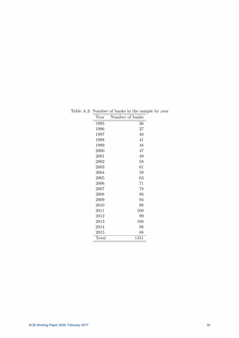
Table A.3: Number of banks in the sample by year

Year Number of banks

1995 361996 371997 401998 411999 482000 472001 492002 582003 612004 592005 632006 712007 782008 862009 942010 982011 1002012 992013 1002014 982015 88

Total 1451


Table A.4: Definition and sources of the banking variables in the datasetVariables Definitions Source

Fee and commission Commissions & fees earned; It includes commissions and fees. Bloombergincome earned from service charges, loan servicing fees, brokerage fees,

and trust fees and management fees.

Assets Sum of cash & bank balances, fed funds sold & resale agreements, Bloomberginvestments for trade and sale, net loans, investments held to maturity,net fixed assets, other assets, customers’ acceptances and liabilities

Table A.5: Definition and sources of the macroeconomic and financial variables in the datasetVariables Definitions Source

GDP growth Annual growth rate of gross domestic product ECB SDWat market price, chain linked volumes

Inflation rate Harmonised Index of Consumer Prices ECB SDW

House prices Residential property prices ECB SDW

Short-term interest rate Money market rate ECB SDW

Long-term interest rate 10y government bond yield ECB SDWStock market index National stock market index ECB SDW

Table A.6: Summary statisticsVariables Obs. Mean (in %) Std. Dev. Min Max

FC Income/Total Assets 1451 0.79 0.53 0.00 4.35Stock market returns 2014 8.85 33.52 -73.57 641.78Real GDP growth 2034 1.90 3.16 -14.81 26.28Inflation rate 2031 2.01 2.27 -13.95 14.51∆ Short term rate 1918 -0.33 1.39 -9.24 10.81∆ Long term rate 1902 -0.36 1.25 -13.98 9.58Res property price growth 1752 3.54 7.78 -38.01 52.22


Figure A.4: Projection of fee and commission income over assets aggregated at country level

.95

11.0

5

2010 2012 2014 2016 2018

AT

.25

.3.3

5.4

.45

2010 2012 2014 2016 2018

BE

.6.6

5.7

.75

.8.8

5

2010 2012 2014 2016 2018

CY

.5.5

5.6

.65

.7

2010 2012 2014 2016 2018

DE

.91

1.1

1.2

1.3

2010 2012 2014 2016 2018

EE

.74

.76

.78

.8.8

2

2010 2012 2014 2016 2018

ES

Actual, % level Base, % level

Adverse, % level


Figure A.4: Projection of fee and commission income over assets aggregated at country level,cont.

.3.3

5.4

.45

2010 2012 2014 2016 2018

FI

.65

.7.7

5

2010 2012 2014 2016 2018

FR

.35

.4.4

5.5

.55

.6

2010 2012 2014 2016 2018

GR

.3.3

5.4

.45

2010 2012 2014 2016 2018

IE

11.0

51.1

1.1

51.2

2010 2012 2014 2016 2018

IT

.22

.24

.26

.28

.3

2010 2012 2014 2016 2018

LU


Adverse, % level


Figure A.4: Projection of fee and commission income over assets aggregated at country level,cont.

1.2

1.3

1.4

1.5

2010 2012 2014 2016 2018

LV

.4.5

.6.7

2010 2012 2014 2016 2018

MT

.35

.4.4

5.5

2010 2012 2014 2016 2018

NL

.7.7

5.8

.85

2010 2012 2014 2016 2018

PT

1.2

1.4

1.6

1.8

2

2010 2012 2014 2016 2018

SI

1.1

1.1

51.2

1.2

51.3

2010 2012 2014 2016 2018

SK


Adverse, % level


Figure A.5: Decomposition of the contribution of the explanatory factors to the average adverse-baseline deviation of banks’ fee and commission income.

-.5

0.5

11.5

2016 2017 2018

F&C lag

Real GDP growth

Stock market returns

Short term rate lag

Other


Acknowledgements We thank colleagues from the Macro-Financial Linkages Division and an anonymous referee for helpful comments and advice. We are grateful to Cedric Mercken for excellent research assistance. We, however, are solely responsible for any errors that remain. The findings, views and interpretations expressed herein are those of the authors and should not be attributed to the Eurosystem, the European Central Bank, its Executive Board, or its management.

Christoffer Kok European Central Bank, Frankfurt am Main, Germany; email: [email protected]

Harun Mirza European Central Bank, Frankfurt am Main, Germany; email: [email protected]

Cosimo Pancaro European Central Bank, Frankfurt am Main, Germany; email: [email protected]

© European Central Bank, 2017

Postal address 60640 Frankfurt am Main, Germany Telephone +49 69 1344 0Website www.ecb.europa.eu

All rights reserved. Any reproduction, publication and reprint in the form of a different publication, whether printed or produced electronically, in whole or in part, is permitted only with the explicit written authorisation of the ECB or the authors.

This paper can be downloaded without charge from www.ecb.europa.eu, from the Social Science Research Network electronic library or from RePEc: Research Papers in Economics. Information on all of the papers published in the ECB Working Paper Series can be found on the ECB’s website.

ISSN 1725-2806 (pdf) DOI 10.2866/739710 (pdf) ISBN 978-92-899-2751-2 (pdf) EU catalogue No QB-AR-17-041-EN-N (pdf)

mailto:[email protected]



http://www.ecb.europa.eu/

http://www.ecb.europa.eu/

http://ssrn.com/

https://ideas.repec.org/s/ecb/ecbops.html

http://www.ecb.europa.eu/pub/scientific/ops/date/html/index.en.html

working paper series - european central bank · 2017-02-27 · working paper series . macro . s....

Documents