WORKING PAPER SERIESNO 1470 / SEPTEMBER 2012

OPTIMAL PORTFOLIO CHOICE WITH PREDICTABILITYIN HOUSE PRICES AND

TRANSACTION COSTS

Stefano Corradin, José L. Fillat and Carles Vergara-Alert

NOTE: This Working Paper should not be reported as representing the views of the European Central Bank (ECB). The views expressed are

those of the authors and do not necessarily reflect those of the ECB.

© European Central Bank, 2012

AddressKaiserstrasse 29, 60311 Frankfurt am Main, Germany

Postal addressPostfach 16 03 19, 60066 Frankfurt am Main, Germany

Telephone+49 69 1344 0

Internethttp://www.ecb.europa.eu

Fax+49 69 1344 6000

All rights reserved.

ISSN 1725-2806 (online)

Any reproduction, publication and reprint in the form of a different publication, whether printed or produced electronically, in whole or in part, is permitted only with the explicit written authorisation of the ECB or the authors.

This paper can be downloaded without charge from http://www.ecb.europa.eu or from the Social Science Research Network electronic library at http://ssrn.com/abstract_id=1342755.

Information on all of the papers published in the ECB Working Paper Series can be found on the ECB’s website, http://www.ecb.europa.eu/pub/scientific/wps/date/html/index.en.html

AcknowledgementsThe views expressed in this paper are those of the authors and not necessarily represent the views of the European Central Bank, Federal Reserve Bank of Boston, or Federal Reserve System. We are grateful to Geert Bekaert, Dwight Jaee and Nancy Wallace. We beneted from discussions with Fernando Alvarez, Dante Amengual, John Cochrane, Morris Davis, Greg Duee, Darrell Due, Janice Eberly, Harry Huizinga, Nuria Mas, Massimo Massa, Francois Ortalo-Magne, Manfred Kremer, Arvind Krishnamurthy, John Leahy, Andrew Lo, Jean Imbs, Lasse H. Pedersen, Monika Piazzesi, Stuart Rosenthal, Martin Schneider, Rene M. Stulz, Selale Tuzel, Otto Van Hemert, Stijn Van Nieuwerburgh, Dimitri Vayanos, Annette Vissing-Jorgensen, Neng Wang, Rui Yao, the participants at the Universityof Amsterdam Real Estate Workshop, the 2009 Summer Real Estate Symposium in San Diego, the XVII Finance Forum of the AEFIN and ASSA/AREUEA 2011 - Denver, and the seminar participants at the University of the Basque Country, the University of Navarra, the European Central Bank, and the Goethe University Frankfurt. Jonathan Morse, Roberto Felici and Thomas Kostka provided out-standing research assistance.

Stefano Corradinat European Central Bank, Kaiserstrasse 29, D-60311 Frankfurt am Main, Germany; e-mail: stefano.corradin@ecb.europa.eu

José L. Fillatat Federal Reserve Bank of Boston, 600 Atlantic Ave., Boston, 02118 MA, USA; e-mail: jose.llat@bos.frb.org

Carles Vergara-Alertat IESE Business School. Av. Pearson 21, 08034 Barcelona, Spain; e-mail: cvergara@iese.edu

Abstract

We generalize the classic Grossman and Laroque (1990) (GL) model of optimal portfoliochoice with housing and transaction costs by introducing predictability in house prices. As in theGL model, agents only move to more expensive (cheaper) houses when their wealth-to-housingratios reach an optimal lower (upper) boundary. However, in our model, these boundaries aretime-varying and depend on the dynamics of the expected growth rate of house prices. We findthat households moving to a more expensive house in periods of high expected growth in houseprices have significantly lower ex-ante wealth-to-housing ratios than those moving in periods oflow expected growth. We also find that the share of wealth invested in risky assets is lowerduring periods of high expected growth in house prices and that it is higher right before movingduring periods of low growth. The main implications of the model are robust to tests usinghousehold level data from the PSID and SIPP surveys.

JEL Classification: G11, D11, D91, C61.Keywords: Durable goods, transaction costs, housing returns predictability, optimal housingconsumption and investment.

1

1 Non-technical summary

Housing plays an important role in the portfolio choices of households because it accounts for an

important fraction of their wealth. However, several specific characteristics of housing make port-

folio allocation decisions nontrivial. First, housing is a durable consumption good as well as an

investment asset. Second, moving to a new house involves high transaction costs; therefore, home-

owners would find it optimal to rebalance their housing position less frequently than other financial

assets. Third, housing returns present a certain degree of predictability. The main contribution of

this paper is to solve a portfolio choice problem that incorporates these three particular charac-

teristics of housing and to test its empirical implications. The paper provides a first step towards

understanding the existence of housing returns predictability and its qualitative and quantitative

impact on housing consumption and portfolio decisions subject to transaction costs.

First, we motivate and explore predictability in housing returns. A natural candidate for cap-

turing regular switches between these regimes is the empirical model developed in Hamilton (1990).

We use a long time series of data to estimate the parameters of a 2-regime process that assumes that

the expected growth of house prices can be either in a high or a low growth regime. We estimate

a yearly growth rate of house prices of −0.49% during the low growth regimes and a growth rate

of 9.25% during the high regimes. Our analysis also suggests that house prices are most often in

a regime of low growth. We also estimate the model at U.S. census division and state level using

the repeat sales indexes constructed by the Federal Housing Finance Agency (FHFA). We find that

there are important differences in expected growth rates, the spread between the highest and lowest

growth rate, and timing across different U.S. census divisions and states.

Second, we introduce housing return predictability in a model that studies housing consumption

and portfolio choices by an agent in a partial equilibrium framework. We consider the housing

market to be subject to sizeable transaction costs in the sense that the agent incurs a cost when

selling the house she currently owns to buy a new one, making housing consumption lumpy. In

essence, we generalize the model in Grossman and Laroque (1990) (GL henceforth), introducing

predictability in housing returns. We show that two state variables affect the agent’s decisions: (i)

the wealth-to-housing ratio; and (ii) the time-varying expected growth rate of house prices. The

agent buys (sells) her housing assets only when the wealth-to-housing ratio reaches an optimal

2

upper (lower) bound. These bounds are time-varying and depend on the expected growth rate of

house prices and the probability of switching from one regime to the other.

Third, we unveil some interesting implications of the model and test them with household

level data on wealth, housing values, and asset holdings available from the Panel Study of Income

Dynamics (PSID) from 1984 to 2007, and from the U.S. Census Bureau’s Survey of Income and

Program Participation (SIPP) from 1997 to 2005. We exploit the variation across households at

the time they move to a different house. The variable of interest is the wealth-to-housing ratio

of households just before a move. It allows us to identify the threshold levels that trigger the

re-optimization of housing wealth. We document time variation of the bounds using house price

indexes at state level. One of our main hypotheses predicts that households moving to a more

expensive house in a period of expected high house price appreciation had an ex-ante wealth-to-

housing ratio that is significantly lower than those moving in a period of expected low appreciation.

To capture periods of high house price appreciation at state level, we construct a variable that we

call “Hot Housing Market Indicator” (HHMI). The HHMI is a function of the estimated smooth

probability of being in a period of high growth rate for each state. This indicator serves as a proxy

for the model’s second state variable (i.e. the time-varying expected growth rate of house prices).

We provide evidence that the indicator does not only affect the likelihood of a housing adjustment

but, conditional on an adjustment taking place, it also affects the size of the housing adjustment.

With respect to the asset holdings, the model predicts that on average households should hold less

risky stock holdings in a period of high house appreciation. The estimated effects of HHMI on

stock shares suggest that housing return predictability is an important driver of the link between

housing and portfolios.

3

2 Introduction

Housing plays an important role in the portfolio choices of households because it accounts for an

important fraction of their wealth. However, several specific characteristics of housing make port-

folio allocation decisions nontrivial. First, housing is a durable consumption good as well as an

investment asset. Second, moving to a new house involves high transaction costs; therefore, home-

owners would find it optimal to rebalance their housing position less frequently than other financial

assets. Third, housing returns present a certain degree of predictability. The main contribution of

this paper is to solve a portfolio choice problem that incorporates these three particular charac-

teristics of housing and to test its empirical implications. The paper provides a first step towards

understanding the existence of housing returns predictability and its qualitative and quantitative

impact on housing consumption and portfolio decisions subject to transaction costs. This study

has been articulated in three parts.

First, we motivate and explore predictability in housing returns. Figure 1 depicts the growth

in U.S. house prices over the period from 1930 to 2010. The figure shows that most of the growth

has happened during a few years of housing market “booms”.1 Around the end of World War

II, house prices rose by 60% from 1942 to 1947. More recently, the annual rate of price change

increased almost every year from 1998 to 2006, with a cumulative price increase of 85%. This

evidence suggests the existence of two regimes determined by the growth rate in house prices.

[INSERT FIGURE 1 HERE]

A natural candidate for capturing regular switches between these regimes is the empirical model

developed in Hamilton (1990). We use a long time series of data to estimate the parameters of

a 2-regime process that assumes that the expected growth of house prices can be either in a high

or a low growth regime. We find that a model specification that allows the expected growth of

house prices to switch only between two regimes captures sufficiently well the essential dynamics

of U.S. house prices. We estimate a yearly growth rate of house prices of −0.49% during the low

growth regimes and a growth rate of 9.25% during the high regimes. Our analysis also suggests1We define a boom in the housing market as the time interval that includes the minimum number of periods with

at least three consecutive years of positive yearly returns in the Case-Shiller House Price Index (HPI) and at leastone year with a return higher than 5%. The existing literature is not consistent on the definition of housing boom.

4

that house prices are most often in a regime of low growth. We also estimate the model at U.S.

census division and state level using the repeat sales indexes constructed by the Federal Housing

Finance Agency (FHFA). We find that there are important differences in expected growth rates,

the spread between the highest and lowest growth rate, and timing across different U.S. census

divisions and states. Furthermore, we show that housing returns are more predictable than stock

returns. Because housing is a major component of wealth, our empirical findings suggest that it is

important to understand how housing returns predictability affects households’ consumption and

portfolio decisions.

Second, we introduce housing return predictability in a model that studies housing consumption

and portfolio choices by an agent in a partial equilibrium framework. We consider the housing

market to be subject to sizeable transaction costs in the sense that the agent incurs a cost when

selling the house she currently owns to buy a new one, making housing consumption lumpy. In

essence, we generalize the model in Grossman and Laroque (1990) (GL henceforth), introducing

predictability in housing returns.2 We show that two state variables affect the agent’s decisions:

(i) the wealth-to-housing ratio; and (ii) the time-varying expected growth rate of house prices. The

agent buys (sells) her housing assets only when the wealth-to-housing ratio reaches an optimal

upper (lower) bound. These bounds are time-varying and depend on the expected growth rate of

house prices and the probability of switching from one regime to the other.

Third, we unveil some interesting implications of the model and test them with household

level data on wealth, housing values, and asset holdings available from the Panel Study of Income

Dynamics (PSID) from 1984 to 2007, and from the U.S. Census Bureau’s Survey of Income and

Program Participation (SIPP) from 1997 to 2005.3 We exploit the variation across households at

the time they move to a different house. The variable of interest is the wealth-to-housing ratio

of households just before a move. It allows us to identify the threshold levels that trigger the

re-optimization of housing wealth. Not surprisingly, we find that the inaction region does exist:2Damgaard, Fuglsbjerg, and Munk (2003) generalize the GL setting allowing for both a perishable and a durable

good whose price follows a geometric Brownian motion. Their general setting allows the relation between perishableand durable consumption and the impact of the uncertainty of the durable good price and its correlation with financialasset prices on portfolio behavior to be studied. Additionally, we consider predictability in housing returns and testthe model’s empirical implications.

3The SIPP collects income, asset and demographic information from a sample of approximately 20, 000− 30, 000households. The main advantages of the SIPP relative to PSID are its large sample size and detailed informationabout covariates as well as its complete housing history. However, PSID covers a larger period for the variables thatwe are interested in. Additionally, the survey includes detailed questions about moving.

5

the value of the wealth-to-housing ratio that triggers the purchase of a more expensive house is

significantly higher than the value that triggers the purchase of a less expensive house. Moreover,

we find that there exists an upper bound in the wealth-to-housing ratio that triggers the increase

of housing holdings (i.e. moving to a more expensive house). Similarly, there exists a lower bound

in the wealth-to-housing ratio that triggers the decrease of housing holdings (i.e. moving to a less

expensive house).

We also document time variation of the bounds using house price indexes at state level. One

of our main hypotheses predicts that households moving to a more expensive house in a period of

expected high house price appreciation had an ex-ante wealth-to-housing ratio that is significantly

lower than those moving in a period of expected low appreciation. To capture periods of high

house price appreciation at state level, we construct a variable that we call “Hot Housing Market

Indicator” (HHMI). The HHMI is a function of the estimated smooth probability of being in a

period of high growth rate for each state. This indicator serves as a proxy for the model’s second

state variable (i.e. the time-varying expected growth rate of house prices). We provide evidence

that the indicator does not only affect the likelihood of a housing adjustment but, conditional on

an adjustment taking place, it also affects the size of the housing adjustment. With respect to the

asset holdings, the model predicts that on average households should hold less risky stock holdings

in a period of high house appreciation. The estimated effects of HHMI on stock shares suggest that

housing return predictability is an important driver of the link between housing and portfolios.

Our paper follows the literature that studies investment decision problems under fixed adjust-

ment costs.4 The model in Grossman and Laroque (1990) is a milestone in this literature. There

are two lines of research that depart from this seminal paper and are related to our paper. First,

the empirical part of our analysis is connected to the literature on (S,s) models, which focuses

on empirically investigating the inaction region and testing the GL model, such as Eberly (1994),

Attanasio (2000), Martin (2003) and Bertola, Guiso, and Pistaferri (2005). We are not aware of

previous papers that study the joint effect of variability and predictability on the price of a durable

good (i.e. housing in our specific case). Second, our model and its main implications are related to

papers that focus on particular implications of portfolio choice in the presence of housing such as

Flavin and Yamashita (2002), Cocco (2005), Yao and Zhang (2005), Flavin and Nakagawa (2008),4 See Stokey (2009a) for a treatment of stochastic control problems in the presence of fixed adjustment costs.

6

Van Hemert (2008) and Stokey (2009b). This strand of literature assumes that house prices evolve

stochastically following a random walk process.5 Flavin and Yamashita (2002) use a mean-variance

efficiency framework to examine the household’s portfolio problem when owner-occupied housing is

included in the set of available assets. The authors focus on the impact of the portfolio constraint

imposed by the consumption demand for housing on the household’s optimal holding of risky stock,

but they do not incorporate the house purchase decision as in Grossman and Laroque (1990). Cocco

(2005) shows that investment in housing plays a crucial role in explaining the patterns of PSID

cross-sectional variation in the composition of wealth and level of stock holding. Because housing

investments are risky, younger and poorer homeowners have limited financial wealth to invest in

stocks. Yao and Zhang (2005) investigate households’ asset allocation and housing decisions in a

life-cycle model. Their model predicts that housing investment has a negative effect on stock mar-

ket participation as in Cocco (2005). Chetty and Szeidl (2011) examine how portfolio allocations

change when households buy houses. They provide evidence that housing substantially reduces the

amount that households invest in risky stock.6

The outline of the paper is structured as follows. Section 3 motivates and explores predictability

in housing returns. Section 4 introduces the model and summarizes the main theoretical implica-

tions. In Section 5, we use the results of the estimation exercise to solve the model and show the

main results. In Section 6, we describe the PSID and SIPP survey data. In Section 7, we test

the main implications arising from the model solution that were presented in Section 4 (i.e. the

existence and characteristics of the bounds and the implications of these bounds on the portfolio

decisions of the households included in these panels). Finally, Section 8 concludes.5Specifically, Damgaard, Fuglsbjerg, and Munk (2003), Cocco (2005), Yao and Zhang (2005), Flavin and Nakagawa

(2008) and Van Hemert (2008) make this assumption.6Our paper is also related to the sizeable literature that incorporates stock return predictability into portfolio

choice models. Lynch and Balduzzi (2000) examine the re-balancing behavior of an agent in the presence of stockreturn predictability when transaction costs are non-zero. Brennan, Schwartz, and Lagnado (1997), Barberis (2000),Kim and Omberg (1996) and Campbell and Viceira (1999) analyze the impact of myopic versus dynamic decision-making when stock returns are predictable but they refrain from considering the impact of transaction costs. Instead,in this paper, we analyze the impact of housing, as a consumption and investment good, on portfolio choices in thepresence of transaction costs on housing and housing return predictability.

7

3 Predictability in Housing Markets

Are growth rates in housing prices predictable? Answering yes to this question is akin to saying that

expected growth rates in housing prices are time-varying. There is a large literature that explores

stock return predictability but predictability in housing markets has been largely overlooked.7 The

goal of this section is to present evidence on the time variation of expected housing price growth

rates. We focus on the U.S. housing market and we explore the census division and the state level

data separately.

Hamilton (1990) proposed an empirical approach for identifying time-varying first moments.

In particular, one conceives the housing price growth shown in Figure 1 as depending on some

n-regime process, where the expected value is generally modeled through a Markov chain tracking

the particular regime at a given point in time. Although regimes could affect the entire distribution

of housing price growth, we consider the case where regimes affect the drift µi of the process

dP

P= µidt+ σpdZ, (1)

where P stands for housing price level, µi the drift or expected growth rate if regime i is realized,

and σp determines the standard deviation of the growth process. We assume that the process

governing the dynamics of the underlying regime i follows a homogeneous first order Markov chain.

For example, in the case of two regimes, the expected growth in house prices, µi, can only take two

values: µi = µh, where h denotes the high growth regime, and µi = µl, where l denotes the low

growth regime, and µh > µl. The transition probability matrix of the Markov chain is denoted by

Λ. The diagonals of this matrix represent the unconditional probabilities of staying in the current

regime while the off-diagonal terms represent the probability of a regime shift, either from high to

low (λhl), or from low to high (λlh).

Table 1 reports the parameter estimates of equation (1) using U.S. housing data constructed in

Shiller (2005). The sample period is 1925−2010 and data frequency is annual. The Case-Shiller HPI

time series dates back to 1890, but before 1925 becomes substantially more unreliable. We assume

two regimes for the expected growth rate of house prices. We follow the procedure in Hamilton

(1990) for estimating the switching probabilities, the process’s standard deviation and the values7With the notable exception of Campbell et al. (2009).

8

for the two regimes of conditional expected house prices and stock growth rate. The estimated

mean of the real annual growth rate is −0.49% during the low-growth regimes and 9.25% during

the high-growth regimes. We also estimate the parameters of equation (1) using stock market prices

(i.e. Standard&Poor’s 500 index). We obtain a mean of the nominal annual growth rate of −19.90%

during the low-growth regimes and 12.72% during the high-growth regimes. Then, we test the null

hypothesis that house prices and the stock market follow a martingale against the alternative of a

regime switching mechanism. Using a likelihood ratio test, we reject the null hypothesis µh = µl

for housing prices.8 However, we cannot reject the same null hypothesis for the U.S. stock market.

Therefore, predictability, as a form of time-varying first moment of returns, is much higher in

magnitude in house prices than in stock prices.9 This lends support to the parsimonious 2-regime

Markov switching model with only time variation in the expected growth of house prices.

[INSERT TABLE 1 HERE]

A large number of studies find that aggregate stock market returns are predictable. The strength

of this predictability, however, has varied considerably over time. The predictable power of an

instrument such as the price-dividend ratio for predicting excess aggregate equity returns declined,

as documented by Ang and Bekaert (2007), Lettau and van Nieuwerburgh (2008), Welch and Goyal

(2008), among others. Ang and Timmermann (2011) claim that the strength of predictability

changes over time and is subject to breaks and parameter instability.10

Figure 2 shows the nominal returns and the smoothed regime probability, that is the probabil-

ity that the regime is high-growth regime given all the information present in the data sample, for8Tests for the number of regimes are typically difficult to implement because they do not follow standard distri-

butions. Under the null of a single regime in the simple 2-regime model, the parameters of the other regime are notidentified and so there are unidentified nuisance parameters. This means that conventional likelihood ratio tests arenot asymptotically χ2 distributed. We report a test for linearity in all output, which is based on the likelihood-ratiostatistic between the estimated model and the derived linear model. Then, we report the approximate upper boundfor the significance level of the LR statistic as derived by Davtes (1977). For an example of this procedure, see Garciaand Perron (1996).

9Previous literature documents that regimes on equity returns are mostly identified by volatility (see Hamiltonand Lin (1996) and Ang and Bekaert (2002)). Ang and Timmermann (2011) have recently estimated the regimeswitching model on equity excess returns, which are total returns on the Standard&Poor’s 500 index in excess ofT-bills. Their sample period is 1953− 2010 and the data are at the monthly frequency. They cannot reject that theregime-dependent means are equal to each other, µh = µl, but overwhelmingly reject that σh = σl.

10 Henkel, Martin, and Nardari (2011) use a regime switching VAR with several predictors, including price-dividendratios and interest rate variables along with stock returns. They find that predictability is very weak during businesscycle expansions but is very strong during recessions. Thus, most predictability occurs during market downturns andthe regime switching model captures this counter-cyclical predictability by exhibiting significant predictability onlyin the recession regime.

9

both the U.S. housing returns and Standard&Poor’s 500 index. For the stock market, the result

is consistent with previous literature. Ang and Bekaert (2002) find that equity returns are char-

acterized by two regimes: a regime of high growth and a regime of low growth in which returns

are negative. Most of the time, stock prices follow a martingale process but they might experience

short-lived bear market periods. Housing return dynamics are markedly different. Our analysis

suggests that house prices are most often in a low-growth regime and the probability of being in a

high regime is rather low, except in periods of large price appreciation, indicating that high-growth

regimes in the U.S. tend to occur relatively infrequently. The likelihood ratio tests mentioned above

are consistent with this observation. This fact is also reflected in the estimated, time-invariant,

transition probabilities of switching to the alternative regime in the next period: the probability

of moving from a low to a high growth rate regime is only about 3.43% (i.e. 1− 0.9658 = 0.0343),

while the probability of moving from a high to a low growth rate is 24.14% (see Table 1). Figure 2

also shows that the probability of being in a regime of high growth is greater than 50% only on two

occasions. Those two occasions correspond to World War II and the most recent housing market

boom. Regarding the latter, the probability of being in high-growth regime began to grow in 1996

and reached its peak of almost 100% in 2005. The persistent high probabilities during this recent

period are extraordinary by historical standards and have been followed by a downward correction

in aggregate housing prices.

[INSERT FIGURE 2 HERE]

To account for the geographic heterogeneity in the housing markets, we further analyze house

prices at the U.S. census division and state levels. We use quarterly house price indexes provided

by the Federal Housing Finance Agency (FHFA) starting in 1975. During the most recent housing

market boom, some state housing markets experienced the pattern observed for U.S. at the ag-

gregate level, but others did not. For example, house prices rose by 100% in California, and then

fell by 60%, but they barely moved in Texas. Part of this cross-sectional variation may stem from

institutional differences across states but that aspect is beyond the scope of this paper.

We estimate the Markov switching model using house price data at the U.S. census division

and U.S. state levels. Table 2 reports the parameter estimates for the U.S. census divisions.11

11Census regions and divisions are groupings of states that subdivide the United States. Each of the four census

10

12 Overall, our analysis provides evidence that U.S. census divisions and states markedly differ

in the levels and spread between their high and low-phase growth rates. We cannot generalize

high-growth periods across census division as regimes where house prices markedly grew. For some

census divisions, like Pacific (West) and New England (Northeast), the high-growth regime displays

annual real growth rates of 8.52% and 9.36%, respectively, while for others, such as West North

Central (Midwest) and East South Central (South), the high-growth regimes are characterized by

modest growth in house prices with a annual mean real growth rate of 1.79% and 1.02% respectively.

Overall, the housing returns for all the census divisions are well captured by a 2-regime switching

model and the mean growth rate in each regime is accurately portrayed. Likelihood ratio tests

support the hypothesis that the means of the two regimes, µl and µh, are different.

[INSERT TABLE 2 HERE]

The estimated probability of being in a regime of high mean house price growth rates is very

different across the U.S. census divisions. Figure 3 depicts the quarterly real housing returns

(dotted line) and the inferred smooth probability of being in the regime of high mean growth rates

(continuous line) for Pacific (West), New England (Northeast), West South Central (South) and

East North Central (Midwest). This figure shows the pronounced cyclicality in the quarterly house

prices growth for Pacific and New England. High-growth periods in Pacific and New England

tend to occur relatively frequently and tend to be long in duration. The expected duration of a

high-growth regime is 5.91 years for Pacific and 3.87 years for New England. West South Central

and East North Central have less pronounced cycles and in fact the spread between their high and

low growth rates is not substantial. They experience a relatively modest growth with an expected

duration of a high-growth regime of 14.12 years for West South Central and of 7.48 years for East

regions is divided into two or more census divisions:

• West Region i) Pacific Division: Hawaii, Alaska, Washington, Oregon, California; ii) Mountain Division:Montana, Idaho, Wyoming, Nevada, Utah, Colorado, Arizona, New Mexico;

• Midwest Region i) West North Central Division: North Dakota, South Dakota, Minnesota, Nebraska, Iowa,Kansas, Missouri; ii) East North Central: Michigan, Wisconsin, Illinois, Indiana, Ohio;

• South Region i) East South Central Division: Kentucky, Tennessee, Mississippi, Alabama; ii) South AtlanticDivision: Delaware, Maryland, District of Columbia, Virginia, West Virginia, North Carolina, South Carolina,Georgia, Florida. iii) West South Central Division: Oklahoma, Arkansas, Texas, Louisiana;

• Northeast Region i) New England Division: Maine, New Hampshire, Vermont, Massachusetts, Rhode Island,Connecticut; ii) Middle Atlantic Division: New York, New Jersey, Pennsylvania.

12Appendix A.4 presents the results of the estimation at the U.S. state level.

11

North Central.

[INSERT FIGURE 3 HERE]

To understand the main implications of house price predictability on portfolio decisions, we first

examine a model with infrequent housing adjustment in the presence of predictability. Then, we

develop relevant qualitative implications that we test on data that feature extensive information

on housing purchases and measures of housing return predictability at the state level.

4 The Model

In this section, we examine the consumption and portfolio choice of an agent in a continuous time

economy with a riskless asset, a risky asset and two consumption goods, a perishable and a durable

good with uncertain price evolution. The agent in our model has non-separable Cobb-Douglas

preferences over housing and non-housing goods. The agent derives utility over a trivial flow of

services generated by the house. This specification can be generalized as long as preferences are

homothetic. For simplicity, we focus on the Cobb-Douglas implications. The period utility function

can be expressed as:

u(C,H) =1

1− γ (CβH1−β)1−γ , (2)

where H is the service flow from the house (square unit size), C is other consumption, and β, γ ∈

(0, 1). The agent has no bequest motive. The period-by-period budget constraint determines that

the agent spends her income on consumption of non-housing goods, changing the house size, and

investments for the following period in risky and safe assets. Income is composed of the returns of

previous investments and a deterministic endowment.

The housing stock depreciates at a physical depreciation rate δ. If the agent does not buy or

sell any housing assets, the dynamics of the housing stock follows the process:

dH = −δHdt, (3)

for a given initial condition H0 = H. We assume that the square foot price of the house, P , follows

12

a geometric Brownian motion with time-varying drift,

dP = P µidt+ P σP (ρPSdZ1 +√

1− ρ2PSdZ2), (4)

where µi is the time-varying drift and ρPS is the correlation coefficient between the house price, P ,

and value of the risky financial asset, S, defined below.

We assume that house price growth is predictable in the sense that µi follows a n-regime Markov

chain and i takes values in the set 1, ..., n. The generator matrix of the Markov chain is Λ = [λjk]

for j, k ∈ {1, ..., n}. Thus, the probability of moving from regime j to k within the time ∆t is

approximately λjk∆t. We assume that the agent knows with certainty the economy’s regime,

hence µi is observable by the agent at time t. The agent in our model has no uncertainty about

the model’s parameters. Pastor and Veronesi (2003) highlight the importance of learning about

mean profitability in stock valuation. Our aim is to first understand how agents make housing

and portfolio decisions in the presence of housing return predictability with perfect information

and transaction costs. Hence, our agents are endowed with all the information about the current

regime.13

Let W define the agent’s wealth in units of non-housing consumption such as investments in

financial assets (riskless and risky financial assets) and the value of current housing stock:

W = B + Θ +HP, (5)

where B is the wealth held in the riskless asset and Θ is the amount invested in the risky financial

asset, both of them expressed in units of non-housing consumption. The price of the risky asset,

S, follows a geometric Brownian motion:

dS = S αSdt+ S σSdZ1. (6)

Given the process for risky asset prices, the housing stock’s law of motion, and house price13We refrain from introducing uncertainty about expected house appreciation to keep the model as parsimonious as

possible while still exploiting the implications of predictability and transaction costs in the portfolio choice problemwith housing. Nonetheless, we acknowledge that the agents’ information set is ambitiously rich. We leave theintroduction of learning about the uncertainty of the state variable as a useful line of research for the future.

13

dynamics, wealth evolves according to the following process in regime i (for i = 1, ..., n):

dW = [r(W −HP ) + Θ(αS − r) + (µi − δ)HP − C]dt

+ (ΘσS +HPρPSσP )dZ1 +HPσP

√1− ρ2

PSdZ2. (7)

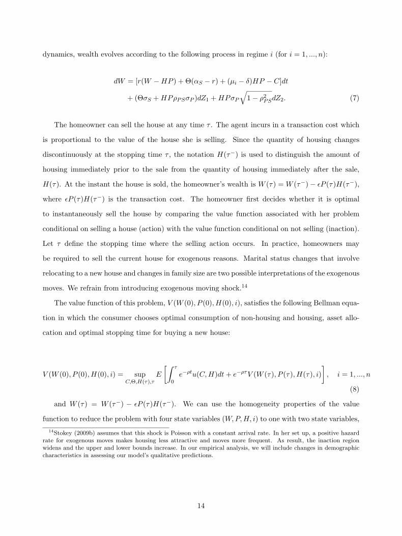
The homeowner can sell the house at any time τ . The agent incurs in a transaction cost which

is proportional to the value of the house she is selling. Since the quantity of housing changes

discontinuously at the stopping time τ , the notation H(τ−) is used to distinguish the amount of

housing immediately prior to the sale from the quantity of housing immediately after the sale,

H(τ). At the instant the house is sold, the homeowner’s wealth is W (τ) = W (τ−)− εP (τ)H(τ−),

where εP (τ)H(τ−) is the transaction cost. The homeowner first decides whether it is optimal

to instantaneously sell the house by comparing the value function associated with her problem

conditional on selling a house (action) with the value function conditional on not selling (inaction).

Let τ define the stopping time where the selling action occurs. In practice, homeowners may

be required to sell the current house for exogenous reasons. Marital status changes that involve

relocating to a new house and changes in family size are two possible interpretations of the exogenous

moves. We refrain from introducing exogenous moving shock.14

The value function of this problem, V (W (0), P (0), H(0), i), satisfies the following Bellman equa-

tion in which the consumer chooses optimal consumption of non-housing and housing, asset allo-

cation and optimal stopping time for buying a new house:

V (W (0), P (0), H(0), i) = supC,Θ,H(τ),τ

E

[∫ τ

0e−ρtu(C,H)dt+ e−ρτV (W (τ), P (τ), H(τ), i)

], i = 1, ..., n

(8)

and W (τ) = W (τ−) − εP (τ)H(τ−). We can use the homogeneity properties of the value

function to reduce the problem with four state variables (W,P,H, i) to one with two state variables,14Stokey (2009b) assumes that this shock is Poisson with a constant arrival rate. In her set up, a positive hazard

rate for exogenous moves makes housing less attractive and moves more frequent. As result, the inaction regionwidens and the upper and lower bounds increase. In our empirical analysis, we will include changes in demographiccharacteristics in assessing our model’s qualitative predictions.

14

z = W/(PH), and i, since

V (W,P,H, i) = H1−γP β(1−γ) V

(W

PH, 1, 1, i

)= H1−γP β(1−γ)v (z, i) . (9)

Furthermore, let c and θ denote the scaled controls c = C/(PH) and θ = Θ/(PH). We refer to

the ratio z as the wealth-to-housing ratio.

A solution consists of a value function v(z, i) defined on the state space, where bounds zi and zi

define an inaction region, z∗i is the optimal regime-dependent return point, and a consumption policy

c∗(z, i) and portfolio policy θ∗(z, i) defined on (zi, zi). The function v(z, i) satisfies the Hamilton-

Jacobi-Bellman equation on the inaction region. Value matching and smooth pasting conditions

hold at the two bounds, and an optimality condition holds at the return point. Compared to

Grossman and Laroque (1990) and Damgaard, Fuglsbjerg, and Munk (2003), the novel feature

exploited here is the Markov chain process governing the dynamics of the expected growth rate of

house prices. Hence, the model features optimal rules that reflect the possibility for the agent to

invest in a different regime of house price growth in the future. The agent has to determine the

optimal rule in each regime, while taking into account the optimal rule in the other one. Thus,

the model generates richer rules than the standard one-regime models. The following proposition

exposes the optimal housing and portfolio choices properties derived from our model.

Proposition 1 The solution of the optimal portfolio choice problem defined above presents the

following properties:

1. v(z, i) satisfies

ρv(z, i) = supc,θ

u(c) +Dv(z, i) +∑j 6=i

λij(v(z, j)− v(z, i))

, z ∈ (zi, zi), (10)

where

Dv(z, i) =((z − 1)(r + δ − µi + σ2P (1 + β(γ − 1)))

+ θ(αS − r − (1 + β(γ − 1))ρPS σSσP )− c)vz(z, i)

+12

((z − 1)2σ2P − 2(z − 1)θ ρPS σPσS + θ2σ2

S)vzz(z, i), (11)

15

v(z, i) = Mi(z − ε)(1−γ)

1− γ , z /∈ (zi, zi) (12)

and Mi is defined as

Mi = (1− γ) supz≥ε

zγ−1v(z, i), (13)

for i = 1, ..., n.

2. The return point z∗i attains the maximum in

v(z∗, i) = Miz∗(1−γ)i

1− γ , for i = 1, ..., n. (14)

3. Value matching and smooth pasting conditions hold at the two thresholds (zi, zi)

v(z, i) = Mi(zi − ε)(1−γ)

1− γ , (15)

vz(z, i) = Mi(zi − ε)−γ , (16)

for zi = zi, zi and i = 1, ..., n.

4. In a state z, where v(z, i) > Mi(z−ε)1−γ

1−γ , the agent chooses a optimal consumption c∗(z, i) and

portfolio θ∗(z, i) and b∗(z, i)

c∗(z, i) =(vz(z, i)β

)1/(β(1−γ)−1)

, (17)

θ∗(z, i) = −ω vz(z, i)vzz(z, i)

+ρPSσPσS

(z − 1), (18)

b∗(z, i) = 1− (1 + θ∗(z, i))/z, (19)

for i = 1, ..., n, and the constant ω is defined as ω = [αS − r + (1− β(1− γ))ρPSσP ] /σ2S.

The main model implications that are tested and analyzed in the empirical part of this paper

are summarized by the following statements:

1. There exists an inaction region for housing, that is, households do not trade housing contin-

uously. Instead, they wait until their wealth is high (low) enough to increase (decrease) their

16

housing assets. The inaction region is limited by a lower bound zi and an upper bound zi in

each regime i, such as zi < zi for i = 1, ..., n.

2. The upper and lower bounds are not constant, but depend on the regime i. In particular, both

the upper and lower bounds in periods of high house price growth are below the respective

bounds in low-growth periods. With higher mean growth rates, the optimal housing holdings

are substantially higher and hence the inaction region is narrower.

3. The portfolio choices of households θ∗(z, i) and b∗(z, i) depend on their individual value of z,

which in turn depends on the regime i. Regarding the risky asset position, the model predicts

the following linear relation between asset holdings and the ratio z of total wealth to housing

wealth when the ratio z is very close to the bounds zi and zi:

θ∗(z, i) ≈ −ωγz +

ρPSσPσS

(z − 1). (20)

The equality holds when z = zi or z = zi. In either case, equation (18) becomes the linear

portfolio rule in Merton (1969), which is equivalent to the equality in (20). The first term

on the right-hand side of (18) becomes “less linear” the further z is from z = zi and z = zi,

because the coefficient of the relative risk aversion varies with z. The lower relative risk

aversion when z is close to the upper or lower bounds leads to higher fractions of wealth

invested in the risky asset than when z is in the center of the inaction region. The second

term is a hedging term. The effect of the hedging term mainly depends on the correlation

between housing and equity return and on the term z − 1. This latter corresponds to the

liquid wealth-to-housing ratio, (B + Θ)/(PH). When the correlation between housing and

equity returns is positive (negative), the stock market position decreases (increases) to the

point where financial wealth-to-housing ratio is null and then increases (decreases).

Figure 4 illustrates the implications of transaction costs, and predictability in housing returns

in a 2-regime set up. In this case, the expected housing return can be high (regime 1) or low (regime

2). Consider that an agent has a ratio of total wealth, W , to housing wealth, PH equal to 2.5 at the

initial time t = 0. Assume that t = 0 belongs to a time interval in which the growth of house prices

is high. The agent must pay a transaction cost every time she adjusts her housing consumption;

17

therefore, she does not move to a more expensive house until she has not accumulated a sufficient

amount of wealth to compensate this transaction cost. When the wealth-to-housing ratio, W/(PH)

in the figure, reaches the upper bound, the agent sells her house and purchases a more expensive one

in order to reset her wealth-to-housing ratio to its optimal level. In Figure 4, this event corresponds

to point 1 at time t = τ1. As a result, the ratio W/(PH) returns to the optimal level z∗h, which

corresponds to point 1∗. Now assume that the economy moves towards a regime of low growth in

house prices shortly after τ1. Note that both the upper and lower bounds in this period of low house

price growth are higher than their respective bounds in the period of high growth. The wealth-to-

housing ratio evolves over time until it hits the upper bound again (point 2) at time t = τ2. Hence,

the agent purchases a more expensive house (point 2∗). At time t = τ3 there is a shift to the regime

of high expected growth in house prices (point 3). As a result, the upper bound shifts down and

the agent moves to a more expensive house (point 3∗), which is bigger than in the regime of low

expected growth in house prices. The example continues with symmetrical situations in which the

agent moves to a less expensive house when her ratio reaches the lower bound (points 4, 5, and 6).

The previous hypothetical example provides insights into the paper’s main contributions: (i) the

portfolio choice implications of three of the main characteristics of housing (i.e. housing being a

durable consumption good as well as an investment asset, high transaction costs, and predictability

in housing returns); (ii) the testable implications of the wealth-to-housing ratio for households that

want to change their housing holdings; and (iii) the testable implications about the overall portfolio

allocation.

[INSERT FIGURE 4 HERE]

Predictability in housing returns implies a time-varying inaction region as the bounds shift

over time adding a second state variable to the GL framework, where housing adjustment occurs

only when the wealth-to-housing ratio hits a time-invariant bound. In addition to the wealth-to-

housing ratio, the time-varying expected growth rate of house prices also determines the optimal

timing for re-balancing the wealth composition.15 The time-varying expected growth rate of house

prices causes a shift in the location of the bound where it is optimal to pay the transaction costs

for re-sizing the housing holdings. The intuition is as follows. When the expectations of house15In Grossman and Laroque (1990), the only state variable is the wealth-to-housing ratio.

18

appreciation are higher, the agent expects to have a lower wealth-to-housing ratio in the next time

period due to a regime switch, therefore, she upgrades to a more expensive house even with a

relatively lower wealth. On the other side, in times of lower expectations of appreciation, the agent

prefers to wait longer until her own wealth increases in order to upgrade to a more expensive house.16

Hence, our framework generates richer portfolio rules than the GL framework. In particular, risk

aversion is also regime-dependent, generating a different portfolio allocation rule for each regime.

The portfolio allocation rule reflects the possibility of regime switches in the future. Therefore, the

agent has to determine the portfolio rule in each regime, while accounting for the possibility of a

future shift in the expected growth rate in house prices.

5 Numerical Simulations

It is not possible to find properties of the portfolio choice problem in closed-form when we take

into account transaction costs. Consequently, we implement an iterative procedure to find the

numerical solution for the problem. A detailed description of this iterative procedure can be found

in Appendix A.2.

Table 3 reports the model’s parameters. We assume a curvature of the utility function of 2 and

a rate of time preference of 2.5%. The parameter 1−β measures how much the agent values housing

consumption relative to the numeraire consumption. It is set at 0.4, which is consistent with the

average proportion of household housing expenditure in the U.S.17 We assume that the risk-free rate

is equal to 1.5% annually. Using U.S. data over the period 1889−2005, Kocherlakota (1996) reports

an average real return on a market index of 7.7% and a standard deviation of 16.55%. We consider

that the estimated house price standard deviation, σP , of 4.47% is too low (see Tables 1 and 2),

due to the inertia in house price indexes. Instead, we assume a house price standard deviation of

10%. This is close to that estimated by Campbell and Cocco (2003) and Landvoigt, Piazzesi, and

Schneider (2011). Campbell and Cocco (2003) report a house price standard deviation of 11.5%,16Davis, Lehnert, and Martin (2008) document that almost all of the decline in the rent-price ratio is attributable

either to a steep decline in risk premium or an increase in the expected growth of house prices, or some combination ofthese two factors. Fillat (2009) presents evidence of a small predictable component in the growth of housing services,which is a proxy for the growth in rents. This alone does not explain entirely the mean reversion of rent-price ratiosafter a shock. Therefore, the absence of a full explanation in the rent growth motivates the presence of predictabilityin housing returns.

17While Cocco (2005) sets 1− β at 0.1, Yao and Zhang (2005) assume that 1− β equals 0.2.

19

using house price data from the PSID for the period 1970 through 1992. Landvoigt, Piazzesi, and

Schneider (2011) report a house price standard deviation of 10%, using micro-data on the San

Diego Metro area for the period 1997 through 2008. We set the correlation coefficient ρPS at 0.25.

We assume that the cost of selling a house is 5% of the unit’s value. This figure includes the

agent’s commissions, legal fees, time cost of searching and the direct cost of moving the consumer’s

possessions. Following previous literature, we set the housing’s physical depreciation rate at 2%

per annum.

[INSERT TABLE 3 HERE]

Figures 5 and 6 are key for showing the three main implications of the model that arise from

Proposition 1 and are tested in the empirical section of the paper. Figure 5 displays the difference

between the value function, v(z(t), i), and the value of changing housing consumption, (z(t) −

ε)1−γMi/(1− γ), against the value of the wealth-to-housing ratio, z(t), using the parameter values

reported on Tables 1 and 3. If this difference is positive, then the agent does not move to a more

or less expensive house. The agent only moves when this difference is zero, that is, when the

value function from not moving given by v(z(t), i) is equal to the value from moving given by

(z(t)− ε)1−γMi/(1− γ).18 Thus, agents only move in two situations: (i) when their total wealth is

high enough relative to their current house’s value so that z(t) reaches the upper bound zi; or (ii)

when their house’s value is too high relative to the total wealth and z(t) reaches the lower bound

zi. The inaction region is limited by a lower bound zi and an upper bound zi in each regime i, such

as zi < zi for both the high regime (i = h) and the low regime (i = l). In Section 7.1, we will test

the existence of the upper and lower bounds hypothesis and we will study its main implications.

[INSERT FIGURES 5 and 6 HERE]

Figure 5 shows the differences of the solution across regimes. The upper and lower bound are

not constant but depend on the regime i. We obtain that zl = 1.575, zl = 6.739, and the ratio

chosen when a new house is purchased z∗l = 3.870 for the low regime. Equivalently, we find that

18This is equivalent to saying that the values of the upper bounds zi and the lower bounds zi are determined bythe value matching conditions (15) for i = h, l, by which the agent is indifferent between not moving and moving.Additionally, the smooth pasting conditions in (16) assure that v(z(t), i) is differentiable on the threshold that triggersthe agent to move. As Figure 5 shows, this implies that v(z(t), i) is less concave than (z(t)− ε)1−γMi/(1−γ) at thesepoints. However, v(z(t), i) must become more concave than (z(t)− ε)1−γMi/(1− γ) somewhere between zi and zi.

20

zh = 0.249, zh = 1.587, and z∗h = 0.491 for the high regime (see Table 4). The economic magnitude

of the calibrated results is sizeable: during a period of low (high) house appreciation, an average

household will decide to buy a more expensive house when the wealth is approximately higher

than 6.7 (1.6) times the value of her current house. On the other hand, when her total wealth is

approximately less 1.5 (0.2) times the value of the house, the agent will engage in a transaction

to buy a less expensive house. Note that: (i) the upper and lower bounds in the high regime are

below their respective upper and lower bounds in the low regime, that is, zh < zl and zh < zl;

(ii) the inaction region for the low regime, [zl, zl], is larger than the inaction region for the high

regime, [zh, zh]; (iii) the inaction regions for the two regimes overlap over a range of z(t) values,

[zl, zh]; (iv) the optimal housing wealth on total wealth, 1/z∗i , for the high (low) regime is 2.035

(0.258), which is lower than the constant ratio of 2.980 (0.340), αh,i, chosen by an agent who faces

no transaction costs;19 and (v) the size of upward adjustment and downward adjustment in a high

regime is lower in than in a low regime, zh − z∗h < zl − z∗l and z∗h − zh < z∗l − zl. In Section 7.2

we will empirically test these types of findings related to the effects of the predictability in housing

returns on the upper and lower bounds.

Figure 5 shows that our framework features a second channel generating a housing transaction:

the regime switching mechanism. A transaction may also occur when the regime switches from high

to low and the agent’s wealth-to-housing ratio z(t) falls within the region [zh = 0.249, zl = 1.575].

Let us assume that z(t) = 0.500. In this case, it is not optimal to sell during the high regime because

her ratio z(t) is not low enough (i.e. z(t) > zh). However, if there is a switch to the low regime,

then the lower bound would increase from zh to zl, and, consequently, it would be optimal for the

agent to sell reduce her housing holdings because z(t) 6 zl. The other interesting case occurs when

there is a regime switch from low to high and z(t) is in the region [zh = 1.587, zl = 6.739].20

As one may expect, this regime-switching mechanism generates rich portfolio rules. The upper

panel of Figure 6 plots the fraction of wealth invested in risky assets against wealth for the two

regimes of expected growth rate of house prices, θ∗(z(t), i)/z(t), for i = h, l. Each curve is drawn19Transaction costs make housing more expensive, so the agent who faced those costs would hold less of her wealth

in the form of housing.20The location of the bounds depends on the transition probabilities to switch regime at the next period given

the current regime. Specifically, for the low regime, the estimated transition probability, λlh, is only about 3.43%,while λhl is about 24.14% for the high regime. As result, the location of the upper bound depends crucially on theprobability of a regime switch from high to low.

21

only for the realizations of z(t) within the inaction bounds. We find that it is optimal to increase

the stock holdings in the low-growth regime and sharply decrease them in the high-growth regime in

order to increase the housing wealth share. Note that the optimal portfolio rules are quite different

from the no transaction costs case, where the fraction of wealth invested in each asset is constant.

What is the channel that drives the agent’s portfolio choices and makes them different from those

provided by other models? The model’s key mechanism is the coefficient of relative risk aversion,

−(z(t)vzz(z(t), i))/vz(z(t), i), which varies with z(t) and with the regime i with i = h, l. As in

Grossman and Laroque (1990) and Damgaard, Fuglsbjerg, and Munk (2003), the lower relative

risk aversion when z(t) is close to either the upper or lower bound leads to higher fractions of

wealth invested in the risky asset than when z(t) is in the inaction region. Then, because the

unconditional probability of switching from a high-growth to low-growth regime is substantial,

λhl = 24.14%, the agent becomes more risk averse where the inaction regions for the two regimes

overlap over a range of z(t) values, [zl, zh]. Therefore, the agent invests less in the stock market

in that region. Hence, the relative risk aversion after a housing trade associated with a high-

growth regime, −(z∗hvzz(z∗h, h))/vz(z∗h, h), is higher than that associated with a low-growth regime,

−(z∗l vzz(z∗l , l))/vz(z

∗l , l). In our benchmark case, we obtain a relative risk aversion of 2.595 for the

high-growth regime and 2.071 for the low-growth regime (see Table 4).

[INSERT TABLE 4 HERE]

Transaction costs also make housing more expensive, so the agent facing those costs holds less

of her wealth in the form of housing. In our benchmark case, due to transaction costs we observe

a reduction of 46% (32%) in housing share in the high-growth (low-growth) regime. In a high-

growth regime the optimal housing holding is substantially higher, the inaction region is narrower

and housing is quite attractive for investment purposes, but transaction costs have the dramatic

effect of lowering the optimal housing wealth to total wealth ratio, 1/z∗i , making the agent more

risk averse after a housing trade. Differently from Grossman and Laroque (1990) and Damgaard,

Fuglsbjerg, and Munk (2003), the coefficient of risk aversion depends on the current regime. In

summary, the model delivers a regime contingent portfolio rule. Additionally, due to the possibility

of a regime change, the portfolio rule optimally reflects the agent’s investment set in the alternative

regime.

22

The lower panel plots the fraction of wealth invested in the risk-free asset, b∗(z(t), i)/z(t). We

find that: (i) the agent is a net borrower in both regimes; (ii) she borrows a bigger amount in the

high-growth regime (to increase her housing holdings, which are more attractive in the high-growth

regime) than in the low-growth regime; and (iii) her borrowing increases with her ratio z(t). In

Section 7.3, we will empirically test these findings related to the portfolio choices of households.

Appendix A.3 presents a sensitivity analysis of the benchmark model.

In Section 3, we provide evidence that the degree of predictability varies across the U.S. census

divisions. The theoretical relevance of the house price dynamics parameters is evident when ana-

lyzing the results of the calibration. Due to the shorter time series and the recent boost episode

(2007− 2010), house prices growth rates are markedly more negative for the U.S. census divisions

than for the U.S. at aggregate level (see Table 1). As result, inaction regions are larger than those

calculated in the benchmark case for the low-growth regime (see Table 4). This boost episode was

preceded by a long period 1998− 2006 in which house prices dramatically appreciated in the New

England and Middle Atlantic (Northeast), South Atlantic (South) and Pacific (West) census divi-

sions. In fact, according to our calibration, we expect these census divisions to be characterized by

markedly lower values of the lower and upper bounds, narrower inaction regions, and lower average

risky stock holdings in the same period. In Section 7.2 and 7.3, we will test these implications

empirically at U.S. state level.21 To capture periods of high house price appreciation at U.S. state

level, we construct a variable that we call “Hot Housing Market Indicator” (HHMI). The HHMI

is function of the estimated smooth probability of being in a period of high growth rate for each

state. This indicator will serve as a proxy for the second state variable of our model.

It is important to recognize that while the optimizing behavior characterized above is that of

a hypothetical agent living infinitely, the data we will use later to test the model’s predictions are

drawn from a cross-section of demographically heterogeneous consumers. Therefore, to assess the

descriptive fit of our model, we will include demographic characteristics and changes in demographic

characteristics, for example, household head age in two age bands, change in marital status and

change in family size, which may absorb determinants other than dynamic variations of the type

featured by our representation of a typical agent’s problem.21Appendix A.4 provides evidence that the degree of predictability varies across the U.S. states.

23

6 Data

To test the theoretical predictions of our model, we use household level survey data from the Panel

of Income and Study (PSID) from 1984 to 2007, and from the Survey of Income and Program

Participation (SIPP) of the U.S. Census Bureau from 1997 to 2005. Both surveys have data on

asset holdings and housing wealth. PSID regularly collects information about home values and

mortgage debt; occasionally, it also collects information about behavior on savings and wealth.

SIPP has a detailed inventory of annual real and financial assets and liabilities. It also contains

more frequent measures of those assets that are relevant for assistance measures since its main

purpose is to evaluate the effectiveness of government transfer programs. PSID is a nationally

representative longitudinal sample of approximately 9, 000 households. At each moment, SIPP

tracks approximately 30, 000 households. During the period considered, information was collected

from three consecutive groups of households that were interviewed during the years 1996 − 2000

(four times), 2001 − 2003 (three times), and 2004 − 2006 (two times), respectively. During its

active period, each panel is interviewed every year, while panels of households do not overlap

across periods. SIPP over-samples from areas with high poverty concentrations, which should be

taken into account when interpreting the results. Its longitudinal features enable the analysis of

dynamic characteristics, such as changes in income and in household and family composition, or

housing dynamics. Its cross-sectional features allow us to keep track of household wealth. Both

surveys allow us to study the empirical implications of the model outlined above. In particular, we

focus on the identification that arises when households sell their current house to buy a new one.

Unfortunately, neither data set offers a measure of overall transaction costs paid by households

when they change their house.

Using the PSID data, we calculate financial wealth as the summation of an individual’s house

value, their second house value (net of debt), business value (net of debt), other assets22 (net of

debt), stock holdings (net of debt), checking and savings balances, IRAs and annuities less the

mortgage principal on the primary residence23, and human capital. We delineate these variables

into those that are considered risky assets and those that are safe assets. The risky assets are

comprised of the stock holdings, IRA and annuity holdings. The safe asset is comprised of other22Other assets include bonds and insurance.23For comparability across waves of surveys, we focus only on the primary mortgage.

24

assets (net of debt), checking and savings balances, less the principal on the primary residence.

Generally, the variables we utilized from the SIPP data set are net of debt, the sole exception is

property value. Using the SIPP data, we calculate risky assets as the summation of equity in stocks

and mutual funds, equity in IRAs, and equity in 401k and thrifts. The safe assets are interest-

earning assets in banks and other institutions less outstanding mortgage balance. The value for

financial wealth is calculated by adding the risky asset value to safe asset value, business equity,

property value of primary residence, housing equity in second residence and other assets. In both

PSID and SIPP data sets, the measure of house value is given by homeowners’ estimate of home

value. Home value is problematic in that there might be a large amount of measurement error in

the figure quoted. However, we would argue that while most homeowners only have a general idea

of the value of their home, owners who are near to the bound or have recently bought a house have

very precise knowledge of the value of their home. Hence, if households do not own risky stock or

safe assets such as checking and savings balances, IRA and annuity holdings, we set these holdings

to zero. In addition, we exclude households whose total reported stockholdings are negative. This

exclusion does not affect the qualitative results reported below.

We calculate the total wealth of each household including unobservable human capital (human

wealth). Following Jagannathan and Wang (1996), we estimate the human capital of each household

as capitalized wage income, that is, as the present value of a growing annuity.24,25

Tables 5 and 6 show the descriptive statistics for the main variables that we use in the empirical

analysis. We present statistics for the full sample and also for the selection of households that moved

to a bigger or a smaller house (second and third pair of columns, respectively.) We show mean and24 We assume that for each household, the wage remains constant at the current real level until age of 65, g = 0%,

and then the wage ends, as in Heaton and Lucas (2000) and Eberly (1994). The stream of labor income cash flows isdiscounted back at a real interest rate of five percent per year, R = 5%. We use the current annual total householdearned income as the cash flow for the annuity CFt. We also assume that households earn income until they retire atthe age of 65. Therefore, we assume that households older than 65 have zero human capital. Under these assumptions,the human capital of each household i of age n (younger than 65 years, that is, n < 65) can be estimated using thefollowing formula:

Li,t =CFtR− g

"1−

»1 + g

1 +R

–(65−n)#. (21)

25As Palacios-Huerta (2003) acknowledges, measuring human capital as capitalized wage income has several limi-tations. First, it does not account for the capital gains of the stock of human capital. Second, this simple measureassumes that labor supply is exogenous. Third, it ignores the worker’s skill premia and experience. Fourth, it doesnot net out the effect of physical capital on labor income and human capital returns. Fifth, this measure does notaccount for regional differences. We have run different robustness checks on these five limitations for all the resultsthat we present. We have found that the results obtained using the measure of human capital in Jagannathan andWang (1996) are robust.

25

standard deviations of the relevant variables. The single most important variable is the wealth-

to-housing ratio, z.26 For the PSID sample, we observe that, on average, the value of the house

is approximately two-thirds of the total household wealth. This average ratio is lower for movers,

not controlling for any other reason to move that is exogenous to the model. Stock holdings are

roughly 10.2% of the financial wealth, and safe assets without debt holdings represent 10.9% of

financial wealth, much higher for households who buy a more expensive house. We also report

statistics on stock holdings that do not take into account the retirement assets’ (IRA, 401k) impact

on financial wealth and on liquid wealth where liquid wealth is total wealth less home equity and

other illiquid assets such as cars. We define the dummy Move big (small) to identify households

selling the current house to buy a more (less) expensive house in the same U.S. census region.

Hence, we report summary statistics for variables that will help us to distinguish between changes

in housing that occur because of reasons that are exogenous to the model and changes in housing

that occur because individuals have a total wealth-to-housing ratio that is close to the boundary.

[INSERT TABLES 5 and 6 HERE]

In order to capture exogenous shocks, we define variables to examine changes in demographics

from the year before to the year after home purchase. ∆ Family size shows the statistics of changes

in family size. ∆ Married is a dummy variable which takes a value of one if the individual gets

married. ∆ Employment is a dummy variable which takes a value of one if the individual changes

her employment status. During the sample period analyzed using the PSID data, the size of the

household (in number of members) decreased by −0.044. The family size increased for movers

to a bigger house, 0.071, while it decreased for movers to a smaller house, −0.235, meaning that

housing consumption is strictly related to the number of members in the household. Marriages

also increase, by almost 1.6%, and again this figure is substantially higher for movers. The mean

age of the household head is 49.09 years. The mean age of movers is shifted towards a younger

population: 40.38 years for household heads moving to a more valuable house and 46.07 years

for household heads moving to a less valuable house. The regional composition, in terms of census

regions are 15.6% Northeast, 26.6% Midwest, 41% South, and 16.9% West. The summary statistics26Although we show statistics for the wealth-to-housing ratio without and with human capital, z and ez, respectively,

we use the measure with human capital in the rest of the paper.

26

using SIPP do not differ substantially. It is worth mentioning the differences in age composition,

where the youngest group is more represented in PSID. In terms of moving, the group of movers to

a bigger and smaller house is lower in SIPP than in PSID in percentage terms, although we have

more observations for this group in SIPP. Geographic composition and other relevant variables are

comparable both in levels, standard errors, and also conditional on moving household.

Table 7 provides information on the percentage of movers by current ownership status (owner,

renter, or occupied) over total households in the PSID and SIPP surveys across all years. The four

columns represent the percentage of households that moved to a new address, that moved to a new

address in the same U.S. macro region, that moved to a new address in the same U.S. state, and

that moved to a new address and were previously not homeowners. While we can easily identify

movers in PSID because it reports explicitly whether there has been a move since the previous

interview, we have to identify movers in SIPP keeping track of the households’ address identifier.

That identification mechanism is what generates differences between SIPP and PSID that were not

present in Tables 5 and 6. In the upper panel of Table 7, we observe that the percentage of owners

who move is much lower than the percentage of renters, who have a much higher mobility than

owners. The percentage of movers to a different U.S. census region or U.S. state is very low among

owners. The total inflow of homeowners is different between PSID and SIPP. While households

in SIPP entering in home ownership during the sample is 5.47%, more than half of the movers in

PSID are new homeowners.27 Despite reporting data for renters, it is necessary to emphasize that

we do not model renters’ decisions. Our agent does not have the possibility of renting. In order to

consume housing services, the only option is to pay a transaction cost and purchase a new house

and derive a flow of services from it. Renting is not part of the model and we select the sample of

homeowners only. Therefore, the model is mute about the renters who moved during the sample

period.

[INSERT TABLE 7 HERE]27New in the sense that they did not own at t− 1 but it could be the case that they were owners in the past.

27

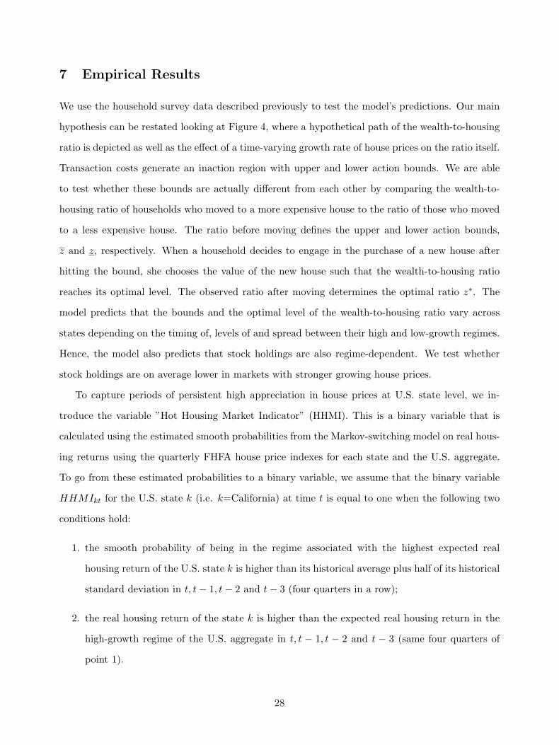
7 Empirical Results

We use the household survey data described previously to test the model’s predictions. Our main

hypothesis can be restated looking at Figure 4, where a hypothetical path of the wealth-to-housing

ratio is depicted as well as the effect of a time-varying growth rate of house prices on the ratio itself.

Transaction costs generate an inaction region with upper and lower action bounds. We are able

to test whether these bounds are actually different from each other by comparing the wealth-to-

housing ratio of households who moved to a more expensive house to the ratio of those who moved

to a less expensive house. The ratio before moving defines the upper and lower action bounds,

z and z, respectively. When a household decides to engage in the purchase of a new house after

hitting the bound, she chooses the value of the new house such that the wealth-to-housing ratio

reaches its optimal level. The observed ratio after moving determines the optimal ratio z∗. The

model predicts that the bounds and the optimal level of the wealth-to-housing ratio vary across

states depending on the timing of, levels of and spread between their high and low-growth regimes.

Hence, the model also predicts that stock holdings are also regime-dependent. We test whether

stock holdings are on average lower in markets with stronger growing house prices.

To capture periods of persistent high appreciation in house prices at U.S. state level, we in-

troduce the variable ”Hot Housing Market Indicator” (HHMI). This is a binary variable that is

calculated using the estimated smooth probabilities from the Markov-switching model on real hous-

ing returns using the quarterly FHFA house price indexes for each state and the U.S. aggregate.

To go from these estimated probabilities to a binary variable, we assume that the binary variable

HHMIkt for the U.S. state k (i.e. k=California) at time t is equal to one when the following two

conditions hold:

1. the smooth probability of being in the regime associated with the highest expected real

housing return of the U.S. state k is higher than its historical average plus half of its historical

standard deviation in t, t− 1, t− 2 and t− 3 (four quarters in a row);

2. the real housing return of the state k is higher than the expected real housing return in the

high-growth regime of the U.S. aggregate in t, t − 1, t − 2 and t − 3 (same four quarters of

point 1).

28

The HHMI is based on these two conditions because they embed two specific pieces of information.

The first condition captures the likelihood that there has been a regime switch in the U.S. state k

based on a turning point probability. We define the turning point probability when the estimated

smooth probability reaches a 90% statistical level. The logic underlying the first condition is to

detect whether a housing market peak relative to its historical average in the state k has been

reached and it has lasted at least four quarters in a row. Hence, condition 1 allows us to classify

states’ house prices according to the degree of cyclicality in their real housing returns.28 The

second condition verifies whether the real housing return in the state k is substantially high when

compared to the overall U.S. housing market. Appendix A.4 provides a detailed description of this

estimation and the results.

7.1 Existence of the Upper and Lower Bounds Hypothesis

The first hypothesis to be tested is the existence of the optimal upper and lower bounds provided

by the model in the cases in which transaction costs are taken into consideration. Specifically,

Hypothesis 1. zi < zi. Therefore, z is significantly different (and lower) from z for a given

expected growth rate in house prices in regime i.

This hypothesis states that the ex-ante average value for the ratio of total wealth-to-housing

holdings zit for households who own a house and move to a less expensive one z is significantly

different (and lower) from the ratio of total wealth to housing holdings for households who own a

house and move to a more expensive one z.

To test this hypothesis, we estimate the following reduced-form model, which exploits the

variation across households and years:

zit = γ0 + γ1 ·mBIGit + γ2 ·mSMALLit + Γ ·Xit + uit, (22)

where zit is the total wealth-to-housing ratio of household i at time t; mBIGit is a binary variable

28The condition that the smooth probability of being in the regime associated with the highest expected realhousing return reaches the turning point probability is satisfied in some periods by states such as California andFlorida in which housing markets experienced a particularly high appreciation in the same periods. Hence, theseperiods are generally characterized by high and pronounced appreciation in house prices. Differently, condition 1is not satisfied by states such as Alabama and Montana whose housing markets have experienced prolonged andcontinuous high-growth phases that are mainly characterized by modest growth in house prices.

29

equal to one if the household is increasing its housing holdings (i.e. moving to a more expensive

house); mSMALLit is a binary variable equal to one if the household is decreasing its housing holdings

(i.e. moving to a less expensive house); Xit contains a set of control variables that intend to capture

changes in housing due to exogenous causes, unrelated to the total wealth-to-housing ratio, and

uit is an error term. The set of controls in Xit includes changes in employment status, changes in

family size, changes in marital status, and age controls. All variables control ex-ante changes to

examine changes from the year before to the year after home purchase. The regression omits the

households who do not move, treating them as a benchmark. Therefore, we check whether γ1 is

significantly positive and different from zero, which means that the total wealth-to-housing ratio of

the households who move to a more expensive house is significantly higher than the ratio of those

who do not move. We run the pooled regression in equation (22) with year fixed effects and also

separate regressions for each year.

[INSERT TABLES 8 AND 9 HERE]

The results of testing the first hypothesis are shown in Tables 8 and 9. The first column shows

the results for the pooled regression with year fixed effects. It shows that the average value of zit

for families that do not move, γ0, is 2.166 for PSID and 3.471 for SIPP. It is worth pointing out

that the total wealth of the total wealth-to-housing ratio includes the human capital as calculated

in Section 6. The ex-ante average value of zit for households that moved to a bigger house is 2.456

for PSID and 1.677 for SIPP above the non-movers average with a 99% significance for PSID and

SIPP, respectively. Similar results are obtained when running yearly regressions. Note that γ2 is

not significantly different from γ0 for PSID, but it is for SIPP. Thus, the average total wealth-

to-housing ratio zit for non-movers is not significantly different from the ratio for movers to less

expensive houses. It can be inferred that the distribution of the total wealth-to-housing ratio is

skewed to the left and on average, agents are closer to moving down according to our model. We

also run a test on the coefficients γ1 and γ2 being equal, which is strongly rejected for most of the

years. This result supports the obvious hypothesis of the existence of the inaction region in the

presence of transaction costs since the test shows that the upper and lower bounds are significantly

different from each other. The results of the test also show evidence that the ratio zit is time-

varying, on average. This is a clear effect for non-movers and for households who move to a more

30

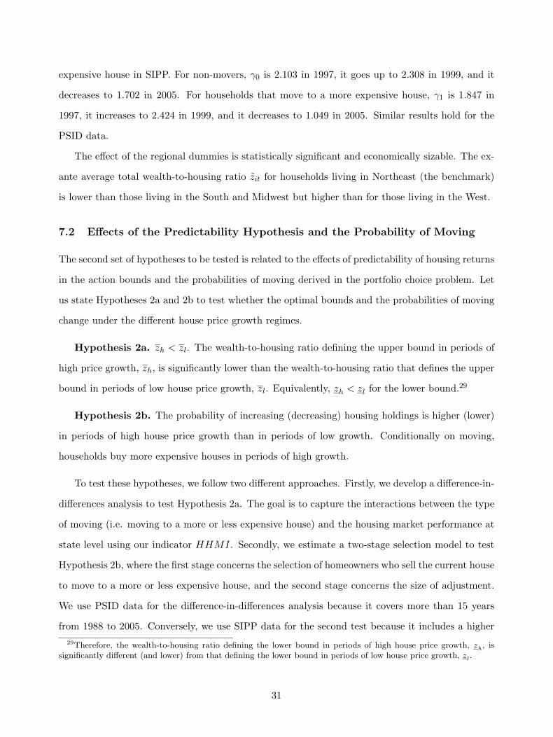
expensive house in SIPP. For non-movers, γ0 is 2.103 in 1997, it goes up to 2.308 in 1999, and it

decreases to 1.702 in 2005. For households that move to a more expensive house, γ1 is 1.847 in

1997, it increases to 2.424 in 1999, and it decreases to 1.049 in 2005. Similar results hold for the

PSID data.

The effect of the regional dummies is statistically significant and economically sizable. The ex-

ante average total wealth-to-housing ratio zit for households living in Northeast (the benchmark)

is lower than those living in the South and Midwest but higher than for those living in the West.

7.2 Effects of the Predictability Hypothesis and the Probability of Moving

The second set of hypotheses to be tested is related to the effects of predictability of housing returns

in the action bounds and the probabilities of moving derived in the portfolio choice problem. Let

us state Hypotheses 2a and 2b to test whether the optimal bounds and the probabilities of moving

change under the different house price growth regimes.

Hypothesis 2a. zh < zl. The wealth-to-housing ratio defining the upper bound in periods of

high price growth, zh, is significantly lower than the wealth-to-housing ratio that defines the upper

bound in periods of low house price growth, zl. Equivalently, zh < zl for the lower bound.29

Hypothesis 2b. The probability of increasing (decreasing) housing holdings is higher (lower)

in periods of high house price growth than in periods of low growth. Conditionally on moving,

households buy more expensive houses in periods of high growth.

To test these hypotheses, we follow two different approaches. Firstly, we develop a difference-in-

differences analysis to test Hypothesis 2a. The goal is to capture the interactions between the type

of moving (i.e. moving to a more or less expensive house) and the housing market performance at

state level using our indicator HHMI. Secondly, we estimate a two-stage selection model to test

Hypothesis 2b, where the first stage concerns the selection of homeowners who sell the current house

to move to a more or less expensive house, and the second stage concerns the size of adjustment.

We use PSID data for the difference-in-differences analysis because it covers more than 15 years

from 1988 to 2005. Conversely, we use SIPP data for the second test because it includes a higher29Therefore, the wealth-to-housing ratio defining the lower bound in periods of high house price growth, zh, is

significantly different (and lower) from that defining the lower bound in periods of low house price growth, zl.

31

number of households who sell the current house to move to a more or less expensive house.

7.2.1 Does predictability affect the action bounds? Difference-in-differences analysis

Let us consider the following reduced form model:

zit =γ0 + γ1 ·HHMIkt + γ2 ·mBIGit + γ3 ·mSMALLit

+ γ4 ·mBIGit ×HHMIkt + γ5 ·mSMALLit ×HHMIkt + Γ ·Xit + uit, (23)

where zit is each household i’s ex-ante value for the total wealth-to-housing ratio. As in the previous

subsection, mBIGit is a binary variable equal to one if the household is moving to a house with a

higher value than that currently owned, while mSMALLit is equal to one if the household moves to

a house with a lower value than that currently owned. Then, we interact HHMIkt with mBIGit

and mSMALLit . In this regression, we include the same control variables listed above.

The hypothesis test consists of a difference-in-differences analysis. Table 10 reports its results.

We choose households that did not move in cold years, HHMIkt = 0, as the control group.

The positive sign in γ1 shows that households that moved big (increased her housing holdings)

had a 3.186 higher zit than households that did not move in a cold year. The negative sign in

the coefficient γ3 confirms that the total wealth-to-housing ratio, on average, is 1.030 lower in hot

markets than in cold markets. The main results of this specific analysis arise from the terms in which

we interact mBIGit with HHMIkt and mSMALLit with HHMIkt. The term mBIGit × HHMIkt

captures the difference between the following two terms: (i) the difference between the average

zit for the upper boundary in cold and hot years; and (ii) the difference between the average zit

for non-movers in cold and hot years. The negative sign in the coefficient γ4 indicates that the

decrease in zit in the upper boundary in the transition from cold to hot markets is lower than the

decrease in zit for non-movers in the transition from cold to hot markets. However, the coefficient γ5

associated with mSMALLit×HHMIkt is not significant. These empirical results confirm the model’s

implications in the sense that housing return predictability affects the total wealth-to-housing ratio

and hence the upper bounds suggesting that the inaction region changes over time. Our estimate

associated with the lower bounds, γ2, is not correctly signed and insignificant. These results are

consistent with those obtained in the previous test for PSID. Consequently, the empirical results are

32

significant and the coefficients of the control variables are consistent with our previous empirical

analysis. Moreover, the regional analysis shows that, compared to the Northeast (benchmark

region), households in the Midwest and South present higher total wealth-to-housing ratios and

households in the West present lower ratios.

[INSERT TABLE 10 HERE]

7.2.2 Does predictability affect the probability of moving and the size of adjustment?

A two-stage selection model

To answer this question, we follow Bertola, Guiso, and Pistaferri (2005) and we implement the

selection model introduced by Heckman (1979). We will focus our empirical approach on effects

of housing return predictability on the frequency and width of upward and downward adjustment

(i.e. increasing or decreasing their amount of housing holdings). We let the upward and downward

adjustment of the current housing stock occur when a latent variable D∗i = X′itϕ + uit, is driven

to be larger than zero. The assumption that the error term uit is normally distributed yields the

probit model:

Pr(D∗i > 0) = φ(X′itϕ), (24)

where Xit is a vector of variables and φ(X′itϕ) is the standard normal cumulative density function

evaluated at X′itϕ. In our framework, such a latent variable is interpreted as the distance between

the total wealth-to-housing ratio, z, and the optimal return point, z∗. The model predicts that

upward (downward) adjustment is more (less) likely to be observed, for a given z, when house

prices experience high appreciation. We re-introduce our indicator HHMI to capture periods of

persistent high house price growth in the state where the households live. In practice, households

can sell the current house located in a state and buy a more (less) expensive house in another state.

Hence, it would be also important to control for the level of house prices in the state where the

household is moving to. This latter variable should affect the likelihood and the size of housing

adjustment. However, this exclusion does not affect the qualitative results reported below because

we are considering households selling the current house to buy a bigger one in the same U.S. census

macro-region and the percentage of movers to a different state is substantially low among owners

33

(see Table 7).30 Columns 1 and 3 of Table 11 report marginal effect estimates from the probit

regressions for increasing and decreasing the amount of housing holdings. After controlling for

observable characteristics, the probability of upgrading (downgrading) increases (decreases) with

the value of the total wealth-to-housing ratio, zit. Consequently, our second state variable HHMIkt

affects positively (negatively) the probability of an upgrading (downgrading) as predicted by our

theoretical model. Both coefficients are highly statistically significant and economically important.

In addition, households living in the West are more likely to upgrade and downgrade and the

economic effect is also substantial.

The probit regression is the first step for testing Hypothesis 2b. Our model also delivers sign

predictions for the size of the adjustment conditional on adjusting. It predicts that persistent

higher growth in house prices decreases the size of the adjustment. However, the disturbance of

the regression equation for the size of the adjustment depends upon unobserved heterogeneity. We

treat the problem adopting Heckman’s selectivity corrections in the regression. We use the value of

zit prior to adjustment as a selection variable because theory predicts that it affects the likelihood

of adjusting but not the size of adjustment if it occurs. Following Bertola, Guiso, and Pistaferri

(2005), we use as independent variable the log of the adjustment, ln(z − z∗) for upgrading and

ln(z∗−z) for downgrading.31 The results of the second stage of the Heckman selectivity regressions

are reported in Columns 2 and 4.32 The most important effect is captured by the variable HHMIkt.

The effect is statistically significant and economically sizable when households sell the current house

to buy a more expensive house. It implies that the distance between the upper bound zi and the

optimal adjustment point z∗ is lower in periods of persistent high growth in house prices. In the

downward case, the coefficient associated with HHMIkt is not significant but it points in the right

direction.30In our setup, we refrain from introducing the option of selling the house at the price P in the household’s current

market and buying a more or less expensive one at the price P ′ in the region to which the household relocates in thenext move. In this setup, the household’s indirect utility depends on six state variables, V (W,P,H, P ′, j, k), where jis the regime (i.e. high or low) characterizing house price P , while k is the regime (i.e. high or low) characterizinghouse price P ′. A similar model without house return predictability is analyzed by Flavin and Nakagawa (2008).

31In the second stage, we do not include households who sell the current house to buy a more (less) expensivehouse but whose total wealth-to-housing ratio increases (decreases) between the two purchases. We have two possibleexplanations. The first is that total wealth is not following the continuous diffusion process assumed by our modelbut rather positive or negative jumps may be occurring in the total wealth process. The second is that total wealthmight be affected by a measurement error.

32We implement a standard GLS procedure to calculate appropriate standard errors for the estimated coefficients(see Greene (2008)).

34

[INSERT TABLE 11 HERE]

7.3 Portfolio Choice Hypothesis

Do households hold more risky stock before moving to a bigger house? To answer this question,

we develop the following test, in which we study the holdings of risky securities relative to wealth

and their link to the decision to buy a more or less expensive house.

Hypothesis 3. ΘmBIG/Wit > Θit/Wit. Therefore, the risky assets holdings relative to the

financial wealth before moving to a bigger house, ΘmBIG/Wit, is significantly different (and higher)

from the average risky assets holdings relative to the financial wealth of households who do not

move, Θit/Wit.

To test Hypothesis 3, we estimate the following reduced form model:

Θit

Wit= γ0 + γ1 ·mBIGit + γ2 ·mSMALLit + Γ ·Xit + uit. (25)

The results of the test of Hypothesis 3 are shown in Tables 12 and 13. We run the pooled

regression with year fixed effects and also year by year. The first column shows the results for the

pooled data. It shows that the average holdings of risky stock on financial wealth for non-movers is

8.1% for PSID data and 9.7% for SIPP data. The average holdings of risky stock relative to financial

wealth for households that moved to a more expensive house is 3% higher, that is 11.1%. For SIPP

movers to a more expensive house the risky holdings account for 13.8% of their financial wealth.

Looking at the coefficients year by year in the subsequent columns, we observe that the average

holdings of risky stock for non-movers is in the range [5%, 19.7%] for PSID and [13.7%, 15.7%] for

SIPP. In sum, households that move to more expensive houses have higher risky asset holdings.33

[INSERT TABLES 12 and 13 HERE]

In order to test the effect of housing return predictability on risky stock holdings, we follow

Chetty and Szeidl (2011). They use SIPP data to estimate the causal effect of house value on33Uncertainty around the estimates for the lower bound does not allow us to make a statement about how the level

of risky assets in that an investor who has just moved to a less valuable house should have in her portfolio, althoughwe observe that households holds less risk stock before moving to a less expensive house. Only the negative andsignificant sign for γ2 in the pooled regression using SIPP data (shown in Table 13) indicates that agents moving toa smaller house hold less risky stock than non-movers and agents moving to a bigger house.

35

portfolio allocations. They provide evidence that an increase in housing holdings substantially

reduces the amount households invest in risky stocks. Our model provides an additional implication:

Hypothesis 4. Θ(high)it/Wit < Θ(low)it/Wit. On average, households should hold less risky

stock holdings in a period of high house appreciation.

To test this hypothesis, we follow the empirical strategy developed by Chetty and Szeidl (2011)

and we extend it to account for housing return predictability. Their goal is to estimate the effect

of owning a more expensive house on portfolio choice. Because both portfolio and housing are

endogenous choices that are affected by unobserved factors such as background risk (see Cocco

(2005) and Davidoff (2010)), previous empirical work (see Heaton and Lucas (2000), Yamashita

(2003) and Cocco (2005)) could document the cross-sectional correlation between house values and

portfolio choices but they couldn’t identify the casual effect of housing on portfolios.

Chetty and Szeidl (2011) highlight that the key to capturing the effects of housing on portfolio

is to distinguish between changes in mortgage debt and changes in home equity wealth. Because

property value is the sum of mortgage debt and home equity, changes in property value should

reduce the stock share of liquid wealth through the combination of these two components, but

home equity increases stock holdings through a wealth effect.34 To characterize the effect on

housing return predictability on stock holdings, we include our indicator HHMIkt and we interact

HHMIkt with house value and home equity to estimate a specification analogous to that discussed

in Chetty and Szeidl (2011):35

Θit

Wit

= γ0 + γ1 · house valueit + γ2 · home equityit + γ3 ·HHMIkt

+ γ4 · house valueit ×HHMIkt + γ5 · home equityit ×HHMIkt + Γ ·Xit + uit, (26)

34Chetty and Szeidl (2011) exploit two instruments to generate variation in home equity and property value: theaverage house value in the state where the household lives in the current year and the average house value in thestate in the year that the household bought the house. Because SIPP data contain information on households whopurchase houses in different years and observe portfolio allocations in different years in states, they include state,current year, year of house purchase and age fixed effects in the regression specification below. In addition, we includea 10-piece linear spline for liquid wealth, income, and number of children under 15.

35Our specification is similar to that used by Chetty and Szeidl (2011) to examine how the effect of housing onportfolios covaries with the volatility of local housing markets (see Section 4.3 and Table 7 of their paper). To testwhether the effects of housing on portfolios differ in high versus low-risk environments, they interact a high-riskindicator with property value and home equity. The high-risk indicator is equal to one when the standard deviationof annual house price growth rates using the OFHEO data by state is above the median volatility of 4.5%.

36

where Θit/Wit is the risky share of liquid wealth. Because we do not have information on the risk

characteristics of retirement portfolios in SIPP, we follow Chetty and Szeidl (2011) and we do not

include retirement assets (i.e. IRA and 401K) in the risky stock holdings in this specification. The

error term of this regression might capture other sources of heterogeneity in portfolios, including

background risk (see Heaton and Lucas (2000)), heterogeneity in risk aversion, or measurement

error. To address this concern, we also instrument the house value and home equity using the state

price index in the year of home purchase and the state price index at time t.

Table 14 reports the results. Columns 1-4 report first stage regressions and Columns 5 and 6

report the two-stage least square estimates.36 The coefficient estimates in Column 5 imply that

a $100, 000 increase in property value reduces the risky share of liquid wealth approximately by

2.2%, while a $100, 000 increase in home equity increases it by 3%. The coefficients point in the

right directions but they are statistically insignificant. The coefficient on the interaction between

home equity and HHMIkt is −2.7% and is statistically significant. Hence, consistent with model

predictions, housing has a substantial and significant effect on stock holdings during a period of high

house appreciation. Column 6 replicates the specification in Column 5 but replaces the dependent

variable with an indicator for owning stocks. Consistent with the stock share results, housing has

an effect on stock market participation and has a differential effect in low- and high-growth states.

[INSERT TABLE 14 HERE]

8 Conclusions

As the recent literature on portfolio choice models with real estate has emphasized, there are

important frictions in the housing markets that affect agents’ portfolio decisions. For instance,

models have considered housing as a durable consumption good as well as an investment asset,

or the existence of large transaction costs in housing markets. This paper makes progress in this

direction by studying an empirically relevant model that includes predictability in housing returns.

First, we study the existence of predictability in housing returns and we find that the dynamics

of housing prices are well captured by a Markov switching model. The recent steep rise of U.S.36The number of observations is lower compared to the previous analysis. Each observation in the cross-sectional

sample is for a unique household. As in Chetty and Szeidl (2011), we only use data from the first year in whichportfolio allocations and house values are observed.

37

house prices has received a lot of attention in the media and in the literature, but one interesting

feature of our analysis is that it documents substantial differences in expected growth rates, spread

between highest and lowest growth rates, and timing across U.S. census divisions and U.S. states

during the same period. Part of these variations may stem from institutional differences across

U.S. states. However, in future work, it would be interesting to study and model the determinants

of the distribution of house prices.

Moreover, we set up and solve a novel model for studying how housing return predictability

affects housing consumption and portfolio choices. We find that households consider two state

variables for making their decisions under predictability in housing returns and transaction costs:

the wealth-to-housing holdings ratio and the time-varying mean rate of house price growth. As

in the GL model, agents increase (decrease) their housing asset holdings only when their wealth-

to-housing ratio reaches an optimal upper (lower) bound; consequently, they do not trade housing

when their wealth-to-housing ratio is between the upper and lower bounds. One of the main

contributions of our model is to show that these bounds are time-varying and decrease when house

prices are expected to rise, that is, the bounds are low in periods of high growth in housing prices

and high in periods of low growth. We also show that relative risk aversion is different in high

and low-growth regimes, which explains the differences in optimal portfolio choices between both

regimes.

Finally, we use PSID and SIPP data to test whether the upper and lower inaction bounds

are affected by housing return predictability at U.S. state level. Our empirical results show that

the high growth in house prices in some U.S. states experienced during the period 1998 − 2006

affected the likelihood of housing purchase and increased the investment in housing. Our analysis

also suggests that the current downturn of house prices and the substantial amount of mortgage

debt can dramatically increase the illiquidity of housing as many households postpone selling their

houses. In future work, it would be interesting to explore such interactions when new PSID and

SIPP data become available.

38

References

Ang, A., and G. Bekaert. 2002. “International Asset Allocation with Regime Shifts.” Review of

Financial Studies 15 (4): 1137–1187.

. 2007. “Stock Return Predictability: Is It There?” Review of Financial Studies 20 (3):

651–707.

Ang, A., and A. Timmermann. 2011. “Regime Changes and Financial Markets.” Working paper

17182, National Bureau Economic Research.

Attanasio, O. 2000. “Consumer Durables and Inertial Behaviour: Estimation and Aggregation

(S,s) Rules for Automobile Purchases.” Review of Economic Studies 67 (4): 667–696.

Baele, L. 2005. “Volatility Spillover Effects in European Equity Markets.” Journal of Financial

and Quantitative Analysis 40 (2): 373–401.

Barberis, N. 2000. “Investing for the Long Run When Returns are Predictable.” Journal of

Finance 55 (1): 225–264.

Bertola, G., L. Guiso, and L. Pistaferri. 2005. “Uncertainty and Consumer Durables Adjustment.”

Review of Economic Studies 72 (4): 973–1007.

Brennan, M., E. Schwartz, and R. Lagnado. 1997. “Strategic Asset Allocation.” Journal of

Economic Dynamics and Control 21 (8-9): 1377–1403.

Campbell, J. Y., and J. F. Cocco. 2003. “Household Risk Management and Optimal Mortgage

Choice.” Quarterly Journal of Economics 118 (4): 1449–1494.

Campbell, J. Y., S. Giglio, and C. Polk. 2010. “Hard Times.” Working paper 16222, National

Bureau Economic Research.

Campbell, J. Y., and R. J. Shiller. 1988. “The Dividend-Price Ratio and Expectations of Future

Dividends and Discount Factors.” Review of Financial Studies 1 (3): 195–228.

Campbell, J. Y., and L. M. Viceira. 1999. “Consumption and Portfolio Decisions When Expected

Returns are Time Varying.” Quarterly Journal of Economics 114 (2): 433–495.

Campbell, S. D., M. A. Davis, J. Gallin, and R. F. Martin. 2009. “What Moves Housing Markets:

39

A Variance Decomposition of the Rent-Price Ratio.” Journal of Urban Economics 66 (2):

90–102.

Chetty, R., and A. Szeidl. 2011. “The Effect of Housing on Portfolio Choice.” Working paper,

University of California, Berkeley.

Cocco, J. F. 2005. “Portfolio Choice in the Presence of Housing.” Review of Financial Studies 18

(2): 535–567.

Damgaard, A., B. Fuglsbjerg, and C. Munk. 2003. “Optimal Consumption and Investment

Strategies with a Perishable and an Indivisible Durable Consumption Good.” Journal of

Economic Dynamics and Control 28 (2): 209–253.

Davidoff, T. 2010. “Home Equity Commitment and Long-Term Care Insurance Demand.” Journal

of Public Economics 94 (1): 44–49.

Davis, M. A., A. Lehnert, and R. F. Martin. 2008. “The Rent-Price Ratio for the Aggregate Stock

of Owner-Occupied Housing.” Review of Income and Wealth 54 (2): 350–359.

Davtes, R. B. 1977. “Hypothesis Testing When a Nuisance Parameter is Present only Under the

Alternative.” Biometrika 64 (2): 247–254.

Eberly, J. 1994. “Adjustment of Consumers’ Durable Stocks: Evidence from Automobile Pur-

chases.” Journal of Political Economy 102 (3): 403–436.

Fillat, J. L. 2009. “Housing as a Measure for Long-run Risk in Asset Pricing.” Working paper,

University of Chicago.

Flavin, M., and S. Nakagawa. 2008. “A Model of Housing in the Presence of Adjustment Costs: A

Structural Interpretation of Habit Persistence.” American Economic Review 98 (1): 474–495.

Flavin, M., and T. Yamashita. 2002. “Owner-Occupied Housing and the Composition of the

Household Portfolio.” American Economic Review 92 (1): 345–362.

Garcia, R., and P. Perron. 1996. “An Analysis of the Real Interest Rate Under Regime Shifts.”

Review of Economics and Statistics 78 (1): 111–125.

Greene, W. H. 2008. Econometric Analysis. 6th. Prentice Hall.

40

Grossman, S. J., and G. Laroque. 1990. “Asset Pricing and Optimal Portfolio Choice in the

Presence of Illiquid Durable Consumption Goods.” Econometrica 58 (1): 22–51.

Hamilton, J. D. 1990. “Analysis of Time Series Subject to Changes in Regime.” Journal of

Econometrics 45 (1): 39–70.

Hamilton, J.D., and G. Lin. 1996. “Stock Market Volatility and the Business Cycle.” Journal of

Applied Econometrics 11 (5): 573–593.

Heaton, J., and D. Lucas. 2000. “Portfolio Choice and Asset Prices: The Importance of En-

trepreneurial Risk.” Journal of Finance 55 (3): 1163–1198.

Heckman, James J. 1979. “Sample Selection Bias as a Specification Error.” Econometrica 47 (1):

153–161.

Henkel, S. J., J. S. Martin, and F. Nardari. 2011. “Time-Varying Short-Horizon Predictability.”

Journal of Financial Economics 99 (3): 560–580.

Jagannathan, R., and Z. Wang. 1996. “The Conditional CAPM and the Cross-Section of Expected

Returns.” Journal of Finance 51 (1): 3–53.

Kim, T. S., and E. Omberg. 1996. “Dynamic Nonmyopic Portfolio Behavior.” Review of Financial

Studies 9 (1): 141–161.

Kocherlakota, N. R. 1996. “The Equity Premium: It’s Still a Puzzle.” Journal of Economic

Literature 34 (1): 42–71.

Landvoigt, T., M. Piazzesi, and M. Schneider. 2011. “Housing Market(s) in San Diego.” Working

paper, University of Stanford.

Lettau, M., and S. van Nieuwerburgh. 2008. “Reconciling the Return Predictability Evidence.”

Review of Financial Studies 21 (4): 1607–1652.

Lynch, A. W., and P. Balduzzi. 2000. “Predictability and Transaction Costs: The Impact on

Rebalancing Rules and Behavior.” Journal of Finance 55 (5): 2285–2309.

Martin, R. F. 2003. “Consumption, Durable Goods, and Transaction Costs.” Working paper,

Board of Governors of the Federal Reserve System.

41

Merton, R. C. 1969. “Lifetime Portfolio Selection Under Uncertainty: The Continuous-Time

Case.” Review of Economics and Statistics 51 (3): 247–257.

Palacios-Huerta, I. 2003. “The Robustness of the Conditional CAPM with Human Capital.”

Journal of Financial Econometrics 1 (2): 272–289.

Pastor, L., and P. Veronesi. 2003. “Stock Valuation and Learning about Profitability.” Journal

of Finance 58 (5): 1749–1789.

Shiller, R. J. 2005. Irrational Exuberance. 2nd. Princeton University Press.

Stokey, N. L. 2009a. The Economics of Inaction, Stochastic Control Models with Fixed Costs.

Princeton University Press.

. 2009b. “Moving Costs, Nondurable Consumption and Portfolio Choice.” Journal of

Economic Theory 144 (6): 2419–2439.

Van Hemert, O. 2008. “Life-cycle Housing and Portfolio Choice with Bond Markets.” Working

paper, New York University, Stern Business School.

Welch, I., and A. Goyal. 2008. “A Comprehensive Look at the Empirical Performance of Equity

Premium Prediction.” Review of Financial Studies 21 (4): 1455–1508.

Yamashita, T. 2003. “Owner-Occupied Housing and Investment in Stocks: An Empirical Test.”

Journal of Urban Economics 53 (2): 220–237.

Yao, R., and H. H. Zhang. 2005. “Optimal Consumption and Portfolio Choices with Risky Housing

and Borrowing Constraints.” Review of Financial Studies 18 (1): 197–239.

42

Figures and Tables

Figure 1: Case-Shiller U.S. Home Price Index (% annual change) and periods of realestate boom. A boom in the housing market is defined as the time interval that includes theminimum number of periods with at least three consecutive years of positive yearly returns in theCase-Shiller House Price Index (HPI) and at least one year with a return higher than 5%.

43

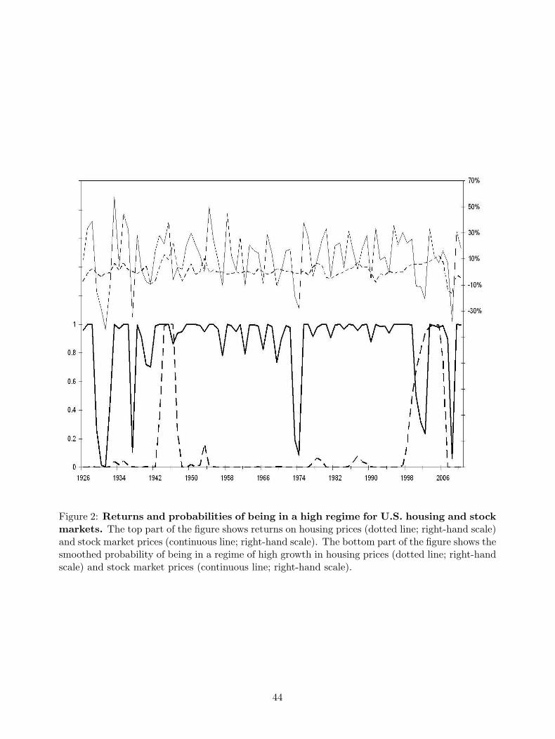
Figure 2: Returns and probabilities of being in a high regime for U.S. housing and stockmarkets. The top part of the figure shows returns on housing prices (dotted line; right-hand scale)and stock market prices (continuous line; right-hand scale). The bottom part of the figure shows thesmoothed probability of being in a regime of high growth in housing prices (dotted line; right-handscale) and stock market prices (continuous line; right-hand scale).

44

Figure 3: Probability of being in a high regime of house price returns and house pricereturns. U.S. census divisions. Probabilities of being in a high regime in continuous lines andvalues on the left-hand vertical axis. Housing returns in dotted lines and values according to theright-hand vertical axis. Graphs shown in the following order: Pacific (West) (Top), New England(Northeast), West South Central (South) and East North Central (Midwest) (Bottom).

45

Figure 4: Illustration. Hypothetical path of wealth-to-housing ratio and upper and lower boundsassociated with the two regimes. Changes in the expected growth of prices cause households tobuy or sell the house. When the ratio hits a bound, the benefits of re-sizing the house outweighsthe transaction costs.

46

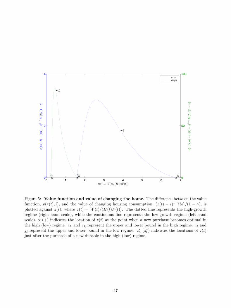
0 1 2 3 4 5 6 70

2

4

v(z(

t),l

)−(z

(t)−

ǫ)1−

γM

(l)/

(1−

γ)

xzl

xzl

+z∗l

0 1 2 3 4 5 6 70

50

100

z(t) = W(t)/(H(t)P(t))

v(z(

t),h

)−(z

(t)−

ǫ)1−

γM

(h)/

(1−

γ)

xzh

xzh

+z∗h

LowHigh

Figure 5: Value function and value of changing the home. The difference between the valuefunction, v(z(t), i), and the value of changing housing consumption, (z(t) − ε)1−γMi/(1 − γ), isplotted against z(t), where z(t) = W (t)/(H(t)P (t)). The dotted line represents the high-growthregime (right-hand scale), while the continuous line represents the low-growth regime (left-handscale). x (+) indicates the location of z(t) at the point when a new purchase becomes optimal inthe high (low) regime. zh and zh represent the upper and lower bound in the high regime. zl andzl represent the upper and lower bound in the low regime. z∗h (z∗l ) indicates the locations of z(t)just after the purchase of a new durable in the high (low) regime.

47

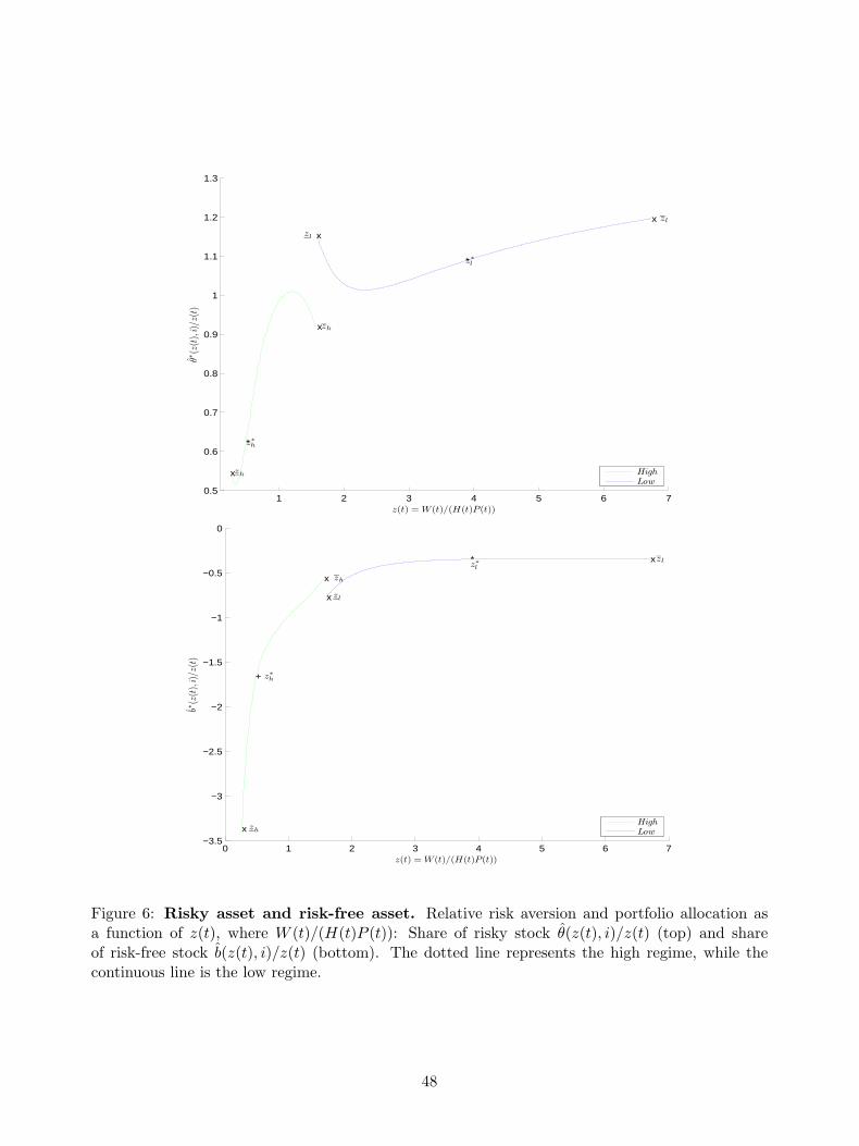
1 2 3 4 5 6 70.5

0.6

0.7

0.8

0.9

1

1.1

1.2

1.3

z(t) = W(t)/(H(t)P(t))

θ∗(z

(t),

i)/z(

t)

xzh

xzh

*z∗h

xzl

x zl

*z∗l

HighLow

0 1 2 3 4 5 6 7−3.5

−3

−2.5

−2

−1.5

−1

−0.5

0

z(t) = W(t)/(H(t)P(t))

b∗(z

(t),

i)/z(

t)

x zh

x zh

+ z∗h

x zl

xzl*z∗l

HighLow

Figure 6: Risky asset and risk-free asset. Relative risk aversion and portfolio allocation asa function of z(t), where W (t)/(H(t)P (t)): Share of risky stock θ(z(t), i)/z(t) (top) and shareof risk-free stock b(z(t), i)/z(t) (bottom). The dotted line represents the high regime, while thecontinuous line is the low regime.

48

Table 1: Parameter values for the house price and stock market process. Estimation of

the parameters of the house price process using a discrete Markov regime process. The growth of house prices in

each regime i is denoted by µi and its standard deviation is denoted by σ. In 2-regime processes, i can be either

i = l (low-growth regime) or i = h (high-growth regime). Column 1 shows the parameters for the U.S. house prices;

Columns 2 and 3 show the results for the stock markets. The likelihood test is used to test the null hypothesis that

house prices and the stock market follow a martingale against the alternative of a regime switching mechanism. All

parameters are reported on an annual basis. Source: Shiller (2005). Period: 1926− 2010.

House Prices Stock Markets Stock MarketsReal Nominal

(1) (2) (3)

µl -0.0049 -0.1625 -0.1990(0.0056) (0.0616) (0.0804)

µh 0.0925 0.1217 0.1272(0.0176) (0.0413) (0.0312)

σ 0.0447 0.1413 0.1473(0.0036) (0.0216) (0.0187)

λll 0.9658 0.3504 0.3515(0.0249) (0.1544) (0.1661)

λhl 0.2414 0.2453 0.1243(0.1494) (0.1589) (0.0985)

LR-test χ2 : µl = µh 14.326 2.729 5.115P-value 0.0119 0.9526 0.4739

49

Table 2: Parameter values for the house prices process - U.S. census divisions. Estimation

of the parameters of the house price process using a discrete Markov regime process. The growth of house prices in

each regime i is denoted by µi and its standard deviation is denoted by σP . In 2-regime processes, i can be either

i = l (low-growth regime) or i = h (high-growth regime). The unconditional probability of moving from regime i to

regime j is denoted by λij . Columns 1-9 show the parameters for the nine U.S. census divisions. The likelihood test

is used to test the null hypothesis that house prices follow a martingale against the alternative of a regime switching

mechanism. All parameters are reported on an annual basis. Source: OFHEO. Period: 1975− 2010.

Northeast Northeast Midwest MidwestNew England Middle East North West North

Atlantic Central Central(1) (2) (3) (4)

µl -0.0333 -0.0223 -0.0842 -0.1043(0.0086) (0.0095) (0.0081) (0.0164)

µh 0.0936 0.0790 0.0213 0.0179(0.0095) (0.0129) (0.0035) (0.0047)

σP 0.0322 0.0331 0.0179 0.0230(0.0021) (0.0027) (0.0011) (0.0018)

λll 0.9510 0.9627 0.8255 0.4992(0.0289) (0.0312) (0.0820) (0.1478)

λhl 0.0753 0.0666 0.0336 0.0654(0.0369) (0.0519) (0.0194) (0.0285)

LR-test χ2 : µl = µh 54.607 33.568 72.195 17.551P-value 0.0000 0.0000 0.0000 0.0029

South South South West WestSouth East South West South Mountain Pacific

Atlantic Central Central(5) (6) (7) (8) (9)

µl -0.0089 -0.1058 -0.0477 -0.0390 -0.0364(0.0059) (0.0249) (0.0126) (0.0088) (0.0084)

µh 0.0689 0.0102 0.0141 0.0451 0.0852(0.0160) (0.0049) (0.0059) (0.0078) (0.0082)

σP 0.0286 0.0221 0.0265 0.0313 0.0312(0.0018) (0.0016) (0.0017) (0.0020) (0.0019)

λll 0.9883 0.5007 0.9464 0.9650 0.9687(0.0120) (0.1794) (0.0546) (0.0297) (0.0219)

λhl 0.0806 0.0411 0.0152 0.0319 0.0425(0.0600) (0.0246) (0.0168) (0.0230) (0.0242)

LR-test χ2 : µl = µh 18.850 18.686 17.274 29.965 68.693P-value 0.0016 0.0017 0.0032 0.0000 0.0000

50

Table 3: Parameter used for benchmark calibration.

Variable Symbol ValueCurvature of the utility function γ 2House flow services 1− β 0.4Time preference ρ 0.025Risk free rate r 0.015House depreciation δ 0.02Transaction cost ε 0.05Risky asset drift αS 0.077Standard deviation risky asset σS 0.1655Correlation house price - risky asset ρPS 0.25

51

Table 4: Numerical results. Columns 1, 2 and 3 display the lower bound, the optimal return point and

the upper bound, respectively. The optimal return point represents the wealth-to-housing ratio immediately after

a housing purchase. Column 4 is the optimal housing-to-wealth ratio without transaction costs and Column 5 is

the corresponding ratio with transaction costs immediately after a housing purchase. Column 6 is the relative risk

aversion just after a housing purchase, and Column 7 is the average holding of the risky asset, estimated just after

a housing purchase. The first row in the table represents the benchmark case, described previously in this section.

Finally, we report the model results when we use the estimated house prices parameters for the nine U.S. census

divisions.

Regime (1) (2) (3) (4) (5) (6) (7)

i zi z∗i zi αh,i 1/z∗i RRA(z∗i )E

„θ∗(z∗,i)z∗

«E(τi)

U.S. aggregate High 0.249 0.491 1.587 2.980 2.035 2.595 0.730

(1930-2010) Low 1.575 3.870 6.739 0.340 0.258 2.071 1.098

U.S. census divisions

(1975-2010)

Northeast

New England High 0.254 0.470 1.171 3.111 2.124 2.740 0.703

Low 1.770 4.613 6.741 0.281 0.216 2.072 1.092

Middle Atlantic High 0.284 0.652 1.377 2.371 1.531 2.519 0.789

Low 1.809 3.831 6.743 0.288 0.260 2.106 1.090

Midwest

East North Central High 1.297 2.250 5.972 0.511 0.444 2.163 1.067

Low 2.849 7.207 12.443 0.160 0.138 2.022 1.138

West North Central High 1.520 2.459 6.874 0.406 0.370 2.140 1.080

Low 2.545 7.643 17.240 0.140 0.103 2.023 1.135

South

South Atlantic High 0.570 0.997 2.396 1.865 1.002 2.319 0.921

Low 2.066 3.601 6.748 0.307 0.277 2.125 1.086

East South Central High 1.675 3.799 6.178 0.405 0.263 2.052 1.100

Low 2.638 8.897 16.743 0.138 0.112 2.014 1.147

West South Central High 1.620 2.906 5.865 0.434 0.344 2.120 1.081

Low 2.686 5.590 9.137 0.204 0.178 2.030 1.127

West

Mountain High 0.890 1.425 2.992 0.979 0.701 2.289 0.965

Low 2.055 5.151 7.712 0.227 0.194 2.054 1.109

Pacific High 0.329 0.624 1.686 2.703 1.602 2.526 0.828

Low 1.863 4.676 7.508 0.259 0.213 2.071 1.103

52

Table 5: Descriptive statistics - PSID. Statistics for the main variables used in our analysis from PSID

data. The variables Move big and Move small correspond to the individuals who moved to a house having a higher

and lower value, respectively. Full sample refers to all the individuals in the sample, irrespective of their moving

situation. The ratio z = W/(P ·H) corresponds to the ratio of financial wealth net of debt over housing value without

considering human capital as part of the wealth. The ratio ez = (W + L)/(P · H) corresponds to the ratio of total

wealth with human capital L and net of debt over housing value. ∆ Family size shows the statistics of changes in

family size. ∆ Married is one if the individual gets married, zero otherwise. ∆ Employment is one if the individual

changes employment status, zero otherwise. Age corresponds to the age of the household head. Northeast, Midwest,

South and West are U.S. macro-region dummies.

Full sample Move big Move smallMean Std. err. Mean Std. err. Mean Std. err.

z = W/(PH) 1.388 1.645 1.322 1.780 1.257 1.640ez = (W + L)/(PH) 8.956 10.453 13.463 15.069 8.928 10.691Stock share (% financial wealth) Θ/W 0.102 0.225 0.124 0.248 0.107 0.200Stock (without retirement assets) share 0.056 0.146 0.065 0.181 0.059 0.155

(% financial wealth) bΘ/WStock (without retirement assets) share 0.189 0.339 0.176 0.321 0.192 0.344

(% liquid wealth) bΘ/cWSafe asset share -1.051 2.199 -1.644 2.679 -1.682 2.903(% financial wealth) B/WSafe asset (without debt) share 0.109 0.246 0.141 0.247 0.107 0.181

(% financial wealth) bB/WMove big 0.063 0.243 1.000 0.000 0.000 0.000Move small 0.023 0.149 0.000 0.000 1.000 0.000∆ Family -0.044 0.667 0.071 0.917 -0.235 1.150∆ Married 0.016 0.126 0.067 0.250 0.033 0.179∆ Employment 0.148 0.356 0.101 0.301 0.217 0.413Age 49.094 15.020 40.386 12.954 46.070 15.426Midwest 0.266 0.442 0.269 0.444 0.270 0.444South 0.409 0.492 0.389 0.488 0.425 0.495West 0.169 0.374 0.207 0.405 0.206 0.405Northeast 0.156 0.363 0.135 0.342 0.099 0.299

Num. Obs. 20189 1273 456

53

Table 6: Descriptive statistics - SIPP. Statistics for the main variables used in our analysis from SIPP

data. The variables Move big and Move small correspond to the individuals who moved to a house having a higher

and lower value, respectively. Full sample refers to all the individuals in the sample, irrespective of their moving

situation. The ratio z = W/(P ·H) corresponds to the ratio of financial wealth net of debt over housing value without

considering human capital as part of the wealth. The ratio ez = (W + L)/(P · H) corresponds to the ratio of total

wealth with human capital L and net of debt over housing value. ∆ Family size shows the statistics of changes in

family size. ∆ Married is one if the individual gets married, zero otherwise. ∆ Employment is one if the individual

changes employment status, zero otherwise. Age corresponds to the age of the household head. Northeast, Midwest,

South and West are U.S. macro-region dummies.

Full sample Move big Move smallMean Std. err. Mean Std. err. Mean Std. err.

z = W/(PH) 1.376 1.636 1.360 1.776 1.213 1.451ez = (W + L)/(PH) 5.944 7.153 9.019 8.932 5.099 5.894Stock share (% financial wealth) Θ/W 0.180 0.372 0.221 0.392 0.143 0.327Stock (without retirement assets) share 0.030 9.224 0.075 0.186 0.052 0.190

(% financial wealth) bΘ/WStock (without retirement assets) share 0.120 0.254 0.159 0.281 0.136 0.268

(% liquid wealth) bΘ/cWSafe asset share -0.779 2.187 -1.035 2.268 -0.929 2.181(% financial wealth) B/WSafe asset (without debt) share 0.052 6.887 0.085 0.208 0.072 0.157

(% financial wealth) bB/WMove big 0.017 0.129 1.000 0.000 0.000 0.000Move small 0.009 0.092 0.000 0.000 1.000 0.000∆ Family -0.015 0.508 0.077 0.728 -0.091 0.859∆ Married 0.011 0.106 0.011 0.105 0.048 0.215∆ Employment 0.069 0.253 0.097 0.297 0.127 0.334Age 52.987 15.741 43.802 12.979 49.436 15.263Midwest 0.272 0.445 0.279 0.449 0.249 0.433South 0.362 0.481 0.317 0.466 0.385 0.487West 0.185 0.389 0.260 0.439 0.226 0.419Northeast 0.180 0.384 0.144 0.351 0.139 0.347

Num. Obs. 105877 1797 911

54

Table 7: Movers. Percentage of households that moved over total households in the PSID and SIPP surveys

across all years. Column 1 captures the percentage of households that changed address. Column 2 captures the

percentage of households that moved to a new address in the same U.S. macro region. Column 3 captures the

percentage of households that moved to a new address in the same state. Column 4 shows the percentage of movers

that were not owners in the preceding period.

(a) PSID data

Status Move Same U.S. macro region Same U.S. state Not Owner at t− 1(1) (2) (3) (4)

Owner 15.43% 14.82% 14.19% 3.79%Renter 28.70% 27.03% 25.26% 25.31%Occupied 4.15% 3.87% 3.56% 3.63%

(b) SIPP data

Status Move Same U.S. macro region Same U.S. state Not Owner at t− 1(1) (2) (3) (4)

Owner 13.55% 12.74% 12.00% 5.47%Renter 35.16% 33.55% 32.17% 32.67%Occupied 3.49% 3.31% 3.09% 3.06%

Table 8: Test of Hypothesis 1 - PSID. Coefficients are estimated by using a standard OLS model and

ex-ante (i.e. before moving) values of zit as endogenous variable. mBIGit (mSMALLit) is a dummy variable equal to

one if the family is increasing (decreasing) its housing holdings (i.e. moving to a bigger (smaller) house). Standard

errors are reported in parentheses. ∗∗∗ denotes significance at the 1% level, ∗∗ at the 5% level, and ∗ at the 10% level.

The pooled regressions include year dummies. Source: PSID. Period: 1984− 2005.

All 1984 1989 1994 1999 2001 2003 2005constant (γ0) 2.166*** 1.949*** 0.831 1.022 2.006*** 2.056*** 1.361** 1.682***

(0.233) (0.542) (0.502) (0.524) (0.455) (0.444) (0.425) (0.404)mBIG (γ1) 2.456*** 4.166*** 4.206*** 1.667 4.305*** 1.922*** 2.016*** 1.732***

(0.235) (0.792) (0.830) (0.912) (0.631) (0.563) (0.489) (0.466)mSMALL (γ2) -0.438 0.487 0.066 -2.739 -1.118 0.027 0.687 -0.656

(0.378) (1.430) (1.529) (1.503) (0.961) (0.787) (0.872) (0.726)∆Family -0.352*** 0.128 -0.164 -0.226 -0.732*** -0.289 -0.365 -0.179

(0.086) (0.282) (0.296) (0.359) (0.208) (0.197) (0.191) (0.179)∆Married -0.041 0.696 -1.488 -3.944* 0.934 -0.866 0.665 1.372

(0.451) (1.509) (1.722) (1.751) (1.070) (1.052) (0.978) (0.928)∆Employment 0.135 -0.444 0.342 0.292 -0.254 0.398 0.494 0.789*

(0.161) (0.433) (0.433) (0.464) (0.449) (0.413) (0.422) (0.383)Agey<30 10.844*** 13.521*** 11.650*** 12.299*** 11.731*** 11.079*** 8.796*** 7.070***

(0.220) (0.576) (0.609) (0.688) (0.619) (0.580) (0.553) (0.491)Age30<y<40 8.706*** 9.064*** 9.656*** 10.327*** 9.006*** 8.875*** 7.447*** 6.645***

(0.168) (0.485) (0.453) (0.489) (0.436) (0.438) (0.423) (0.404)Age40<y<50 7.555*** 7.620*** 8.843*** 8.171*** 7.737*** 7.626*** 7.097*** 6.083***

(0.163) (0.547) (0.486) (0.482) (0.406) (0.400) (0.386) (0.365)Age50<y<60 4.355*** 5.097*** 3.769*** 5.202*** 4.426*** 4.747*** 3.786*** 3.481***

(0.174) (0.506) (0.511) (0.581) (0.473) (0.440) (0.409) (0.373)Midwest 1.424*** 0.127 2.673*** 2.540*** 1.582*** 0.842 1.626*** 1.037*

(0.178) (0.522) (0.510) (0.529) (0.468) (0.451) (0.432) (0.409)South 2.211*** 2.233*** 3.313*** 2.789*** 1.713*** 1.696*** 2.302*** 1.833***

(0.167) (0.483) (0.468) (0.500) (0.439) (0.424) (0.404) (0.381)West -1.198*** -1.637** -0.139 -0.351 -1.407** -1.755*** -1.192* -1.530***

(0.197) (0.584) (0.572) (0.607) (0.513) (0.495) (0.469) (0.438)R2 0.593 0.628 0.630 0.612 0.608 0.591 0.561 0.539Num. Obs. 20189 2507 2585 2457 3078 3191 3190 3181

55

Table 9: Test of Hypothesis 1 - SIPP. Coefficients are estimated by using a standard OLS model and

ex-ante (i.e. before moving) values of zit as endogenous variable. mBIGit (mSMALLit) is a dummy variable equal to

one if the family is increasing (decreasing) its housing holdings (i.e. moving to a bigger (smaller) house). Standard

errors are reported in parentheses. ∗∗∗ denotes significance at the 1% level, ∗∗ at the 5% level, and ∗ at the 10% level.

The pooled regressions include year dummies. Source: SIPP. Period: 1997-2005.

All 1997 1998 1999 2002 2003 2005constant (γ0) 3.471*** 2.103*** 2.214*** 2.308*** 2.111*** 1.875*** 1.702***

(0.530) (0.143) (0.141) (0.135) (0.132) (0.142) (0.108)mBIG (γ1) 1.677*** 1.847*** 1.988*** 2.424*** 1.415*** 1.512*** 1.049***

(0.153) (0.439) (0.396) (0.384) (0.379) (0.388) (0.286)mSMALL (γ2) -1.278*** -1.577** -1.603** -1.339* -1.483** -0.987 -0.818

(0.213) (0.570) (0.561) (0.543) (0.482) (0.579) (0.418)∆Family -0.371*** -0.572*** -0.369*** -0.383** -0.297** -0.478*** -0.211**

(0.040) (0.105) (0.102) (0.117) (0.095) (0.123) (0.070)∆Married -0.137 -0.447 0.567 -1.832** -0.333 0.124 0.371

(0.193) (0.500) (0.502) (0.607) (0.417) (0.613) (0.338)∆Employment -0.659*** -0.945*** -0.549* -0.907*** -0.712*** -0.592** -0.470***

(0.078) (0.264) (0.251) (0.240) (0.159) (0.188) (0.128)Agey<30 7.439*** 8.339*** 8.125*** 7.580*** 7.513*** 7.406*** 6.081***

(0.089) (0.237) (0.240) (0.231) (0.210) (0.232) (0.167)Age30<y<40 6.604*** 7.220*** 6.978*** 6.780*** 6.442*** 6.517*** 5.793***

(0.057) (0.150) (0.149) (0.144) (0.142) (0.153) (0.112)Age40<y<50 5.659*** 6.138*** 6.032*** 6.190*** 5.405*** 5.347*** 4.983***

(0.053) (0.143) (0.140) (0.133) (0.129) (0.139) (0.101)Age50<y<60 3.134*** 3.221*** 3.304*** 3.177*** 3.278*** 3.051*** 0.000

(0.057) (0.158) (0.152) (0.143) (0.137) (0.148) (.)Midwest 0.865*** 1.155*** 0.931*** 0.648*** 0.638*** 0.836*** 0.939***

(0.060) (0.158) (0.155) (0.148) (0.145) (0.157) (0.117)South 0.491*** 0.561*** 0.360* 0.382** 0.502*** 0.587*** 0.546***

(0.057) (0.150) (0.148) (0.142) (0.137) (0.147) (0.112)West -0.918*** -0.698*** -0.909*** -1.119*** -1.185*** -0.793*** -0.824***

(0.065) (0.174) (0.171) (0.162) (0.157) (0.168) (0.127)R2 0.516 0.506 0.518 0.543 0.538 0.494 0.508Num. Obs. 105216 18340 17095 16398 15572 15327 22484

56

Table 10: Test of Hypothesis 2a. Difference-in-differences regressions. Coefficients estimated using a

standard OLS model with ex-ante (i.e. before moving) values of zit. mBIGit (mSMALLit) is a dummy variable equal

to one if the family is increasing (decreasing) its housing holdings (i.e. moving to a bigger (smaller) house). HHMI

is an indicator capturing periods of persistent high appreciation in house prices at U.S. state level. Standard errors

are reported in parentheses. ∗∗∗ denotes significance at the 1% level, ∗∗ at the 5% level, and ∗ at the 10% level. The

regression includes year dummies. Source: PSID. Period: 1989− 2005.

All years

constant (γ0) 2.198***(0.254)

mBIG (γ1) 3.186***(0.319)

mSMALL (γ2) 0.404(0.336)

HHMI (γ3) -1.030***(0.203)

mBIG ×HHMI (γ4) -2.726***(0.604)

mSMALL ×HHMI (γ5) -0.893(0.980)

∆ Family -0.321***(0.095)

∆ Married 3.611***(0.496)

∆ Employment 0.705***(0.182)

Agey<30 6.735***(0.251)

Age30<y<40 5.374***(0.189)

Age40<y<50 4.623***(0.179)

Age50<y<60 2.429***(0.196)

Midwest 0.754***(0.209)

South 1.676***(0.196)

West -0.491*(0.219)

R2 0.416Num. Obs. 17280

57

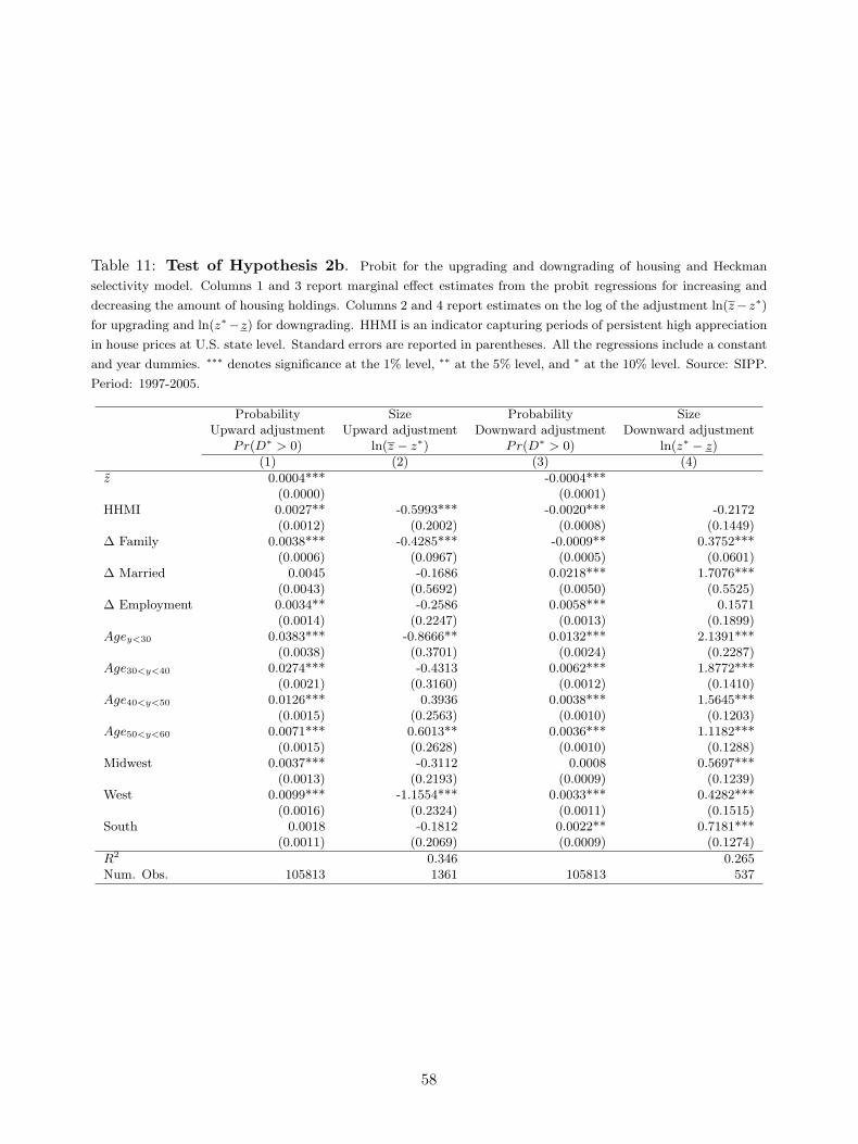
Table 11: Test of Hypothesis 2b. Probit for the upgrading and downgrading of housing and Heckman

selectivity model. Columns 1 and 3 report marginal effect estimates from the probit regressions for increasing and

decreasing the amount of housing holdings. Columns 2 and 4 report estimates on the log of the adjustment ln(z−z∗)for upgrading and ln(z∗−z) for downgrading. HHMI is an indicator capturing periods of persistent high appreciation

in house prices at U.S. state level. Standard errors are reported in parentheses. All the regressions include a constant

and year dummies. ∗∗∗ denotes significance at the 1% level, ∗∗ at the 5% level, and ∗ at the 10% level. Source: SIPP.

Period: 1997-2005.

Probability Size Probability SizeUpward adjustment Upward adjustment Downward adjustment Downward adjustment

Pr(D∗ > 0) ln(z − z∗) Pr(D∗ > 0) ln(z∗ − z)(1) (2) (3) (4)

z 0.0004*** -0.0004***(0.0000) (0.0001)

HHMI 0.0027** -0.5993*** -0.0020*** -0.2172(0.0012) (0.2002) (0.0008) (0.1449)

∆ Family 0.0038*** -0.4285*** -0.0009** 0.3752***(0.0006) (0.0967) (0.0005) (0.0601)

∆ Married 0.0045 -0.1686 0.0218*** 1.7076***(0.0043) (0.5692) (0.0050) (0.5525)

∆ Employment 0.0034** -0.2586 0.0058*** 0.1571(0.0014) (0.2247) (0.0013) (0.1899)

Agey<30 0.0383*** -0.8666** 0.0132*** 2.1391***(0.0038) (0.3701) (0.0024) (0.2287)

Age30<y<40 0.0274*** -0.4313 0.0062*** 1.8772***(0.0021) (0.3160) (0.0012) (0.1410)

Age40<y<50 0.0126*** 0.3936 0.0038*** 1.5645***(0.0015) (0.2563) (0.0010) (0.1203)

Age50<y<60 0.0071*** 0.6013** 0.0036*** 1.1182***(0.0015) (0.2628) (0.0010) (0.1288)

Midwest 0.0037*** -0.3112 0.0008 0.5697***(0.0013) (0.2193) (0.0009) (0.1239)

West 0.0099*** -1.1554*** 0.0033*** 0.4282***(0.0016) (0.2324) (0.0011) (0.1515)

South 0.0018 -0.1812 0.0022** 0.7181***(0.0011) (0.2069) (0.0009) (0.1274)

R2 0.346 0.265Num. Obs. 105813 1361 105813 537

58

Table 12: Test of Hypothesis 3 - PSID. Coefficients estimated using a standard OLS model and ex-ante

(i.e. before moving) values of the ratio of total risky stock holdings relative to financial wealth, Θit/Wit. mBIGit

(mSMALLit) is a dummy variable equal to one if the family is increasing (decreasing) its housing holdings (i.e. moving

to a bigger (smaller) house). Standard errors are reported in parentheses.∗∗∗

denotes significance at the 1% level,∗∗ at the 5% level, and ∗ at the 10% level. The pooled regressions include year dummies. Source: PSID. Period:

1984− 2005.All 1984 1989 1994 1999 2001 2003 2005

constant (γ0) 0.081*** 0.050*** 0.064*** 0.128*** 0.197*** 0.185*** 0.157*** 0.187***(0.006) (0.006) (0.007) (0.012) (0.013) (0.012) (0.019) (0.012)

mBIG (γ1) 0.030*** -0.008 0.037** 0.089*** 0.035* 0.035* 0.016 0.042**(0.007) (0.009) (0.012) (0.021) (0.018) (0.015) (0.022) (0.014)

mSMALL (γ2) 0.006 -0.007 0.017 -0.000 -0.008 0.031 0.037 -0.021(0.010) (0.017) (0.023) (0.035) (0.027) (0.022) (0.039) (0.021)

∆Family 0.003 0.001 0.010* 0.008 0.008 0.005 -0.003 0.000(0.002) (0.003) (0.004) (0.008) (0.006) (0.005) (0.009) (0.005)

∆Married -0.004 -0.010 -0.043 -0.056 0.005 -0.039 0.045 0.024(0.013) (0.018) (0.025) (0.040) (0.030) (0.029) (0.044) (0.027)

∆Employment -0.030*** -0.006 -0.011 -0.025* -0.034** -0.031** -0.055** -0.033**(0.004) (0.005) (0.006) (0.011) (0.013) (0.011) (0.019) (0.011)

Agey<30 -0.070*** -0.019** -0.027** -0.060*** -0.105*** -0.084*** -0.093*** -0.096***(0.006) (0.007) (0.009) (0.016) (0.017) (0.016) (0.025) (0.014)

Age30<y<40 -0.040*** -0.001 -0.018** -0.020 -0.049*** -0.058*** -0.053** -0.069***(0.005) (0.006) (0.007) (0.011) (0.012) (0.012) (0.019) (0.012)

Age40<y<50 -0.021*** -0.010 -0.011 0.001 -0.010 -0.030** -0.032 -0.045***(0.005) (0.007) (0.007) (0.011) (0.011) (0.011) (0.017) (0.011)

Age50<y<60 0.002 0.007 -0.006 0.007 0.003 0.004 -0.005 -0.004(0.005) (0.006) (0.008) (0.013) (0.013) (0.012) (0.018) (0.011)

Midwest -0.007 -0.003 0.016* -0.009 -0.015 -0.014 0.007 -0.024*(0.005) (0.006) (0.008) (0.012) (0.013) (0.012) (0.019) (0.012)

South -0.038*** -0.025*** -0.014* -0.040*** -0.067*** -0.051*** -0.018 -0.046***(0.005) (0.006) (0.007) (0.012) (0.012) (0.012) (0.018) (0.011)

West -0.010 -0.001 0.008 -0.007 -0.027 -0.006 0.012 -0.038**(0.005) (0.007) (0.008) (0.014) (0.014) (0.014) (0.021) (0.013)

R2 0.206 0.121 0.169 0.216 0.285 0.279 0.122 0.265Num. Obs. 20172 2491 2582 2459 3078 3191 3190 3181

59

Table 13: Test of Hypothesis 3 - SIPP. Coefficients estimated using a standard OLS model and ex-ante

(i.e. before moving) values of the ratio of total risky stock holdings relative to financial wealth, Θit/Wit. mBIGit

(mSMALLit) is a dummy variable equal to one if the family is increasing (decreasing) its housing holdings (i.e. moving

to a bigger (smaller) house). Standard errors are reported in parentheses.∗∗∗

denotes significance at the 1% level,∗∗ at the 5% level, and ∗ at the 10% level. The pooled regressions include year dummies. Source: SIPP. Period:

1997-2005.All 1997 1998 1999 2002 2003 2005

constant (γ0) 0.097*** 0.138*** 0.141*** 0.157*** 0.150*** 0.148*** 0.137***(0.027) (0.006) (0.006) (0.007) (0.008) (0.008) (0.006)

mBIG (γ1) 0.041*** 0.055** 0.052** 0.075*** 0.017 0.022 0.032*(0.008) (0.019) (0.018) (0.019) (0.022) (0.021) (0.016)

mSMALL (γ2) -0.032** -0.006 -0.017 -0.072** -0.033 -0.046 -0.022(0.011) (0.025) (0.026) (0.028) (0.028) (0.031) (0.024)

∆Family 0.005** 0.010* 0.024*** -0.000 -0.005 -0.004 0.002(0.002) (0.005) (0.005) (0.006) (0.006) (0.007) (0.004)

∆Married -0.009 -0.020 -0.018 -0.018 -0.024 -0.022 0.025(0.010) (0.022) (0.023) (0.031) (0.024) (0.033) (0.019)

∆Employment -0.016*** -0.022 -0.006 0.010 -0.030*** -0.020* -0.017*(0.004) (0.012) (0.011) (0.012) (0.009) (0.010) (0.007)

Agey<30 0.011* -0.002 -0.063*** -0.002 0.050*** 0.050*** 0.032***(0.005) (0.010) (0.011) (0.012) (0.012) (0.013) (0.009)

Age30<y<40 0.069*** 0.056*** 0.003 0.069*** 0.092*** 0.082*** 0.110***(0.003) (0.007) (0.007) (0.007) (0.008) (0.008) (0.006)

Age40<y<50 0.076*** 0.066*** 0.016* 0.074*** 0.102*** 0.088*** 0.105***(0.003) (0.006) (0.006) (0.007) (0.007) (0.008) (0.006)

Age50<y<60 0.075*** 0.061*** 0.030*** 0.070*** 0.106*** 0.087*** 0.092***(0.003) (0.007) (0.007) (0.007) (0.008) (0.008) (0.006)

Midwest 0.021*** 0.008 0.004 0.007 0.031*** 0.030*** 0.042***(0.003) (0.007) (0.007) (0.008) (0.008) (0.009) (0.007)

South -0.020*** -0.025*** -0.018** -0.034*** -0.022** -0.013 -0.008(0.003) (0.007) (0.007) (0.007) (0.008) (0.008) (0.006)

West -0.008* -0.002 0.004 -0.001 -0.017 -0.024** -0.009(0.003) (0.008) (0.008) (0.008) (0.009) (0.009) (0.007)

R2 0.261 0.232 0.179 0.273 0.284 0.263 0.314Num. Obs. 105154 18322 17086 16386 15564 15319 22477

60

Table 14: Test of Hypothesis 4 - IV Estimates. Columns (1) − (4) report OLS estimates of the

first stage effect of the house price index in the year of purchase, the house price index in the current year and the

interactions between these two indices and HHMI on the house value, home equity and the interactions between

the HHMI and the house value and home equity. Column (5) reports estimates of the effect of these variables and

HHMI on stock share of liquid wealth without including retirement assets in the stock holdings. Column (6) reports

estimates of the effect of these variables and HHMI on an indicator for holding stocks. All specifications include the

following set of controls: fixed effects of state residence, household head’s age, current year, and the year of purchase,

as well as 10-piece linear spline for liquid wealth, income, and number of children below 15 years. Standard errors are

reported in parentheses.∗∗∗

denotes significance at the 1% level, ∗∗ at the 5% level, and ∗ at the 10% level. Source:

SIPP. Period: 1997− 2005.House Value Home Equity House value Home equity Stockshare Stockholder

×HHMI ×HHMI liquid wealth(1) (2) (3) (4) (5) (6)

OFHEO state house price -109.703 -557.959*** -22.024 158.493***index of year purchase (1) (70.483) (63.026) (48.995) (41.758)

OFHEO state house price 2289.516*** 1837.614*** 956.072*** 420.418***index current year (2) (101.550) (90.805) (70.590) (60.163)

(1)×HHMI 64.756 -214.393** -79.232 -1968.013***(101.462) (90.727) (70.529) (60.111)

(2)×HHMI -209.274** -109.653 1508.566*** 1617.337***(102.699) (91.832) (71.389) (60.844)

HHMI 9531.251 23718.845*** 73798.365*** 111318.538*** 3.254 0.024(9986.046) (8929.453) (6941.584) (5916.235) (2.593) (0.047)

House value(×$100000) -2.165 -0.090*(2.594) (0.046)

Home equity(×$100000) 2.974 0.082*(2.767) (0.049)

House value 0.138 0.026×HHMI(×$100000) (1.475) (0.026)Home equity -2.690** -0.052**×HHMI(×$100000) (1.255) (0.022)R2 0.422 0.321 0.717 0.571 0.166 0.262Num. Obs. 43977 43977 43977 43977 43977 43977

61

Appendices

A.1 Derivation of the Model

A.1.1 Model Without Transaction Costs (ε = 0)

The value function is defined by

V (W (0), P (0), i) = supC,Θ,H

E

[∫ ∞0

e−ρtu(C,H)dt], i = 1, ..., n. (27)

The associated Hamilton-Jacobi-Bellman equation is the following in the regime i:

ρV (·, i) = supC,Θ,H

U(C,H) +DV (·, i) +∑i6=j

λij(V (·, j)− V (·, i))

, (28)

where

DV (·, i) = [r(W −HP ) + Θ(αS − r) + (µi − δ)HP − C]VW (·, i)

+ µiPtVP (·, i) +12

(Θ2σ2S + 2HPΘρPSσSσP +H2P 2σ2

P )VWW (·, i)

+12P 2σ2

P VPP (·, i) + (ΘPρPSσSσP +HP 2σ2P )VWP (·, i), i = 1, ..., n. (29)

We can use the homogeneity properties of the value function to reduce the problem with three state

variables (W,P, i) to one with two state variables, x = W/P and i, since

V (W,P, i) = P β(1−γ)V

(W

P, 1, i

)= P β(1−γ)v (x, i) , i = 1, ..., n. (30)

Let us introduce the scaled controls c = C/P and θ = Θ/P . Substituting and simplifying we obtain

ρiv(x, i) = supc,θ,H

U(c, H) +Dv(x, i) +∑i6=j

λij(v(x, j)− v(x, i))

, (31)

62

where

Dv(x, i) =((x−H)(r − µi + σ2P (1 + β(γ − 1))) + θ(αS − r − (1 + β(γ − 1))ρPSσSσP )− c)vx(x, i)

+12

((x−H)2σ2P − 2(x−H)θρPSσPσS + θ2σ2

S)vxx(x, i), i = 1, ..., n. (32)

Let

ρi = 0.5(−2ρ+ β(−1 + γ)(−2αi + (1 + β(γ − 1))σ2P ), i = 1, ..., n. (33)

We derive explicit expressions for both the value function and the optimal policies. We first guess

that the optimal controls are given by

c∗(x, i) = αc,ix, H∗(x, i) = αh,ix/P, θ∗(x, i) = αθ,ix (34)

and the value function for the no transaction costs problem is given by

v(x, i) = αv,ix1−γt

1− γ , (35)

where i = 1, ..., n. Then, we verify that the value function and the candidate control policies are

the optimal policies for the no transaction costs case.

A.1.2 Model With Transaction Costs (ε > 0)

The value function is defined by

V (W (0), P (0), H(0), i) = supC,Θ,H(τ),τ

E

[∫ τ

0e−ρtu(C,H)dt+ e−ρτV (W (τ), P (τ), H(τ), i)

], i = 1, ..., n.

(36)

We first solve the problem in the inaction region and then we try to characterize the upper and

lower bounds of the inaction region and the optimal return point between them. The associated

Hamilton-Jacobi-Bellman equation in the regime i is the following:37

ρV (·, l) = supC,Θ

U(C,H) +DV (·, i) +∑i6=j

λij(V (·, j)− V (·, i))

, (37)

37Thereafter, the notation V (·, i) refers to V (W,P,H, i).

63

where

DV (·, i) = [r(W −HP ) + Θ(αS − r) + (µi − δ)HP − C]VW (·, i)

+ µiPVP (·, i)− δHVH(·, i) +12

(Θ2σ2S + 2HPΘρPSσSσP +H2P 2σ2

P )VWW (·, i)

+12P 2σ2

PVPP (·, i) + (ΘPρPSσSσP +HP 2σ2P )VWP (·, i), i = 1, ..., n. (38)

The component λij(V (·, j)−V (·, i)) reflects the impact of the house price drift switch on the value

functions. This term is the product of the instantaneous probability of a regime shift and the

change in value function occurring after a regime switch. We can use the homogeneity properties

of the value function to reduce the problem with four state variables (W,P,H, i) to one with two

state variables, z = W/(PH) and i since

V (W,P,H, i) = H1−γP β(1−γ)V

(W

PH, 1, 1, i

)= H1−γP β(1−γ)v (z, i) , i = h, l. (39)

Let us introduce the scaled controls c = C/(PH) and θ = Θ/(PH). Substituting and simplifying,

we obtain

ρiv(z, i) = supc,θ

u(c) +Dv(z, i) +∑i6=j

λij(v(z, j)− v(z, i))

, (40)

where

u(c) =cβ(1−γ)

1− γ , (41)

Dv(z, i) =((z − 1)(r + δ − µi + σ2P (1 + β(γ − 1)))

+ θ(αS − r − (1 + β(γ − 1))ρPSσSσP )− c)vz(z, i)

+12

((z − 1)2σ2P − 2(z − 1)θρPSσPσS + θ2σ2

S)vzz(z, i), i = 1, ..., n. (42)

Let

ρi = 0.5(−2ρ− 2(γ − 1)(µi − δ + β(γ − 1)(1 + β(γ − 1))σ2P ), i = 1, ..., n. (43)

64

The first-order conditions are

c∗(z, i) =(vz(z, i)β

)1/(β(1−γ)−1)

, (44)

θ∗(z, i) = −(αS − r)vz(z, i)

σ2Svzz(z, i)

− (1− β(1− γ))ρPSσPvz(z, i)

σ2Svzz(z, i)

+ (z − 1)ρPSσPσS

, (45)

for i = 1, ..., n.

We need to identify the properties of the inaction region. It follows from (36) that

V (W (0), P (0), H(0), i) =

supC,Θ,H(τ),τ

E

[∫ τ

0e−ρτu(C,H(0)e−δt)dt+ e−ρτV (W (τ−)− εP (τ)H(τ−), P (τ), H(τ), i)

], i = 1, ..., n.

(46)

We get

P (0)β(1−γ)H(0)1−γv(z(0), i) =

supc,θ,H(τ),τ

E

[∫ τ

0e−ρτ

P (τ)β(1−γ)(cH(0)e−δt)1−γ

1− γ dt+ e−ρτP (τ)β(1−γ)H(τ)1−γv(z(τ), i)

], i = 1, ..., n.

(47)

Following Damgaard, Fuglsbjerg, and Munk (2003), let

e−ρτP (τ)β(1−γ)H(τ)1−γv(z(τ), i) =

e−ρτP (τ)β(1−γ)H(τ−)1−γ(H(τ−)H(τ)

)γ−1

v

(W (τ−)− εP (τ)H(τ−)

P (τ)H(τ), i

)=

e−ρτP (τ)β(1−γ)H(τ−)1−γ(H(τ−)H(τ)

)γ−1

v

(H(τ−)H(τ)

(W (τ−)

P (τ)H(τ−)− ε), i

)

and we can derive

e−ρτP (τ)β(1−γ)(H(0)e−δτ )1−γ (z(τ−)− ε)1−γ (H(τ−)

H(τ)(z(τ−)− ε

))γ−1

v

(H(τ−)H(τ)

(z(τ−)− ε

), i

)(48)

65

for i = 1, ..., n. Let us re-express our Bellman equation

P β(1−γ)v(z(0), i) =

supc,θ,τ

E

[∫ τ

0e−ρτ

P (τ)β(1−γ)c1−γ

1− γ dt+ e−ρτP (τ)β(1−γ)Mi(z(τ−)− ε)1−γ

1− γ

], (49)

where

Mi = supH(τ)≤He−δτ (z(τ−)ε)/ε

(1− γ)(H(τ−)H(τ)

(z(τ−)− ε

))γ−1

v

(H(τ−)H(τ)

(zτ− − ε) , i)

= (1− γ) supz≥ε

zγ−1v(z, i), i = 1, ..., n, (50)

and ρ = ρ+ δ(1− γ).

A.1.3 Algorithm for the Numerical Resolution

We modify the Grossman Laroque algorithm to solve our problem. The algorithm is a stepwise

numerical procedure to find the optimal values (Mi, zi, zi, z∗i ) for i = 1, ..., n:

1. Guess Mi = Mi,0 for i = 1, ..., n.

2. Solve the free bound problem as follows:

(i) Guess zi,0 for i = 1, ..., n;

(ii) Solve the ODEs Eq.(10) using as initial conditions the four equations defined by Eq.(15)

until the value-matching conditions are satisfied. We adopt a finite difference scheme to solve

the system of ODEs;

(iii) If the smooth pasting conditions specified by Eq.(16) are satisfied, then the candidate

value functions vMi,0(z, i) for i = 1, ..., n are found, otherwise repeat steps (i) and (ii).

3. Compute the implied M∗i,0 = (1−γ) supz zγ−1vMi,0(z, i) = (1−γ)z∗(γ−1)i v(z∗i , i) using Eq.(13).

If M∗i,0 = Mi,0 for each i = 1, ..., n, the problem is solved, otherwise go to step 1.

As a starting point, we use the solution to the problem of no transaction costs, ε = 0. That

solution consists of the optimal housing-to-wealth ratio αh,i, the optimal risky assets ratio αθ,i and

the optimal numeraire consumption ratio αc,i, for i = 1, ..., n. The first set of iterations uses a

66

fixed portfolio policy. For initial values of Mi and z∗i , we use Mi = αv,i and z∗i = 1/αh,i, where

i = 1, ..., n. However, there is little to guide the initial estimations about zi and zi, except to require

zi < z∗i and zi > z∗i . After the iterative procedure has converged, the solution is used to construct

an approximation to the policy function θ∗(z, i). Then, we adopt a value iteration procedure to

obtain (zi, zi,Mi, z∗i ) for i = 1, ..., n.

A.2 Sensitivity Analysis

Table 15 presents a sensitivity analysis of the model. It shows the sensitivity of three key variables

of the model (zi, z∗i ,zi) to four scenarios with deviations of four parameters from the benchmark

model. Moreover, Column (4) is the optimal housing-to-wealth ratio without transaction costs,

αh(i), and Column (5) is the corresponding ratio with transaction costs immediately after a housing

purchase, 1/z∗i . Column (6) is the relative risk aversion just after housing purchase, RRA(z∗i ), and

Column (7) is the average holding of the risky asset, estimated just after a housing purchase,

E(θ∗(z∗, i)/z∗i

)/E(τi).

[INSERT TABLE 15 HERE]

Scenario A illustrates how a change in the correlation between the house price and the risky

asset affects the optimal behavior. The optimal level z∗i decreases in both regimes, meaning that

housing consumption increases. In addition, the lower and upper bounds decrease as well. As

the correlation decreases, housing becomes more effective as a hedge to diversify away the stock

market risk, which leads to an increase in housing holdings. Furthermore, holding risky assets

becomes more attractive. In scenario B, we consider the sensitivity of our results to changes in the

transaction costs parameter ε. We find that a rise in transaction costs tends to widen the inaction

region and shift it to the right in both regimes. Increasing ε also decreases the optimal housing

holding. In scenario C, we vary the curvature coefficient γ from 2 to 3. As expected, the average

holding of risky assets falls from 0.730 to 0.536 in the high regime and from 1.098 to 0.730 in the

low regime; it is only substantially lower than the benchmark case in the high regime. Scenario

D shows that a decrease in house price volatility σP leads to a narrower inaction region and a

substantial increase in housing consumption. Moreover, housing is quite attractive for investment

67

purposes in the high regime, decreasing the average holding of risky assets from 0.730 to 0.629.

A.3 Estimation of the “Hot Housing Market Indicator” (HHMI)

This Appendix provides a detailed description of the ”Hot Housing Market Indicator” (HHMI). To

capture periods of persistent high appreciation in house prices at U.S. state level, we introduce this

as a binary variable that is calculated using the estimated smooth probabilities from the Markov-

switching model on real housing returns using the quarterly house price indexes for each state and

the U.S. aggregate. To go from these estimated probabilities to a binary variable, we assume that

the binary variable HHMIkt for the U.S. state k (i.e. k=California) at time t is equal to 1 when

the following two conditions hold:

1. the smooth probability of being in the regime associated with the highest expected real

housing return of the U.S. state k is higher than its historical average plus half of its historical

standard deviation in t, t− 1, t− 2 and t− 3 (four quarters in a row);

2. the real housing return of the state k is higher than the expected real housing return in the

high-growth regime of U.S. aggregate in t, t− 1, t− 2 and t− 3 (same four quarters of point

1).

The HHMI is based on these two conditions because they embed two specific pieces of information.

The first condition captures the likelihood that there has been a regime switch in the U.S. state k

based on a turning point probability. We define the turning point probability when the estimated

smooth probability reaches a 90% statistical level. The logic underlying the first condition is to

detect whether a housing market peak relative to its historical average in the state k has been

reached and it has lasted at least four quarters in a row.

Ideally, to infer the smooth probability of being in the regime with the highest expected real

housing return, the longest time series should be used. We estimate the Markov switching model

on the housing price indexes (HPI) published by the Office of Federal Housing Enterprise Oversight

(OFHEO) at U.S. state level. The index is a weighted repeat sales index that measures average

price changes in repeat sales or refinancing on the same properties and weights them. The price

information is obtained from repeat mortgage transactions on single-family properties whose mort-

68

gages have been purchased or securitized by Fannie Mae or Freddie Mac since the first quarter of

1975. While the housing price data has been criticized for its construction, to our knowledge it

is the best data available to the public at the state level. Subsequently, we work with the growth

rates of the housing price data, so issues related to bias in the level estimates are not relevant.

The house price indexes data are nominal. We deflate the data using core PCE inflation, which

measures inflation in the personal consumption expenditure basket less food and energy.

The house price indexes are available from 1975, but in our estimation we use only data be-

ginning in the first quarter of 1986 for some U.S. states. Figure 1 shows that HPI data at state

level are extremely noisy for a number of states before the mid-eighties. From the perspective of

the Markov switching model, the noise in the series is not necessarily a problem in terms of esti-

mation, but makes the regime classification uninformative when the time variation is very large, as

is the case for the HPI data. The noise abates considerably for most states after the mid-eighties.

Therefore, we estimate the Markov switching model on the subsample 1986(1)− 2010(4) for some

U.S. states using a volatility threshold criteria. If the house price index volatility of a U.S. state in

the subsample 1975(1) − 1985(4) is double the house price index volatility of the same U.S. state

in the subsample 1986(1) − 2010(4), we estimate the Markov switching model on the subsample

1986(1) − 2010(4) for that U.S. state. We have checked our results for robustness by (i) changing

the volatility threshold; and (ii) moving the start date to the first quarter of 1985, and have found

that the results are robust.

[INSERT FIGURE 7 HERE]

An important issue in estimating regime switching models is specifying the number of regimes.

This is often difficult to determine from data and as far as possible the choice should be based on

economic arguments (see Ang and Timmermann (2011)). It is not uncommon to simply fix the

number of regimes at some value, typically two or three, rather than basing the decision on econo-

metric tests. The reason is that tests for the number of regimes are typically difficult to implement

because they do not follow standard distributions. Because we aim to infer periods where house

prices grew markedly at U.S. state level and house price indexes have recently experienced a sharp

appreciation immediately followed by a sharp depreciation, we estimate a 3-regime specification.

In this case, the growth of house prices in each regime i is denoted by µi and i can be either i = l

69

(low-growth regime), i = m (medium-growth regime) or i = h (high-growth regime).

Table 16 reports the parameter estimates for the U.S. states. Overall, our analysis suggests that

U.S. states differ markedly in the level of and spread between the high and low-phase growth rates.

Using a likelihood ratio test, we test the null hypothesis that house prices follow a martingale against

the alternative of a regime switching mechanism. Then, we provide the Regime Classification

Measure (RCM) which captures the quality of a model’s regime qualification performance developed

by Ang and Bekaert (2002). They argue that a good regime-switching model should be able to

classify regimes sharply. This is the case when the smoothed (ex-post) regime probabilities pi are

close to either one or zero. Inferior models, however, will exhibit pi values closer to 1/k, where k is

the number of regimes. A perfect model will be associated with a RCM close to zero, while a model

that cannot distinguish between regimes at all will produce a RCM close to 100. Ang and Bekaert’s

(2002) generalization of this formula to the multiple state case has many undesirable features.38

We therefore adopt the measure adapted by Baele (2005):

RCM = 100×(

1− k

k − 11T

T∑t=1

k∑i=1

(pi,t −

1κ

)2)

(51)

lies between 0 and 100, where the latter means that the model cannot distinguish between the

regimes. Therefore, lower RCM values denote better regime classification. Overall, a 3-regime

specification allows a clear regime-classification of the HPI data.

[INSERT TABLE 16 HERE]

According to the second condition of HHMI, the real housing return of the state k has to be

higher than the expected real housing return in the high-growth regime of U.S. aggregate for four

quarters in a row. A natural candidate of the expected real housing return at U.S. aggregate level

is the expected growth rate in the high regime we estimated using the long Case-Shiller HPI time

series dating back to 1925. The estimated mean of the real annual growth rate is 9.25% during

the high-growth regimes. Although, OFHEO’s HPI data and the house price indexes produced by

Case-Shiller are constructed using the same basic methodology, important differences between the

indexes remain. The two models use different data sources and implement the mechanics of the basic38More specifically, their measure produces small RCMs as soon as one regime has a very low probability, even if

the model cannot distinguish between the other regimes.

70

algorithm in distinct ways.39 Therefore, it is not appropriate to use the estimated mean of 9.25%

as a threshold. The OFHEO’s HPI is a good estimate of the typical price appreciation of single-

family houses, whereas the Case-Shiller index is a good estimate of the capital appreciation that

would result from owning a representative sample of U.S. homes. The HPI tends to underrepresent

high-priced homes; it also tends to underrepresent low-priced homes. The reason is that Fannie and

Freddie only purchase conventional loans, which typically exclude smaller-sized mortgages that are

insured by the Veterans Administration and the Federal Housing Administration.40 These and the

previous exclusions imply that the HPI is best interpreted as measuring aggregate price appreciation

for a broad middle segment of the U.S. stock of single-family homes. As a consequence of its value

weighting, the Case-Shiller index growth rate systematically differs from the HPI growth rate. For

example, Case-Shiller index growth consistently exceeds HPI growth, starting in 1998. Over the

subsequent six years, it does so by as much as four percentage points in some quarters. Then, HPI

growth consistently exceeds Case-Shiller index growth starting in the first quarter of 2006 when

house prices started to markedly depreciate. Alternatively, we can obtain our threshold using the

regime classification inferred by our 2-regime model using the long Case-Shiller HPI time series.

Based on the smooth probabilities, only the period 2000 − 2006 is associated with a high growth

phase over the period 1975− 2010. We calculate a mean annual real growth rate of 6.87% during

high regimes using the HPI at U.S. aggregate level.41 Accordingly, we use this as our threshold.

39 Both use the repeat-valuations framework initially proposed in the 1960s40Also excluded from the HPI are condominiums, co-ops, and other multifamily homes.41We have also checked our results for a 3-regime specification on the Case-Shiller HPI for robustness. The period

2000 − 2006 is still associated with a high-growth phase. Specifically, we obtain (standard errors in parenthesis)µl = −0.1484 (0.0334), µm = −0.0004 (0.0047), µh = 0.0944 (0.0145), σP = 0.0375 (0.0030), λll = 0.4206 (0.3210),λmm = 0.9674 (0.0233), λlh = 0.1019 (0.1008) and λmh = 0.1167 (0.1244). The low regime is associated with sharphouse price depreciation, starting in 2006.

71

Figures and Tables of the Appendix

1975 1980 1985 1990 1995 2000 2005 2010

−0.25

−0.2

−0.15

−0.1

−0.05

0

0.05

0.1

0.15

0.2

0.25

Figure 7: Housing returns - U.S. states. This figure shows the growth rates in OFHEO houseprice indexes for the U.S. states for the period 1975− 2010. The vertical line marks 1986−Q1.

72

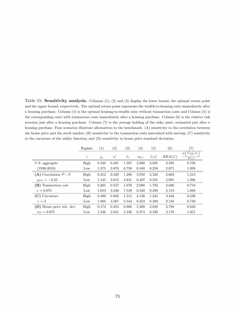
Table 15: Sensitivity analysis. Columns (1), (2) and (3) display the lower bound, the optimal return point

and the upper bound, respectively. The optimal return point represents the wealth-to-housing ratio immediately after

a housing purchase. Column (4) is the optimal housing-to-wealth ratio without transaction costs and Column (5) is

the corresponding ratio with transaction costs immediately after a housing purchase. Column (6) is the relative risk

aversion just after a housing purchase. Column (7) is the average holding of the risky asset, estimated just after a

housing purchase. Four scenarios illustrate alternatives to the benchmark: (A) sensitivity to the correlation between

the house price and the stock market; (B) sensitivity to the transaction costs associated with moving; (C) sensitivity

to the curvature of the utility function; and (D) sensitivity to house price standard deviation.

Regime (1) (2) (3) (4) (5) (6) (7)

i zi z∗i zi αh,i 1/z∗i RRA(z∗i )E

„θ∗(z∗,i)z∗

«E(τi)

U.S. aggregate High 0.249 0.491 1.587 2.980 2.035 2.595 0.730

(1930-2010) Low 1.575 3.870 6.739 0.340 0.258 2.071 1.098

(A) Correlation P - S High 0.212 0.429 1.286 3.950 2.328 2.663 1.213

ρPS = −0.25 Low 1.145 3.012 4.841 0.497 0.331 2.091 1.096

(B) Transaction cost High 0.265 0.557 1.678 2.980 1.792 2.686 0.718

ε = 0.075 Low 1.653 3.346 7.549 0.340 0.298 2.153 1.080

(C) Curvature High 0.490 0.802 1.515 2.138 1.245 3.448 0.536

γ = 3 Low 1.866 3.567 5.544 0.324 0.280 3.156 0.730

(D) House price std. dev. High 0.174 0.353 0.866 5.208 2.828 2.788 0.629

σP = 0.075 Low 1.546 3.021 5.240 0.374 0.330 2.170 1.051

73

Tab

le16:

Par

amet

erva

lues

for

the

hou

sep

rice

sp

roce

ss-

U.S

.st

ates

.E

stim

ati

on

of

the

para

met

ers

of

the

hou

sep

rice

pro

cess

esu

sin

ga

dis

cret

eM

ark

ov

regim

e-sw

itch

ing

mod

el.

Th

egro

wth

of

hou

sep

rice

sin

each

regim

ei

is

den

ote

dbyµi

an

dit

sst

an

dard

dev

iati

on

isd

enote

dbyσP

.In

3-r

egim

ep

roce

sses

,i

can

be

eith

eri

=l

(low

-gro

wth

regim

e),

i=m

(med

ium

-gro

wth

regim

e)ori

=h

(hig

h-g

row

thre

gim

e).

Th

eu

nco

nd

itio

nal

pro

bab

ilit

yof

movin

gfr

om

regim

ei

to

regim

ej

isd

enote

dbyλij

.T

he

likel

ihood

test

isu

sed

tote

stth

enu

llhyp

oth

esis

that

hou

sep

rice

sfo

llow

am

art

ingale

again

stth

ealt

ern

ati

ve

of

are

gim

esw

itch

ing

mec

han

ism

.R

CM

refe

rsto

the

An

g-B

ekaer

t(2

000)

regim

ecl

ass

ifica

tion

mea

sure

100ד 1−

kk−

11 T

P T t=1

P k i=1

` p i,t−

1 κ

´ 2” ,w

her

epi,t

isth

esm

ooth

edre

gim

ep

rob

ab

ilit

yan

dk

isth

enu

mb

erof

regim

es.

Low

er

RC

Mvalu

esd

enote

bet

ter

regim

ecl

ass

ifica

tion

.A

llp

ara

met

ers

are

rep

ort

edin

qu

art

erly

basi

s.S

ou

rce:

OF

HE

O.

Per

iod

:*

1975−

2010

-**

1986−

2010.

µl

µm

µh

σP

λll

λml

λlm

λmm

λlh

λmh

LR

-tes

tχ

2R

CM

North

east

New

En

gla

nd

Main

e**

−0.0

222

0.0

052

0.0

222

0.0

095

0.4

254

0.2

662

0.7

075

0.0

625

57.9

27

17.9

99

(0.0

030)

(0.0

019)

(0.0

024)

(0.0

008)

(0.1

593)

(0.0

884)

(0.0

925)

(0.0

440)

(0.0

000)

New

Ham

psh

ire*

*−

0.0

376−

0.0

049

0.0

218

0.0

122

0.6

007

0.0

845

0.8

927

0.0

521

70.3

50

12.3

55

(0.0

060)

(0.0

023)

(0.0

022)

(0.0

010)

(0.1

872)

(0.0

542)

(0.0

589)

(0.0

360)

(0.0

000)

Ver

mont*

*−

0.0

055

0.0

100

0.0

260

0.0

117

0.9

710

0.0

788

0.8

761

0.1

177

45.0

14

20.0

66

(0.0

019)

(0.0

028)

(0.0

033)

(0.0

009)

(0.0

303)

(0.0

566)

(0.0

734)

(0.0

840)

(0.0

000)

Mass

ach

use

tts*

−0.0

152

0.0

083

0.0

315

0.0

137

0.8

599

0.1

237

0.8

342

0.0

592

84.8

29

25.1

71

(0.0

029)

(0.0

043)

(0.0

037)

(0.0

010)

(0.0

774)

(0.0

720)

(0.0

787)

(0.0

447)

(0.0

000)

Rh

od

eIs

lan

d*

−0.0

731−

0.0

069

0.0

374

0.0

213

0.0

003

0.0

257

0.9

425

0.1

448

48.5

79

11.9

83

(0.0

256)

(0.0

032)

(0.0

049)

(0.0

018)

(1.4

120)

(0.0

349)

(0.0

398)

(0.0

64)

(0.0

000)

Con

nec

ticu

t*−

0.0

126

0.0

170

0.0

4399

0.0

174

0.9

039

0.0

460

0.0

324

0.9

379

0.3

658

0.0

021

46.3

73

17.6

66

(0.0

093)

(0.0

092)

(0.0

150)

(0.0

054)

(0.1

432)

(0.1

616)

(0.1

448)

(0.1

461)

(0.6

637)

(1.5

52)

(0.0

000)

North

east

Mid

dle

Atl

anti

c

New

York

*−

0.0

761−

0.0

048

0.0

260

0.0

186

0.0

115

0.9

750

0.0

179

0.0

391

54.1

31

8.2

20

(0.0

134)

(0.0

022)

(0.0

029)

(0.0

011)

(0.0

118)

(0.0

175)

(0.0

181)

(0.0

274)

(0.0

000)

New

Jer

sey*

−0.0

434−

0.0

029

0.0

277

0.0

140

0.2

882

0.0

505

0.9

118

0.0

1637

0.0

525

73.7

13

12.2

21

74

Tab

le16

–conti

nu

ed

from

previo

us

page

µl

µm

µh

σP

λll

λml

λlm

λmm

λlh

λmh

LR

-tes

tχ

2R

CM

(0.0

187)

(0.0

036)

(0.0

024)

(0.0

015)

(0.2

862)

(0.0

693)

(0.0

751)

(0.0

246)

(0.0

373)

(0.0

000)

Pen

nsy

lvan

ia*

−0.0

325

0.0

002

0.0

198

0.0

113

0.4

539

0.0

131

0.9

551

0.1

600

0.0

890

55.5

92

15.1

25

(0.0

030)

(0.0

019)

(0.0

025)

(0.0

008)

(0.1

294)

(0.0

162)

(0.0

274)

(0.0

642)

(0.0

49)

(0.0

000)

Sou

th

East

Sou

thC

entr

al

Ken

tuck

y**

−0.0

100

0.0

044

0.0

209

0.0

064

0.6

374

0.2

257

0.0

368

0.4

557

0.0

591

26.7

76

12.9

19

(0.0

054)

(0.0

009)

(0.0

052)

(0.0

006)

(0.2

864)

0.4

004

(0.0

300)

(0.3

483)

(0.3

578)

(0.0

016)

Ten

nes

see*

*−

0.0

119

0.0

050

0.0

229

0.0

073

0.8

185

0.1

165

0.0

344

0.2

408

0.2

161

34.5

71

8.7

66

(0.0

026)

(0.0

009)

(0.0

048)

(0.0

006)

(0.1

190)

0.1

021

(0.0

248)

(0.2

351)

(0.2

283)

(0.0

001)

Mis

siss

ipp

i**

−0.0

195

0.0

047

0.0

088

0.0

087

0.4

361

0.0

022

0.0

007

0.9

801

0.6

258

0.0

563

35.5

94

11.9

73

(0.0

034)

(0.0

013)

(0.0

034)

(0.0

008)

(0.1

933)

(0.3

675)

(0.0

827)

(0.0

250)

(0.3

620)

(0.4

156)

(0.0

001)

Ala

bam

a**

−0.0

111

0.0

046

0.0

165

0.0

079

0.7

677

0.0

572

0.0

185

0.4

764

0.0

006

25.6

06

7.9

79

(0.0

022)

(0.0

010)

(0.0

039)

(0.0

006)

(0.1

107)

(0.0

582)

(0.0

227)

(0.1

947)

(0.2

148)

(0.0

025)

Sou

th

Sou

thA

tlanti

c

Del

aw

are

**

−0.0

084

0.0

100

0.0

243

0.0

099

0.9

676

0.0

701

0.8

946

0.1

078

64.4

29

15.8

91

(0.0

017)

(0.0

022)

(0.0

034)

(0.0

008)

(0.0

339)

(0.0

505)

(0.0

615)

(0.0

784)

(0.0

000)

Mary

lan

d*

−0.0

513−

0.0

006

0. 0

268

0.0

1374

0.4

128

0.3

000

0.0

279

0.9

496

0.0

216

0.0

941

62.8

01

10.0

50

(0.0

071)

(0.0

016)

(0.0

029)

(0.0

009)

(0.2

104)

(0.2

457)

(0.0

200)

(0.0

252)

(0.0

308)

(0.0

527)

(0.0

000)

Dis

tric

tof

Colu

mb

ia**

−0.0

327

0.0

005

0.0

298

0.0

131

0.2

827

0.1

337

0.8

411

0.0

506

60.9

73

13.1

45

(0.0

072)

(0.0

025)

(0.0

025)

(0.0

011)

(0.2

090)

(0.0

670)

(0.0

715)

(0.0

354)

(0.0

000)

Vir

gin

ia*

−0.0

873−

0.0

047

0. 0

168

0.0

130

0.0

117

0.9

731

0.0

405

68.5

79

9.4

91

(0.0

131)

(0.0

016)

(0.0

020)

(0.0

007)

(0.0

117)

(0.0

191)

(0.0

289)

(0.0

000)

Wes

tV

irgin

ia**

−0.0

216

0.0

066

0.0

863

0.0

097

0.2

661

0.1

535

0.5

000

36.9

07

9.7

68

(0.0

034)

(0.0

012)

(0.0

097)

(0.0

008)

(0.1

416)

(0.0

517)

(0.3

536)

(0.0

000)

Nort

hC

aro

lin

a*

−0.0

230

0.0

040

0.0

096

0.0

088

0.2

579

0.0

007

0.0

123

0.9

876

0.3

971

0.0

352

50.0

36

9.9

33

(0.0

076)

(0.0

014)

(0.0

036)

(0.0

008)

(0.3

267)

(0.4

336)

(0.0

130)

(0.0

133)

(0.2

161)

(0.0

722)

(0.0

000)

Sou

thC

aro

lin

a*

−0.0

251

0.0

041

0.0

205

0.0

102

0.3

828

0.0

243

0.0

258

0.5

697

0.0

984

58.3

83

3.4

44

75

Tab

le16

–conti

nu

ed

from

previo

us

page

µl

µm

µh

σP

λll

λml

λlm

λmm

λlh

λmh

LR

-tes

tχ

2R

CM

(0.0

030)

(0.0

011)

(0.0

027)

(0.0

006)

(0.1

249)

0.0

826

(0.0

191)

(0.1

139)

(0.0

809)

(0.0

000)

Geo

rgia

*−

0.0

201

0. 0

043

0.0

162

0.0

098

0.5

086

0.0

066

0.0

304

0.6

338

0.1

153

45.3

67

12.1

36

(0.0

025)

(0.0

022)

(0.0

034)

(0.0

014)

(0.1

201)

(0.1

164)

(0.0

489)

(0.1

476)

(0.1

248)

(0.0

000)

Flo

rid

a*

−0.0

457

0. 0

027

0.0

541

0.0

186

0.7

524

0.0

641

0.0

105

0.9

797

0.2

194

0.1

504

68.8

23

5.4

37

(0.0

053)

(0.0

018)

(0.0

064)

(0.0

011)

(0.1

152)

(0.0

733)

(0.0

106)

(0.0

143)

(0.1

197)

(0.1

028)

(0.0

000)

Sou

th

West

Sou

thC

entr

al

Okla

hom

a*

−0.0

331

0.0

013

0.0

304

0.0

097

0.4

078

0.3

504

0.0

600

0.9

110

0.2

996

0.2

598

52.2

86

7.9

07

(0.0

044)

(0.0

012)

(0.0

029)

(0.0

008)

(0.1

387)

(0.1

459)

(0.0

278)

(0.0

383)

(0.1

821)

(0.2

148)

(0.0

000)

Ark

an

sas*

*−

0.0

187−

0.0

048

0.0

058

0.0

078

0.2

870

0.4

577

0.2

958

0.7

041

0.0

583

24.7

33

17.3

41

(0.0

034)

(0.0

042)

(0.0

010)

(0.0

007)

(0.1

875)

(0.2

577)

(0.3

208)

(0.2

576)

(0.0

363)

(0.0

036)

Tex

as*

−0.0

281

0.0

014

0.0

261

0.0

091

0.4

099

0.3

379

0.0

573

0.9

152

0.2

640

0.2

358

44.0

45

10.1

64

(0.0

035)

(0.0

010)

(0.0

026)

(0.0

007)

(0.1

416)

(0.1

517)

(0.0

319)

(0.0

348)

0.1

255

(0.1

337)

(0.0

000)

Lou

isia

na*

−0.0

117

0.0

068

0.0

313

0.0

121

0.8

502

0.0

207

0.0

174

0.6

076

0.0

001

41.2

59

8.9

93

(0.0

018)

(0.0

016)

(0.0

043)

(0.0

008)

(0.0

548)

(0.0

214)

(0.0

175)

(0.1

555)

(0.0

451)

(0.0

000)

Mid

west

West

North

Centr

al

Nort

hD

akota

**

−0.0

173

0.0

049

0.0

239

0.0

108

0.6

555

0.0

643

0.9

712

30.7

21

3.8

81

(0.0

034)

(0.0

012)

(0.0

069)

(0.0

008)

(0.1

542)

(0.0

632)

(0.2

735)

(0.0

000)

Sou

thD

akota

**

−0.0

166

0.0

058

0.0

201

0.0

079

0.4

892

0.0

623

0.0

358

0.9

607

0.5

382

0.1

266

36.7

81

8.4

94

(0.0

020)

(0.0

011)

(0.0

026)

(0.0

006)

(0.1

257)

(0.0

714)

(0.0

397)

(0.0

275)

(0.1

432)

(0.1

007)

(0.0

001)

Min

nes

ota

*−

0.0

390−

0.0

008

0. 0

159

0.0

110

0.3

599

0.3

017

0.0

631

0.9

145

0.0

428

0.0

716

56.7

94

18.8

27

(0.0

069)

(0.0

019)

(0.0

019)

(0.0

012)

(0.1

586)

(0.1

947)

(0.0

668)

(0.0

734)

(0.0

353)

(0.0

525)

(0.0

000)

Neb

rask

a**

−0.0

104

0.0

039

0.0

233

0.0

064

0.6

969

0.2

496

0.0

605

0.9

266

0.5

179

0.0

049

26.4

07

14.1

45

(0.0

024)

(0.0

011)

(0.0

037)

(0.0

006)

(0.1

377)

(0.1

395)

(0.0

407)

(0.0

435)

(0.5

623)

(0.6

278)

(0.0

044)

Iow

a**

−0.0

275

0.0

030

0.0

249

0.0

076

0.3

525

0.0

214

0.9

400

29.2

15

1.0

568

(0.0

049)

(0.0

008)

(0.0

073)

(0.0

005)

(0.2

819)

(0.0

150)

(0.4

203)

(0.0

001)

Kan

sas*

*−

0.0

093

0.0

047

0.0

240

0.0

065

0.8

873

0.0

745

0.0

184

0.9

695

0.6

103

0.0

285

43.9

07

7.7

04

76

Tab

le16

–conti

nu

ed

from

previo

us

page

µl

µm

µh

σP

λll

λml

λlm

λmm

λlh

λmh

LR

-tes

tχ

2R

CM

(0.0

016)

(0.0

008)

(0.0

044)

(0.0

005)

(0.0

652)

(0.0

550)

(0.0

201)

(0.0

228)

(0.4

215)

(0.3

554)

(0.0

000)

Mis

sou

ri**

−0.0

108

0. 0

056

0.0

218

0.0

070

0.8

596

0.0

703

0.0

305

0.9

694

0.5

967

43.5

63

8.9

70

(0.0

020)

(0.0

009)

(0.0

076)

(0.0

006)

(0.0

860)

(0.0

728)

(0.0

284)

(0.0

276)

(0.5

321)

(0.0

000)

Mid

west

East

North

Centr

al

Mic

hig

an*

−0.0

345

0.0

062

0.0

966

0.0

123

0.6

646

0.2

910

0.0

624

77.1

62

5.6

45

(0.0

044)

(0.0

012)

(0.0

123)

(0.0

008)

(0.1

382)

(0.1

320)

(0.0

248)

(0.0

000)

Wis

con

sin

**

−0.0

146

0.0

048

0.0

247

0.0

073

0.8

164

0.0

823

0.9

445

0.2

709

0.4

897

32.9

08

5.4

26

(0.0

023)

(0.0

008)

(0.0

034)

(0.0

006)

(0.1

183)

(0.0

954)

(0.0

291)

(0.1

726)

(0.2

036)

(0.0

001)

Illin

ois

*−

0.0

356

0.0

007

0.0

084

0.0

099

0.3

408

0.6

093

0.5

479

0.3

626

0.0

213

86.6

01

7.9

66

(0.0

032)

(0.0

034)

(0.0

009)

(0.0

006)

(0.1

421)

(0.1

934)

(0.1

920)

(0.1

938)

(0.0

163)

(0.0

000)

Ind

ian

a**

−0.0

215

0.0

022

0.0

219

0.0

063

0.3

473

0.4

441

0.0

303

0.2

169

0.2

087

38.4

97

3.1

04

(0.0

038)

(0.0

008)

(0.0

033)

(0.0

007)

(0.2

497)

(0.3

199)

(0.0

350)

(0.1

962)

(0.1

929)

(0.0

000)

Oh

io*

−0.0

292

0.0

002

0.0

042

0.0

089

0.4

746

0.3

532

0.4

509

0.5

927

0.0

744

0.0

540

60.7

48

15.4

68

(0.0

035)

(0.0

033)

(0.0

010)

(0.0

005)

(0.1

708)

(0.2

671)

(0.2

501)

(0.3

826)

(0.1

430)

(0.1

284)

(0.0

000)

West

Pacifi

c

Haw

aii**

−0.0

108

0.0

128

0.0

451

0.0

141

0.9

744

0.0

727

0.8

371

0.1

369

82.2

39

13.8

50

(0.0

021)

(0.0

032)

(0.0

039)

(0.0

011)

(0.0

251)

(0.0

507)

(0.0

804)

(0.0

982)

(0.0

000)

Ala

ska*

−0.1

663

0.0

023

0.1

183

0.0

290

0.7

589

0.0

286

0.9

514

0.8

011

62.9

56

2.0

81

(0.0

167)

(0.0

026)

(0.0

219)

(0.0

019)

(0.2

149)

(0.0

149)

(0.0

201)

(0.2

657)

(0.0

000)

Wash

ingto

n*

−0.0

390

0.0

034

0.0

367

0.0

106

0.4

117

0.3

867

0.0

598

0.9

101

0.2

059

86.7

46

5.2

75

(0.0

043)

(0.0

011)

(0.0

023)

(0.0

006)

(0.1

621)

(0.1

647)

(0.0

244)

(0.0

294)

(0.0

839)

(0.0

000)

Ore

gon

**

−0.0

206

0.0

089

0.0

296

0.0

094

0.8

070

0.0

452

0.9

213

0.1

869

56.8

84

12.6

14

(0.0

040)

(0.0

015)

(0.0

039)

(0.0

008)

(0.1

328)

(0.0

262)

(0.0

387)

(0.1

213)

(0.0

000)

Califo

rnia

*−

0.0

750−

0.0

075

0.0

267

0.0

141

0.7

292

0.0

150

0.9

537

0.0

4310

126.9

45.8

48

(0.0

086)

(0.0

019)

(0.0

018)

(0.0

008)

(0.2

330)

(0.0

149)

(0.0

261)

(0.0

244)

(0.0

000)

West

77

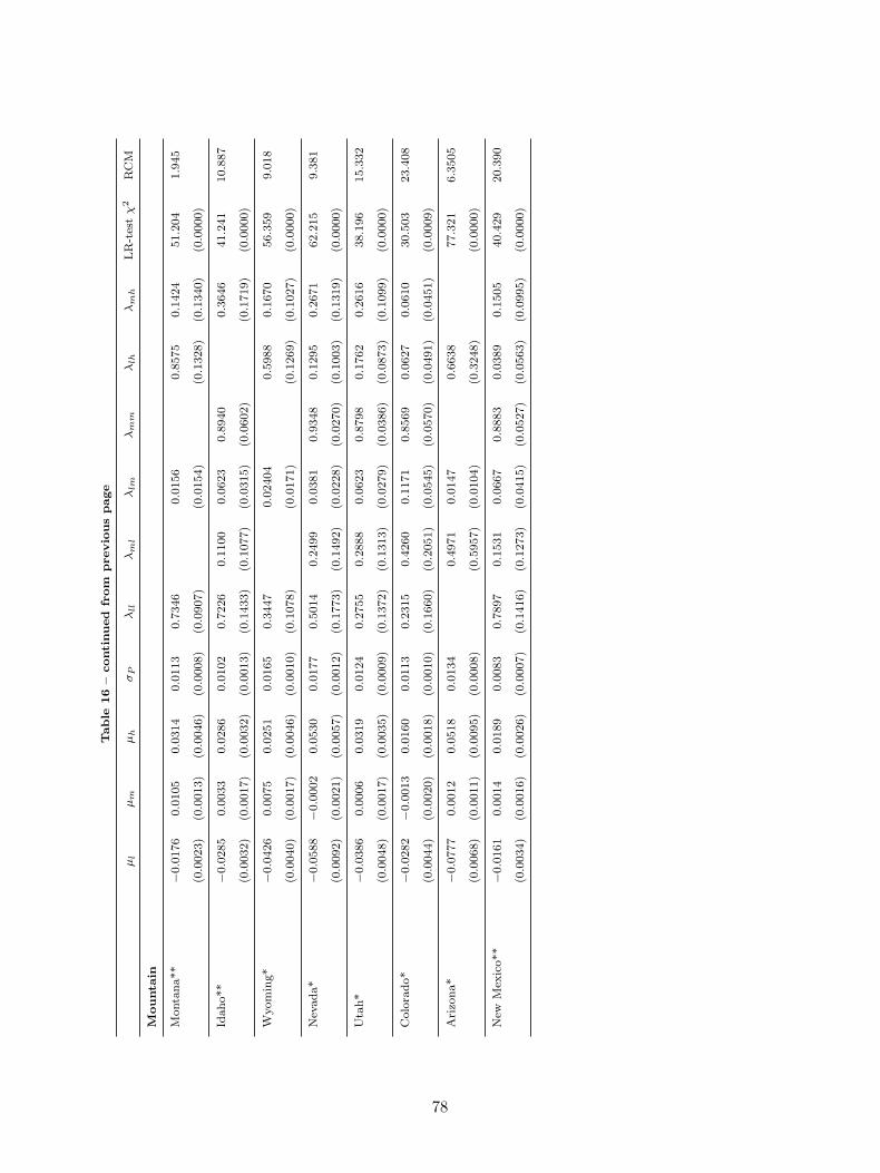
Tab

le16

–conti

nu

ed

from

previo

us

page

µl

µm

µh

σP

λll

λml

λlm

λmm

λlh

λmh

LR

-tes

tχ

2R

CM

Mou

nta

in

Monta

na**

−0.0

176

0.0

105

0.0

314

0.0

113

0.7

346

0.0

156

0.8

575

0.1

424

51.2

04

1.9

45

(0.0

023)

(0.0

013)

(0.0

046)

(0.0

008)

(0.0

907)

(0.0

154)

(0.1

328)

(0.1

340)

(0.0

000)

Idah

o**

−0.0

285

0. 0

033

0.0

286

0.0

102

0.7

226

0.1

100

0.0

623

0.8

940

0.3

646

41.2

41

10.8

87

(0.0

032)

(0.0

017)

(0.0

032)

(0.0

013)

(0.1

433)

(0.1

077)

(0.0

315)

(0.0

602)

(0.1

719)

(0.0

000)

Wyom

ing*

−0.0

426

0.0

075

0.0

251

0.0

165

0.3

447

0.0

2404

0.5

988

0.1

670

56.3

59

9.0

18

(0.0

040)

(0.0

017)

(0.0

046)

(0.0

010)

(0.1

078)

(0.0

171)

(0.1

269)

(0.1

027)

(0.0

000)

Nev

ad

a*

−0.0

588−

0.0

002

0.0

530

0.0

177

0.5

014

0.2

499

0.0

381

0.9

348

0.1

295

0.2

671

62.2

15

9.3

81

(0.0

092)

(0.0

021)

(0.0

057)

(0.0

012)

(0.1

773)

(0.1

492)

(0.0

228)

(0.0

270)

(0.1

003)

(0.1

319)

(0.0

000)

Uta

h*

−0.0

386

0.0

006

0.0

319

0.0

124

0.2

755

0.2

888

0.0

623

0.8

798

0.1

762

0.2

616

38.1

96

15.3

32

(0.0

048)

(0.0

017)

(0.0

035)

(0.0

009)

(0.1

372)

(0.1

313)

(0.0

279)

(0.0

386)

(0.0

873)

(0.1

099)

(0.0

000)

Colo

rad

o*

−0.0

282−

0.0

013

0.0

160

0.0

113

0.2

315

0.4

260

0.1

171

0.8

569

0.0

627

0.0

610

30.5

03

23.4

08

(0.0

044)

(0.0

020)

(0.0

018)

(0.0

010)

(0.1

660)

(0.2

051)

(0.0

545)

(0.0

570)

(0.0

491)

(0.0

451)

(0.0

009)

Ari

zon

a*

−0.0

777

0.0

012

0.0

518

0.0

134

0.4

971

0.0

147

0.6

638

77.3

21

6.3

505

(0.0

068)

(0.0

011)

(0.0

095)

(0.0

008)

(0.5

957)

(0.0

104)

(0.3

248)

(0.0

000)

New

Mex

ico**

−0.0

161

0.0

014

0.0

189

0.0

083

0.7

897

0.1

531

0.0

667

0.8

883

0.0

389

0.1

505

40.4

29

20.3

90

(0.0

034)

(0.0

016)

(0.0

026)

(0.0

007)

(0.1

416)

(0.1

273)

(0.0

415)

(0.0

527)

(0.0

563)

(0.0

995)

(0.0

000)

78