working paper no. 225 foreign portfolio investment flows to india: determinants and analysis pami...

CDE February 2013

FOREIGN PORTFOLIO INVESTMENT FLOWS TO INDIA

: DETERMINANTS AND ANALYSIS

Pami Dua Email:[email protected]

Department of Economics Delhi School of Economics

Reetika Garg

Email: [email protected] Department of Economics Delhi School of Economics

Working Paper No. 225

Centre for Development Economics Department of Economics, Delhi School of Economics

1

FOREIGN PORTFOLIO INVESTMENT FLOWS TO INDIA: DETERMINANTS AND ANALYSIS

Pami Dua

Department of Economics, Delhi School of Economics,

University of Delhi, Delhi-110007, India

Email:[email protected] and

Reetika Garg Department of Economics,

Delhi School of Economics, University of Delhi, Delhi-110007, India

Email:[email protected]

Corresponding Author: Reetika Garg, Research Scholar, Department of Economics, Delhi School of Economics,

University of Delhi, Delhi 110007. Telephone: +91-11-27666533-35, 27666703-05 Ext.157 Fax: +91-11-27667159

Email:[email protected]

2

Foreign Portfolio Investment Flows to India: Determinants and Analysis

PAMI DUA

and

REETIKA GARG

ABSTRACT

This paper analyses the determinants of portfolio flows to India for the period October 1995 to October

2011. The determinants of disaggregated component of portfolio flows (FPI) i.e. foreign institutional

investment flows (FIIs) and investment flows received through American/Global depository receipts

(ADR/GDRs) are also examined. The determinants are based partially on the portfolio balance model in

which capital flows in an emerging economy are determined through an arbitrage condition. These

include domestic stock market performance, exchange rate, reserves to import ratio, interest rate

differential, volatility in exchange rate, domestic output growth, foreign output growth and emerging

market equity performance.

The results indicate that domestic stock market performance, exchange rate and domestic output growth

are the most important determinants of both FII and ADR/GDR flows. Emerging market equity

performance, interest rate differential and volatility in exchange rate influence FII flows but not the

investment flows received through ADR/GDRs. Moreover ADR/GDR flows are influenced by foreign

output growth, but this is not so for the FII flows. Since FIIs have been the most dominant component of

aggregate portfolio flows, therefore as expected, the results for aggregate portfolio flows are similar to FII

flows.

Keywords: FPI, FII, ADR/GDRs, Portfolio balance framework, ARDL model

3

1. INTRODUCTION

The international flow of capital is expected to benefit both the source as well as the host country.

However, the historical and recent financial crises have also brought into focus the fact that these flows

can expose the countries to new risks. Hence it is important to understand the risks associated with these

flows and the factors that drive flows into India, so that policy reactions can be formulated in advance to

avoid any imbalances arising out of extremely high capital inflows or sudden reversal of capital flows in

future, whatever the case may be.

The recent volatility in capital flows, especially when periods of high capital inflows were

followed by periods of huge reversal in these flows, has posed macroeconomic challenges to countries

across the world. India has not remained untouched by the developments in the global financial markets

due to greater linkages of the Indian markets with the international markets. The recent volatility in

capital flows to India can mainly be attributed to volatility in foreign portfolio investment flows and

especially the foreign institutional investment flows. Hence it is important to analyse the determinants of

portfolio flows in this uncertain global scenario.

Foreign portfolio investment (FPI) flows have been the most volatile component of capital flows

in India and play an important role in determining the overall balance of payments. During the Asian

crisis as well as during the recent sub-prime crisis, it was the huge reversal of FPI flows that led to

deterioration in the overall balance of payments. This is because by their very nature FPI flows do not

involve a long lasting interest in the economy. The ultimate aim of FPIs is to ensure profits and risk

diversification.

This study examines the determinants of portfolio flows to India in the light of increasing

volatility in FPI flows which is due to uncertainty in the global scenario in recent times. This is done by

using the determinants suggested by a theoretical model, initially proposed by Fernandez- Arias (1996)

and Fernandez- Arias and Montiel (1995), where portfolio flows have been modeled using a zero

4

arbitrage condition. According to the model expected return from investing in the host country, adjusted

for credit worthiness of the country should be equal to the opportunity cost i.e. returns from investing in

home country. The model therefore suggests that capital flows are a function of economic factors in the

host and the source country and also of the factors that influence creditworthiness of host country.

These factors include domestic stock market performance, exchange rate, foreign exchange

reserves to imports ratio, volatility in exchange rate, interest rate differential and domestic and foreign

output growth. In addition to the factors suggested by the theoretical model, other factors that are

considered important are also included in the empirical model. This includes the effect of the stock

market performance of emerging markets in general, on portfolio flows received by India is captured by

emerging market MSCI index.

The disaggregated components of FPI flows i.e. determinants of Foreign Institutional Investment

flows (FIIs) and American/Global Depository Receipts (ADRs/ GDRs) which have been the major

components of FPI flows to India are also analyzed. It is important to do so in order to assess whether

different components of portfolio flows are driven by the same or different factors.

The results indicate that a well performing domestic stock market, an appreciating exchange rate

and strong domestic economic growth attracts portfolio flows. Greater volatility in the exchange rate

discourages these flows. If the overall stock market performance of emerging markets in general is good

then the flows received by India decline indicating that India competes with other emerging economies in

terms of receiving portfolio flows. A higher interest rate differential between domestic and foreign

interest rates attracts FPI flows. The results relating to FII flows are same as that of aggregate FPI flows.

For ADR/GDRs, domestic stock market performance, exchange rate, domestic as well as foreign output

growth, are observed to be the most significant determinants. It is observed that reserves to import ratio,

which measures creditworthiness of India, does not influence any component of portfolio flows, in time

series framework.

5

This paper makes an important contribution to the literature related to FPI flows to India. Most of

the literature that analyses the determinants of portfolio flows (FPI) to India has concentrated on the FII

component only. ADR/ GDR flows have not received much attention despite the fact that the Indian

corporate sector has increasingly used ADR/GDR mechanism to raise foreign capital. This study thus

examines the macroeconomic determinants of not only FII but also ADR/GDR flows to India in order to

fill the existing gap in the literature.

Furthermore, this study examines a wider set of potential determinants of FII flows to India

compared to other studies pertaining to the Indian economy such as Chakrabarti (2001), Kaur and Dhillon

(2010), Rai and Bhanumurthy (2004), Srinivasan and Kalaivani (2013). While the study by Gordon and

Gupta (2003) includes a wide range of determinants of portfolio flows, it uses the OLS methodology that

may yield biased and inconsistent estimates if the regressors are endogenous. This study follows the

ARDL approach to cointegration for estimating the long-run coefficients which overcomes such

problems. The long-run coefficients are unbiased and the t-tests are also valid, even if the regressors

included in the specification are endogenous (Harris and Sollis 2003)

The following section discusses the trends in the portfolio flows to India. Section 3 presents the

theoretical portfolio balance model which suggests some of the factors determining financial flows.

Section 4 discusses the empirical model and section 5 presents the data sources and methodology, used

for estimation. Section 6 discusses the empirical results and section 7 concludes.

2. TRENDS IN DIFFERENT COMPONENTS OF PORTFOLIO FLOWS TO INDIA

To understand the volatile nature of FPI flows, it is important to know what constitutes these

flows. According to UNCTAD (1999) portfolio investment involves transfer of financial assets by way of

investment by resident individuals, enterprises and institutions in one country in securities of another

country, either directly in the assets of the companies or indirectly through financial markets. The main

aim of the investor is to benefit from capital gains or to reduce the risk of the portfolio that the investor

6

holds by diversifying internationally. The different components of FPI flows are Foreign Institutional

Investors1, Global/American Depository Receipts2 and offshore funds.

In 1992, the Indian government allowed the foreign investors to invest in the financial markets of

the country. To be able to invest in Indian financial markets, the FIIs must be registered with the

Securities and Exchange Board of India (SEBI). SEBI prescribes certain norms which are to be followed

by the FIIs for registration, for example they are required ensure compliance with Foreign Exchange

Management Act 1999 for which they need permission from RBI; they are required to pay registration

fees; etc.. Overtime, the regulatory measures of SEBI have become liberal, which has increasingly

encouraged FIIs to invest in India. However, in addition, the role of robust growth performance of the

Indian economy and the resilience of the country in times of global crisis in making India one of the most

favoured destinations for investment cannot be overlooked. Presently, the insurance companies, banks,

hedge funds, mutual funds, asset management companies and pension funds form the majority of FIIs

investing in India3.

American/Global Depository Receipts provide a mechanism of indirect listing of Indian

companies in foreign stock exchange. The Indian company that wants to get listed indirectly in the

foreign stock exchange, deposits its shares in a bank in that country. The bank then issues receipts against

these shares, which are sold to the residents of that country. These receipts are also listed in the stock

exchange of that country and are bought and sold like other instruments. The prices of these are also

1 FIIs are those institutions, enterprises or organizations that invest in the financial markets of the other country.

2 American/Global Depository Receipts are instruments that are used by NRIs and foreign nationals for investing in

Indian companies.

3 Currently there are 1506 FIIs registered with SEBI out of which 56% belong to Mauritius (The Times of India May

12 2012). This may be because the funds from other countries are also mobilized to India via Mauritius to ensure tax

benefits which accrue due to the Double Tax Avoidance Agreement (DTAA) between India and Mauritius.

7

determined by the market forces. If the receipts are traded in American markets then they are called

American Depository Receipts and if these are traded in markets of countries other than America, then

they are called Global Depository Receipts.

An alternative way of investment in Indian companies by NRIs and foreign nationals would be if

the companies directly get listed in the stock exchange of the foreign country to which these people

belong or they come and invest in Indian markets directly. Both these methods involve a lot of restrictions

and have great costs. Investment through ADR/GDRs helps to overcome these limitations and hence is

preferred over the aforesaid methods.

Investment in Offshore financial funds i.e. those funds that are supposed to provide tax benefit to

the investor are also included under the category of portfolio investment flows. In India a few companies

that have offshore mutual funds are Reliance, Kotak and TATA.

FIIs have been the most dominant component in the history of aggregate portfolio flows to India.

The cumulative FII investment has increased consistently from 1.6 billion dollars in 1993-94 to

approximately 127.8 billion dollars till December 2011, with the only exception of a decline to 59 billion

dollars in 2008-09 from 68.9 billion dollars in 2007-08(SEBI HoS 2011).

In Figure 1, if we focus on the annual trends in net investment inflows through FIIs, it can be seen

that after 1992-93 when FIIs were allowed to enter the capital markets of India, FII flows started rising.

Till 1996-97 these flows kept rising, however, in 1997-98 and 1998-99 there was a reversal in FII

investment due to the impact of the Asian crisis. Although Indian economy was not directly involved in

the crisis, and the intervention by RBI in the currency market as well as imposition of capital controls was

used to insulate the Indian economy from the crisis (Dua and Sinha 2007), still the foreign investment

flows to the Indian economy declined, specially the FIIs. This was mainly due to the contagion effect i.e.

deterioration of investor confidence in the East and South-east Asian region. However as compared to

other East Asian countries, the magnitude of adverse impact on India was small and short lived.

8

In 1999-2000 FII flows to the Indian economy revived but again dipped to 2.77 billion dollars in

2002-03. This was mainly due to the sluggish performance of the Indian stock markets, as well as the

credit rating downgrade of the Indian economy by the international credit rating agencies. In the

following year in 2003-04, FII flows shooted up to 10.9 billion dollars which was mainly the result of an

increase in the limit of investment by FIIs in the securities of the Indian companies and increase in the

number of sectors in which the investment could be made as well as allowing FIIs to invest in the

derivatives market.

The overall trend in FPI flows imitates the trend in FII investment, with the peaks and troughs of

both the flows coinciding with each other in every single instance. In 2008-09, it was the huge reversal in

FII flows that created havoc in the Indian financial markets and led to a sharp decline in the total portfolio

investment flows to India. The magnitude of decline was so immense that its effect on the overall balance

of payments was also felt. Although the decline in investment received through ADR/GDRs was also

seen but the magnitude was not large. A similar role of FIIs during the Asian crisis was also seen with the

sharp reversal in FIIs leading to a decline in total portfolio flows despite a rise in investment received

through ADR/GDRs during the Asian crisis.

In 1992 Indian companies were allowed to raise capital by issuing depository receipts in the

world financial markets. In 2001-02 Indian government announced several liberal measures relating to

portfolio flows like increase in investment limit by FIIs from 40-49 percent and allowing two way

fungibility of ADRs and GDRs. On the other hand international financial markets were also taking

measures to attract firms in the emerging markets to list on their stock exchanges. Both these

developments resulted in investment flowing into India through the ADR/GDR route.

Initially in the 1990s Indian firms refrained from listing in the US stock exchanges because of the

stringent accounting standard requirements of US GAAP and SEC. The most attractive destination of the

Indian firms was London Stock Exchange and Luxemburg Stock Exchange.

9

However, as observed by Pagano et. al. (2002), poor liquidity in the European stock exchanges

made Indian companies change their preferences and they started listing on US stock exchanges. This was

also because, overtime, Indian companies improved their accounting standards, reflecting greater

transparency, which allowed these firms to list in the US stock markets as well. Initially most of the

Indian companies listing in the US, listed on the NASDAQ and then later on NYSE as well because of the

stricter norms of NYSE.

The share of FIIs in total FPI flows has always been higher than the share of investment flows

received through ADR/GDRs since 1996-97, except in 2002-03 and in 2006-07. The share of ADR/GDR

flows has declined overtime but this does not mean that ADR/GDR flows are insignificant component of

FPI flows. In 1996-97 the share of ADR/GDR flows was 41 % and that of FII flows was 58%. In 2007-

08 the share of ADR/GDR flows was 24% and that of FII flows was 75%. In 2009-10 FII flows

accounted for 89% of the total flows while ADR/GDR flows were 10% of the total flows. Offshore funds

have always been a minor portion of the total portfolio flows, however in the recent years since 2008-09,

India has not been receiving any investment on account of offshore funds.

In absolute terms, as can be observed from Figure 1, there has been a surge in investment flows

received through ADR/GDRs from 2004-05 onwards, while the magnitude of FII flows increased

considerably after 2002-03.

3. THEORETICAL MODEL

(a) Portfolio balance framework

The empirical model in this paper draws from the factors suggested by the theoretical model

which is based on the fact that foreign investors exploit all the possibilities of arbitrage across the home

and the host country. In addition to the factors suggested by the theoretical model, the empirical model

will include additional variables that may influence financial flows.

10

The literature on the theoretical model of capital flows in portfolio balance framework mainly

includes the model developed by Fernandez- Arias and Montiel (1995) and extended by Taylor and Sarno

(1997) and Mody, Taylor and Kim (2001). This model analyses the effect of domestic (pull) and global

(push) factors on capital flows. Pull factors represent country specific investment risk and returns which

attract foreign investment and push factors represent global liquidity and other factors that push

investment towards emerging economies. The model bifurcates the domestic factors into those that

operate at country level and those that operate at asset / project level. Assume that capital flows are

represented by transactions in different types of assets s = 1…….n. The expected return by investing in an

asset of type i in an emerging economy comprises of two elements. First is the expected return from the

project ( sG ) and the second is an adjustment factor for sG depending on credit worthiness of the country

( sC ).

The expected return from the project is of function of vector of net capital flows (F) going into

each project and the domestic economy environment (g). The adjusting credit worthiness factor is a

function of stock of capital ( FSS 1 ) and other factors reflecting credit worthiness of the emerging

economy (c).

The stock of capital S is the vector of each of period stocks of liabilities which is the sum of

initial stocks of liabilities and current net capital inflows.

Now the foreign investor will consider the opportunity cost of assets of type )( sVs . This is the

return the foreign investor gets by investing in his own economy. sV is a function of the stock of capital

)( 1 FSS and the financial and economic opportunities in the source country (v).

Note that g and c represent pull factors and v represents push factors.

The arbitrage condition is thus given by

sG (g,F) sC (c, FS 1 ) = sV (v, FS 1 )

11

Assume that sG , sC & sV are increasing functions of g, c & v respectively. The above equation

can be solved for equilibrium vector of net capital flows F* which can be expressed as:

F* = F* (g, c, v, 1S )

This gives the effect of change in economic factors in host country (g) and source country (v) and

also the effect of factors that influence creditworthiness of host country (c), on changes in capital flows.

To capture the effect of economic factors in the host country (g) domestic stock market

performance, exchange rate, domestic interest rate, domestic output growth and volatility in exchange rate

are included. For the source country factors (v), foreign interest rate and foreign output growth are

included. As a measure of creditworthiness (c) reserves to import ratio is included in the empirical model.

(b) Other Factors

While diversifying globally, foreign investors can either invest in emerging markets or they can

invest in financial markets of the industrialized countries. According to Buckberg (1996) investors

follow a two step process in deciding capital allocation. Firstly, the total capital to be invested in

emerging markets is determined and then a part of that capital is allocated to each of the emerging

market depending on returns. This implies that if total capital allocated to emerging markets is

high, then each emerging economy has a higher probability of receiving greater amount of capital.

Alternately, it is also important to view different emerging economies as competitors to

each other, where each economy is trying its best to receive a greater share of foreign investment.

In this case, once the foreign investor decides the total amount to be invested in all the emerging

economies taken together, then a higher share will be received by a particular emerging economy

only at the cost of another.

Thus emerging market stock returns are also included in the empirical estimation in

addition to the variables suggested above.

12

4. EMPIRICAL MODEL

The portfolio balance framework categorizes the determinants of portfolio flows into factors that

affect returns from investment in the host country, factors that affect creditworthiness of the host country

and factors that affect returns from investment in the home country. Variables that capture these factors

alongwith an indicator of emerging market stock performance are used to estimate the empirical model.

FPI/FII/ADR = f (S, e, R/M,MSCI, i-i*, y, y*, Vol (e))

where the dependant variables are foreign portfolio investment inflows (FPI), foreign institutional

investment inflows (FII) and American/ Global Depository Receipts (ADR), all three denominated in

billions of US dollars.

The independent variables include

Domestic stock market performance - BSE Sensex (S)

Exchange Rate - Nominal effective exchange rate 36 country export based (e).

Creditworthiness indicators – reserves to import ratio (R/M)

Regional factor – Morgan Stanley Capital International Emerging Markets Net Index (MSCI)

Excess of Domestic Interest Rate over Foreign Interest Rate - 3 month Treasury bill rate for India

- 3 month LIBOR (i-i*)

domestic output growth - m-o-m IIP growth of India (y)

foreign output growth - m-o-m IIP growth of OECD countries (y*)

Exchange Rate Volatility- square root of estimated variance in nominal effective exchange rate

from GARCH model (Vol(e))

The domestic stock market returns can influence portfolio flows in a positive way when foreign

investors are said to be chasing the returns. In the Indian context a positive relation is observed by

Aggarwal (1997), Chakrabarti (2001), Rai and Bhanumurthy (2004). However if the influence is negative,

it would be a case of foreign investors buying (selling) when domestic stock returns are low (high), with

the expectation that returns will rise (fall) in future (Gordon and Gupta 2003).

13

In a world of flexible exchange rate, capital can earn a return not only through yields on

assets, but also through a change in exchange rate overtime. Appreciation of currency of the host

country, intertemporally, is an additional avenue of gaining returns for foreign investors. In the

Indian context, exchange rate is found to be significant in explaining portfolio flows especially FII flows

(Chakrabarti 2001, Gordon and Gupta 2003, Bhattacharya, Bhanumurthy, Chakravarty and Rai 2003).

Reserves to import ratio is included as a measure of availability of sufficient liquidity in India, so

that in the event of withdrawal of funds by the investors, India doesn’t default on the payments. Higher

value of this ratio is an indicator of availability of sufficient stock of reserves to meet short run

obligations and hence is a measure of credit worthiness of the country or sovereign risk. It is expected that

countries with sufficient amount of reserves (able to cover for imports) are perceived to be credit worthy

and the probability of their defaulting is less. Thus it is hypothesized that the periods when India has

sufficient reserves will coincide with greater flows.

Emerging market stock returns captured by MSCI Index4 is used to capture regional effects and it

determines the allotment of capital by foreign investor to emerging market economies. If the index is

higher then the allotment of capital by foreign investor to emerging market economies is higher and hence

the proportion allotted to the emerging economy like India will also be higher. This would mean that the

income effect is higher and flows to India are complementary to flows received by other emerging

markets. Alternately, if India is competing with other emerging economies in receiving the financial

4 The Morgan Stanley Capital International (MSCI) Emerging Markets Net Index is a free float-adjusted market

capitalization weighted index which measures equity market performance of emerging markets. The MSCI

Emerging Markets Index consists of 21 emerging market country indices. These include 5 American countries

(Brazil, Chile, Columbia, Mexico and Peru); 8 European, Middle East and African countries (Czech Republic,

Egypt, Hungary, Morocco, Poland, Russia, South Africa and Turkey); and 8 Asian countries (China, India,

Indonesia, Korea, Malaysia, Philippines, Taiwan and Thailand)

14

flows, then a higher value of the index would mean lesser magnitude of flows received by India and vice-

versa. This would mean that the substitution effect dominates.

Interest rate differential between the host and the source country also determine portfolio

flows. The traditional open economy macroeconomic models proposed by Mundell and Fleming

suggest that in a world where capital is mobile and exchange rates are fixed, capital flows occur so

as to restore interest parity, i.e. capital moves in or out of the country till the domestic and foreign

interest rates equalize. Investors invest their capital wherever the interest rates adjusted for risk are

higher. Verma and Prakash (2011) find that FDI and FII flows to India for the period 2000-01 to

2009-10 are not sensitive to interest rate differentials5.

Domestic output growth is used to indicate the soundness of macroeconomic and institutional

fundamentals of the host country, which are very important in attracting capital flows. A higher economic

growth in India indicates rapidly expanding economic activity (Dua and Rashid 1998) which in turn

would mean greater profitability from investing in the Indian corporate sector. Index of Industrial

Production is an appropriate reflection of these.

Foreign output growth which is measured by the growth of OECD industrial production

represents the profitability of investment in the corporate sector in OECD countries. With regard to

foreign output growth, it is argued in the literature that a slowdown in the growth of industrialized

countries (most importantly US), increases liquidity in international markets, leading to greater capital

flows to emerging market economies. Verma and Prakash (2011) for the period 2000-01 to 2009-10

find that OECD output growth is positively related with capital flows to India

Volatility in exchange rate is expected to have negative impact on capital flows to India

especially FPI flows. A higher volatility represents a higher degree of uncertainty in the returns received

5 Interest rate differential measured as the difference between interest rate on NRI deposits and six month

LIBOR.

15

by foreign investor. This is because exchange rate plays an important role in deciding the returns in terms

of home currency of the investor. Persson and Svensson (1989) observe that increased exchange rate

variability has negative impact on international trade and capital flows.

The impact of recent subprime crisis that originated in US, but affected the real and financial

flows across the globe, is capture through a dummy. When global liquidity is affected due to any given

exogenous reason, the flow of financial investment to emerging economies gets hit. Thus it is necessary to

control for such effects.

5. DATA AND METHODOLOGY

The main sources of the data used in the analysis are Handbook of Statistics and Current Statistics

of RBI, International Financial Statistics of IMF and Federal Reserve Bank. Net portfolio inflows, FII

flows and ADR/GDR flows denominated in US $ billion are taken as the dependent variable.

Domestic stock market performance is measured by the monthly average of the BSE sensitivity

index. Exchange rate is defined as the nominal effective exchange rate 36 country (export based)6.

Interest rate differential is defined as the difference between 3 month Treasury bill rate for India and 3

month LIBOR7. Domestic output growth is defined as the annual growth rate of index of industrial

production for India. Similarly foreign output growth is measured by annual growth rate of index of

industrial production for OECD countries. Both the series are calculated as the difference between

logarithm of index of a particular month and the twelfth lagged month. This also helps to remove the

seasonality in the IIP series if there exists any.

Reserves to imports ratio is calculated as the total reserves divided by the imports, both

denominated in US million dollars. Emerging market MSCI index is obtained from the

6 The results are robust to the use of 36 country trade based nominal effective exchange rate.

7 Alternately it can also be defined as the difference between 3 month Treasury bill rate for India and 3 month

Treasury bill rate for US. The results are robust to this definition.

16

www.mscibarra.com. Volatility in exchange rates is calculated using the GARCH method8. The goal of

GARCH method is to provide a volatility measure similar to a standard deviation.

According to the ARCH model, variance of a variable at time t is a weighted average of the

squared residuals of the previous time period (t-1, t-2,…). The weights are estimated in such a way so that

the observations in the more recent past get higher weights compared to observations far away in the past.

GARCH model is a generalization of the ARCH model where variance of a variable at time t is a

weighted average of not only the squared residuals but also the variance of residuals in the previous time

period (t-1, t-2,…). The residuals are calculated by fitting an appropriate univariate ARMA model on the

variable. GARCH(p,q) model can be represented as:

tttt eyEy )|( 1 and

q

jjtj

p

iitit e

1

2

1

20

2

(a) Dickey-Fuller Test with GLS Detrending (DFGLS)

To test if a series ty contains a unit root or whether it is non-stationary, Dickey Fuller

Generalised Least Squares Test is employed. If we chose to include a constant, or a constant and a linear

time trend, in the ADF test regression, then for these two cases, Elliot, Rothenberg, and Stock (1996)

propose a simple modification of the ADF tests in which the data are detrended so that the effect of

constant and trend need not be captured by the ADF test equation, explicitly.

For this Elliot, Rothenberg, and Stock (1996) define a quasi-difference of yt, which is regressed

on the quasi-differenced xt, where xt includes the constant or a constant and trend. The residual series of

this regression is the GLS detrended data ytd.

8 To check for robustness, the 3 month moving average standard deviation in nominal effective exchange rate was

alternatively used to measure volatility in nominal effective exchange rate, and the results are qualitatively similar.

17

The DFGLS test involves estimating the standard ADF test equation, after substituting the GLS

detrended ytd for the original yt:

t

p

i

diti

dt

dt yyy

1

11

Note that since ytd are detrended, we do not include the constant or trend in the DFGLS test

equation. As with the ADF test, we consider the t – ratio for α from this test equation. While the DFGLS

t-ratio follows a Dickey-Fuller distribution in the constant only case, the asymptotic distribution differs

when both a constant and trend are included. Elliot, Rothenberg, and Stock (1996) simulate the critical

values of the test statistic in this latter setting. The null hypothesis is rejected for values that fall above the

critical value band.

(B) Autoregressive Distributed Lag (ARDL) Model

The cointegration methods proposed by Engle and Granger (1987) based on residuals and

Johansen (1991, 1995) and Johansen-Juselius (1990) based on maximum likelihood estimation are

applicable only if all the series are integrated of the same order. However, while carrying out any

macroeconomic study and identifying the relation between any two or more time series variables it may

be the case that they are not integrated of the same order. In that case, one possibility is that the series that

are integrated of higher orders should be differenced so that all the variables in the analysis are integrated

of the same order, and then the conventional cointegration methods are applied. But, in such a case, the

interpretation of coefficients sometimes loses its meaning. To overcome this limitation, the autoregressive

distributed lag (ARDL) approach to co-integration was proposed by Pesaran and Shin (1999) and Pesaran,

Shin and Smith (2001). This method is applicable irrespective of the fact that the variables included in the

analysis are I(0) or I(1) or fractionally integrated.

The ARDL method cannot be applied if either of the variables is I(2) so it is still important to

check for unit root to make sure that none of the variables are integrated of order higher than one.

18

The estimates based on ARDL are highly consistent and inferences regarding the long run

parameters based on standard normal asymptotic theory are valid.

(c) Bounds Testing Approach

To test whether there exists a long run relation between the variables, when all the variables are

integrated of different order i.e. I(0) or I(1), bounds testing approach is used. This involves testing the null

hypothesis of 0......21 k against the alternative hypothesis of

0.......21 k in the following equation

titk

m

ikiit

m

ii

it

m

iiit

m

itkktttt

xx

xyxxxycy

,1

,21

2

,11

11

1,1,221,111

.........

.......

The calculated F-statistic has a non standard asymptotic distribution of under the null hypothesis

of no long run relationship between the variables, irrespective of whether the variables are I(0) or I(1) or

fractionally integrated. Pesaran and Pesaran (1997) have two sets of asymptotic critical values for the F-

statistic. One is the lower bound critical value which assumes that all variables are integrate of order zero

i.e. I(0). The other is the upper bound critical value which assumes that all variables are I(1). If the

calculated F-statistic is greater than the upper bound critical value then the null hypothesis of no long run

relationship is rejected. If the computed F-statistic falls below the lower bound critical value, then the

null hypothesis of no long run relationship is not rejected. If the calculated F-statistic falls within the

lower and upper bound critical values, then the result is inconclusive.

(d) Estimation of Long-Run Relationship

The Augmented ARDL (p, q1, q2, …… qk) is given by the following equation (Pesaran and

Pesaran, 1997; Pesaran, Shin and Smith, 2001)

ttiti

k

iit wxqLypL

'

1

),(),( nt ,,.........1

19

where

kLLLqL

LLLpL

iq

iqiiiii

pp

i

i...,2,1.......),(

........1),(2

21

221

yt is an independent variable, L is the lag operator such that Lp yt = yt-p, wt is the s 1 vector of the

deterministic variables such as the intercept term, time trends, dummies or exogenous variables with fixed

lags. itx represents i th independent variable where i = 1, 2, ……, k where lag order of ith variable is qi .

This equation is first estimated through OLS for p=0,1,2, .....m and qi=0.1.2....m where m is the

maximum lag chosen. All the possible ARDL models with all the possible permutations of the lag

structure are estimated and the total number of ARDL models estimated are (m+1)k. The appropriate lag

structure is chosen based on different criterion such as AIC, SBC and HQC in such a way so that there is

no remaining serial correlation in the chosen model. Once the appropriate lag structure of the model is

chosen, the long-run slope coefficients of the endogenous variables are estimated as follows:

Φ

),1( ii q

),1(ˆ pki ,...,2,1

where p̂ and iq̂ , i = 1, 2, …, k are the selected (estimated) values of p̂ and iq̂ , i = 1, 2, …, k

Φi gives the long run impact of xit on yt.

The long-run coefficients of the deterministic variables included in the model are estimated by:

p

ki

qqqp

...1

),...,,,(

21

21

Symbols with hat (^) denote the OLS estimates for the selected ARDL model.

When the selected ARDL ( kqqqp ˆ...,ˆ,ˆ,ˆ 21 ) model is written in terms of lagged levels and the first

difference of yt, x1t, x2t,, xkt and wt, we get the error correction model (ECM) which is as follows:

20

tjti

k

i

q

jijt

p

jjtit

k

iittititt xywxwxypy

t

,1 1

*1

1

1

*'

11

'1

))(,1(

titit wxy '

is defined as the error correction term and is interpreted as the speed of

adjustment to the equilibrium when the model is given a shock. and are defined as :

i 1,2, … . p 1

, j 1,2, … . q 1

According to Pesaran and Pesaran (1997) and Pesaran, Shin and Smith (2001) the first step in the

estimation of long run relation through the ARDL approach is to test whether there exists a long-run

relationship amongst the variables in the model to be estimated. For this the bound testing approach

described above is used. If there exists a long run relationship, then the second step involves estimating

the long-run and short-run coefficients of the given equation.

The error correction model derived from the ARDL framework can also be used to test for

Granger causality. This can be done by testing the statistical significance of the error correction term

using a t-test, or by testing the joint significance of the sum of lags of each explanatory variables using F-

test. Alternatively a joint test of all the aforesaid terms can be conducted using F-test.

6. EMPIRICAL RESULTS

(a) Results of the Unit Root Test and the Bounds Test

The DFGLS unit root tests 9 suggest that Indian output growth, foreign output growth and

volatility in exchange rate are stationary. All the other variables i.e. net FPI inflows, net FII inflows, net

9 Augmented Dickey-Fuller Test (Dickey and Fuller 1979,1981), Phillips-Perron Test (Phillips and Perron 1988),

and the Kwiatkowski, Phillips, Schmidt, and Shin Test (Kwiatkowski, Phillips, Schmidt, and Shin 1992) were also

conducted and all of them give the same result as the DFGLS Test

21

ADR/GDR flows, domestic stock market index, exchange rate, emerging market stock returns index,

reserves to imports ratio and interest rate differential are integrated of order one. Since the variables under

consideration are a mix of I(0) and I(1), hence the ARDL method was found suitable for estimation.

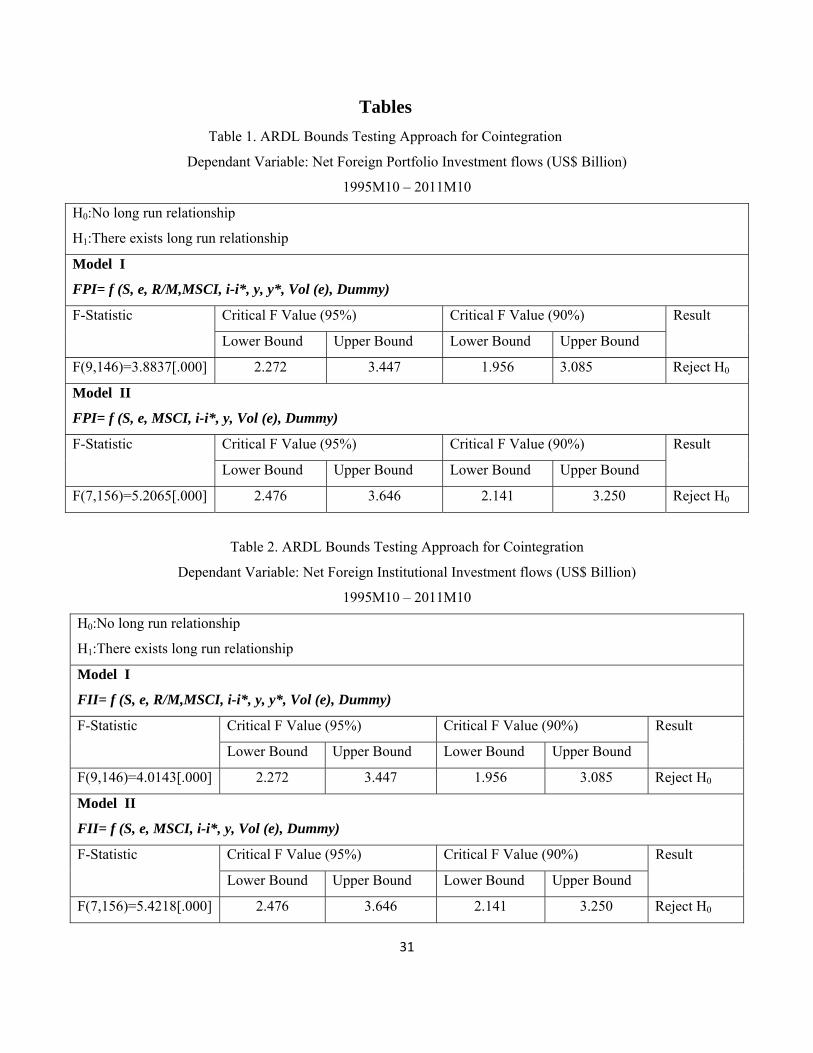
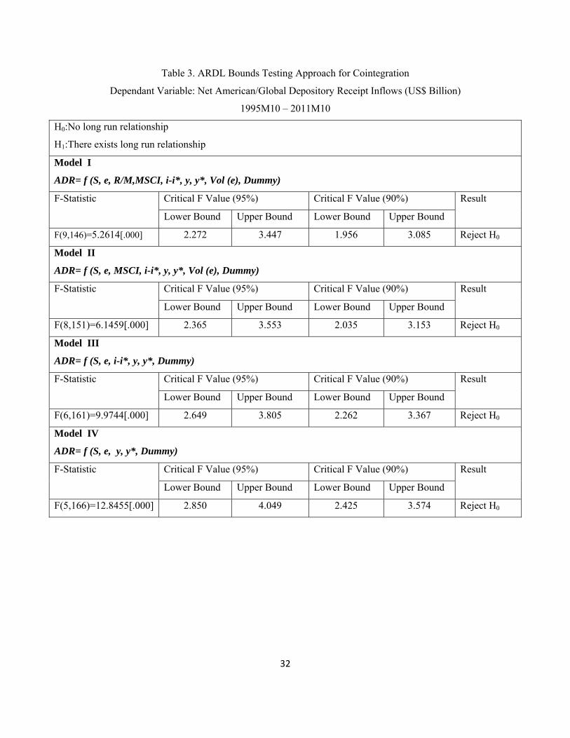
The first step is to check for cointegration between the variables using the ARDL bounds test

suggested by Pesaran, Shin and Smith (2001). The null hypothesis of no long run relation of domestic

stock market performance, exchange rate, emerging market equity performance, reserves to import ratio,

interest rate differential, domestic output growth, foreign output growth and volatility in exchange rate

(calculated through GARCH method10) with FPI, FII and ADR/GDR flows was tested. Note that in the

first specification of FPI, FII and ADR/GDR flows all the variables were included, but in the subsequent

specifications, depending on the results, a few variables were excluded. However, for each specification

bounds test was conducted to ensure that long run relationship between the variables included in the

respective specification existed. A maximum lag value of four was used for implementing the test.

The dummy variable for crisis was also included in the FPI and FII specifications, since it was

observed that these flows were affected the most during the recent subprime crisis. For ADR/GDR a

dummy variable to control for three outlier observations was included. For all the specifications, the null

hypothesis is rejected, as the calculated F-statistic lies above the upper bound critical F value at 95%

(Table 1, 2 & 3).

Once the bounds test ensures the presence of long run cointegration between the variables, the

next step is to estimate the ARDL model and obtain the long run coefficients and then perform granger

causality tests based on the short run error correction model. The optimal lag length for the variables is

chosen such that there is no residual serial correlation in the underlying model.

10 The results are qualitatively similar even if we use the 3 month moving average standard deviation in NEERE as

the definition of volatility in nominal effective exchange rate.

22

(b) Aggregate Foreign Portfolio Investment Inflows and Foreign Institutional Investment Inflows

As noted earlier, the decomposition of aggregate FPI flows shows that FII flows are a dominant

component of FPI flow and the peaks and the troughs in total FPI flows closely matches with that in FII

flows (Figure 1), hence as expected, the estimation results of aggregate FPI flows is quite similar to that

of FII flows (Table 4 &5).

For all the specifications of FPI and FII (Table 4 &5), the coefficient on domestic stock market

performance is found to be positive and statistically significant (at 1% level of significance) indicating

that well performing domestic stock markets attract portfolio flows and FII flows to India. Similarly the

coefficient on exchange rate is positive and significant in all the specifications indicating that an

appreciating exchange rate attracts greater flows (FPI as well as FII) to India. This is because an

appreciating exchange rate provides an additional source of returns to foreign investors. The impact of

exchange rate on aggregate portfolio flows was stronger relative to FII flows, both in terms of magnitude

and statistical significance.

The impact of improvement in performance of emerging market stocks has a negative impact on

FII as well as aggregate FPI flows to India. This implies that when the overall returns from investing in

emerging market stocks in general increases, foreign investment received by India decreases. Thus

substitution effect dominates the income effect with regard to FPI and FII flows. In other words, when

emerging markets as a whole perform better, then income effect would mean greater allocation of funds

to emerging markets by foreign investor, because of which the probability that greater funds are allotted

to each emerging economy increases. However, there is also a possibility of substitution of investment

flows between these emerging economies, because all of them compete with each other for receiving

these flows. In case of India, the former effect gets dominated by the latter.

The differential between domestic and foreign interest rates has a positive association with

portfolio and FII flows to India. However, the relationship is statistically significant only in the second

FII specification. This response of FII flows to interest rates can be attributed to the fact that the debt

23

component of FII flows would be sensitive to the interest rate differential. More recently a trend of

increasing investment by FIIs in the less risky debt instruments is observed in India.

Increase in domestic output growth, attracts FPI and FII flows as it indicates an increasingly

expanding economic activity in the country which further indicates increasing corporate profits. A higher

growth rate is an indicator of better investment opportunities in the country and indicates strong economic

fundamentals of India. Thus to a foreign investor better growth performance of the host country is a guard

against sovereign risk as well as a signal that demand for investment in the host country will remain high

as it is a rapidly expanding economy, and hence the probability that returns from investment will fall in

future will be low.

The long run coefficient on volatility in exchange rate is negative and significant in all the

specifications. This implies that volatility in exchange rate significantly discourages portfolio and FII

flows to India. This is because increased volatility in exchange rate increases the uncertainties in the

returns that will be received by the foreign investor in terms of his/her own currency. Thus in a way,

exchange rate is an additional source of return to foreign investor apart from asset returns. Also, a volatile

exchange rate indicates that the overall health of the economy is not good and that there are destabilizing

forces that are present in the economy.

The measure of creditworthiness of India i.e. reserves to import ratio and foreign output growth

which were included in the first specification of both FPI and FII were found to be insignificant.

The granger causality tests based on the error correction model of the final ARDL specification

shows that all the variables significantly granger cause FPI and FII flows to India. This means that they

help to improve the predictive performance of these flows (Table 6& 7).

(c) American/Global Depository Receipts (ADR/GDRs)

It has been noted earlier that ADR/GDRs help the foreign investor to invest in the shares of a

company in an emerging economy like India, without involving the complication of conversion of foreign

currency into domestic currency (rupees). In case, the investment by foreign investor is done directly in

24

the domestic (Indian) companies through the financial markets, then the foreign investor has to monitor

not only the changes in the price of assets in which he decides to invest, but also the changes in exchange

rate as the process involves conversion of foreign currency into domestic (Indian) currency.

But this does not imply that investment through ADR/GDRs is independent of exchange rate

changes. It is only the case that the burden of currency risk is not borne by the foreign investor, who

purchases the receipts. For instance, when ADR/ GDRs are issued, then each receipt is backed by a

certain number of shares of the domestic (Indian) company. Once this ratio between ADR/GDR shares

and domestic shares is decided, the price of each receipt (ADR/GDR) is decided. The pricing decision is

based on the price of the shares of the company in the domestic (Indian) market, and the corresponding

exchange rate between the two economies.

Now if the price of the shares of the company in the domestic (Indian) market increases, then the

price of ADR/GDR will also increase so that the zero arbitrage condition holds. In case the domestic

currency (rupee) is getting devalued, the price of ADR/GDR being issued will be higher.

The implication of changes in the exchange rate will be similar in the case when dividends are

issued by the domestic (Indian) company. The domestic company will issue dividends in terms of

domestic currency (rupees) but this dividend will be received by the foreign investor only after

conversion into foreign currency. In this case again, a devaluation in the domestic currency vis-à-vis the

foreign currency would mean a decline in the amount of dividend received by the foreign investor in

terms of foreign currency.

The empirical results for the investment flows received by India on account of ADR/GDRs

support both the above arguments. The estimation of the long run coefficients (Table 8) show that the

coefficient on domestic stock market returns and exchange rate is positive and significant in all the

specifications. This indicates that well performing domestic stock markets and an appreciation in the

domestic currency encourages ADR/GDR flows received by India.

25

This is because improvements in the performance of shares of the company in the domestic stock

market (which back the ADR/GDRs) lead to improved performance of ADR/GDRs, through arbitrage.

Similarly for the reasons stated above an appreciating rupee would lead to better returns from investing in

ADR/GDR and a higher value of dividends issued on ADR/GDR.

The estimated long run coefficients also show that an improvement in the foreign growth rates

reduces the amount of ADR/GDR investment flows received by India. This supports the fact that

improvement in economic activity of the foreign countries would imply improvement in corporate profits

and hence better investment opportunities in the developed countries. Thus although increase in foreign

growth rate should mean that overall more funds are available with foreign investors for investment, and

thus a higher probability of greater investment in Indian securities, however this phenomenon gets

dominated by a diversion of these flows to investment in the securities of other countries. Here there

could be a possibility of home bias in the pattern of foreign investors. This means that even if more funds

are available, the allocation would be towards the developed or home countries that present better

investment opportunities.

The coefficient on domestic output growth is positive which means that an increase in the Indian

growth increases the investment flows through ADR/GDR mechanism. This is because on one hand the

foreign investor perceives an improvement in growth performance of India (i.e. the country to which the

firm floating ADR/GDR belongs) as an indicator that the returns on the instrument will be promising in

future because of the expansion in the economic activity of the country. On the other hand, more

importantly, a higher growth rate also means an increase in the requirement of capital by Indian firms,

which is met by greater issuance of ADR/GDRs by Indian firms.

The emerging market equity performance, reserves to import ratio, interest rate differential,

foreign output growth and volatility in exchange rate were included initially in the ADR/GDR

specification but are found to be insignificant in determining investment flows through ADR/GDR to

India.

26

The granger causality tests based on the error correction model shows that domestic stock market

performance, exchange rate, domestic and foreign output growth significantly granger cause ADR/GDR

flows to India. This means that they help to improve the predictive performance of these flows (Table 9).

7. CONCLUSION

In the recent past when the global macroeconomic scenario displayed greater uncertainties,

investment flows across the world experienced large scale movements. India being an economy that has

experienced greater integration with the world economy overtime did not remain insulated from this

phenomenon. Investment flows to India and particularly portfolio flows experienced huge volatility. One

of the growing concerns among the policymakers was to control the adverse impact of huge reversal of

portfolio flows and more importantly manage the increasing volatility in portfolio flows.

This study analyses the determinants of aggregate portfolio flows to India as well its

disaggregated component i.e. FII and ADR/GDR flows. The results from the econometric analysis

indicate that the common factors that drive both FII and ADR/GDR flows are domestic stock market

performance, exchange rate and domestic output growth. In addition to these, emerging market equity

performance, interest rate differential and volatility in exchange rate are found to be important in driving

FII flows while foreign output growth drives ADR/GDR flows. Since FIIs have been the most dominant

component of aggregate portfolio flows, therefore as expected, the results of aggregate portfolio flows are

similar to FII flows.

REFERENCES

Agarwal, R. (1997). Foreign Portfolio Investment in Some Developing Countries: A Study of

Determinants and Macro Economic Impact. The Indian Economic Review , 32 (2), 217-229.

Bhattacharya, B., Bhanumurthy, N., Chakravarty, S., & Rai, K. (2003). A Short Term Time

Series Forecasting Model for Indian Economy. IEG Working Paper No.72 .

27

Buckberg, E. (1996). Institutional Investors and Asset Pricing in Emerging Markets. IMF

Working Paper 96/2 .

Chakrabarti, R. (2001). FII Flows to India: Nature and Causes. ICRA Bulletin , 2.

Dicky, D., & Fuller, W. (1979). Disributions of the Estimators for Autoregressive Time Series

with a Unit Root. Journal of the American Statistical Association , 74, 427-431.

Dicky, D., & Fuller, W. (1981). Likelihood Ratio Statistics for Autoregressive Time Series with

a Unit Root. Econometrica, 49, 1057-72.

Dua, P. and Rashid, A.I. (1998). Foreign Direct Investment and Economic Activity in India.

Indian Economic Review, 33, 153-168.

Dua, P. and Sinha, A. (2007). India’s Insulation from the East Asian Crisis: An Analysis,

Singapore Economic Review. 52, 419-443.

Elliot, G., Rothenborg, T.J. and Stock, J.H. (1996). Efficient Tests for an Autoregressive Unit

Root, Econometrica, 64, 813-836.

Engle, R. and Granger, C.W.J. (1987). Cointegration and Error Correction: Representation,

Estimation and Testing. Journal of Econometrics, 55, 252-276.

Fernaindez-Arias, E. (1996). The New Wave of Capital Inflows: Push or Pull?. Journal of

Development Economics 48, 389-418.

Fernandez-Arias, E. & Montiel, P. J., (1995). The Surge in Capital Inflows to Developing

Countries: Prospects and Policy Response. The World Bank, Policy Research Working Paper

Series 1473.

Gordon, J. and Gupta, P. (2003). Portfolio Flows into India: Do Domestic Fundamentals Matter?.

IMF Working Paper No. 20.

28

Harris, R., and R. Sollis (2003). Applied Time Series Modelling and Forecasting, West Sussex:

Wiley.

Johansen, S. (1991). Estimation and Hypothesis Testing of Cointegration Vectors in Gaussian

Vector Autoregressive Models. Econométrica, 59(6)

Johansen, S. (1995). Likelihood-Based Inference in Cointegrated Vector Autoregressive Models.

Oxford University Press.

Johansen, S. and K. Juselius (1990). Maximum Likelihood Estimation and Inference on

Cointegration with Applications to the Demand for Money. Oxford Bulletin of Economics and

Statistics, 52, 169-210.

Kaur, M. and S. S. Dhillon (2010). Determinants of Foreign Institutional Investors Investment in

India. Eurasian Journal of Business and Economics, 3(6), 57-70.

Kwiatkowski, D., Phillips, P. C.B., Schmidt, P., and Shin, Y. (1992). Testing the Null

Hypothesis of Stationarity against the Alternative of a Unit Root, Journal of Econometrics, 54,

159- 178.

Mody, A., Taylor, M.P. and Kim J.Y. (2001a). Modeling Economic Fundamentals for

Forecasting Capital Flows to Emerging Markets, International Journal of Finance and

Economics 6(3),201-216.

Pagano, M., Roell, A. A., & Zechner, J. (2002). The Geography of Equity Listing: Why Do

Companies List Abroad? Journal of Finance.

Persson, Torsten & Svensson, Lars E. O., (1989) Exchange rate variability and asset trade,

Journal of Monetary Economics, 23(3), 485-509

Pesaran, M.H. and Pesaran, B. (1997). Working with Microfit 4.0: Interactive Econometric

Analysis, Oxford University Press: Oxford

29

Pesaran, M.H. and Shin, Y. (1999). An Autoregressive Distributed Lag Modelling Approach to

Cointegration Analysis, Chapter 11 in Econometrics and Economic Theory in the 20th Century:

The Ragnar Frisch Centennial Symposium, edited by S. Strom, Cambridge University Press:

Cambridge.

Pesaran, M.H., Shin, Y. and Smith, R. (2001). Bounds Testing Approaches to the Analysis of

Level Relationships. Journal of Applied Econometrics, 16, 289–326.

Phillips Peter C. B., and Pierre Perron (1988). Testing for a Unit Root in Time Series Regression.

Biometrika 75, 335-346.

Rai, K. and Banumurthy, N.R. (2004). Determinants of Foreign Institutional Investment in India:

The Role of Return, Risk, and Inflation. The Developing Economies, XLII(4), 479–93.

Securities and Exchange Board of India (2011). Handbook of Statistics

Srinivasan, P. and Kalaivani, M. (2013). Determinants of Foreign Institutional Investment in

India: An Empirical Analysis. MPRA Paper No. 43778

Taylor, M.P. and Sarno, L. (1997). Capital Flows to Developing Countries: Long- and Short-

Term Determinants, World Bank Economic Review, 11, 451-71.

The Times of India, May 12, 2012

UNCTAD (1999). Comprehensive Study of the Interrelationship between Foreign Direct

Investment (FDI) and Foreign Portfolio Investment (FPI)

Verma, R. and Prakash, A. (2011). Sensitivity of Capital Flows to Interest Rate Differentials: An

Empirical Assessment for India. RBI Working Paper 7 / 2011

30

Figure

Figure 1: Trends in Components of FPI flows

‐15000

‐10000

‐5000

0

5000

10000

15000

20000

25000

30000

35000

1992‐93

1993‐94

1994‐95

1995‐96

1996‐97

1997‐98

1998‐99

1999‐00

2000‐01

2001‐02

2002‐03

2003‐04

2004‐05

2005‐06

2006‐07

2007‐08

2008‐09

2009‐10

2010‐11

2011‐12

U S

$ M

illi

on

Total FPI FIIs

ADR/GDRs offshore funds

31

Tables

Table 1. ARDL Bounds Testing Approach for Cointegration

Dependant Variable: Net Foreign Portfolio Investment flows (US$ Billion)

1995M10 – 2011M10

H0:No long run relationship

H1:There exists long run relationship

Model I

FPI= f (S, e, R/M,MSCI, i-i*, y, y*, Vol (e), Dummy)

F-Statistic Critical F Value (95%) Critical F Value (90%) Result

Lower Bound Upper Bound Lower Bound Upper Bound

F(9,146)=3.8837[.000] 2.272 3.447 1.956 3.085 Reject H0

Model II

FPI= f (S, e, MSCI, i-i*, y, Vol (e), Dummy)



F(7,156)=5.2065[.000] 2.476 3.646 2.141 3.250 Reject H0


Dependant Variable: Net Foreign Institutional Investment flows (US$ Billion)

1995M10 – 2011M10



Model I

FII= f (S, e, R/M,MSCI, i-i*, y, y*, Vol (e), Dummy)



F(9,146)=4.0143[.000] 2.272 3.447 1.956 3.085 Reject H0

Model II

FII= f (S, e, MSCI, i-i*, y, Vol (e), Dummy)



F(7,156)=5.4218[.000] 2.476 3.646 2.141 3.250 Reject H0

32


Dependant Variable: Net American/Global Depository Receipt Inflows (US$ Billion)

1995M10 – 2011M10



Model I

ADR= f (S, e, R/M,MSCI, i-i*, y, y*, Vol (e), Dummy)



F(9,146)=5.2614[.000] 2.272 3.447 1.956 3.085 Reject H0

Model II

ADR= f (S, e, MSCI, i-i*, y, y*, Vol (e), Dummy)



F(8,151)=6.1459[.000] 2.365 3.553 2.035 3.153 Reject H0

Model III

ADR= f (S, e, i-i*, y, y*, Dummy)



F(6,161)=9.9744[.000] 2.649 3.805 2.262 3.367 Reject H0

Model IV

ADR= f (S, e, y, y*, Dummy)



F(5,166)=12.8455[.000] 2.850 4.049 2.425 3.574 Reject H0

33

Table 4. Long Run Coefficients

Dependant Variable: Net Foreign Portfolio Inflows (US $ Billion)

1995M10 to 2011M10

Variable

Coefficient

[p-value]

Model I

ARDL(4,1,2,1,1,1,2,1,1)

Model II

ARDL(4,1,2,1,1,2,1)

BSE .000376[.003] .000368[.002]

NEERE .175010[.014] .183200[.004]

MSCI -.005268[.030] -.005096[.021]

RMRATIO -.014402[.824]

i-i* .126600[.165] .136060[.110]

y .123040[.024] .119040[.010]

y* .003277[.944]

Volneere

(GARCH)

-.376200[.046] -.378680[.036]

Crisis dummy Yes Yes

Intercept Yes Yes

*, **,*** indicates significance at 10, 5 and 1 % respectively

34


Dependant Variable: Net Foreign Institutional Investment Inflows (US $ Billion)

1995M10 to 2011M10

Variable

Coefficient

[p-value]

Model I

ARDL(4,1,2,1,1,1,2,1,1)

Model II

ARDL(4,1,2,1,1,2,2)

BSE .000359[.003] .000339[.003]

NEERE .114800[.091] .135110[.026]

MSCI -.005373[.021] -.004899[.022]

RMRATIO -.011275[.854]

i-i* .124220[.150] .142400[.080]

y .095046[.060] .101090[.018]

y* -.016918[.689]

Volneere

(GARCH)

-.312100[.088] -.382370[.026]

Crisis dummy Yes Yes

Intercept Yes Yes


Table 6. Granger Causality Test from ECM

Net Foreign Portfolio Inflows

Null Hypothesis

Lag

Chi-Square Statistic

[p-value] Conclusion

BSE Sensex does not Granger cause FPI 1 106.5756[.000] Reject H0

Exchange Rate does not Granger cause FPI 2 68.7153[.000] Reject H0

MSCI does not Granger cause FPI 1 56.7942[.000] Reject H0

Interest differential does not Granger cause FPI 1 56.7825[.000] Reject H0

Domestic Output Growth does not Granger cause FPI 2 55.7905[.000] Reject H0

Volatility in Exchange Rate does not Granger cause FPI 1 77.4479[.000] Reject H0

35


Net Foreign Institutional Investment Inflows

Null Hypothesis Lag Chi-Square Statistic


BSE Sensex does not Granger cause FII 1 106.1532[.000] Reject H0

Exchange Rate does not Granger cause FII 2 61.1412[.000] Reject H0

MSCI does not Granger cause FII 1 49.9603[.000] Reject H0

Interest differential does not Granger cause FII 1 48.6887[.000] Reject H0

Domestic Output Growth does not Granger cause FII 2 48.9052[.000] Reject H0

Volatility in Exchange Rate does not Granger cause FII 2 75.9569[.000] Reject H0


Dependant Variable: Net American/Global Depository Receipt Inflows (US $ Billion)

1995M10 to 2011M10

Variable

Coefficient

[p-value]

Model I

ARDL(2,2,4,0,4,4,2,1,0)

Model II

ARDL(2,2,4,0,4,2,2,0)

Model III

ARDL(2,2,4,4,2,2)

Model IV

ARDL(2,2,4,2,2)

BSE .000038[.098] .000034[.100] .000020[.000] .000018[.000]

NEERE .045080[.001] .041924[.001] .036956[.001] .035407[.000]

MSCI -.000325[.434] -.000257[.502]

RMRATIO .002307[.839]

i-i* .006417[.714] .003399[.832] .000432[.977]

y .009807[.291] .011318[.205] .011000[.207] .010896[.198]

y* -.017264[.018] -.016460[.016] -.016526[.012] -.016884[.007]

Volneere

(GARCH)

-.008736[.707] -.006350[.772]

Dummy Yes Yes Yes Yes

Intercept Yes Yes Yes Yes


36


Net American/Global Depository Receipt Inflows

Null Hypothesis

Lag

Chi-Square Statistic


BSE Sensex does not Granger cause ADR 2 87.1700[.000] Reject H0

Exchange Rate does not Granger cause ADR 4 108.0586[.000] Reject H0

Domestic Output Growth does not Granger cause

ADR

2 88.8691[.000] Reject H0

Foreign Output Growth does not Granger cause ADR 2 89.3956[.000] Reject H0

working paper no. 225 foreign portfolio investment flows to india: determinants and analysis pami...

Documents