work breakdown structure-based cost model for granular ... · • a description of how this...
TRANSCRIPT

United States Environmental Protection Agency
Work Breakdown Structure-Based Cost Model for Granular Activated Carbon Drinking Water
Treatment
Office of Water (4607M) EPA ***-*-***** December, 2017

WBS-Based Cost Model for Granular Activated Carbon Drinking Water Treatment
i
Table of Contents 1. Introduction ............................................................................................................................... 1
Background ...................................................................................................................... 1 1.1 Objectives ......................................................................................................................... 1 1.2 Organization of the Report ............................................................................................... 2 1.3 List of Abbreviations and Symbols in this Chapter ......................................................... 2 1.4 References ........................................................................................................................ 2 1.5
2. General Overview of WBS Models .......................................................................................... 3 Model Structure ................................................................................................................ 3 2.1 The WBS Approach ......................................................................................................... 8 2.2 Model Use ...................................................................................................................... 10 2.3
2.3.1 Input Sheet Structure and Use................................................................................. 10 2.3.2 Common Inputs ....................................................................................................... 13 2.3.3 Input Sheet Examples ............................................................................................. 14 2.3.4 Output Sheet Structure and Use .............................................................................. 16 2.3.5 Critical Design Assumptions Sheet Structure and Use ........................................... 17 2.3.6 Index Sheet Structure and Use ................................................................................ 19 General Cost Assumptions ............................................................................................. 20 2.4
2.4.1 Building Costs ......................................................................................................... 21 2.4.2 Residuals Management Costs ................................................................................. 22 2.4.3 Indirect Capital Costs .............................................................................................. 22 2.4.4 Add-on Costs .......................................................................................................... 23 2.4.5 Annual O&M Costs ................................................................................................ 25 2.4.6 Total Annualized Cost ............................................................................................ 25 2.4.7 Updating and Adjusting Costs ................................................................................ 26 List of Abbreviations and Symbols in this Chapter ....................................................... 27 2.5 References ...................................................................................................................... 27 2.6
3. Granular Activated Carbon Model ....................................................................................... 28 Overview of the GAC Treatment Process ...................................................................... 28 3.1 Input Sheet...................................................................................................................... 31 3.2 Model Assumptions Sheets ............................................................................................ 42 3.3 Contactor Constraints Sheet ........................................................................................... 44 3.4 Backwash and Regeneration Sheet ................................................................................ 44 3.5 Retrofit Sheet.................................................................................................................. 45 3.6 Pumps, Pipe and Structure Sheet ................................................................................... 45 3.7 Instrumentation and Control Sheet ................................................................................. 46 3.8 Residuals Management Sheet ........................................................................................ 47 3.9
O&M and HVAC Sheets ............................................................................................ 47 3.10 Indirect Sheet .............................................................................................................. 48 3.11 Output Sheet ............................................................................................................... 49 3.12 Ancillary and Reference Model Components ............................................................ 49 3.13 List of Abbreviations and Symbols in this Chapter .................................................... 49 3.14 References .................................................................................................................. 50 3.15
Appendix A. Valves, Instrumentation and System Controls .................................................. 51 Appendix B. Building Construction Costs ................................................................................ 57 Appendix C. Residuals Management Costs .............................................................................. 66

WBS-Based Cost Model for Granular Activated Carbon Drinking Water Treatment
ii
Appendix D. Indirect Capital Costs .......................................................................................... 75 Appendix E. General Assumptions for Operating and Maintenance Costs .......................... 98

WBS-Based Cost Model for Granular Activated Carbon Drinking Water Treatment
1
1. Introduction This report describes a cost model for one of several drinking water treatment technologies. Most of these technologies are used in drinking water systems to remove or destroy pollutants such as arsenic, radon, disinfection byproducts, sulfates, hardness and waterborne pathogens. In addition, several of these technologies can be used as add-on technologies to existing treatment systems. For example, some of the technologies can be installed to provide pre-oxidation to improve contaminant removal efficiency by subsequent treatment processes.
Background 1.1The Safe Drinking Water Act Amendments of 1996, as well as a number of other statutes and executive orders, require that the U.S. Environmental Protection Agency (EPA or the Agency) estimate regulatory compliance cost as part of its rulemaking process. The compliance cost model described in this document differs from the drinking water cost models previously used by the Agency in that the new model is based on a work breakdown structure (WBS) approach to developing cost estimates. In general, the WBS approach involves breaking a process down into discrete components for the purpose of estimating unit costs. EPA pursued this approach as part of an effort to address recommendations made by the Technology Design Panel, which convened in 1997 to review the Agency’s methods for estimating drinking water compliance costs (U.S. EPA, 1997).1
Objectives 1.2In developing WBS-based models for estimating drinking water treatment system costs, EPA had the following objectives:
• Transparency of process design and cost • Defensibility of design criteria and assumptions • Ease of use and updating • Modularity of components for use with centralized cost database.
The Agency determined that the best way to meet these goals was to develop spreadsheet-based engineering models drawing from a central database of component unit costs. Each engineering model contains the work breakdown for a particular treatment process and preprogrammed engineering criteria and equations that estimate equipment requirements for user-specified design requirements (e.g., system size and influent water quality). Each model also provides unit and total cost information by component (e.g., individual items of capital equipment) and totals the individual component costs to obtain a direct capital cost. Additionally, the models estimate add-on costs (permits, pilot study and land acquisition costs for each technology), indirect capital costs and annual operating and maintenance (O&M) costs, thereby producing a complete compliance cost estimate.
1 The panel consisted of nationally recognized drinking water experts from U.S. EPA, water treatment consulting companies, public and private water utilities, suppliers, equipment vendors, and Federal and state regulators in addition to cost estimating professionals.

WBS-Based Cost Model for Granular Activated Carbon Drinking Water Treatment
2
Organization of the Report 1.3This report is organized as follows:
• Chapter 2 provides an overview of the general model components and the methods used in these components to estimate treatment system costs.
• Chapter 3 describes the individual model, design criteria and assumptions for the selected treatment technology.
• Appendices provide additional information on methods EPA used to estimate design requirements and costs for specific components, such as buildings, system controls, indirect capital costs and annual O&M costs.
List of Abbreviations and Symbols in this Chapter 1.4EPA U.S. Environmental Protection Agency O&M operating and maintenance WBS work breakdown structure
References 1.5U.S. Environmental Protection Agency (U.S. EPA). 1997. Discussion Summary: EPA Technology Design Workshop. Washington, D.C.: U.S. EPA, Office of Groundwater and Drinking Water.

WBS-Based Cost Model for Granular Activated Carbon Drinking Water Treatment
3
2. General Overview of WBS Models This chapter includes the following sections:
• An overview of how the models are structured (Section 2.1) • A description of how this structure was developed using the work breakdown structure
(WBS) approach (Section 2.2) • A brief users guide describing how to operate the models (Section 2.3), including
documentation of general design assumptions • Documentation of the general cost assumptions incorporated in all of the models (Section
2.4).
Model Structure 2.1The WBS-based engineering models integrate the following structural features to generate treatment cost estimates:
• Treatment component selection, design and cost output based on a WBS approach • Process design based on state-of-the-art techniques and generally recommended
engineering practices (GREPs) • A centralized reference database containing unit costs for components and reference
tables for component sizing and chemical properties.
Exhibit 2-1 shows how these features are integrated in a series of spreadsheets that include an Excel workbook for each technology and a central cost and engineering reference database (the WBS cost database), which is in a separate Excel workbook. An input sheet allows the user to define treatment requirements such as system design and average flows, target contaminant and raw water quality. Exhibit 2-2 provides an example of an input spreadsheet. The information provided via the input sheet interacts with three critical design assumptions sheets (one each for process design, operating and maintenance [O&M] and indirect capital costs) to generate inputs to the engineering design sheets. Although the critical design assumption values are based on GREPs and can be used without modification, the user can also revise these values to reflect site-specific requirements. Each model also has a predetermined list of treatment equipment needs (e.g., tanks, vessels and instrumentation) identified using the WBS approach. The engineering design sheets calculate equipment quantity and size requirements based on the treatment needs and critical design assumptions. The technology chapters of this report describe technology-specific content and function of each sheet. General design and cost assumptions are described in Sections 2.3.5 and 2.4.

WBS-Based Cost Model for Granular Activated Carbon Drinking Water Treatment
4
Exhibit 2-1. Structure of the WBS Models
Input Sheet (user-defined design
parameters such as flow rates, raw water quality,
bed depth)
Critical Design Assumptions Sheets
(includes key design criteria, e.g., loading rate, bed
expansion; O&M and indirect assumptions)
WBS Component List
(applicable components such as tanks, vessels, piping, instrumentation,
and building)
Reference Sheets
(applicable only for some models; includes guidance
on setting input parameters and critical design assumptions)
Engineering Design Sheets
(design of applicable components and systems, e.g., vessels, tanks, membranes, backwash, pumps, pipes, valves; structure design;
chemical and media requirements)
WBS Engineering
Analysis
User Input Required
User Input Optional
WBS System Cost Analysis
Output Sheet
Process Capital Costs Useful Life Data Indirect Costs Add-on Costs O&M Costs
Total Annualized Cost
Cost Equations
(component functions)
WBS Cost Database
(documented cost and useful life estimates by component
type and size; some engineering reference data)
O&M and Indirect Sheets
Annual O&M requirements
Some indirect costs

WBS-Based Cost Model for Granular Activated Carbon Drinking Water Treatment
5
Exhibit 2-2. Sample of Input Spreadsheet

WBS-Based Cost Model for Granular Activated Carbon Drinking Water Treatment
6
Exhibit 2-3 shows an example of an output spreadsheet. The output sheet summarizes the results of the calculations performed by the engineering design sheets, listing size and quantity required for each item of equipment and the corresponding unit cost from the database. The output sheet multiplies unit cost by quantity to determine total component cost for each WBS component. The output sheet also lists the estimated useful life of every WBS component. The models use the component useful lives in estimating total annualized cost (see Section 2.4.6).
For many of the components, there are optional materials, all of which are illustrated on the output worksheet. For example, pressure vessels can be constructed with different types of body material (stainless steel or carbon steel) and different types of internal materials (stainless steel or plastic). Where there are optional materials, the output sheet selects from among these materials. The specific selections are determined by input values and documented in the “use?” column of the output worksheet. Direct capital cost is the sum of the selected component costs.
The output sheet also contains sections that calculate add-on costs, indirect capital costs, annual O&M costs and total annualized cost. Annual O&M costs are based on the annual requirements calculated on the O&M sheet. Indirect capital costs for certain items (standby power, geotechnical, site work and yard piping) are based on calculations performed by the indirect sheet. Other indirect capital costs and add-on costs are based on assumptions described in Sections 2.4.3 and 2.4.4. Section 2.4.6 describes the calculation of total annualized cost.
The output sheet obtains unit costs (both capital and O&M) either from the central WBS cost database or from estimated equipment cost curves. All of the treatment technology models use information from the WBS cost database, which consists of a series of lookup tables that contain costs by equipment or O&M element type and size. The database also provides useful life estimates and documents the source of information. The central WBS cost database also contains several tables that are used by the engineering design sheets of each model. For example, these tables include information used in selecting pipe diameters, footprint for pumps and chemical properties.
The WBS cost database itself is not provided along with the publicly released WBS models. Instead, for ease of review and to maintain vendor confidentiality, relevant cost and engineering data have been extracted from the database and included directly in the WBS model workbooks. Thus, users can review (and adjust, if needed) the information from the central cost database in the same manner as other WBS model inputs and assumptions.

WBS-Based Cost Model for Granular Activated Carbon Drinking Water Treatment
7
Exhibit 2-3. Sample of Output Spreadsheet

WBS-Based Cost Model for Granular Activated Carbon Drinking Water Treatment
8
The WBS Approach 2.2These models represent improvements over past cost estimating methods by increasing comprehensiveness, flexibility and transparency. By adopting a WBS-based approach to identify the components that should be included in a cost analysis, the models produce a more comprehensive assessment of the capital requirements for a treatment system. The models are flexible in that users can change certain design parameters; warning messages indicate when user inputs violate GREPs or logical functions. The transparent structure of each model allows users to see how costs are built up from component unit costs to total treatment costs, which enables users to identify cost drivers and determine whether the input assumptions generate a cost-effective treatment design. Users also can perform sensitivity analyses showing how changes in water quality parameters, chemical feed doses and equipment configuration affect cost.
Unlike prior EPA models, which used a variety of cost build-up methods, the WBS-based engineering models have been developed using a consistent framework. Exhibit 2-4 shows this framework. For each technology, the result is an engineering spreadsheet model that combines user-identified inputs with pre-programmed engineering criteria and equations to generate appropriate treatment design and equipment requirements. The models also result in a system-level cost estimate for regulatory cost analysis.
Exhibit 2-4. Framework for Developing the WBS-Based Models
Step 1: Identify the treatment requirements based on the contaminant requiring removal, the flow for which treatment is required, the influent water quality and treated water quality requirement, and then select a treatment technology or combination of technologies capable of meeting the requirements.
Step 2: Develop the general design assumptions that apply to all the technologies (e.g., chemical storage capacity). Step 3: Develop site- and technology-specific design assumptions that might affect treatment performance and, thereby,
design requirements (e.g., assumptions related to influent water constituents such as alkalinity or water quality parameters such as pH).
Step 4: Construct a typical process flow diagram or P&ID showing the main unit processes for the technology and identify equipment requirements.
Step 5: Calculate the equipment requirements, including dimensions and quantities, for the core elements of each unit process. At each component (or group) level, identify choices of material (e.g., stainless steel or PVC pipe material).
Step 6: Link the treatment equipment requirements to a database that contains unit costs by equipment type, size and material. Multiplying the unit costs by the dimension and quantity requirements developed in Step 5 provides the component-level design costs.
Step 7: Tally the costs of the selected components to determine direct capital cost. Step 8: Develop and add indirect and add-on costs to determine total system capital cost. Step 9: Develop operation and maintenance cost estimates.
The WBS approach provides EPA with a consistent method for identifying components to include in a cost estimate. For each technology, the WBS approach develops a piping and instrumentation drawing (P&ID) or a typical schematic layout showing the main unit processes needed to achieve the contaminant removal goals.
Exhibit 2-5 provides examples of several classes of components that can be included in a P&ID. The models often include further breakdown for alternative materials of construction for each

WBS-Based Cost Model for Granular Activated Carbon Drinking Water Treatment
9
component, because costs can differ substantially across materials. For example, most pipes can be constructed of stainless steel, steel, polyvinyl chloride (PVC) or chlorinated PVC. Stainless steel piping can cost twice as much as PVC.
Exhibit 2-5. Component Classes Included in the WBS Inventory Component Classes Example Components
Vessels Pressure vessels Tanks/basins Storage
Backwash Mixing Contact Flocculation Sedimentation Filtration
Pipes Process Backwash Chemical Inlet/outlet Bypass
Valves (see Appendix A for further details) Check (one-way) Motor- or air-operated Manual
Pumps Booster Backwash High-pressure (for membrane systems) Chemical metering
Mixers Rapid Flocculation Inline static
Instrumentation (see Appendix A for further details) Pressure gauge Level switch/alarm Chlorine residual analyzer Flow meter pH meter Air monitor/alarm High/low pressure alarm Gas flow meters—rotameters Scales
System controls (see Appendix A for further details) Programmable logic control units Operator interface equipment Controls software
Chemicals Acids Bases Coagulants and coagulant aids Antiscalants Corrosion control Oxidants and disinfectants
Treatment media Activated alumina Activated carbon Membranes Sand Resins

WBS-Based Cost Model for Granular Activated Carbon Drinking Water Treatment
10
Component Classes Example Components Building (see Appendix B for further details) Structure
Heating and air conditioning systems Concrete pad
Indirect Capital Components (see Appendix D for further details)
Geotechnical investigations Standby power generators
The level of component detail (and by implication, design detail) in
Exhibit 2-5 indicates that the WBS-based approach is more sophisticated, and potentially more time consuming, than the factored or parametric cost estimating methods used in earlier efforts. Nevertheless, the Technology Design Panel considered it the right approach to developing unit costs for policy analysis. Furthermore, EPA believes that developing unit cost models that are more comprehensive, flexible and transparent will facilitate the policy analysis process by addressing a frequent topic of dispute over regulatory cost estimates. Finally, the WBS-based models are driven by technical scope and selection of suitable equipment and material to achieve a defined treatment objective. This approach is superior to cost estimating methods that are not defined by a desired treatment level or that cannot be changed easily to reflect raw water quality.
Model Use 2.3This section provides basic guidance on operating the WBS technology models. As discussed above, each model is an Excel workbook comprising a series of spreadsheets. In general, users need only be concerned with the input sheet and output sheet, although advanced users might also wish to examine the critical design assumptions spreadsheets.
2.3.1 Input Sheet Structure and Use The input sheet in each of the technology models is similar to that pictured in Exhibit 2-2. A step-by-step input process allows the user to quickly generate costs for standard designs built into the model, modify those designs or construct an alternative design.
Overview of the Input Process Many models require basic information from the user before choosing an appropriate standard design. For example, contaminant selection is the first choice that must be made in several of the models. Such choices are made using a drop-down list at the top of the input sheet.
After making any basic, top-level choices, the user can click on one of the eight standard design buttons. Each button corresponds to a system size category in the flow characterization paradigm described below in Exhibit 2-6. The model will populate all inputs with values appropriate for the selected design, then compute all costs. The direct capital cost, total capital cost and annual O&M cost are displayed on the input sheet; details are available on the output sheet (see Section 2.3.4). More information on the standard designs is provided below.

WBS-Based Cost Model for Granular Activated Carbon Drinking Water Treatment
11
Exhibit 2-6. Standard Flow Rate Categories Used in WBS Standard Designs Size Category Population Served Design Flow (MGD) Average Flow (MGD)
1 25 to 100 0.030 0.007 2 101 to 500 0.124 0.035 3 501 to 1,000 0.305 0.094 4 1,001 to 3,300 0.740 0.251 5 3,301 to 10,000 2.152 0.819 6 10,001 to 50,000 7.365 3.200 7 50,001 to 100,000 22.614 11.087 8 Greater than 100,000 75.072 37.536
The user can modify the standard designs by entering values in the gold and blue input cells, under the “Manual Inputs” heading on the input sheet. (Alternately, the user can click the button marked “CLEAR FOR MANUAL ENTRY” and enter all of the input values by hand.) In any case, the manual inputs section contains several types of cells:
• Required user inputs, highlighted in gold • Optional user inputs, highlighted in blue • Greyed-out inputs, which are not required for a given design • Information and guidance, with text in green.
Some inputs, such as system flows, must contain a numeric value. Others have a drop-down arrow that appears when the cursor is positioned in the input cell. These cells must contain one of the drop-down values. Required inputs must be populated; optional inputs can be left blank to accept model defaults or changed by the user to examine the effect of different assumptions. The Autosize button, described below, is available in some models to facilitate design.
The input sheet in each model verifies user inputs against certain design constraints that reflect GREPs. If user inputs result in designs that violate these constraints, a warning message appears on the input sheet, explaining which input value needs to be corrected. In addition, the message “Input Incomplete—Check for Error Messages Below” appears at the top of the input sheet.
Once all inputs are complete and the model has verified that they meet design constraints, the message at the top of the input sheet changes to “Input Complete—Press ‘Generate Results’.” The user must click the “Generate Results” button to tell the model to generate costs. Once the user has clicked the button, the message at the top of the model changes to “Input Complete—Results Ready,” and total costs are displayed on the input sheet. The output sheet provides more details for the total costs.
Standard Designs The input sheet in each of the technology models contains up to eight buttons, which correspond to the eight standard flow sizes in the flow characterization paradigm for public water systems (see Exhibit 2-6). These buttons populate all of the input fields with appropriate values for the selected design flow. The values in each standard design meet all relevant design constraints. Each model includes a separate sheet, entitled “standard inputs,” that documents the specific input values included in each standard design. Advanced users can adjust the standard designs by changing the values on the standard input sheet. For example, a user could change all the

WBS-Based Cost Model for Granular Activated Carbon Drinking Water Treatment
12
standard designs to use high cost components, rather than the default of low cost components (see Section 2.3.2 under “Component Level”), by changing values in the appropriate column on the standard input sheet. The standard input sheet highlights values that have been changed by the user and includes a button (“Reset to Defaults”) that resets the standard designs back to their original settings. Users that make significant adjustments to the standard designs should take care to verify that their new designs still meet design constraints by checking for warning messages on the input sheet after each new design is run.
The Autosize Routine The models also can be used to estimate costs for systems with design flows other than the eight standard sizes. To aid in developing designs for other flows, some models include a button labeled “Autosize.” This button activates a computer-aided design routine that attempts to find a design meeting all relevant design constraints for a given design and average flow. For example, the user could change design flow to 3 million gallons per day (MGD) and average flow to 1 MGD, then click the autosize button. This would populate some input fields with values that are both appropriate for a 3 MGD system and that meet all design constraints. More information on the autosize routines, including details on which inputs are and are not populated, is available in the technology-specific chapters of this document.
In the rare case that the autosize routine cannot find a design meeting all constraints, it will display a pop-up warning message. This does not mean that it is impossible to design a system for the selected size. The user might still be able to develop a design by manually adjusting the input values, paying careful attention to the warning messages on the input sheet. It might be necessary to relax some of the design constraints by adjusting values on the critical design assumptions sheet.
Manual Input and “Generate Results” All of the models allow the user to enter input values by typing them directly into the appropriate fields on the input sheet. Users can develop complete designs from scratch, populating all the input fields manually. Users also can adjust designs generated by the standard design or autosize buttons, by adjusting one or more input fields manually after clicking one of these buttons. In either case, after completing the manual changes, users should do two things:
• Verify that no warning messages appear to ensure that the design meets all relevant constraints
• Click the button labeled “Generate Results.”
The second step is necessary to tell the models that the design process is complete and to select the appropriate items of equipment for inclusion in total costs on the output sheet. This step is particularly important if the system automation or component level inputs are adjusted manually, because these inputs have a significant impact on the selection of equipment. To ensure correct calculation of costs, however, users should click the “Generate Results” button after completing manual changes to any of the inputs. It is not necessary to click this button when the input sheet message reads “Input Complete—Results Ready.” This message will appear, for example, when the standard designs or autosize routine are used without subsequent manual changes to input

WBS-Based Cost Model for Granular Activated Carbon Drinking Water Treatment
13
values. The standard design buttons and the autosize button automatically incorporate the “Generate Results” step, telling the models to select the appropriate items of equipment.
2.3.2 Common Inputs The user inputs in each model are largely technology-specific and are described in detail in the technology chapters of this document. There are certain inputs, however, that are common to all of the technology models. These common inputs are described below.
Design and Average Flow Each model needs the design and average flow to determine the size and number of treatment components needed. Design flow is the peak instantaneous flow of product water from a treatment system, while average flow is the annual average flow, taking into account daily and seasonal variations in demand.
Design flow can be entered in MGD or in gallons per minute (gpm). In either case, the design flow is meant to represent a maximum instantaneous flow. Average flow can be entered in MGD, in gpm or as a percentage of design flow.
The standard design functions included in each model (see above) can populate design and average flow with values based on the flow characterization paradigm for public water systems. The flow paradigm includes eight model size categories, as shown in Exhibit 2-6. These size categories represent populations ranging from 25 persons to greater than 100,000 persons. Based on the values in Exhibit 2-6, the ratio of average flow to design flow ranges from 25 percent for very small systems to 50 percent for large systems.
Component Level Each model includes an optional input that determines whether the cost estimate generated is a low, medium or high cost estimate. This input, labeled “component level” or “cost level,” drives the selection of materials for items of equipment that can be constructed of different materials. For example, a low cost system might include fiberglass pressure vessels and PVC piping. A high cost system might include stainless steel pressure vessels and stainless steel piping. The component level input also drives other model assumptions that can affect the total cost of the system, including assumptions about system automation (see “System Automation” below), building quality and heating and cooling (see Appendix B).2 If the component level input is left blank, the models will generate a low cost estimate. The user can change this input to select a medium or high cost estimate.
System Automation As described in Appendix A, control of drinking water treatment systems can be manual, automated or semi-automated. The method of control can have a significant impact on both capital and O&M costs. Each model includes an optional input that allows the user to select from among the three control options. If the system automation input is left blank, the control option selected is determined by the system size and the component level input selected (see above),
2 In some cases (e.g., the membrane models, which are under development), this input also determines the source water quality that the model treats. In these models the input is called the “cost level.”

WBS-Based Cost Model for Granular Activated Carbon Drinking Water Treatment
14
using the logic shown in Exhibit 2-7. The user can change the system control input to force the design of a system with manual, automated or semi-automated control.
Exhibit 2-7. Default Assumptions for System Control
Component Cost Level Selected System Size (Design Flow)
Less than 1 MGD System Size (Design Flow)
1 MGD or greater Low Manual Manual
Medium Manual* Automated High Automated Automated
* Automated for multi-stage bubble aeration and several other forthcoming technology models (e.g., anion exchange, cation exchange and ultraviolet disinfection).
2.3.3 Input Sheet Examples Several examples are presented here to clarify the use of the WBS model input sheet. The examples refer to particular technology models. Detailed information about the inputs for these models can be found in the appropriate technology-specific chapters.
Standard Design The simplest way to generate a design is by use of the standard design buttons. Suppose that a user wishes to estimate costs for a system designed to treat trichloroethylene (TCE) using granular activated carbon (GAC), serving a population of approximately 8,000 people. The following are step-by-step instructions for using the adsorptive media model to generate such a cost estimate:
1. Open the Excel workbook named “WBS GAC.xlsm.”3 Depending on your settings and version of Excel, a message might appear regarding “active content” in the workbook. For the models to function properly, macros must be enabled. Take the appropriate steps to enable macros (for example, clicking “Options” and selecting “Enable this content,” depending on your version of Excel).
2. Navigate to the input sheet by clicking on the tab labeled “INPUT” at the bottom of the Excel window. (It is also possible to page through the sheets by pressing Ctrl-Page Up and Ctrl-Page Down.) Scroll to the top of the input sheet.
3. The GAC model requires that the user first choose the contaminant. Select “TCE” from the “Select Contaminant” dropdown list.
4. The GAC model also requires that the user choose between pressure and gravity designs (see the appropriate technology chapter for discussion of the difference between design types). Select “Pressure” from the “Select Design Type” dropdown list.
5. The user wishes to use a standard design appropriate for a population of 8,000 people. Exhibit 2-6 indicates that size category 5, with a design flow of 2.152 MGD, is appropriate for such a system. Therefore, click on the design button labeled “2.152 MGD
3 Note that your model file name might vary. It likely will include a date following the model title (e.g., “WBS GAC 042514.xlsm” for April 25, 2014).

WBS-Based Cost Model for Granular Activated Carbon Drinking Water Treatment
15
standard design.” After a few seconds, the model will display the message “Using this design” next to the design button and “Input Complete—Results Ready” underneath the buttons. It displays the direct capital cost, total capital cost and annual O&M cost on the input sheet.
6. If desired, scroll down on the input sheet to see what inputs are used for the standard design. For instance, the 2.152 MGD standard design for GAC treating TCE with a pressure design uses a design flow of 2.152 MGD and an average flow of 0.819 MGD. It assumes a carbon life of 66,600 bed volumes and a total theoretical empty bed contact time (EBCT) of 7.5 minutes.
Modified Standard Design Suppose that the user wishes to design a GAC system treating TCE for a population of 1,000, using source water that entails a different carbon life and EBCT than that assumed in the standard designs (e.g., because the source water contains a higher initial concentration of TCE). The user determines that the source water characteristics entail a carbon life of 40,000 bed volumes and an EBCT of 10 minutes. The following are step-by-step instructions for using the GAC model to generate such a cost estimate:
1. Open the Excel workbook named “WBS GAC.xlsm”4 and take the appropriate steps to enable macros (see Step 1 described in the “Standard Design” section above). Navigate to the input sheet, scroll to the top of that sheet and select “TCE” and “Pressure” from the appropriate dropdowns (see Steps 2, 3 and 4 described in the “Standard Design” section above).
2. The user wishes to design a system for a population of 1,000 people. Exhibit 2-6 indicates that size category 3, with design flow 0.305 MGD, is appropriate for this population, so start by clicking the “0.305 MGD standard design” button.
3. The user wishes to design a system with a carbon life of 40,000 bed volumes. Scrolling down the input sheet, note that the standard design uses an input carbon life of 66,600 bed volumes. Type the number 40,000 in the gold input cell to change the carbon. Note that the green informational text below the input cell changes to show the number of months between regenerations. Note also that the message above the manual inputs changes to “Input Complete—Press ‘Generate Results’” to indicate that costs have not been updated for your new input.
4. The user wishes to design a system with an EBCT of 10 minutes. Scroll down to the cell labeled “Theoretical Empty Bed Contact Time” and enter the number 10.
5. Changing the EBCT will change the optimal vessel geometry. To quickly estimate costs for this new EBCT, click the “Autosize” button next to the inputs for vessel geometry. The input values will flicker briefly while the model tries several different values and then settles on a new value. Because the Autosize button was clicked, it is not necessary
4 Again, your model file name might vary. It likely will include a date following the model title (e.g., “WBS GAC 042514.xlsm” for April 25, 2014).

WBS-Based Cost Model for Granular Activated Carbon Drinking Water Treatment
16
to click the “Generate Results” button; the message above the manual inputs reads “Input Complete—Results Ready,” and the total costs are displayed on the input sheet.
Suppose that the user also wishes to estimate a high-end cost for this system. In this case, take the following additional steps:
6. Scroll down and place the cursor in the input cell labeled “Component Level.” A dropdown arrow appears to the right of the cell. Click on the arrow and choose “high cost.”
7. Scroll back to the top of the sheet. Note that the sheet indicates that the user must click “Generate Results.” Click that button. The model displays costs for the high-end system. To see what components are included, switch to the Output sheet and examine the details.
2.3.4 Output Sheet Structure and Use The output sheet in each of the technology models is similar to that pictured in Exhibit 2-3. In addition to the details described in Section 2.1, the output sheet includes several important totals:
• Process cost, which is the sum of the installed capital cost of all equipment required for the treatment process
• Building cost, which is the sum of the installed capital cost of all buildings and the concrete pad
• Direct capital cost, which is the sum of the process and building costs • Total capital cost, which is the total of the direct capital cost, the indirect capital costs and
add-on costs (see Sections 2.4.3 and 2.4.4) • Annual O&M cost (see Section 2.4.5) • Total annualized cost (see Section 2.4.6).
The capital equipment section of the output sheet includes a column labeled “Use?” This column tells the model which line items to include in the direct capital cost. Specifically, items with a value of 1 in the “Use?” column are included in the total; items with a value of 0 or a blank are not included in the total. Advanced users can manually adjust this column to include or exclude certain items of equipment. For example, a user could examine process costs without booster pumps by changing the “Use?” value to 0 for those pumps. The “Generate Results” button, which is present on both the input and output sheets, will reset the “Use?” values back to pre-programmed default values, as driven by system size and input values.
The output sheet also includes a button labeled “Record Output in a New Workbook.” This button generates a complete copy of the output sheet that will not change. Using this button allows users to record the detailed design output for comparison purposes. For example, a user could record the output from the standard design for 0.03 MGD, then select the 0.124 MGD standard design and compare the output results for the two designs.

WBS-Based Cost Model for Granular Activated Carbon Drinking Water Treatment
17
2.3.5 Critical Design Assumptions Sheet Structure and Use Each of the technology models includes at least three critical design assumptions sheets:
• One for process and building design assumptions • One for assumptions used in calculating annual O&M costs • One for assumptions used in calculating certain indirect capital costs Some models include additional critical design assumptions sheets (e.g., in the aeration models, for assumptions associated with off-gas treatment).
These sheets contain design constraints and structural and chemical engineering assumptions based on GREPs. Users can review these sheets for details on significant assumptions used in the models. Advanced users might want to modify certain assumptions, particularly if adapting a model for use with a source water quality different than assumed in the standard designs or to reflect site-specific conditions. Most of the assumptions include a comment column explaining the use of the assumption and/or providing guidance on appropriate values.
Most of the significant design assumptions are technology-specific and discussed in detail in the technology chapters of this report. However, there are certain assumptions that are common to many of the models. Exhibit 2-8 summarizes the general design assumptions that are common across most of the models. As Exhibit 2-8 indicates, these assumptions are based on a combination of sources, including standard design handbooks, engineering textbooks and comments of external reviewers. Note that some of the general design assumptions (and some technology-specific assumptions, as discussed in the relevant technology chapters) differ for small versus large systems. In general, these differences are because small systems can often be built as packaged, pre-engineered or skid-mounted systems. In most cases, the different design and cost assumptions for small systems are based on comparison of model outputs with as-built designs and costs for actual small treatment systems.
The user can change some of the assumptions shown in Exhibit 2-8 by editing the critical design assumptions sheet; others would require changes to the WBS cost database used by all the models. The final column of Exhibit 2-8 provides guidance on how to change each assumption. For example, the design of pumps for any treatment system is based on the peak flow requirements of the system, including a safety factor. As specified in Exhibit 2-8, the critical design assumptions sheet assumes a safety factor of 25 percent. A user could change this factor based on an actual pump performance curve.
Exhibit 2-8. General Design Assumptions Used in the WBS-based Models Element Assumption Can be changed by:
Influent pumps Include flooded suction Replacing unit costs or cost coefficients extracted from the WBS cost database
All pumps Design flow incorporates a safety factor of 25 percent
Editing the critical design assumptions sheet of each technology
Access space for pumps Provide a minimum of 4 feet of service space around three sides of each unit, assuming the fourth side can share access space with relevant tanks or vessels
Editing the critical design assumptions sheet of each technology

WBS-Based Cost Model for Granular Activated Carbon Drinking Water Treatment
18
Element Assumption Can be changed by: Pipe size Based on a maximum of 3 feet of head
loss per 100 feet of pipe Editing the engineering lookup table extracted from the WBS cost database
Process pipe size Based on maximum flow to each unit (not total system flow)
Cannot be changed
Tank and pressure vessel capacity
Based on design capacity, freeboard and standard manufactured sizes
Cannot be changed
Pressure vessel diameter Based on user input, within limits specified on a technology-specific basis
Changing user inputs (for diameter) and editing the critical design assumptions sheet of each technology (for constraints)
Storage tank diameter Assumes a cylindrical design, with diameter equal to one half of the height
Cannot be changed
Access space for tanks and pressure vessels
Provide service space around each unit equal to its diameter (half its diameter for small systems), to a maximum of 6 feet
Editing the critical design assumptions sheet of each technology (only maximum can be changed)
Process vessels and basins, all pumps and chemical feed systems
Multiple units required to protect from single point failure
Editing the critical design assumptions or input sheet of each technology (depending on the specific item)
Chemical storage Storage requirement based on 30-day delivery frequency
Editing the critical design assumptions sheet of each technology
Concrete pad under heavy equipment
1 foot thick for large systems, 6 inches thick for small systems
Editing the critical design assumptions sheet of each technology
Office space 100 square feet per employee for large systems (excluded for small systems)
Editing the critical design assumptions sheet of each technology
Sources: U.S. EPA (1997); AWWA (1990); AWWA/ASCE (1998); Viessman and Hammer (1993); GREPs; and information from manufacturers and technology experts who reviewed model critical design assumptions.
Cost Estimation Method Equipment unit costs can be derived in one of two ways. The first (and recommended) method uses component-specific cost equations developed from unit costs collected from equipment vendors. The component cost equations are best-fit equations (developed using statistical regression analysis across the sizes available for each item) that estimate the unit cost of an item of equipment as a function of its size. Under the cost equation option, the models will generate unit costs for each item of equipment by applying the appropriate cost equation to the exact size determined by the design calculations.
The second method uses unit cost lookup tables extracted from the WBS cost database. These lookup tables are based on quotes from equipment manufacturers for discrete equipment sizes. To maintain vendor confidentiality, the tables do not identify the individual vendors associated with the quotes and the unit costs typically are averages across multiple vendors. Under the lookup table option, for each item of equipment, the models will search the appropriate lookup table to locate a unit cost that best meets the design requirements for the component. In general, this means that the models will select the discrete equipment size for each item of equipment that is equal to or greater than the size determined by design calculations.
By default, the assumption is set to 1, to use the component-specific cost equations. The user can set the assumption to a blank value to select the lookup table method. EPA believes the cost equations method is most appropriate for generating national cost estimates and for most user-

WBS-Based Cost Model for Granular Activated Carbon Drinking Water Treatment
19
specified designs. Using the equations, instead of the price quotes, allows the models to generate unit costs for equipment of the exact size determined by the design calculations. For example, a WBS model design might require a 250 gallon steel tank, but the available price quotes might be limited to 100 gallon, 500 gallon and various larger sizes. The cost equation for steel tanks will allow the WBS model to generate a unit cost for the intermediate sized 250 gallon tank. The lookup table method would use the cost for the 500 gallon tank. The models retain the lookup table method for users who wish to examine the specific cost data points on which the component-specific cost equations are based.
2.3.6 Index Sheet Structure and Use Each technology model includes an index of all inputs and critical design assumptions, including hyperlinks to their locations. Exhibit 2-9 shows an example of the index sheet. The sheet provides an alphabetized list of all inputs and assumptions. Due to the great number of inputs and assumptions in the WBS models, the Find feature in Excel can be useful in locating a specific input or assumption.
Next to the description of each input or assumption is a blue, underlined hyperlink. It shows the internal name of the input or assumption used in the engineering formulas throughout the WBS model. Clicking on the hyperlink takes the user to the cell where the assumption can be viewed or adjusted.

WBS-Based Cost Model for Granular Activated Carbon Drinking Water Treatment
20
Exhibit 2-9. Sample of Index Spreadsheet
General Cost Assumptions 2.4An important feature of the WBS models is that they build up cost estimates from component-level data. Each model shows the user the cost build-up, which makes the cost estimates more transparent, giving the user an opportunity to evaluate the impact of design and unit cost assumptions on treatment costs. There are several types of costs that need to be aggregated into a total cost estimate: equipment costs, building cost, residuals discharge cost, indirect capital costs, add-on costs and annual O&M costs. The sections below describe how each type of cost enters the WBS models.

WBS-Based Cost Model for Granular Activated Carbon Drinking Water Treatment
21
The build-up process for equipment costs is straightforward. The design sheets in the model generate the required dimensions and quantities for each item in the WBS list of equipment components and materials. Then, the model obtains unit costs to match the component size and material (e.g., a 10-inch diameter PVC pipe or a 4,000-gallon steel backwash tank). The model multiplies unit costs by the quantity estimate (e.g., 30 feet of pipe or 2 tanks) to obtain total component costs. Direct capital cost equals the sum of these costs across the selected components, including costs for treatment equipment and buildings.
The models enable equipment unit costs to be derived in one of two ways (using lookup tables or cost equations, as described in Section 2.3.5 under “Cost Estimation Method”). Regardless of the method used, the estimates are intended to provide enough information to establish a budgetary or preliminary cost estimate. EPA’s goal is for the resulting costs to be within +30 percent to -15 percent of actual cost.
Consistent with this goal, WBS models contain several cost-related assumptions that allow the models to produce costs for some components without having detailed site-specific information (e.g., pipe fitting sizes). Exhibit 2-10 summarizes these assumptions.
Exhibit 2-10. General Equipment Cost Assumptions
1. Costs are preliminary estimates based on major components as shown on piping and instrumentation diagrams or typical layout drawings. Costs include consideration of package plants where relevant (see model-specific chapters for more details).
2. All equipment costs include costs of transportation and installation. 3. All equipment costs are based on cost quotes from manufacturers or RSMeans database. 4. Long-term storage of chemicals (greater than 30 days) is not taken into account unless specifically mentioned. 5. Cost of waste disposal (residuals) is accounted for using the methods outlined in Section 2.4.2 and Appendix C. 6. Building layout is for the process itself, with room for operation, maintenance and replacing equipment, if needed. 7. Building costs are estimated using unit costs per square foot (see Section 2.4.1 and Appendix B for more details). 8. Costs for a reinforced-concrete pad floor to handle equipment loads are added to building costs. Costs associated with
special unit or site-specific foundation requirements are not included and should be evaluated on a case-by-case basis. 9. To account for the cost of fittings, pipe lengths are determined by applying a multiplier to the overall system building layout
length. The resulting lengths are considered conservative (i.e., erring on the high side), so that the resulting cost covers the installed cost of the pipe and fittings. The specific multipliers are as follows: • Combined influent and effluent pipe length is 2 times the length of the overall system building layout length • Process pipe length is 2 times the length of the overall system building layout length • Backwash pipe length is 2.5 times the overall system layout length • Chemical piping length is 1 times the overall system layout length.
2.4.1 Building Costs The WBS model building costs use three sources: RSMeans 2009 Square Foot Costs (RSMeans, 2008), Saylor 2009 Commercial Square Foot Building Costs (Saylor, 2009) and the Craftsman 2009 National Building Cost Estimator software model (described in Craftsman, 2008). Appendix B provides a detailed description of these sources and the approach to developing building costs. It also provides the unit costs included in the WBS cost database.

WBS-Based Cost Model for Granular Activated Carbon Drinking Water Treatment
22
In each WBS technology model, there are four possible design configurations for buildings: three construction design and quality categories (low, medium and high) and small, very low cost, prefabricated (“shed-type”). The WBS models select from among these configurations based on system size, structure size and user input for component level (see Section 2.3.2), as shown in Appendix B. Unit costs (in dollars per square foot) for each configuration vary by structure size. When appropriate, the WBS models add costs for building heating and cooling systems as line items separate from the base building costs. Whether the WBS models include these systems also depends on system size, structure type and user input for component level, as shown in Appendix B.
The indirect assumptions sheet in each model includes a flag that determines whether to include building costs in the total capital cost. Users can include or exclude building costs by setting this flag to one or zero, respectively. Users can also change the assumptions about the inclusion of heating and cooling systems on the indirect assumptions sheet.
2.4.2 Residuals Management Costs Many of the treatment technologies covered by the WBS-based models generate liquid, semi-solid (sludge) and/or solid residuals. For these technologies, the models each include a sheet that estimates the cost of various options for managing these residuals. The residuals management options available for a given technology vary depending on the types of residuals generated, their quantity, the frequency of generation (e.g., intermittent versus continuous) and their characteristics. Examples of residuals management options include (but are not limited to): direct discharge to surface water, discharge to a publicly owned treatment works, land disposal of solids and storage and/or treatment of sludge or liquid waste prior to disposal or discharge. The individual technology chapters of this document describe the specific residuals management options available for each technology. Appendix C provides detailed information about the data and assumptions used to estimate costs for the various residuals handling and disposal options.
2.4.3 Indirect Capital Costs Indirect capital costs are costs that are not directly related to the treatment technology used or the amount or quality of the treated water produced, but are associated with the construction and installation of a treatment process and appurtenant water intake structures. Indirect costs can be considerable and must be added to cost estimates if they are not included as a line item component or a factor in the major (cost driver) elements of a technology. They include indirect material costs (such as yard piping and wiring), indirect labor costs (such as process engineering) and indirect burden expenses (such as administrative costs).
The WBS models compute the costs of site work, geotechnical investigation, yard piping and standby power based on the system requirements, as determined during the direct capital cost buildup. Other indirect costs are computed as a percentage of the installed process cost, building cost or direct capital cost estimate. The indirect assumptions sheet in each WBS model (see Section 2.3.5) contains guidance regarding a typical range of percentages for each item and indicates the base cost to which the percentage will be applied. The guidance also describes conditions that might require an assumption outside the range of typical values. Finally, guidance on the output sheet notes that items such as installation costs and contractor overhead and profits are already included in the direct capital cost estimate, but entries can be made to increase these

WBS-Based Cost Model for Granular Activated Carbon Drinking Water Treatment
23
cost items should circumstances merit higher costs. Any of these costs can also be excluded by modifying assumptions on the indirect assumptions sheet. Costs that are computed as a percentage can be excluded simply by setting the percentage to zero. Those that are computed based on system requirements can be included or excluded by setting the appropriate flag to one or zero on the indirect assumptions sheet.
The WBS models report the total capital cost directly below this section of the output sheet so the user can determine the impact of altering the indirect cost assumptions on total capital costs.
Appendix D provides descriptions of the default assumptions for the following indirect costs:
• Mobilization and demobilization • Architectural fees for treatment building • Equipment transportation, installation and contractor overhead and profit • Construction management and general contractor overhead • Process engineering • Site work • Yard piping • Geotechnical • Standby power • Yard wiring • Instrumentation and control • Contingency • Financing during construction • Legal, fiscal and administrative • Sales tax • City index • Miscellaneous allowance.
2.4.4 Add-on Costs Add-on costs are costs that may be attributed to one or more aspects of the treatment technology. These add-on costs include permit costs (e.g., for construction and discharge permits), pilot and bench testing costs and land use costs. Users can include or exclude these costs by setting appropriate flags on the indirect assumptions sheet (see Section 2.3.5).
Permits Systems installing new treatment technologies to comply with revised drinking water standards will often need to build a new structure to house the new treatment train and might need to build auxiliary structures to store chemicals (e.g., chlorine, which must be stored in a separate building). In all jurisdictions, such construction activities require a building permit and inspections to ensure that the structure meets local building codes. New treatment trains can also create a new waste stream or supplement an existing one. New waste streams such as new point source discharges to surface water generally require a state or federal permit; additions to existing flows often require revisions to existing permits. The WBS models include costs for the following permits:

WBS-Based Cost Model for Granular Activated Carbon Drinking Water Treatment
24
• Building permits • Permits under the National Pollutant Discharge Elimination System (when residuals
discharge to surface water is present) • Storm water permits (for systems requiring one acre of land or greater) • Risk management plans (when certain chemicals are present in large quantities) • Compliance with the National Environmental Protection Act (included by default only at
the high cost component level – see Section 2.3.2).
Pilot Study Site-specific pilot tests are often required by regulatory agencies to better define design conditions and to ensure that the proposed technology will protect public health. In addition, pilot tests and bench-scale tests can be run for non-regulatory reasons, e.g., to determine appropriate loading and chemical feed rates, waste handling requirements or other process parameters. Options for pre-design and pre-construction testing can include full- or small-scale pilot studies, bench tests and desktop feasibility studies. Costs for pilot testing vary accordingly.
Pilot studies range from inexpensive small-scale efforts to full-scale tests that might be warranted by site-specific conditions. Three variables affecting the costs of a pilot study are: technology requirements, testing protocols and state requirements. Some states determine test requirements on a case-by-case basis, particularly where drinking water standards or regulations such as noise, air emissions, plume abatement or surface water discharges (e.g., the National Pollutant Discharge Elimination System) are relatively stringent. The diversity of state requirements, along with the many options for pre-design testing, means that requirements for pilot- or bench-scale studies are difficult to define. Nevertheless, the WBS models include default pilot study costs based on vendor quotes and estimated analysis costs. The user can alter these costs by adjusting the permit cost data extracted from the central WBS cost database if site-specific conditions warrant.
Land Cost Regardless of whether a system needs to purchase additional land on which to build the new treatment train, there is an opportunity cost associated with using land for water treatment rather than an alternative use. The WBS models capture this cost in a land cost estimate that is based on the calculated land requirement (in acres) and a unit cost per acre. Each model estimates land required for additional structures (buildings and external equipment), plus a 40-foot buffer on one side for emergency vehicle access and 10 feet on the other three sides as a buffer between buildings or as a minimum open space. The user can change the assumptions about buffer spacing using the critical design assumptions sheet for each technology.
The WBS models incorporate land costs based on unit land costs that vary by system size and land requirements that vary by technology and system size. Average land costs per acre are estimated as probability-weighted averages using data from the Safe Drinking Water Information System on system size and location, data for rural land costs for 50 states and data on urban land costs for approximately 125 cities and metropolitan areas.

WBS-Based Cost Model for Granular Activated Carbon Drinking Water Treatment
25
2.4.5 Annual O&M Costs The O&M costs in each WBS model include annual expenses for:
• Labor to operate and maintain the new treatment equipment and buildings • Chemicals and other expendable items (e.g., replacement media) required by the
treatment technology • Materials needed to carry out maintenance on equipment and buildings • Energy to operate all equipment and provide building heating, cooling, lighting and
ventilation • Residuals discharge fees.
The individual technology chapters of this document describe additional, technology-specific O&M costs.
O&M costs calculated in the models do not include annual costs for commercial liability insurance, inspection fees, domestic waste disposal, property insurance and other miscellaneous expenditures that are not directly related to the operation of the technology. These costs are highly site-specific. Users wishing to include them should add the appropriate site-specific estimates to the model results.
The WBS models calculate annual O&M costs based on the inputs provided by the user in the input and O&M assumptions sheet. These inputs include system size, raw and finished water quality parameters and other factors that affect operation requirements. Appendix E contains the design assumptions used to develop default costs for the O&M sheet.
2.4.6 Total Annualized Cost The output sheet in each model includes an estimated useful life, in years, for each WBS component. The models take these component useful lives from the WBS cost database. The useful lives vary by component type (e.g., buildings generally last longer than mechanical equipment) and by material (e.g., steel tanks generally last longer than plastic tanks). The models use the component useful lives to calculate an average useful life for the entire system. The calculation uses a reciprocal weighted average approach, which is based on the relationship between a component’s cost (C), its useful life (L) and its annual depreciation rate (A) under a straight-line depreciation method. The formula below shows the reciprocal weighted average calculation:
AC
A
C
n
n
==
∑
∑
=
=N
1n
N
1n Life UsefulAverage
where: Cn denotes the cost of component n, n=1 to N C denotes total cost of all N components An denotes the annual depreciation for component n, which equals Cn/Ln
A denotes total annual depreciation for the N components.

WBS-Based Cost Model for Granular Activated Carbon Drinking Water Treatment
26
The models use this average useful life for the system, along with a discount rate, to annualize total capital cost, resulting in capital cost expressed in dollars per year. The models use a default discount rate of 7 percent, which users can adjust directly on the output sheet. The models add annual O&M cost to the annualized capital cost to arrive at a total annual cost in dollars per year.
2.4.7 Updating and Adjusting Costs There are many factors that contribute to the variation in capital and O&M costs for the same treatment technology. One variable is location, which is captured by the city index indirect cost. Another is time—over time, the nominal price of materials, labor and land can change due to inflation. If relative prices do not change over time (i.e., if innovative materials or production technologies do not affect production cost relative to the price of other goods), then nominal component prices can be adjusted using standard cost indices. The WBS cost database incorporates the following indices to adjust prices to values in a common year:
• The Producer Price Index (PPI) consists of a family of indices that measure the average trends in prices received by producers for their output (BLS, 2010). Within the PPI is the family of commodity-based indices. The commodity classification structure of the PPI organizes products by similarity of end use or material composition. Fifteen major commodity groupings (at the two-digit level) make up the all-commodities index. Each major commodity grouping includes (in descending order of aggregation) subgroups (three-digit level), product classes (four-digit level), subproduct classes (six-digit level) and individual items (eight-digit level). The WBS cost database assigns components to the most closely related PPI commodity index. The selected price index for a component is generally the index with the smallest product space. For example, prices for stainless steel pressure vessels are escalated using a four-digit level index called BLS1072 Metal Tanks.
• Building and construction costs are escalated using either the Engineering News-Record Construction Cost Index or the Building Cost Index (ENR, 2013).
• Labor costs are escalated using the Employment Cost Index for “not seasonally adjusted, total compensation, private industry and public utilities” (BLS, 2000; SIC series: 252). The Bureau of Labor Statistics releases this index quarterly. The WBS cost database utilizes an annual average.
• The Consumer Price Index is used to adjust land costs and components that have not been assigned a specific PPI (BLS, 2007).

WBS-Based Cost Model for Granular Activated Carbon Drinking Water Treatment
27
List of Abbreviations and Symbols in this Chapter 2.5EBCT empty bed contact time EPA U.S. Environmental Protection Agency GAC granular activated carbon gpm gallons per minute GREPs generally recommended engineering practices MGD million gallons per day O&M operating and maintenance P&ID piping and instrumentation drawing PPI Producer Price Index TCE trichloroethylene WBS work breakdown structure
References 2.6American Water Works Association (AWWA). 1990. Water Quality and Treatment: A Handbook of Community Water Supplies. Fourth Edition. New York: McGraw Hill.
AWWA/American Society of Civil Engineers (ASCE). 1998. Water Treatment Plant Design. Third Edition. New York: McGraw-Hill.
Bureau of Labor Statistics (BLS). 2007. BLS Handbook of Methods: The Consumer Price Index. Updated June 2007. Online at http://www.bls.gov/opub/hom/pdf/homch17.pdf
BLS. 2010. BLS Handbook of Methods: The Producer Price Index. Last updated 10 July. Online at http://www.bls.gov/opub/hom/pdf/homch14.pdf
BLS. 2000. Employment Cost Indices, 1976-1999. September. Online at http://www.bls.gov/ncs/ect/sp/ecbl0014.pdf
Craftsman Book Company. 2008. 2009 National Building Cost Manual. 33rd Edition. October.
Engineering News-Record (ENR). 2013. Building and Construction Cost Indexes. Online at http://enr.construction.com/economics/
RSMeans. 2008. 2009 Square Foot Costs. 30th Annual Edition. Kingston, Massachusetts: RSMeans Company.
Saylor Publications, Inc. 2009. 2009 Commercial Square Foot Building Costs: 19th Annual Edition.
U.S. Environmental Protection Agency (U.S. EPA). 1997. Discussion Summary: EPA Technology Design Workshop. Washington, D.C.: U.S. EPA, Office of Groundwater and Drinking Water.
Viessman, W.J. and M.J. Hammer. 1993. Water Supply and Pollution Control. 5th Edition. Harper Collins College Publishers, New York, NY.

WBS-Based Cost Model for Granular Activated Carbon Drinking Water Treatment
28
3. Granular Activated Carbon Model Granular activated carbon (GAC) is a porous adsorptive media with extremely high internal surface area. GACs are manufactured from a variety of raw materials with porous structures, including bituminous coal, lignite coal, peat, wood, coconut shells and others. Physical and/or chemical manufacturing processes are applied to these raw materials to create and/or enlarge pores, resulting in a porous structure with a large surface area per unit mass. GAC use in drinking water treatment has been steadily increasing since the 1980s (AWWA, 2011).
GAC is useful for the removal of taste and odor compounds, natural organic matter, volatile organic compounds (VOCs), synthetic organic compounds, disinfection byproduct precursors and radon. Organic compounds with high molecular weights are readily adsorbable. However, low molecular weight compounds, such as aliphatics, ketones, acids, aldehydes, colloidal organics and alcohols, are not readily adsorbed. Treatment capacities for different contaminants vary depending on the properties of the different GACs, which in turn vary widely depending on the raw materials and manufacturing processes used.
The work breakdown structure (WBS) model can estimate costs for two types of GAC systems:
• Systems where the GAC bed is contained in pressure vessels in a treatment configuration similar to that used for other adsorptive media (e.g., activated alumina), referred to herein as “pressure GAC”
• Systems where the GAC bed is contained in open concrete basins in a treatment configuration similar to that used in the filtration step of conventional or direct filtration, referred to herein as “gravity GAC.”
The WBS model for GAC includes standard designs for the treatment of a number of different contaminants, including atrazine, radon and various VOCs. However, the model can be used to estimate the cost of GAC treatment for the removal of other contaminants as well. Users wishing to simulate the use of GAC for treatment of other contaminants will need to adjust default inputs (e.g., bed volumes before breakthrough, bed depth) and critical design assumptions (e.g., minimum and maximum loading rates). This chapter includes discussion of inputs and assumptions that might require adjustment and these values are highlighted in gold in the model.
Overview of the GAC Treatment Process 3.1The GAC treatment process includes the following components:
• Booster pumps for influent water • Contactors (either pressure vessels or concrete basins) that contain the GAC bed • Tanks and pumps for backwashing the contactors • GAC transfer and storage equipment • Spent GAC reactivation/regeneration facilities (optional) • Associated piping, valves and instrumentation.
When water is treated with GAC, it passes through the treatment columns or beds containing GAC. The contaminants are adsorbed by the GAC until the carbon is no longer able to adsorb

WBS-Based Cost Model for Granular Activated Carbon Drinking Water Treatment
29
new molecules. At this point, the result is reduced removal of the contaminant. Once the contaminant concentration in the treated water reaches an unacceptable level, the carbon is considered “spent” and must be replaced by virgin or reactivated GAC. GAC beds also require periodic backwash to prevent head loss or biomass accumulation. Backwash should be minimized so the spent carbon at the top of the column does not mix with the unspent carbon at the bottom, creating a mixed bed and the possibility of “leakage” of the target contaminant.
The specific design of a GAC treatment facility depends on the type of contactor and the system configuration used. GAC can have one or more vessels in each treatment train. In the model, a parallel configuration has one vessel per train and the series configuration has two or more vessels per train. In drinking water treatment, GAC configuration generally is a downflow fixed (packed) bed parallel system. The system can have single or multiple adsorbers operated under pressure (i.e., in a pressure GAC system) or fed by gravity (i.e., in a gravity GAC system). Pressure contactors are more cost effective for small systems because they can be purchased off the shelf as prefabricated, packaged units (see below). Pressure GAC systems can be operated at higher suspended solids concentrations with less frequent backwashing and over a wide range of flow rates due to the allowable pressure variances. Pressure GAC systems are also enclosed, so there is no visual observation of the system. A gravity contactor design is better for systems that do not have large variances in flow, pressure or turbidity (AWWA/ASCE, 1998). They are also generally used in larger installations because they can be made larger than off-the-shelf pressure vessels and because common wall design can minimize space requirements. Exhibit 3-1 and Exhibit 3-2 provide schematic drawings for a pressure GAC facility and a gravity GAC facility, respectively.
Pressure GAC systems can be either custom-engineered designs or pre-engineered package plants. Package plants typically include all primary process components mounted on a skid that is pre-assembled in a factory and transported to the site. A default assumption in the model is that pressure GAC systems with design flow less than 1 million gallons per day (MGD) use package plants. Section 3.3 provides a description of cost adjustments for small package systems. The model does not include package plants for gravity GAC designs, because these designs are commonly used by larger treatment systems.
As discussed above, the GAC model includes standard designs for a number of contaminants. The standard designs for atrazine assume treatment of unfiltered surface water. The standard designs for radon and the various VOCs assume treatment of groundwater. Users wishing to simulate the cost impact of water quality different from that assumed in the standard designs should adjust the appropriate inputs (e.g., bed volumes before breakthrough, backwash interval). See Chapter 2 for further discussion of standard designs in general.

WBS-Based Cost Model for Granular Activated Carbon Drinking Water Treatment
30
Exhibit 3-1. Typical Schematic Layout for Pressure GAC Treatment

WBS-Based Cost Model for Granular Activated Carbon Drinking Water Treatment
31
Exhibit 3-2. Typical Schematic Layout for Gravity GAC Treatment
Input Sheet 3.2The input sheet accepts the user-defined design parameters that determine fundamental process requirements. The user can indicate system size and select basic equipment characteristics such as bed depth and vessel geometry. Key design considerations that the user identifies on this sheet are described in greater detail below and include the following:
• Contaminant (e.g., trichloroethylene, atrazine, radon) • Design type (pressure or gravity) • Design and average flow (see Section 2.3) • Carbon life • Contaminant removal requirements • Number of contactors in series (i.e., parallel or series operation) (pressure GAC designs
only) • Bed depth and contactor dimensions • Interval between backwashes, GAC transfer method and residuals management • Number of booster pumps (optional)

WBS-Based Cost Model for Granular Activated Carbon Drinking Water Treatment
32
• Number of redundant vessels (optional) • Backwash pumping (optional) • Backwash storage (optional) • System automation (optional, see Section 2.3) • Component level (optional, see Section 2.3) • Add-on (i.e., pre- or post-treatment) (optional) • Retrofit (i.e., operational modification) (optional).
Contaminant and Design Type The WBS model for GAC includes two “drop-down” list boxes that allow the user to select among standard designs for (1) removal of different contaminants (e.g., tricholoroethylene, atrazine, radon5) and (2) pressure or gravity designs. These boxes are located at the top of the input sheet, above the standard design buttons. The user should verify that the selections shown in these boxes are correct before populating the other design input values. The user can change the contaminant and/or design type modeled by picking different selections from the two lists. After doing so, the user should then repopulate the input sheet with values appropriate for the new contaminant and/or design type by clicking one of the standard design buttons or manually adjusting inputs and clicking the “Generate Results” button (see Section 2.3 for further discussion of each of these methods).
Carbon Life When the contaminant concentration in water treated by GAC reaches an unacceptable level, the carbon is considered “spent” and must be replaced by virgin or reactivated GAC. This concentration is known as the contaminant breakthrough concentration. The service life of a GAC bed is the length of time until this breakthrough concentration is reached. Carbon life varies depending on site-specific conditions and the quality of the carbon. Factors affecting the adsorption properties of GAC include: type of carbon, surface area, pore size distribution and surface chemistry. The maximum amount of adsorption possible is proportional to the surface area of the pores. The size and type of the particles affect the pressure drop through the bed, the requirements for the backwash rate and the rate at which equilibrium is achieved.
Because of the number of factors affecting carbon life, this parameter is best determined using pilot studies or Rapid Small Scale Column Tests (RSSCTs). RSSCTs are laboratory tests designed and operated under hydraulic and influent water conditions that are calibrated to simulate those in full-scale adsorbers. The simulation considers fluid dynamic parameters such as flow rate, GAC particle size, Reynolds number and diffusivity among others (Crittenden et al., 1991).
5 The current model also has an option to use GAC for post-treatment to quench hydrogen peroxide for an ultraviolet advanced oxidation process (UVAOP). This option should only be used in conjunction with the UVAOP model, which is under development.
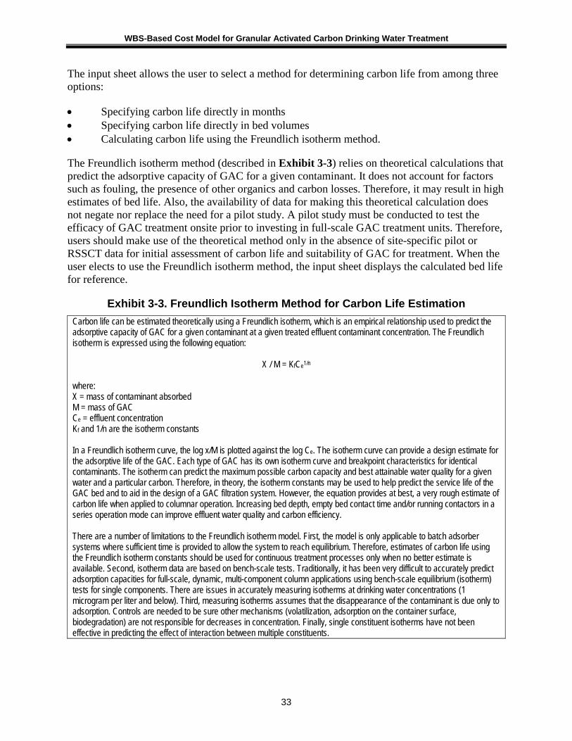
WBS-Based Cost Model for Granular Activated Carbon Drinking Water Treatment
33
The input sheet allows the user to select a method for determining carbon life from among three options:
• Specifying carbon life directly in months • Specifying carbon life directly in bed volumes • Calculating carbon life using the Freundlich isotherm method.
The Freundlich isotherm method (described in Exhibit 3-3) relies on theoretical calculations that predict the adsorptive capacity of GAC for a given contaminant. It does not account for factors such as fouling, the presence of other organics and carbon losses. Therefore, it may result in high estimates of bed life. Also, the availability of data for making this theoretical calculation does not negate nor replace the need for a pilot study. A pilot study must be conducted to test the efficacy of GAC treatment onsite prior to investing in full-scale GAC treatment units. Therefore, users should make use of the theoretical method only in the absence of site-specific pilot or RSSCT data for initial assessment of carbon life and suitability of GAC for treatment. When the user elects to use the Freundlich isotherm method, the input sheet displays the calculated bed life for reference.
Exhibit 3-3. Freundlich Isotherm Method for Carbon Life Estimation Carbon life can be estimated theoretically using a Freundlich isotherm, which is an empirical relationship used to predict the adsorptive capacity of GAC for a given contaminant at a given treated effluent contaminant concentration. The Freundlich isotherm is expressed using the following equation:
X / M = KfCe1/n
where: X = mass of contaminant absorbed M = mass of GAC Ce = effluent concentration Kf and 1/n are the isotherm constants In a Freundlich isotherm curve, the log x/M is plotted against the log Ce. The isotherm curve can provide a design estimate for the adsorptive life of the GAC. Each type of GAC has its own isotherm curve and breakpoint characteristics for identical contaminants. The isotherm can predict the maximum possible carbon capacity and best attainable water quality for a given water and a particular carbon. Therefore, in theory, the isotherm constants may be used to help predict the service life of the GAC bed and to aid in the design of a GAC filtration system. However, the equation provides at best, a very rough estimate of carbon life when applied to columnar operation. Increasing bed depth, empty bed contact time and/or running contactors in a series operation mode can improve effluent water quality and carbon efficiency. There are a number of limitations to the Freundlich isotherm model. First, the model is only applicable to batch adsorber systems where sufficient time is provided to allow the system to reach equilibrium. Therefore, estimates of carbon life using the Freundlich isotherm constants should be used for continuous treatment processes only when no better estimate is available. Second, isotherm data are based on bench-scale tests. Traditionally, it has been very difficult to accurately predict adsorption capacities for full-scale, dynamic, multi-component column applications using bench-scale equilibrium (isotherm) tests for single components. There are issues in accurately measuring isotherms at drinking water concentrations (1 microgram per liter and below). Third, measuring isotherms assumes that the disappearance of the contaminant is due only to adsorption. Controls are needed to be sure other mechanisms (volatilization, adsorption on the container surface, biodegradation) are not responsible for decreases in concentration. Finally, single constituent isotherms have not been effective in predicting the effect of interaction between multiple constituents.

WBS-Based Cost Model for Granular Activated Carbon Drinking Water Treatment
34
Carbon life for atrazine removal calculated using the Freundlich isotherm method is on the order of a few hundred months. Actual carbon life has proven to be much shorter in pilot- and full-scale implementation. Therefore, the model standard designs assume a carbon life of 12 months for atrazine removal to be conservative and account for the factors noted above. Standard designs for radon assume a carbon life of 24 months (2 years), given that a GAC bed used for radon removal can last for many years, assuming no limiting water quality conditions exist. Standard design assumptions for VOCs are under development; values used in the model are based on preliminary results from EPA pilot tests.
Contaminant Removal Requirements For a given set of site-specific conditions, there is a minimum empty-bed contact time (EBCT) required to produce water of acceptable quality. EBCT is defined by the following equation:
EBCT = Bed Volume/Volumetric Flow Rate Because the minimum EBCT required varies depending on the specific contaminant treated, the required contaminant removal percentage, the type of GAC used and other influent water characteristics (e.g., the presence of competing chemical species), EBCT is best determined using pilot studies or previous experience with GAC systems for similar influent waters.
For radon, however, EBCT can be determined theoretically. This is because, in theory, a steady state condition develops in the bed in which the rate of radon adsorption equals the radioactive decay of adsorbed radon. Thus, adsorption of radon can be modeled using the equation shown in Exhibit 3-4.
Exhibit 3-4. Modeling Radon Adsorption Adsorption of radon can be modeled using the equation:
Ce/C0 = e-Kss*EBCT where: Ce = effluent concentration C0 = influent concentration Kss = steady state rate coefficient (in hours-1) EBCT = empty bed contact time (in hours) Thus, if Ce, C0 and Kss are known, the required EBCT can be calculated as:
EBCT = Ln[ (C0/Ce) * Kss ] The input sheet requires the user to select a method for determining EBCT either by specifying EBCT directly (the preferred method) or calculating it by entering contaminant concentrations (or percent removal) and Kss. This latter method should be used only for radon. Reported values for Kss for radon range from 1.3 to 5.7 hours-1 (Drago, 2000). For reference, when the user elects to use a Kss to calculate EBCT for radon, the input sheet displays the resulting EBCT. Typical EBCT values are between 5 and 25 minutes for organic chemicals (AWWA/ASCE, 1998), while typical EBCTs for radon are much higher. The model standard designs for atrazine use an EBCT

WBS-Based Cost Model for Granular Activated Carbon Drinking Water Treatment
35
of 15 minutes, based on the recommendations of peer reviewers. The standard designs for radon use an EBCT of 30 minutes, consistent with 75 percent removal and a Kss of 3 hours-1.
Number of Contactors in Series (Parallel or Series Operation) For pressure GAC trains with high EBCT values (e.g., greater than 10 minutes), a treatment train consisting of a number of vessels in series can be effective. The use of multiple vessels in a series (or lead/lag) can extend overall bed life compared to a single vessel with a similar total bed volume. Initial vessels in the series serve as roughing vessels and subsequent vessels are polishing vessels. When GAC in the roughing vessel is spent, this media is replaced and the polishing vessel moves to the start of the series, becoming the roughing vessel. The use of vessels in series also can allow the carbon in the lead vessel to reach saturation and can increase total capacity by about 10 to 30 percent (Calgon, 1999). Because of the high EBCT required for atrazine and radon (15 to 30 minutes), the model standard designs assume three vessels in series when pressure GAC designs are selected for these contaminants. Gravity GAC systems typically are operated with contactors in parallel, rather than series. Therefore, when gravity designs are selected, the GAC model designs systems with contactors in parallel and disables this input.
Bed Depth and Contactor Dimensions For both design types (pressure and gravity), the input sheet requires the user to input the desired depth of the GAC bed. For gravity contactors, typical bed depths are between 3 and 10 feet. For pressure contactors, typical bed depths are between 2 and 8.5 feet. For preliminary design, other sources of a reasonable bed depth include the designer’s past experience, manufacturer recommended bed depth and published literature. The model standard designs use bed depths meeting these constraints. The specific input fields for contactor dimensions other than bed depth differ between the two design types, as described below. For both design types, the model includes a computer-aided design routine, also described below, to assist users in selecting dimensions.
Pressure Vessel Dimensions and Geometry For pressure GAC designs, the input sheet requires the user to select vessel geometry. Options are vertical vessels for small to medium sized systems and horizontally laid long vessels for large systems. For either configuration, the user needs to input the straight height or length of the vessel and the diameter of the vessel. Pressure vessels used in this application typically are upright cylinders, with a diameter ranging from 1.5 to 14 feet and up to 14 feet in height. Very large systems (e.g., with design flows greater than 2,000 gallons per minute [gpm]) can use horizontally laid vessels 20 to 40 feet long and up to 14 feet in diameter.
The input sheet will display warning signs if the dimensions of the selected vessel are outside the boundaries specified on the critical design assumptions sheet. These boundaries include loading rates, which are discussed in more detail in Section 3.3, and transportation limitations. For large treatment plants, on-site assembly of tanks might be an option to overcome transportation limitations. To allow this option, the user should increase the maximum dimensions permitted on the critical design assumptions sheet.

WBS-Based Cost Model for Granular Activated Carbon Drinking Water Treatment
36
Gravity Contact Basin Dimensions For gravity GAC designs, the input sheet requires the user to input the desired width and length of the GAC contact basins. GAC contact basins typically are square. The input sheet will display warning signs if the dimensions of the selected basin are outside the boundaries specified on the critical design assumptions sheet. These include loading rates, which are discussed in more detail in Section 3.3, and reasonable size limitations based on generally recommended engineering practices (GREPs). The size limitations (which can be modified by the user on the critical design assumptions sheet) are:
• GAC bed depth of 3 to 10 feet • Width and length of 6 to 30 feet.
Autosize Routine To aid users, the model includes buttons labeled “Autosize” for each design type (pressure or gravity). These buttons activate a computer-aided design routine that attempts to find a design that meets all relevant design constraints for a given design and average flow and minimizes annualized cost. Using the autosize routine, the model will automatically select bed depth, geometry and dimensions that meet all constraints, thus reducing trial and error by users, particularly for systems with design flows other than the eight standard sizes provided on the input sheet. Note that all other inputs must be complete before using the autosize routine.
Interval between Backwashes Like conventional filters, GAC contactors must be backwashed periodically to remove solids, maintain the desired hydraulic properties of the bed and possibly to control biological growth. The physical properties of GAC particles affect filtration and backwash properties. These physical properties include particle hardness, size and bed uniformity. Generally, a large uniformity coefficient is recommended to maintain hydraulic and contaminant removal uniformity. Particle density and size also affect backwashing. Generally, the harder the particle, the less attrition of GAC during backwashing. The interval between backwash occurrences is a function of the turbidity in the water and is typically 24 to 72 hours, although the interval can be even longer for post-filter applications of GAC. For example, based on peer reviewer comments, unfiltered surface water will require backwash every 24 to 48 hours while filtered surface water will require backwash every 14 to 30 days. The typical backwash interval for groundwater can be 7 days or more. The input sheet requires the user to enter the interval (in hours) between backwash events. The model standard designs use 48 hours between backwashes for atrazine, consistent with unfiltered surface water and 168 hours (7 days) for radon and various VOCs, consistent with groundwater. Users wishing to model treatment of these contaminants in different quality water (e.g., atrazine in groundwater or filtered surface water) should adjust the backwash interval.
GAC Transfer Method Transfer equipment is needed to remove spent GAC from the contactors and fill the contactors with regenerated or replacement GAC. The transfer of the media to and from the contactors can be accomplished manually or mechanically using eductors. The GAC model does not consider the use of slurry pumps because this method could result in excessive attrition of the media. The input sheet requires the user to select the transfer method. The model standard designs select

WBS-Based Cost Model for Granular Activated Carbon Drinking Water Treatment
37
manual transfer for systems for which this option resulted in relatively low labor requirements (i.e., those requiring infrequent removal of small quantities of media). The standard designs use eductors for all other systems.
Residuals Management GAC systems generate two residuals streams on an intermittent basis: spent backwash and spent media. The input sheet requires the user to choose from among several options for management of each of these residuals streams. Exhibit 3-5 shows the management options available for spent backwash.
Exhibit 3-5. Management Options for Spent Backwash Options for Stage 1 of Management Options for Stage 2 of Management
Holding tank with or without coagulant addition (for flow equalization and suspended solids removal)*
Direct discharge to surface water Discharge to POTW Recycle to head of treatment train
No holding tank Direct discharge to surface water Discharge to POTW Septic system* Evaporation pond*
* Results in generation of secondary residuals (holding tank settled solids, septic tank solids or evaporation pond solids). The management options shown in Exhibit 3-5 include the option for a holding tank. The purpose of the holding tank is to equalize the rate of flow at which residuals are released or discharged. When averaged over the time between generation events, backwash flow is relatively low. However, instantaneous flow during a generation event is much higher. If spent backwash is recycled to the head of a treatment plant, recommended engineering practice is that the recycle stream should be no more than 5 to 10 percent of total system flow (U.S. EPA, 2002; U.S. EPA, 1996). Given the instantaneous backwash flow rates, if recycling is chosen for stage 2 of management, a holding tank would always be necessary to prevent recycle flow from exceeding this recommendation. It also may be reasonable to include a holding tank for the other stage 2 options (e.g., to prevent instantaneous flow from overwhelming the capacity of a publicly owned treatment works [POTW]).
The use of a holding tank can result in the generation of a secondary residuals stream, in the form of solids that settle from the spent backwash during the holding period. When a holding tank is used, the model includes the option to add a coagulant to promote the settling of these solids and reduce suspended solids levels in the holding tank effluent. As a default, the model assumes coagulant addition is not utilized. The user can change this option on the critical design assumptions sheet.
Exhibit 3-5 also includes the option for an evaporation pond. Given the quantities of spent backwash generated, use of this management method is unlikely, but might be considered for facilities in very dry climates. The required area for an evaporation pond depends on local climate. After selecting an evaporation pond, the user should carefully review the climatic parameters on the critical design assumptions sheet. For more information, see Appendix C. Furthermore, to ensure that heating, cooling and standby power costs are computed consistently,

WBS-Based Cost Model for Granular Activated Carbon Drinking Water Treatment
38
the user should review the climatic parameters in the operating and maintenance (O&M) and indirect assumptions sheets. Appendix E and Appendix D contain information on these parameters. The use of an evaporation pond results in the generation of a secondary residuals stream, in the form of evaporation pond solids.
A holding tank would not be required with an evaporation pond, because the design of the pond would provide sufficient capacity to handle instantaneous flow. A holding tank also would not be required with a septic system, since the septic tank itself serves as a holding tank.
Carbon regeneration or replacement is necessary when the adsorption capacity is used up and contaminant breakthrough has occurred. The regeneration process has four basic steps: drying, vaporization, pyrolysis and oxidation of the pyrolized residue (char). Common methods include multiple hearth, rotary kiln, fluidized bed furnace and infrared furnace. Some systems have the ability to regenerate GAC onsite, but most small systems haul away the spent GAC for off-site regeneration (U.S. EPA, 1993) or disposal in a non-hazardous solid waste landfill. The input sheet, therefore, requires the user to select from among the following seven options for handling spent GAC:
1. On-site regeneration 2. Off-site regeneration 3. Off-site regeneration when spent GAC would be classified as hazardous waste 4. Disposal as non-hazardous solid waste 5. Disposal as hazardous waste 6. Disposal as radioactive waste 7. Disposal as radioactive and hazardous waste.
Management options available for secondary solid residuals (e.g., holding tank solids) include the four disposal methods (i.e., options 4 through 7 above).6
The model does not include on-site regeneration of spent media that would be classified as hazardous, because this option would likely entail excessive costs associated with permitting the treatment unit. When on-site regeneration is selected (option 1 above), the system will include on-site regeneration capacity using a multiple hearth furnace and on-site facilities (tanks or basins) for GAC storage before and after regeneration. The disposal options (options 4 through 7 above) for spent GAC are present for situations where the media is used on a throwaway basis without regeneration. For both secondary residuals and spent GAC, the disposal options (options 4 through 7 above) assume disposal in an off-site facility.7
For spent backwash, the model standard designs assume the use of a holding tank for systems generating residual flow rates greater than 100 gpm during backwash. The standard designs assume discharge to a POTW for the second stage of spent backwash management. For spent 6 Users can also select land application, instead of landfilling, for non-hazardous secondary residuals by changing an option on the critical design assumptions sheet. Appendix C discusses this option in more detail. 7 The management options do not include disposal in an on-site facility. This option would be economically viable only for facilities with an existing on-site landfill—a factor that is highly site-specific. For these facilities, the cost of this option would be less than that for off-site disposal, because it would involve much lower transportation costs. Therefore, the off-site disposal options included provide a conservative cost estimate for these facilities.

WBS-Based Cost Model for Granular Activated Carbon Drinking Water Treatment
39
GAC for atrazine, the standard designs assume off-site regeneration for all but the smallest system size. For the smallest system size for atrazine, the standard designs assume throwaway operation using an off-site non-hazardous waste landfill. For radon, the standard designs assume throwaway operation using an off-site radioactive waste facility for all system sizes, because of concerns about the feasibility of regenerating carbon used for radionuclides removal. For systems that generate holding tank solids, the standard designs assume non-hazardous waste landfill disposal for this residuals stream.
Number of Booster Pumps Review of actual as-built designs for small systems using various technologies (U.S. EPA, 2004) shows that these systems often can operate without additional booster pumps using existing supply pump pressure. Therefore, the model assumes zero booster pumps for small systems (less than 1 MGD design flow). For larger systems, the model calculates the number of pumps using a method that attempts to minimize the number of pumps, while still accommodating variations in flow and providing redundancy to account for possible equipment failure. The model includes an optional input that allows the user to change these default calculations by specifying the number of pumps required to operate the treatment system. If the user enters zero, the model excludes booster pumps from the design and cost estimate. The standard designs for atrazine leave this input blank, excluding booster pumps for small systems and accepting the default calculations for larger systems. The standard designs for radon exclude booster pumps for all sizes of pressure GAC systems, because the designs assume the treatment of groundwater with sufficient existing supply pump pressure. They leave the input blank for gravity GAC systems, thereby including booster pumps for large systems (1 MGD or greater design flow).
Number of Redundant Contactors This optional input controls the model’s calculation for the number of redundant contactors. At a minimum, based on the Technology Design Panel recommendations, there should be at least one redundant contactor in a GAC treatment system. An exception would be small pressure systems designed with multiple contactors required to treat the maximum design flow (either more than one parallel treatment train or a single line with multiple contactors in series). In such systems, the average daily flow is low enough, relative to the design flow, that the multiple contactor design provides sufficient redundancy without additional vessels. The system can operate at reduced, but greater than average, flow, even while one contactor is off-line for backwashing or GAC replacement. Thus, the number of redundant contactors can be zero for certain small systems having at least two vessels.
The model assumes that redundant contactors (and other redundant items of equipment) are used during downtime periods for other contactors and swapped into operation intermittently, with other contactors then becoming standby. For this reason, the O&M estimate in the model includes labor for operating valves and reading instruments associated with redundant contactors.
The input sheet allows the user to specify the number of redundant contactors. If the user leaves this optional input blank for a large pressure GAC system (1 MGD or greater design flow) or any gravity GAC system, the model calculates the number of redundant contactors based on a redundancy frequency specified on the critical design assumptions sheet. If the user leaves this optional input blank for a small pressure GAC system (less than 1 MGD design flow), the model

WBS-Based Cost Model for Granular Activated Carbon Drinking Water Treatment
40
does not add redundant contactors, unless the design selected by the user results in a single operational contactor. In this latter scenario, the model adds one redundant contactor.
The standard designs leave this input blank, resulting in the following redundancy results:
• No redundant contactors for small systems (less than 1 MGD design flow), except in cases where the design results in only one operating filter
• One redundant contactor every four treatment trains for larger pressure systems (1 MGD or greater design flow)
• One redundant contactor total for medium gravity systems (1 MGD to less than 10 MGD design flow) gravity systems
• Two redundant contactors total for larger gravity systems (10 MGD or greater design flow).
Backwash Pumping The backwash process can require new pumps or use existing pumps (either influent supply pumps or treated water pumps, assuming these pumps can deliver unchlorinated treated water). The practicality of using existing pumps can vary on a site-specific basis, depending on the performance characteristics of the existing pumps and the differences in head required between normal operation and during backwash. By default, the model assumes existing pumps are sufficient for backwash for small systems (less than 1 MGD design flow), but includes the costs of new backwash pumps for larger systems. The model includes an optional input that allows the user to change these default assumptions by explicitly selecting “existing pumps” or “new pumps.” If the “existing pumps” option is selected, the costs of backwash pumps will be excluded from the output sheet. If “new pumps” is selected, these costs will be included. The standard designs leave this input blank, thereby assuming the use of existing pumps for small systems (less than 1 MGD design flow), but including the costs of backwash pumps for larger systems.
Backwash Storage Backwash tanks may not be required on most installations, particularly for large systems that have treated water storage capacity. The model assumes that systems with design flow less than 1 MGD do not require backwash tanks because the quantity of backwash water required is low. The model also assumes that systems of 10 MGD and larger design flow do not require backwash tanks because existing storage capacity is sufficient. The model includes backwash tanks for intermediate-sized systems. The model includes an optional input that allows the user to change these default assumptions by explicitly selecting “existing storage” or “new storage.” If the “existing storage” option is selected, the costs of backwash tanks will be excluded from the output sheet. If “new storage” is selected, these costs will be included. The standard designs leave this input blank, thereby including the costs of backwash tanks for intermediate-sized systems (1 MGD to less than 10 MGD design flow) only.
Add-On (Pre- or Post-Treatment) The WBS model for GAC includes an optional input that allows the user to specify that the GAC treatment system is an addition to an existing treatment plant, intended as pre- or post-treatment

WBS-Based Cost Model for Granular Activated Carbon Drinking Water Treatment
41
for another primary treatment process.8 When the user selects “add-on” for this input, the model changes certain assumptions and calculations to reflect this scenario. Specifically, the model excludes (or reduces the quantity or size of) certain capital components that would already be present at the existing treatment plant. For example, the model includes only the incremental system control components that would be required to integrate with the existing treatment process control system. It includes O&M cost items because the model calculates them on an incremental basis (e.g., the labor hours cover only the additional hours required to operate the new GAC process).
In the “add-on” scenario, the model also excludes certain indirect costs that would be required in constructing a full new treatment plant. Specifically, the model does not include yard piping, because installing the add-on process should not require additional exterior pipelines. It also does not include standby power costs, because the additional electrical demand from the add-on process should not require significant additional standby capacity. Add-on systems using pressure GAC exclude geotechnical costs, because the pre-existing geotechnical survey for the treatment plant should be sufficient to cover the construction associated with the add-on process. However, add-on systems using gravity GAC include geotechnical costs because additional surveying may be needed for excavation of the contact basins.
Finally, although the GAC process is assumed to be an addition to an existing treatment plant in the add-on scenario, the model does include the full cost of buildings and land for the incremental footprint of the process. While some treatment plants might be able to accommodate the new process within existing space, others will require expansion to house the process. Therefore, the inclusion of buildings and land is conservative (i.e., errs on the side of higher costs) in terms of the actual cost of installing the process. Furthermore, even where existing buildings and land are sufficient, the use of this existing space represents an economic opportunity cost that is appropriate to include in regulatory cost estimates.
Retrofit (Operational Modification) When faced with changing regulatory requirements (e.g., lower concentration limits) or new contaminants in the water supply, existing GAC treatment plants can sometimes achieve additional removal by increasing carbon regeneration or replacement frequency so that the removal capacity of the media is restored before breakthrough at a new, lower target concentration (or breakthrough of the new contaminant). In other words, the GAC treatment system achieves the additional removal by modifying operations to reflect a new, shorter carbon life.
The WBS model for GAC includes an optional input that directs the model to estimate costs for this type of operational modification. When the user selects “retrofit” for this input, the model also requires the user to provide input for the new, shorter carbon life. The input options for the post-modification carbon life are identical to those for the original carbon life described above. After the user enters the new carbon life, the model estimates the incremental costs associated
8 The current model includes a set of standard designs that use the add-on optional input to model the use of GAC for post-treatment to quench hydrogen peroxide for UV-AOP. These standard designs should only be used in conjunction with the UVAOP model, which is under development. Standard designs for other contaminants leave the add-on optional input blank.

WBS-Based Cost Model for Granular Activated Carbon Drinking Water Treatment
42
with the operational modification. Except when on-site regeneration is selected, these costs are limited to incremental O&M costs (e.g., GAC media costs and incremental labor costs associated with more frequent regeneration or replacement). When on-site regeneration is selected, the model also includes capital costs associated with expanding the multiple hearth furnace to provide additional regeneration capacity. The model standard designs do not consider operational modifications and leave this input blank.
Model Assumptions Sheets 3.3There are three sheets that contain assumptions needed to facilitate process design: the critical design assumptions sheet, the O&M assumptions sheet and the indirect assumptions sheet. These sheets contain a variety of structural and chemical engineering parameters used in the engineering design sheets. They also interact with the input sheet to determine if the user inputs violate good engineering practices. For example, if a user selects contactor dimensions that generate a surface loading rate that is too high or low, a warning message will appear on the input sheet. The warning message will advise the user to adjust contactor dimensions or bed depth to achieve a surface loading rate within GREPs.
There are more than 100 critical design assumptions in the model that cover process, O&M and indirect cost parameters. Key critical design assumptions include surface loading rate, bed expansion, backwash assumptions, regeneration and transfer assumptions, bypass percentage and assumptions applicable to package plants. The following sections provide descriptions and default values for these assumptions. Any assumption value can be modified, as needed.
Surface Loading Rate A loading rate is the velocity of flow through the media measured in units of flow rate per unit area (e.g., gallons per minute per square foot [gpm/ft2]). The surface area of the contactors must be selected to maintain loading rates within reasonable bounds because water can channel through the carbon bed if the loading rate is too low and pressure requirements may be excessive if the loading rate is too high. For GAC treatment systems, loading rates usually are between 2 gpm/ft2 and 10 gpm/ft2. Higher loading rates may be used in site-specific situations where hydraulics and tests allow. The model assumes a maximum loading rate of 10 gpm/ft2 and a minimum loading rate of 0.5 gpm/ft2.
Bed Expansion Vessel height (in pressure GAC designs) or contact basin depth (in gravity GAC designs) must account for bed expansion during backwash. Gravity contactors also must provide freeboard to prevent media washout. Bed expansion values should be taken from media vendor catalogues and verified in pilot studies. Typical bed expansion generally is at least 50 percent (AWWA/ASCE, 1998). The model assumes bed expansion of 50 percent and gravity designs add 2 feet of freeboard above bed expansion.
Backwash Assumptions Backwash rates appropriate for specific GACs are provided by the manufacturer. Backwash rates should be sufficient to fluidize the bed and should allow for the expansion of the GAC media during backwash (AWWA/ASCE, 1998). The model assumes a backwash rate of 12 gpm/ft2 and a backwash duration of 10 minutes.

WBS-Based Cost Model for Granular Activated Carbon Drinking Water Treatment
43
Regeneration and Transfer Assumptions When the user selects regeneration (either on-site or off-site), a key assumption relates to GAC losses during regeneration and transfer. The model expresses this assumption as the GAC makeup rate, because it is used to calculate the quantity of virgin GAC required per year to replace these losses. For on-site regeneration, the model assumes a GAC makeup rate of 10 percent per year. Makeup carbon needs are higher for off-site transportation and regeneration, so the model assumes a makeup rate of 30 percent per year.
For on-site regeneration, a number of additional key assumptions are needed to size the regeneration and storage facilities. These assumptions are regeneration facility run time, regeneration facility redundancy and GAC storage facility capacity. Section 3.5 below, describing the backwash and regeneration sheet, discusses the use of these assumptions.
Bypass Percentage Systems may choose to treat only a portion of their production flow, using a smaller treatment system and blending treated water with raw water while still achieving treatment targets. The bypass percentage is that portion of production flow that goes untreated. If bypass is used, the model designs the treatment system to treat a flow equal to (100 minus bypass percentage) multiplied by design flow and adds bypass piping and associated valves to the components included on the output sheet. The model assumes no bypass, but the user can incorporate bypass by entering a percentage of bypass flow on the critical design assumptions sheet.
Package Systems The GAC model handles package systems by costing all individual equipment line items (e.g., vessels, interconnecting piping and valves, instrumentation and system controls) in the same manner as custom-engineered systems. This approach is based on vendor practices of partially engineering these types of package plants for specific systems (e.g., selecting vessel size to meet flow and treatment criteria). For small systems (less than 1 MGD design flow), the model applies a variant set of design inputs and assumptions that are intended to simulate the use of a package plant. Also included are assumptions that reflect the smaller capacity and reduced complexity of the treatment systems. These design modifications typically reduce the size and cost of the treatment system. Some are adjustable on the input sheet or the critical design assumptions sheet, while others are in the engineering design formulae. Exhibit 3-6 shows the design modifications used in the GAC model for small systems.
Exhibit 3-6. Variant Design Inputs and Assumptions for Small Systems Small System Design
Modification Explanation Model Location
Reduced spacing between vessels and other equipment
This assumption simulates skid placement of treatment vessels (and of pumps, if included in the design), resulting in reduced system footprint and, therefore, reduced costs for interconnecting piping, building structures, certain indirect costs and O&M.
Design equations on the pumps, pipes and structure sheet
No redundant vessels (but a minimum of two operating vessels)
Small systems typically do not include redundant treatment vessels because they are designed to operate at reduced capacity during the brief periods when one vessel is not operating (e.g., during backwash).
Input sheet

WBS-Based Cost Model for Granular Activated Carbon Drinking Water Treatment
44
Small System Design Modification Explanation Model Location
Reduced instrumentation requirements
Instrumentation required for small systems is limited to flow meters, high/low alarms, turbidity meters (in gravity systems) and sampling ports.
Critical design assumptions sheet
Simplified system controls for automated systems
Package plants, when automated, typically are controlled by a single, pre-programmed operator interface unit mounted on the skid. Therefore, for small systems, the model uses this type of operator interface only and excludes the multiple programmable logic controllers, computer workstations, printers, operator interface software and plant intelligence software included for large, automated, custom-engineered systems.
Component selection logic in the output sheet and WBS cost database
No booster pumps Small GAC systems result in limited head loss and typically do not require additional booster pumps.
Input sheet
No backwash pumps or tanks
Small systems typically use existing pumps and water supplies and do not require separate backwash pumps or backwash water storage.
Input sheet
Reduced concrete pad thickness
Small capacity systems require less structural support. Critical design assumptions sheet
Reduced indirect costs Package plants require less effort to design and install. Therefore, the model reduces or eliminates certain indirect costs (e.g., mobilization/demobilization, construction management) for small package plants (see Appendix D for complete details).
Indirect assumptions sheet
Contactor Constraints Sheet 3.4
The contactor constraints sheet contains calculations that utilize the user-defined parameters from the input sheet and the boundary values from the critical design assumption sheet to determine the validity of the input values. This sheet also determines the number of contactors required and the quantity of GAC needed, given the input values selected by the user. For gravity GAC designs, this sheet also calculates the total volume of concrete required and, because contact basins are constructed below grade, determines excavation and backfill requirements.
Backwash and Regeneration Sheet 3.5The backwash and regeneration sheet calculates the total backwash volume required to backwash one contactor, based on the contactor surface area, backwash loading rate and backwash time. The sheet uses this value to calculate backwash storage requirements. Water for backwash can be stored in steel, fiberglass or plastic backwash tanks. This sheet calculates the total volume of each tank. Because it is appropriate for larger systems, this sheet also considers the use of concrete basins for backwash storage. For concrete basins, the model assumes one basin and calculates length, width and depth based on standard dimensional ratio assumptions. The user can change these assumptions on the critical design assumptions sheet. Based on these dimensions, the model then calculates the total volume of concrete required, along with excavation and backfill requirements.
This sheet also calculates the GAC bed life using the method specified on the input sheet (directly specified in months or bed volumes or calculated using the Freundlich Isotherm method). Based on this bed life and the quantity of GAC calculated on the contactor design sheet, this sheet then calculates the annual GAC regeneration or replacement needs.

WBS-Based Cost Model for Granular Activated Carbon Drinking Water Treatment
45
For systems using on-site regeneration, the sheet calculates the design capacity of the regeneration facility (multiple hearth furnace) and the GAC storage requirements. To determine regeneration facility capacity, the sheet first calculates average daily regeneration required in pounds of GAC per day, based on the total quantity of GAC for all contactors and the bed life. The sheet then calculates design regeneration capacity using the following equation:
D = (A / Run time) x Redundancy
where:
D is design regeneration facility capacity in pounds per day A is average daily regeneration rate in pounds per day Run time is the regeneration facility run time as a percentage of full time operation as specified on the critical design assumptions sheet (the default assumption is 85 percent to account for routine maintenance) Redundancy is an additional safety factor expressed as a percentage greater than or equal to 100 percent and specified on the critical design assumptions sheet (the default assumption is 100 percent, providing no additional capacity beyond that needed to account for downtime during maintenance).
The sheet calculates GAC storage requirements for spent GAC (i.e., awaiting regeneration), regenerated GAC (i.e., awaiting use) and virgin GAC (i.e., makeup GAC to replace losses). The quantity of each type of GAC stored is equal to the GAC capacity of a single contactor multiplied by a factor specified on the critical design assumptions sheet. The default capacity factor for each of spent, regenerated and virgin GAC is 1.33. GAC storage for each can be steel tanks or concrete basins and the sheet calculates the size of these storage facilities using the same approach as for backwash tanks and basins.
Retrofit Sheet 3.6When the “Retrofit (operational modification)” input is set to “retrofit” on the input sheet, the retrofit sheet performs the calculations required to estimate the cost associated with operational modifications to use a new, shorter carbon life. This sheet duplicates the bed life and regeneration calculations on the backwash and regeneration sheet using the new carbon life in place of the original carbon life. It then compares the results to those on the backwash and regeneration sheet to calculate the incremental GAC usage associated with the operational modification. This sheet also calculates the other incremental requirements associated with the operational modification, such as operator labor, energy use and regeneration furnace capacity (if required).
Pumps, Pipe and Structure Sheet 3.7Other elements of the technology for which the size and cost need to be determined include pumps, piping and GAC transfer equipment (eductors). The pumps, pipe and structure sheet performs the required calculations to determine the number and size (in terms of flow capacity) of the following pumps:
• Booster pumps • Backwash pumps (if required).

WBS-Based Cost Model for Granular Activated Carbon Drinking Water Treatment
46
This sheet uses the input values for flow and water quality parameters, as well as the pertinent parameters detailed on the critical design assumption sheet, to determine the number of pumps needed, including redundant units. Pump sizing depends on the maximum corresponding flow rate. For example, booster pumps are sized based on the system design flow and backwash pumps are sized based on the total backwash flow. As discussed in Section 2.3, the sizing of all pumps incorporates a safety factor, which is specified on the critical design assumptions sheet.
This sheet also performs calculations for the following pipes:
• Influent and effluent piping • Process piping • Backwash piping • Bypass piping (if a bypass percentage is specified).
The size (diameter) of pipes is determined using a pipe flow lookup table. The pipe diameter selection method incorporates a reasonable head loss and flow velocity, as documented in Exhibit 2-8. These design assumptions may result in some over sizing of pipes and, therefore, the resulting cost estimates may be conservative (i.e., err on the high side).
The flow used to determine influent and effluent pipe size is the design flow. The diameter of interconnecting process piping uses the same pipe flow chart, after splitting the inflow by the number of parallel treatment trains. A similar approach is used in determining the size and capacity of backwash and bypass piping. The length of these pipes is determined using the assumptions documented in Exhibit 2-10, which are designed to account for the cost of fittings.
This sheet also calculates the housing area for this technology based on the footprint of the technology components and the spacing criteria specified on the critical design assumption sheet. The space requirements for contactors, pumps, tanks and service space are based on manufacturer specification, “to scale” drawings and the experience of engineers. The amount of additional concrete needed to support heavy equipment, such as pumps and pressure contactors, is based on the footprint of the contactors and pumps.
For smaller space requirements (less than a square footage specified on the critical design assumptions sheet), the model assumes a single building containing all process equipment. For larger requirements, the model assumes two buildings, one containing the GAC contactors and the other containing all other equipment. The number of buildings affects the total land required and energy costs for heating, ventilating and cooling.
Instrumentation and Control Sheet 3.8The instrumentation and control sheet calculates requirements for valves, instrumentation (e.g., flow meters) and automated system controls. The number of valves and instruments is based on the number of process components (e.g., number of treatment lines) and assumptions from the critical design assumptions sheet (e.g., x number of valves per treatment line). The assumptions correspond to the general schematic layout for this technology shown in Exhibit 3-1 and Exhibit 3-2. Sizing of valves corresponds to the size of the appropriate pipe determined on the pumps, pipes and structure sheet. Appendix A describes the method used in the WBS models to estimate the number and type of system control components.

WBS-Based Cost Model for Granular Activated Carbon Drinking Water Treatment
47
Residuals Management Sheet 3.9The residuals management sheet estimates the volume and mass of residuals, their characteristics and the capital and O&M requirements for residuals management, based on the management options selected on the input sheet and the approach outlined in Appendix C. Depending on the management options chosen, specific items of capital equipment for residuals can include:
• Holding tanks • Pumps • Septic tanks and drain field components • Evaporation ponds (including excavation and lining) • Coagulant feed and mixing equipment • Valves, piping and instrumentation.
Specific O&M requirements associated with residuals can include:
• Residuals pump labor, materials and energy • POTW discharge fees • Coagulant usage • Spent GAC transportation and disposal costs • Secondary residuals (holding tank or septic tank solids) transportation and disposal costs.
O&M and HVAC Sheets 3.10The O&M and heating, ventilating and air conditioning (HVAC) calculations cover two sheets: the O&M sheet (annual labor, materials and energy usage) and the HVAC sheet (HVAC capacity requirements). The O&M sheet derives annual O&M requirements for GAC treatment based on the engineering design, O&M critical design assumptions and input values. It determines the following O&M requirements based on the approach outlined in Section 2.4 and Appendix E:
• Operator labor for system operation and maintenance • Managerial and clerical labor • Booster pump maintenance materials and operating energy • Facility maintenance materials • Energy for building lighting and HVAC.
In addition, the O&M sheet adds the following technology-specific O&M requirements:
• Operating energy for backwash pumps • Operator labor and materials for backwash pump maintenance (if backwash occurs
weekly or more frequently) • Operator labor for managing backwash events • Operator labor for media transfer • Operator labor for contactor maintenance (for gravity GAC designs)

WBS-Based Cost Model for Granular Activated Carbon Drinking Water Treatment
48
• Materials for contactor maintenance (accounts for vessel relining in pressure designs, because GAC can be corrosive and for concrete and underdrain maintenance in gravity designs)
• Labor, materials, energy and natural gas usage for on-site GAC regeneration (if this option is chosen by the user).
Because GAC systems are backwashed frequently, backwash pumping facilities consume more energy than in other technologies and can require significant maintenance. Therefore, the model includes backwash pump operating energy among its O&M costs. When backwash occurs weekly or more frequently, the model also explicitly includes labor and materials for maintaining backwash equipment. The sheet determines materials for backwash pumps using the same approach outlined in Appendix E for booster or influent pumps. Backwash pump labor uses the equation described in Appendix E for booster or influent pumps, except that the maximum total backwash flow is substituted for system design flow. Backwash pump energy consumption also follows the approach in Appendix E, except that, rather than assuming continuous operation, the calculation uses the number of hours per year during which backwash pumps operate.
For manual and semi-automated systems, backwashing requires constant operator attention. Therefore, the model assumes labor equal to twice the actual time to accomplish backwash for these systems. For automated systems, the model assumes 1 minute per backwash event to verify that the automated backwash cycle is initiated and operating properly. The user can change this latter assumption on the O&M assumptions sheet.
The model also assumes the annual cost of materials for contactors is equal to 1 percent of their pre-installation capital cost. For gravity GAC designs, the O&M sheet determines labor for basin maintenance assuming 1 hour per week for each contact basin. The user can change these assumptions on the O&M assumptions sheet.
The O&M sheet determines labor, materials and energy requirements for on-site regeneration using equations derived in U.S. EPA (2000) and presented in Exhibit 3-7.
Exhibit 3-7. O&M Equations for On-Site Regeneration of GAC O&M Requirement Equation
Labor (in hours/year) 2.2515 * (regeneration system capacity in pounds per day)0.7554 Materials cost ($/year) 8,451.4 * (regeneration system capacity in pounds per day)0.2017 Energy (in kilowatt-hours/year) 9.1217 * (regeneration system capacity in pounds per day)1.0475 Natural gas (in therms/year) 28.161 * (regeneration system capacity in pounds per day)
Indirect Sheet 3.11
As stated in Section 2.4, indirect capital costs are costs that are not directly related to the treatment technology used or the amount or quality of the finished water, but that are associated with the construction and installation of a treatment technology and water intake structures. The indirect sheet derives capital costs for the following components of indirect costs:

WBS-Based Cost Model for Granular Activated Carbon Drinking Water Treatment
49
• Construction management and general contractor overhead • Standby power • Geotechnical • Site work • Yard piping.
Appendix D contains detailed information on the derivation of these and other indirect costs. The sheet also contains calculations to estimate permit costs.
Output Sheet 3.12The output sheet contains the list of components identified for GAC based on the WBS approach. For each component, the output sheet provides information on size (e.g., tank capacity or pipe diameter) and quantity, as well as estimated capital cost and estimated useful life. The output sheet also contains cost estimates for indirect capital costs (e.g., mobilization and demobilization, site work and yard piping), add-on capital costs (for permitting, pilot testing and land) and annual O&M costs. These estimates are described generally in Section 2.4 and in more detail in Appendix D (indirect costs) and Appendix E (O&M costs). Finally, the output sheet combines the total capital cost, system useful life and annual O&M cost to estimate total annualized cost, as discussed in Section 2.4. Sections 2.1 and 2.3 provide further details about the output sheet.
Ancillary and Reference Model Components 3.13The model contains several ancillary sheets: index, standard inputs, autosize, cost equations, cost coefficients, cost data, engineering data and lookup tables. The index is a hyperlinked list of user-adjustable inputs and assumptions that can assist the user in finding these inputs and assumptions, should they wish to change them. The standard inputs worksheet documents the inputs used in the standard designs. Advanced users can adjust these standard inputs, if desired. The model uses the autosize sheet when performing the iterative calculations required when the user clicks the “Autosize” button on the input sheet. The cost equations and cost coefficients sheets use the component-level cost curve equations to generate unit costs on an item-by-item basis. The cost data and engineering data sheets contain component cost and engineering reference data extracted from the central cost database. The lookup tables sheet is for internal model use in populating the drop-down boxes on the model input sheet.
The GAC model also includes a reference sheet containing information on Freundlich isotherms. As discussed in Section 3.2, the user may refer to the information in this reference sheet in determining how to adjust inputs.
List of Abbreviations and Symbols in this Chapter 3.14EBCT empty bed contact time EPA U.S. Environmental Protection Agency GAC granular activated carbon gpm gallons per minute gpm/ft2 gallons per minute per square foot GREPs generally recommended engineering practices

WBS-Based Cost Model for Granular Activated Carbon Drinking Water Treatment
50
HVAC heating, ventilating and air conditioning MGD million gallons per day O&M operating and maintenance POTW publicly owned treatment works RSSCT Rapid Small Scale Column Test UVAOP ultraviolet advanced oxidation process VOC volatile organic compound WBS work breakdown structure
References 3.15American Water Works Association (AWWA). 2011. Water Quality & Treatment: A Handbook on Drinking Water Quality. Sixth Edition. J.K. Edzwald, Ed. New York: McGraw-Hill.
American Water Works Association and American Society of Civil Engineers (AWWA/ASCE). 1998. Water Treatment Plant Design. Third Edition. New York: McGraw-Hill.
Calgon. 1999. Application Bulletin: Use of Carbon Adsorption in Processes in Groundwater Treatment. Company Brochure. Reprinted from Environmental Progress, November 1989.
Crittenden, J. C., P.S. Reddy, H. Arora, J. Trynoski, D.W. Hand, D.L. Perram and R.S. Summers. 1991. “Predicting GAC performance with Rapid Small-Scale Column Tests.” Journal AWWA 83, no. 1 (January).
Drago, J. 2000. Radon Removal Technologies for Small Communities. San Francisco: Kennedy/Jenks Consultants.
U.S. Environmental Protection Agency (U.S. EPA). 1993. Very Small Systems Best Available Technology Cost Document. Prepared by Malcolm Pirnie. September.
U.S. EPA. 1996. Technology Transfer Handbook: Management of Water Treatment Plant Residuals. United States Environmental Protection Agency, Office of Research and Development. EPA 625-R-95-008. April 1996.
U.S. EPA. 2000. Design and Cost Estimates for Advanced Water Treatment Technologies. Final Draft—Volume I. Office of Research and Development, National Risk Management Research Laboratory. Cincinnati.
U.S. EPA. 2002. Filter Backwash Recycling Rule: Technical guidance manual. United States Environmental Protection Agency, Office of Groundwater and Drinking Water. EPA 816-R-02-014. December 2002.
U.S. EPA. 2004. Capital Costs of Arsenic Removal Technologies, U.S. EPA Arsenic Removal Demonstration Project, Round 1. EPA-600-R-04-201. Cincinnati, OH: U.S. EPA, National Risk Management Research Laboratory.

WBS-Based Cost Model for Granular Activated Carbon Drinking Water Treatment
51
Appendix A. Valves, Instrumentation and System Controls
A.1 Valves in the WBS Models There are many types of valves used to control water and chemical flow rates, pressure and direction in a water treatment plant. Valves can be distinguished by function, mode of operation, materials of construction, size (i.e., diameter), design or shape and connection method. For purposes of estimating valve costs, the most important of these distinctions are function, mode of operation, size and materials of construction. Therefore, the work breakdown structure (WBS) models group valves according to these four distinctions. The WBS models identify valve size explicitly, using the same methodology used to size pipes. The WBS models also explicitly identify materials of construction. The output sheet of each model includes line item costs for valves of each material (plastic, stainless steel and cast iron), so that the user can observe variations in cost among materials.
To distinguish by function and mode of operation, the WBS models use a generic nomenclature. The WBS models identify valves as one of the following:
• Check valves • Manual valves • Motor/air-operated valves.
Check valves are those that serve the function of backflow prevention. They generally do not vary significantly in mode of operation or design/shape.
The other two categories of valves serve the function of flow control and are distinguished by their mode of operation (i.e., whether they are manual or automated). An example of a valve that must be a manual valve is an emergency shut-off valve that, in an extreme event such as complete power failure, can be shut off by an operator. Manual valves can vary in design according to their specific opening/closing method (e.g., hand wheel or chain). Automated valves (identified in the WBS models as motor/air operated) can be motor-operated valves, air-operated valves or solenoid valves. Solenoid valves are electrically operated on/off control valves. Motor-operated valves open and close more slowly than solenoid valves. This action reduces likelihood of a water hammer. While the different opening/closing methods for manual and automated valves have various advantages and disadvantages, cost differences among designs are relatively small and the WBS unit costs do not distinguish between them at this level of detail. The key cost difference is whether the valves are automated or manual, because of the cost of the motor, air actuator or solenoid.
A.2 Instrumentation for Process Measurements Each of the models includes the cost of various instruments that perform process measurements. Most of these measurement devices are categorized into the following groups:
• Hydraulic measurement instruments and control devices. Hydraulic measurement instruments include: flow meters, pressure gauges, head loss sensors and water level meters/alarms. Hydraulic control devices include: pump control, motor control and valve control.

WBS-Based Cost Model for Granular Activated Carbon Drinking Water Treatment
52
• Water quality measurement and control devices. These include water quality parameter measurement devices, such as pH meters, oxidation-reduction potential (ORP) sensors, temperature meters, turbidity meters and sampling devices and ports.
The WBS models determine instrumentation requirements for each technology based on review of the schematic flow diagram for the appropriate technology, along with certain general assumptions that are applied to all of the technologies. Exhibit A-1 documents the general assumptions about instrumentation that are applied in the WBS models. Slightly different assumptions hold when a model is intended as an add-on to an existing process (e.g., acid feed) rather than a complete process (e.g., anion exchange).
Exhibit A-1. General Design Assumptions for Instrumentation Instrument Type Assumption
Chlorine analyzers For chlorine and hypochlorite disinfection, 1 per treatment train to monitor residual Conductivity meters Varies by technology Dissolved oxygen analyzers Varies by technology Drive controllers 1 per each pump (including booster, backwash and chemical metering pumps) or
other motorized item of equipment (e.g., mixers, blowers) in fully automated systems Electric enclosures Only for technologies with significant electric-powered equipment outside a building
structure Flow meters 1 for the influent or effluent line and 1 for backwash discharge. Some technologies
also include flow meters on process lines. Head loss sensors Continuous level sensors. 1 per process vessel for technologies with pressure
vessels. Some technologies omit head loss sensors for systems with design flows less than 1 million gallons per day.
High/low alarms 1 per backwash tank and 1 per chemical storage tank Level switch/alarms 1 per process basin; 2 per contact tank for chemical disinfection technologies.
Technologies with chemical cleaning use 1 per chemical tank in the cleaning system. ORP sensors Varies by technology Particle meters Varies by technology pH meters 1 each for the influent and effluent lines for systems with pH adjustment, plus others
on a technology-specific basis Pressure transducers Included in the cost of flow meter assemblies for venturi and orifice plate meters Sampling ports 1 per process vessel, plus 1 each for the influent line, effluent line and discharge side
of the backwash line for complete process models. Others are included on a technology-specific basis.
Total dissolved solids monitors Varies by technology Temperature meters Varies by technology; often 1 for the influent and/or effluent lines, except for add-on
models. Some technologies omit temperature meters for systems with design flows less than 1 million gallons per day.
Total organic carbon analyzers Varies by technology Turbidity meters Varies by technology
Several types of flow meters can appear in the model output: propeller, venturi, orifice plate and magnetic flow meters. In general, the choice of meter depends on the cost level and design flow of the system, although some technologies require particular types of flow meters for specific purposes. For smaller and/or low-cost systems, the preference order in the models will have propeller flow meters as a first choice; for intermediate systems, venturi flow meters top the preference order; and for larger and/or high-cost systems, the top preference is magnetic flow

WBS-Based Cost Model for Granular Activated Carbon Drinking Water Treatment
53
meters. In all cases, the component buildup will display the price for all available types of flow meters at a given size, so that a user can assess the cost impact of different types.
The critical design assumptions sheet of each model incorporates these general assumptions. Therefore, the user can adjust instrumentation assumptions on a technology-specific basis.
Individual technologies—in particular, aeration technologies and chlorine and hypochlorite disinfection—have additional or differing instrumentation requirements.
A.3 Control Systems Automated control systems comprise the hardware and software used to monitor and control a treatment process. There are two general types of systems: programmable logic controls (PLCs) and/or remote telemetry units (RTUs). PLCs are stand-alone microprocessor-based control systems that can be programmed to monitor and control process equipment. RTUs were originally developed to communicate with systems from remote, outdoor locations. Newer RTU models can provide full equipment control through remote operator interface (AWWA, 2001). Because the WBS cost models (except for the nontreatment model) pertain to centralized treatment facilities, the assumptions reflect the control of all system components using a PLC system; RTUs are generally more appropriate for remote communications.
PLC hardware consists of a rack-mounted system with plug-in slots for the input and output (I/O) modules, which provide connections for the instruments and equipment, and one or more central processing unit (CPU) modules, which process the monitoring data inputs and control command outputs. The PLC equipment requires a power supply unit to operate the PLC data and command processing functions. In addition, an uninterruptible power supply (UPS) will protect the PLC system from undesired features such as outages and surges that can adversely affect the performance of the PLC unit. A system operator can monitor and operate with the PLC using either a computer or an operator interface unit, which is a panel mounted on the PLC enclosure. These units can be as simple as 2-line light-emitting diode text panels or as advanced as full color touch panels. The WBS models have default assumptions that PLC systems for smaller drinking water systems will be operated using an advanced, fully-functional operator interface unit after the control system installer has programmed the PLC. Larger systems will include an operator interface unit with more limited functionality and use at least one computer workstation with PLC programming software and printers to accomplish more advanced control functions from a central location. Large systems also include plant intelligence software to assist operation of the extensive control system.
The PLC system design in the WBS models depends on the design of the treatment system, which dictates the total number and type of I/O connections. The PLC system receives input signals from and transmits output signals to ports on instruments and equipment controllers. The I/O signals may be discrete or analog, depending on the type of equipment generating or receiving the signals. Discrete signals indicate which of two conditions apply such as whether a switch is on or off. Analog signals indicate a value along a predefined range such as temperature or rate of flow. Exhibit A-2 identifies the assumptions used in the WBS models to determine the total number of I/O connections required for the PLC system.

WBS-Based Cost Model for Granular Activated Carbon Drinking Water Treatment
54
Exhibit A-2. I/O Port Requirements for Instrumentation and Control Instrument Type Inputs to and Outputs from PLC System
Alarm (level switch/alarm, high/low alarm or low alarm) 1 input and 1 output—discrete Chlorine analyzer 1 input—analog Conductivity meter 1 input—analog Dissolved oxygen analyzer 1 input—analog Drive controller 3 inputs (1 for the auto switch position, 1 for the run status signal
and 1 for overload or fault signal) and 1 output—discrete Flow meter 1 input—analog
Venturi and orifice plate meters also include inputs and outputs for the associated pressure transducer (below)
Head loss sensor 1 input—discrete Motor/air-operated valve 1 input and 1 output—analog ORP sensor 1 input—analog Particle meter 1 input—analog pH meter 1 input—analog Pressure transducer 1 input—analog Sampling port 1 input—discrete Total dissolved solids monitor 1 input—discrete Temperature meter 1 input—analog Total organic carbon analyzer 1 input—analog Turbidity meter 1 input—analog
The degree of automated control at a treatment facility can range from none to a fully automated control system that can monitor and control the hydraulic regime at the plant, the chemicals addition system, the power system and the communication system. To reflect potential ranges in treatment costs, the WBS models can provide equipment and operator labor cost outputs for three degrees of control:
• Fully automated control with safety overrides • Semi-automated control where instruments provide data and information to the control
station, but operators manually activate valves and mechanical equipment (e.g., this option removes outputs from the PLC system and removes automated drive controllers from mechanical equipment)
• Fully manual control where operators collect data directly from the instruments and manually activate valves and mechanical equipment.
Users can select among these three control schemes using the system automation input in each WBS model (see Section 2.3). Exhibit A-3 shows the general design assumptions about control equipment used for each control scheme in the WBS models. The paragraphs below provide additional information regarding the equipment components and calculations.

WBS-Based Cost Model for Granular Activated Carbon Drinking Water Treatment
55
Exhibit A-3. General Design Assumptions for System Controls
Item of Control Equipment
Small System
(<1 MGD)
Medium System
(1–10 MGD)
Large System
(>10 MGD) WBS Assumption PLC Equipment PLC Rack/Power Supply A,S A,S A,S 1 base and expansion bases
as needed for I/O (see text) CPU A,S A,S A,S 2 per system1 I/O Discrete Output Module A A A 1 for every 32 outputs2 I/O Discrete Input Module A,S A,S A,S 1 for every 32 inputs2 I/O Combination Analog Module A,S A,S A,S 1 for every 12 inputs (for A
and S) and outputs (for A only)3
Ethernet Module A,S A,S A,S 2 per system1 Base Expansion Module A,S A,S A,S 1 per expansion base Base Expansion Controller Module A,S A,S A,S 1 per expansion base UPS A,S A,S A,S 1 per system Operator Equipment Operator Interface Unit – limited functionality
NA A,S A,S 2 per system1 (see text)
Operator Interface Unit – advanced, fully functional
A,S NA NA 2 per system1 (see text)
Computer Workstations NA A,S A,S 1 per operator Laser Jet Printer NA A,S A,S 1 per 4 workstations Dot Matrix Printer NA A,S A,S 1 per 4 workstations Software PLC Programming Software NA A,S A,S 1 per workstation Operator Interface Software A,S NA NA 1 per system PLC Data Collection Software NA A,S A,S 1 per workstation Plant Intelligence Software NA A,S A,S 1 per workstation A—included in a fully automated system S—included in a semi-automated system NA—not applicable for this design size Note: Fully manual systems do not include system controls 1. Includes one to provide redundancy 2. Discrete input and output modules can have fewer I/O connections, but price differences are small. To keep the equipment requirement calculation tractable, the WBS models use a 32-connection module, which will slightly overstate cost when fewer connection points are needed on the last module. 3. A combination module accommodates 8 inputs and 4 outputs. This 2-to-1 ratio is generally consistent with the ratio of analog inputs-to-outputs in the WBS models for a fully automated system. The primary PLC system is a rack and power supply (i.e., a “base”) with nine slots for control modules.9 The CPU module requires one slot. An ethernet module necessary for PLC programming requires a second slot, leaving seven for I/O modules. If additional I/O slots are needed to accommodate instruments and equipment, then up to four additional expansion bases can be added, giving the single CPU the capacity to run up to 8,192 I/O connections. Each expansion base has nine module slots and is linked to the CPU module on the primary base.
9 Bases with fewer slots are also available, but cost differences across base sizes are small. To keep the equipment requirement calculation tractable, the WBS models use a 9-slot base, which will slightly overstate cost when fewer slots are needed.

WBS-Based Cost Model for Granular Activated Carbon Drinking Water Treatment
56
The total number of PLC racks and power supplies include the primary rack and any expansion racks. The calculation for the total number of racks must take into account the module slots that will be occupied by all types of modules including the CPU module, the ethernet module and expansion base controller modules. Each expansion rack requires a base expansion controller module, which occupies one of the module slots on the expansion rack, leaving eight slots for I/O modules. Each expansion rack also requires a base expansion module, which is attached to the outside of the rack and, therefore, does not require a module slot. The following calculations illustrate how the WBS models calculate total PLC racks:
IF (plc_cpu + plc_ethernet + plc_discrete_input + plc_discrete_output + plc_combination_analog) ≤ 9 THEN plc_rack = 1, plc_base_expansion = 0, plc_ base_expansion_controller = 0 IF (plc_cpu + plc_ethernet + plc_discrete_input + plc_discrete_output + plc_combination_analog) > 9 AND ≤ 17 THEN plc_rack = 2, plc_base_expansion = 1, plc_ base_expansion_controller = 1 IF (plc_cpu + plc_ethernet + plc_discrete_input + plc_discrete_output + plc_combination_analog) > 17 AND ≤ 25 THEN plc_rack = 3, plc_base_expansion = 2, plc_ base_expansion_controller = 2 IF (plc_cpu + plc_ethernet + plc_discrete_input + plc_discrete_output + plc_combination_analog) > 25 AND ≤ 33 THEN plc_rack = 4, plc_base_expansion = 3, plc_ base_expansion_controller = 3 IF (plc_cpu + plc_ethernet + plc_discrete_input + plc_discrete_output + plc_combination_analog) > 36 AND ≤ 41 THEN plc_rack = 5, plc_base_expansion = 4, plc_ base_expansion_controller = 4 A.4 List of Abbreviations and Symbols in this Appendix CPU central processing unit I/O input and output ORP oxidation-reduction potential PLCs programmable logic controls RTUs remote telemetry units UPS uninterruptible power supply WBS work breakdown structure A.5 References American Water Works Association (AWWA). 2001. Instrumentation and Control, Manual of Water Supply Practices—M2. Third Edition. Denver, Colorado: AWWA.

WBS-Based Cost Model for Granular Activated Carbon Drinking Water Treatment
57
Appendix B. Building Construction Costs
B.1 Introduction The work breakdown structure (WBS) cost database incorporates building costs from three sources: RSMeans 2009 Square Foot Costs (RSMeans, 2008), Saylor 2009 Commercial Square Foot Building Costs (Saylor, 2009) and the Craftsman 2009 National Building Cost Estimator (NCBE) software model (described in Craftsman, 2008). Each of these sources enables a user to create a cost estimate by combining costs for different elements of a building—for example, the foundation, exterior walls or light fixtures.
For each source, the WBS cost database includes three sets of options to represent low, medium and high building design and material qualities. Section B.2 provides descriptions of the relevant options for each source within these categories, as well as the options selected for each of the three building types used in the WBS models. The WBS models cost heating and cooling systems as individual capital cost line items separate from the building construction costs. Therefore, the building costs discussed here exclude heating and cooling systems.
For each of the three types of building, EPA developed cost buildups for 24 building sizes ranging from 500 to 200,000 square feet and tabulated costs for each of the models. The resulting costs from each model are included in the WBS cost database. The database escalates these costs from 2008 dollars using the Engineering News-Record Building Cost Index (ENR, 2013) and averages them following the same procedure as for other components, as described in Chapter 2. The WBS models use these costs to estimate costs per square foot for buildings larger than 500 square feet (ft2).
EPA also developed a fourth building type that applies only to structures smaller than 500 ft2— essentially a shed with steel walls and a roof. This additional building type allows the WBS models to use, for very small systems, building costs that reflect very inexpensive building construction methods and materials. For this type of building, EPA used the Craftsman NCBE model to estimate costs for a low-profile steel building. However, the WBS models do not use this building type for chlorine storage buildings because chlorine gas use necessitates a non-corrodible building material and special ventilation requirements. Thus, for chlorine storage buildings smaller than 500 ft2, the WBS models use the same unit costs as for larger buildings.
B.2 Buildup Options and Building Quality Selections EPA developed building cost estimates using comparable assumptions across data sources: the Craftsman NBCE model, building costs from RSMeans 2009 Square Foot Costs and Saylor 2009 Commercial Square Foot Building Costs. Each source provides unit costs for different building types and construction qualities.
The Craftsman NBCE model is a software model that generates building cost estimates based on user input (i.e., building size and quality of building features and fixtures). Given the variation in unit costs for components by size, it appears to function as a parametric model. The costs in the NBCE model are based on data obtained from U.S. government building cost surveys.

WBS-Based Cost Model for Granular Activated Carbon Drinking Water Treatment
58
The RSMeans and Saylor manuals contain unit costs, usually in dollars per square foot, for various building components (e.g., exterior walls, floor structure or roof structure). The costs are based on data obtained from the construction industry and independent research of construction costs. By combining unit costs across components, one can build up a total building unit cost. The approach is essentially a WBS cost approach where most components are priced on the basis of building area, with little or no variation in the cost per unit area as building size increases. For example, the RSMeans unit cost for a foundation slab varies with the thickness of the slab (EPA chose thicker slabs for higher quality buildings), but not with the building size. Notable exceptions are the cost of exterior walls and roof structures. Exterior wall cost in dollars per ft2 declines as building size increases because the ratio of exterior wall linear footage to square footage declines. For roof structures, EPA chose roof spans based on the length of a side of the building (assumed square). For building side lengths greater than 70 feet, EPA included support columns to give a maximum roof span of 70 feet. Larger buildings, therefore, may have somewhat more expensive superstructures on a per-square-foot basis, since they may have a wider roof span or support columns.
EPA chose inputs to the NBCE model and chose components from the RSMeans and Saylor manuals to reflect the different levels of building quality used in the WBS models (high, medium, low and very small low quality).
Based on the NBCE industrial building quality classifications, EPA determined that the NBCE Class 1&2 (best/good quality), Class 3 (average quality) and Class 4 (low quality) reflected WBS high, medium and low quality buildings, respectively. EPA used the NBCE low-profile steel building for very small low quality buildings.
The RSMeans and Saylor manuals do not contain building types that are closely comparable to the very small low quality building. Therefore, there are no RSMeans or Saylor costs for this type of structure. RSMeans and Saylor building cost estimates were “built” by selecting specific building elements of differing quality for each type of building from the assemblies sections of their respective manuals.
For each source, EPA obtained cost estimates for the following building areas in square feet: 500; 1,000; 2,000; 3,000; 4,000; 5,000; 7,500; 8,000; 10,000; 12,000; 15,000; 18,000; 20,000; 24,000; 25,000; 30,000; 36,000; 42,000; 48,000; 50,000; 54,000; 60,000; 100,000 and 200,000. The resulting costs do not include costs for site improvements (e.g., land, landscaping, parking and utilities), permits, furnishings and production equipment, homeland security responses or contingency allowance.
The RSMeans and Saylor costs include installation costs as well as overhead and profit for the contractors installing the building components, but do not include architectural fees or general contractor markup for general conditions, overhead and profit (RSMeans, 2008; Saylor, 2009). According to Craftsman (Ogershok, 2009), the NBCE model’s costs do not include installing contractor markup directly, but do include a markup of 30 percent for the general contractor, which they assume to also cover the installing contractor’s markup. Since the Craftsman costs were generally lower than those from Means or Saylor and since the installing contractor’s markup in Means and Saylor is usually 30 percent or more, EPA assumed that the 30 percent markup in the Craftsman costs was passed along directly to the installing contractor and further

WBS-Based Cost Model for Granular Activated Carbon Drinking Water Treatment
59
markup would be required for the general contractor. Architectural fees and the general contractor’s markup are included in the WBS model indirect cost output, as described in Appendix D.
Each source has a different set of options. They can be grouped into six categories:
• Substructure • Superstructure • Exterior closure • Interior finish • Mechanical services, excluding heating and cooling • Electrical services.
B.2.1 Substructure Building substructure was selected using application scenarios for each of the three quality options. For low quality buildings, EPA assumed an average industrial use scenario. For medium quality buildings, EPA assumed a heavy industrial use scenario. For higher quality buildings, EPA assumed a heavy industrial with live loads use scenario. EPA assumed light foot traffic for the very small (less than 500 ft2) buildings (other than those used to store chlorine gas).
Exhibit B-1 shows the detailed choices that EPA made for each of the three sources.
Exhibit B-1. Substructure Selections for NBCE, RSMeans and Saylor Building Variable Lower Quality Building Medium Quality
Building Higher Quality Building Very Small Lower Quality Building
Craftsman NBCE
Foundation: reinforced concrete pads under pilasters. Floor: 6” rock base, 4” concrete with reinforcing mesh.
Foundation: continuous reinforced concrete. Floor: 6 ” rock base, 5” concrete with reinforcing mesh or bars.
Foundation: continuous reinforced concrete. Floor: 6” rock base, 6” concrete with reinforcing mesh or bars.
Foundations as required for normal soil conditions; a 4” concrete floor with reinforcing mesh and a 2” sand fill.
RSMeans
Foundation: poured concrete; strip and spread footings. Slab: 4” reinforced, industrial concrete with vapor barrier and granular base. Site preparation for slab and trench for foundation wall and footing. 4’ foundation wall.
Foundation: poured concrete; strip and spread footings. Slab: 5” reinforced, heavy industrial concrete with vapor barrier and granular base. Site preparation for slab and trench for foundation wall and footing. 4’ foundation wall.
Foundation: poured concrete; strip and spread footings. Slab: 6” reinforced, heavy industrial concrete with vapor barrier and granular base. Site preparation for slab and trench for foundation wall and footing. 4’ foundation wall.
not applicable
Saylor
Foundation: concrete strip and spread footings, 4' foundation wall. Slab on grade: reinforced concrete, vapor barrier, 4" thick, on 4' sand or gravel base.
Foundation: concrete strip and spread footings, 4' foundation wall. Slab on grade: reinforced concrete, vapor barrier, 5" thick, on 4' sand or gravel base.
Foundation: concrete strip and spread footings, 4' foundation wall. Slab on grade: reinforced concrete, vapor barrier, 6" thick, on 4' sand or gravel base.
not applicable
‘ = feet; “ = inches

WBS-Based Cost Model for Granular Activated Carbon Drinking Water Treatment
60
B.2.2 Superstructure EPA assumed the same quality of superstructure for each of the three quality options—metal deck and open web steel joists, supported by columns and exterior walls. However, the superstructure support column spans range up to 70 feet, depending upon building size. To establish the column span, EPA computed the length of a building side, assuming the building to be square. For buildings with side lengths larger than 70 feet, EPA included support columns in a square grid to provide a roof span of 70 feet or less, assuming that the roof would also be supported on the exterior walls. For instance, a 10,000 ft2 building (100 feet on a side) would have one support column in the center, with a 50 foot roof span. A 30,000 ft2 building (173 feet on a side) would have four support columns at 58 foot intervals. Since the sources included roof spans in increments of 10 feet, EPA rounded up to a 60 foot roof span for this building.
EPA used a steel building quality superstructure for the very small (less than 500 ft2) buildings (other than those used to store chlorine gas).
Exhibit B-2 displays the superstructure options that EPA selected for each source.
Exhibit B-2. Superstructure Selections for NBCE, RSMeans and Saylor Building Variable Lower Quality Building Medium Quality
Building Higher Quality Building Very Small Lower Quality Building
Craftsman NBCE
Roof structure: glu-lams wood or steel trusses on steel intermediate columns, short span. Roof cover: panelized roof system, ½” plywood sheathing, 4-ply built-up roof. 10 ft2 of skylight per 2,500 ft2 of floor area (1-2’x 4’skylight 40’ to 50’ o.c.).
Roof structure: glu-lams wood or steel trusses on steel intermediate columns, short span. Roof cover: panelized roof system, ½” plywood sheathing, 4-ply built-up roof. 24 ft2 of skylight per 2,500 ft2 of floor area (1-4’x 6’ skylight 40’ to 50’ o.c.).
Roof structure: glu-lams wood or steel trusses on steel intermediate columns, span exceeds 70’. Roof cover: panelized roof system, ½” plywood sheathing, 4-ply built-up roof. 32 ft2 of skylight per 2,500 ft2 of floor area (1-4’x 8’ skylight 40’ to 50’ o.c.).
Steel roof purlins 4½ to 5½ feet on centers, 26-gauge galvanized steel on roof
RSMeans
Roof: 1.5” galvanized metal deck, open web steel joists, joist girders, on columns and walls; total load = 60-65 lbs/ft2. Column spacing chosen to give a maximum span of 70’, with the building assumed square. Steel columns. Roof cover: Built-up tar and gravel roof covering with flashing, perlite/EPS composite insulation. Roof hatches with curb. (Same for all quality levels.)
not applicable
Saylor Roof: metal deck, open web steel joists, on columns and walls. Wide flange steel columns, steel beams and girders. Column spacing chosen to give a maximum span of 70’, with the building assumed square. Roof cover: built-up tar and gravel. (Same for all quality levels.)
not applicable
‘ = feet; “ = inches; EPS = expanded polystyrene; o.c. = on center B.2.3 Exterior Closure EPA used different building exterior qualities to estimate unit costs that vary by exterior material. EPA selected reinforced concrete block exteriors for the lower quality buildings,

WBS-Based Cost Model for Granular Activated Carbon Drinking Water Treatment
61
reinforced tilt-up concrete panel exteriors for the medium quality buildings10 and brick-faced, reinforced cavity/composition wall exteriors for the higher quality buildings. EPA used corrugated metal exteriors for the very small lower quality structures (smaller than 500 ft2).
A cavity wall (e.g., masonry) is a wall in which the inner and outer wythes are separated by an air space, but tied together with wires or metal stays. A composition wall is a wall combining different materials to work as a single unit. A tilt-up wall is a method of concrete construction in which wall sections are cast horizontally at a location adjacent to their eventual position and tilted into place after removal of forms.
Exhibit B-3 shows the exterior closure options that EPA selected for each model.
Exhibit B-3. Exterior Closure Selections for NBCE, RSMeans and Saylor Building Variable Lower Quality Building Medium Quality
Building Higher Quality Building Very Small Lower Quality Building
Craftsman NBCE
8” reinforced concrete block or brick, unpainted. (Same for both lower and medium quality.)
8” reinforced concrete block or brick, unpainted. (Same for both lower and medium quality.)
8” reinforced concrete block or brick with pilasters 20’ on centers, painted sides and rear exterior, front wall brick veneer
Steel frames/bents set 20’ to 24’ on centers, steel wall girts 3½’ to 4½’ on centers, post and beam type end wall frames, 26-gauge galvanized steel on ends and sides
RSMeans Concrete block, reinforced, regular weight, hollow, 4x8x16’, 2,000 psi
Tilt-up concrete panels, broom finish, 5½” thick, 3,000 psi
Brick face composite wall-double wythe: utility brick, concrete block backup masonry, 8” thick, perlite core fill.
not applicable
Saylor Concrete block, 4x8x16’, reinforced
Tilt-up concrete panel, 6" thick, no pilasters.
Brick cavity wall, reinforced, 10" thick. not applicable
‘ = feet; “ = inches; psi = pounds per square inch B.2.4 Interior Finish Choices of interior finish reflect the quality and duty of the interior construction materials such as floor coverings, wall coverings and ceilings. EPA selected functional, minimally attractive interior finishes for the lower quality buildings and more functional and attractive interiors for medium and higher quality buildings. EPA also selected functional, unattractive interior finishes for the very small (less than 500 ft2) buildings (other than those used to store chlorine gas).
Exhibit B-4 shows the interior finish options that EPA selected for each source.
10 Tilt-up concrete panel exteriors were selected in the RSMeans and Saylor cost estimation buildups. Tilt-up concrete panels were not an exterior option in the Craftsman NBCE cost estimation model; therefore, reinforced concrete block exterior was selected in the Craftsman NBCE cost estimation model for medium quality buildings.

WBS-Based Cost Model for Granular Activated Carbon Drinking Water Treatment
62
Exhibit B-4. Interior Finish Selections for NBCE, RSMeans and Saylor Building Variable Lower Quality Building Medium Quality
Building Higher Quality Building Very Small Lower Quality Building
Craftsman NBCE
Concrete floors. Rest rooms: unfinished wallboard partitions and 2 low cost fixtures.
Concrete floors. Rest rooms: painted gypsum wallboard partitions and 2 average fixtures.
Concrete floors. Rest rooms: enameled gypsum wallboard partitions, 3 good fixtures, vinyl asbestos tile floors.
Minimal quality, minimal duty, functional, unattractive
RSMeans
One minimal quality 2-fixture restroom per 5,000 ft2 building area. Unpainted walls. Concrete floors. Fiberglass ceiling board on exposed grid system covering 10 percent of building area.
One minimal quality 2-fixture restroom per 5,000 ft2 building area. Painted walls. Vinyl composition tile floors covering 10 percent of building area. Fiberglass ceiling board on exposed grid system covering 10 percent of building area.
One high quality 3-fixture restroom per 5,000 ft2 building area. Acrylic glazed walls. Vinyl composition tile floors covering 10 percent of building area. Fiberglass ceiling board on exposed grid system covering 10 percent of building area.
not applicable
Saylor
One restroom per 5,000 ft2 building area, with 2 economy fixtures, baked enamel partitions. Unpainted walls. Concrete floors. Ceiling: 5/8” gypsum board on metal frame, covering 10 percent of building area.
One restroom per 5,000 ft2 building area, with 2 standard fixtures, baked enamel partitions. Painted walls. Vinyl composition floor covering 10 percent of building area. Ceiling: 5/8” gypsum board on metal frame, covering 10 percent of building area.
One restroom per 5,000 ft2 building area, with 3 standard fixtures, baked enamel partitions. Painted walls. Vinyl composition floor covering 10 percent of building area. Ceiling: 5/8” gypsum board on metal frame, covering 10 percent of building area.
not applicable
‘ = feet “ = inches B.2.5 Mechanical Services Mechanical services include fire protection, plumbing, heating, ventilation and cooling. The WBS models cost heating and cooling systems as individual capital cost line items separate from the building construction costs, so the mechanical services included in the building costs are limited to fire protection, plumbing and ventilation. EPA assumed no sprinkler systems for the lower quality buildings and normal hazard wet sprinkler systems for medium and higher quality buildings. EPA also assumed no sprinkler systems for the very small (less than 500 ft2) buildings (other than those used to store chlorine gas).
Exhibit B-5 shows the mechanical services options that EPA selected for each source.

WBS-Based Cost Model for Granular Activated Carbon Drinking Water Treatment
63
Exhibit B-5. Mechanical Services Selections NBCE, RSMeans and Saylor Building Variable Lower Quality Building Medium Quality
Building Higher Quality Building Very Small Lower Quality Building
Craftsman NBCE
No sprinklers. 1 small rotary vent per 2,500 ft2 of floor area.
Sprinklers. 1 medium rotary vent per 2,500 ft2 of floor area. (Same for both medium and higher quality.)
Sprinklers. 1 medium rotary vent per 2,500 ft2 of floor area. (Same for both medium and higher quality.)
Minimal quality, minimal duty, functional, no sprinklers
RSMeans Gas-fired water heater. No sprinklers.
Gas-fired water heater. Wet pipe sprinkler system. (Same for both medium and higher quality.)
Gas-fired water heater. Wet pipe sprinkler system. (Same for both medium and higher quality.)
not applicable
Saylor Gas-fired water heater (1 per 5,000 ft2), 50 gallon, 100 GPH. No sprinklers.
Gas-fired water heater (1 per 5,000 ft2), 50 gallon, 100 GPH. Exposed wet sprinkler system, normal hazard. (Same for both medium and higher quality.)
Gas-fired water heater (1 per 5,000 ft2), 50 gallon, 100 GPH. Exposed wet sprinkler system, normal hazard. (Same for both medium and higher quality.)
not applicable
‘ = feet “ = inches GPH = gallons per hour B.2.6 Electrical Services EPA included the cost of light fixtures and convenience power, along with associated wiring and conduits. EPA selected inexpensive lighting fixtures that provide minimal lighting and a minimal number of wall switches and receptacles for the lower quality buildings and selected increasingly expensive lighting fixtures that provide bright lighting and an increased number of wall switches and receptacles for the medium and higher quality buildings. EPA also selected minimal lighting fixtures for the very small (less than 500 ft2) buildings (other than those used to store chlorine gas).
EPA did not include electrical feed, switchgear, motor control centers, etc. in building costs. These costs are likely to vary significantly by technology for buildings of the same size and quality; for example, a mid-sized reverse osmosis system and a small packaged conventional filtration system might occupy roughly the same footprint in similar buildings, but the reverse osmosis system will likely have much greater power requirements. It is therefore not appropriate to base these costs on the building’s area or quality. These costs are included in the indirect cost buildup based on a percentage of process cost, as described in Appendix D.
Exhibit B-6 shows the electrical services options that EPA selected for each source.

WBS-Based Cost Model for Granular Activated Carbon Drinking Water Treatment
64
Exhibit B-6. Electrical Services Selections for NBCE, RSMeans and Saylor Building Variable Lower Quality Building Medium Quality
Building Higher Quality Building Very Small Lower Quality Building
Craftsman NBCE
Lighting: low cost incandescent fixtures, 20’x30’ spacing
Lighting: low cost single tube fluorescent fixtures 20’x20’ spacing
Lighting: 4” single tube fluorescent fixtures 10’x12’ spacing
Minimal quality, minimal duty, basic wiring and minimal lighting fixtures
RSMeans
Lighting: Incandescent fixtures recessmounted, type A: 1 W/ft2, 8 FC. 6 lighting fixtures, 1 wall switch and 2.5 receptacles per 1,000 ft2. 1 W miscellaneous power.
Lighting: Fluorescent fixtures recess mounted in ceiling: T-12, 40 W lamps, 2 W/ft2, 40 FC. 10 lighting fixtures, 2.5 wall switches and 5 receptacles per 1,000 ft2. 1.5 W miscellaneous power.
Lighting: Fluorescent fixtures recess mounted in ceiling: T-12, 40 W lamps, 4 W/ft2, 80 FC. 20 lighting fixtures, 5 wall switches and 10 receptacles per 1,000 ft2. 3 W miscellaneous power.
not applicable
Saylor
Lighting: Incandescent fixtures, surface mounted, 100 W, commercial grade, 10 per 1,000 ft2 for 1 W/ft2 total. 1 commercial grade single-pole switch and 2.5 commercial-grade duplex receptacles per 1,000 ft2. In slab/PVC conduit and wire for 60 A current, length assumed equal to building perimeter for a square building.
Lighting: Fluorescent fixtures, recessed, 2 13 W bulbs each, 16 per 1,000 ft2 for 2 W/ft2 total. 2.5 commercial grade single-pole switches and 5 commercial-grade duplex receptacles per 1,000 ft2. EMT conduit and wire for 60 A current, length assumed equal to building perimeter for a square building.
Lighting: Fluorescent fixtures, recessed, 2 13 W bulbs each, 31 per 1,000 ft2 for 4 W/ft2 total. 5 commercial grade single-pole switches and 10 commercial-grade duplex receptacles per 1,000 ft2. RGS conduit and wire for 60 A current, length assumed equal to building perimeter for a square building.
not applicable
‘ = feet “ = inches A = amp EMT = electrical metallic tubing FC = foot candles PVC = polyvinyl chloride RGS = rigid galvanized steel W = watt B.3 List of Abbreviations and Symbols in this Appendix EPA U.S. Environmental Protection Agency ft2 square feet NBCE National Building Cost Estimator WBS work breakdown structure B.4 References Craftsman Book Company. 2008. 2009 National Building Cost Manual: 33rd Edition. October.
Engineering News-Record (ENR). 2013. Building and Construction Cost Indexes. Online at http://enr.construction.com/economics/

WBS-Based Cost Model for Granular Activated Carbon Drinking Water Treatment
65
Ogershok, Dave, Craftsman Book Company. 2009. Personal communication with Danielle Glitz, SAIC. 6 March.
RSMeans. 2008. 2009 Square Foot Costs. 30th Annual Edition. Kingston, Massachusetts: RSMeans Company.
Saylor Publications, Inc. 2009. 2009 Commercial Square Foot Building Costs: 19th Annual Edition.

WBS-Based Cost Model for Granular Activated Carbon Drinking Water Treatment
66
Appendix C. Residuals Management Costs
C.1 Introduction The purpose of this appendix is to outline the approach used to estimate costs for managing the residuals generated by different drinking water treatment technologies. The work breakdown structure (WBS) model for each treatment technology includes its own residuals cost estimate. Each model allows the user to choose from different residual management options that reflect the methods most likely to be used for the drinking water treatment technology being modeled. Based on the residuals management option selected, each model identifies the specific component equipment and operating and maintenance (O&M) requirements and generates costs using the WBS approach based on engineering design. Costs for residuals management equipment appear as line items in the model output, as is the case for other WBS elements. The residuals management design also affects indirect costs, land costs and building costs.
The residuals management options available in each model are specific to the technology being modeled, driven by the types of residuals generated, their quantity, the frequency of generation (e.g., intermittent versus continuous) and their characteristics. There are, however, similarities among groups of technologies that generate similar residuals. Exhibit C-1, below, lists the technology groups, the residuals generated and the frequency of generation.
The technology-specific chapters of this report identify the residuals management options available in each model. Because many of the options are similar within (or even across) technology groups, this appendix describes the methodology and assumptions used for each option in a single location, rather than repeating the information in each technology chapter. The residuals management options that may be included in a given model include the following:
• Holding tanks (with or without coagulant addition) • Direct discharge to surface water • Discharge to a publicly owned treatment works (POTW) • Recycle to treatment plant headworks • Evaporation ponds • Septic system • Off-site disposal (non-hazardous, hazardous, radioactive or hazardous and radioactive) • Land application • Liquid hazardous waste disposal • Deep well injection • Off-gas treatment.
Section C.2, below, describes general design methods and assumptions common across residuals management options. With two exceptions, subsequent sections describe each of the above options. Deep well injection is included as an option only in the reverse osmosis/nanofiltration model and, therefore, is discussed in detail in the chapter relating to that model. Off-gas treatment is relevant only to aeration technologies and, therefore, is discussed in detail in chapters relating to aeration models (e.g., packed tower aeration, multi-stage bubble aeration).

WBS-Based Cost Model for Granular Activated Carbon Drinking Water Treatment
67
Exhibit C-1. Technologies and Residuals Generated
Specific Technology Models Residuals Generated Type of residual
Generation Frequency
Adsorptive Media Spent regenerant1 Liquid Intermittent Spent backwash Liquid Intermittent Spent media Solid Intermittent
Greensand, Granular Activated Carbon, Biological Treatment
Spent backwash Liquid Intermittent Spent media Solid Intermittent
Anion Exchange, Cation Exchange Spent brine Liquid Intermittent/
continuous Spent backwash Liquid Intermittent Spent resin Solid Intermittent
Microfiltration, Ultrafiltration Spent backwash/tank drain and crossflow Liquid Intermittent Cleaning waste Liquid Intermittent Spent membrane modules Solid Intermittent
Reverse Osmosis, Nanofiltration
Membrane concentrate Liquid Continuous Cleaning waste Liquid Intermittent Spent membrane elements Solid Intermittent Used cartridge filters Solid Intermittent
Packed Tower Aeration, Multi-stage Bubble Aeration Off-gas Gas Continuous
Ultraviolet disinfection, Ultraviolet Advanced Oxidation
Spent lamps, ballasts and intensity sensors Solid Intermittent
Notes: 1. Generated when the technology is used with media regeneration, rather than on a throw away basis. The chlorine gas, hypochlorite, nontreatment, potassium permanganate feed, caustic feed and acid feed models are not shown because no process residuals are generated.
C.2 General Assumptions Some of the general assumptions used in developing the costs for management of residuals are listed below:
• For intermittently generated liquid residuals (e.g., filter backwash), the models calculate residuals quantities based on the volume of a single generation event (e.g., backwashing one vessel) and assuming a staggered schedule between generation events (e.g., if vessels must be backwashed every 48 hours and there are two vessels in operation, the facility will backwash vessel one at 0 and 48 hours and backwash vessel two at 24 and 72 hours).
• For intermittently generated liquid residuals, flow rates depend on whether flow equalization is used (e.g., through the use of holding tanks, as described in Section C.3).
• Without flow equalization, the maximum residuals flow rate for intermittently generated liquid residuals is single generation event volume/event duration.
• With flow equalization, the models assume residuals are released continuously during the time between generation events. Therefore, the maximum residuals flow rate for intermittently generated liquid residuals is (single generation event volume/time between events) x capacity factor. The variable, capacity factor, is present to account for less than

WBS-Based Cost Model for Granular Activated Carbon Drinking Water Treatment
68
perfect staggering between generation events. The models assume capacity factor equals 2, but the user can change this assumption on the critical design assumptions sheet of each model.
• The models size residuals piping, valves and other downstream equipment based on the maximum flow rates calculated as described above for intermittently generated liquid residuals and on the maximum continuous flow rate determined by the engineering models for continuously generated liquid residuals.
• The models assume the length of interconnecting piping between treatment process equipment and residuals management equipment is equal to 1 times the overall system building layout length. Like the pipe length assumptions documented in Exhibit 2-10, this assumption is designed to account for the cost of fittings.
• With a few exceptions (noted in the individual model chapters), the models assume an additional 40 feet of piping is required for liquid residuals to reach their ultimate destination (e.g., the discharge point, head of the treatment plant or evaporation pond). Except when this piping is used to recycle the residual, the models assume this piping is buried and, therefore, include the cost of excavation, bedding, thrust blocks, backfill and compaction for the additional pipe length. The user can change the assumption about the length of the additional residuals piping on critical design assumptions sheet of each model.
• The models generally assume that total suspended solids (TSS) in the influent water are completely removed during treatment and accumulate in the residuals generated. This assumption provides a conservative (high) estimate of the TSS concentration in the residuals. Assumptions about the concentration of TSS in the influent water vary on a technology-by-technology basis, but the user can change the assumption on the critical design assumptions sheet of each model.
C.3 Holding Tanks The purpose of a holding tank is to equalize the rate of flow at which residuals are released or discharged. A holding tank may be desirable for intermittently generated liquid residuals that ultimately are recycled to the treatment plant headworks or discharged to a POTW. The instantaneous flow of intermittently generated liquid residuals (e.g., filter backwash) during a generation event can be quite high. The use of a holding tank allows the discharge of these residuals over the time between generation events, so that the ultimate flow is lower, but more continuous. When residuals such as filter backwash are recycled to the head of a treatment plant, recommended engineering practice is that the recycle stream should be no more than 5 percent to 10 percent of total system flow (U.S. EPA, 2002; U.S. EPA, 1996). Flow equalization through the use of a holding tank may be necessary to meet this generally recommended engineering practice. It also may be reasonable to include a holding tank for other discharge options (e.g., to prevent instantaneous flow from overwhelming the capacity of a POTW).
When holding tanks are used for intermittently generated liquid residuals, the models determine the capacity required as follows: single generation event volume x capacity factor. This capacity factor is the same variable discussed in Section C.2 and is intended to account for less than perfect staggering between generation events.

WBS-Based Cost Model for Granular Activated Carbon Drinking Water Treatment
69
Holding tanks can also be desirable for certain continuously generated liquid residuals (e.g., membrane reject) to accommodate variations in flow that occur as influent flow varies. In this case, the models determine the capacity required based on a desired detention time. The user can change this detention time on the critical design assumptions sheet of the appropriate models.
When holding tanks are included, residuals pumps are required to move residuals from the holding tank to their ultimate destination. The models size these pumps based on maximum residuals flow rate, as discussed in Section C.2. The models also include maintenance labor, materials and energy for these pumps in the O&M calculations using the same approach described for booster pumps in Appendix E.
When holding tanks are used, they can result in the generation of secondary residuals in the form of solids that settle in the holding tank. The models also allow for the addition of coagulant to the holding tank to increase the percentage of TSS removed. Users can model this option by changing the appropriate triggering variable on the critical design assumptions sheet of each model. When the coagulant addition option is chosen, users also can choose the coagulant used. Options available (specified on the critical design assumptions sheet) are polymers, ferric chloride or both ferric chloride and polymers.
By default, holding tanks can be constructed of plastic, fiberglass or steel or they can be open concrete basins. When the coagulant addition option is chosen, however, the models automatically assume the tanks will be open concrete basins, to allow for easier solids cleanout. The models also size the tanks so that a minimum settling time is achieved. When coagulant addition is chosen, the models also add other required equipment, specifically mixers and dry feeders or metering pumps.
The following are the model assumptions relevant to solids generation and coagulant addition:
• Without coagulant addition, most models assume that 25 percent of the TSS present in the residuals is removed in a holding tank11
• With coagulant addition, this assumption increases to 50 percent • With coagulant addition, the holding tanks must provide a minimum settling time of 90
minutes • Coagulant dose is 10 milligrams per liter • Coagulant sludge production factor is 1 pounds of sludge per pound of polymers added
and 0.99 pounds of sludge per pound of ferric chloride added • Holding tank solid density is 25 pounds per cubic foot • Holding tank solids are removed when the solids accumulation reaches 10 percent of tank
capacity.
The user can change each of these assumptions on the critical design assumptions sheet of the individual models.
11 Exceptions are models, such as anion exchange, that assume low influent solids or include pretreatment filtration to remove influent solids. These models assume no settling in the holding tank without coagulant addition, because of the low solids content present (or remaining) in the water being treated.

WBS-Based Cost Model for Granular Activated Carbon Drinking Water Treatment
70
C.4 Direct Discharge to Surface Water Some liquid residuals may be amenable to direct discharge to surface water. Such discharges require a National Pollutant Discharge Elimination System permit, the costs of which are included in the add-on costs line item for permits. The only items of capital equipment required for direct discharges are piping and valves, although the models will include pumps if holding tanks are used in conjunction with direct discharge (see Section C.3, above).
C.5 Discharge to POTW Discharge to a POTW is another possible management option for liquid residuals. The discharge should meet certain pretreatment requirements and must not overwhelm the capacity of the POTW. The only items of capital equipment required for POTW discharges are piping and valves, although the models will include pumps if holding tanks are used in conjunction with POTW discharge (see Section C.3, above).
Discharge to a POTW, however, entails certain charges that are included in the O&M costs of each model when this discharge option is included. POTW rate structures vary nationwide, but the most common types of charges are the following:
• Flat fees (e.g., dollars per month). • Volume-based fees (e.g., dollars per 1,000 gallons discharged). • TSS-based fees (e.g., dollars per pound of TSS in the discharge if over a certain TSS
concentration). For this fee type, the models assume that the POTW TSS discharge limit over which a fee is imposed to be 250 parts per million (which is the most common limit for cities with a limit on TSS).
Individual POTW rate structures can reflect a combination of one or more of these fee types. To model POTW charges in a way that is nationally representative, the models include all three fee types and calculate them based on unit charges that represent the average for each fee type based on data from AWWA (2013). The user can change these average unit charges in the central WBS cost database. Alternatively, the user can model a specific type of POTW rate structure by selecting the appropriate option on the critical design assumptions sheet of each model. The user can indicate which fee types to include (e.g., flat fee only). The model will then use “typical” unit charges for the selected fee type(s). These “typical” unit charges, which can be changed in WBS cost database, reflect the average including only cities that use that specific fee type (i.e., the average not counting zeros).
C.6 Recycle to Treatment Plant Headworks Certain liquid residuals can be recycled to the treatment plant headworks provided the system complies with the backwash recycling rule and the practice does not negatively impact finished water quality. The recommended engineering practice is that the recycle stream should be no more than 5 to 10 percent of total system flow (U.S. EPA, 2002; U.S. EPA, 1996). The only items of capital equipment required for recycling are piping and valves, although a holding tank (and, therefore, pumps) also would be necessary in most cases to meet the recommendation.

WBS-Based Cost Model for Granular Activated Carbon Drinking Water Treatment
71
C.7 Evaporation Ponds When large quantities of liquid residuals are generated (e.g., spent brine from ion exchange), an evaporation pond can be an appropriate management method, particularly for facilities in dry climates. Holding tanks are never necessary with an evaporation pond, even for designs with intermittent generation frequency, because the design of the pond would provide sufficient capacity to handle instantaneous flow. A minimum of two cells is recommended to ensure availability of storage space during cleaning, maintenance or emergency conditions (U.S. EPA, 1987).
When evaporation ponds are selected, the models include the following evaporation pond capital expenses: excavation, backfill, lining and dike construction. Also, when evaporation ponds are selected, the models always include the cost of a geotechnical investigation (see Appendix D). These items are in addition to the pipes and valves required to deliver residuals to the pond. The models make the following assumptions to design evaporation ponds:
• Arid climate with annual average precipitation of 70 centimeters per year (cm/yr) • Average annual pan evaporation rate is 180 cm/yr • Evaporation ratio (which takes into account conversion of pan to lake evaporation rate
and the effect of salinity) of 0.7 • 180 days of storage with no net evaporation • Evaporation pond safety factor (which accounts for years with below average
evaporation) of 1.1 • Maximum evaporation pond cell area of 5 acres.
The user can change each of these assumptions on the critical design assumptions sheet in each model that includes the evaporation pond option. If evaporation ponds are selected, the user should also review the other climate-based assumptions included in the model (e.g., the heating and cooling requirements on the O&M assumptions sheet) to determine that they are sufficiently consistent with the assumption of an arid climate that is implicit in the selection of evaporation ponds as a residuals management method.
The use of an evaporation pond results in the generation of a secondary residual stream in the form of evaporation pond solids. The models calculate the accumulation of evaporation pond solids by including all suspended and dissolved solids present in the residuals. The models assume evaporation pond solids removal frequency of once per year. Users can change this latter assumption on the critical design assumption sheet of the appropriate models.
C.8 Septic System Based on comments from peer reviewers, discharge to an in-ground septic tank and drain field (a septic system) might be an option for some liquid residuals with intermittent generation in small systems using certain technologies (e.g., adsorptive media, anion exchange). Users selecting this option should evaluate whether the characteristics of the residuals are appropriate for this type of discharge. Holding tanks are never necessary with septic systems because the design of the septic tank would provide sufficient capacity to handle instantaneous flow.
WBS-Based Cost Model for Granular Activated Carbon Drinking Water Treatment
72
When a septic system is selected, the models include the following capital expenses:
• Septic tanks • Excavation for septic tanks • Distribution boxes • Distribution pipe (perforated polyvinyl chloride) • Drain field trench excavation • Drain field gravel.
These items are in addition to the pipes and valves required to deliver residuals to the septic tank. Also, when a septic system is selected, the models always include the cost of a geotechnical investigation (see Appendix D). The models make the following assumptions to design septic systems:
• Minimum septic tank discharge time of 2 days • Minimum septic tank volume of 1,000 gallons • Maximum septic tank volume of 100,000 gallons • Septic tank volume safety factor of 150 percent • Long-term acceptance rate (a value, based on soil type, used by states/localities to
determine the minimum drain field infiltration area) of 0.5 gallons per day per square foot • Septic drain field trench width of 4 feet • Septic drain field trench depth of 4 feet • Septic drain field trench gravel depth below distribution pipe of 1 foot • A minimum of two septic drain field trenches • A maximum septic drain field trench length of 100 feet • 8 feet between drain field trenches • Septic drain field trench total gravel depth of 28 inches, based on 1 foot below and 1 foot
above the distribution pipe and a 4 inch pipe diameter • Septic drain field buffer distance of 10 feet • Septic tank overexcavation depth of 1 foot above and to each side of the tank • A maximum of 7 distribution pipe connections per distribution box • Septic system distribution pipe diameter of 4 inches.
These assumptions are based on values typically found in state and local regulations for septic systems. The user can change each of these assumptions on the critical design assumptions sheet of each model that includes the septic system option. The use of a septic system results in the generation of a secondary residual stream in the form of septic tank solids. The models calculate the accumulation and disposal cost for these solids using the same assumptions used for holding tank solids (except that addition of coagulant is not included for septic systems).
C.9 Off-Site Disposal For solid residuals, including secondary residuals like holding tank solids or evaporation pond solids, most of the models offer two options: disposal in a hazardous or non-hazardous off-site landfill. The models do not include disposal in an on-site landfill as an option. This option would be economically viable only for facilities with an existing on-site landfill—a factor that is highly

WBS-Based Cost Model for Granular Activated Carbon Drinking Water Treatment
73
site-specific. For these facilities, the cost of this option would be less than that for off-site disposal, because it would involve much lower transportation costs. Therefore, the off-site disposal options available in the models provide a conservative cost estimate for these facilities.
For certain solid residuals, many of the models also offer two additional options: off-site disposal as a radioactive waste or off-site disposal as a hazardous and radioactive waste. The radioactive waste disposal options assume that the residuals are classified as low-level radioactive wastes (LLRW), instead of technologically-enhanced, naturally-occurring radioactive materials (TENORM). In some cases, TENORM is accepted at traditional non-hazardous or hazardous waste disposal facility. In such cases, disposal costs would be lower than those at specialized radioactive waste disposal sites. Therefore, the LLRW disposal costs assumed in the models provide a conservative cost estimate for cases where residuals might be classified instead as TENORM.
The models calculate annual disposal costs for non-hazardous solid residuals as follows:
Annual disposal costs = Disposal costs + Transportation costs
where: Disposal costs = quantity of solids per disposal event (in tons per event) x disposal frequency (in events per year) x unit cost for non–hazardous waste disposal (in dollars per ton)
Transportation costs = quantity of solids per disposal event (in tons per event) x disposal frequency (in events per year) x distance to disposal site (in miles) x unit cost for non–hazardous waste transportation (in dollars per ton per mile).
The disposal costs for hazardous, radioactive and hazardous radioactive solid residuals are calculated in a similar fashion. For transportation costs, however, there is a minimum charge per shipment applied. If transportation costs calculated based on dollars per ton per mile are less than this minimum, the models calculate transportation costs based on this minimum.
The following are the model assumptions relevant to off-site landfill disposal:
• 10 miles to the nearest non-hazardous waste disposal site • 200 miles to the nearest hazardous waste disposal site • 700 miles to the nearest radioactive or hazardous radioactive waste disposal site • Maximum waste shipment size of 18 tons.
The user can change each of these assumptions on the critical design assumptions sheet of each model.
C.10 Land Application When secondary solids (e.g., holding tank solids, evaporation pond solids) are non-hazardous, most models provide the option of assuming land application instead of landfill disposal. Users can select this option on the critical design assumptions sheet. When land application is chosen, the models assume that transportation and disposal costs for the secondary solids are zero,
WBS-Based Cost Model for Granular Activated Carbon Drinking Water Treatment
74
although they still include the operator labor costs associated with managing the secondary solids.
C.11 Liquid Hazardous Waste Disposal In some site-specific cases, the only viable option for certain liquid residuals (e.g., anion exchange brine) might be off-site disposal as a hazardous waste. When this option is chosen, the models automatically include a holding tank, which is required to store the residuals for shipment. Any solids that settle in the holding tank also are assumed to require hazardous waste disposal.
The models calculate costs for the liquid hazardous waste disposal option similarly to the off-site hazardous waste landfill option (e.g., disposal cost + transportation cost, with a minimum charge per shipment), except that unit costs are different. These unit costs are specific to off-site liquid hazardous waste disposal, instead of off-site hazardous waste solids landfilling, and expressed in dollars per gallon or dollars per gallon per mile. The models assume the maximum liquid hazardous waste shipment size is 6,000 gallons.
C.12 List of Abbreviations and Symbols in this Appendix cm/yr centimeters per year LLRW low-level radioactive waste O&M operating and maintenance POTW publicly owned treatment works TENORM technologically-enhanced, naturally-occurring radioactive materials TSS total suspended solids WBS work breakdown structure C.13 References American Water Works Association (AWWA). 2013. 2012 Water and Wastewater Rate Survey. Denver, Colorado: AWWA. February.
U.S. Environmental Protection Agency (U.S. EPA). 1987. Dewatering Municipal Wastewater Sludge. EPA Design Manual. EPA/625/1-87/014. September.
U.S. EPA. 1996. Technology Transfer Handbook: Management of Water Treatment Plant Residuals. United States Environmental Protection Agency, Office of Research and Development. EPA 625-R-95-008. April.
U.S. EPA. 2002. Filter Backwash Recycling Rule: Technical Guidance Manual. United States Environmental Protection Agency, Office of Groundwater and Drinking Water. EPA 816-R-02-014. December.

WBS-Based Cost Model for Granular Activated Carbon Drinking Water Treatment
75
Appendix D. Indirect Capital Costs
D.1 Introduction Indirect capital costs are costs that are not directly related to the treatment technology used or the amount or quality of the treated water produced, but are associated with the construction and installation of a treatment technology and appurtenant water intake structures. These costs represent some of the expenditures required in order to get a technology or the treated water production process up and running. They include indirect material costs (such as yard piping and wiring), indirect labor costs (such as process engineering) and indirect burden expenses (such as administrative costs).
Indirect capital costs included in the work breakdown structure (WBS) models include the following:
• Mobilization and demobilization • Architectural fees for treatment building • Equipment delivery, equipment installation and contractor overhead and profit • Site work • Yard piping • Geotechnical • Standby power • Electrical infrastructure • Instrumentation and control • Process engineering • Contingency • Miscellaneous allowance • Legal, fiscal and administrative • Sales tax • Financing during construction • Construction management and general contractor overhead • City index.
The following sections describe each of these indirect cost elements in more detail, address their effect on capital costs and explain the reasoning behind including them as an additional indirect capital cost allowance or contingency.
D.2 Mobilization and Demobilization Mobilization and demobilization costs are costs incurred by the contractor to assemble crews and equipment onsite and to dismantle semi-permanent and temporary construction facilities once the job is completed. The types of equipment that may be needed include: backhoes, bulldozers, front-end loaders, self-propelled scrapers, pavers, pavement rollers, sheeps-foot rollers, rubber tire rollers, cranes, temporary generators, trucks (e.g., water and fuel trucks) and trailers. In some construction contracts, mobilization costs also include performance bonds and insurance.

WBS-Based Cost Model for Granular Activated Carbon Drinking Water Treatment
76
To estimate mobilization and demobilization costs in the absence of site-specific data, the WBS models use a multiplication factor of 2 to 5 percent. The models apply this multiplication factor to direct process costs, building costs and the physical portions of indirect capital costs (site work, yard piping, geotechnical, standby power, electrical, instrumentation and control and miscellaneous). Examples of mobilization and demobilization percentages include:
• Buckeye, Arizona Water System Infrastructure Improvements (multiple projects) Mobilization/Demobilization/Bonds/Insurance = 5 percent (Scoutten, Inc., 2009)
• City of New Port Richey Maytum Water Treatment Plant Modifications, Mobilization/Demobilization (limit included in bid instructions) = 4 percent (Tampa Bay Water, 2006)
• Alton Water Works Mobilization = 1 percent (AWWC, 1999) • Fairfax Water Authority New Intake, Mobilization = 4.6 percent, Demobilization = 1.8
percent, Total = 6.4 percent (FWA, 2003) • Fairfax Water Authority Trunk Sewer Project Mobilization = 5 percent (FWA, 2003) • Forest Park Water Treatment Plant, Chalfont, PA = 0.26 percent (Allis, 2005).
The last example, for the Forest Park treatment plant, applied to a retrofit of an existing conventional filtration facility with a membrane system. The project involved modifications to existing buildings and treatment basins and the construction of one new building. Since the project involved less new construction than a greenfield project, the mobilization cost may be lower than it otherwise would be.
Mobilization/demobilization costs tend to be proportionately higher for smaller projects because of fixed costs that are the same regardless of project size. For example, if construction requires use of a large crane, then the mobilization/demobilization cost will be the same regardless of whether it is onsite for a long time to complete a large construction project or a short time to complete a small project. Therefore, small projects will most likely have mobilization/demobilization percentages in the higher end of the range and larger projects will tend to have values in the lower end of the range. The default values in the WBS models reflect this type of variation. For small systems with a design flow less than 1 million gallons per day (MGD), the default mobilization/demobilization factor is 5 percent. For medium systems (design flows between 1 MGD and 10 MGD), the default factor is 4 percent and for large systems (design flows above 10 MGD), the default factor is 2 percent. The models make an exception in the case of small systems that use pre-engineered package treatment plants. Because these package plants typically are skid-mounted, they require only a short time to install onsite and should use a minimum of heavy equipment in the process. Therefore, the models assume a mobilization/demobilization factor of 0 percent for small, pre-engineered package systems. The user can change this assumption on the indirect assumptions sheet of each model.
Because the installation costs in the models include rental of equipment for installation (see Section D.4.2), there may be some redundancy between the default mobilization and demobilization costs and the installation costs (which are included in the model unit costs). The extent of this redundancy is difficult to determine, but is a potential source of conservatism in model cost estimates (i.e., the potential redundancy would tend to make model cost results higher).

WBS-Based Cost Model for Granular Activated Carbon Drinking Water Treatment
77
D.3 Architectural Fees for Treatment Building The architectural fees for the treatment building include the costs of designing the structure and preparing technical drawings. By convention, the architectural fee also includes the fees for structural, electrical and mechanical engineering associated with the treatment building (RSMeans, 2013). Furthermore, the architectural fees include the costs of preparing final drawings and the tender document package. The building costs in the WBS cost database (see Appendix B) do not include architectural fees, so the fees are added as an indirect cost. The models apply the architectural percentage only to treatment building costs, not to other process costs.
The WBS models use architectural fees from RSMeans (2013), based upon the direct cost of the building, as shown in Exhibit D-1. The models make an exception in the case of small systems with a design flow of less than 1 MGD. Because they are typically housed in small, prefabricated buildings that require a minimum of design and engineering, the models assume no architectural fee for these small systems. The user can change this assumption on the indirect assumptions sheet of each model.
Exhibit D-1. Architectural Fees
Building Direct Cost Range Architectural Feea
<$250,000 9.0% $250,000 to $500,000 8.0%
$500,000 to $1,000,000 7.0% $1,000,000 to $5,000,000 6.2%
$5,000,000 to $10,000,000 5.3% $10,000,000 to $50,000,000 4.9%
>$50,000,000 4.5% a. The architectural fee is a percentage of the direct cost for buildings. It includes a structural engineering fee, as well as mechanical and electrical engineering fees that are associated with the building. Source: RSMeans (2013), reference table R011110-10.
D.4 Equipment Delivery, Equipment Installation and Contractor Overhead and Profit The equipment unit cost estimates in the WBS database include the cost of equipment delivery, equipment installation and contractor overhead and profit (O&P). Because these costs are included in the direct or process costs, the default value of this multiplier in the WBS models is 0 percent. If the user has site-specific or technology-specific data that show delivery, installation or O&P costs outside of typical ranges, the user can change this factor on the indirect assumptions sheet of each model to better account for actual installation costs.
The sources of unit cost quotes include manufacturers, vendors, published construction cost data reference books and peer-reviewed literature. Price quotes for an item vary across sources because of inherent price variability or product quality differences that are not relevant to overall performance. The U.S. Environmental Protection Agency (EPA) addressed this source of price variability by including quotes from multiple vendors in the WBS cost database; the unit costs

WBS-Based Cost Model for Granular Activated Carbon Drinking Water Treatment
78
used in the WBS models are simple averages across vendor quotes. Differences also arise because vendors include different information in price quotes. For example, prices obtained from RSMeans (2013) include all components needed for installed process costs (i.e., delivered equipment, installation and O&P costs). Quotes from other sources may not include installation costs, contractor O&P or transportation costs. Thus, before EPA calculated average costs, all prices needed to be adjusted to the same installed cost basis. EPA converted costs to this basis by adding transportation, installation and O&P costs where they were missing from the original unit price estimates.
D.4.1 Equipment Delivery Incorporating delivery costs in unit costs that will be used for a national cost analysis is challenging because of variability in the methods used to assess transportation costs. For example, transportation costs can be based on a cost per mile, a cost per unit of weight, a cost per unit of volume, a cost per region or within a radius or a proportion of sales price. EPA developed standardized transportation cost multipliers that vary by equipment type and size. The type of multiplier selected for each equipment category is based on a likely method of transportation.
For tanks, vessels and towers, EPA applied a transportation cost based on equipment volume units (e.g., gallons). For iron and steel tanks, the cost is based on a vendor quote of shipping costs of $1,000 per 10,000 gallons of tank volume. For fiberglass tanks, the cost is based on a vendor quote of shipping costs of $600 per 10,000 gallons of tank volume. EPA included minimum and maximum transportation costs for tanks, vessels and towers. For steel equipment, the minimum transportation cost is $500, which applies to all items with volumes below 5,000 gallons, and the maximum transportation cost is $5,000, which applies to all items with volumes over 50,000 gallons. For plastic/fiberglass equipment, the minimum transportation cost is $500, which applies to all items with volumes less than 10,000 gallons, and the maximum transportation cost is $3,000, which applies to all items with volumes over 50,000 gallons. For very small plastic/fiberglass equipment, EPA used an alternative minimum shipping charge of $100, which applies to all items with volumes less than 100 gallons.
To estimate transportation costs for pipe, EPA calculated delivery costs per linear foot of pipe using vendor delivery cost estimates and linear feet/truck load estimates. EPA averaged two vendor delivery estimates for 30-inch and 48-inch American Water Works Association C200 steel pipe to obtain an estimate of $197.75 for a truckload of pipe. Information obtained from vendors was used to estimate the number of linear feet of each size pipe that could fit in a truckload.
For valves, pumps, blowers and mixers, EPA developed transportation cost estimates based on equipment weight and costs for “less than a load” (LTL) shipments obtained from vendors. The estimates assume an average delivery distance of 100 miles. For shipping cost estimation purposes, average weights were assumed for the small, medium and large sizes of valves, pumps, blowers and mixers. The assigned weights (which are based on the actual weights of valves, pumps, blowers and mixers for which EPA received vendor quotes) are as follows:
• Small steel valves ~ 30 pounds • Medium steel valves ~ 80 pounds • Large steel valves ~ 400 pounds

WBS-Based Cost Model for Granular Activated Carbon Drinking Water Treatment
79
• Small pumps / blowers ~ 100 pounds • Medium pumps / blowers ~ 300 pounds • Large pumps / blowers ~ 600 pounds • Small mixers ~ 50 pounds • Medium mixers ~ 100 pounds • Large mixers ~ 400 pounds.
Since the density of 304 stainless steel is approximately 5.6 times greater than the density of polyvinyl chloride, the following weights were assigned to plastic valves:
• Small plastic valve ~ 5 pounds • Medium plastic valves ~ 15 pounds • Large plastic valves ~ 70 pounds.
EPA rounded shipping costs to the closest $10 increment. Exhibit D-2 provides the weight categories and LTL costs for valves, pumps, blowers and mixers, along with a complete summary of transportation cost methods for all categories of equipment.
EPA assumed a 5 percent markup on miscellaneous equipment and filter components for membrane systems. For system control components, EPA assumed no transportation costs, because the vendors contacted did not charge for shipping on large orders (i.e., greater than $300). Transportation costs for chemicals, resins and filter media are averages of delivery costs obtained from vendors. EPA used shipping rates for standard service from a vendor for instrumentation transportation costs; the vendor uses fixed shipping rates that vary according to the equipment price.
D.4.2 Installation, Overhead and Profit EPA incorporated installation and O&P costs using multipliers derived from RSMeans (2013) cost data. RSMeans provides complete installed cost estimates for the unit costs in its database. The following cost components are reported for each unit cost:
• Bare material costs, including delivery • Installation labor, materials and any rental cost for installation equipment • Overhead for installing contractor (i.e., labor and business overhead costs) • Profit for installing contractor (i.e., a 10 percent rate of profit charged on materials,
installation and overhead costs).

WBS-Based Cost Model for Granular Activated Carbon Drinking Water Treatment
80
Exhibit D-2. Transportation Cost Estimation Methods
Equipment Category Transportation Costs
Vessels, Tanks, Towers – steel $1,000 per 10,000 gallons of volume for each tank. There is a minimum shipping charge of $500 and a maximum of $5,000.
Vessels, Tanks, Towers – plastic/fiberglass
$600 per 10,000 gallons of volume for each tank. There is a minimum shipping charge of $500 and a maximum of $3,000. Very small tanks (less than 100 gallons) have an
alternate minimum shipping charge of $100.
Pipes Varies by pipe diameter and material of construction.
Plastic pipes: range is $0.07–$41.20 per 100 linear feet. Iron and steel pipes: range is $6.46–$494 per 100 linear feet.
Valves-steel/iron Weight Class 60 LTL rate = $101.45/100 lb
Small valves: $30.00 (1"–4" diameter) Medium valves: $80.00 (5"–9" diameter) Large valves: $400.00 (10"+ diameter)
Valves-plastic Weight Class 70 – plastics LTL rate = $115.41/ 100 lb
Small valves: $10.00 (1"–3" diameter) Medium valves: $20.00 (4"–6" diameter)
Large valves: $80.00 (>6" diameter) Pumps and blowers Weight Class 85 LTL rate = $132.08/100 lb
Small units: $130.00 (0–50 gpm) Medium units: $400.00 (51–300 gpm)
Large units: $790.00 (>300 gpm) Mixers Weight Class 85 LTL rate = $132.08/100 lb
Small mixers: $70.00 (includes mounted and portable mixers) Medium mixers: $130.00 (includes inline and static mixers)
Large mixers: $400.00 (includes turbine, rapid, flocculant, impeller mixers) Miscellaneous Equipment 5% of equipment cost System Controls None
Chemicals, Resins and Filter Media
$0.22/lb for hazardous materials $0. 27/lb for filter media and resins
$0.18/lb for 150 lb chlorine cylinders $0.24/lb for 1 ton chlorine cylinders
$0.06/lb for all other chemicals RO/NF and MF/UF Skids and Equipment 5% of equipment cost
Instrumentation Varies with cost of equipment. Range is $9.95 to $104.35 per unit of equipment. lb = pound gpm = gallons per minute “ = inch RO/NF = reverse osmosis/nanofiltration MF/UF = microfiltration/ultrafiltration These component cost data provide enough information to calculate adjustment factors that can be applied to price quotes that exclude installation and O&P costs. By dividing total unit cost, which includes all components, by bare material cost including delivery, EPA obtained adjustment factors for several types of equipment in the WBS cost database. For example, if the bare material cost, including delivery, for an item of equipment is $1.00 and the total unit cost is $1.78, then the adjustment factor is 1.78. When unit costs obtained for the database did not include installation, overhead and profit (as is typical when obtaining costs from manufacturers), EPA applied these adjustment factors to escalate the unit costs so that they represented the full installed cost. For example, if a manufacturer’s price for a 20,000 gallon steel tank was $25,000,

WBS-Based Cost Model for Granular Activated Carbon Drinking Water Treatment
81
EPA would first add delivery cost ($1,000 per 10,000 gallons capacity, as described in Section D.4.1), resulting in a cost with delivery of $27,000. EPA would then multiply that cost by the appropriate adjustment factor (for instance, 1.17) to obtain a complete unit cost—that is, the total unit cost in this example would be ($25,000 + $2,000) × 1.17 = $31,500.
Most of the installation and O&P multipliers in the WBS cost database fall between 1.03 and 1.73, with an average around 1.36.
D.5 Site Work Every construction site requires a certain amount of site preparation and finish work. Site work costs include site preparation, excavation and backfilling, temporary and permanent road construction, retaining wall construction, final grading, landscaping, parking lots, fencing, storm water control structures, yard structures, site cleanup, waste disposal and utilities.
Estimating the site work cost based on a factor applied to the direct capital cost is an approach commonly used when detailed information about the site plan is not known. Under this approach, site work costs are typically estimated between 5 and 15 percent of the direct capital costs, depending on project size and scope.
Site work costs vary directly with the land area requirement. The WBS models generate land area estimates, which allows the models to use an alternative cost estimation approach based on total project land area instead of total project costs. RSMeans (2013) provides an analysis of actual reported project and component costs for different types of construction. Of the many building categories reported in the summary database, the “factory” category best fits the scope of construction associated with drinking water treatment plants. Therefore, the models use the national average median project cost for site work at factories from RSMeans (2013). The WBS cost database automatically updates this unit cost to current year dollars using the Engineering News-Record (ENR) Building Cost Index (see Chapter 2). The models compute a site work cost based on this unit cost and the total project land area, excluding land used for residuals holding lagoons and evaporation ponds. Since the models include the cost of excavation and backfill for these facilities, there is no need to include them in the site work calculations.
EPA believes that using an approach based on land area instead of direct process costs provides a better estimate of site work costs because the unit costs from RSMeans (2013) are primarily based on quantities of area and earthwork volume. Furthermore, this approach is less sensitive to cost fluctuations caused by high cost equipment—the site work cost for a 0.5-acre project site will be the same regardless of whether the treatment building houses chemical addition or a membrane filtration process. This is particularly important because expensive, advanced treatment technologies often have smaller footprints than lower-cost, conventional technologies such as conventional filtration. Basing site work costs on process costs will tend to overstate site work costs for such advanced technologies.
Although the default site work cost in the WBS models reflects a median value, the user can enter a different rate in the WBS cost database based on site-specific conditions. A higher cost factor should be entered for projects where the site conditions may require higher-than-average site work costs (e.g., a site with steep terrain that may require retaining walls). Conversely, a lower rate should be entered for projects where the site conditions may require lower-than-

WBS-Based Cost Model for Granular Activated Carbon Drinking Water Treatment
82
average site work costs (e.g., a site where little grading is needed and where requirements for infrastructure and other site improvement are minimal or where portions are already in-place).
D.6 Yard Piping Yard piping costs reflect the costs to install piping for untreated, partially treated and treated water to and from the site, between new treatment plant buildings or between existing and new treatment units. It does not include piping of treatment residuals to a residuals treatment system, to disposal in a sewer or to a direct discharge connection; those costs are included as explicit capital cost line items in the relevant WBS technology models, as discussed in Appendix C.
Yard piping costs include the following components:
• Trench excavation, backfill and pipe bedding • Piping from the boundary of the building buffer zone to and from the building inlet and
building outlet and in between buildings that house water treatment components • Optionally, piping from the water source to the property boundary and piping from the
property boundary to the distribution system connection • Thrust blocks.
The sections below describe each of these components.
D.6.1 Trench Excavation, Backfill and Pipe Bedding Costs of pipe contained in the WBS cost database are installed costs for aboveground pipes within the treatment facility. Yard piping generally is installed below ground. Therefore, yard piping entails additional costs. These costs include trench excavation costs, bedding costs, backfill costs and thrust block costs (discussed in Section D.6.3).
Technology land area requirements are calculated on a basis of starting with a square building with the required footprint and adding a non-fire buffer (10 feet) on three sides of each building and a fire buffer (40 feet) on the fourth side. The general configuration assumption is that the fire buffer will be located along the front side and the distance between buildings will be two times the non-fire buffer distance (20 feet) and, therefore, yard piping will not cross the fire buffer area. Thus, the minimum initial trench length is 20 feet (10 feet at inlet and 10 feet at outlet) for a system with one building or 30 feet (20 feet inlet and outlet and 10 feet between buildings) for a system with two buildings. Since the inlet and outlet piping may not always line up and may extend inside the building perimeter, an offset distance is added to the 10 foot buffer distance based on the building size. The offset distance is assumed to be ¼ the length of one side of the building footprint (based on square root of total building footprint).
The models assume yard piping will be buried with the top of the pipe set at or below the local frost depth. Where frost depth is less than 30 inches, a minimum depth of 30 inches is assumed to provide a protective cover. The default frost depth is 38 inches and corresponds to the frost depth in St. Louis. Users can change the frost depth on the indirect assumptions sheet of each model based, for example, on the climate data for a selected city in the climate database (AFCCC, 2000). Trench depth also incorporates the pipe diameter and the bedding depth, which the models assume to be 6 inches below the bottom of the pipe. This default value is sufficient to

WBS-Based Cost Model for Granular Activated Carbon Drinking Water Treatment
83
approximate bedding requirements for large size pipes laid in soils where bedding is necessary. The user has the option of changing the default value on the indirect assumptions sheet of each model.
Trench width is equal to the pipe diameter plus 1 foot on either side. Trench volume is based on the calculated trench length times the trench cross-sectional area, which incorporates trench width and depth and assumes sloped trench sides, with an angle of 45 degrees (expressed in radians on the indirect assumptions sheet). Excavation and backfill costs are based on total trench volume plus thrust block volume and the unit cost for excavation and backfill. Although backfill quantities are generally smaller than excavation quantities, they are assumed to be the same in the WBS models. This approach is assumed to cover to the cost of backfill and the cost of spreading or hauling excess soil off site. Pipe bedding volume accounts for the bedding depth, incorporating additional volume to account for the sloped sides of the trench and the assumption that the bedding covers 25 percent of the pipe diameter. The user can change this latter assumption on the indirect assumptions sheet of each model.
D.6.2 Piping The basic assumptions for yard piping from the boundary of building buffer zone to and from the building inlet and building outlet and in between buildings are:
• Pipe length will be equal to trench length plus two times the trench depth. • Pipe costs will be based on an equivalent pipe length, which will include an additional
length to account for cost of fittings (e.g., elbows). The equivalent length will be equal to two times the pipe length, using the same factor used for process piping within the buildings (see Section 2.4).
• Yard piping costs do not include valves. • Piping materials, diameter and unit cost are the same as those selected in the treatment
model for inlet and outlet piping within the building.
In addition, the indirect assumptions sheet in each model contains an optional assumption for the length of yard piping from the water source and another optional assumption for the desired length of yard piping to the distribution system. Therefore, if the technology is not the initial step in the treatment train, the default value length of pipe from the water source should be 0 feet, because there is already a pipe from the water source to the existing facility. Similarly, if the technology is not the last technology in the treatment train, then the default value should be 0 feet. As a default, these assumptions are set to zero.
D.6.3 Thrust Blocks Yard piping costs include concrete thrust blocks to hold small pipe elbows and other fittings in place. The basis of the thrust block volume calculation is thrust force in pounds. The models derive thrust force using a lookup table based on pipe diameter. Users can modify this lookup table on the engineering lookup sheet of the WBS cost database. The values in the lookup table assume a pipe test pressure of 150 pounds per square inch and a pipe elbow angle of 90 degrees and account for block weight. Although both vertical and horizontal elbows are expected in every pipe-laying job, the thrust block calculations assume horizontal thrust blocks.

WBS-Based Cost Model for Granular Activated Carbon Drinking Water Treatment
84
Using the data from the thrust force lookup table, the models calculate bearing surface area based on a conservative approach found in U.S. Army Corps of Engineers guidance (U.S. ACOE, 1992). The calculation is:
Area = 1.5*T/(Soil Density*Kp*Depth*R) where:
1.5 is a safety factor, which is typical for thrust block design
T is the thrust force required, derived as discussed above
Soil Density is the minimum soil bulk density, which the models assume is 1.55 grams per cubic centimeter (97 pounds per cubic foot) consistent with loamy sand, which is also on the lower end of the range for sandy soils (1.5–1.8) and the upper end of the range for silty clay (1.4–1.5) (MN NRSC, 2003)
Kp is the coefficient of passive pressure, which the models assume to be 3, based on an internal angle of friction of the soil (phi) of 30 degrees
Depth is the depth to bottom of the block, which the models calculate based on trench depth and pipe diameter
R is a reduction factor of 0.467, based on phi of 30 degrees and a vertical bearing surface (CADOT, 2001, Figure 8).
Users can adjust soil density, Kp and R on the indirect assumption sheet of each model. Note that this approach is conservative in that it considers only the bearing force of the vertical surface, which is perpendicular to the thrust force, and ignores the frictional force exerted on the bottom surface of the block. Use of deeper trench depths will result in lower thrust block costs.
D.7 Geotechnical Investigation Construction cost estimates generally include a geotechnical allowance to provide for investigation of subsurface conditions. Subsurface conditions can affect the foundation design and construction technique. For example, a high groundwater table or soft substrate may require special construction techniques such as piles and dewatering. Thus, the actual costs of addressing subsurface conditions are site specific and can vary considerably. In addition, where a system is adding treatment technology to a site with existing structures and, therefore, the site already has an existing geotechnical investigation, additional geotechnical investigation may not be required. To account for these variations, the models include assumptions that allow the user to select whether geotechnical investigation costs should be included for low, medium and high cost estimates. The default values for these assumptions include geotechnical costs only for high-cost systems. However, the models always include geotechnical costs (regardless of the value selected for these assumptions) when certain components are included in the technology design, such as septic systems, evaporation ponds or below-grade structures like basins.
Geotechnical investigations can be as simple as digging trenches or test pits to determine the soil conditions underlying small, lightweight structures. For larger, heavier structures, site investigations generally involve drilling boreholes to extract samples of rock or soil for further study. Cost estimates in the WBS models reflect either test pit costs or borehole costs, depending on the building footprint size. For footprints of 2,000 ft2 or smaller, the WBS models have costs

WBS-Based Cost Model for Granular Activated Carbon Drinking Water Treatment
85
based on hand digging test pits. All larger structures have costs based on the costs of drilling boreholes. The following sections describe the method for estimating costs for each approach.
D.7.1 Borehole Cost Analysis The cost analysis for drilling boreholes includes preparation activities (e.g., staking the field) and actual drilling. Thus, a key cost driver is the number of boreholes needed. An additional factor is the required drilling depth.
For a large industrial building, a borehole should be drilled at the expected location for each column foundation and at locations where concentrated loads are expected to occur such as under tanks and heavy equipment. The models assume four boreholes is reasonable for structures in the range of 2,000 to 4,000 ft2. For larger structures, the models assume an additional borehole for every 1,000 ft2 in additional space. Thus, the requirement for structures in the range of 4,001 to 5,000 ft2 is five boreholes. This approach is based on the assumption that column footings are spaced approximately 32 feet apart.
Drilling depth depends on a structure’s weight and existing knowledge of subsurface conditions. Nevertheless, a rough criterion used to develop WBS cost estimates is that boreholes should penetrate at least 1.5 times the width of the footings below the lowest portion of the footing (Krynine and Judd, 1957). The lowest portion of the footing must be below the frost line, which ranges from almost 0 feet to more than 5 feet in the continental United States. The WBS models assume a frost line depth of 38 inches, an additional safety depth of 22 inches and a footing width of 3 feet to obtain a minimum borehole depth of approximately 10 feet (5 feet + 1.5 x 3 feet).
EPA selected three different boring depths to represent a range of geologic conditions and building bearing loads. A boring depth of 10 feet applies to relatively light structures in areas where the soil conditions are predictable without any expectation of deeper strata that exhibit poor shear strength. A boring depth of 25 feet applies to moderately heavy structures in areas where subsurface conditions are less well defined, but no severe conditions are expected and where underground structures, such as basins, as deep as 20 feet need to be constructed. Similarly, a boring depth of 50 feet deep applies to heavy structures in areas where extreme or unknown subsurface conditions (such as strata with poor shear strength) may exist.
EPA developed cost estimates based on cost data for drilling activities that use a truck-mounted, 2.5-inch auger with casing and sampling from RSMeans (2013). Exhibit D-3 identifies the cost elements included in borehole drilling. The WBS cost database automatically updates the unit costs for these elements to current year dollars using the ENR Construction Cost Index (see Chapter 2). Costs are applied based on the selected borehole depth and total structure area rounded up to the nearest thousand ft2.

WBS-Based Cost Model for Granular Activated Carbon Drinking Water Treatment
86
Exhibit D-3. Cost Elements Included in Borehole Drilling Item
• Borings, initial field stake out and determination of elevations • Borings, drawings showing boring details • Borings, report and recommendations from professional engineer • Borings, mobilization and demobilization, minimum • Borings, drill rig and crew with truck mounted auger (output 55 feet/day) • Borings, cased borings in earth, with samples, 2.5-inch diameter. Source: RSMeans, 2013, 02 32 13.10-0200.
D.7.2 Test Pit Cost Analysis For smaller, less expensive buildings, boreholes are less cost effective compared to test pits or trenches that can be dug by hand or by using earth moving equipment if it is already available at the site. Because geotechnical investigations may precede site work, excavating equipment may be available to dig test pits. Therefore, for small buildings, the models use hand-dug test pits as the basis for costs. The models assume one pit for buildings up to 1,000 ft2 and two pits for buildings of 1,001 to 2,000 ft2.
Pit widths range from 4 feet by 4 feet to 6 feet by 8 feet (Krynine and Judd, 1957). Because this test method is limited to small buildings, the models assume pits that are 4 feet by 4 feet wide. Pit depth of 7 feet is based on a footing width of 2 feet and a frost depth of 5 feet (5 feet + 1.5 x 2 feet). The unit excavation and backfill costs are based on data from RSMeans (2013) for hand dug pits in heavy soil. The cost of surveying and the soil sample evaluation report and recommendation from a Professional Engineer are assumed to be the same as for borings.
D.8 Standby Power A new treatment facility sometimes requires a standby power source that can produce enough energy to operate the facility in the event of an electricity outage. Thus, the power rating or capacity of the standby generator should be sufficient to power critical operating components at the rated maximum flow capacity of the equipment (i.e., the design flow). Critical components in a treatment plant include pumps, lighting and ventilation. In addition, standby power can be required to provide space heating (if an electrical resistance heater or heat pump is used) and/or cooling in the event of a power outage. As a default, the WBS models do not include heating or cooling in their estimate of standby power requirements. The user can change the assumptions about inclusion of heating and/or cooling in standby power on the indirect assumptions sheet of each model.12
Also as a default, the models do not include standby power at all for small systems with a design flow of less than 1 MGD. These small systems typically operate for only a few hours each day, placing water in storage for use during the rest of the day. This operating procedure means small systems can handle short term power outages simply by postponing their operating hours,
12 Note that if the assumption about including heating in standby power is changed, heating requirements will only be included in standby power if an electrical resistance heater or heat pump is used, because the other heating options (e.g., natural gas heat) do not use electricity.

WBS-Based Cost Model for Granular Activated Carbon Drinking Water Treatment
87
without the need for standby power systems. The user can change the assumption about including standby power for small systems on the indirect assumptions sheet of each model.
The generation capacity requirement for critical systems is based on the maximum daily load, which is the potential energy demand to meet production at the design flow rate. Since the energy requirements calculated in the models are based on continuous operation (24 hours/day and 365 days/year), the maximum power requirement in kilowatts (KW) can be estimated using the following equation:
power requirement for critical operating components (KW) = [annual power use by critical operating components (MWh/yr) / 365 (day/yr) / 24 (hr/day)] *
1,000 (KW/MW) where: hr = hours
MW = megawatt MWh/yr = megawatt hours per year yr = years Standby power costs primarily comprise equipment purchase (e.g., a generator) and installation. Additional costs include fuel purchase and storage. Annual fuel costs for standby power generation are hard to estimate or predict, given the unpredictable nature of using the standby power generator. Typical standby generators consist of diesel engine powered generators (NREL, 2003). Installation costs include provisions for a foundation, fuel storage and louvered housings for larger systems. For the diesel generators typically used for standby power, EPA used installed unit costs from RSMeans (2009a). The WBS cost database automatically updates these unit costs to current year dollars using the Producer Price Index from the Bureau of Labor Statistics for motors, generators and motor generator sets (see Chapter 2). The models multiply the appropriate unit cost, which users can change in the WBS cost database, by the calculated standby power requirement in KW, after applying a minimum requirement of 1.5 KW (based on the smallest available standby power generator).
D.9 Electrical The electrical cost allowance in a construction cost estimate will primarily account for electric wiring inside structures, such as wiring for motors, duct banks, motor control centers, relays and lighting. The unit costs for buildings in the WBS models (see Appendix B) already incorporate general building electrical, such as building wiring and lighting fixtures and electrical engineering associated with those components. In addition, certain electrical costs (motor/drive controllers, variable frequency drives and switches) are included in direct costs for system controls and pumps. Technologies with significant process equipment located outside include an electrical enclosure as an explicit line item. Thus, the indirect cost electrical allowance only accounts for additional electrical equipment associated with the treatment facility, including outdoor lighting, yard wiring, switchgear, transformers and miscellaneous wiring. Yard wiring consists primarily of the infrastructure that connects a new treatment facility to the power grid and, if necessary, converts voltage.

WBS-Based Cost Model for Granular Activated Carbon Drinking Water Treatment
88
Typical electrical percentages include:
• Building electrical as a percentage of building cost = 7.7 to 13.0 percent, depending on building size and quality (Association for the Advancement of Cost Engineering International [AACEI] building cost model results)
• Seymour, Indiana electrical costs as a percentage of non-electrical process costs = 12.1 percent (AWWC, 2001a)
• St. Joseph, Missouri electrical costs as a percentage of non-electrical process costs = 8.7 percent (AWWC, 2001b).
Based on these data, the electrical percentage in the WBS models is 10 percent as a default. Users can change this assumption on the indirect assumptions sheet of each model.
D.10 Instrumentation and Control Instrumentation and control (I&C) costs include a facility control system and software to operate the system. The WBS models include detailed process cost estimates for instrumentation and control, as described in Appendix A. Therefore, the default value for I&C on the indirect assumptions sheet is 0 percent. This line item remains among the indirect costs on the output sheet of each model, however, to allow the user to incorporate any site-specific or technology-specific data that cannot be accommodated by altering the I&C design assumptions in the WBS models.
D.11 Process Engineering Process engineering costs include treatment process engineering, unit operation construction supervision, travel, system start-up engineering, operating and maintenance manual development and production of record drawings. Process engineering as a percent of installed process capital cost ranges from 5 to 20 percent. For example, Brayton Point Power Plant Water Works process engineering costs were estimated at 8 percent of installed capital costs (Stone and Webster, 2001).
The ratio of process engineering to installed process capital cost varies based on system size and the complexity of the treatment process. In particular, engineering cost as a percentage of process cost tends to decrease as the size of the treatment plant increases. The default values in the WBS models reflect this pattern: 8, 12 and 20 percent for large, medium and small systems, respectively. The WBS models apply these percentages to installed process costs, but not building costs, because structural, mechanical and electrical engineering fees are included in the architectural fee (Section D.3).
The process engineering percentages at 13 EPA demonstration sites for low-flow packaged systems ranged from 20 to 80 percent, with a mean of 36 percent (U.S. EPA, 2004). These percentages, however, also include permitting and administrative costs. Because these costs are separate line items in the WBS models, these percentages overstate stand-alone process engineering costs. Furthermore, engineering costs can be higher for technologies in the demonstration phase than for those in wide use. Therefore, EPA retained its assumption of 20 percent process engineering cost for small systems.

WBS-Based Cost Model for Granular Activated Carbon Drinking Water Treatment
89
D.12 Contingency Cost Contingency cost reflects the degree of risk that management assigns to a project. This cost should reflect the statistical probability of additional project costs because of uncertainties and unlikely or unforeseen events (AACEI, 1996). These unforeseeable additional costs to the project occur because of changes in design, materials, construction methods and/or project schedule. Contingency reflects a judgment by project management or bidders to account for unforeseeable costs, thereby avoiding cost overruns. Contingency costs are included as part of a construction contract allowing the contractor to be paid extra upon authorization of design and construction changes by the project engineer (AACEI, 1996).
The risk of additional unforeseen costs associated with construction projects tends to vary with project size and complexity. Therefore, EPA developed contingency factors using both project size (i.e., total direct cost) and complexity (i.e., the technology being modeled) as input variables. Ideally, a contingency cost estimate is based on statistical data or experience from similar projects. By their nature, however, contingency costs are site specific and difficult to predict; two estimators may recommend different contingency budgets for the same project (Burger, 2003). EPA examined recommended contingency values, tabulated by project size, from an economic analysis of water services (GeoEconomics Associates Inc., 2002). The recommendations are presented in Exhibit D-4. These contingency rates, which range from 2 to 10 percent, are applied to the base costs (i.e., direct costs) to derive contingency cost. These rates apply to projects of low to average complexity. Water treatment construction projects typically fall into this category, depending on the technology being installed.
Exhibit D-4. Recommended Contingency Rates from an Economic Analysis of Water Services
Project Base (Direct) Cost Contingency as a Percent of Base Costs Up to $100,000 10% $100,000 to $500,000 8% $500,000 to $1,500,000 6% $1,500,000 to $3,000,000 4% Over $3,000,000 2% Source: GeoEconomics Associates Inc. (2002)
The WBS models would ideally include only the part of a contingency budget that is actually spent, rather than the total amount budgeted. EPA therefore considered a Construction Industry Institute (2001) study, which included both budget estimates and actual spending for contingency in a series of heavy construction projects. Exhibit D-5 presents the relevant results. The factors are expressed as a percentage of the total budget, rather than direct costs. These projects are not limited to water treatment systems and include a variety of heavy construction projects. The data in Exhibit D-5 show that, with the exception of very large projects (those with total project costs of over $100 million), the contingency cost tends to decrease as project size increased. The average contingency factor decreases from 6 to 4 percent before increasing to 7 percent for very large projects. Such very large projects are generally beyond the size of projects that can be modeled using the WBS models. Exhibit D-5 also shows that unforeseen problems during
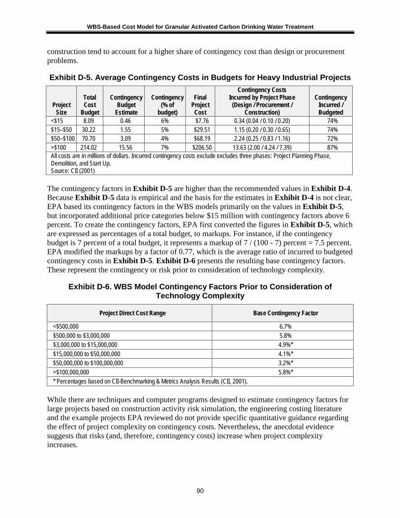
WBS-Based Cost Model for Granular Activated Carbon Drinking Water Treatment
90
construction tend to account for a higher share of contingency cost than design or procurement problems.
Exhibit D-5. Average Contingency Costs in Budgets for Heavy Industrial Projects
Project Size
Total Cost
Budget
Contingency Budget
Estimate
Contingency (% of
budget)
Final Project
Cost
Contingency Costs Incurred by Project Phase
(Design / Procurement / Construction)
Contingency Incurred / Budgeted
<$15 8.09 0.46 6% $7.76 0.34 (0.04 / 0.10 / 0.20) 74% $15–$50 30.22 1.55 5% $29.51 1.15 (0.20 / 0.30 / 0.65) 74% $50–$100 70.70 3.09 4% $68.19 2.24 (0.25 / 0.83 / 1.16) 72% >$100 214.02 15.56 7% $206.50 13.63 (2.00 / 4.24 / 7.39) 87% All costs are in millions of dollars. Incurred contingency costs exclude excludes three phases: Project Planning Phase, Demolition, and Start Up. Source: CII (2001)
The contingency factors in Exhibit D-5 are higher than the recommended values in Exhibit D-4. Because Exhibit D-5 data is empirical and the basis for the estimates in Exhibit D-4 is not clear, EPA based its contingency factors in the WBS models primarily on the values in Exhibit D-5, but incorporated additional price categories below $15 million with contingency factors above 6 percent. To create the contingency factors, EPA first converted the figures in Exhibit D-5, which are expressed as percentages of a total budget, to markups. For instance, if the contingency budget is 7 percent of a total budget, it represents a markup of 7 / (100 - 7) percent = 7.5 percent. EPA modified the markups by a factor of 0.77, which is the average ratio of incurred to budgeted contingency costs in Exhibit D-5. Exhibit D-6 presents the resulting base contingency factors. These represent the contingency or risk prior to consideration of technology complexity.
Exhibit D-6. WBS Model Contingency Factors Prior to Consideration of Technology Complexity
Project Direct Cost Range Base Contingency Factor
<$500,000 6.7% $500,000 to $3,000,000 5.8% $3,000,000 to $15,000,000 4.9%* $15,000,000 to $50,000,000 4.1%* $50,000,000 to $100,000,000 3.2%* >$100,000,000 5.8%* * Percentages based on CII-Benchmarking & Metrics Analysis Results (CII, 2001).
While there are techniques and computer programs designed to estimate contingency factors for large projects based on construction activity risk simulation, the engineering costing literature and the example projects EPA reviewed do not provide specific quantitative guidance regarding the effect of project complexity on contingency costs. Nevertheless, the anecdotal evidence suggests that risks (and, therefore, contingency costs) increase when project complexity increases.

WBS-Based Cost Model for Granular Activated Carbon Drinking Water Treatment
91
Among the WBS technologies, project complexity depends on the type of technology employed and the general degree of experience with the technology as it will be applied. Well-established technologies, which have a depth of construction and technology installation and operational history under a variety of conditions, are expected to have low risk with respect to unforeseen problems during construction and installation. Recently developed technologies or ones that have had limited application to a variety of water quality conditions and project sizes (or to the conditions at the project in question) are expected to have a higher degree of risk.
To account for differences in contingency values associated with technology type and project complexity, EPA identified four categories of project complexity and assigned multipliers that the models use to adjust the contingency factors (up or down) from Exhibit D-6:
• Low complexity = base contingency factor x 0.5 • Average complexity = base contingency factor x 1.0 • High complexity = base contingency factor x 1.5 • Very high complexity = base contingency factor x 2.0.
Thus, for each technology, the applied contingency factor combines the effects of project size and technology complexity to obtain the project specific contingency factor. EPA assigned a project complexity category to each WBS technology based on general knowledge and the application history of the technology to drinking water treatment. Exhibit D-7 shows this default complexity category assignment. The user can change these values on the indirect assumptions sheet of each model if specific knowledge of the technology and its expected performance under the site-specific conditions warrant such a change.
The WBS models assume that contingency costs are incurred only in high cost scenarios (see Section 2.3). For low and medium cost estimates, the models assume construction is completed with a minimum of unforeseen site-specific costs and, therefore, that none of the contingency budget is incurred. Users can change this assumption on the indirect assumptions sheet of each model.

WBS-Based Cost Model for Granular Activated Carbon Drinking Water Treatment
92
Exhibit D-7. WBS Default Complexity Factors by Technology
Technology Risk Level Assigned to
Technology Default Complexity
Factor Acid Feed Low 0.5 Cation Exchange Low 0.5 Caustic Feed Low 0.5 Nontreatment Options Low 0.5 Potassium Permanganate Addition Low 0.5 Granular Activated Carbon Average 1 Chlorine Gas Average 1 Packed Tower Aeration Average 1 Adsorptive Media High 1.5 Anion Exchange High 1.5 Biological Treatment High 1.5 Microfiltration and Ultrafiltration High 1.5 Greensand Filtration High 1.5 Hypochlorite Addition High 1.5 Multi-stage Bubble Aeration High 1.5 Reverse Osmosis and Nanofiltration High 1.5 Ultraviolet Advanced Oxidation Processes Very high 2 Ultraviolet Disinfection Very high 2
D.13 Miscellaneous Allowance In a cost estimate for a construction project, an allowance may be included for conditions or events that the estimator can anticipate, but whose cost is not known with any degree of certainty. If, for example, the site is expected to have contaminated soil that may require remediation, the allowance will incorporate the resulting costs. An allowance differs from a contingency cost, which provides contract coverage for unpredictable conditions. The allowance funds account for anticipated additional costs that should become apparent at a later stage of the project (for example, upon completion of the site investigation activities and the detailed engineering design). Much of this cost is associated with knowledge of site-related conditions.
In a national average cost estimate such as the one that the WBS models generate, it is not possible to allow for the specific conditions associated with any given site. However, the models include an allowance line item to simulate an average effect due to such conditions. The line also accounts for the level of detail in the WBS design, since the models do not include all minor process components.
The WBS models assume a miscellaneous allowance of 10 percent as a default. Since the allowance addresses a modeling uncertainty, there is little guidance available from the cost estimation literature. Instead, the assumption must be validated by comparing WBS output to actual water treatment facility construction costs. Users can change the miscellaneous allowance on the indirect assumptions sheet of each model.

WBS-Based Cost Model for Granular Activated Carbon Drinking Water Treatment
93
D.14 Legal, Fiscal and Administrative This category includes project management, accounting and administrative activities related to the project, excluding permitting. The cost can range from 2 to 5 percent of the process cost. In the WBS models, this category is considered to account for administrative costs that the purchaser incurs in the course of procurement. These costs are distinct from the construction management fee, which is included as a separate indirect cost (Section D.17). The WBS models use a default value of 2 percent. Users can change this assumption on the indirect assumptions sheet of each model.
D.15 Sales Tax Water treatment plant projects may be exempt from the sales tax, particularly those constructed with public funds. The default value in the WBS models is 0 percent, which reflects the status of taxes in social cost analysis. Taxes are considered a transfer payment and not an actual social cost, which is based on the concept of opportunity cost. Transfer payments are not included in social cost analysis, so a default value of 0 percent is appropriate for social cost analysis. The WBS models include a sales tax line item among indirect costs because the models can also be used for private cost analysis (e.g., for a specific utility), which includes transfer payments. Users can enter a sales tax percentage on the indirect assumptions sheet of each model in cases where consideration of transfer payments is appropriate.
D.16 Financing During Construction Engineering cost estimates include interest for financing of the project. Drinking water systems can obtain financing through various sources including Drinking Water State Revolving Funds (DWSRF), public-sector financing, private-sector borrowing or equity instruments. Exhibit D-8 shows interest rates for drinking water treatment projects derived from the EPA 2006 Community Water Systems Survey. The default value in the WBS models is 5 percent, which is toward the higher end of the range of financing costs for public and private systems, and implicitly assumes 1 year of financing during construction. For small systems with design flow less than 1 MGD, the models assume 0 percent financing during construction, implicitly accounting for the very short construction time required for these systems. Users can change the assumptions for both large and small systems on the indirect assumptions sheet of each model.

WBS-Based Cost Model for Granular Activated Carbon Drinking Water Treatment
94
Exhibit D-8. Average Interest Rates for Capital Funds
System Ownership Type and Lender Average Interest Rate (All System Sizes) Range of Average Interest Rates
Public Systems DWSRF 2.3 1.0 – 3.5 Other Public Sector 3.5 0.5 – 4.4 Private Sector 4.6 4.2 – 5.0 Other 3.9 0.0 – 4.9
Private Systems DWSRF 5.6 0.8 – 6.2 Other Public Sector 4.4 3.1 – 5.5 Private Sector 6.5 4.3 – 7.7 Other 5.9 0.0 – 10.0
All Systems DWSRF 2.6 1.0 – 4.3 Other Public Sector 3.8 1.9 – 4.5 Private Sector 5.2 4.3 – 5.5 Other 4.3 0.0 – 10.0
All Systems and Lenders 0.0 – 10.0 D.17 Construction Management and General Contractor Overhead As discussed in Section D.4.2, the component costs in the WBS cost database include the cost of installation, including O&P for the installing contractor. However, the installation cost does not cover the cost of insurance, performance bonds, job supervision or other costs associated with the general contractor. The WBS models account for these costs by combining costs and fees for the following items:
• Builder’s risk insurance • Performance bonds • Construction management.
Builder’s risk insurance is casualty insurance for the project during construction and may cover various risks, such as vandalism, fire, theft or natural disasters. According to RSMeans (2009c), a national average rate is 0.34 percent of the project cost. EPA adopted this assumption for the WBS models. Users can adjust this rate on the indirect assumptions sheet of each model.
Performance bonds compensate the owner for losses due to contractor failure to complete work according to specifications. RSMeans (2006) estimates the costs based on the total direct cost of the project, as described in Exhibit D-9.

WBS-Based Cost Model for Granular Activated Carbon Drinking Water Treatment
95
Exhibit D-9. Cost of Performance Bonds
Project Direct Cost Range Performance Bond Cost
<$100,000 2.5% $100,000 to $500,000 $2,500 plus 1.5% of the amount over $100,000
$500,000 to $2,500,000 $8,500 plus 1.0% of the amount over $500,000 $2,500,000 to $5,000,000 $28,500 plus 0.75% of the amount over $2,500,000 $5,000,000 to $7,500,000 $47,250 plus 0.70% of the amount over $5,000,000
>$7,500,000 $64,750 plus 0.60% of the amount over $7,500,000 Source: RSMeans (2006), reference table R013113-80.
The construction management fee is paid to the general contractor and covers the cost of job supervision, an on-site office, main office overhead and profit. Various sources provide individual estimates for these items, but the WBS models roll them into a construction management fee to reflect a cost structure that the owner might see. RSMeans (2009c) provides a table of typical construction management rates for jobs of various sizes. EPA adapted those rates to develop those shown in Exhibit D-10.
Exhibit D-10. Construction Management Fees
Project Direct Cost Range Construction Management Fee
<$100,000 10% $100,000 to $250,000 9%
$250,000 to $1,000,000 6% $1,000,000 to $5,000,000 5%
$5,000,000 to $10,000,000 4% >$10,000,000 3.2%a
a. The reference quotes a fee range of 2.5% to 4% for a $50 million project. The WBS models assume an intermediate rate for projects over $10 million. Source: RSMeans (2009c), division 01 11 31.20.
The indirect line item for construction management and general contractor overhead sums all of these costs. The costs can be omitted individually on the indirect assumptions sheet of each model, either by an assumption that directly controls inclusion or exclusion or by setting the appropriate percentage to zero. For example, in the case of small systems that use pre-engineered package treatment plants, the models exclude the construction management fee portion by default and include only the performance bond and builder’s risk insurance. Because package plants typically are skid-mounted and assembled offsite, they typically do not require a general contractor to supervise their installation. Instead, their installation is managed by a single entity, often the vendor that supplied the package.
D.18 City Index This indirect cost accounts for city-specific and regional variability in materials and construction costs. The city index factor included in the WBS models is expressed as a decimal number, assuming a national average of 1.0. The default value in the WBS models is set to the national

WBS-Based Cost Model for Granular Activated Carbon Drinking Water Treatment
96
average of 1.0, which is appropriate for estimating national compliance costs. Users wishing to adjust estimated costs to be more reflective of potential costs in specific geographic locations can change the city index value on the output sheet. For example, to estimate costs for a city where construction costs are 90 percent of the national average, the user would change the city index to 0.9. One source for region- or location-specific adjustment factors is RSMeans (2013), which publishes average construction cost indices for various three-digit zip code locations.
D.19 List of Abbreviations and Symbols in this Appendix DWSRF Drinking Water State Revolving Funds EPA U.S. Environmental Protection Agency ENR Engineering News-Record ft2 square feet I&C instrumentation and control KW kilowatt LTL less than a load MGD million gallons per day O&P overhead and profit WBS work breakdown structure D.20 References Association for the Advancement of Cost Engineering International (AACEI). 1996. Certification Study Guide. Morgantown, West Virginia.
Allis, William A. 2005. Personal communication with L. Petruzzi, SAIC. April.
Air Force Combat Climatology Center (AFCCC). 2000. Engineering Weather Data: 2000 International Edition. Published by the National Climatic Data Center.
American Water Works Corporation (AWWC). 1999. Preliminary Cost Estimate Summary: Alton Water Treatment Plant, H&S no. 1862. 7 January.
AWWC. 2001a. Seymour, Indiana Process Cost Estimate.
AWWC. 2001b. St. Joseph, Missouri Cost Estimate.
Burger, Riaan. 2003. “Contingency, Quantifying the Uncertainty.” Cost Engineering 45, no. 8. 8 August.
California Department of Transportation (CADOT). 2001. Earth Pressure Theory and Application.
Construction Industry Institute (CII). 2001. Benchmarking & Metrics Analysis Results. Austin, Texas. May.
Fairfax Water Authority (FWA). 2003. New Construction Works Brochures. Virginia.
WBS-Based Cost Model for Granular Activated Carbon Drinking Water Treatment
97
GeoEconomics Associates Incorporated. 2002. An Economic Analysis of Water Services. Chapter 5.
Krynine, D.P. and W.R. Judd. 1957. Principles of Engineering Geology and Geotechnics. McGraw-Hill. New York.
Minnesota Natural Resources Conservation Services (MN NRSC). 2003. General Guide for Estimating Moist Soil Density. 10 May.
National Renewable Energy Laboratory (NREL). 2003. Gas-Fired Distributed Energy Resource Technology Characterizations. U.S. Department of Energy.
RSMeans. 2006. Facilities Construction Cost Data. 21st Annual Edition. Kingston, Massachusetts: RSMeans Company.
RSMeans. 2009a. Assemblies Cost Data. 34th Annual Edition. Kingston, Massachusetts: RSMeans Company.
RSMeans. 2009b. Building Construction Cost Data. 67th Annual Edition. Kingston, Massachusetts: RSMeans Company.
RSMeans. 2009c. Facilities Construction Cost Data. 24th Annual Edition. Kingston, Massachusetts: RSMeans Company.
RSMeans. 2013. Facilities Construction Cost Data 2014. 29th Annual Edition. Norwell, Massachusetts: Reed Construction Data LLC.
Scoutten, Inc. 2009. Opinion of Probable Cost for Town Of Buckeye Water And Wastewater Infrastructure and Water Resources Improvements Associated with 2009 Development Fees. Revised 11 May. Online at http://www.buckeyeaz.gov/DocumentView.aspx?DID=640
Stone and Webster. 2001. Brayton Point Station Permit Renewal Application. Five Volumes.
Tampa Bay Water. 2006. West Pasco Infrastructure Project, Maytum WTP Modifications, Project No. 05903. Memorandum from Kenneth R. Herd, Director of Operations and Facilities, to Jerry L. Maxwell, General Manager. 1 December.
United States Army Corp of Engineers (U.S. ACOE). 1992. Revision of Thrust Block Criteria in TM 5-813-5/AFM 88-10 VOL. 5 Appendix C. Publication Number: ETL 1110-3-446. 20 August.
U.S. Environmental Protection Agency (U.S. EPA). 2004. Capital Costs of Arsenic Removal Technologies, U.S. EPA Arsenic Removal Demonstration Project, Round 1. EPA-600-R-04-201. Cincinnati, OH: U.S. EPA, National Risk Management Research Laboratory.

WBS-Based Cost Model for Granular Activated Carbon Drinking Water Treatment
98
Appendix E. General Assumptions for Operating and Maintenance Costs
E.1 Introduction The work breakdown structure (WBS) models calculate operating and maintenance (O&M) costs independently for each treatment technology. Nevertheless, there are several general assumptions and estimation functions that are common to the O&M estimates across the treatment models. This appendix describes those assumptions and functions. Any O&M cost element that is technology-specific is included in the chapter describing that technology in the main document.
The O&M costs estimated in the WBS models primarily include annual expenses for:
• Labor to operate and maintain the new treatment equipment • Chemicals required by the treatment • Materials needed to carry out maintenance (including small tools) • Energy.
Costs for commercial liability insurance, inspection fees, domestic waste disposal, property insurance and other miscellaneous expenditures that are not directly related to the operation of the technology are included in the WBS models by applying a miscellaneous allowance to the total annual O&M costs. This calculation uses the same miscellaneous allowance percentage that is applied to capital costs as an indirect line item (see Appendix D). Users can change this percentage on the indirect assumptions sheet of each model.
The WBS models calculate O&M costs based on the inputs provided by the user on the input sheet and values specified on the O&M assumptions sheet. These inputs include system size, raw and finished water quality parameters and other factors that affect operation requirements such as an option in the activated alumina model to regenerate media or operate on a throw away basis. The design equations and assumptions incorporated in the O&M sheets are described below.
Despite provisions for user inputs, there are several factors that can affect site-specific O&M costs in ways that are not readily reflected in the WBS outputs. These include:
• Operator expertise • Equipment quality, design, installation and degree of automation • Environmental conditions (e.g., changes in raw water quality over time).
Some O&M costs components, such as energy for pumping water or chemicals for treatment, are well defined and readily estimated using an engineering cost approach. Other O&M cost drivers, however, depend on multiple factors that are difficult to quantify and, therefore, represent a challenge for estimating costs. For example, the required level of effort to operate or maintain a technology depends on the level of complexity and sophistication of the installed technology, the size of the treatment system, the professional level or education and training of the operator and state and local regulations for process staffing.

WBS-Based Cost Model for Granular Activated Carbon Drinking Water Treatment
99
To complicate matters further, there are trade-offs between system capital costs and O&M costs. Higher cost equipment may require less intensive maintenance or less hands-on operation. For example, using mixers and tanks to prepare brine solution for regenerating an anion exchanger might reduce equipment costs compared to using salt saturators. However, salt saturators require less labor to use and potentially reduce the need for a salt storage facility. Also high quality, highly automated systems can significantly reduce labor requirements, but increase capital costs. The U.S. Environmental Protection Agency (EPA) included some adjustments to O&M costs in the WBS models to account for some types of savings, which are described below.
E.2 Labor Costs The WBS models calculate the annual hours of O&M labor in the following categories:
• Operator labor for operation and maintenance of process equipment • Operator labor for building maintenance • Managerial and clerical labor.
The WBS model labor hour estimates are intended to be incremental. That is, they only include labor associated with the new treatment system components.
E.2.1 Operator Labor for Operation and Maintenance of Process Equipment System operation includes the following primary tasks:
• Collecting data from process instruments and recording system operating parameters • Preventative maintenance and calibration of process instruments • Verifying the proper operation of pumps, valves and other equipment and controlling the
treatment process by adjusting this equipment • Preventative maintenance of pumps, valves and other equipment • Inspection and maintenance of chemical supplies • Visual inspection of the treatment facility and system components • Other, technology-specific tasks (e.g., managing regeneration, backwash or media
replacement).
Labor required for these tasks is sensitive to the level of system automation. As discussed in Section 2.3 and Appendix A, the user has the option to choose from three levels of automation: manual, semi-automated and fully automated. The assumptions about labor required for each task vary depending on the level of automation selected, as shown in Exhibit E-1 and discussed below. Users can change these assumptions, if desired, on the O&M assumptions sheet of each model.
EPA compared model results using these assumptions with annual labor hours reported for 12 different water treatment facilities. Most of the resulting model estimates were within +50 percent to -30 percent of the annual labor hours reported for the sample facilities.

WBS-Based Cost Model for Granular Activated Carbon Drinking Water Treatment
100
Exhibit E-1. Operator Labor Assumptions for Three Levels of Automation
Task Manual Semi-automated Automated
Record system operating parameters from process instruments (includes routine sampling)
5 minutes per day per instrument 5 minutes per day 5 minutes per day
Preventative maintenance and calibration of process instruments
10 minutes per month per instrument
10 minutes per month per instrument
10 minutes per month per instrument
Verify and adjust pump operating parameters 5 minutes per day per pump
5 minutes per day per pump None
Preventative maintenance of pumps 30.25 hours per year per pump
30.25 hours per year per pump
30.25 hours per year per pump
Verify and adjust valve positions 5 minutes per week per valve
5 minutes per week per valve None
Preventative maintenance and inspection of valves 5 minutes per year per valve
5 minutes per year per valve
5 minutes per year per valve
Visual inspection of facility 1 minute per day per 100 square feet of facility
1 minute per day per 100 square feet of facility
1 minute per day per 100 square feet of
facility
Inspect and maintain chemical supplies 60 minutes per
month per chemical supply
tank
60 minutes per month per
chemical supply tank
60 minutes per month per chemical supply
tank
Collecting Data from Process Instruments and Recording System Operating Parameters For manual systems, the models assume 5 minutes per day per instrument associated with day-to-day operation of the treatment process (e.g., flow meter, head loss sensor). Instruments associated with intermittent processes (e.g., backwash flow meters) are not included in this estimate, because observation of these instruments is included the operator labor associated with managing the intermittent process. In semi-automated and automated systems, the control system handles the task of collecting information from the various process instruments, so operator labor is reduced to 5 minutes per day to keep a record of operating parameters.
Preventative Maintenance and Calibration of Process Instruments Regardless of the level of automation, the models assume 5 minutes per month for each instrument, including those associated with intermittent processes. While some instruments (e.g., chlorine residual analyzers) may require calibration more frequently than monthly, others (e.g., head loss sensors) will require limited, less frequent maintenance. Therefore, the models use 10 minutes per month as an average across the various types of instruments.
Verify and Adjust Pump Operating Parameters For manual and semi-automated systems, the models assume 5 minutes per day per pump, including metering pumps associated with continuous chemical feed processes. Pumps associated with intermittent processes (e.g., backwash pumps) are not included in this estimate,

WBS-Based Cost Model for Granular Activated Carbon Drinking Water Treatment
101
because operation of these pumps is included the operator labor associated with managing the intermittent process. In automated systems, the control system handles this task, so no additional operator labor is required.
Preventative Maintenance of Pumps Regardless of level of automation, the models assume 30.25 hours per year for large, frequently operated pumps (e.g., booster pumps). This estimate does not include small chemical metering pumps, but does include backwash pumps when these are operated more frequently than weekly. The estimate of 30.25 hours per year is based on a list of recommended pump maintenance activities from a vendor and the assumptions for each activity shown in Exhibit E-2.
Exhibit E-2. Pump Maintenance Activities
Task Interval Estimated Minutes/Task Estimated Hours/Year
Check bearing temperature Monthly 5 1
Changing lubricant/ adjusting power level Monthly 30 6
Disassemble for inspection, reassemble Monthly 60 12
Check oil Quarterly 10 0.67
Check lubricated bearings for saponification Quarterly 10 0.67
Removal of bearings and replace, reassemble Quarterly 60 4
Check packing and replace if necessary, reassemble 6 months 60 2
Vibration readings 6 months 10 0.33
Remove casing and inspect pump Annual 120 2
If parts are worn, replace Annual varies covered by pump materials percentage and pump
useful life
Clean deposits and/ or scaling Annual 60 1
Clean out stuffing box piping Annual 30 0.5
Measure and record suction and discharge pipe head Annual 5 0.08
Total Hours/Year: 30.25 Verify and Adjust Valve Positions For manual and semi-automated systems, the models assume 5 minutes per week per valve on the main process line. In automated systems, the control system handles this task, so no additional operator labor is required.
Preventative Maintenance and Inspection of Valves Regardless of level of automation, the models assume 5 minutes per year per valve on the main process line.

WBS-Based Cost Model for Granular Activated Carbon Drinking Water Treatment
102
Visual Inspection of Facility Regardless of level of automation, the models assume 1 minute per week per 100 square feet (ft2) of treatment system floor plan to conduct visual inspection of the overall process. This daily inspection is in addition to inspection conducted as part of routine operation and maintenance of major operational components (instruments, pumps and valves), as discussed above.
Inspect and Maintain Chemical Supplies The models assume that chemical supplies, whether they are associated with continuous addition or intermittent use, require additional attention beyond that included in daily visual inspection. In particular, they also require labor associated with receiving chemical shipments. Regardless of level of automation, the models assume 60 minutes per month for each chemical storage tank. Although counted on the basis of the number of tanks, this estimate is intended to cover all components associated with the chemical supply system (e.g., checking pipes and valves for leaks and inspecting and maintaining small metering pumps).
Technology-Specific Tasks Many of the technologies include activities in addition to day-to-day operation that may require operator attention, depending on the level of automation (e.g., intermittent regeneration, backwash or media replacement). Where this is the case, the technology chapters in the main document describe the specific assumptions required to calculate operator labor.
E.2.2 Labor for Building Maintenance The WBS models include a building maintenance cost based on the building area (i.e., using a unit cost in dollars per square foot per year). EPA developed this cost based on two sources: Whitestone Research (2009) and RSMeans (2013). Specifically, EPA selected a list of appropriate building maintenance repair and repair tasks from those listed in the two sources. The selected tasks include those associated with preventative maintenance, small repairs and major repairs. EPA estimated a frequency for each task by averaging the frequency recommended in each of the two sources. Exhibit E-3 identifies the tasks included in the maintenance and repair buildup. The models include maintenance and repair tasks for heating and cooling systems only for buildings with the relevant systems. To avoid double-counting, the task list does include tasks in the following categories:
• Maintenance of treatment system components that are already explicitly considered in the models’ maintenance labor and materials costs (e.g., pumps, valves, instruments)
• Full replacement of items that are explicitly given a useful life in the models (e.g., piping, heating and cooling systems)
• Repair tasks with a lower frequency than the useful life assumed in the models for the related WBS line item (e.g., skylight replacement has a recommended frequency of 40 years, whereas the models assume a useful life for the entire building of 37 to 40 years).
For the buildup, EPA assumed a baseline building area of 4,000 ft2 and building components corresponding to a medium-quality building (see the assumptions in Appendix B). EPA estimated costs for each task using data from RSMeans (2013) and assuming that preventative maintenance and minor repairs would be conducted using in-house labor, while major repairs would be conducted using outside contractors. These costs include both labor and materials.

WBS-Based Cost Model for Granular Activated Carbon Drinking Water Treatment
103
Because repair needs do not follow a strict schedule, EPA annualized costs with no discount rate—that is, a $100 task with a typical frequency of 5 years is assigned an annual cost of $20.
Labor accounts for most of the cost for the maintenance and repair tasks. Further, the Building Cost Index and Construction Cost Index, the only two cost indices in the WBS cost database that combine labor and material costs, do not include the costs of materials that are likely to be used in building maintenance. The WBS cost database therefore uses the Employment Cost Index to escalate the building maintenance costs to current year dollars.
Exhibit E-3. Building Maintenance and Repair Tasks • Minor repairs and refinishing for concrete floors • Repairs and waterproofing for exterior concrete block walls • Repairs and refinishing for doors • Roofing debris removal and inspections • Minor repairs and replacement for roofing membranes and flashing • Repairs to skylights • Repairs and refinishing for interior concrete block walls • Repairs and refinishing for drywall • Office painting • Vinyl tile flooring replacement • Repairs, refinishing and replacement for acoustic tile ceilings • Preventive maintenance, repairs and replacement for lavatories and lavatory fixtures • Water heater preventive maintenance, cleaning and servicing, overhauls and replacement • Repairs to pipe joints and fittings • Cleaning of drains • Maintenance, repair and replacement of gutters • Repair and replacement of fans • Inspection and replacement of sprinkler systems • Maintenance, inspection, repair and replacement of electrical systems including switchgear, receptacles, wiring devices,
voice/data outlets and structure ground • Replacement of lamps, ballasts and lighting fixtures • Standby generator maintenance and inspection • Preventive maintenance of computers E.2.3 Managerial and Administrative Labor The models contain an assumption that managerial and administrative support levels for a new treatment plant are equal to 10 percent of the total operator hours for system operation and maintenance. This estimate is not intended to represent total administrative and managerial time at a drinking water system, because total time includes many tasks unrelated to operating a new treatment train. It only represents incremental time needed to provide administrative support for the new treatment plant, e.g., processing supply orders. It also does not include labor time associated with recordkeeping and reporting burden estimates that EPA must estimate and report independently to comply with Paperwork Reduction Act requirements. Users can change the 10

WBS-Based Cost Model for Granular Activated Carbon Drinking Water Treatment
104
percent assumption for either or both of managerial and administrative labor on the O&M assumptions sheet of each model.
E.2.4 Labor Unit Costs To estimate the cost of the labor calculated in each of the categories above, the models multiply labor hours by unit costs from the WBS cost database. These unit costs reflect average loaded wage rates for applicable labor categories (i.e. technical, managerial and administrative) and vary across system size. The WBS cost database uses the Employment Cost Index to escalate the rates to current year dollars. Users can change the wage rates, if desired, in the WBS cost database.
E.3 Chemicals Each of the WBS models calculates annual chemical usage (in pounds or gallons per year) on a technology-specific basis. The technology chapters in the main document describe these calculations. In some models, these calculations also reflect the selected option for regeneration or disposal of spent chemicals. Annual chemical costs equal the product of the annual chemical requirements and the unit chemical costs in the WBS cost database.
E.4 Materials The WBS models calculate the annual cost of materials in the following categories:
• Materials for maintenance of booster or influent pumps • Materials for maintenance and operation of other, technology-specific equipment • Replacement of technology-specific equipment that occurs on an annual basis • Materials for building maintenance.
Pumps are operated continuously (or nearly continuously) and require preventive and routine maintenance. Pumps are common to all the technologies. Each of the models assumes the annual cost of materials for pumps is equal to 1 percent of their pre-installation capital cost to account for consumable supplies and small parts requiring frequent replacement. This assumption is based on input from the technology experts who reviewed the WBS models and commented that the initial assumption of 5 percent was too high. Users can change this assumption on the O&M assumptions sheet of each model. Although accidents or improper operation can result in a need for major repairs that increase maintenance materials costs beyond 1 percent, the models do not include these types of costs.
Some of the technologies include other equipment that may require significant maintenance (e.g., the blowers in the packed tower aeration and multi-stage bubble aeration technologies). The models for these technologies include annual costs for maintenance materials. The technology chapters in this document describe the specific calculations. In general, these calculations are based a percentage of the pre-installation capital cost of the equipment.
Some of the technologies also include equipment components (e.g., membrane filter cartridges) that require frequent replacement. Rather than treat these components as frequently replaced capital items, the models handle the replacement costs in the O&M sheet. The replacement cost calculations are based on assumptions about replacement frequency and unit costs from the WBS

WBS-Based Cost Model for Granular Activated Carbon Drinking Water Treatment
105
component cost database. The specific calculations are in the technology sections of the main document.
The WBS models compute a cost for building maintenance that combines labor and materials. The cost is discussed in Section E.2.2.
E.5 Energy All of the WBS models calculate the annual cost of energy in the following categories:
• Energy for operation of booster or influent pumps • Energy for operation of other, technology-specific items of equipment • Energy for lighting • Energy for ventilation • Energy for cooling • Energy for heating.
E.5.1 Energy for Pumps and Other Equipment Booster or influent pumps are equipment common to all the technologies. Because these pumps are operated continuously (or nearly continuously), they can represent significant energy consumption. Therefore, each of the WBS models calculates pump operating horsepower based on average flow, pump head and pump efficiency. The models then convert this operating horsepower to megawatt-hours/year assuming continuous operation. To calculate annual cost, the models then multiply the annual power requirement by the unit cost for electricity contained in the WBS component cost database.
Some of the technologies include other equipment that consumes significant quantities of energy (e.g., blowers, backwash pumps, mixers). For those technologies, the model also calculates the energy for such equipment explicitly. The technology chapters in the main document describe the specific energy calculations. In general, those calculations are similar to the energy calculation for pumps.
E.5.2 Energy for Lighting The models calculate annual lighting requirements based on the building square footage estimate and the quality level of the building (see Appendix B). The building capital costs in the WBS cost database include the cost of light fixtures for the following light requirements:
• Sheds and low quality buildings, 1 watt/hour/ft2 of building area • Mid quality buildings, 2 watts/hour/ft2 of building area • High quality buildings, 4 watts/hour/ft2 of building area.
Multiplying the appropriate light requirement by 8.8 results in an energy usage rate in kilowatt hours per ft2 per year. This conversion is based on operation of the lights 24 hours per day, 365 days per year. EPA evaluated these assumptions by calculating the granular activated carbon contactor, pipe gallery and furnace area lighting requirements at the Richard Miller Water Treatment Plant in Cincinnati, Ohio. For this facility, the lighting requirements are 1.5, 1.0 and 0.8 watts per hour per ft2 for the contactor, pipe gallery and regeneration areas, respectively, with

WBS-Based Cost Model for Granular Activated Carbon Drinking Water Treatment
106
a weighted average of 1.0 watt per hour per ft2, which is at the low end of the range that EPA uses in the models. Technologies with different types of process equipment that require more frequent access may require more lighting. Users can change the lighting requirement for each level of building quality on the O&M assumptions sheet of each model.
Because many systems are not lit during times an operator is not present, the models reduce lighting energy requirements when a full-time operator presence is not required (possible for small systems for many technologies) using the following factor (with a maximum of 1 to account for large systems that might require more than one full-time operator):
Operator hours per year/ (24*365).
E.5.3 Energy for Ventilation The models calculate ventilation requirements based on the assumptions shown in Exhibit E-4. The technology experts who reviewed the assumptions for the WBS models confirmed the reasonableness of these assumptions, although one expert commented that the air change rate for pumps could be lower for systems in a northern climate. The WBS models continue to use the value shown, however, because it is believed to be more reasonable for a national average estimate and results in a more conservative (i.e., higher) estimate of ventilation energy consumption. All of the models use these same assumptions with the exception of chlorination, which has special ventilation requirements as described in that technology section. Users can change the ventilation assumptions, if desired, on the O&M assumptions sheet of each WBS technology model.
Exhibit E-4. Assumptions for Calculating Ventilation Requirements Variable Value used
Ventilation air change rate for contactor areas 3 air changes/hour
Ventilation air change rate for pump areas 20 air changes/hour
Ventilation air change rate for chemical storage areas 2 air changes/hour
Ventilation air change rate for offices 2 air changes/hour
Pressure drop across ventilation fans 0.25 pounds/ ft2
Number of days with mechanical ventilation for small systems (less than 1 MGD) 90 days/year
Number of days with mechanical ventilation for medium systems (1 to 10 MGD) 120 days/year
Number of days with mechanical ventilation for large systems (greater than 10 MGD) 185 days/year
Building height 20 feet
MGD = million gallons per day The models first use the air change rate assumptions to calculate an overall weighted average air change rate for each building based on the equipment present in that building. The models then use this weighted average air change rate for each building in the following formula:
Ventilation energy (MWh/yr) = DAYS × 24 × 0.746 × Pdrop × FP × H × Achanges / 33,000,000

WBS-Based Cost Model for Granular Activated Carbon Drinking Water Treatment
107
where: DAYS = days per year with mechanical ventilation Pdrop = pressure drop across ventilation fans (pounds/ft2) FP = building footprint (ft2) H = building height (feet) Achanges = weighted average air change rate for the building (air changes/hour)
E.5.4 Energy for Heating and Cooling The models calculate heating and cooling requirements based on the assumptions shown in Exhibit E-5. Users can change these assumptions, if desired, on the O&M assumptions sheet of each WBS technology model. These assumptions are described in greater detail below.
R-values are a measure of the effective resistance to heat flow of an insulating barrier such as a building envelope. The R-values assumed in the models (13 for walls, 38 for ceilings) are based on the use of standard building materials. The user can change these values to reflect higher efficiency construction materials. In doing so, however, the user should also examine the unit building costs in the WBS cost database (see Appendix B) to determine if they are consistent with the use of such construction materials.

WBS-Based Cost Model for Granular Activated Carbon Drinking Water Treatment
108
Exhibit E-5. Assumptions for Calculating Heating and Cooling Requirements Variable Value used
R-value for walls 13 hour - ft2 - oF /BTU
R-value for ceilings 38 hour - ft2 - oF /BTU
Annual heating degree days 4,923 degree days
Annual cooling degree days 1,697 degree days
Heating ventilation/infiltration load 168,679 BTU/cfm
Cooling ventilation/infiltration load 51,771 BTU/cfm
Electric resistance heating efficiency 98%
Heat pump heating coefficient of performance 3.2
Natural gas non-condensing furnace efficiency 80%
Natural gas condensing furnace efficiency 95%
Diesel non-condensing furnace efficiency 78%
Diesel condensing furnace efficiency 85%
Air conditioning energy efficiency ratio 11 Whr/BTU
Heat pump cooling energy efficiency ratio 10.1 Whr/BTU
Maximum capacity for heat pump heating 200 thousand BTU per hour
Maximum capacity for other heating options 6,148 thousand BTU per hour
Maximum capacity for heat pump cooling 50 tons
Maximum capacity for other cooling options 113.32 tons BTU = British thermal unit cfm = cubic feet per minute Whr = watt hour
The next four values in the exhibit (annual heating and cooling degree days and heating and cooling ventilation/infiltration loads) are climate-related. EPA derived these values from data in the Air Force Combat Climatology Center Engineering Weather Data Version 1.0 (U.S. Air Force, 2000). Specifically, EPA selected climate data for 21 cities distributed geographically throughout the United States and calculated total annual heating and cooling losses. The values used in the WBS models are those for the city (St. Louis) that represents the median total annual heating and cooling loss from among the 21 cities. Therefore, the values used are intended to represent a climate that produces a national median total heating and cooling requirement. The user can change these values to represent a specific different climate. In doing so, however, the user should select values for the heating and cooling measures, respectively, that are consistent with one another (i.e., reflective of a realistic climate).

WBS-Based Cost Model for Granular Activated Carbon Drinking Water Treatment
109
The remaining values in the exhibit are related to the efficiency and performance of heating and air conditioning equipment. These values are based on data from the following sources:
• 10 CFR 430.32 • Canadian Office of Energy Efficiency (2009) • ACEEE (2012).
The user can modify these values, as desired, to reflect the use of more or less efficient equipment.
The WBS models use the assumptions in Exhibit E-5, along with estimated building dimensions, to calculate total annual heating and cooling losses. The models consider both conductance losses and ventilation/infiltration losses. The models calculate conductance losses for each building using the following formulae:
Conductance heating loss = 4 × S × H × HDD × 24 / Rwall + FP × HDD × 24 / Rceiling Conductance cooling loss = 4 × S × H × CDD × 24 / Rwall + FP × CDD × 24 / Rceiling
where: S = length of building side in feet (assumed to equal the square root of the building
footprint) H = building height (feet) HDD = annual heating degree-days CDD = annual cooling degree-days FP = building footprint (ft2) Rwall = R-value for walls Rceiling = R-value for ceiling.
The equations above represent the total heat transfer in British thermal units (BTU)/year through all four walls and the ceiling of each building. The models assume heat transfer through the building floor is negligible.
To calculate ventilation and infiltration losses, the models first calculate the air exchange rate in cubic feet per minute (cfm) for each building using the following formula:
Air exchange rate (cfm) = FP × H × Achanges / 60
where: H = building height (feet) FP = building footprint (ft2) Achanges = weighted average air change rate for the building (air changes/hour, as
described above in the section on ventilation)
Note that, unlike the calculation for ventilation energy use, this calculation does not incorporate assumptions about the frequency of mechanical ventilation. This is because heating and cooling losses occur regardless of whether ventilation is achieved by mechanical or natural means.
WBS-Based Cost Model for Granular Activated Carbon Drinking Water Treatment
110
The models then apply the air exchange rate calculated above to determine ventilation and infiltration losses (in BTU/year) for each building using the following formulae:
Heating ventilation and infiltration heat loss = CFM × HVIload Cooling ventilation and infiltration heat loss = CFM × CVIload
where: CFM = air exchange rate (cfm, as calculated above) HVIload = heating ventilation/infiltration load (in BTU/cfm) CVIload = cooling ventilation/infiltration load (in BTU/cfm)
The models then sum conductance losses and ventilation/infiltration losses to determine total annual heating and cooling requirements for each building. For cooling, the models add cooling required to compensate for the waste heat generated by pumps (and other technology-specific mechanical equipment).
The models then calculate heating and cooling energy consumption for each of several options using these requirements, BTU values for the appropriate fuel (i.e., electricity, natural gas or oil) and the efficiency factors shown in Exhibit E-5. For heating, the options are electric resistance heating, electric heat pump, natural gas condensing or non-condensing furnace and diesel condensing or non-condensing furnace. For cooling, the options are conventional air conditioning and electric heat pump. As indicated by the final two assumptions in Exhibit E-5, some of these options are not applicable for systems requiring large heating or cooling capacity (i.e., large systems with large buildings). Specifically, electric resistance heating and heat pumps are not useable for heating beyond a maximum capacity of 240,000 BTU/hour and heat pumps are not useable for cooling beyond this same maximum capacity. When total annual heating or cooling losses are greater than these maximum capacities, the models do not include these options among those displayed on the output sheet.
The models determine whether to include heating and cooling costs (both capital and O&M) based on building size, system design flow and user input for component level (see Section 2.3), as shown in Exhibit E-6. Users can change these assumptions on the indirect assumptions sheet of each model. When heating and/or cooling are included, the models choose among the heating and cooling system options based on the total annualized cost of each option (annual energy cost, plus capital cost of the system annualized as discussed in Section 2.4). The models select the option with the lowest annualized cost for inclusion in the system capital costs and add the corresponding annual energy cost to O&M costs.

WBS-Based Cost Model for Granular Activated Carbon Drinking Water Treatment
111
Exhibit E-6. WBS Model Assumptions Regarding Inclusion of Heating and Cooling Component Cost Level
Selected System Design Flow:
Less than 1 MGD System Design Flow: 1
to 10 MGD System Design Flow: 10
MGD or greater Buildings 500 ft2 or greater
Low Neither Heating Only Heating and Cooling Medium Heating Only Heating and Cooling Heating and Cooling
High Heating and Cooling Heating and Cooling Heating and Cooling Buildings less than 500 ft2
Low or Medium Neither Neither Heating Only High Heating Only Heating Only Heating Only
E.5.5 Energy Unit Costs To estimate the cost of the energy consumption calculated in each of the categories above, the models use unit costs from the WBS component cost database. These unit costs represent national averages for each fuel (electricity, natural gas and diesel) obtained from the U.S. Department of Energy’s Energy Information Administration. Because energy costs are highly variable, users can change these energy unit costs, if desired, in the WBS cost database.
E.6 List of Abbreviations and Symbols in this Appendix BTU British thermal unit cfm cubic feet per minute EPA U.S. Environmental Protection Agency ft2 square feet O&M operating and maintenance WBS work breakdown structure E.7 References American Council for an Energy Efficient Economy (ACEEE). 2012. Heating. Last updated December. Online at http://www.aceee.org/consumerguide/heating.htm.
Canadian Office of Energy Efficiency. 2009. Heating with Gas – Comparing Annual Heating Costs.
RSMeans. 2013. Facilities Maintenance and Repair Cost Data 2014. 21st Annual Edition. Norwell, Massachusetts: Reed Construction Data.
U.S. Air Force. 2000. Air Force Combat Climatology Center Engineering Weather Data. Version 1.0.
Whitestone Research. 2009. The Whitestone Facility Maintenance and Repair Cost Reference 2009-2010. Fourteenth Annual Edition. October.