wordperfect - sptheos · since earlier action potentials (39). possible biological substrates for...
TRANSCRIPT

neur
o-sy
s/98
1000
1 3
0 O
ct 1
998
Spike Train Metrics, RevisedVictor and Purpura 17:20 October 30, 1998
METRIC-SPACE ANALYSIS OF SPIKE TRAINS: THEORY, ALGORITHMS, AND APPLICATION
Jonathan D. Victor and Keith P. Purpura
Department of Neurology and NeuroscienceCornell University Medical College
1300 York AvenueNew York, NY 10021
Address correspondence to:
Jonathan D. VictorDepartment of Neurology and NeuroscienceCornell University Medical College1300 York AvenueNew York, New York 10021
voice: (212) 746-2343fax: (212) 746-8984email: j [email protected] .edu
running head: Spike train metrics
key words: temporal coding, metric space, dynamic programming
1

Spike Train Metrics, RevisedVictor and Purpura 17:20 October 30, 1998
ABSTRACT
We present the mathematical basis of a new approach to the analysis of temporal coding. The
foundation of the approach is the construction of several families of novel distances (metrics) between
neuronal impulse trains. In contrast to most previous approaches to the analysis of temporal coding, the
present approach does not attempt to embed impulse trains in a vector space, and does not assume a Euclidean
notion of distance. Rather, the proposed metrics formalize physiologically-based hypotheses for what aspects
of the firing pattern might be stimulus-dependent, and make essential use of the point process nature of neural
discharges. We show that these families of metrics endow the space of impulse trains with related but
inequivalent topological structures. We show how these metrics can be used to determine whether a set of
observed responses have stimulus-dependent temporal structure without a vector-space embedding. We show
how multidimensional scaling can be used to assess the similarity of these metrics to Euclidean distances. For
two of these families of metrics (one based on spike times and one based on spike intervals), we present
highly eff icient computational algorithms for calculating the distances. We ill ustrate these ideas by application
to artificial datasets and to recordings from auditory and visual cortex.
2

Spike Train Metrics, RevisedVictor and Purpura 17:20 October 30, 1998
INTRODUCTION
Recent neurophysiologic studies in vision (12, 25, 30, 33, 35, 47), audition (1, 13, 28), and olfaction
(22, 41) have provided convincing evidence that sensory information is represented by the temporal structure
of a neural discharge, as well as by the number of spikes in the response. Although a neuronal discharge is
fundamentally a point process, many approaches to the analysis of temporal structure rely on binning the spike
trains and on adopting methods appropriate for multivariate data (10) or continuous signals. There are two
potential drawbacks to such approaches (47). One problem is that an adequate time resolution over a
reasonable analysis interval requires an embedding in a high-dimensional vector space which is only sparsely
sampled by the dataset. More fundamentally, this approach is less than optimal because the vector space|
approach (i) treats all coordinates on an equal footing, and thus ignores the sequential nature of time; and (ii )|
assumes that the space of spike trains has a Euclidean geometry. One might argue that an assumption of an
underlying Euclidean geometry is justified in instances in which there is an approximately Euclidean
"perceptual space" -- such as representations of color -- but it is diff icult to justify this assumption when the
geometry of the perceptual space is unknown -- e.g., a representation of "objects".
Methods which do not require vector-space embeddings have been used to examine temporal coding,
but currently-available methods have other drawbacks. A neural network scheme (19, 28) for the
classification of spike discharges can surmount the temporal resolution problem. However, inferences
concerning the nature of the temporal code are not straightforward, since they require an understanding both
of the manner in which spike trains are represented (19) and the parameters of the neural network. Other
approaches deal explicitl y with spike trains as point processes, but these methods focus on correlations among
3

Spike Train Metrics, RevisedVictor and Purpura 17:20 October 30, 1998
discharges (31, 32), the pattern of interspike intervals (34), or the identification of similar segments of spike
discharges (3), rather than on a global analysis of how the pattern of the discharge depends on the stimulus.
We recently (47) used a novel approach to investigate temporal coding in the primate visual cortex.
One major distinction between the present approach and many previous approaches is that it provides a global
analysis of how the discharge pattern depends on the stimulus, without the need for an embedding in a vector
space, or an assumption of a Euclidean (or near-Euclidean) geometry for the set of spike trains. The
philosophy behind this approach is to exploit what is known about the biological significance of the temporal
pattern of nerve impulses to construct a specifically appropriate mathematical structure, rather than to adapt
general-purpose methods of signal processing. The purpose of this paper is to describe the mathematical basis
of this approach in detail .
4
Spike Train Metrics, RevisedVictor and Purpura 17:20 October 30, 1998
RESULTS
Overview
For the reasons described in the Introduction, we construct a method to analyze the temporal structure
of spike trains based only on the bare essentials: an abstract set of points (the spike trains) and a self-
consistent definition of distances between pairs of these points. In formal mathematical terms, we consider the
spike trains and the notion of distance to define a metric space (11), a topological structure substantiall y more
general than a vector space with a Euclidean distance. The extent to which our construct indeed corresponds
to a Euclidean distance in a vector space will be determined empirically, rather than assumed.
We will consider several families of metrics. Each metric determines a candidate geometry for the
space of spike trains. Stimulus-dependent clustering will be assessed relative to each candidate geometry,
without recourse to further mathematical structure.
The metrics we consider are based on intuitions concerning possible biological underpinnings of
temporal coding. The first family of metrics, denoted Dspike[q], emphasizes the significance of the absolute
timing of individual impulses. The rationale for this family of metrics is that under some circumstances, a
cortical neuron may behave li ke a coincidence detector (2, 27, 42, 43), but the effective resolution of this
coincidence detector is uncertain. Within the resolution of this coincidence detector, the effect of a spike train
on other cortical neurons will depend on the absolute timing of its impulses, rather than on the number of
spikes within a given interval.
5

Spike Train Metrics, RevisedVictor and Purpura 17:20 October 30, 1998
A second family of metrics, denoted Dinterval[q], emphasizes the duration of interspike intervals. The
rationale in this case is that the effect of an action potential can depend criti cally on the length of the time
since earlier action potentials (39). Possible biological substrates for this dependence include the NMDA
receptor and Ca2+ channels whose behavior is sensiti ve to the pattern of interspike intervals (6, 21, 36). While
it is triviall y true that the absolute spike times determine the interspike intervals (and vice-versa, with the
notion that the first "interspike interval" is the interval between the onset of data collection and the first
spike), it is not true that the distance between two spike trains, in the sense of Dspike, determines the distance
between the trains in the sense of Dinterval.
Finally, we will consider a third family of metrics, Dmotif, which is motivated by the notion that a
"motif," or a temporal pattern of a subset of spikes (3), may be of physiological significance. This family of
metrics is a natural formal extension of Dspike and Dinterval. However, implementation of our analysis for Dmotif
is hindered by the lack of availabilit y of eff icient algorithms.
Within each of these families, the specific metrics that we will consider (Dspike[q], Dinterval[q], and
Dmotif[q]) depend on a parameter q, which expresses the sensiti vity of the metric to temporal pattern. The
parameter q has units of (sec-1) and represents the relative cost to "move" a spike (for Dspike[q]), to change the
duration of an interval (for Dinterval[q]), or to translate a motif (for Dmotif[q]), compared to the cost of inserting
or deleting a spike. For q = 0, each of these metrics reduce to a distance based solely on counting spikes.
Thus, temporal coding will manifest itself as more reliable clustering for some values of q > 0 than for q = 0.
For suff iciently large values of q, we anticipate a decrease in systematic clustering, since the infinitesimally
precise timing of impulses or intervals cannot possibly carry biological information. Thus, our method
6

Spike Train Metrics, RevisedVictor and Purpura 17:20 October 30, 1998
provides two characterizations of temporal coding: the amount of systematic clustering seen with q > 0 will
indicate the extent to which absolute spike times (Dspike[q]), spike intervals (Dinterval[q]), or subsets of spikes
(Dmotif[q]) depend on the stimulus, and the value of q for which the clustering is greatest. The latter
characterization will i ndicate the temporal resolution of the coding.
Mathematical framework and definition of metrics
A metric space (11) is a set of points (here, spike trains, to be denoted Sa, Sb, ...) along with a metric
D, which is a mapping from pairs of spike trains to the real numbers. In order for D to be a metric, it must
(i) always be positi ve except for the trivial case D(S, S) = 0, (ii ) be a symmetric function
[D(Sa, Sb) = D(Sb, Sa)], and (iii ) satisfy the triangle inequality
(1)D(Sa, Sc) ≤ D(Sa, Sb) D(Sb, Sc) .
With these conditions satisfied, the function D can be thought of as specifying a distance.
A spike train S is a sequence of times t1, t2, ..., tk, with 0 ≤ t1 < t2 < ... < tk , and will be denoted
S = { t1, t2, ..., tk} . We will define a metric D(Sa, Sb) as the minimum "cost" required to transform the spike
train Sa into the spike train Sb via a path of elementary steps. The cost assigned to a path of steps is the sum
of the costs assigned to each of the elementary steps. Formally,
7
Spike Train Metrics, RevisedVictor and Purpura 17:20 October 30, 1998
(2)D(Sa, S
b) glb
S0, S
1, ..., S
r
K(Sj, S
j 1) , where S
0 S
a, S
r S
b,
and where K(Sj, Sj-1) is equal to the cost of an elementary step from Sj to Sj-1. K(Sj, Sj-1) is required to be non-|
negative and symmetric. S1, S2, ..., Sr-1 represent intermediate spike trains along the path from Sa ( = S0) to
Sb ( = Sr). There is no need to specify that there is a path which achieves the minimum total cost, and thus we
use the notation "glb" (= greatest lower bound) rather than "min" in eq. (2)).
Generally, functions of the form specified by eq. (2) will satisfy the above three conditions (i) - (iii ),
and thus quali fy as metrics. The symmetry of D is inherited from the postulated symmetry of the cost function
K. The triangle inequality (1) is automatically satisfied, because one path from Sa to Sc is the cost-minimizing
path from Sa to Sb, followed by the cost-minimizing path from Sb to Sc. However, depending on the choice of
the cost function K, there may be distinct spike trains Sa and Sb for which D(Sa, Sb) = 0, and thus condition (i)
would not be satisfied. This may be remedied (11) by considering the space of "equivalence classes of spike
trains," where the equivalence class which includes S is the set of spike trains whose distance from S is zero.
The function defined by eq. (2) now becomes a valid metric on equivalence classes of spike trains. The space
of equivalence classes of spike trains is always a metric space, and a specification of the allowed elementary
steps and their associated costs always provides a metric.
The nature of the metric defined by eq. (2) is determined by the allowed elementary steps and the
costs that are assigned to them. For all of the metrics we consider here, the allowed elementary steps will
always include adding a single spike or deleting a single spike. These steps will be assigned a cost of 1. This
8

Spike Train Metrics, RevisedVictor and Purpura 17:20 October 30, 1998
serves to ensure that there exists at least one path between any two spike trains. However, a metric which has
only these allowed steps will see all spikes as equally different from each other, unless they occur at precisely
the same time. To use the distances defined by eq. (2) to express more biologically-plausible notions of
distance, additional kinds of elementary steps must be introduced.
A metric based on spike times. We first create a family of metrics whose distances reflect similar
times of occurrence of impulses. This family, which we denote by Dspike[q], has one kind of step in addition
to spike insertion and deletion. This second kind of step is based on concatenation of a continuum of
infinitesimal steps, each of which shift a single spike in time by an infinitesimal amount dt. The cost
associated with this infinitesimal step is asserted to be qdt, where q is a parameter with units sec-1.
Combining a continuum of these steps (each operating on the same spike) leads to a shift of a spike by an
amount ∆t, with the associated cost q|∆t|.
One extreme instance of this metric occurs if the cost/sec q is set to zero. In this case, elementary
steps which shift the position in time of a spike are free, and costs are associated only with adding or deleting
spikes. It follows that the distance between these two spike trains in Dspike[q] is the difference in the number
of spikes, which we denote by the "spike count" metric Dcount.
To gain some insight into Dspike[q] for q > 0, consider two spike trains { a} and { b} , each of which
consist of only a single spike. There are two paths to consider in applying eq. (2). The path which consists of
moving the solitary spike has a cost of q|a - b|. The path which consists of deleting the spike from Sa and then
inserting a spike to form Sb, and has cost of 2. It is cheaper to delete the spike and reinsert it than it is to
9

Spike Train Metrics, RevisedVictor and Purpura 17:20 October 30, 1998
move it, provided that |a - b| > 2/q. Thus, in the limit that q is very large, the distance between two spike|
trains Sa = { a1, a2, ..., am} and Sb = { b1, b2, ..., bn} is m + n - 2c, where c is the number of spike times in
Sa ∩ Sb. In essence, Dcount = Dspike[0] ignores the time of occurrence of the spikes, while Dspike[∞] considers
any difference in time of occurrence to constitute a "different" spike. For the metric Dspike[q], displacing a
spike by a distance 1/q is equal in cost to deleting it altogether, and displacing a spike by a smaller distance|
results in a spike train which is similar, but not identical. That is, 1/q is a measure of the temporal resolution|
of the metric. Equivalently, one can consider q to be a measure of the precision of the temporal coding.
A metric based on interspike intervals. We now consider a second family of metrics, Dinterval[q], which
depends on interspike intervals in much the same way that Dspike[q] depends on spike times. For Dinterval[q], the
second kind of elementary step is a concatenation of a continuum of infinitesimal steps, each of which
consists of changing the length of an interspike interval by an infinitesimal amount dt. This step has cost qdt.
A change in the length of an interspike interval necessaril y changes the time of occurrence of all subsequent
spikes. This is in contrast to the elementary step of Dspike[q], in which only one spike time is changed, but
two intervals are modified (the intervals immediately preceding and following the shifted spike).
In the two limiti ng cases of q = 0 and q = ∞, the metric Dinterval[q] is essentially the same as the metric
Dspike[q], because both depend only on the number of spikes. However, for intermediate values of q, the two
metrics can have quite different behavior. This is because Dinterval[q] is sensiti ve to the pattern of interspike
intervals, while Dspike[q] is sensiti ve to absolute spike times. Consequently, Dinterval[q] can distinguish firing
patterns that Dspike[q] cannot. For example (as we will see below), Dinterval[q] can distinguish a pattern of
intervals with a chaotic nonlinear recursion (34) from a renewal process with equal interval statistics; Dspike[q]
10
Spike Train Metrics, RevisedVictor and Purpura 17:20 October 30, 1998
cannot make this distinction.
A technical detail , which concerns the initial and final intervals, arises in implementing the metric
Dinterval[q]. A spike train S = { t1, t2, ..., tk} on a segment [0, T] unambiguously defines the k-1 interior intervals
t2 - t1, ..., tk - tk-1. However, the initial and final intervals are of uncertain length: the initial interval is at least
of length t1, but may be longer (since the spike immediately preceding the spike at t1 was not recorded).
Similarly, the final interval is at least of length T - tk, but may be longer. There are several ways to proceed
to define a well -defined metric, each of which could be considered to be a variant of Dinterval[q]. For example,
the initial and final indeterminate intervals may simply be ignored -- creating a metric which we designate as
Dinterval:ign[q]. Alternatively, one may place an auxili ary leading spike in both trains at time 0 and a second
auxili ary traili ng spike in both trains at time T -- creating a metric which we designate as Dinterval:fix[q]. A third
alternative is that the times of the auxili ary leading spikes inserted into the two trains can be allowed to vary
independently (in the interval [-∞, 0] for the leading spike and the interval [T, ∞] for the traili ng spike), to
minimize the distance of eq. (2) -- creating a metric which we designate as Dinterval:min[q]. In general, these
variations have only a minimal effect on the analysis of temporal structure, as would be expected since they
are essentially end-effects. In the calculations presented in this paper, we used Dinterval:fix[q] (an auxili ary
spikes inserted at time 0 and time T) and Dinterval:min[q] (auxili ary leading and traili ng spikes were inserted in
both trains at positions which minimized the distance of eq. (2)).
A metric based on subsets of spikes. The third family of metrics, Dmotif[q] is motivated by the notion
that a "motif," or a temporal pattern of a subset of spikes (3), may be of physiological significance. This
metric is constructed as a generalization of Dspike[q]. As in Dspike[q], the first kind of step consists of adding a
11

Spike Train Metrics, RevisedVictor and Purpura 17:20 October 30, 1998
single spike, or deleting a single spike, and has a cost of 1. The second kind of step is again based on
concatenation of a continuum of infinitesimal steps, but the infinitesimal steps allow joint shifting of any
number of spikes, all i n the same direction by the same amount dt. That is, the cost of a step from a spike
train S = { t1, t2, ..., tk} to a spike train S = { t 1, t 2, ..., t k} , where each t j is either tj or tj + ∆t, has the
cost q|∆t|. This metric is more closely related to Dinterval[q] than to Dspike[q], in that an elementary step which
shifts a contiguous subset of N spike times changes only two intervals (the end intervals) and would thus have
cost 2q|∆t| in Dinterval[q], but would have cost Nq|∆t| in Dspike[q]. However, the metric Dmotif[q] is distinct from
Dinterval[2q], in that Dmotif[q] allows shifts of non-contiguous spikes with no penalty.
Some generalizations. The families of metrics Dspike[q], Dinterval[q], and Dmotif[q] can be generalized by
modifying the cost assigned to finite translations ∆t from the simple q(∆t) = q|∆t| to more general functions
Q(∆t), provided only that Q(∆t1 + ∆t2) ≤ Q(∆t1) + Q(∆t2) (This is necessary to ensure satisfaction of the
triangle inequality (1)). For example, Q(∆t) = 1 - e-q|∆t| is a natural choice to express a metric based on the
idea that the eff icacy of two spikes in driving a coincidence detector declines exponentially with their time
separation (27), with rate constant q. Furthermore, additional metrics can be generated by combining the two
or more of the steps allowed in Dspike, Dinterval, and Dmotif, each with their associated cost functions, to create
metrics such as D[qspike, qinterval] and D[qspike, qinterval, qmotif].
These ideas can also be generalized to simultaneous recordings from multiple single neurons. We can
regard a set of such recordings as a single spike train, in which each spike has an identified neuron of origin.
This setting requires a new kind of elementary step which corresponds to relabelli ng the neuron of origin. In
principle, the cost for this relabelli ng, C(i, j) could depend on the neurons of origin i and j in an arbitrary
12

Spike Train Metrics, RevisedVictor and Purpura 17:20 October 30, 1998
fashion. In practice, this is li kely to generate an explosion of parameters; in practice, it is li kely to be
suff icient simply to set C(i, j) = C. Values of C that are small i n comparison to 1 correspond to metrics
which are sensiti ve primarily to the population firing pattern (independent of neuron of origin), while values
of C that are large in comparison to 1 correspond to metrics that are sensiti ve to the individual firing pattern
of each neuron.
Topological relationships among the metrics
Let us now consider the extent to which the three families of metrics, Dspike[q], Dinterval[q], and Dmotif[q],
represent intrinsically different notions of distance. (In this discussion, we have chosen to implement
Dinterval[q] as the variant Dinterval:fix[q], because it simpli fies the analysis). That is, we ask whether closeness in
the sense of one metric necessaril y implies closeness in the sense of another metric. This is essentially the
topological notion of "refinement:" a metric Da is said to refine a metric Db if, for every ε > 0, there exists a
δ > 0 such that
(3)if Da(S, S ) < δ then D
b(S, S ) < ε .
That is, closeness in the sense of Da implies closeness in the sense of Db, In other words, if metric Da refines
metric Db, then Da must be sensiti ve to all the details of temporal pattern that influence Db, provided that the|
spike trains that are not very different. Moreover, if Da refines Db and also Db refines Da, then the metrics are|
topologically equivalent (i.e., they define metric spaces that are topologically equivalent). Conversely, if Da|
refines Db but Db does not refine Da, it is always possible to find two sequences of spike trains S1, S2, S3,...|
13

Spike Train Metrics, RevisedVictor and Purpura 17:20 October 30, 1998
and S 1, S 2, S 3,... for which the metrics Db(Sj, S j) approach zero, but the metrics Da(Sj, S j) do not. |
The notions of refinement and equivalence are intrinsically topological in that they are independent not only|
of the overall magnitude of Da or Db but also of transformations Di → fi(Di) which preserve the triangle|
inequality (1).|
For cost-based metrics, restriction of the allowed elementary steps necessaril y results in a refinement
of the metric. This is because placement of restrictions on (or elimination of) allowed elementary steps can
never result in a smaller distance, so it suff ices to take δ = ε in eq. (3). For example, D[qspike, qinterval] refines
D[qspike, qinterval, qmotif], and D[qinterval] refines D[qspike, qinterval].
By a similar logic, an increase in the costs of elementary steps also must result in a refinement of the
metric. Thus, for qb < qa, Dspike[qa] is a refinement of Dspike[qb], Dinterval[qa] is a refinement of Dinterval[qb],
Dmotif[qa] is a refinement of Dmotif[qb], and all of these metrics are refinements of Dcount. This corresponds to the
intuiti ve notion that larger values of the cost lead to greater sensiti vity to the details of the temporal pattern of
the spike train.
What is somewhat unexpected is that Dspike[qa] and Dspike[qb] are topologically equivalent (and similarly
for Dinterval and Dmotif), for any qa and qb that are nonzero. To prove this, we need to show that eq. (3) can be
satisfied for suff iciently small ε and qb > qa. The argument that we give for Dspike[qa] extends readily to
Dinterval and Dmotif. It suff ices to consider δ < min(εqa/qb, 1). For δ < 1, two spike trains S and S whose
distance Dspike[qa](S, S ) is less than δ must be related by a minimal path which consists only of spike moves,
since a total cost of < 1 excludes the possibilit y that any elementary step involves the insertion or deletion of
14
Spike Train Metrics, RevisedVictor and Purpura 17:20 October 30, 1998
spikes. The total distance of the spike moves must be less than δ/qa, which is less than ε/qb (because of the
choice of δ). Thus, the same path, viewed in Dspike[qb], has a cost which is no greater than ε. Thus, from a
topological viewpoint, the family of metrics Dspike[q] are equivalent. A similar conclusion holds within the
family of metrics Dinterval[q] and within the family Dmotif[q] (provided q > 0).
However, these families of metrics are not equivalent to each other. Rather, the metrics Dspike[q] are
all refinements of the metrics Dinterval[q], and the metrics Dinterval[q] are all refinements of the metrics Dmotif[q],
but the converses are not true. To see that the spike time metrics are refinements of the spike interval
metrics, it suff ices to show that some Dspike[qa] is a refinement of some Dinterval[qb], because of the equivalence
within each family. It is convenient to consider Dspike[q] and Dinterval[q]. These metrics are related because any
translation of a spike by an amount ∆t can always be viewed as a change in the length of the preceding
interval by ∆t and a change in the length of the following interval by -∆t. Translation of a spike by ∆t has a
cost q∆t in Dspike[q], but the cost of the pair of changes in interval lengths in Dinterval[q] is 2q∆t. This means
that a path of elementary steps in Dspike[q] can be used to generate a path of elementary steps in Dinterval[q],
with at most double the cost. Thus, it suff ices to take δ = ε/2 in eq. (3). Furthermore, to see that Dinterval[q]
is a refinement of Dmotif[q], one merely needs to observe that changing the length of an interval is equivalent to
moving a motif consisting of all spikes which follow this interval. That is, Dmotif[q] ≤ Dinterval[q], and one may
take δ = ε in eq. (3).
To show that the spike interval metrics are not refinements of the spike time metrics, we
display sequences of spike trains S1, S2, S3,... and S 1, S 2, S 3,... for which the distances Dinterval[q](Sj, S j)
approach zero, but the distances Dspike[q](Sj, S j) do not. Let the spike trains Sj consist of impulses at times 0,
15

Spike Train Metrics, RevisedVictor and Purpura 17:20 October 30, 1998
1, 2, ..., j - 1, j and the spike trains S j consist of impulses at times 0, 1 + 1/j, 2 + 1/j, ..., (j - 1) + 1/j,
j + 1/j. Except for the first spike, trains differ by a displacement of 1/j. Thus, Dinterval[q](Sj, S j) = q/j, with the
minimal cost achieved by changing the length of the first interval. However, Dspike[q](Sj, S j) = q, since each
of the last j spikes must be moved by an amount 1/j. Thus, as j increases, the distances Dinterval[q](Sj, S j)
approach 0, but the distances Dspike[q](Sj, S j) do not. Similarly, to show that spike motif metrics are not
refinements of spike interval distances, we display sequences of spike trains S1, S2, S3,... and S 1, S 2, S 3,...
for which the distances Dmotif[q](Sj, S j) approach zero, but the distances Dinterval[q](Sj, S j) do not.
Here, we let the spike trains Sj consist of impulses at times 0, 1, 2, ..., 2j - 1, 2j and the spike trains S j
consist of impulses at times 0, 1 + 1/j, 2 , 3 + 1/j, 4, ..., (2j - 1) + 1/j, 2j. Dmotif[q](Sj, S j) = q/j, which is
achieved by a single step consisting of shifting all of the spikes at the odd-numbered times by an amount 1/j.
However, Dinterval[q](Sj, S j) = 2q, since a total of 2j intervals must each be altered by an amount 1/j.
Despite the successive-refinement relationship of Dcount, Dmotif, Dinterval, and Dspike, one cannot conclude
that all cost-based metrics are related in a nested fashion. For example, among the variants of Dinterval, one may
show that Dinterval:min is topologically equivalent to Dinterval:ign, and both are refined by Dinterval:fix , but only
Dinterval:fix refines Dmotif. This is because among the three variants of Dinterval, only Dinterval:fix is sensiti ve to the
time of the first and last spikes, and this sensiti vity is needed to control Dmotif. As an extreme example,
consider the metrics Dinterval:p, variants of Dinterval:fix in which the elementary steps include insertion and deletion
of a spike, as well as shifting a contiguous group of spikes, but only if the number of shifted spikes is a
power of the prime p. These metrics are highly unphysiological, but serve to demonstrate that it is possible
to construct an infinite number of metrics, each of which is a refinement of Dinterval:fix (and hence refined by
Dspike), but none of which is a refinement of any other. Similarly, the metrics Dmotif:p, which allows shifting of
16

Spike Train Metrics, RevisedVictor and Purpura 17:20 October 30, 1998
non-contiguous subsets of spikes provided that the number of such shifted spikes shifted is a power of the
prime p, represent an infinite number of metrics, each of which are refinements of Dmotif (and refined by Dspike),
but none of which are refinements of each other. These relationships are diagrammed in Figure 1.
In sum, the notions of topological equivalence and refinement are helpful to appreciate the
relationships among the metrics, considered as abstract entities. Within a class, the metrics all determine the
same topological space, but different classes of metrics determine distinct topological spaces. However, as we
will see below, the topological relationships do not predict which metrics lead to stronger stimulus-dependent
clustering. A refinement of a given metric need not lead to stronger stimulus-dependent clustering, because
the refinement may be sensiti ve to aspects of temporal structure that are not used by the nervous system.
Additionally, clustering depends not just on the topology of the metric, but also on the relative sizes of
distances between specific spike trains. Thus, we will see that although the metrics Dspike[q] are all
topologically equivalent, stimulus-dependent clustering will depend strongly on q.
Efficient algorithms for the calculation of distances
Distances based on spike intervals. There are simple and eff icient algorithms that construct the
minimal path(s) required by the definition of eq. (2) and thereby calculate the distances specified by Dspike[q]
and Dinterval[q]. These algorithms are related to the elegant algorithms introduced by Sellers (37) for
calculating the distance between two genetic sequences (i.e., a sequence of nucleic acid codons). For
Dinterval[q], the Sellers algorithm applies directly: the spike train, considered as a sequence of interspike
intervals, corresponds to a sequence of nucleotides in a DNA segment.
17

Spike Train Metrics, RevisedVictor and Purpura 17:20 October 30, 1998
To compute the distance G(E, F) between two spike trains whose interspike intervals are (e1, e2, ...,em)
and (f1, f2, ...,fn), we proceed inductively as follows. Define G0,0 = 0, and Gi,j = 0 for either i or j less than 0.
Then, for i or j greater than 0, calculate Gi,j as the following minimum:
(4)Gi,j
min
Gi 1,j
1, Gi,j 1
1, Gi 1,j 1
M(ei, f
j)
,
where M(ei, fj) is the cost of changing the interval ei to the interval fj, namely q|ei - fj|. Sellers (37) has shown
that with this recursion rule, the distance between two subsequences (e1, e2, ...,ei) and (f1, f2, ...,fj) is given by
Gi,j . In particular, the desired distance G(E, F) is given by Gm,n. Furthermore, the minimal path or paths
from E to F are readily constructed from the options chosen at each stage of the recursion (4). The first choice
corresponds to insertion of a nucleotide in sequence E, the second choice corresponds to insertion of a
nucleotide in sequence F, and the third choice corresponds to changing a nucleotide. In our application, the
elements (interspike intervals) form a continuum; the Sellers algorithm is concerned with sequences composed
of a finite number kinds of objects (e.g., nucleotides). However, this is not crucial to the algorithm, which
requires only that the rule that assigns costs to changes from one sequence element into another -- the function
M(ei, fj) -- satisfies the triangle inequality.
Distances based on spike times. The inductive idea behind the Sellers algorithm can also be used to
calculate Dspike[q], provided that the quantities (e1, e2, ..., ei) and (f1, f2, ..., fj) are considered to be spike times
(rather than spike intervals), and the term M(ei, fj) is q|ei - fj|, the cost of shifting a spike from time ei to time
fj. Despite the similarity of the algorithms for Dspike[q] and Dinterval[q], it is somewhat awkward to prove the
validity of the algorithm for Dspike[q] from the original Sellers argument (37). It seems natural to discretize
18

Spike Train Metrics, RevisedVictor and Purpura 17:20 October 30, 1998
time, and then consider each spike train to be a sequence of 0's and 1's, with 0's at times without spikes, and
1's at times with spikes. But, with this formalism, a shift in time of a spike corresponds to a transposition of
sequence elements, an action which is not within the realm of possibiliti es considered in (37).
Nevertheless, an analogous recursive algorithm is valid (47), and we sketch the argument here.
Assume that we have identified a path of minimum cost Sa = S0, S1, ..., Sr-1, Sr = Sb between two spike trains
Sa and Sb. The sequence of elementary steps can be diagrammed by tracing the "li fe history" of each spike, as
shown in Figure 2. The assumption that this path is minimal places severe constraints on this diagram. The
li fe history of each spike may consist of motion in at most one direction. Moreover, one need not consider
diagrams in which a spike moves from its position in Sa to an intermediate position, and then moves again to
a final position in Sb. These constraints force one of three alternatives: either (i) the last spike of spike train Sa
is a spike to be deleted; or (ii ) the last spike of spike train Sb is a spike which is inserted; or (iii ) the last
spikes of both trains are connected by a shift. The validity of the recursion (4) follows directly. The similarity
of the algorithms for Dspike and Dinterval suggests that they share a common fundamental basis in the theory of
dynamic programming algorithms (38), which encompasses the validation of the algorithm for Dinterval (37) and
the validation of the algorithm for Dspike (Figure 2).
Extensions. The algorithms for Dspike and Dinterval may be readily extended to metrics in which the cost
of shifting a spike (or stretching an interval) by an amount ∆t is an concave-downward function of q∆t, such
as e-q|∆t|. They also extend to the calculation of distances between spike trains recorded from multiple
distinguished neurons, provided only that at each stage of the recursion, one adds options for relabelli ng the
neuron of origin of the spike under consideration.
19

Spike Train Metrics, RevisedVictor and Purpura 17:20 October 30, 1998
However, it is not so straightforward to extend this framework to calculate distances such as
D[qspike, qinterval], which includes both elementary steps that move individual spikes, and elementary steps which
change the length of interspike intervals. Two of the kinds of problems that can arise are ill ustrated in
Figure 3. In both cases, the path of minimal total cost between spike train Sa and spike train Sb is achieved
by a change in the length of the initial interval (the step from Sa to S) followed by a change in the position of
the spike marked * (the step from S to Sb). In Figure 3A, this results in a "li fe history" for the spike marked *|
which includes a move to an intermediate position via a change in interval length, followed by a move to its|
final position via a shift in absolute time. In contrast to the situations considered by eq. (4) or ill ustrated in
Figure 2, neither the intervals and nor the spike positions in the intermediate spike train S correspond to those
in either of the spike trains Sa or Sb. A more extreme version of this diff iculty is ill ustrated in Figure 3B.
Here, provided that the number of spikes in the clusters M, m1, and m2 are suff iciently large, the path of
minimal total cost between spike train Sa and spike train Sb includes a shift in the position of the spike marked
* away from, and then back to, its initial position. This violates the constraint that the "li fe history" of each
spike's movements is unidirectional. Both situations (Figure 3A and B) would not have been considered by
the recursive algorithm above, which only considers li fe histories which are nonstop and unidirectional. Of
course, this does not mean that D[qspike, qinterval] is not a metric; it merely means that the recursive algorithm
might fail to find a minimal-cost path.
Calculation of stimulus-dependent clustering
The procedures described above for calculation of distance can be applied to any pair of neural
responses. However, it is unclear to what extent these distances have any relevance to neural coding. This
20

Spike Train Metrics, RevisedVictor and Purpura 17:20 October 30, 1998
motivates the next step in our analysis, in which we formulate a procedure to determine to what extent the
distances between individual responses (in the senses determined by the metrics Dspike[q], Dinterval[q] ,...) depend
in a systematic manner on the stimuli . This approach is intended to be applied to experimental datasets that
contain multiple responses to each of several stimuli , without any further assumptions (47). If a particular
metric is sensiti ve to temporal structure that neurons use for sensory signalli ng, then responses to repeated
presentations of the same (or similar) stimuli should be close, while responses to presentations of distinct
stimuli should be further apart. That is, in the geometry determined by the candidate metric, there should be
systematic stimulus-dependent clustering.
Since we do not assume that the individual responses correspond to "points" in a vector space, we|
cannot use principal components analysis or other vector-space-based clustering approaches (8, 25, 26).|
Furthermore, even if we were able to embed the responses into a vector space, we have no guarantee that the
responses to each stimulus class would lie in a blob-li ke "cloud"; conceivably, they could have more complex
geometry, such as concentric circles. For these reasons, we seek a clustering method that makes use of
nothing more than the pairwise distances themselves -- so that the identification of stimulus-dependent
clustering makes a statement about the metric used to define the distances, rather than about the clustering
method itself (19, 28).
More formally, we begin with a total of Ntot spike trains, each of which is elicited in response to a
member of one of the stimulus classes s1, s2, ..., sC. We would li ke to use the distances between these Ntot
responses to classify them into C response classes r1, r2, ..., rC.. This classification will be summarized by a
matrix N(sα, rβ), whose entries denote the number of times that a stimulus sα eli cits a response in class rβ.
21

Spike Train Metrics, RevisedVictor and Purpura 17:20 October 30, 1998
We proceed as follows. Initiall y, set N(sα, rβ) to zero. Considering each spike train S in turn,
temporaril y exclude S from the set of Ntot observations. For each stimulus class sγ we calculate d(S, sγ), an
average distance from S to the spike trains elicited by stimuli of class sγ, as follows:
(5)d(S, sγ) D[q](S, S ) z
S eli cited by sγ
1/z
.
This average distance is also calculated for the stimulus class sα which contains S, but since S is temporaril y
excluded from the set of observations, the term D[q](S, S) is excluded from (5). We then classify the spike
train S into the response class rβ for which d(S, sβ) is the minimum of all of the averaged distances d(S, sγ),
and increment N(sα, rβ) by 1. In the case that k of the distances d(S, sβ), d(S, sβ ), ... share the minimum,
then each of the N(sα, rβ), N(sα, rβ ), ... are incremented by 1/k.
Note that in order to determine the average distance between a spike train S and the set of responses
elicited by sγ we have averaged the individual distances after transforming by a power law (the exponent z in
eq. (5)). A large negative value for the exponent z would bias the average to the shortest distance between S
and any response elicited by sγ, and thus would classify the spike train S into the class in which there is the
closest match. Conversely, a large positi ve value of z would classify the spike train S into the class in which
the distance to the furthest outlier is minimized. Not surprisingly, positi ve values of z often lead to
significantly lower estimates of the transmitted information, because of the emphasis on distances from the
outliers.
N(sα, rβ) is the number of times that a stimulus from class α is classified as belonging to class β. If
22
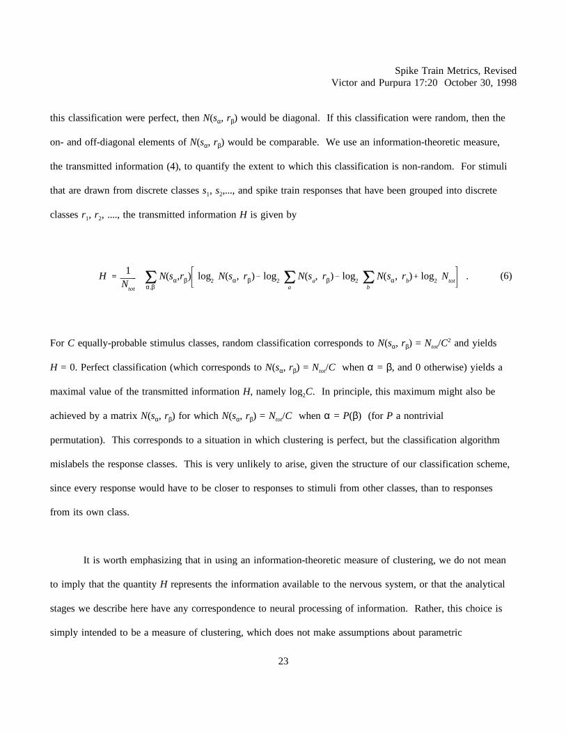
Spike Train Metrics, RevisedVictor and Purpura 17:20 October 30, 1998
this classification were perfect, then N(sα, rβ) would be diagonal. If this classification were random, then the
on- and off-diagonal elements of N(sα, rβ) would be comparable. We use an information-theoretic measure,
the transmitted information (4), to quantify the extent to which this classification is non-random. For stimuli
that are drawn from discrete classes s1, s2,..., and spike train responses that have been grouped into discrete
classes r1, r2, ...., the transmitted information H is given by
(6)H 1N
tot α,β
N(sα,rβ)
log2
N(sα, rβ) log2
a
N(sa, rβ) log
2 b
N(sα, rb) log
2N
tot .
For C equally-probable stimulus classes, random classification corresponds to N(sα, rβ) = Ntot/C2 and yields
H = 0. Perfect classification (which corresponds to N(sα, rβ) = Ntot/C when α = β, and 0 otherwise) yields a
maximal value of the transmitted information H, namely log2C. In principle, this maximum might also be
achieved by a matrix N(sα, rβ) for which N(sα, rβ) = Ntot/C when α = P(β) (for P a nontrivial
permutation). This corresponds to a situation in which clustering is perfect, but the classification algorithm
mislabels the response classes. This is very unlikely to arise, given the structure of our classification scheme,
since every response would have to be closer to responses to stimuli from other classes, than to responses
from its own class.
It is worth emphasizing that in using an information-theoretic measure of clustering, we do not mean
to imply that the quantity H represents the information available to the nervous system, or that the analytical
stages we describe here have any correspondence to neural processing of information. Rather, this choice is
simply intended to be a measure of clustering, which does not make assumptions about parametric
23
Spike Train Metrics, RevisedVictor and Purpura 17:20 October 30, 1998
relationships, if any, among the stimulus classes.
Biases due to small sample size. If the number of presentations of each stimulus class is small , then
the value of H estimated by eq. (6) will be spuriously high, simply because of chance proximities between the
few examples of observed responses. Even if there are a large number of stimulus presentations, one
anticipates an upward bias of the estimate of H. For example, in the case of C equally probable stimulus
classes, any deviation of N(sα, rβ) from the expected value of Ntot/C2 will result in a positi ve value of the
estimated transmitted information H. This problem represents a general diff iculty in the estimation of
transmitted information from limited samples (7).
Recently, Treves and Panzeri (45) have derived an analytic approximation to this bias: asymptotically,
the bias (for a fixed number of stimulus and response bins) is inversely proportional to the number of samples
and is independent of stimulus and response probabiliti es. The derivation of this asymptotic behavior
assumes that there is a binning process which treats all responses in an independent manner. The present
approach explicitl y avoids such a binning process, so there is no guarantee that a similar correction is
applicable. For this reason, we choose a computational approach to estimate this bias (9, 29): we use eq. (6)
to recalculate the transmitted information H following random reassignments of the observed responses S to
the stimulus classes. Values of the un-resampled H which lie in the upper tail of this distribution are thus
unlikely to represent a chance grouping of responses. Furthermore, the average value of many such
calculations, which we denote H0, is an estimate of the upward bias in the estimate of H.
Examples: simple simulations
24

Spike Train Metrics, RevisedVictor and Purpura 17:20 October 30, 1998
We now present some examples in which we apply the above procedures to some simple numerical
simulations. These numerical simulations are not intended to be realistic, but rather to ill ustrate some of the
behaviors described above.
Rate discrimination: regular and irregular trains. The first example (Figure 4) concerns stimuli which
elicit different mean rates of firing. We considered five stimulus classes, each of which elicited firing at
different average rates (R = 2, 4, 6, 8, and 10 impulses/sec). Twenty examples of one-second responses to
each stimulus were simulated, and the transmitted information was calculated from these Ntot= 100 spike
trains according to eq. (6). These calculations were repeated for forty independent synthetic datasets, to
determine the reliabilit y (± 2 s.e.m.) of these estimates of transmitted information H. For each of these forty
datasets, two resamplings by relabelli ng, as described above, was performed to estimate the contribution H0
due to chance clustering. These calculations were performed for values of q spaced by factors of 2, and for
four values of the clustering exponent z: -8, -2, 2, and 8. We focus on the behavior of Dspike; the behavior of
Dinterval was very similar (data not shown).
In Figure 4A-D, the spikes were distributed in a Poisson fashion (c.v. = 1.0) for each of the five firing
rates R. In this case, the precise time of occurrence of each spike carries no information. Indeed, more
clustering (higher H) is seen for Dcount (Dspike[0]) than for Dspike[q], for q > 0. For low values of q, the decrease
in H for q > 0 is relatively minor (from about 0.7 to 0.5 for negative z, and essentially no decrease for
positi ve z). In this range (q < 16), Dspike[q] is influenced by a mixture of spike counts and spike times. For
suff iciently high values of q, H fall s to chance levels. In this range (q > 32), the cost of moving a spike is
suff iciently high so that nearly all minimal paths correspond to deletion of all spikes followed by reinsertion at
25

Spike Train Metrics, RevisedVictor and Purpura 17:20 October 30, 1998
other times. Consequently, the defining feature of each stimulus class (i.e., a similar number of spikes) is
ignored, and responses within the same stimulus class, especially at high firing rates, are seen (by Dspike[q]) as
very different.
Figure 4E-H shows a similar calculation, but with a spike generating process that is more regular
(c.v. = 0.125). To simulate responses to a class characterized by a steady mean rate R, we selected every kth
spike from an underlying Poisson process with rate kR. (The first spike is chosen at random from the initial k
spikes of this underlying process). In this "iterated Poisson" process, the interspike intervals were distributed
according to a gamma distribution of order k:
p(t) 1Γ(k)
R k t k 1 e Rt ,
where p(t) is the frequency of interspike intervals of length t. In the simulations shown here, we chose
k = 64, and thus the interspike intervals have a coeff icient of variation of 0.125 (=1/√k). Because the spike
trains are regular, there is less variabilit y in the number of spikes in each sample. Consequently, the spike
count metric Dcount leads to a greater degree of clustering than in the Poisson case (Figure 4A-D) -- calculated
values of H are approximately 2.0, close to the maximum achievable value of log2(5) ≈ 2.32. Nevertheless,
for small values of q and negative values of z (Figure 4E-F), there is a further increase in H. This increase
reflects the fact that within a class, responses will be similar not only in the number of spikes: additionally,
responses whose first spikes occur at similar times will have subsequent spikes that occur at similar times.
That is, the optimal match between a response to a given stimulus and other responses in the same class will
26

Spike Train Metrics, RevisedVictor and Purpura 17:20 October 30, 1998
be stronger if spike times, and not just spike counts, are considered. However, there is an optimal choice for
q, beyond which further increases lead to decreasing values of H. This is because a cost q corresponds to the
notion that the timing of a spike matters up to an amount 1/q. Choosing q too high for the typical precision
of the spike times causes the distance measure to be influenced by details that are irrelevant to the response
classes. Consequently, for high q, the apparent clustering decreases.
Note that for positi ve z (Figure 4G-H), there is no increase in H for any value of q. This is because
the clustering based on the average distance as defined by eq. (5) now assigns each response to the class with
the "least bad" match, rather than the "most good" match. Sensiti vity to spike times improves the quality of
the best match, but worsens the quality of the worst match.
We also point out that, despite the fairly large dependences H on q and z seen in Figure 4, there is
relatively littl e dependence of H0, the estimate of chance information. That is, the increase in temporal
resolution associated with high q is not associated with large upward biases in estimates of information, as
would have been the case if increased temporal resolution were to require increasingly sparse sampling of a
space of progressively higher dimension.
This simulation shows that for response classes which differ in overall firing rate (and thus, are readily
discriminable by a simple rate code), metrics which are sensiti ve to temporal pattern allow enhanced
discrimination. This modest enhancement is restricted to regular spike trains (Figure 4E-H) and values of q
which are not so large as to regard even minor shifts of spike times as "different." For irregular trains, and
for high values of q, attention to temporal structure reduces discrimination, as would be expected since the
27

Spike Train Metrics, RevisedVictor and Purpura 17:20 October 30, 1998
temporal structure is irrelevant to the response classes.
Temporal phase discrimination. The next three examples present situations in which Dspike and Dinterval
have contrasting behavior. Figure 5 shows a simulation of temporal phase discrimination. There were four
stimulus classes, each with 20 simulated responses of 1 second duration. In Figure 5A-D, we used a time-
dependent Poisson process to generate spike trains. The instantaneous firing density R(T) was given by
R0[1 + m cos(2πfT + φ)], where the mean firing rate R0 was 20 impulses/sec, the modulation frequency f was 4
Hz, and the modulation depth m was 0.5. The stimulus classes differed in their modulation phase φ, which
was chosen from the set { 0, π/2, π, 3π/2} . Thus, responses to different stimulus classes were anticipated to
differ in the arrangement of spike times, and not in the average total number of spikes (or in the distribution
of the number of spikes). The information-theoretic index of clustering H, and the clustering H0 due to
chance alone, were calculated from 40 independent simulations, as in Figure 4. As is seen in Figure 5A-D,
clustering was at chance level for Dcount. In contrast, Dspike[q] revealed highly significant clustering. The peak
of H at q = 32 corresponds to 1/8 of a cycle (half the phase increment which separates the stimulus classes).
For substantiall y smaller values of q, clustering is diminished because the distinction between the classes is
diminished; for substantiall y larger values of q, clustering is diminished because the distance is influenced by
jitters in the spike times which are irrelevant to the response classes. This behavior was seen for all values of
the clustering exponent z.
Figure 5A-D also shows the degree of clustering revealed by Dinterval:fix[q] and Dinterval:min[q]. These
metrics, which are sensiti ve to the sequence of interspike intervals but not to the absolute time of occurrence
of spikes, reveal almost no clustering beyond chance. The two metrics differ only in how they treat the first
28

Spike Train Metrics, RevisedVictor and Purpura 17:20 October 30, 1998
and last interspike intervals (i.e., the time between the start of the response and the first spike, and the time
between the last spike and the end of the response period): Dinterval:fix[q]regards these intervals as fixed, while
Dinterval:min[q] adjusts them to minimize the distance. As such, Dinterval:fix[q] would be expected to retain a slight
sensiti vity to temporal phase, because it retains the first and last intervals. However, this only results in a
minimal (<0.05) increase in H.
In Figure 5E-H, the same instantaneous firing densities R(T) = R0[1 + m cos(2πfT + φ)] were used to
drive an iterated Poisson process of order k = 64. The resulting spike trains are much more regular (eightfold
decrease in the coeff icient of variation of the interspike interval), and clustering is much stronger.
Furthermore, the range of values of q for which Dspike shows significant clustering is substantiall y extended.
The range of effective values of q extends further downward because shifts in time of multiple adjacent spikes
are correlated. The range of effective values of q extends further upward (approximately by a factor of 8)
because of the proportionate decrease in the coeff icient of variation and the corresponding shortening of the
timescale at which precise timing becomes meaningless. Somewhat surprisingly, Dinterval:fix[q] and
Dinterval:min[q] also reveal significant clustering for these spike trains. This is an indirect consequence of the
regularity of the interspike intervals. One candidate path of elementary steps between responses from different
stimulus classes will consist of deleting some interspike intervals from the beginning of one response, deleting
some interspike intervals from the end of the other response, and stretching the intervening intervals to
achieve a match. This kind of path will reveal phase-dependent clustering. However, whether this path is
optimal (and hence, whether its total cost determines the distance) depends on the tightness of the match
between interspike intervals, and thus, on regularity of the spike trains. Dinterval:fix[q] has an advantage over
Dinterval:min[q] because of the end-effect discussed above provides independent absolute phase information, but
29

Spike Train Metrics, RevisedVictor and Purpura 17:20 October 30, 1998
this advantage is slight. All of these findings are largely independent of the choice of the clustering exponent
z.
In sum, this simulation shows that Dspike, but not Dcount or Dinterval, can discriminate among irregular
spike trains which vary in temporal phase (Figure 5A-D). For regular spike trains with instantaneous firing
frequencies, both Dinterval and Dspike can perform the discrimination (Figure 5E-H).
Temporal frequency discrimination. In this simulation (Figure 6), there were four stimulus classes,
each with 20 simulated responses of 1 second duration, and an instantaneous firing density R(t) was given by
R0[1 + m cos(2πft + φ)], with a mean firing rate R0 of 20 impulses/sec. For three of the classes, the
modulation depth m was 0.5, and the phase φ was chosen at random in each trial. These classes were
characterized by the modulation frequency f, which was chosen from the set { 3, 4, 5} . The fourth class was
unmodulated (m = 0, f and φ irrelevant). Thus, responses to different stimulus classes were anticipated to
differ primarily in the arrangement of interspike intervals (because they differed in modulation frequency), but
not in absolute spike times (since the initial phase φ was chosen at random). The information-theoretic index
of clustering H, and the clustering H0 due to chance alone, were calculated as in Figure 4 and Figure 5. For
spike times generated by a time-dependent Poisson process (Figure 6A-D), there is essentially no stimulus-
dependent clustering for any of the metrics considered. This is because the irregularities of the interspike
interval distributions due to the random times of occurrence of the spikes dominate the systematic temporal
modulation. However, for spike times generated by the more regular iterated Poisson process (Figure 6E-H),
substantial stimulus-dependent clustering is seen. We first consider Dinterval:fix[q] and Dinterval:min[q]. There are
two regimes: for q greater than 0 but no greater than 8, clustering is substantiall y greater than chance, but not
30
Spike Train Metrics, RevisedVictor and Purpura 17:20 October 30, 1998
suff iciently great to reliably distinguish the four classes from one another. In this range, the degree of
clustering depends strongly on the clustering exponent z (increasing as z decreases), indicating that it reflects
the presence of a few good matches rather than the absence of bad matches. For larger values of q, the
degree of clustering approaches the maximal possible value of log2(4) = 2. The height and position of this
peak (though not its breadth) are relatively independent of z. Dinterval:min[q] has a slight advantage over
Dinterval:fix[q], corresponding to the fact that it ignores the initial and final interspike intervals, which are
irrelevant to the distinction between the classes. Note that although these stimulus classes were constructed to
be distinguished on the basis of spike intervals, rather than spike times, Dspike[q] nevertheless reveals
significant clustering. This is analogous to the behavior of Dinterval:fix[q] and Dinterval:min[q] in phase
discrimination (Figure 5E-H). However, clustering in the sense of Dspike[q] is sensiti ve to z because good
matches at one relative phase will necessaril y imply bad matches at other relative phases. Thus, average
distances (as defined by eq. (5)) that are weighted heavily by the best match (i.e., z < 0) will t end to reveal
the greatest degree of clustering.
Identification of deterministic chaos. In the next simulation (Figure 7), the two response classes are
distinguished by the presence or absence of deterministic chaos (loosely inspired by observations of low-
dimensional chaos in the olfactory system (41)). In both stimulus classes, responses consisted of impulse
trains in which the interspike intervals were uniformly distributed between 0 and 2/R0, with the mean rate R0,
set at 10 impulses/sec. For spike trains in the first class, these interspike intervals were placed in random
order. For spike trains in the second class, the first interspike interval is chosen at random, but subsequent
interspike In+1 intervals are determined from the preceding interval In by the Baker transformation,
31

Spike Train Metrics, RevisedVictor and Purpura 17:20 October 30, 1998
(8)
2 In , In ≤ 1R0
In 1
.
2 ( 2R
0
In
) , In
> 1R
0
For each calculation of H, 100 1-second examples of each response were generated. H and H0, and|
their s.e.m.'s, were estimated as in the previous simulations from 20 independent simulations. These spike
trains had identical distributions of interspike intervals, identical mean rates (R0 = 10 impulses/sec), flat post-|
stimulus time histograms, and no pairwise correlations between intervals at second order. Thus, in contrast to
the previous simulations (Figure 4, Figure 5, and Figure 6), traditional approaches such as Fourier analysis, as
well as some more recently-proposed ideas (13, 26) would not have been able to distinguish these response
classes.
As seen in Figure 7, substantial clustering beyond that expected from chance alone is seen for all three
metrics considered. The advantage of Dinterval:min[q] and Dinterval:fix [q] over Dspike[q] makes sense, because of the
interval-based nature of the temporal structure. Interestingly (Figure 7A-B), in contrast to the previous
simulations, some estimates of H continue to rise for high values of q. This is because successive iterations of
the transformation (eq. (8)) are sensiti ve to indefinitely small changes in interspike interval lengths, as is
characteristic of chaotic processes in general. Thus, sensiti vity to tiny changes in interval length improves the
quality of mutual matches among samples of the chaotic process. This behavior is not seen for Dspike[q]
32

Spike Train Metrics, RevisedVictor and Purpura 17:20 October 30, 1998
(which is only indirectly sensiti ve to interval length), nor for positi ve values of z (where clustering is weighted
by the absence of mismatches, rather than by the closeness of the best match).
The geometries induced by a family of metrics
We now return to a simple rate-discrimination simulation to ill ustrate the way that changes in the
metric induce changes in the nature of clustering. We consider two stimulus classes, which elicit responses of
mean rates 6 and 7 impulses/sec respectively and have interspike intervals determined by an iterated Poisson
process of order k = 64. For this simulation, 40 example spike trains for each class were simulated, and the
information-theoretic measure of clustering, H, was calculated for Dspike[q] for a range of values of q and a
clustering exponent z = -2. The dependence of H on q (Figure 8) was similar to that seen in Figure 4E-H: a
modest increase in clustering for q > 0, followed by an abrupt fall -off f or values of q suff iciently high as to
force sensiti vity to irrelevant detail i n the spike trains. However, despite the modest change in H, there is a
qualitative change in the nature of the clustering for low values of q (e.g., q = 1), and values of q near the
peak in H (e.g., q = 16). To see this, we use multidimensional scaling (16, 20) to embed the spike trains into
a Euclidean space. This procedure assigns coordinate n-tuples to each spike train, so that the standard
Euclidean distances between these n-tuples are as close as possible to the distances yielded by a given metric,
in this case Dspike[q]. Successive coordinates correspond to eigenvectors of a symmetric matrix Mjk, scaled by|
the square roots of the corresponding eigenvalues. The entries of the matrix Mjk are given by|
|
(9)
33

Spike Train Metrics, RevisedVictor and Purpura 17:20 October 30, 1998
|
where Djk indicates the distance between spike train j and spike train k, < >r indicates an average over all
spike trains r, < >s indicates an average over all spike trains s, and < >rs indicates an average over all pairs
of spike trains r and s. Note that this embedding does not guarantee that all points in the Euclidean space
correspond to spike trains -- merely that the distances of spike trains, in the sense of Dspike[q], are well -
approximated by the Euclidean distances between their n-tuples. Additionally, the matrix of eq. (9) may have
negative eigenvalues, corresponding to a hyperbolic geometry in the embedding space. Nevertheless, the
embedding provides a visual way to understand the geometry induced by the metrics Dspike[q].
The multidimensional scaling procedure was applied to each response class (40 samples) in isolation,
as well as to the combined dataset of 80 samples. Figure 9A shows the results for q = 1. Consider first the
multidimensional scaling of the "6 imp/sec" class in isolation (left inset). For q = 1, Dspike[q] is determined
primarily by the number of spikes. Most spike trains in the "6 imp/sec" class have 6 spikes, but some have 5
spikes, and some have 7 spikes. Hence, the spike trains form three clouds, arrayed approximately in a line,
one corresponding to each spike count. Spike trains with the same number of spikes are close to each other
but not identical. This is reflected in the dispersion of the points within each cloud and the requirement for
more than one dimension to account fully for the distances determined by Dspike. A similar picture is seen for
the multidimensional scaling of the "7 imp/sec" class in isolation (right inset). Combined multidimensional
scaling (main scattergram) of the two classes yields four clouds, corresponding to the four possible spike
counts of 5, 6, 7, and 8 impulses. Only the "6 imp/sec" class contributes to the cluster corresponding to 5
impulses (the three left-most clusters), and only the "7 imp/sec" class contributes to the cluster corresponding
to 8 impulses (the three right-most clusters), and both stimulus classes contribute to the clusters with 6 and 7
34
Spike Train Metrics, RevisedVictor and Purpura 17:20 October 30, 1998
impulses. This overlap corresponds to the imperfect discrimination of these two classes by clustering based
on Dspike[1]. The scatter along the second dimension does not help to disambiguate these responses.
Figure 9B shows the corresponding picture for q = 16. Dspike[16] is sensiti ve to times on the order of
0.1 sec, and on this scale, both spike trains are quite regular (mean intervals of 0.166 and 0.143 sec, with c.v.
of 0.125). The locus corresponding to the "6 imp/sec" class in isolation (left inset) now forms an
approximate circle. This corresponds to the fact that for Dspike[16], the distance between two fairly regular
spike trains is determined primarily by their relative phase. Multidimensional scaling of the "7 imp/sec" class
in isolation gives a similar picture (right inset). Note that there are no points at the center of either ring: such
points would correspond to spike trains which are not only equidistant from all of the spike trains, but also
close to all of them; such spike trains (in the context of Dspike[16]) do not exist. Multidimensional scaling of
the combined classes requires four dimensions -- the first four eigenvalues of the matrix of eq. (9) are 0.348,
0.284, 0.240, and 0.208. In the two-dimensional projection ill ustrated (main scattergram), the points
corresponding to the two stimulus classes appear to form interpenetrating clouds. Examination of the higher-
dimensional representation reveals that these clouds correspond, approximately, to two mutually orthogonal
circles, one corresponding to each class. That is, within each class, the spike trains' locus is approximately
circular, and all points in one class are, approximately, at the same distance from all points in the other class.
In contrast to the situation for q = 1, multiple dimensions contribute to separation of the response classes.
Furthermore, the geometrical center of the two response classes is similar -- near the origin -- and hence, a
clustering scheme which assumed that the responses lay in convex clouds would have failed.
Yet a third kind of behavior is seen for Dspike[256]. This distance is sensiti ve to times on the order of
35

Spike Train Metrics, RevisedVictor and Purpura 17:20 October 30, 1998
0.01 sec. On this timescale, both classes of spike trains are irregular. Consequently (Figure 9C), no
discernable geometrical structure is apparent in the multidimensional scaling of the spike trains in isolation
(left and right insets): they form what appears to be a random cloud. Multidimensional scaling of the
combined classes again forms a random cloud (main scattergram), either when inspected in the projection
ill ustrated, or in projections along higher-order eigenvectors. This corresponds to the fact that this metric is
sensiti ve to differences between individual responses (idiosyncratic timing of spikes) which are unrelated to
differences between the stimulus classes.
These three regimes are summarized by the analysis of Figure 10. We introduce a dimension index E,
which describes the effective dimension of an embedding. The dimension index E is defined by
where λi are the eigenvalues of the matrix of eq. (9). Note that for an embedding in which each of n
(10)
dimensions contributed equally (λi = 1/n), this index would have the value n. For q in the range 4 to 32, the
dimension index for the embedding of each class in isolation is approximately 2 (light and dark symbols), and
the dimension index for the combined classes is approximately 4 (solid line without symbols). This
corresponds to a circular locus for each of the classes in isolation, and bi-orthogonal circles for the embedding
of the combined classes (Figure 9B). For lower values of q, the effective dimension decreases towards 1, and
the dimension index for the embedding of the combined classes is no larger than that of the classes in
isolation. That is, the higher dimensions do not contribute to stimulus-dependent clustering. For values of
q > 32, the dimension index rises rapidly, but, as we have seen in Figure 9C, this increase in dimension does
not produce any discernable structure. It should be noted that one can always achieve an embedding of n|
36
Spike Train Metrics, RevisedVictor and Purpura 17:20 October 30, 1998
points in a space of dimension n-1 (39 and 79 in the present case), and thus (for q > 128) it is li kely that our|
estimates of dimension in Figure 10 are lower bounds, limited by the number of spike trains we chose to|
generate.
However, it is not the case that a progressive increase in embedding dimension necessaril y implies a
decrease in clustering. Indeed, the opposite situation is seen for the discrimination of deterministic chaos and
randomly-sequenced interspike intervals. Figure 11 shows the dependence of the dimension index E (eq.
(10)) on q for embeddings of the chaotic spike trains in isolation, the random spike trains in isolation, and the
two classes combined. For all three families of metrics (Figure 11A: Dspike; Figure 11B: Dinterval:fix; Figure 11C:
Dinterval:min), the set of chaotic spike trains is associated with a lower embedding dimension than the random
trains, and this dimension increases monotonically with q. In contrast to the simple geometrical situation of
the regular spike trains (Figure 9C), the rise in dimension is not associated with a decrease in clustering --
rather, as we have seen in Figure 7, clustering continues to rise with increasing q. It is also worthwhile to
note that the high embedding dimension is not associated with an increase in the chance clustering (dashed
lines in Figure 7). This suggests that our purely metrical approach to clustering has successfully circumvented
the problem of attempting to perform clustering in a sparsely-populated high-dimensional vector space, which
would be anticipated to lead to progressively higher estimates of chance clustering with increasing
dimensionality.
Comparison with a benchmark set of simulated data
The final simulation utili zes a benchmark dataset, developed by Golomb et al. (14) to compare a
37
Spike Train Metrics, RevisedVictor and Purpura 17:20 October 30, 1998
variety of methods to determine the information content of spike trains. These simulations (15) generate
responses of idealized lateral geniculate magnocellular and parvocellular neurons to spatial patterns consisting
of Walsh functions. The responses to each Walsh pattern are derived from a time-dependent Poisson process,
whose envelope is determined by convolving the Walsh pattern with modelled spatiotemporal filtering
properties of lateral geniculate neurons. For the simulations of Figure 12A and B, datasets are constructed
from 64 responses (250 msec in duration) to each of the 32 patterns, and the above procedures are used to
calculate information-theoretic measures of clustering H for Dspike[q] and Dinterval:min[q]. H0 is determined by
repeating this calculation for 5 random reassignments of the responses to stimuli . This procedure is repeated
for 16 independent datasets of 64 responses per pattern.
As seen in Figure 12A and B, the estimate of chance clustering, H0, is substantiall y larger than in the
simulations discussed previously, as one would expect from the fact that there is a relatively small ratio of
samples to classes (7, 45). For the modelled magnocellular neuron (Figure 12A), clustering is maximal for
Dspike[q] with qmax = 32. The increase in H for Dspike[32] compared to Dcount = Dspike[0] exceeds the
corresponding change in H0. That is, the measure of clustering corrected for the bias due to small sample
size, H - H0, is largest for Dspike[32]. For q < 128, clustering for Dspike exceeds clustering for Dinterval:min,
whether or not the correction term H0 is subtracted. Thus, for the magnocellular neuron of this simulation, the
timing of impulses (to within a precision of ca. 1/qmax = 30 msec) conveys significant stimulus-dependent
information. For the modelled parvocellular neuron (Figure 12B), the situation is quite different. There is
only a modest increase in H for q > 0, and this increase is less than the increase in H0. That is, H - H0 is
largest for Dcount; there is no evidence for improvement in clustering either for Dspike or Dinterval:min.
38
Spike Train Metrics, RevisedVictor and Purpura 17:20 October 30, 1998
Figure 12C and D show how this analysis depends on the number of samples per stimulus class. As
the number of samples increases, H and H0 decrease. For each metric considered, these decreases are
approximately parallel, and consequently, the corrected estimator of clustering, H - H0. changes by a relatively
small amount. (Nevertheless, it is notable that this drift is upward, which suggests that subtraction of H0 may
be an overly conservative correction.) For the modelled magnocellular neuron (Figure 12C), H - H0. is largest
for Dspike provided that there are at least 32 samples per stimulus class. For the modelled parvocellular
neuron (Figure 12D), H - H0. is largest for Dcount for all values of the number of samples per stimulus class.
It is interesting to compare our empirical estimates of H0. with the analytic result of Treves and
Panzeri (45). Consistent with this result, there is an approximate inverse proportionality between H0 (dashed
lines in Figure 12C and D) and the number of samples per stimulus class. However, this proportionality
constant is dependent on the metric and also (dashed lines in Figure 12A and B) on the value of q. This
appears to be at variance with the analytic result (45), which states that asymptotically, this proportionality
constant depends only on the size of the stimulus and response classes, and the number of samples. However,
there is no contradiction: Treves and Panzeri's derivation (45) requires that the assignments of samples to
response categories be made independently. Independence is violated by the clustering scheme we used, and
the consequent dependence of the proportionality constant on the metric that we observe emphasizes the
necessity of the assumption of independence for the analytic result (45).
The estimates in Figure 12C and D of H and H - H0 may be compared directly with the calculations
of Golomb and coworkers (14) for these simulated datasets, based on a binning approach and on neural
network classifiers (19). For the magnocellular neuron, our estimate of H - H0 for Dcount (0.19 for 128
39

Spike Train Metrics, RevisedVictor and Purpura 17:20 October 30, 1998
samples/class) approximated the estimates obtained by Golomb et al. (14) (≈ 0.24 for 128 samples/class for
binning or for network classifiers) for the "number of spikes" code. We found an increase in H - H0 to 0.34
for Dspike, while Golomb et al. (14) found an increase (to ≈ 0.5 for the binning method, ≈ 0.4 for the neural
network classifier method) for multidimensional codes based on three principal components. For the
parvocellular neuron, our estimate of H - H0 for Dcount (0.81 for 128 samples/class) approximated the estimates
obtained by Golomb et al. (14) (≈ 0.85 for 128 samples/class for binning or neural network classifiers) for the
"number of spikes" code. We found no increase in H - H0 for Dspike or Dinterval:min; Golomb et al. (14) found a
slight increase (≈ 0.95 for binning or neural network classifiers) for multidimensional codes based on three
principal components.
Some neurophysiological examples
In Figure 13, we re-analyze data recently published by Middlebrooks et al. (28) as evidence for
temporal encoding of the azimuth of an auditory stimulus. The spike trains were recorded from a single
neuron in cat anterior ectosylvian cortex following noise bursts of 100 msec duration which were presented in
20 deg steps of azimuth in the horizontal plane. For the analysis presented here, the 10 responses to each of
these 18 locations were rebinned into sets of 30 responses corresponding to 60 deg sectors. Figure 13A shows
the information-theoretic measure of clustering, H, for Dspike and Dinterval:min, along with values of H0 as
calculated from 10 random permutations of the data. There is a clear rise in H for q > 0, both for Dspike and
Dinterval:min. The increase for Dinterval:min seems somewhat greater than for Dspike , but there is a similar difference
in the correction term H0. Additionally, there is a sharp peak in Dspike[q] near q = 256, which is not associated
with an increase in the correction term H0. This indicates that spike times, up to a precision of 1/q ≈ 4 msec,
40

Spike Train Metrics, RevisedVictor and Purpura 17:20 October 30, 1998
cluster in a stimulus-dependent fashion. (Note that the ±2 s. e. m. lines in Figure 13A represent are
confidence limits for the mean of H0, and thus are only appropriate for comparison among different resampled
estimates. To estimate the probabilit y that the un-resampled value of H could have come from this
population, a ±2 standard deviation criterion (√10 ≈ 3.2 times the s. e. m) should be used; by this measure,
H is significant for all values of q.)
In Figure 13C and D, we present the results of multidimensional scaling of these responses, with the
distance function provided by Dspike[256]. Figure 13C shows the loci which correspond to individual responses,
as projected into the plane of the first two eigenvalues. There is certainly substantial overlap of the clouds
corresponding to each azimuth range, but nevertheless, a trend towards segregation of responses from each
sector is apparent. This trend is made much more vivid in Figure 13D, which shows only the geometrical
center of each cloud. The dimension index E (eq. (10)) of this embedding is 2.8, and the first 10 eigenvalues
are shown in Figure 13B. The first four eigenvalues are positi ve, but projections of the loci of the spike trains
on the third and fourth axes do not reveal additional geometrical structure.
In Figure 14, we analyze a dataset obtained in our study (47) of temporal coding in macaque visual
cortex. The data consist of activity recorded in primary visual cortex in an awake animal performing a fixation
task. Stimuli consisted of transient presentation of gratings of five spatial frequencies (1, 3, 5, 11, and 21
c/deg), aligned in each of 8 orientations (0 deg to 157.5 deg in 22.5 deg steps), at a contrast of 1.0 (Here,
contrast is defined as [(Lmax - Lmin)/(Lmax + Lmin)], where Lmax and Lmin are the maximum and minimum of the
stimulus luminance.) For each of these 5 x 8 = 40 stimuli , 16 responses of 256 msec were collected and
analyzed. As seen in Figure 14A, there is temporal coding both in the sense of Dspike[q] and Dinterval:min[q], as
41

Spike Train Metrics, RevisedVictor and Purpura 17:20 October 30, 1998
shown by the rise in H for q > 0. However, there is a falloff in H by q ≈ 50, indicating a much looser jitter of
1/q ≈ 20 msec for the temporal structure in this neuron's encoding in comparison with the auditory neuron of
Figure 13. Multidimensional scaling of the responses according to the metric Dspike[32] requires at least three
dimensions to reveal the geometrical structure of the response loci (Figure 14C, D, and E). For each of the
four lowest spatial frequencies, the responses to different orientations form a loop, and these loops are largely
non-overlapping when examined in three dimensions. For example, the orbits for spatial frequencies 3 and 4
overlap in dimensions 1 and 2, but are well -separated in dimension 3. Conversely, the orbit for spatial
frequency 1 nearly collapses in dimensions 1 and 3, but is clearly delineated along dimension 2. The
dimension index E (eq. (10)) of this embedding is 1.8, and the first 10 eigenvalues are shown in Figure 14B.
Projections along combinations of the third and fourth axes provide additional separation of the orbits, but do
not reveal qualitatively new structure.
In Figure 15, we analyze activity of a complex cell i n the supragranular layers of primary visual
cortex, recorded in an anaesthetized, paralyzed macaque. (Physiological preparation for recordings in the
anaesthetized, paralyzed macaque are described in (48)). Stimuli consisted of transient presentation of
gratings of three spatial frequencies (0.5, 2, and 4 c/deg) and five contrasts (0.0625, 0.125, 0.25, 0.5, 1.0),
aligned at the optimal orientation. For each of these 3 x 5 = 15 stimuli , 128 responses of 256 msec were|
collected and analyzed. Again there is temporal coding both in the sense of Dspike[q] and Dinterval:min[q], as
shown by the rise in H for q > 0. As in data of Figure 14, multidimensional scaling of the responses
(Figure 15C, D, E) for Dspike[64] reveals a systematic separation of the loci for each of the three spatial
frequencies and the five contrasts, but three dimensions are needed to see this separation clearly. Responses
to the lowest spatial frequency are well -separated from the responses to the two higher spatial frequencies in
42

Spike Train Metrics, RevisedVictor and Purpura 17:20 October 30, 1998
the projection on dimensions 1 and 2, while responses to the two higher spatial frequencies are best separated
from each other in the projection on dimensions 1 and 3.
In contrast to the data of Figure 14, clustering is greater for Dinterval:min[q] than for Dspike[q] at large
values of q. However, multidimensional scaling (Figure 16B, C, D) for Dinterval:min[64], the same value of q as
in Figure 15, does not provide a systematic separation of the loci for each of the three spatial frequencies.
Rather, the loci for all stimuli are nearly colli near, and the loci for the two higher spatial frequencies overlap
in all projections. This qualitatively simpler structure for the geometry induced by Dinterval:min[q] is made
quantitative by the greater dominance of the first eigenvalue (Figure 16A compared with in Figure 15B), and
the smaller dimension index E (1.6 for Dinterval:min[64], compared with 3.7 for Dspike[64]). That is, even though
Dinterval:min[64] provides a greater degree of clustering than Dspike[64], Dspike[64] induces a metrical structure
which separates the two stimulus attributes of contrast and spatial frequency, while Dinterval:min[64] does not.
43

Spike Train Metrics, RevisedVictor and Purpura 17:20 October 30, 1998
DISCUSSION
Overview
We have presented a new approach to the analysis of the temporal structure of spike trains. The
notion of "distance" between spike trains plays a central role in this approach. Based solely on the notion of
distance, we show how it is possible to assess (via an information-theoretic measure) the extent to which
experimentally-measured neural responses cluster in a systematic fashion. This measure of clustering indicates
to what extent this candidate distance is sensiti ve to features of spike trains that convey stimulus-specific
information. By repeating this process for several families of distances, one can learn about the nature and
precision of temporal coding.
The notions of distance make explicit and fundamental use of the point-process nature of spike trains.
The formal structure of this approach is an embedding of spike trains into a "metric space." Metric spaces
have well -defined distances but do not require the assumption of a linear structure (with implications for
superposition and scaling) that would be inherent had we embedded spike trains into a vector space. As
pointed out recently by Hopfield (18), there are good theoretical reasons to question whether such vector-space
assumptions are appropriate. Indeed, the metrics we consider, which follow naturally from neurobiological
heuristics, are inconsistent with a linear structure. While one can use vector-space embeddings to visualize
the metrical relationships between spike trains (Figure 9, Figure 14D - E, Figure 15C - E, Figure 16B - D),
the high dimensionality and presence of hyperbolic coordinates in these embeddings indicates that the vector
space approximation is a poor one.
44

Spike Train Metrics, RevisedVictor and Purpura 17:20 October 30, 1998
This approach is fundamentally hypothesis-driven and in principle can be applied to any proposal for
temporal coding, provided that it can be formalized in terms of a metric, or a family of metrics that depends
on a parameter (such as our cost q). Comparison of clustering across distinct families of metrics provides
qualitative insight into the nature of coding, while comparison of clustering within a parametric family
provides quantitative insight (such as the "precision" of coding). We cannot prove that this approach will
encompass any notion of temporal coding ("encoding" as defined by Theunissen and Mill er (44)), but,
arguably, the notion of a metric is a sine qua non of any rigorous hypothesis for temporal coding. Certainly,|
this approach is at least as general as are methods that require vector-space embedding, since any such|
embedding automatically provides a metric (the Euclidean distance).
The metrics we have considered induce distinct topologies on the space of spike trains. Some of the
metrics we consider are related by a strict topological hierarchy (Figure 1). Indeed, adding a new kind of step
to the definition of a metric always leads to a metric which is coarser than (i.e., refined by) the original
metric. However, as the simulations and the analyses of experimental data show, topological refinement does
not necessaril y imply greater clustering. Moreover, parametric changes in the metric (i.e., variations in q)
result in no change in the induced topology but frequently in a dramatic change in the degree of clustering.
Bialek's reconstruction method (5) rests on a search for a function L(t) that, when convolved with a
spike train, provides an optimal reconstruction of a temporal input. Each candidate function L(t) defines a
distance (a Euclidean distance of spike trains convolved with L(t)), and the reconstruction approach can be
viewed as a minimization of such a distance. Except for "pathological" cases, the distances corresponding to
45

Spike Train Metrics, RevisedVictor and Purpura 17:20 October 30, 1998
each choice for L(t) have equivalent topologies (which are also equivalent to the one induced by Dspike). Thus,
in both approaches, the characterization of a temporal code appears to require more than merely the topology
induced by a metric.
Variety of behaviors revealed by this approach
For the two families of metrics we focussed on (Dspike and Dinterval), our methods readily reveal a
variety of behaviors in simulated datasets. This ranges from no (Figure 4A - D, Figure 6A - D) or minimal
(Figure 4E - F) evidence of temporal coding, to dramatic encoding by spike times and intervals
(Figure 5E - H), to encoding primarily by spike times and not by intervals (Figure 5A - D), to encoding
primarily by intervals and not by spike times (Figure 6E - H, Figure 7). Figure 7 also demonstrates that the
present approach, without further machinery, suff ices to identify coding through the genesis of deterministic
chaos. These qualitative behaviors are largely independent of the exponent z used for clustering.
In all of the analyses, the estimate of chance clustering H0 is relatively insensiti ve to the parameter of
temporal precision, q. This underscores the point that the temporal resolution of the analysis is achieved
without binning, and hence without an artifactual increase in apparent information despite the increase in
embedding dimension at high values of q (Figure 11). This is of particular practical importance given the
milli second precision (23, 24) that cortical neurons possess. The present approach provides a practical way to
determine whether spike times, at this level of precision, carry information concerning the stimulus, and thus
to differentiate between intrinsic precision and informative precision. The large optimal value of q for auditory
data (Figure 13) indicates a role for this high degree of temporal precision in this sensory modality. However,
46

Spike Train Metrics, RevisedVictor and Purpura 17:20 October 30, 1998
our analysis also indicates that this is not universal: for neurons in visual cortex, maximal clustering is
achieved for values of q that correspond to temporal precisions on the order of 20 msec (Figure 14, Figure 15)
or more (47), in agreement with measures of temporal precision achieved through more traditional analyses of
temporal coding (17).
Comparison with other clustering methods of analysis of temporal coding
Middlebrooks et al. (28) used a neural network approach to cluster spike trains and to demonstrate|
temporal coding of the azimuth of a sound's origin in the responses of single neurons in auditory cortex. Our|
finding of an increase in H for q > 0 (Figure 13A) is in agreement with the authors' inference (28) of temporal
coding, but we believe that our approach adds to the neural-network analysis carried out by the authors in
several ways. The peak in H near q ≈ 256 provides an estimate of 3 - 4 msec for the jitter of the temporal
structure. Comparison of the difference H - H0 for both Dspike[q] and Dinterval:min[q] shows that the pattern of
absolute spike times, but not of spike intervals, is systematically dependent on the stimulus. Finally,|
multidimensional scaling (Figure 13C and D) of the neural responses according to the distances Dspike[q] that|
are associated with strong clustering provides a vivid demonstration of the representation of the azimuth of a|
sound's origin in the temporal structure of the neural response.|
In comparison with the information analyses of temporal coding considered by Golomb et al. (14), the
present approach yields lower values of H and H - H0 by 0.05 - 0.1 (up to 20%). Presumably, this is a
consequence of two features of our approach: (i) We used a clustering method which made no assumptions
about the shapes of clusters. This has the advantage of identifying clusters even for spike train loci that are
47

Spike Train Metrics, RevisedVictor and Purpura 17:20 October 30, 1998
concentric (Figure 6, Figure 9), but it would li kely provide a less-eff icient clustering scheme in situations in
which spike train loci conformed to relatively uniform clouds. (ii ) The clustering was based on metrics Dspike
and Dinterval:min, which were chosen to test specific hypotheses concerning the nature of temporal coding, rather
than attempting to optimize them to separate spike trains which were created from time-dependent Poisson
processes.
Despite these differences, there is a substantial similarity in the biological conclusions that one would
draw from the two calculations: the greater information in the parvocellular neuron's responses, and the
greater relative importance of temporal coding in the magnocellular neuron's responses. This is reassuring for
potential users of either approach. The somewhat smaller value of H and H - H0 that we obtain is a
combination of the price paid for a more generic clustering algorithm and the deviation of the metrics Dspike
and Dinterval:min from the geometry that underlies the fundamentally linear simulation. That is, the difference in
apparent clustering is a window on the underlying geometry of the simulated spike trains themselves. It
remains to be seen whether a similar difference is generally found in the analysis of real neuronal discharges.
48

Spike Train Metrics, RevisedVictor and Purpura 17:20 October 30, 1998
ACKNOWLEDGEMENTS
The authors thank Peter Sellers for his insights and helpful discussions. A portion of this work was
presented at the 1994 meeting of the Society for Neuroscience, Miami (46). This work was supported by NIH
grants EY9314 (JDV) and NS01677 (KPP), The McDonnell -Pew Foundation (KPP), The Revson Foundation
(KPP), and The Hirschl Trust (JDV). We thank Mary Conte for her expert technical assistance, Chiye Aoki
and Teresa Milner for advice and assistance with histology, and Danny Reich for his comments on the
manuscript.
49

Spike Train Metrics, RevisedVictor and Purpura 17:20 October 30, 1998
BIBLIOGRAPHY
1. Abeles, M. (1982) Local Cortical Circuits, an Electrophysiological Study. Springer, Berlin.
2. Abeles, M. (1982) Role of the cortical neuron: integrator or coincidence detector? Isr. J. Med. Sci. 18,
83-92.
3. Abeles, M., & Gerstein, G.L. (1988) Detecting spatiotemporal firing patterns among simultaneously
recorded single neurons. J. Neurophysiol. 60, 909-924.
4. Abramson, N. (1963) Information Theory and Coding. McGraw-Hill , New York.
5. Bialek, W., Rieke, F., de Ruyter van Steveninck, R.R., & Warland, D. (1991) Reading a neural code.
Science 252, 1854 - 1857.
6. Bliss, T.V.P. & Colli ngridge, G.L. (1993) A synaptic model of memory: long-term potentiation in the
hippocampus. Nature 361, 31-39.
7. Carlton, A.G. (1969) On the bias of information estimates. Psychological Bulletin 71, 108-109.
8. Chee-Orts, M-N., & Optican, L.M. (1993) Cluster method for analysis of transmitted information in
multivariate neuronal data. Biol. Cybern. 69, 29-35.
9. Fagen, R.M. (1978) Information measures: statistical confidence limits and inference. J. Theor. Biol. 73,
61-79.
10. Fukunaga, K. (1990) Introduction to Statistical Pattern Recognition, 2nd ed. Academic Press, NY. 591 pp.
11. Gaal, S.A. (1964). Point Set Topology. Academic Press, NY. 317 pp.
12. Gawne, T.J., McClurkin, J.W., Richmond, B.J. , & Optican, L.M. (1991) Lateral geniculate neurons in
behaving primates. III . Response predictions of a channel model with multiple spatial-to-temporal filters. J.
Neurophysiol. 66, 809-823.
13. Geisler, W.S., Albrecht, D.G., Salvi, R.J., & Saunders, S.S. (1991) Discrimination performance of single
50

Spike Train Metrics, RevisedVictor and Purpura 17:20 October 30, 1998
neurons: rate and temporal-pattern information. J. Neurophysiol. 66, 334-362.
14. Golomb, D., Hertz, J., Panzeri, S., Richmond, B., & Treves, A. (1996) How well can we estimate the
information carried in neuronal responses from limited samples? Neural Computation, in press.
15. Golomb, D., Kleinfeld, D., Reid, R.C., Shapley, R.M., & Shraiman, B.I. (1994) On temporal codes and
the spatiotemporal response of neurons in the lateral geniculate nucleus. J. Neurophysiol. 72, 2990-3003.
16. Green, P.E. (1978) Analyzing Multivariate Data. Dryden Press, Hinsdale, IL. 519 pp.
17. Heller, J., Hertz, J.A., Kjaer, T.W., & Richmond, B.J. (1995) Information flow and temporal coding in
primate pattern vision. J. Computational Neuroscience 2, 175-193.
18. Hopfield, J. J. (1995) Pattern recognition computation using action potential timing for stimulus
representation. Nature 376, 33 - 36.
19. Kjaer, T.W., Hertz, J.A., & Richmond, B. J. (1994) Decoding cortical neuronal signals: network models,
information estimation, and spatial tuning. J. Computational Neuroscience 1, 109-139.
20. Kruskal, J.B., & Wish, M. (1978) Multidimensional Scaling. Sage Publications, Beverly Hill s. 93 pp.
21. Larson, J., Wong, D. & Lynch, G. (1986) Patterned stimulation at the theta frequency is optimal for the
induction of hippocampal long-term potentiation. Brain Res. 368, 347-350.
22. Laurent, G., Wehr, M., & Davidowitz, H. (1996) Temporal representations of odors in an olfactory
network. J. Neurosci. 16, 3837-3847.
23. Lestienne, R. (1996) Determination of the precision of spike timing in the visual cortex of anaesthetised
cats. Biol Cybern. 74, 55-61.
24. Mainen, Z., & Sejnowski, T.J. (1995) Reliabilit y of spike timing in neocortical neurons. Science 268,
1503-1506.
25. McClurkin, J.W., Gawne, T.J., Optican, L.M., & Richmond, B.J. (1991) Lateral geniculate neurons in
behaving primates. II . Encoding information in the temporal shape of the response. J. Neurophysiol. 66, 794-
51

Spike Train Metrics, RevisedVictor and Purpura 17:20 October 30, 1998
808.
26. McClurkin, J.W., Optican, L.M., Richmond, B.J, & Gawne, T.J. (1991) Concurrent processing and
complexity of temporally coded messages in visual perception. Science 253, 675-677.
27. Mel, B.W. (1993) Synaptic integration in an excitable dendriti c tree. J. Neurophysiol. 70, 1086-1101.
28. Middlebrooks, J.C., Clock, A.E., Xu, L., & Green, D.M. (1994) A panoramic code for sound location by
cortical neurons. Science 264, 842-844.
29. Optican, L.M., Gawne, T.J., Richmond, B.J., & Joseph, P.J. (1991) Unbiased measures of transmitted
information and channel capacity from multivariate neuronal data. Biol. Cybern. 65, 305-310.
30. Optican, L.M., & Richmond, B.J. (1987) Temporal encoding of two-dimensional patterns by single units
in primate inferior temporal cortex. III . Information theoretic analysis. J. Neurophysiol. 57, 162-178.
31. Perkel, D.H., Gerstein, G.L., & Moore, G.P. (1967) Neuronal spike trains and stochastic point processes.
I. The single spike train. Biophys. J. 7, 391-418.
32. Perkel, D.H., Gerstein, G.L., & Moore, G.P. (1967) Neuronal spike trains and stochastic point processes.
II . Simultaneous spike trains. Biophys. J. 7, 419-440.
33. Purpura, K., Chee-Orts, M.N. & Optican, L.M. (1993) Temporal encoding of texture properties in visual
cortex of awake monkey. Society for Neuroscience Abstracts 19, 771.
34. Rapp, P.E., Zimmerman, I.D., Vining, E.P., Cohen, N., Albano, A.M., and Jiménez-Montaño, M. A.
(1994) The algorithmic complexity of neural spike trains increases during focal seizures. Journal of
Neuroscience 14, 4731-4739.
35. Richmond, B.J., Optican, L.M., Podell , M., & Spitzer, H. (1987) Temporal encoding of two-dimensional
patterns by single units in primate inferior temporal cortex. I. Response characteristics. J. Neurophysiol. 57,
132-146.
36. Rose, G.M., & Dunwiddie, T.V. (1986) Induction of hippocampal long-term potentiation using
52

Spike Train Metrics, RevisedVictor and Purpura 17:20 October 30, 1998
physiologically patterned stimulation. Neurosci. Lett.69 , 244-248.
37. Sellers, P. H. (1974) On the theory and computation of evolutionary distances. SIAM J. Appl. Math. 26,
787-793.
38. Sellers, P. H. (1979) Combinatorial complexes. Reidel, Dordrecht, Holland, 184 pp.
39. Sen, K., Jorge-Rivera, J.C., Marder, E., & Abbott, L.F. (1996) Decoding synapses. J. Neuroscience 16,
6307-6318.
40. Sherman, S.M., & Koch, C. (1986) The control of retinogeniculate transmission in the mammalian lateral
geniculate nucleus. Exp. Brain Res. 63, 1-20.
41. Skarda, C.A., & Freeman, W.J. (1987) How brains make chaos to make sense of the world. Behavioral
and Brain Sciences 10, 161-195.
42. Softky, W.R., & Koch, C. (1993) The highly irregular firing of cortical cells is inconsistent with
temporal integration of random EPSP's. J. Neurosci. 13, 334-350.
43. Softky, W.R. (1995) Simple codes versus eff icient codes. Current Opinion in Neurobiology 5, 239-247.
44. Theunissen, F., & Mill er, J. P. (1995) Temporal encoding in nervous systems: a rigorous definition. J.
Comput. Neuroscience 2, 149-162.
45. Treves, A., & Panzeri, S. (1995) The upward bias in measures of information derived from limited data
samples. Neural Computation 7, 399-407.
46. Victor, J.D., & Purpura, K. (1994) A new approach to the analysis of spike discharges: cost-based
metrics. Society for Neuroscience Abstracts 20, 315.
47. Victor, J.D., and Purpura, K. (1996) Nature and precision of temporal coding in visual cortex: a
metric-space analysis. J. Neurophysiol. 76, 1310-1326.
48. Victor, J.D., Purpura, K., Katz, E., & Mao, B. (1994) Population encoding of spatial frequency,
orientation, and color in macaque V1. J. Neurophysiol. 72, 2151-2166.
53

Spike Train Metrics, RevisedVictor and Purpura 17:20 October 30, 1998
54

Spike Train Metrics, RevisedVictor and Purpura 17:20 October 30, 1998
FIGURE AND TABLE LEGENDS
Figure 1. Topological relationships among several families of distances. An arrow leading from one
family to another family means that the higher family is a topological refinement of the lower family. The
distances are defined in the text.
Figure 2. A minimal-cost path of elementary steps associated with Dspike[q] connecting two spike trains
Sa and Sb. Reproduced from (47).
Figure 3. Examples for which a simple recursive algorithm would fail to calculate the minimal path
for distances D[qspike, qinterval].
Figure 4. Simulation of rate discrimination. Information-theoretic measure of clustering H derived
from Dspike[q] (solid lines) and estimates of chance information H0 derived from resampled datasets (broken
lines, open symbols), as a function of cost/sec (q) and clustering exponent (z). Calculations are based on
simulated responses to five stimulus classes, which elicited steady firing with mean rates of 2, 4, 6, 8, and 10
impulses/sec. Panels A-D: Poisson process (c.v. = 1.0); clustering exponent z = -8, -2, 2, and 8. Panels E-H:
Iterated Poisson process (c.v. = 0.125); clustering exponent z = -8, -2, 2, and 8. Error bars represent ± 2 s.e.m.
The maximum possible value of H (arrow labelled "ideal") is log2(5) ≈ 2.32.
Figure 5. Simulation of temporal phase discrimination. Information-theoretic measure of clustering H
derived from Dspike[q] (fill ed circles), Dinterval:fix[q] (fill ed squares), and Dinterval:min[q] (fill ed triangles), as a
function of cost/sec (q) and clustering exponent (z). Estimates of chance information H0 derived from
55

Spike Train Metrics, RevisedVictor and Purpura 17:20 October 30, 1998
resampled datasets (broken lines, open symbols). Calculations are based on simulated responses to four
stimulus classes, which elicited sinusoidally-modulated firing at each of four phases. Panels A-D: Poisson
process (c.v. = 1.0); clustering exponent z = -8, -2, 2, and 8. Panels E-H: Iterated Poisson process
(c.v. = 0.125); clustering exponent z = -8, -2, 2, and 8. Error bars represent ± 2 s.e.m. The maximum possible
value of H (arrow labelled "ideal") is log2(4) = 2.
Figure 6. Simulation of temporal frequency discrimination. Information-theoretic measure of
clustering H derived from Dspike[q] (fill ed circles), Dinterval:fix[q] (fill ed squares) and Dinterval:min[q] (fill ed
triangles), as a function of cost/sec (q) and clustering exponent (z). Estimates of chance information H0
derived from resampled datasets (broken lines, open symbols). Calculations are based on simulated responses
to four stimulus classes, which elicited steady firing and sinusoidally-modulated firing at each of three
frequencies (but random phases). Panels A-D: Poisson process (c.v. = 1.0); clustering exponent z = -8, -2, 2,
and 8. Panels E-H: Iterated Poisson process (c.v. = 0.125); clustering exponent z = -8, -2, 2, and 8. Error
bars represent ± 2 s.e.m. The maximum possible value of H (arrow labelled "ideal") is log2(4) = 2. The value
of H that corresponds to perfect discrimination of responses to modulated and unmodulated stimuli (but
confusion among the three modulated stimuli ) is labelled "detection of modulation", and is given by
(1/4)log2(4) + (3/4)log2(4/3) ≈ 0.81.
Figure 7. Simulation of discrimination of random and chaotic firing patterns. Information-theoretic
measure of clustering H derived from Dspike[q] (fill ed circles), Dinterval:fix[q] (fill ed squares) and Dinterval:min[q]
(fill ed triangles), as a function of cost/sec (q) and clustering exponent (z). Estimates of chance information
H0 derived from resampled datasets (broken lines, open symbols). Calculations are based on simulated
responses to two stimulus classes, one of which contained uniformly-distributed interspike intervals in random
56

Spike Train Metrics, RevisedVictor and Purpura 17:20 October 30, 1998
order, and the other of which contained the same distribution of interspike intervals, but was governed by a
chaotic recursion rule (eq. (8)). Panels A-D: clustering exponent z = -8, -2, 2, and 8. Error bars represent
± 2 s.e.m. The maximum possible value of H (arrow labelled "ideal") is log2(2) = 1.
Figure 8. Information-theoretic measure of clustering H derived from Dspike[q] (fill ed circles, solid
lines) and estimates of chance information H0 derived from resampled datasets (open circles, broken lines), as
a function of cost/sec (q), for simulated responses to two stimulus classes, which elicited steady firing with
mean rates of 6 and 7 impulses/sec. Iterated Poisson process (c.v. = 0.125); clustering exponent z = -2 . Error
bars represent ± 2 s.e.m. The maximum possible value of H (arrow labelled "ideal") is log2(2) = 1.
Figure 9. Multidimensional scaling of simulated responses to two stimulus classes, which elicited
steady firing with mean rates of 6 and 7 impulses/sec (Figure 8). q = 1 (A), q = 16 (B), and q = 256 (C).
For each value of q, the responses to the two stimulus classes are subjected to multidimensional scaling
independently (insets) and jointly (main scattergram).
Figure 10. Dimension index (eq. (10)) for the embeddings of Figure 9. Fill ed symbols: responses to
the stimulus which elicited a mean of 6 impulses/sec analyzed alone; open symbols: responses to the stimulus
which elicited a mean of 7 impulses/sec analyzed alone; thick line without symbols: all responses analyzed
together.
Figure 11. Dimension index (eq. (10)) for embedding sets of spike trains whose interspike intervals are
determined by a chaotic process (eq. (8)) (open symbols), a random process (closed symbols), and the two
classes combined (thick line without symbols). Panel A: Dspike[q]. Panel B: Dinterval:fix[q]. Panel C:
57

Spike Train Metrics, RevisedVictor and Purpura 17:20 October 30, 1998
Dinterval:min[q]. As in Figure 7, each class had 100 spike trains.
Figure 12. Clustering of simulated (15) responses of model lateral geniculate neurons to Walsh
function patterns. Panels A and B: Information-theoretic measure of clustering H derived from Dspike[q]
(fill ed circles) and Dinterval:min[q] (fill ed triangles), as a function of cost/sec (q). Clustering exponent z = 2.
Estimates of chance information H0 derived from resampled datasets (broken lines, open symbols).
Calculations are based on 64 simulated responses to each of 32 Walsh patterns. Error bars represent ± 2 s.e.m.
Panels C and D: Dependence of H (solid lines, small fill ed symbols), H0 (broken lines, small open symbols)
and H - H0 (solid lines, large fill ed symbols) on the number of responses per stimulus class. Dcount (asterisks),
Dspike[q] (circles), and Dinterval:min[q] (triangles). For Dspike[q] and Dinterval:min[q], q is chosen to yield the maximum
value of H. The maximum possible value of H is log2(32) = 5.
Figure 13. Analysis of temporal coding of azimuth in cat anterior ectosylvian cortex (data of
Middlebrooks et al. (28)). 30 responses to each of 6 ranges of azimuth are analyzed. Panel A: information-
theoretic measure of clustering, H (solid lines) for Dspike[q] (fill ed circles) and Dinterval:min[q] (fill ed triangles),
and estimates of chance information H0 (broken lines, open symbols, error bars represent mean ± 2 s.e.m.)
derived from 10 resampled datasets. Panel B: eigenvalues of the matrix of eq. (9) for Dspike[256]. Panel C:
multidimensional scaling for Dspike[256], with each spike train's locus projected onto the plane of the first two
eigenvectors of the matrix of eq. (9). Each point corresponds to an individual response, and the points are
color-coded to indicate the azimuth of the stimulus that elicited the corresponding response. Panel D: the
centers of each of the response clouds in Panel C.
Figure 14. Analysis of temporal coding of spatial frequency and orientation in macaque primary visual
58
Spike Train Metrics, RevisedVictor and Purpura 17:20 October 30, 1998
cortex. 16 responses to each of 40 stimuli (five spatial frequencies, eight orientations) are analyzed. Panel A:
information-theoretic measure of clustering, H (solid lines) for Dspike[q] (fill ed circles) and Dinterval:min[q] (fill ed
triangles), and estimates of chance information H0 (broken lines, open symbols, error bars represent mean
± 2 s.e.m.) derived from 10 resampled datasets. Panel B: eigenvalues of the matrix of eq. (9) for Dspike[32].
Panels C, D, and E: multidimensional scaling for Dspike[32], with each spike train's locus projected onto the
planes determined by pairs of the first three eigenvectors of the matrix of eq. (9). Each point represents the
mean position of 16 responses. Trajectories are color-coded to correspond to the five spatial frequencies used
in the experiment, and for each spatial frequency, the response at the preferred orientation is marked with a
black symbol. Recording H30011.
Figure 15. Analysis of temporal coding of contrast and spatial frequency in macaque primary visual
cortex. 128 responses to each of 15 stimuli (three spatial frequencies, five contrasts) are analyzed. Panel A:
information-theoretic measure of clustering, H (solid lines) for Dspike[q] (fill ed circles) and Dinterval:min[q] (fill ed
triangles), and estimates of chance information H0 (broken lines, open symbols, error bars represent mean
± 2 s.e.m.) derived from 10 resampled datasets. Panel B: eigenvalues of the matrix of eq. (9) for Dspike[64].
Panels C, D, and E: multidimensional scaling for Dspike[64]. Each spike train's locus is projected onto the
planes determined by pairs of the first three eigenvectors of the matrix of eq. (9), and the mean position of
128 responses to each stimulus is plotted. Trajectories are color-coded to correspond to the three spatial
frequencies used in the experiment, and for each spatial frequency, the response at the highest contrast is
marked with a black symbol. Recording 19/12.
Figure 16. Detailed analysis of the data of of Figure 15 for Dinterval:min[64]. Panel A: eigenvalues of
the matrix of eq. (9). Panels B, C, and D: multidimensional scaling. Each spike train's locus is projected onto
59

Spike Train Metrics, RevisedVictor and Purpura 17:20 October 30, 1998
the planes determined by pairs of the first three eigenvalues, and the mean position of 128 responses to each
stimulus is plotted. As in Figure 15, trajectories are color-coded to correspond to the three spatial frequencies
used in the experiment, and for each spatial frequency, the response at the highest contrast is marked with a
black symbol. Recording 19/12.
60