WMO Provisional Statement on the State of theGlobal Climate in 2019

WEA

THER

CLI

MAT

E W

ATER

1

WMO Provisional Statement of the State of the Climate 2019

Key Messages

Global atmospheric concentrations of greenhouse gases reached record levels in 2018 with carbon dioxide (CO2) reaching 407.8±0.1 parts per million, 147% of pre-industrial levels. Measurements from individual sites indicate that concentrations of CO2 continued to increase in 2019. Methane and nitrous oxide, both important greenhouse gases, also reached record levels in 2018.

Global mean temperature for January to October 2019 was 1.1±0.1°C above pre-industrial levels. 2019 is likely to be the 2nd or 3rd warmest year on record. The past five years are now almost certain to be the five warmest years on record, and the past decade, 2010-2019, to be the warmest decade on record. Since the 1980s, each successive decade has been warmer than any preceding decade since 1850.

The ocean absorbs over 90% of the heat trapped in the Earth system by rising concentrations of greenhouse gases. Ocean heat content, which is a measure of this heat accumulation, reached record levels again in 2019.

As the ocean warms, sea levels rise. This rise is further increased by melting of ice on land, which then flows into the sea. Short-term trends in sea level are modulated by transitions between La Niña and El Niño, a cooling and warming, respectively of the central and eastern Pacific Ocean surface temperature. Sea level has increased throughout the altimeter record, but recently sea level rose at a higher rate due partly to melting of ice sheets on Greenland and Antarctica. In autumn 2019, the global mean sea level reached its highest value since the beginning of the high-precision altimetry record (January 1993).

Over the decade 2009-2018, the ocean absorbed around 22% of the annual emissions of carbon dioxide (CO2), attenuating atmospheric concentrations. However, CO2 reacts with seawater and decreases its pH, a process called ocean acidification. Observations from open-ocean sources over the last 20 to 30 years show a clear decrease in average pH at a rate of 0.017–0.027 pH units per decade since the late 1980s.

2019 saw low sea-ice extent both in the Arctic and Antarctic. The daily Arctic ice extent minimum in September 2019 was the second lowest in the satellite record and October has seen further record low extents. In Antarctica, variability in recent years has been high with the long-term increase offset by a large drop in extent in late 2016. 2019 saw record low extents in some months.

Tropical cyclone Idai was one of the strongest known cyclones to make landfall on the east coast of Africa. There was widespread destruction from wind damage and storm surge in coastal Mozambique, especially in the city of Beira, whilst severe flooding extended to inland regions of Mozambique and parts of Zimbabwe. Tropical Cyclone Idai contributed to the destruction of close to 780 000 ha of crops in Malawi, Mozambique, and Zimbabwe, further undermining a precarious food security situation in the region. The cyclone also resulted in at least 50 905 displaced persons in Zimbabwe, 53 237 in southern Malawi and 77 019 in Mozambique.

Extreme heat conditions are taking an increasing toll on human health and health systems. Greater impacts are recorded in locations where extreme heat occurs in contexts of aging populations, urbanization, urban heat island effects, and health inequities. In 2018, a record 220 million heatwave

2

exposures by vulnerable persons over the age of 65 occurred, compared with the average of 1986-2005 baseline.

In addition to conflicts, insecurity and economic slowdowns and downturns, climate variability and extreme weather events are among the key drivers of the recent rise in global hunger and one of the leading causes of severe food crises. After a decade of steady decline, hunger is on the rise again – over 820 million people suffered from hunger in 2018. The situation is most severe in sub-Saharan Africa, where the number of undernourished people increased by more than 23 million between 2015 and 2018, particularly in countries affected by conflict. Among 33 countries affected by food crises in 2018, climate variability and weather extremes were a compounding driver together with economic shocks and conflict in 26 countries and the leading driver in 12 of the 26.

More than 10 million new internal displacements were recorded between January and June 2019. Of these, 7 million were triggered by hydrometeorological events including Cyclone Idai in southeast Africa, Cyclone Fani in south Asia, Hurricane Dorian in the Caribbean, and flooding in Iran, the Philippines and Ethiopia, generating acute humanitarian and protection needs. Among natural hazards, floods and storms have contributed the most to displacement recorded so far in 2019, followed by droughts. Asia and the Pacific remain the regions most prone to disaster displacement due to both sudden and slow-onset disasters. For instance, more than 2 million people were evacuated in Bangladesh, the second most disaster-prone country in the region, due to Cyclone Bulbul in November, and more than 2 million in China due to Typhoon Lekima in August.

Global Climate Indicators

Contributors: Anny Cazanave (Laboratoire d’Etudes en Géophysique et Océanographie Spatiales CNES and Observatoire Midi-Pyrénées, France); Robert Dunn (UK Met Office); Karsten Haustein (Oxford University, UK); Kirsten Isensee (Intergovernmental Oceanographic Commission of the United Nations Educational, Scientific and Cultural Organization); John Kennedy (Met Office, UK); Rachel Killick (Met Office, UK); Jennifer Howard (Conservation International); Lisa Levin (Scripps); Patrick Megonigal (Smithsonian Environmental Research Center); Robert W Schlegel (Department of Physical Oceanography, Woods Hole Oceanographic Institution, US); Katherina Luise Schoo (Intergovernmental Oceanographic Commission of the United Nations Educational Scientific and Cultural Organization); Karina von Schuckmann (Mercator Océan International, France); Vasily Smolyanitsky (Arctic and Antarctic Research Institute, Russian Federation); Martin Stendel (Danish Meteorological Institute, Denmark); Oksana Tarasova (GAW WMO); Blair Trewin (Bureau of Meteorology, Australia); Freja Vamborg (C3S and ECMWF); Michael Zemp (Switzerland); Markus Ziese (Deutscher Wetterdienst, Germany).

The Global Climate Indicators1 describe the changing climate, providing a broader picture of climate change at a global level that goes beyond temperature. They provide important information for the domains most relevant for climate change, including the composition of the atmosphere, the energy changes that arise from the accumulation of greenhouse gases and other factors and the responses of the land, oceans and ice. Key Global Climate Indicators include atmospheric greenhouse gas concentrations, global mean surface temperature, ocean heat content, sea level, ocean acidification and sea-ice extent.

1 https://gcos.wmo.int/en/global-climate-indicators

3

Temperature

The global mean temperature for the period January to October 2019 was around 1.1 ± 0.1 °C above pre-industrial levels (1850-1900). 2019 is likely to be the second or third warmest year on record. The WMO assessment is based on five global temperature data sets2, with four of the five global temperature data sets putting 2019 in second place. The spread of the five estimates is between 1.04 °C and 1.17 °C.

The IPCC Special Report on 1.5°C (IPCC SR15) concluded that “Human-induced3 warming reached approximately 1°C (likely between 0.8°C and 1.2°C) above pre-industrial levels in 2017, increasing at 0.2°C (likely between 0.1°C and 0.3°C) per decade (high confidence)”4. An update of the figures to 2019 is consistent with continued warming in the range 0.1-0.3°C/decade.

2016, which began with an exceptionally strong El Niño, remains the warmest year on record. Weak El Niño conditions in the first half of 2019 may have made a small contribution to the high global temperatures in 2019, but there was no clear increase in temperature at the end of 2018/early 2019 as was seen in late 2015/early 2016.

Based on the year-to-date figures, the past five years, 2015 to 2019, are almost certain to be the five warmest years on record. The five-year (2015-2019) and ten-year (2010-2019) averages are, respectively, almost certain to be the warmest five-year period and decade on record5. Since the 1980s, each successive decade has been warmer than any preceding decade since 1850.

2 The five data sets comprise three in situ data sets – HadCRUT.4.6.0.0 produced by the UK Met Office and Climatic Research Unit at the University of East Anglia, NOAAGlobalTemp v5 produced by the National Atmospheric and Oceanic Administration in the US, GISTEMP v4 produced by the National Aeronautic and Space Administration Goddard Institute for Space Studies – as well as two reanalysis – ERA5 produced by the European Centre for Medium-range Weather Forecasts for the Copernicus Climate Change Service and JRA55 produced by the Japanese Met Agency. 3 https://www.ipcc.ch/site/assets/uploads/sites/2/2019/05/SR15_Chapter1_Low_Res.pdf, Section 1.2.1.3 “Total warming refers to the actual temperature change, irrespective of cause, while human-induced warming refers to the component of that warming that is attributable to human activities.” The estimate of human-induced warming is based on: Haustein, K., Allen, M.R., Forster, P.M. et al. A real-time Global Warming Index. Sci Rep 7, 15417 (2017) doi:10.1038/s41598-017-14828-5 4 https://www.ipcc.ch/site/assets/uploads/sites/2/2019/05/SR15_Chapter1_Low_Res.pdf, Chapter 1 Executive Summary, Section 1.2 and Section 1.2.1.3. 5 For non-overlapping five- and ten-year periods.

4

Figure 1: Global annual mean temperature difference from pre-industrial conditions (1850-1900, °C). The two reanalyses (ERA5 and JRA55) are aligned with the in-situ datasets (HadCRUT, NOAAGlobalTemp and GISTEMP) over the period 1981-2010. 2019 is the average for January to October.

Although the overall warmth of the period January to October 2019 is clear, there were variations in temperature anomalies across the globe. Most land areas were warmer than the recent average (1981-2010, Figure 2). The U.S. State of Alaska was exceptionally warm. In contrast a large area of North America has been colder than the recent average. Areas of notable warmth for the year so far include large areas of the Arctic, central and eastern Europe, southern Africa, mainland south east Asia, parts of Australia, north and northeast Asia and parts of Brazil. Outside of North America, there were limited areas of below-average temperature over land.

Figure 2: Surface-air temperature anomaly for January to October 2019 with respect to the 1981–2010 average. Source: ECMWF ERA5 data, Copernicus Climate Change Service.

5

Greenhouse gases

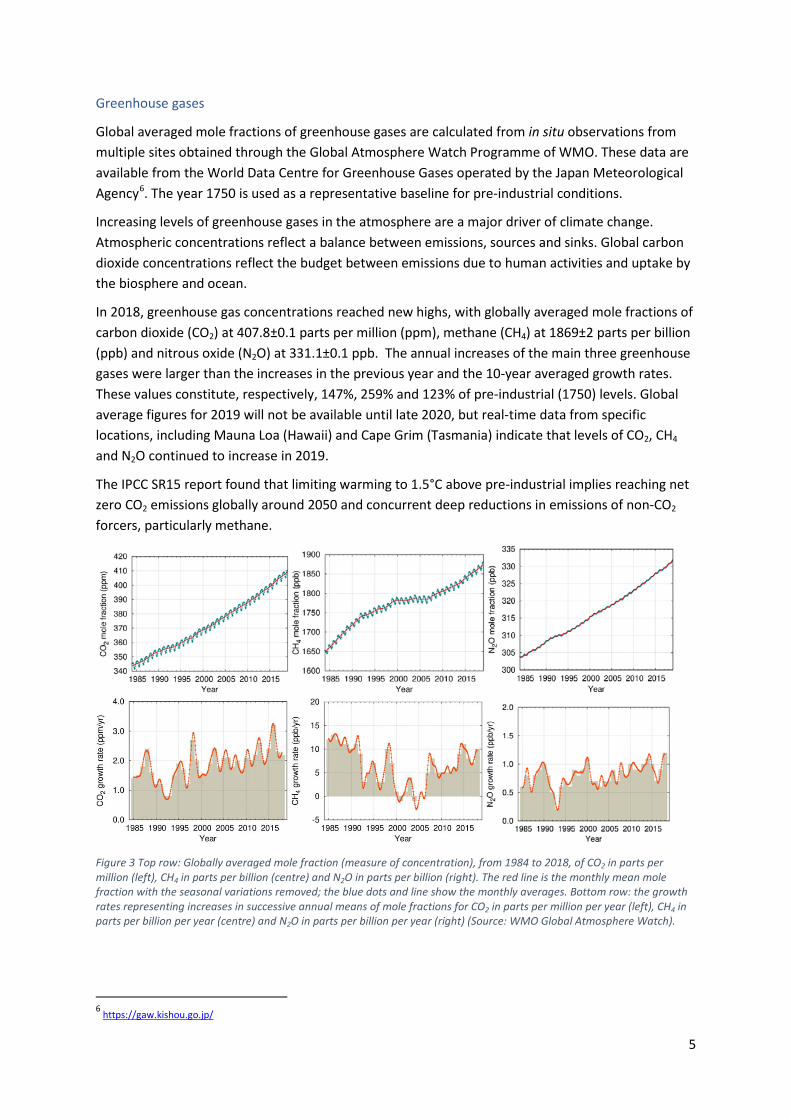
Global averaged mole fractions of greenhouse gases are calculated from in situ observations from multiple sites obtained through the Global Atmosphere Watch Programme of WMO. These data are available from the World Data Centre for Greenhouse Gases operated by the Japan Meteorological Agency6. The year 1750 is used as a representative baseline for pre-industrial conditions.

Increasing levels of greenhouse gases in the atmosphere are a major driver of climate change. Atmospheric concentrations reflect a balance between emissions, sources and sinks. Global carbon dioxide concentrations reflect the budget between emissions due to human activities and uptake by the biosphere and ocean.

In 2018, greenhouse gas concentrations reached new highs, with globally averaged mole fractions of carbon dioxide (CO2) at 407.8±0.1 parts per million (ppm), methane (CH4) at 1869±2 parts per billion (ppb) and nitrous oxide (N2O) at 331.1±0.1 ppb. The annual increases of the main three greenhouse gases were larger than the increases in the previous year and the 10-year averaged growth rates. These values constitute, respectively, 147%, 259% and 123% of pre-industrial (1750) levels. Global average figures for 2019 will not be available until late 2020, but real-time data from specific locations, including Mauna Loa (Hawaii) and Cape Grim (Tasmania) indicate that levels of CO2, CH4 and N2O continued to increase in 2019.

The IPCC SR15 report found that limiting warming to 1.5°C above pre-industrial implies reaching net zero CO2 emissions globally around 2050 and concurrent deep reductions in emissions of non-CO2 forcers, particularly methane.

Figure 3 Top row: Globally averaged mole fraction (measure of concentration), from 1984 to 2018, of CO2 in parts per million (left), CH4 in parts per billion (centre) and N2O in parts per billion (right). The red line is the monthly mean mole fraction with the seasonal variations removed; the blue dots and line show the monthly averages. Bottom row: the growth rates representing increases in successive annual means of mole fractions for CO2 in parts per million per year (left), CH4 in parts per billion per year (centre) and N2O in parts per billion per year (right) (Source: WMO Global Atmosphere Watch).

6 https://gaw.kishou.go.jp/

6

Oceans

The ocean is an important part of the Earth system. The rate of change in ocean heat content is a measure of global warming, as it represents the heat accumulating in the climate system. Thermal expansion from the ocean warming leads to sea level rise, which has impacts along the coasts. Changes in ocean chemistry associated with rising CO2 concentrations in the atmosphere are altering the pH of the oceans.

Ocean heat content

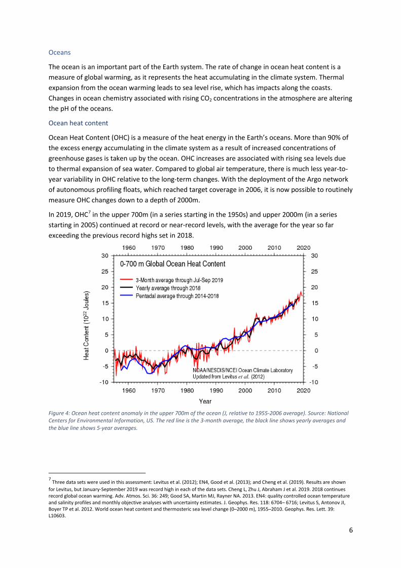
Ocean Heat Content (OHC) is a measure of the heat energy in the Earth’s oceans. More than 90% of the excess energy accumulating in the climate system as a result of increased concentrations of greenhouse gases is taken up by the ocean. OHC increases are associated with rising sea levels due to thermal expansion of sea water. Compared to global air temperature, there is much less year-to-year variability in OHC relative to the long-term changes. With the deployment of the Argo network of autonomous profiling floats, which reached target coverage in 2006, it is now possible to routinely measure OHC changes down to a depth of 2000m.

In 2019, OHC7 in the upper 700m (in a series starting in the 1950s) and upper 2000m (in a series starting in 2005) continued at record or near-record levels, with the average for the year so far exceeding the previous record highs set in 2018.

Figure 4: Ocean heat content anomaly in the upper 700m of the ocean (J, relative to 1955-2006 average). Source: National Centers for Environmental Information, US. The red line is the 3-month average, the black line shows yearly averages and the blue line shows 5-year averages.

7 Three data sets were used in this assessment: Levitus et al. (2012); EN4, Good et al. (2013); and Cheng et al. (2019). Results are shown for Levitus, but January-September 2019 was record high in each of the data sets. Cheng L, Zhu J, Abraham J et al. 2019. 2018 continues record global ocean warming. Adv. Atmos. Sci. 36: 249; Good SA, Martin MJ, Rayner NA. 2013. EN4: quality controlled ocean temperature and salinity profiles and monthly objective analyses with uncertainty estimates. J. Geophys. Res. 118: 6704– 6716; Levitus S, Antonov JI, Boyer TP et al. 2012. World ocean heat content and thermosteric sea level change (0–2000 m), 1955–2010. Geophys. Res. Lett. 39: L10603.

7

Marine heatwaves As over land, extreme heat can affect the near-surface oceans with a range of impacts for marine life and dependent communities. Satellite retrievals of sea-surface temperature can be used to monitor marine heatwaves (MHW). In this case a moderate MHW is defined as a period when the sea-surface temperature is above the 90th percentile of the climatological distribution for five days or longer8. A strong heatwave is declared if the difference from the long-term average is more than twice as large as the difference at the 90th percentile. A severe heatwave if it is more than three times as large and an extreme heatwave at more than four times.

For 2019 to date (18 November 2019, Figure 5) the number of MHW days averaged over the entire ocean was approximately 45 days per pixel. This means that so far in 2019, the ocean has on average experienced around 1.5 months of unusually warm temperatures. More of the ocean had a MHW classified as "Strong" (38%) than "Moderate" MHWs (28%). In the north-east Pacific, large areas reached a MHW category of “Severe”. From 2014 to 2016, sea-surface temperature in the area were also unusually high and the mass of warmer-than-average waters was dubbed the “blob”9,10. Another notable area is the Tasman Sea, where there has been a series of MHWs in the summers of 2015-1611, 2017-1812 and again in 2018-19. Climate events including MHWs and floods were associated with extensive mortality of key marine habitat-forming communities along more than 45% of Australia’s continental coastline between 2011 and 201713.

8 Hobday, A.J., E.C.J. Oliver, A. Sen Gupta, J.A. Benthuysen, M.T. Burrows, M.G. Donat, N.J. Holbrook, P.J. Moore, M.S. Thomsen, T. Wernberg, and D.A. Smale. 2018. Categorizing and naming marine heatwaves. Oceanography 31(2), https://doi.org/10.5670/oceanog.2018.205. 9 Gentemann, C. L., Fewings, M. R., and García-Reyes, M. (2017), Satellite sea surface temperatures along the West Coast of the United States during the 2014–2016 northeast Pacific marine heat wave, Geophys. Res. Lett., 44, 312– 319, doi:10.1002/2016GL071039. 10 Di Lorenzo, E. and Mantua, N., 2016. Multi-year persistence of the 2014/15 North Pacific marine heatwave. Nature Climate Change, 6(11), p.1042. 11 Oliver, E.C., Benthuysen, J.A., Bindoff, N.L., Hobday, A.J., Holbrook, N.J., Mundy, C.N. and Perkins-Kirkpatrick, S.E., 2017. The unprecedented 2015/16 Tasman Sea marine heatwave. Nature communications, 8, p.16101. 12 Perkins-Kirkpatrick, S.E., King, A.D., Cougnon, E.A., Holbrook, N.J., Grose, M.R., Oliver, E.C.J., Lewis, S.C. and Pourasghar, F., 2019. The role of natural variability and anthropogenic climate change in the 2017/18 Tasman Sea marine heatwave. Bulletin of the American Meteorological Society, 100(1), pp.S105-S110. 13 Babcock, R. C., R. H. Bustamante, E. A. Fulton, D. J. Fulton, M. D. E. Haywood, A. J. Hobday, R. Kenyon, R. J. Matear, E. E. Plagányi, A. J. Richardson, and M. A. Vanderklift. 2019. Severe Continental-Scale Impacts of Climate Change Are Happening Now: Extreme Climate Events Impact Marine Habitat Forming Communities Along 45% of Australia’s Coast. Frontiers in Marine Science 6.

8

Figure 5: (a) Global map showing the highest category experienced at each pixel over the course of the year estimated using the NOAA OI v2 data set. Light grey shows that no MHWs occurred in a pixel over the entire year. (b) Stacked barplot showing the percent of ocean pixels experiencing a MHW on any given day of the year, (c) Stacked barplot showing the cumulative percent of the ocean that has experienced a MHW over the year. These values are based on when in the year a pixel first experiences it's highest category MHW, so no pixel is counted more than once. Horizontal bars in this figure show the final percentage values for each category of MHW. (d) Stacked barplot showing the cumulative number of MHW days averaged over all pixels in the ocean. This is taken by finding the cumulative MHW days per pixel for the entire ocean and dividing that by the overall number of ocean pixels (~690,000). Source: Robert Schlegel, Woods Hole.

Sea level

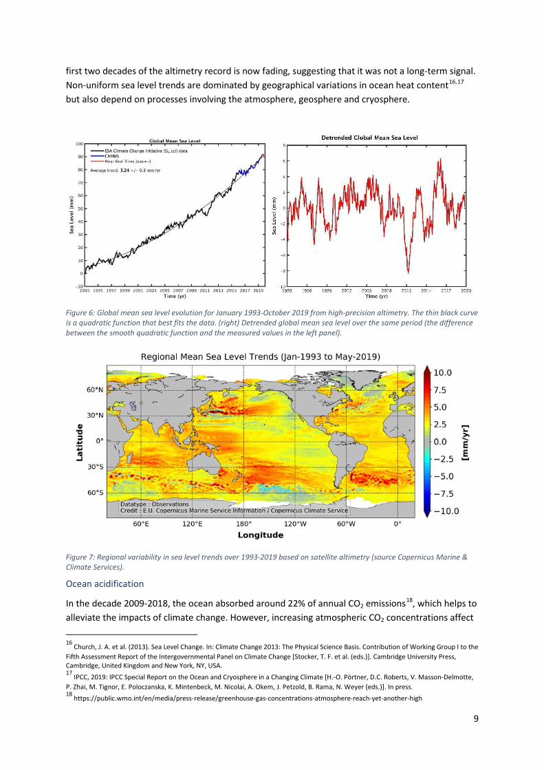
In 2019, sea level has continued to rise (Figure 6, left; last update 17 October 2019). In October 2019, the global mean sea level reached its highest value since the beginning of the high-precision altimetry record (January 1993). The average rate of rise is estimated to be 3.25 ± 0.3 mm/yr over the 27-year long period, but the rate has increased over that time. Increased ice mass loss from the ice sheets is the main cause of the global mean sea-level acceleration14.

Interannual variability (Figure 6, right) in sea-level rise is mainly driven by the El Niño Southern Oscillation (ENSO, see also the section on Drivers). During El Niño, water from tropical river basins on land is transferred to the ocean (e.g., in 1997, 2012 and 2015). During La Niña, the opposite occurs, with a transfer of water from the ocean to land (e.g., in 2011)15.

Sea level rise is not regionally uniform. Figure 7 shows the spatial trend patterns from January 1993 to May 2019. The strongest regional trends in the southern hemisphere are east of Madagascar in the Indian Ocean, east of New-Zealand in the Pacific Ocean, and east of Rio de la Plata/South America in the south Atlantic. In the northern hemisphere, an eastward, elongated pattern is also seen in the north Pacific. A previously-strong pattern seen in the western tropical Pacific over the

14 World Climate Research Programme Global Sea Level Budget Group, 2018: Global sea-level budget 1993–present. Earth Systems Science Data, 10:1551–1590. 15 Fasullo, J. T., Boening, C., Landerer, F.W., Nerem, R.S. (2013). Australia's unique influence on global sea level in 2010–2011, Geophysical Research Letters, 40, 4368–4373, doi:10.1002/grl.50834.

9

first two decades of the altimetry record is now fading, suggesting that it was not a long-term signal. Non-uniform sea level trends are dominated by geographical variations in ocean heat content16,17 but also depend on processes involving the atmosphere, geosphere and cryosphere.

Figure 6: Global mean sea level evolution for January 1993-October 2019 from high-precision altimetry. The thin black curve is a quadratic function that best fits the data. (right) Detrended global mean sea level over the same period (the difference between the smooth quadratic function and the measured values in the left panel).

Figure 7: Regional variability in sea level trends over 1993-2019 based on satellite altimetry (source Copernicus Marine & Climate Services).

Ocean acidification

In the decade 2009-2018, the ocean absorbed around 22% of annual CO2 emissions18, which helps to alleviate the impacts of climate change. However, increasing atmospheric CO2 concentrations affect

16 Church, J. A. et al. (2013). Sea Level Change. In: Climate Change 2013: The Physical Science Basis. Contribution of Working Group I to the Fifth Assessment Report of the Intergovernmental Panel on Climate Change [Stocker, T. F. et al. (eds.)]. Cambridge University Press, Cambridge, United Kingdom and New York, NY, USA. 17 IPCC, 2019: IPCC Special Report on the Ocean and Cryosphere in a Changing Climate [H.-O. Pörtner, D.C. Roberts, V. Masson-Delmotte, P. Zhai, M. Tignor, E. Poloczanska, K. Mintenbeck, M. Nicolai, A. Okem, J. Petzold, B. Rama, N. Weyer (eds.)]. In press. 18 https://public.wmo.int/en/media/press-release/greenhouse-gas-concentrations-atmosphere-reach-yet-another-high

10

the chemistry of the ocean. CO2 reacts with seawater and alters the acidity of the ocean by decreasing its pH. This process is called ocean acidification. The change of pH is linked to other shifts in carbonate chemistry that decrease the ability of a variety of marine organisms to calcify, from mussels and crustaceans to corals. The changes in CO2 concentration, pH and carbonate chemistry affect marine life, lessening the potential for growth and reproduction.

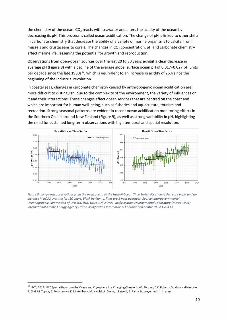
Observations from open-ocean sources over the last 20 to 30 years exhibit a clear decrease in average pH (Figure 8) with a decline of the average global surface ocean pH of 0.017–0.027 pH units per decade since the late 1980s19, which is equivalent to an increase in acidity of 26% since the beginning of the industrial revolution.

In coastal seas, changes in carbonate chemistry caused by anthropogenic ocean acidification are more difficult to distinguish, due to the complexity of the environment, the variety of influences on it and their interactions. These changes affect ocean services that are centred on the coast and which are important for human well-being, such as fisheries and aquaculture, tourism and recreation. Strong seasonal patterns are evident in recent ocean acidification monitoring efforts in the Southern Ocean around New Zealand (Figure 9), as well as strong variability in pH, highlighting the need for sustained long-term observations with high temporal and spatial resolution.

Figure 8: Long-term observations from the open ocean at the Hawaii Ocean Time Series site show a decrease in pH and an increase in pCO2 over the last 30 years. Black horizontal lines are 5-year averages. Source: Intergovernmental Oceanographic Commission of UNESCO (IOC-UNESCO), NOAA Pacific Marine Environmental Laboratory (NOAA PMEL), International Atomic Energy Agency Ocean Acidification International Coordination Centre (IAEA OA-ICC).

19 IPCC, 2019: IPCC Special Report on the Ocean and Cryosphere in a Changing Climate [H.-O. Pörtner, D.C. Roberts, V. Masson-Delmotte, P. Zhai, M. Tignor, E. Poloczanska, K. Mintenbeck, M. Nicolai, A. Okem, J. Petzold, B. Rama, N. Weyer (eds.)]. In press.

11

Figure 9: Measurements of pH from four sites around New Zealand, spanning between four and five years of observations: Urbanised sites in Auckland and Wellington (top row), one open coast (Jackson Bay) and one Bay (Tasman Bay) site in the bottom row. Seasonal patterns and great variability between pH measurements are clearly visible. Credit: Kim Currie (NIWA).

Deoxygenation Both observations and numerical models indicate that oxygen is declining in the modern open and coastal oceans, including estuaries and semi-enclosed seas. Since the middle of the last century, there has been an estimated 1%–2% decrease (that is, 2.4–4.8 Pmol or 77 billion–145 billion tons) in the global ocean oxygen inventory20,21.

The projected expansion of the pre-industrial area of oxygen minima (< 80 µmol kg-1) by 7% through 2100 is expected to alter the diversity, composition, abundance, and distribution of marine life22. New studies further identified deoxygenation alongside ocean warming and ocean acidification as a major threat to ocean ecosystems and human well-being23. Even coral reefs are now recognized as vulnerable to major oxygen loss24.

20 Bopp, L., L. Resplandy, J.C. Orr, S.C. Doney, J.P. Dunne, M. Gehlen, P. Halloran, C. Heinze, T. Ilyina and R. Seferian, 2013: Multiple stressors of ocean ecosystems in the 21st century: projections with CMIP5 models. Biogeosciences, 10:6225–6245.

21 Schmidtko, S., L. Stramma and M. Visbeck, 2017: Decline in global oceanic oxygen content during the past five decades. Nature, 542:335–339 22 IPCC. (2019). Summary for Policymakers. In: IPCC Special Report on the Ocean and Cryosphere in a Changing Climate [H.-O. Pörtner, D.C. Roberts, V. Masson-Delmotte, P. Zhai, M. Tignor, E. Poloczanska, K. Mintenbeck, M. Nicolai, A. Okem, J. Petzold, B. Rama, N. Weyer (eds.)]. In press. 23 IPCC. (2019). Summary for Policymakers. In: IPCC Special Report on the Ocean and Cryosphere in a Changing Climate [H.-O. Pörtner, D.C. Roberts, V. Masson-Delmotte, P. Zhai, M. Tignor, E. Poloczanska, K. Mintenbeck, M. Nicolai, A. Okem, J. Petzold, B. Rama, N. Weyer (eds.)]. In press. 24 Camp EF, Nitschke MR, Rodolfo-Metalpa R, Houlbreque F, Gardner SG, Smith DJ, Zampighi M and Suggett DJ. (2017). Reef-building corals thrive within hot-acidified and deoxygenated waters. Scientific reports, 7(1), 2434.

12

Cryosphere

The cryosphere component of the Earth system includes solid precipitation, snow cover, sea ice, lake and river ice, glaciers, ice caps, ice sheets, permafrost and seasonally frozen ground. The cryosphere provides key indicators of a changing climate, yet it is one of the most under-sampled domains of the Earth system. Many of the components are measured at the surface, but spatial coverage is generally poor. Some, like sea ice extent, have been measured from space for many years, while the capability to measure other components from space is still developing. The major cryosphere indicators for the provisional statement include sea-ice extent and the Greenland ice sheet mass balance.

Sea ice

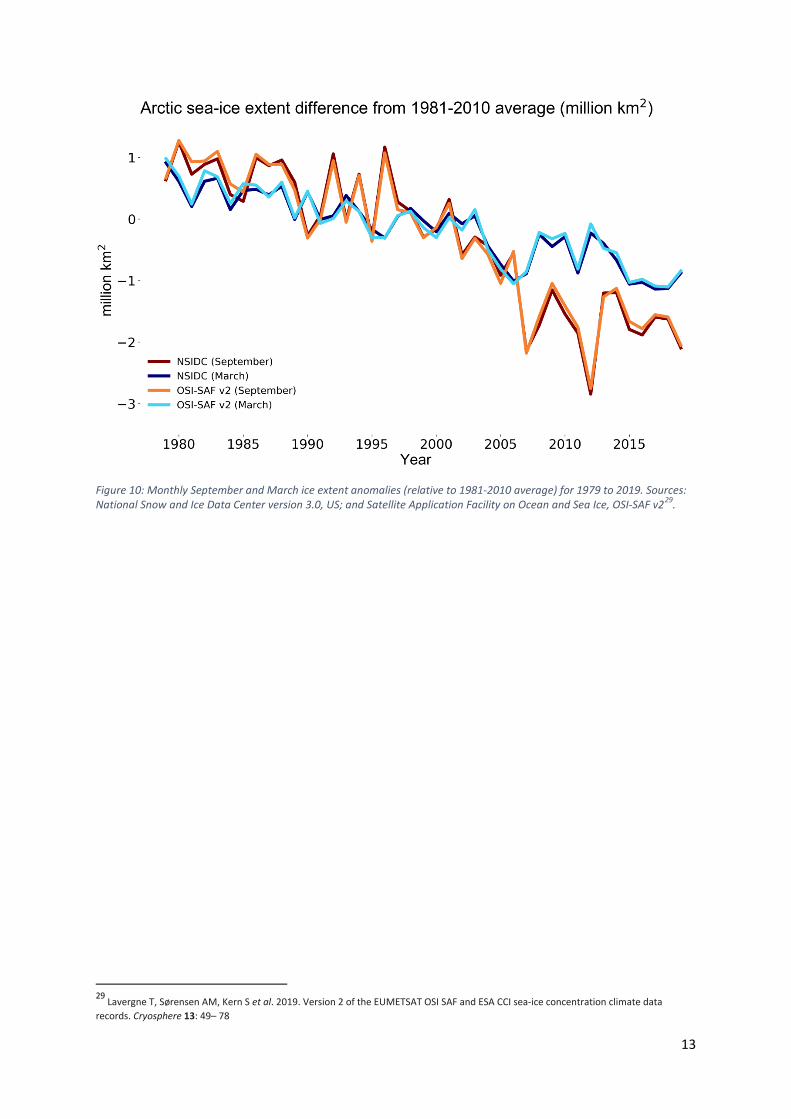
Arctic (as well as sub-Arctic) sea ice has seen a long-term decline in all months during the satellite era (1979-present, Figure 10), with the largest relative losses in late summer around the time of the annual minimum, with regional variations.

The 2019 Arctic winter maximum daily sea-ice extent (14.78 million square kilometres), reached around 13 March, was the 7th lowest maximum on record25 and the March monthly average was also the 7th lowest (Figure 10). From April to October 2019, daily extents remained low and monthly extents were among the three lowest on record for those months.

The Arctic summer minimum daily sea-ice extent (4.15 million square kilometres), which occurred around 18 September, was tied with 2007 and 2016 for the 2nd lowest on record26 (Figure 11, bottom). The September monthly-average extent was the nominally the 3rd lowest on record27 (Figure 10). Extents remained very low till November, with the ice edge advancing more slowly than normal in the Beaufort, Chukchi, Kara and Barents Seas. Around Svalbard, however, the sea ice returned to near average conditions28. The monthly extent for October was the lowest on record.

25 http://nsidc.org/arcticseaicenews/2019/03/ 26 http://nsidc.org/arcticseaicenews/2019/09/ 27 http://nsidc.org/arcticseaicenews/2019/10/ 28 http://nsidc.org/arcticseaicenews/2019/11/

13

Figure 10: Monthly September and March ice extent anomalies (relative to 1981-2010 average) for 1979 to 2019. Sources: National Snow and Ice Data Center version 3.0, US; and Satellite Application Facility on Ocean and Sea Ice, OSI-SAF v229.

29 Lavergne T, Sørensen AM, Kern S et al. 2019. Version 2 of the EUMETSAT OSI SAF and ESA CCI sea-ice concentration climate data records. Cryosphere 13: 49– 78

14

Figure 11: Blended Arctic ice chart (AARI, CIS, NIC) for 16-19 September 2019 and ice edge occurrences for 16-20 September for 1979-2018 with colouring based on ice total concentration. Source: AARI.

Ice conditions varied strongly during the 2018/19 winter in the Arctic regional seas. Although ice extent was extremely low in the Bering Sea, it was close to normal in the adjacent Sea of Okhotsk. Northerly winds in the Barents Sea region from January to August 2019 meant that ice extent was close to normal in the northern part of this area, unlike the past decade when it was lower than average. Winter 2018/19 brought early ice formation on the North American Great Lakes and above-average ice coverage. The maximum ice coverage on the Great Lakes was 145% of the long-term average and was the 7th highest since 1972/7330.

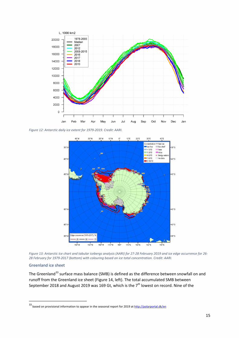
Until 2016, Antarctic sea ice extent had shown a small long-term increase. In late 2016 this was interrupted by a sudden drop in extent to extreme low values. Since then, Antarctic sea-ice extent has remained at relatively low levels. 2019 saw a number of months with record low monthly extents (May, June and July), but late Austral winter and spring saw extents that were closer to the long-term average (Figure 12). The minimum daily sea-ice extent (2.47 million square kilometres), reached around 28 February31 (Figure 13), was the 7th lowest on record. The maximum daily sea-ice extent (18.40 million square kilometres), was reached around 30 September32 (Figure 13).

30 https://www.glerl.noaa.gov/data/ice/#historical 31 http://nsidc.org/arcticseaicenews/2019/03/ 32 http://nsidc.org/arcticseaicenews/2019/10/

15

Figure 12: Antarctic daily ice extent for 1979-2019. Credit: AARI.

Figure 13: Antarctic Ice chart and tabular icebergs analysis (AARI) for 27-28 February 2019 and ice edge occurrence for 26-28 February for 1979-2017 (bottom) with colouring based on ice total concentration. Credit: AARI.

Greenland ice sheet

The Greenland33 surface mass balance (SMB) is defined as the difference between snowfall on and runoff from the Greenland ice sheet (Figure 14, left). The total accumulated SMB between September 2018 and August 2019 was 169 Gt, which is the 7th lowest on record. Nine of the

33 based on provisional information to appear in the seasonal report for 2019 at http://polarportal.dk/en

16

10 lowest SMB years since 1981 have been observed in the last 13 years. For comparison, the average SMB for 1981-2010 is 368 Gt, and the lowest SMB was 38 Gt in 2012.

SMB is always positive at the end of the year, but the ice sheet also loses ice through calving of icebergs and melting via the contact of glacier tongues with warm sea water. With satellites we can measure the ice velocity of the outlet glaciers around the edges of the ice sheet and from that we can estimate how much ice is lost by calving and ocean melting. The analysis for 2018/19 gives a loss of about 498 Gt. For comparison, the ice sheet lost an average of about 462 Gt per year as icebergs and via ocean melting over the period 1986-2018.

Combining a gain in SMB of 169 Gt with ice loss from calving and ocean melting of 498 Gt gives a net ice loss for 2018/19 of 329 Gt. To put this into context, data from the Gravity Recovery and Climate Experiment (GRACE) satellites tell us that Greenland lost about 260 Gt of ice per year over the period 2002-2016, with a maximum of 458 Gt in 2011/12. So, the 329 Gt of this season is well above the average but is not a record loss.

Figure 14: (left) Surface Mass Balance for the “SMB year” 1 September 2018 to 31 August 2019. The upper panel shows individual days, and the lower panel shows the accumulated sum over the year. 2018/19 is in blue, and the grey line is the long-term average. For comparison, the lower panel also shows the record year 2011/12 in red. Units are gigatonnes (Gt) per day and gigatonnes, respectively. (right) map shows SMB anomaly (in mm) across Greenland. SMB was below normal almost everywhere in Greenland except the southeast. This was due to a dry winter, a very early start of the melting season and a long dry and warm summer. Source: Polar Portal, http://polarportal.dk/en.

Drivers of short-term climate variability

The ocean plays a number of important roles in the climate. Surface temperatures change relatively slowly over the ocean so recurring patterns in sea-surface temperature can be used to understand and, in some cases, predict the more rapidly-changing patterns of weather over land on seasonal time scales. Two factors in particular that can help to understand the climate of 2019 are the El Niño Southern Oscillation and the Indian Ocean Dipole.

17

El Niño Southern Oscillation (ENSO)

The El Niño Southern Oscillation is one of the most important drivers of year-to-year variability in global weather patterns. El Niño events, characterised by warmer than average sea-surface temperatures in the eastern Pacific and a weakening of the trade winds, are associated with higher global temperatures. Cooler global temperatures often accompany La Niña events, which are characterised by cooler than average sea-surface temperatures in the eastern Pacific and a strengthening of the trade winds. For example, record global temperatures in 2016 followed an unusually strong El Niño event.

In contrast, 2019 started with neutral or weak El Niño conditions34. Sea-surface temperatures reached or exceeded typical El Niño thresholds from October 2018 through the first half of 2019, but an atmospheric response was absent in the early stages of the event. Atmospheric indicators such as weakened trade winds and increased cloudiness at the dateline did not show consistently until February. Thereafter, coupling between the ocean and atmosphere maintained sea-surface temperatures at borderline El Niño levels to the middle of the year.

Indian Ocean Dipole (IOD)

The positive phase of the IOD is characterised by cooler than average sea-surface temperatures in the eastern Indian Ocean and warmer than average sea-surface temperatures in the west. The negative phase has the opposite pattern. The resulting change in the gradient of sea-surface temperature across the ocean basin affects the weather of the surrounding continents.

In 2019, the IOD started weakly positive and became progressively more positive from May to October, ultimately becoming one of the strongest positive IOD events since reliable records began around 1960. The positive phase of the IOD during austral winter and spring has been associated with drier and warmer conditions over Indonesia and surrounding countries, and parts of Australia. Indeed, Australia has seen unusually dry conditions during winter and spring exacerbating long-term rainfall deficits. Indonesia and Singapore also experienced dry conditions. The positive IOD is also linked to late Indian southwest monsoon withdrawal as was observed this year, and high rainfall in the later part of the year in east Africa. For more details on regional impacts, see the sections on “Heavy rainfall and floods” and “Drought”.

High-impact events in 2019 The following sections describe a selection of high-impact events in 2019. Information on such events is largely based on contributions from WMO Members with additional information from the Global Precipitation Climatology Centre (GPCC), Regional Climate Centres, and tropical storm monitoring centres.

Heat and cold waves 2019 was another year which saw numerous major heatwaves. Amongst the most significant were two major heatwaves which occurred in Europe in late June and late July. The first heatwave reached its maximum intensity in southern France, where a national record of 46.0°C (1.9°C above the previous record) was set on 28 June at Vérargues (Hérault). It also affected much of western Europe. The second heatwave was more extensive, with national records set in Germany (42.6°C),

34 http://www.wmo.int/pages/prog/wcp/wcasp/documents/WMO_ENSO_May19_Eng.pdf

18

the Netherlands (40.7°C), Belgium (41.8°C), Luxembourg (40.8°C) and the United Kingdom (38.7°C), with the heat also extending into the Nordic countries, where Helsinki had its highest temperature on record (33.2°C on 28 July). At some long-term stations, records were broken by 2°C or more, including Paris, where 42.6°C at the main Montsouris observatory on 25 July was 2.2°C above the previous record set in 1947, and Uccle (near Brussels), whose 39.7°C was 3.1°C above the previous record. In France, a total of around 1 462 (uncertainty range 548 to 2 221) excess deaths were reported35 (for more detail see Section on Extreme Heat and Health).

Japan experienced two heatwaves that were notable in different ways. The first occurred in late May, with unusually high temperatures, including 39.5°C (the equal-highest on record for any time of year on the island of Hokkaido), but limited impacts. The second, in July, was less unusual in a meteorological sense but had much greater health impacts as it occurred during the peak of summer and was focused in the more heavily populated area of Honshu.

Australia had an exceptionally hot summer. The mean summer temperature was the highest on record by almost 1°C, and January was Australia’s hottest month on record. Most of the country was affected, with the most extreme anomalies occurring in inland New South Wales. The heat was most notable for its persistence but there were also significant individual extremes, including 46.6°C at Adelaide on 24 January, the city’s highest temperature on record. The heat extended to New Zealand at the end of January, with record highs on 29 January at Hamilton (32.9°C) and Wellington (30.3°C), and significant wildfires in the north of the South Island.

Another major heatwave of the Southern Hemisphere summer occurred in southern South America in late January and early February. The initial stage of the heatwave peaked in central Chile, with records set in a number of locations, including Santiago (38.3°C on 27 January). The following week, exceptionally high temperatures reached the far south of the continent. 30.8°C at Rio Grande (Argentina, 53.8°S) on 4 February is believed to be the southernmost recorded instance of a temperature of 30°C.

Whilst the absolute highest temperatures in the Middle East were not as high as some of those observed in recent years, there were still some noteworthy observations. 49.9°C at Sedom on 17 July was Israel’s highest temperature since at least 1942. Extreme heat also affected the Indian subcontinent in the pre-monsoon period in May and early June. A number of record high temperatures were set in India, including 48.0°C at New Delhi Airport on 10 June.

Consistent with a warm year globally and an overall warming trend, extreme cold was less common than extreme heat. One area of below-average temperature for January to October 2019 was North America (Figure 2). The year’s most significant cold spell was in late winter in central North America. This started with an intense cold wave in the United States Midwest in late January, including an Illinois state record of −38.9°C at Mount Carroll on 31 January, followed by very persistent cold through February and early March in the interior west on both sides of the United States-Canada border. February mean temperatures were more than 15°C below normal in places, including Great Falls (Montana), whose monthly mean of −17.9°C was 15.3°C below normal and more than 5°C below the previous record, whilst it was also the coldest February on record for several regions in western Canada, including the city of Vancouver. It was also a rather cold first half of the year in parts of eastern Canada. There were further outbreaks of unseasonable cold and early-season 35 https://www.santepubliquefrance.fr/determinants-de-sante/climat/fortes-chaleurs-canicule/documents/bulletin-national/bulletin-de-sante-publique-canicule.-bilan-ete-2019

19

snowfall in the western and central interior of North America in late September and late October. Record low temperatures for October were set for eight states in the northern and western United States in late October, in marked contrast to the record high temperatures for the month set in ten southern and eastern states early in the month. The first half of November was also abnormally cold in many parts of the northern United States and southern Canada.

While temperatures were near or above average, very heavy winter and early spring precipitation led to an unusually heavy snowpack in many parts of the European Alps. More than 300 cm of snow fell in parts of the Austrian Alps between 4 and 15 January, whilst spring snowfalls led to a record high snow depth for 1 June of 270 cm at Weissfluhjoch (Switzerland, 2540 m elevation), although very hot weather in June led to that snow melting by early July, close to the normal start of the snow-free period. Numerous avalanches were reported throughout the region during the heaviest snowfall periods.

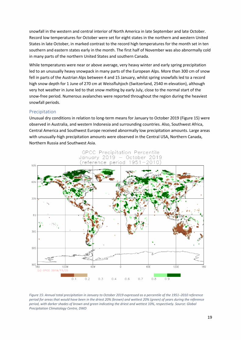
Precipitation Unusual dry conditions in relation to long-term means for January to October 2019 (Figure 15) were observed in Australia, and western Indonesia and surrounding countries. Also, Southwest Africa, Central America and Southwest Europe received abnormally low precipitation amounts. Large areas with unusually-high precipitation amounts were observed in the Central USA, Northern Canada, Northern Russia and Southwest Asia.

Figure 15: Annual total precipitation in January to October 2019 expressed as a percentile of the 1951–2010 reference period for areas that would have been in the driest 20% (brown) and wettest 20% (green) of years during the reference period, with darker shades of brown and green indicating the driest and wettest 10%, respectively. Source: Global Precipitation Climatology Centre, DWD

20

There was a large precipitation deficit in India in June as the onset of the Monsoon was delayed. However, associated with the positive Indian Ocean Dipole, the withdrawal of the Indian Monsoon was also delayed and there was an excess of precipitation in the following months for most regions.

Heavy rainfall and floods Regular flooding occurred during the Indian summer monsoon season, particularly in western and northern India and neighbouring countries. Overall all-India rainfall for the summer monsoon season (June-September) was 10% above the 1961-2010 average, the first above-average year since 2013 and the wettest since 1994, despite a below-average June. The retreat of the monsoon was also exceptionally late, with the withdrawal date of 9 October the latest on record. Over 1 000 lives were reported to have been lost in various flooding episodes in India during the season. Monsoonal flooding also affected parts of southern China in June, with 83 deaths and over US$2.5 billion in economic losses reported.

The Islamic Republic of Iran was badly affected by flooding in late March and early April, with the Shiraz region being the worst-affected. 24-hour rainfall totals during the event were as high as 188 mm. The impact of the event was severe, with at least 76 deaths reported and severe economic losses.

A tropical low brought extreme rainfall and associated flooding in northern Queensland (Australia) in late January and early February. Rainfall totals over a 10-day period exceeded 2000 mm in some coastal areas around Townsville, with Townsville itself receiving 1259.8 mm36, whilst a second episode of heavy rain in inland northwest Queensland brought 7-day totals exceeding 600 mm. There was major urban flooding in the Townsville area, whilst in northwest Queensland some rivers expanded to tens of kilometres wide. The flooding and associated unusually cool weather led to heavy livestock losses. Total economic losses were estimated to be in the order of US$2 billion37.

In March, flash flooding and associated landslides occurred around Jayapura in the Indonesian province of Papua after rainfall of 235 mm in 8 hours, with at least 112 deaths reported. Later, an influx of tropical moisture brought extreme rainfall to the west coast of New Zealand’s South Island in late March, with a national 48-hour record of 1086 mm at Cropp River, with associated major flooding. A bridge on the region’s main highway was washed away.

Persistent heavy rainfall affected a large part of the central United States in late 2018 and the first half of 2019. The 12-month rainfall averaged over the contiguous United States for the period for July 2018 to June 2019 (962 mm) was the highest on record. This led to long-lived flooding in the Mississippi basin, with the river remaining above flood stage at Baton Rouge (Louisiana) for nearly seven months from 6 January to 4 August. There was also significant flooding in parts of eastern Canada in April and early May due to a combination of heavy rain and rapid melting of an above-average snowpack, particularly in the Ottawa and Montreal areas and in New Brunswick.

Very wet conditions affected parts of South America in January. There was major flooding in northern Argentina, Uruguay and southern Brazil, with losses in Argentina and Uruguay estimated at US$2.5 billion. January monthly totals exceeded 600 mm at a number of sites in northeast Argentina.

36 http://www.bom.gov.au/climate/current/statements/scs69.pdf 37 http://thoughtleadership.aonbenfield.com/Documents/20191107_analytics-if-october-global-recap.pdf

21

Major flooding affected many hitherto drought-affected parts of east Africa in October and early November, after heavy rains associated with the positive Indian Ocean Dipole occurred. October monthly totals exceeded 400 mm in parts of the region. Somalia, Kenya, Tanzania, Ethiopia and South Sudan were all significantly affected. Earlier in the year, flooding during the rainy season affected a number of countries, including Sudan, Nigeria, Cameroon and Côte d’Ivoire, although overall Sahel seasonal rainfall was mostly fairly close to average.

Tropical cyclones Tropical cyclone activity globally in 2019 (to 17 November) was slightly above average. The Northern Hemisphere, to date, has had 66 tropical cyclones, compared with the average at this time of year of 56, although accumulated cyclone energy (ACE) was only 2% above average. The 2018-19 Southern Hemisphere season was also above average, with 27 cyclones, the most in a season since 2008-09.

It was a particularly extreme cyclone season in the North Indian Ocean. Three cyclones reached maximum sustained winds of 100 knots or more, the first known instance in a single season, and the ACE for the season was the highest on record by a large margin. Cyclone Fani was the most significant cyclone to affect India since 2013, making landfall in the east of the country on the Odisha coast on 3 May with sustained winds of 100 knots, having earlier peaked at 135 knots in the Bay of Bengal. There was significant damage in coastal areas and loss of life, although extensive evacuations in affected coastal areas greatly reduced the impact. Cyclone Kyarr in October was one of the strongest cyclones on record in the Arabian Sea, but did not make landfall, although associated high seas and storm surges had some coastal impacts.

The south Indian Ocean basin also had an active season; there were 18 cyclones of which 13 reached hurricane intensity, the equal largest number on record. Tropical Cyclone Idai made landfall near Beira (Mozambique) on 15 March, having had maximum sustained winds of 105 knots. It was one of the strongest known cyclones to make landfall on the east coast of Africa. There was widespread destruction from wind and storm surge in coastal Mozambique, especially in the city of Beira, whilst severe flooding extended to inland regions of Mozambique and parts of Zimbabwe, particularly the northeast. Later the same month, another severe cyclone, Kenneth, made landfall in northern Mozambique, although it hit a more sparsely populated region and impacts were less severe.

One of the year’s most intense tropical cyclones was Dorian, which reached category 5 intensity in the western Atlantic at the end of August, making landfall in the Bahamas on 1 September with maximum sustained winds of 165 knots, the equal-highest on record for a North Atlantic landfall. Dorian was also exceptionally slow-moving and remained near-stationary over the Bahamas as a category 5 system for about 24 hours. The prolonged extreme winds and storm surge led to near-total destruction on a number of islands of the Bahamas, with at least 60 deaths reported38 and economic losses in the Bahamas estimated at more than US$3 billion39. Dorian then moved northeast, with significant damage recorded on parts of the United States east coast and in the Canadian province of Nova Scotia. Tropical Storm Imelda brought extreme rainfall to some of the areas of far eastern Texas also hit by Hurricane Harvey in 2017, with rainfall totals of over 1000 mm in places. Two other storms noteworthy for their eastern location were Lorenzo, the easternmost

38 https://reliefweb.int/report/bahamas/hurricane-dorian-situation-report-14-october-15-2019#:~:targetText=SITUATION%20UPDATE,strongest%20hurricane%20in%20modern%20records. Has 61 deaths confirmed in October according to the Royal Bahamas Police Force 39 https://www.iadb.org/en/damages-and-other-impacts-bahamas-hurricane-dorian-estimated-34-billion-report

22

category 5 hurricane on record in the North Atlantic, and Pablo. Both hurricanes affected the Azores but did not otherwise make landfall. The number of cyclones in the North Atlantic was well above average, but the number which reached hurricane intensity was close to normal.

Typhoon Hagibis made landfall west of Tokyo on 12 October, with a central pressure of 955 hPa. The major impact of Hagibis was flooding, as a result of extreme rainfall. Hakone, in the foothills of Mount Fuji, had a daily total of 922.5 mm, the highest total on record for a calendar day in Japan, and many other sites in the region west of Tokyo had daily totals in excess of 400 mm. At least 96 deaths were reported. In September, Typhoon Faxai contributed to major disruption in Chiba prefecture. Earlier in the season, Typhoon Lekima made landfall in Zhejiang province, China, with major flooding and heavy economic losses reported. The maximum wind speed at landfall was 185 km/h, making it the fifth-strongest cyclone to make landfall in China since 1949. Overall, activity in both the Northeast and Northwest Pacific basins was close to average.

Severe storms Repeated extratropical systems affected the Mediterranean region during the autumn, with extreme rainfall and high winds associated with significant damage. The most severe events affected parts of Spain, especially around the Alicante and Murcia regions, in mid-September; southern France in mid-October; and the northern Adriatic in mid-November. The Spanish and French events both brought 24-hour rainfall totals exceeding 200 mm in places, whilst a storm surge associated with the November storm raised water levels in Venice to 1.85 m, the highest since 1966 and the second-highest in the instrumental record. There were also a number of significant severe thunderstorms in the region during the summer, including near Thessaloniki (Greece) on 10-11 July with seven deaths reported, and in Corsica (France) on 15 July, when 30 mm of rain was reported in six minutes.

Widespread severe thunderstorms, and associated dust storms, affected Pakistan and northern and western India in mid-April. At least 50 deaths were reported in India on 16-17 April with a further 39 in Pakistan. 60 deaths were reported from further severe thunderstorms in northern India during the first half of June.

The United States experienced its most active tornado season since 2011. May was especially active, with a preliminary total of 555 tornadoes reported, the second-most on record for any single month. However, only one tornado reached EF-4 intensity during the year, and casualties were well below the long-term average.

Drought Drought affected many parts of southeast Asia and the southwest Pacific in 2019, associated in many cases with the strong positive phase of the Indian Ocean Dipole. Exceptionally dry conditions prevailed from mid-year onwards in Indonesia and neighbouring countries; Singapore had its driest July to September on record.

Further north, it was a severe drought year in many parts of the Mekong basin. The worst-affected areas were near the China-Laos border, where April-September rainfall was more than 50% below normal in places, although heavy rain in central and southern Laos in September eased drought conditions there. April-July rainfall in Yunnan province of China was the lowest in the post-1961 record. It was also abnormally dry in parts of northern Thailand, with January-September rainfall at Chiang Rai 42% below normal.

23

Long-term drought conditions which had affected many parts of inland eastern Australia in 2017 and 2018 expanded and intensified in 2019. The worst-affected areas were in the northern half of New South Wales and adjacent border areas of Queensland, where January to October rainfall was widely the lowest on record and up to 70-80% below average. Most of the country had well-below-average rainfall, with the only above-average areas being areas of northern Queensland affected by the early 2019 floods, and parts of western Tasmania. The 2018-19 wet season (October-April) was also widely the driest since 1991-92 in tropical areas of Western Australia and the Northern Territory and was marked by an almost total lack of moisture intrusions into the central continent. Averaged over Australia as a whole, January-October was the driest since 1902, while South Australia had its driest January-October on record. The drought led to severe water shortages on the rivers of the northern Murray-Darling Basin, with heavy agricultural losses and some major towns at significant risk of running out of water in the coming months.

Drought conditions which became established in the Greater Horn of Africa in late 2018 continued through the March-May rainy season in 2019, with some areas receiving less than half their seasonal average, especially in Kenya, Somalia, southeast Ethiopia and Uganda. The drought was alleviated by heavy rains in May, but most of the damage to crops was irreversible and the improvement in pasture availability was limited and short-lived. Subsequently, there was heavy rain, with significant associated flooding, in October, with much of the region receiving two to four times its average October rainfall. Further south, the 2018-19 rainy season was poor in many parts of southern Africa, including central and western South Africa, Lesotho, Botswana and Zimbabwe, although there were major flood events in northeast Zimbabwe in March (associated with Cyclone Idai), and in eastern South Africa in April, where 70 deaths were reported in KwaZulu-Natal province after daily rainfall exceeded 200 mm in places. Rainfall during the rainy season in the western and central African Sahel was generally close to average.

Dry conditions affected many parts of Central America during 2019. Lake levels fell significantly following below-average rainfall in Panama during the first half of the year, leading to shipping restrictions in the Panama Canal. While conditions improved in Panama from mid-year, it remained substantially drier than normal in areas further northwest, including Honduras, Guatemala, Nicaragua and El Salvador, until heavy rains in October. Central Chile also had an exceptionally dry year, with rainfall for the year to 20 November at Santiago only 82 mm, less than 25% of the long-term average.

It was a second successive dry extended summer in many parts of western and central Europe, extending from France as far east as Ukraine. Paris had 34 consecutive days without rain from 19 August to 21 September, the equal second-longest dry spell on record, following an earlier 27-day dry spell from 21 June to 17 July (ranking sixth). Low levels in the Danube disrupted river transport in Serbia in early autumn, whilst the Wisla River in Poland reached its equal-lowest level on record in late September. It was also a dry winter in many parts of the western Mediterranean; rainfall in Spain from January to August was 23% below average, including the driest February of the 21st century, whilst winter rainfall over most of Morocco was less than half the long-term mean.

Wildfires Wildfires, typically in response to abnormally dry and/or warm conditions, again affected many parts of the world in 2019, whilst activity was lower than recent years in some known wildfire areas such as western North America. On the other hand, it was an above-average fire year in several higher-latitude regions, including Siberia (Russian Federation) and Alaska (US), with fire activity occurring in

24

some parts of the Arctic where it was previously extremely rare. Data on Arctic wildfire CO2 emissions is available from 2003 from the CAMS/ECMWF Global Fire Assimilation System (GFASv1.2) dataset. Summer Arctic wildfire CO2 emissions in 2019 were the highest in this 17-year record.

The severe drought in Indonesia and neighbouring countries led to the most significant fire season since 2015, although the fires and associated smoke pollution were not as severe as in 201540. Fire activity in the Amazon basin was also higher than in recent years, particularly in August, although it fell well short of previous severe drought years such as 2010. The number of reported fires in Brazil’s Amazonia region was only slightly above the 10-year average, but total fire activity in South America was the highest since 2010, with Bolivia and Venezuela among the countries with particularly active fire years41.

In Australia, a dry summer in Tasmania contributed to numerous long-lived fires in January and February in the normally wetter western and central parts of the island. This is the second time in four years that fires have affected regions where fire is historically extremely rare. Later in the year, very dry conditions and several episodes of strong westerly winds contributed to repeated wildfire outbreaks in northeast New South Wales and southeast Queensland during the spring, with six lives lost and several hundred buildings destroyed.

Climate Related Risks and Impacts Contributors: Pierre Boileau (UNEP), Alessandro Costantino (FAO), Florence Geoffroy (UNHCR), Sarah Graf (FAO), Lorenzo Guadagno (IOM), Dina Ionesco (IOM), Kirsten Isensee (IOC-UNESCO), Maarten Kappelle (UNEP), Isabelle Michal (UNHCR), Lev Neretin (FAO), Oscar Rojas (FAO), Pinya Sarasas (UNEP), Jeremy Schlickenrieder (FAO), Joy Shumake-Guillemot (WHO/WMO), Yanchun Zhang (UNCTAD)

The risk of climate-related impacts depends on complex interactions between climate-related hazards and the vulnerability, exposure and adaptive capacity of human and natural systems42. At current levels of global GHG emissions, the world remains on course to exceed the agreed temperature thresholds of either 1.5°C or 2°C above pre-industrial levels43, which would increase the risk of pervasive effects of climate change, beyond what is already seen44,45.

Climate-related events already pose risks to society through impacts on health, food and water security as well as human security, livelihoods, economies, infrastructure and biodiversity. Climate change also has severe implications for ecosystem services. It can affect patterns of natural resource use, as well as the distribution of resources across regions and within countries.

40 http://asmc.asean.org/asmc-haze-hotspot-annual-new#Hotspot 41 From INPE, Brazil 42 United Nations Environment Programme (UNEP). 2019. Global Environment Outlook – GEO-6: Healthy Planet, Healthy People. P. Ekins, J. Gupta and P. Boileau, eds. UNEP, Nairobi, Kenya. University Printing House, Cambridge, United Kingdom, 745 Pages. DOI 10.1017/9781108627146. https://www.unenvironment.org/global-environment-outlook 43 Intergovernmental Panel on Climate Change (IPCC). 2018. Special Report on Global Warming of 1.5°C (SR15). IPCC, Geneva, Switzerland. See: https://www.ipcc.ch/reports/ 44 United Nations Environment Programme (UNEP). 2019. Emissions Gap Report 2019. UNEP, Nairobi, Kenya. http://www.unenvironment.org/resources/emissions-gap-report 45 United Nations Environment Programme (UNEP). 2019. Lessons from a Decade of Emission Gap Assessments. J. Christensen and A. Olhoff, eds. UNEP, Nairobi, Kenya.

25

Health at increasing risk Climate-related health impacts in all world regions span a broad range. They include: heat-related illness and death; injury and loss of life associated with severe storms and flooding; occurrences of vector-borne and water-borne diseases; exacerbation of cardiovascular and respiratory diseases by air pollution; and stress and mental trauma from displacement as well as loss of livelihoods and property.

Extreme Heat and Health Highly-populated areas of the planet are increasingly exposed to warmer conditions, experiencing a mean summer temperature change that is higher than the global average (Figure 16)

Figure 16: Population vs Area weighted mean summer warming (June-August in the Northern Hemisphere, December-February in the Southern Hemisphere), relative to the 1986–2005 average46

Extreme heat conditions are taking an increasing toll on human health and health systems. Even greater impacts are recorded in locations where extreme heat occurs in contexts of aging populations, urbanization, urban heat island effects, and health inequities47. In 2018, a record 220 million vulnerable persons over the age of 65 were exposed to heatwaves, compared with the average for the baseline of 1986-2005— breaking the previous record set in 2015 by 11 million48,49.

In 2019, record-setting high temperatures from Australia, India, Japan, and Europe negatively affected health and well-being. In Japan, a major heat wave event affected the country in late July to early August 2019 resulting in over 100 deaths and placing a great burden on the health system with

46 Supplement to Watts et. al., 2019 https://www.thelancet.com/journals/lancet/article/PIIS0140-6736(19)32596-6/fulltext 47 Sera et al, 2019 https://www.ncbi.nlm.nih.gov/pubmed/30815699 48 Each heatwave exposure is one person over 65 experiencing one heatwave (defined as a period of 3 or more days at a given location where the minimum daily temperature was greater than the 99th percentile of the distribution of minimum daily temperature for the summer months 1986-2005) 49 Watts et. al., 2019 https://www.thelancet.com/journals/lancet/article/PIIS0140-6736(19)32596-6/fulltext

26

an additional 18 000 hospitalizations. Europe experienced two significant heat waves in the summer of 2019. In June, a heatwave affecting southwestern to central Europe resulted in a number of deaths in Spain and France. The most significant heat wave was in late July, affecting much of central and western Europe. In the Netherlands, the heatwave was associated with 2 964 deaths, nearly 400 more deaths than during an average summer week50.

In Metropolitan France, between the beginning of June and mid-September, over 20 000 emergency room visits, and 5 700 home doctor consultations were recorded for heat-related illnesses51. During the two summer heatwaves, a total of 1 462 excess deaths (a +9.2 % increase in average mortality, with an uncertainty range of 548 to 2 221 excess deaths) were observed in the affected regions, affecting mostly persons over age 75, but also age groups 15-44 and 65-74. In regions of France that experienced extreme heat (e.g. red alerts), 572 observed excess deaths represent a 50% increase in expected mortality compared to if a heatwave had not occurred in these regions.

Vector-Borne Diseases Changes in climatic conditions since 1950 are making it easier for the Aedes mosquito species to transmit dengue virus, increasing the risk of the occurrence of disease (Figure 17)52. In parallel, the global incidence of dengue has grown dramatically in recent decades, and about half of the world's population is now at risk of infection53. In 2019, the world has experienced a large increase in dengue cases, compared with the same time period in 2018. The Americas have identified more than 2 800 000 suspected and confirmed dengue cases, including around 1 250 deaths54. 85% of nearly 1 050 000 cases in the last three months (Aug-Oct) were reported by Brazil, the Philippines, Mexico, Nicaragua, Thailand, Malaysia and Colombia55.

50 https://www.cbs.nl/en-gb/news/2019/32/more-deaths-during-recent-heat-wave 51 https://www.santepubliquefrance.fr/determinants-de-sante/climat/fortes-chaleurs-canicule/documents/bulletin-national/bulletin-de-sante-publique-canicule.-bilan-ete-2019 52 Watts et. al., 2019 https://www.thelancet.com/journals/lancet/article/PIIS0140-6736(19)32596-6/fulltext 53 https://www.who.int/news-room/fact-sheets/detail/dengue-and-severe-dengue 54 https://www.paho.org/hq/index.php?option=com_content&view=article&id=6306:2011-archive-diseases-dengue&Itemid=41184&lang=en 55 https://www.ecdc.europa.eu/en/dengue-monthly (November 22, 2019 Update)

27

Figure 17: Changes in global vectorial capacity for the dengue virus vectors Aedes aegypti and Aedes albopictus since 1950. Vectorial capacity depends on temperature and is calculated using historical climate data.

Air quality degradation Anthropogenic greenhouse gases and aerosols are associated with both climate change and public health impacts. Air pollution presents one of the most significant health risks globally, especially in fast-growing cities in developing countries, with 91% of the world’s population breathing air in which pollutants exceed World Health Organization air quality guidelines. An estimated 4.2 million premature deaths every year globally are linked to ambient air pollution, mainly from heart disease, stroke, chronic obstructive pulmonary disease, lung cancer, and acute respiratory infections in children56,57. New models estimate that fossil-fuel-related greenhouse gas emissions account for about 65% of the excess mortality rate attributable to air pollution58. Furthermore, climate and weather strongly affect where and when air pollution occurs. Weather systems influence the movement and dispersion of air pollutants in the atmosphere through the action of winds, vertical mixing, and precipitation, all of which are likely to alter in a changing climate59. Air pollution, stratospheric ozone depletion, persistent pollutants and climate change are interlinked problems60.

56 World Health Organization, 2016 Ambient air pollution: A global assessment of exposure and burden of disease https://www.who.int/phe/publications/air-pollution-global-assessment/en/ 57 World Health Organization, 2018: COP 24 Special Report: Health and Climate Change. Geneva, WHO, https://www.who.int/globalchange/publications/COP24-report-health-climate-change/en/ 58 J. Lelieveld et al., 2019, Effects of fossil fuel and total anthropogenic emission removal on public health and climate. https://www.ncbi.nlm.nih.gov/pubmed/30910976 59 Kinney, P.L. 2018. Interactions of Climate Change, Air Pollution, and Human Health. Current Environmental Health Reports 5: 179-186. https://doi.org/10.1007/s40572-018-0188-x 60 United Nations Environment Programme (UNEP). 2019. Global Chemicals Outlook II – From Legacies to Innovative Solutions: Implementing the 2030 Agenda for Sustainable Development. Geneva, Switzerland. https://www.unenvironment.org/resources/report/global-chemicals-outlook-ii-legacies-innovative-solutions

28

Food security and population displacement continue to be negatively affected by climate variability and extreme weather Rising global temperature and changing rainfall patterns have already affected terrestrial ecosystems such as forests and grasslands, as well as agricultural lands and crop yields61. Higher temperatures have led to an increased spatial distribution of certain weeds and pests and have exacerbated existing stresses during certain growing periods62. The effects of climate change on temperature and rainfall patterns may drive additional irrigation demands, with water scarcity in many parts possibly limiting crop yields by 207063.

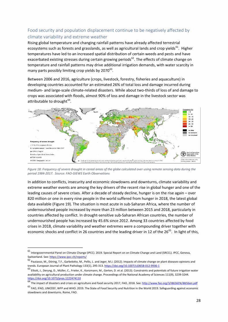
Between 2006 and 2016, agriculture (crops, livestock, forestry, fisheries and aquaculture) in developing countries accounted for an estimated 26% of total loss and damage incurred during medium- and large-scale climate-related disasters. While about two-thirds of loss of and damage to crops was associated with floods, almost 90% of loss and damage in the livestock sector was attributable to drought64.

Figure 18: Frequency of severe drought in cereal areas of the globe calculated over using remote sensing data during the period 1984-2017. Source: FAO-GIEWS Earth Observations

In addition to conflicts, insecurity and economic slowdowns and downturns, climate variability and extreme weather events are among the key drivers of the recent rise in global hunger and one of the leading causes of severe crises. After a decade of steady decline, hunger is on the rise again – over 820 million or one in every nine people in the world suffered from hunger in 2018, the latest global data available (Figure 19). The situation is most acute in sub-Saharan Africa, where the number of undernourished people increased by more than 23 million between 2015 and 2018, particularly in countries affected by conflict. In drought-sensitive sub-Saharan African countries, the number of undernourished people has increased by 45.6% since 2012. Among 33 countries affected by food crises in 2018, climate variability and weather extremes were a compounding driver together with economic shocks and conflict in 26 countries and the leading driver in 12 of the 2665. In light of this,

61 Intergovernmental Panel on Climate Change (IPCC). 2019. Special Report on on Climate Change and Land (SRCCL). IPCC, Geneva, Switzerland. See: https://www.ipcc.ch/reports/ 62 Pautasso, M., Döring, T.F., Garbelotto, M., Pellis, L. and Jeger, M.J. (2012). Impacts of climate change on plant diseases-opinions and trends. European Journal of Plant Pathology 133(1), 295-313. https://doi.org/10.1007/s10658-012-9936-1 63 Elliott, J., Deryng, D., Müller, C., Frieler, K., Konzmann, M., Gerten, D. et al. (2013). Constraints and potentials of future irrigation water availability on agricultural production under climate change. Proceedings of the National Academy of Sciences 111(9), 3239-3244. https://doi.org/10.1073/pnas.1222474110 64 The impact of disasters and crises on agriculture and food security 2017, FAO, 2018. See: http://www.fao.org/3/I8656EN/i8656en.pdf 65 FAO, IFAD, UNICEEF, WFP and WHO. 2019. The State of Food Security and Nutrition in the World 2019. Safeguarding against economic slowdowns and downturns. Rome, FAO.

29

the global community faces an enormous challenge to meet the Zero Hunger target of the 2030 Agenda for Sustainable Development.

Figure 19: Number of undernourished people in the world has been on the rise since 2015, (FAO).

More than 10 million new internal displacements were recorded between January and June 2019. Of these, 7 million were triggered by hydrometeorological events including Cyclone Idai in Southeast Africa, Cyclone Fani in South Asia, Hurricane Dorian in the Caribbean, and flooding in Iran, the Philippines and Ethiopia, generating acute humanitarian and protection needs66. Among natural hazards, floods and storms have contributed the most to displacement recorded so far in 2019, followed by droughts. Asia and the Pacific remain the regions most prone to disaster displacement due to both sudden and slow-onset disasters. For instance, more than 2 million people were evacuated in Bangladesh, the second most disaster-prone country in the region, due to Cyclone Bulbul in November and more than 2 million in China due to Typhoon Lekima in August. Latin America and the Caribbean were also particularly affected by the impacts of climate-related events and other hazards such as volcanic eruptions and earthquakes, resulting in more displacement. For instance, around 70 000 people have become homeless in the Bahamas in September due to hurricane Dorian and more than 42 000 in the Amazonas (Brazil) in June due to flooding67. The number of new displacements associated with weather extremes could more than triple to around 22 million by the end of 201968.

Populations displaced internally and across borders often reside in climate ‘hotspots’, where they are exposed to and affected by slow and sudden-onset hazards, which can result in secondary displacement, among other impacts. For instance, hundreds of thousands of Rohingya refugees who 66 http://www.internal-displacement.org/ http://www.internal-displacement.org/publications/internal-displacement-mid-year-figures-january-june-2019 67 IDMC, http://www.internal-displacement.org/ , 68 Reliefweb, https://reliefweb.int/disasters#content, IDMC, http://www.internal-displacement.org/

30

have fled into Bangladesh and are now residing in Kutupalong are routinely affected by storms and heavy rainfall and landslides. Between January and November 2019, the camps in the area have been hit by floods, landslides and strong winds. Poor building quality and encroachment in exposed areas have resulted in 84 448 people being affected out of a total population of 944 68269.

Although most disaster and climate-related displacement is internal, displacement across borders, which may be interrelated with situations of conflict or violence, also occurs70. The worsening droughts and violence in Somalia drove thousands of people to flee to Ethiopia, a country that also faces adverse impacts from climate-related events. The Lake Chad region has seen desertification, deforestation and drought, associated with the shrinking of Lake Chad, climate events, population growth and unregulated irrigation. Added to violence that has driven millions of people from their homes in Chad, Cameroon, Nigeria and Niger, this exacerbates forced displacement across borders71.

In Southern Africa, the start of the seasonal rains was delayed and there were extensive dry periods. In May 2019, Namibia declared a state of emergency in response to the drought it was facing72. Regional cereal output is forecasted to be about 8 percent below the five-year average with 12.5 million people in the region expected to experience severe food insecurity up to March 2020, an increase of more than 10% from the previous year.

Food security has been deteriorating in several areas of Ethiopia, Somalia, Kenya and Uganda due to a poor long/Gu rainy season, which followed below-average 2018 short/Deyr rains. Overall, about 12.3 million people are food insecure in the Horn of Africa region73. Between October and November 2019, Somalia was further affected by intense flooding that affected 540 000 people, of whom 370 000 were displaced, in Hiran and in parts of Bay, Gedo, Middle Shabelle and Middle Juba regions74.

In March 2019, Tropical Cyclone Idai contributed to complete destruction of close to 780 000 ha of crops in Malawi, Mozambique, and Zimbabwe, further undermining a precarious food security situation in the region75. The cyclone also resulted in at least 50 905 displaced persons in Zimbabwe76, 53 237 in southern Malawi77 and 77 019 in Mozambique78. Mozambique was again hit by Cyclone Kenneth a few weeks later, contributing to a current total of 88 381 IDPs, mostly concentrated in the Beira and Quelimane areas.79

69 http://iom.maps.arcgis.com/apps/MapSeries/index.html?appid=1eec7ad29df742938b6470d77c26575a 70 UNHCR, https://www.unhcr.org/news/stories/2019/10/5da5e18c4/climate-change-and-displacement.html 71 http://www.internal-displacement.org/expert-opinion/looking-beyond-boko-haram-in-the-lake-chad-region, UNHCR, https://www.unhcr.org/news/stories/2019/10/5da5e18c4/climate-change-and-displacement.html 72 AfricaNews (2019-05-06). "Namibia declares national state of emergency over drought". Africanews. 73 FAO. 2019. Early Warning Early Action Report on Food Security an Agriculture (October-December 2019). Rome. 74 https://reliefweb.int/sites/reliefweb.int/files/resources/Situation%20Report%20-%20Somalia%20%20-%2017%20Nov%202019.pdf 75 FAO. 2019. Early Warning Early Action Report on Food Security an Agriculture (July-September 2019). Rome. 76 https://displacement.iom.int/reports/zimbabwe-%E2%80%94-tropical-cyclone-idai-baseline-assessment-round-1-3-27-april-2019?close=true 77 https://displacement.iom.int/reports/malawi-%E2%80%94-tropical-cyclone-idai-multi-sectoral-location-assessments-11-april-2019?close=true 78 https://displacement.iom.int/reports/mozambique-%E2%80%94-cyclone-idai-response-situation-report-%E2%80%94-round-10-october-2019?close=true 79 https://displacement.iom.int/mozambique

31

Food insecurity remained severe in South Sudan throughout 2019 and 5.5 million people are expected80 to be severely food insecure in the first quarter of 2020. More than 1.3 million children are estimated to be acutely malnourished in the country. While favourable rainfall conditions in the second half of the year boosted yields, widespread flash floods affected about 900 000 people and resulted in crop and livestock losses, reversing the gains owing to an improved security situation since late 201881. The flooding also resulted in an increase of water-borne and insect-borne diseases (East Coast Fever, anthrax, and worms)82. In October 2019, unprecedented heavy flooding in South Sudan’s Maban County has affected nearly 200 000 people, including refugees and the host population. The affected area in the Upper Nile State is home to more than 150 000 refugees from Sudan83.

Flash floods in March 2019, following an intense drought from April to October 2018 in Afghanistan, resulted in the worst flooding in a decade in some parts of the country. 13.5 million people are food insecure, with 22 out of 34 provinces still rallying from severe drought conditions faced in 2018, which had already resulted in 32 515 displacements in Herat alone84. The situation is particularly severe because an estimated 80% of soils in the country are degraded due to cumulative years of dry conditions85.

Dry conditions persisted throughout the first half of 2019 in the Democratic People’s Republic of Korea after two consecutive years of dry conditions and irregular weather patterns. On average, only 56.3 mm of rain fell in the country from January to March 2019, which is the lowest on record since 1917. About 10 million people urgently require food assistance86.

In 2019, drier than normal conditions in the “Dry Corridor” of Central America and the Caribbean region led to forest fires across northern Guatemala and Honduras, with a negative impact on crop development and contributing to the drying up of some rivers in Honduras. Due to below normal rainfall from May to August 2019, about 50 000 families lost close to 80% of their maize production in Guatemala. Significant crop losses (up to 70% and 50% for maize and beans, respectively) were also reported in Honduras due to similar dry conditions. In September 2019, the government declared an emergency due to a loss of staple crops with more than 100 000 people at risk of food insecurity. In El Salvador, over 70 000 households are estimated to be affected by a lack of food and safe drinking water87.

80 Methodology used for the calculation is available in page 16 of http://www.ipcinfo.org/fileadmin/user_upload/ipcinfo/docs/IPC_South%20Sudan_Key_Messages_August_2019.pdf 81 FAO, Crop Prospects and Food Situation, December 2019 http://www.fao.org/giews/reports/crop-prospects/en/, https://reliefweb.int/sites/reliefweb.int/files/resources/20191114_south_sudan_floods_emergency_response_strategy_and_funding_requirements.pdf 82 FAO. 2019. Early Warning Early Action Report on Food Security an Agriculture (October-December 2019). Rome. 83 UNHCR, https://www.unhcr.org/news/briefing/2019/10/5da977fe4/unprecedented-flooding-affects-thousands-locals-refugees-south-sudan.html 84 https://displacement.iom.int/reports/afghanistan-%E2%80%94-drought-response-situation-report-26-april-2019?close=true 85 FAO. 2019. Early Warning Early Action Report on Food Security an Agriculture (April-June 2019). Rome. 86 FAO. 2019. Early Warning Early Action Report on Food Security an Agriculture (October-December 2019). Rome. 87 FAO. 2019. Early Warning Early Action Report on Food Security an Agriculture (October-December 2019). Rome.

32

Marine life and biodiversity threatened by the changing climate and extreme events

The ocean is an integral part of the global climate system influencing temperature and rainfall across the planet88,89. The primary pressures on living marine resources are overexploitation, pollution from land-based activities and climate change. Climate change raises ocean temperature, alters ocean circulation, reduces sea-ice extent and thickness, changes salinity, and leads to ocean acidification, sea level rise and changes in extreme weather events90.

Coral reefs are the marine ecosystem most threatened by climate-related ocean change, especially ocean warming and acidification91,92,93. Coral reefs are projected to decline to 10%-30% of former cover at 1.5°C warming, and to less than 1% at 2°C warming94. Ocean acidification may also have negative impacts on other marine systems, including mussel beds and some macroalgal habitats. Fisheries are being affected by climate change in many ways4,95. As temperature and salinity profiles change with global warming, the distribution and productivity of important target species is already being reflected in changes in the distribution of fishery catches.

Recent research based on the long-term monitoring of the Great Barrier Reef (GBR) showed that the hard coral cover increased slightly from 11% in 2017 to 14% in 2019 in the northern GBR. However, these values remain close to the lowest levels recorded by the Australian Institute of Marine Science Long-Term Monitoring Program (AIMS-LTMP) since 1985 due to the cumulative impacts of cyclones and two episodes of severe coral bleaching over the period 2014 to 201996. To date, recovery has been limited.

88 Intergovernmental Panel on Climate Change (IPCC). 2013. Climate Change 2013: The Physical Science Basis. Summary for Policymakers. Cambridge University Press, Cambridge, UK. http://www.ipcc.ch/pdf/ assessment-report/ar5/wg1/WG1AR5_SPM_FINAL.pdf 89 Intergovernmental Panel on Climate Change (IPCC). 2019. Special Report on the Ocean and Cryosphere in a Changing Climate (SROCC). IPCC, Geneva, Switzerland. See: https://www.ipcc.ch/reports/ 90 Salem, H.S. 2011. Social, environmental and security impacts of climate change of the eastern Mediterranean. In: Coping with Global Environmental Change, Disasters and Security – Threats, Challenges, Vulnerabilities and Risks. Brauch, H.S., Spring, U.O., Mesjasz, C., Grin, J., Kameri-Mbote, P., Chourou, B. et al. (eds.). Springer. 421-445. https://www.researchgate.net/publication/299562984_Social_Environmental_and_Security_Impacts_of_Climate_Change_of_the_Eastern_Mediterranian 91 Gattuso, J.P., Magnan, A., Billé, R., Cheung, W.W., Howes, E.L., Joos, F., Allemand, D., Bopp, L., Cooley, S.R., Eakin, C.M. and Hoegh-Guldberg, O., 2015. Contrasting futures for ocean and society from different anthropogenic CO2 emissions scenarios. Science, 349(6243), p.aac4722. 92 Albright R, Takeshita Y, Koweek DA, Ninokawa A, Wolfe K, Rivlin T, et al. (2018) Carbon dioxide addition to coral reef waters suppresses net community calcification. Nature, 555, 516–519. 93 Hoegh-Guldberg, O. et al., 2018: Impacts of 1.5 ºC global warming on natural and human systems. In: Global Warming of 1.5°C. An IPCC Special Report on the impacts of global warming of 1.5°C above pre-industrial levels and related global greenhouse gas emission pathways, in the context of strengthening the global response to the threat of climate change, sustainable development, and efforts to eradicate poverty [Masson-Delmotte, V., P. Zhai, H.-O. Pörtner, D. Roberts, J. Skea, P. R. Shukla, A. Pirani, W. Moufouma-Okia, C. Péan, R. Pidcock, S. Connors, J. B. R. Matthews, Y. Chen, X. Zhou, M. I. Gomis, E. Lonnoy, T. Maycock, M. Tignor and T. Waterfield (eds.)]. In press. 94 Intergovernmental Science-Policy Platform on Biodiversity and Ecosystem Services (IPBES). 2019. Global Assessment on Biodiversity and Ecosystem Services – Summary for Policy-Makers. Bonn, Germany. https://www.ipbes.net/news/ipbes-global-assessment-summary-policymakers-pdf 95 Ripple, W., C. Wolf, T.M. Newsome, P. Barnard and W.R. Moomaw. 2019. World Scientists’ Warning of a Climate Emergency. BioScience, biz088, https://doi.org/10.1093/biosci/biz088 96 AIMS Long-term Reef Monitoring Program - Annual Summary Report on coral reef condition for 2018/19 [Available here: https://www.aims.gov.au/reef-monitoring/gbr-condition-summary-2018-2019].

33

Figure 20: Trends in average hard coral cover for the Northern GBR based on manta tow surveys to June 2019. N indicates the number of reefs contributing to the analyses; blue shading represents 95% credible intervals. Note that many reefs in this region do not have a regular survey history and that in 2019, not all inshore reefs could be surveyed (AIMS, 2019)97.

Severe Tropical Cyclone (STC) Debbie in 2017, and continued southward spread of crown-of-thorns starfish outbreaks, contributed to a continuing decrease of coral cover in the reefs in the Central GBR. Average hard coral cover declined slightly, from 14% in 2018 to 12% in 2019. Overall, mean coral cover on reefs in the Southern GBR region continued to decline, albeit only slightly, from 25% in 2018 to 24% in 2019.

Full list of contributors Physical aspects Anny Cazanave (Laboratoire d’Etudes en Géophysique et Océanographie Spatiales CNES and Observatoire Midi-Pyrénées, France), Robert Dunn (UK Met Office), Karsten Haustein (Oxford University, UK), Kirsten Isensee (Intergovernmental Oceanographic Commission of the United Nations Educational, Scientific and Cultural Organization), John Kennedy (Met Office, UK), Rachel Killick (Met Office, UK), Jennifer Howard (Conservation International), Lisa Levin (Scripps), Patrick Megonigal (Smithsonian Environmental Research Center), Robert W Schlegel (Department of Physical Oceanography, Woods Hole Oceanographic Institution, US), Katherina Luise Schoo (Intergovernmental Oceanographic Commission of the United Nations Educational Scientific and Cultural Organization), Karina von Schuckmann (Mercator Océan International, France), Vasily Smolyanitsky (Arctic and Antarctic Research Institute, Russian Federation), Martin Stendel (Danish Meteorological Institute, Denmark), Oksana Tarasova (GAW WMO), Blair Trewin (Bureau of Meteorology, Australia), Freja Vamborg (ECMWF and C3S), Michael Zemp (Switzerland), Markus Ziese (Deutscher Wetterdienst, Germany).

Climate related risks and impacts Pierre Boileau (UNEP), Alessandro Costantino (FAO), Florence Geoffroy (UNHCR), Sarah Graf (FAO), Lorenzo Guadagno (IOM), Dina Ionesco (IOM), Kirsten Isensee (IOC-UNESCO), Maarten Kappelle

97 AIMS Long-term Reef Monitoring Program - Annual Summary Report on coral reef condition for 2018/19 [Available here: https://www.aims.gov.au/reef-monitoring/gbr-condition-summary-2018-2019].

34

(UNEP), Isabelle Michal (UNHCR), Lev Neretin (FAO), Oscar Rojas (FAO), Pinya Sarasas (UNEP), Jeremy Schlickenrieder (FAO), Joy Shumake-Guillemot (WHO/WMO), Yanchun Zhang (UNCTAD)

Also contributed Sandra Amlang (UNDRR), Diarmid Campbell Lendrum (WHO), Pep Canadell (CSIRO), Katherine Hill (GCOS/GOOS), Clare Nullis (WMO), Wilfran Moufouma Okia (WMO), Mxolisi Shongwe (IPCC Secretariat), Michael Sparrow (WCRP), Zinta Zommers (UNDRR).

Agencies World Meteorological Organisation (WMO), Food and Agriculture Organization of the United Nations (FAO), United Nations Environment Programme (UNEP), and the Intergovernmental Oceanographic Commission of the United Nations Educational, Scientific and Cultural Organization (IOC - UNESCO), United Nations High Commissioner for Refugees (UNHCR), International Organization for Migration (IOM), United Nations Conference on Trade and Development (UNCTAD), World Health Organisation (WHO), United Nations Office for Disaster Risk Reduction (UNDRR). Country contributions

Algeria, Argentina, Armenia, Austria, Bangladesh, Bulgaria, Cameroon, Canada, Chile, China, Costa Rica, Côte d’Ivoire, Croatia, Cyprus, Denmark, Estonia, Finland, France, Georgia, Germany, Greece, Guinea, India, Indonesia, Iran, Ireland, Israel, Italy, Japan, Jordan, Kazakhstan, Kenya, Latvia, Libya, Luxembourg, Republic of North Macedonia, Malaysia, Moldova, Morocco, Netherlands, New Zealand, Nigeria, Philippines, Poland, Senegal, Serbia, Singapore, Slovakia, Slovenia, South Africa, Spain, Sudan, Sweden, Switzerland, Tajikistan, Tanzania, Trinidad and Tobago, Tunisia, Turkey, Ukraine, United Kingdom, USA.

Data Global Precipitation Climatology Centre (Deutscher Wetterdienst, Germany), Met Office Hadley Centre (UK), National Oceanic and Atmospheric Administration National Centres for Environmental Information, European Centre for Medium-range Weather Forecasts and Copernicus Climate Change Service, National Aeronautics and Space Administration Goddard Institute for Space Studies, Japan Meteorological Agency, WMO Global Atmospheric Watch, NOAA National Ocean Data Center, National Snow and Ice Data Center, Mauna Loa Observatory, the Blue Carbon Initiative, the Global Ocean Oxygen Network, the Global Ocean Acidification Observing Network, Hong Kong Observatory, Pan-Arctic Regional Climate Outlook Forum, European Space Agency Climate Change Initiative, Copernicus Marine Environmental Monitoring Service and AVISO (Archiving, Validation and Interpretation of Satellite Oceanographic data), Polar Portal, Department of Physical Oceanography, Woods Hole Oceanographic Institution, AARI Arctic and Antarctic Research Institute, Mercator Ocean, IOC - Global Ocean Oxygen Network (GO2NE), Global Ocean Acidification Observing Network (GOA-ON).