Wireless Communication FundamentalsWireless Communication Fundamentals

David TipperAssociate ProfessorAssociate Professor

Graduate Telecommunications and Networking Program

U i it f Pitt b hUniversity of PittsburghTelcomTelcom 2700 Slides 22700 Slides 2

Wireless NetworksWireless Networks

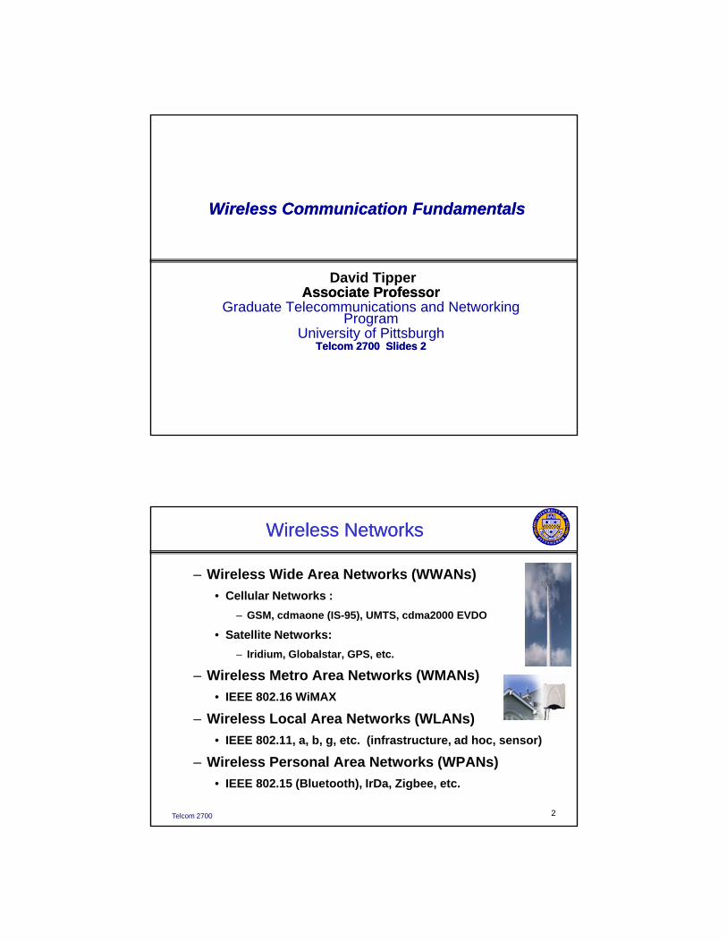
– Wireless Wide Area Networks (WWANs)

• Cellular Networks :

GSM d (IS 95) UMTS d 2000 EVDO– GSM, cdmaone (IS-95), UMTS, cdma2000 EVDO

• Satellite Networks:

– Iridium, Globalstar, GPS, etc.

– Wireless Metro Area Networks (WMANs)

• IEEE 802.16 WiMAX

– Wireless Local Area Networks (WLANs)

Telcom 2700 2

– Wireless Local Area Networks (WLANs)

• IEEE 802.11, a, b, g, etc. (infrastructure, ad hoc, sensor)

– Wireless Personal Area Networks (WPANs)

• IEEE 802.15 (Bluetooth), IrDa, Zigbee, etc.

Wireless Issues

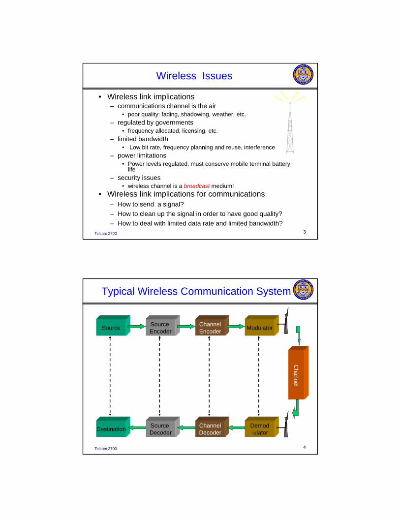
• Wireless link implications– communications channel is the air

• poor quality: fading, shadowing, weather, etc.

regulated by governments– regulated by governments• frequency allocated, licensing, etc.

– limited bandwidth • Low bit rate, frequency planning and reuse, interference

– power limitations• Power levels regulated, must conserve mobile terminal battery

life

– security issues

Telcom 2700 3

y• wireless channel is a broadcast medium!

• Wireless link implications for communications– How to send a signal?

– How to clean up the signal in order to have good quality?

– How to deal with limited data rate and limited bandwidth?

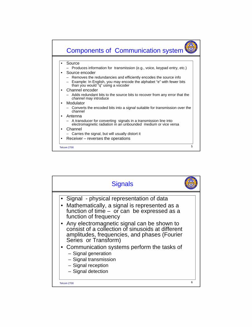
Typical Wireless Communication System

SourceSource Encoder

ChannelEncoder

Modulator

Channel

Telcom 2700 4

DestinationSource Decoder

ChannelDecoder

Demod-ulator

Components of Communication system

• Source– Produces information for transmission (e.g., voice, keypad entry, etc.)

• Source encoderRemoves the redundancies and efficiently encodes the source info– Removes the redundancies and efficiently encodes the source info

– Example: In English, you may encode the alphabet “e” with fewer bits than you would “q” using a vocoder

• Channel encoder– Adds redundant bits to the source bits to recover from any error that the

channel may introduce• Modulator

– Converts the encoded bits into a signal suitable for transmission over the channel

Telcom 2700 5

• Antenna– A transducer for converting signals in a transmission line into

electromagnetic radiation in an unbounded medium or vice versa• Channel

– Carries the signal, but will usually distort it• Receiver – reverses the operations

Signals

• Signal - physical representation of data• Mathematically, a signal is represented as a

function of time – or can be expressed as afunction of time or can be expressed as a function of frequency

• Any electromagnetic signal can be shown to consist of a collection of sinusoids at different amplitudes, frequencies, and phases (Fourier Series or Transform)

• Communication systems perform the tasks of

Telcom 2700 6

y p– Signal generation– Signal transmission– Signal reception– Signal detection

Terminology

• Consider a periodic signal (e.g., a sine wave)• Period (T) - amount of time it takes for one repetition of

the signalthe signalT = 1/frequency = 1/f

• Phase () - measure of the relative position in time within a single period of the signal

• Wavelength () - distance occupied by a single cycle of the signal– Or, the distance between two points of corresponding phase of

Telcom 2700 7

, p p g ptwo consecutive cycles

• For electromagnetic waves in air or free space, = c/fwhere c is the speed of light = 3 x 108 m/sec

Consider a Sinusoid

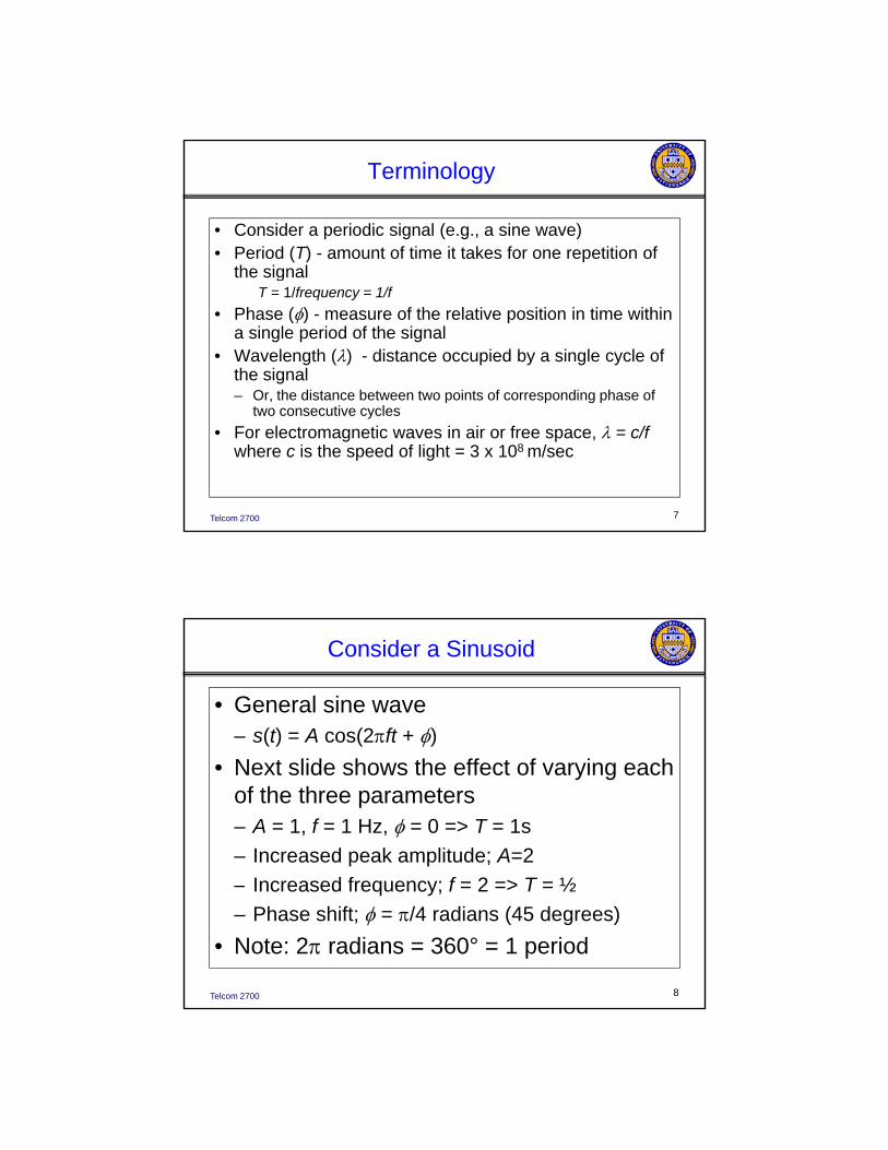
• General sine wave– s(t) = A cos(2ft + )

• Next slide shows the effect of varying each of the three parameters– A = 1, f = 1 Hz, = 0 => T = 1s

– Increased peak amplitude; A=2

I d f f 2 T ½

Telcom 2700 8

– Increased frequency; f = 2 => T = ½

– Phase shift; = /4 radians (45 degrees)

• Note: 2 radians = 360° = 1 period

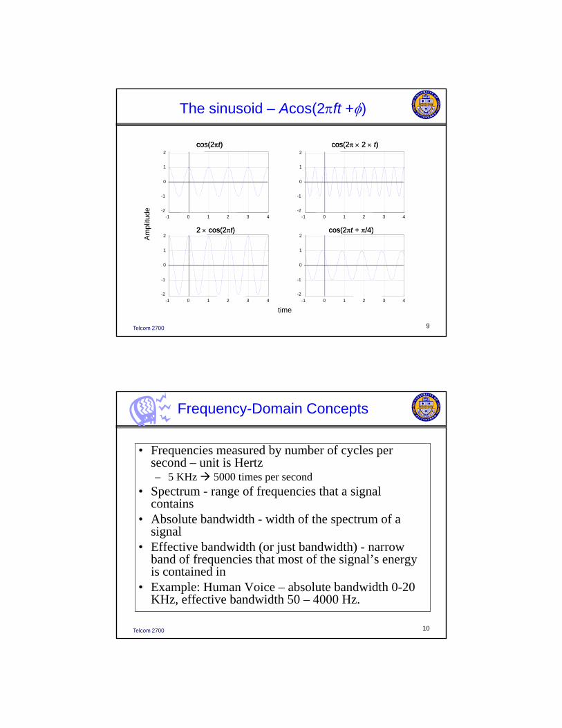
The sinusoid – Acos(2ft +)

1

2

1

2

cos(2cos(2tt)) cos(2cos(2 2 2 tt))

-1 0 1 2 3 4-2

-1

0

-1 0 1 2 3 4-2

-1

0

1

2

1

22 2 cos(2cos(2tt)) cos(2cos(2tt + + /4)/4)

Am

plitu

de

Telcom 2700 9

-1 0 1 2 3 4

-2

-1

0

-1 0 1 2 3 4

-2

-1

0

time

Frequency-Domain Concepts

• Frequencies measured by number of cycles per second – unit is Hertz

5 KH 5000 i d– 5 KHz 5000 times per second • Spectrum - range of frequencies that a signal

contains• Absolute bandwidth - width of the spectrum of a

signal• Effective bandwidth (or just bandwidth) - narrow

b d f f i th t t f th i l’

Telcom 2700 10

band of frequencies that most of the signal’s energy is contained in

• Example: Human Voice – absolute bandwidth 0-20 KHz, effective bandwidth 50 – 4000 Hz.

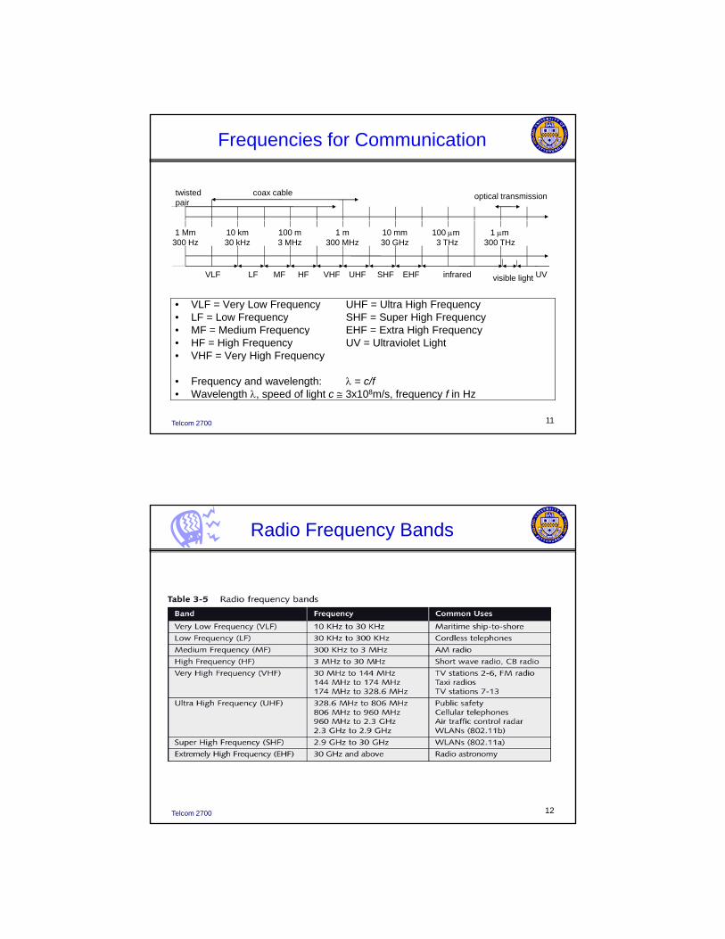
Frequencies for Communication

optical transmissioncoax cabletwisted pair

• VLF = Very Low Frequency UHF = Ultra High Frequency• LF = Low Frequency SHF = Super High Frequency

MF M di F EHF E t Hi h F

1 Mm300 Hz

10 km30 kHz

100 m3 MHz

1 m300 MHz

10 mm30 GHz

100 m3 THz

1 m300 THz

visible lightVLF LF MF HF VHF UHF SHF EHF infrared UV

Telcom 2700 11

• MF = Medium Frequency EHF = Extra High Frequency• HF = High Frequency UV = Ultraviolet Light• VHF = Very High Frequency

• Frequency and wavelength: = c/f• Wavelength , speed of light c 3x108m/s, frequency f in Hz

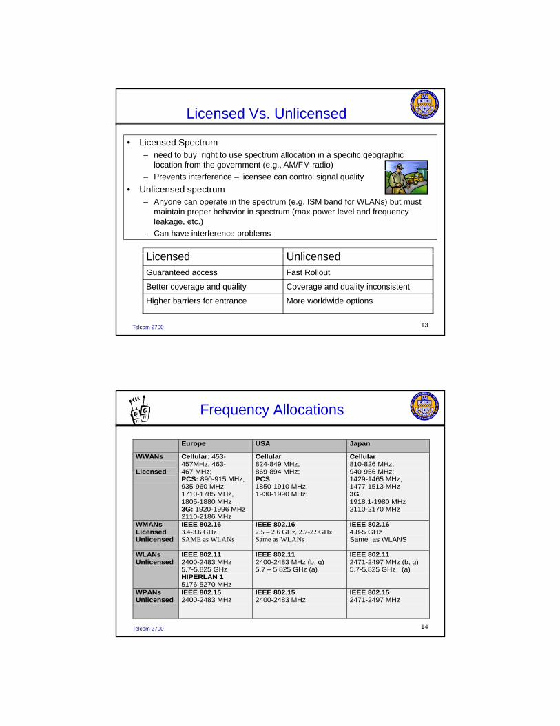
Radio Frequency Bands

Telcom 2700 12

Licensed Vs. Unlicensed

• Licensed Spectrum– need to buy right to use spectrum allocation in a specific geographic

location from the government (e.g., AM/FM radio)

Li d U li d

– Prevents interference – licensee can control signal quality

• Unlicensed spectrum – Anyone can operate in the spectrum (e.g. ISM band for WLANs) but must

maintain proper behavior in spectrum (max power level and frequency leakage, etc.)

– Can have interference problems

Telcom 2700 13

Licensed UnlicensedGuaranteed access Fast Rollout

Better coverage and quality Coverage and quality inconsistent

Higher barriers for entrance More worldwide options

Frequency Allocations

Europe USA Japan

WWANs Licensed

Cellular: 453-457MHz, 463-467 MHz;

Cellular 824-849 MHz, 869-894 MHz;

Cellular 810-826 MHz, 940-956 MHz;Licensed

467 MHz; PCS: 890-915 MHz, 935-960 MHz; 1710-1785 MHz, 1805-1880 MHz 3G: 1920-1996 MHz 2110-2186 MHz

869-894 MHz;PCS 1850-1910 MHz, 1930-1990 MHz;

940-956 MHz; 1429-1465 MHz, 1477-1513 MHz 3G 1918.1-1980 MHz 2110-2170 MHz

WMANs Licensed Unlicensed

IEEE 802.16 3.4-3.6 GHz SAME as WLANs

IEEE 802.16 2.5 – 2.6 GHz, 2.7-2.9GHz Same as WLANs

IEEE 802.16 4.8-5 GHz Same as WLANS

WLANs IEEE 802 11 IEEE 802 11 IEEE 802 11

Telcom 2700 14

WLANs Unlicensed

IEEE 802.11 2400-2483 MHz 5.7-5.825 GHz HIPERLAN 1 5176-5270 MHz

IEEE 802.11 2400-2483 MHz (b, g) 5.7 – 5.825 GHz (a)

IEEE 802.112471-2497 MHz (b, g) 5.7-5.825 GHz (a)

WPANs Unlicensed

IEEE 802.15 2400-2483 MHz

IEEE 802.15 2400-2483 MHz

IEEE 802.15 2471-2497 MHz

What is Signal Propagation?

• Signal Propagation describes how a radio signal is transformed from the time it leaves a transmitter to the time it reaches the receiver

• Important for the design, operation and analysis of wireless networks– Where should transmitters (i.e., base stations/access points)

be placed– What transmit powers should be used– What frequency channels need be assigned to a transmitter– How are handoff decision algorithms affected…

Telcom 2700

• Propagation in free open space like light rays• In general make analogy to light and sound waves

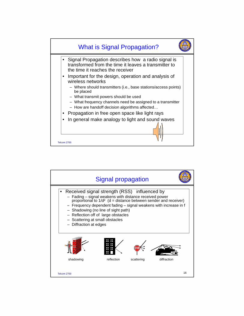
Signal propagation

• Received signal strength (RSS) influenced by– Fading – signal weakens with distance received power

proportional to 1/d² (d = distance between sender and receiver)– Frequency dependent fading – signal weakens with increase in f– Frequency dependent fading – signal weakens with increase in f– Shadowing (no line of sight path)– Reflection off of large obstacles– Scattering at small obstacles– Diffraction at edges

Telcom 2700 16

reflection scattering diffractionshadowing

Signal Propagation

• Effects are similar indoors and out• Several paths from Tx to Rx

– Different delays, phases and amplitudesamplitudes

– Add motion – makes it very complicated

• Termed a multi-path propagationenvironment

• Difficult to look at all of the effects in a composite way

• In practice Transmission Diffraction

Tx

Telcom 2700 17

– Ray Tracing Approach: Breakdown phenomena into different categories use physics model for each path

– Use empirical based models

Reflection

Scattering

Rx

Multipath Propagation

• Signal can take many different paths between sender and receiver due to reflection, scattering, diffraction

signal at sendersignal at receiver

• Time dispersion: signal is dispersed over time

Telcom 2700 18

• interference with “neighbor” symbols, Inter Symbol Interference (ISI)

• The signal reaches a receiver directly and phase shifted• distorted signal depending on the phases of the different

parts• Limits the data rate on the channel

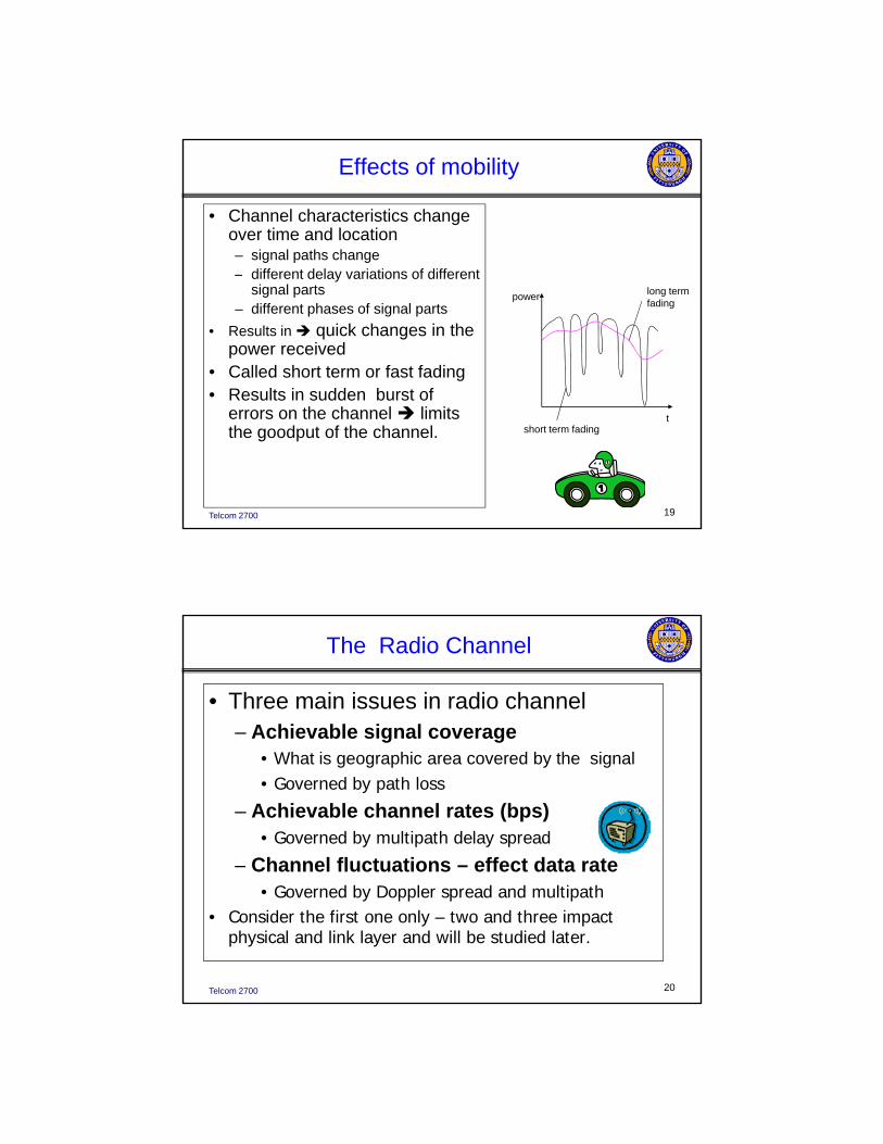
Effects of mobility

• Channel characteristics change over time and location – signal paths change

diff t d l i ti f diff t– different delay variations of different signal parts

– different phases of signal parts

• Results in quick changes in the power received

• Called short term or fast fading• Results in sudden burst of

long termfading

power

Telcom 2700 19

Results in sudden burst of errors on the channel limits the goodput of the channel. short term fading

t

The Radio Channel

• Three main issues in radio channel– Achievable signal coverage

• What is geographic area covered by the signal

• Governed by path loss

– Achievable channel rates (bps)• Governed by multipath delay spread

– Channel fluctuations – effect data rate

Telcom 2700 20

• Governed by Doppler spread and multipath• Consider the first one only – two and three impact

physical and link layer and will be studied later.

Coverage

• Determines– Transmit power required to provide service in a given area

(link budget)– Interference from other transmitters– Interference from other transmitters– Number of base stations or access points that are required

• Parameters of importance (Large Scale/Term Fading effects)– Path loss (long term fading)– Shadow fading

Telcom 2700 21

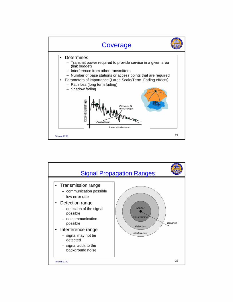
Signal Propagation Ranges

• Transmission range– communication possible

low error rate

distance

sender

transmission

detection

– low error rate

• Detection range– detection of the signal

possible

– no communication possible

• Interference range

Telcom 2700 22

interferenceInterference range– signal may not be

detected

– signal adds to the background noise

Decibels

• Power (signal strength) is expressed in decibels (dB) for ease of calculation– Values relative to 1 mW are expressed in dBm

• Power in dBm = log10 (Power in W / 1 mW)Power in dBm log10 (Power in W / 1 mW) – Values relative to 1 W are expressed in dBW

• Power in dBW = log10 (Power in W / 1 W) – Other values are simply expressed in dB (i.e., Gains of

Antennas, loss due to obstacles, etc.)

• Example 1: Express 2 W in dBm and dBW– dBm: 10 log10 (2 W / 1 mW) = 10 log10(2000) = 33 dBm

Telcom 2700 23

– dBW: 10 log10 (2 W / 1 W) = 10 log10(2) = 3 dBW

• In general dBm value = 30 + dBW value• Note 3 dB implies doubling/halving power

Free Space Loss Model

• Assumptions– Transmitter and receiver are in free open space– No obstructing objects in between– The earth is at an infinite distance!

The transmitted power is P– The transmitted power is Pt

– The received power is Pr

– Isotropic antennas • Antennas radiate and receive equally in all directions with unit gain

• The path loss is the difference between the received signal strength and the transmitted signal strength

PL = Pt (dB) – Pr (dB)

Telcom 2700 24

d

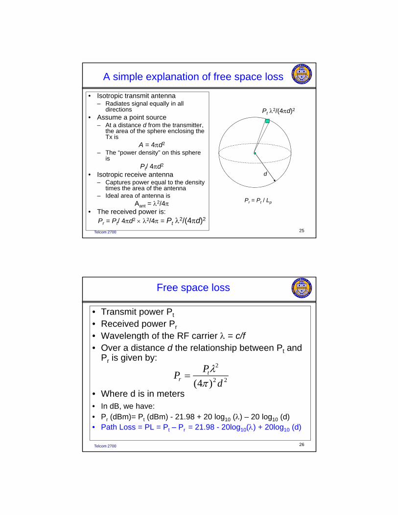
A simple explanation of free space loss

• Isotropic transmit antenna– Radiates signal equally in all

directions• Assume a point source

Pt 2/(4d)2

– At a distance d from the transmitter, the area of the sphere enclosing the Tx is

A = 4d2

– The “power density” on this sphere is

Pt/ 4d2

• Isotropic receive antenna d

Telcom 2700 25

– Captures power equal to the density times the area of the antenna

– Ideal area of antenna isAant = 2/4

• The received power is:Pr = Pt/ 4d2 2/4 = Pt 2/(4d)2

Pr = Pt / Lp

Free space loss

• Transmit power Pt

• Received power Pr

• Wavelength of the RF carrier = c/f• Wavelength of the RF carrier = c/f• Over a distance d the relationship between Pt and

Pr is given by:

• Where d is in meters

22

2

)4( d

PP t

r

Telcom 2700 26

• Where d is in meters• In dB, we have:• Pr (dBm)= Pt (dBm) - 21.98 + 20 log10 () – 20 log10 (d)• Path Loss = PL = Pt – Pr = 21.98 - 20log10() + 20log10 (d)

Free Space Propagation

• Notice that factor of 10 increase in distance => 20 dB increase in path loss (20 dB/decade)( )

Distance Path Loss at 880 MHz 1km 91.29 dB 10Km 111.29 dB

• Note that higher the frequency the greater the path loss for a fixed distance

Telcom 2700 27

Distance 880 MHz 1960MHz1km 91.29 dB 98.25 dBthus 7 dB greater path loss for PCS band compared to cellular band in the US

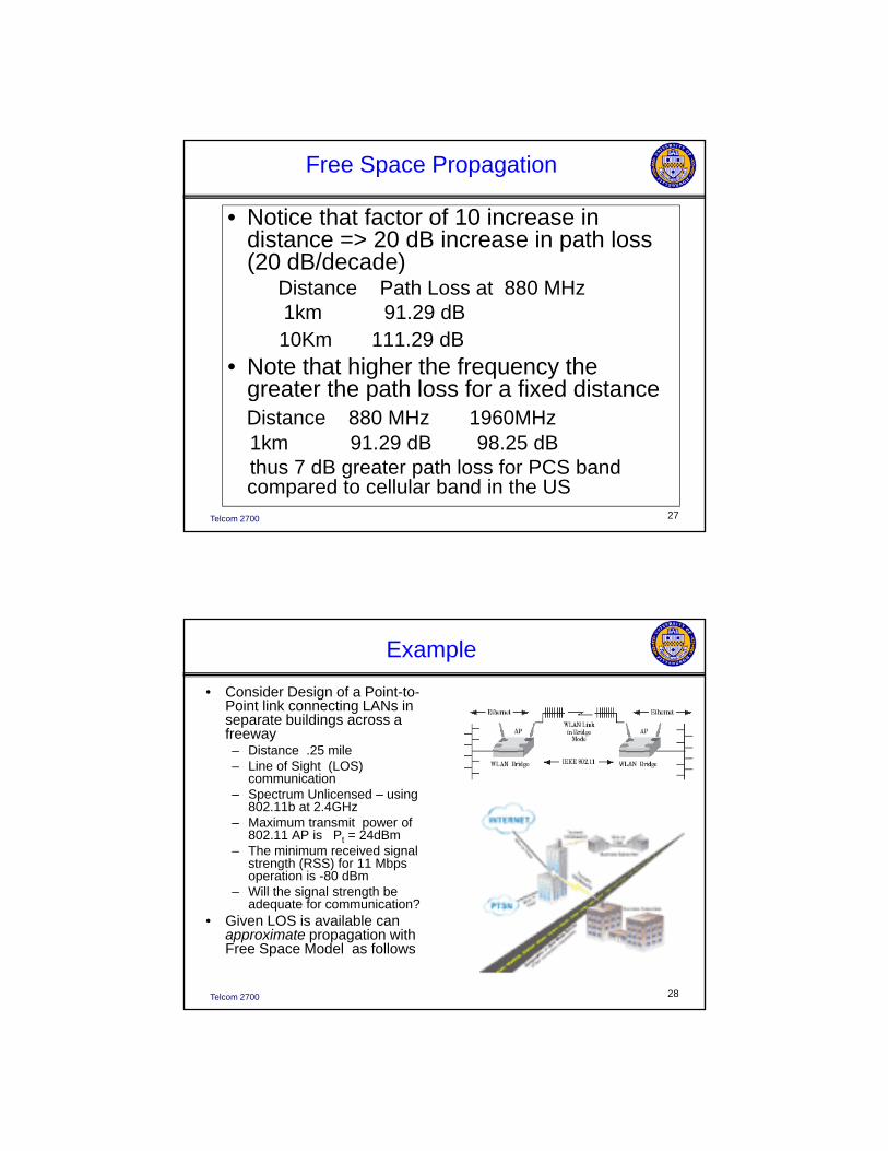
Example

• Consider Design of a Point-to-Point link connecting LANs in separate buildings across a freeway

Distance 25 mile– Distance .25 mile– Line of Sight (LOS)

communication – Spectrum Unlicensed – using

802.11b at 2.4GHz– Maximum transmit power of

802.11 AP is Pt = 24dBm – The minimum received signal

strength (RSS) for 11 Mbps operation is -80 dBm

Telcom 2700 28

operation is 80 dBm– Will the signal strength be

adequate for communication?• Given LOS is available can

approximate propagation with Free Space Model as follows

Example

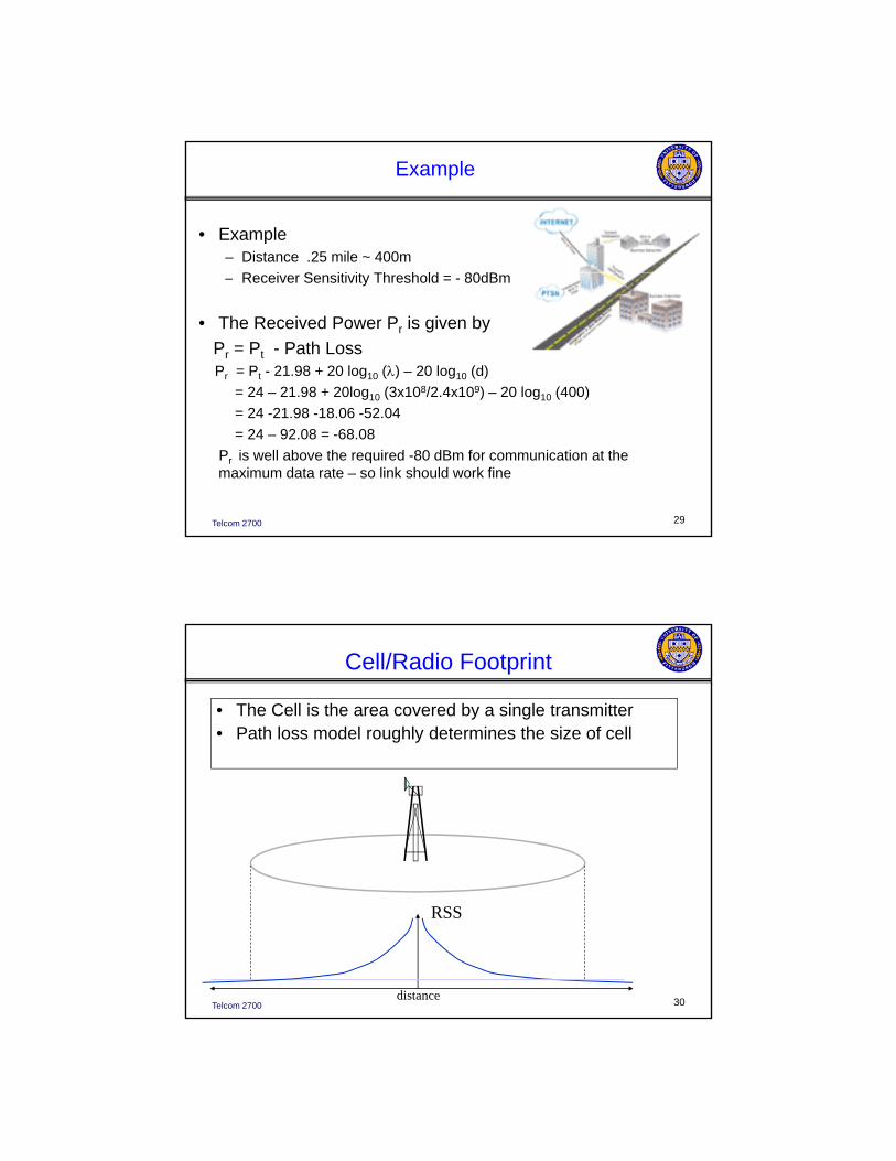
• Example – Distance .25 mile ~ 400m

R i S iti it Th h ld 80dB– Receiver Sensitivity Threshold = - 80dBm

• The Received Power Pr is given by

Pr = Pt - Path LossPr = Pt - 21.98 + 20 log10 () – 20 log10 (d)

= 24 – 21.98 + 20log10 (3x108/2.4x109) – 20 log10 (400)

Telcom 2700 29

= 24 -21.98 -18.06 -52.04

= 24 – 92.08 = -68.08

Pr is well above the required -80 dBm for communication at the maximum data rate – so link should work fine

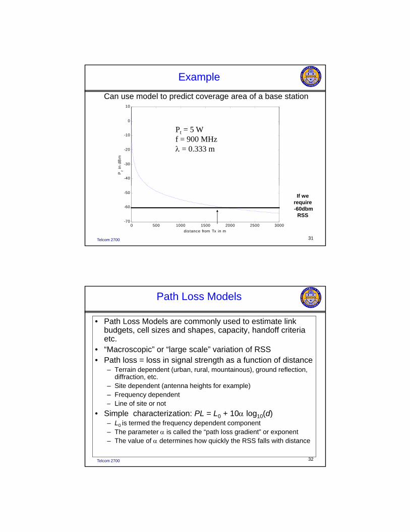
Cell/Radio Footprint

• The Cell is the area covered by a single transmitter• Path loss model roughly determines the size of cell

Telcom 2700 30

RSS

distance

0

10

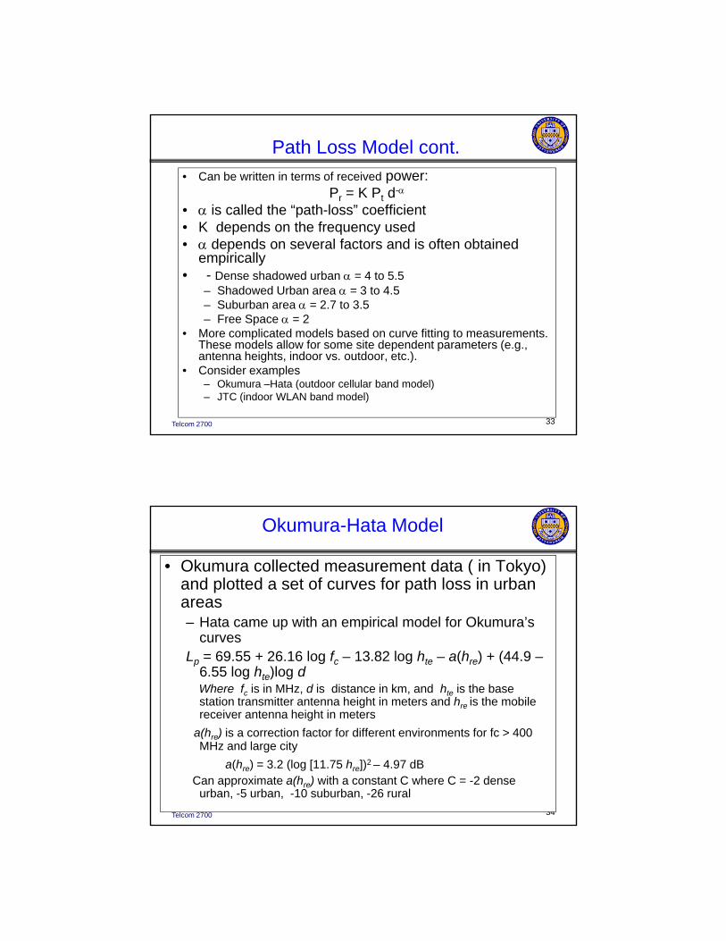
Example

Can use model to predict coverage area of a base station

-40

-30

-20

-10

Pr i

n d

Bm

Pt = 5 Wf = 900 MHz = 0.333 m

Telcom 2700 31

0 500 1000 1500 2000 2500 3000-70

-60

-50

distance from Tx in m

If we require-60dbm

RSS

Path Loss Models

• Path Loss Models are commonly used to estimate link budgets, cell sizes and shapes, capacity, handoff criteria etc.

• “Macroscopic” or “large scale” variation of RSS• Path loss = loss in signal strength as a function of distance

– Terrain dependent (urban, rural, mountainous), ground reflection, diffraction, etc.

– Site dependent (antenna heights for example)– Frequency dependent– Line of site or not

Telcom 2700 32

• Simple characterization: PL = L0 + 10 log10(d)– L0 is termed the frequency dependent component– The parameter is called the “path loss gradient” or exponent– The value of determines how quickly the RSS falls with distance

Path Loss Model cont.

• Can be written in terms of received power:Pr = K Pt d-

• is called the “path-loss” coefficient• K depends on the frequency used • depends on several factors and is often obtained

empirically• - Dense shadowed urban = 4 to 5.5

– Shadowed Urban area = 3 to 4.5– Suburban area = 2.7 to 3.5– Free Space = 2

Telcom 2700 33

• More complicated models based on curve fitting to measurements. These models allow for some site dependent parameters (e.g., antenna heights, indoor vs. outdoor, etc.).

• Consider examples – Okumura –Hata (outdoor cellular band model)– JTC (indoor WLAN band model)

Okumura-Hata Model

• Okumura collected measurement data ( in Tokyo) and plotted a set of curves for path loss in urban areas– Hata came up with an empirical model for Okumura’s

curvesLp = 69.55 + 26.16 log fc – 13.82 log hte – a(hre) + (44.9 –

6.55 log hte)log dWhere fc is in MHz, d is distance in km, and hte is the base station transmitter antenna height in meters and hre is the mobile receiver antenna height in meters

Telcom 2700 34

g

a(hre) is a correction factor for different environments for fc > 400 MHz and large city

a(hre) = 3.2 (log [11.75 hre])2 – 4.97 dBCan approximate a(hre) with a constant C where C = -2 dense

urban, -5 urban, -10 suburban, -26 rural

Example of Hata’s Model

• Consider the case where hre = 2 m receiver antenna’s heighthte = 100 m transmitter antenna’s heightte gfc = 900 MHz carrier frequency

• Lp = 118.14 + 31.8 log d– The path loss exponent for this particular case is =

3.18• What is the path loss at d = 5 km?

– d = 5 km Lp = 118.14 + 31.8 log 5 = 140.36 dB

Telcom 2700 35

p

• If the maximum allowed path loss is 120 dB, what distance can the signal travel?– Lp = 120 = 118.14 + 31.8 log d => d =

10(1.86/31.8) = 1.14 km

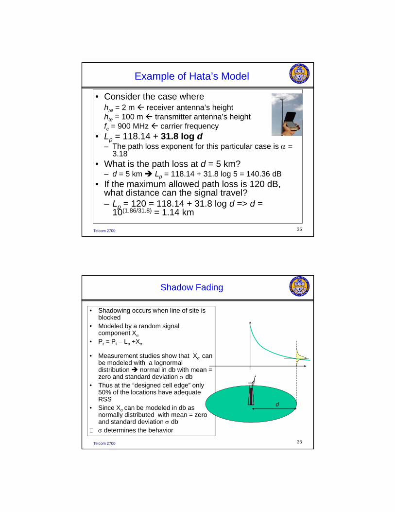
Shadow Fading

• Shadowing occurs when line of site is blocked

• Modeled by a random signal component Xcomponent X

• Pr = Pt – Lp +X

• Measurement studies show that Xcan be modeled with a lognormal distribution normal in db with mean = zero and standard deviation db

• Thus at the “designed cell edge” only 50% of the locations have adequate

Telcom 2700 36

50% of the locations have adequate RSS

• Since Xcan be modeled in db as normally distributed with mean = zero and standard deviation db determines the behavior

d

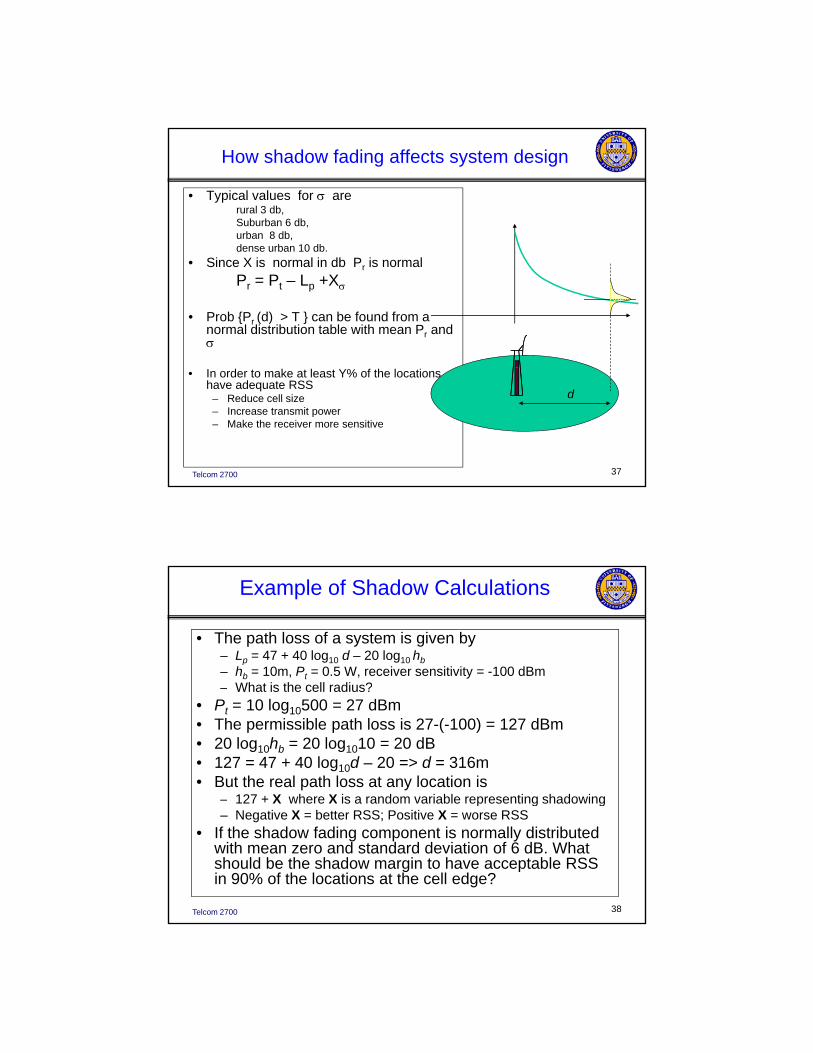
How shadow fading affects system design

• Typical values for are rural 3 db, Suburban 6 db, urban 8 db, dense urban 10 dbdense urban 10 db.

• Since X is normal in db Pr is normal

Pr = Pt – Lp +X

• Prob {Pr (d) > T } can be found from a normal distribution table with mean Pr and

Telcom 2700 37

• In order to make at least Y% of the locations have adequate RSS

– Reduce cell size– Increase transmit power– Make the receiver more sensitive

d

Example of Shadow Calculations

• The path loss of a system is given by– Lp = 47 + 40 log10 d – 20 log10 hb

– hb = 10m, Pt = 0.5 W, receiver sensitivity = -100 dBmWhat is the cell radius?– What is the cell radius?

• Pt = 10 log10500 = 27 dBm• The permissible path loss is 27-(-100) = 127 dBm• 20 log10hb = 20 log1010 = 20 dB• 127 = 47 + 40 log10d – 20 => d = 316m• But the real path loss at any location is

– 127 + X where X is a random variable representing shadowing

Telcom 2700 38

p g g– Negative X = better RSS; Positive X = worse RSS

• If the shadow fading component is normally distributed with mean zero and standard deviation of 6 dB. What should be the shadow margin to have acceptable RSS in 90% of the locations at the cell edge?

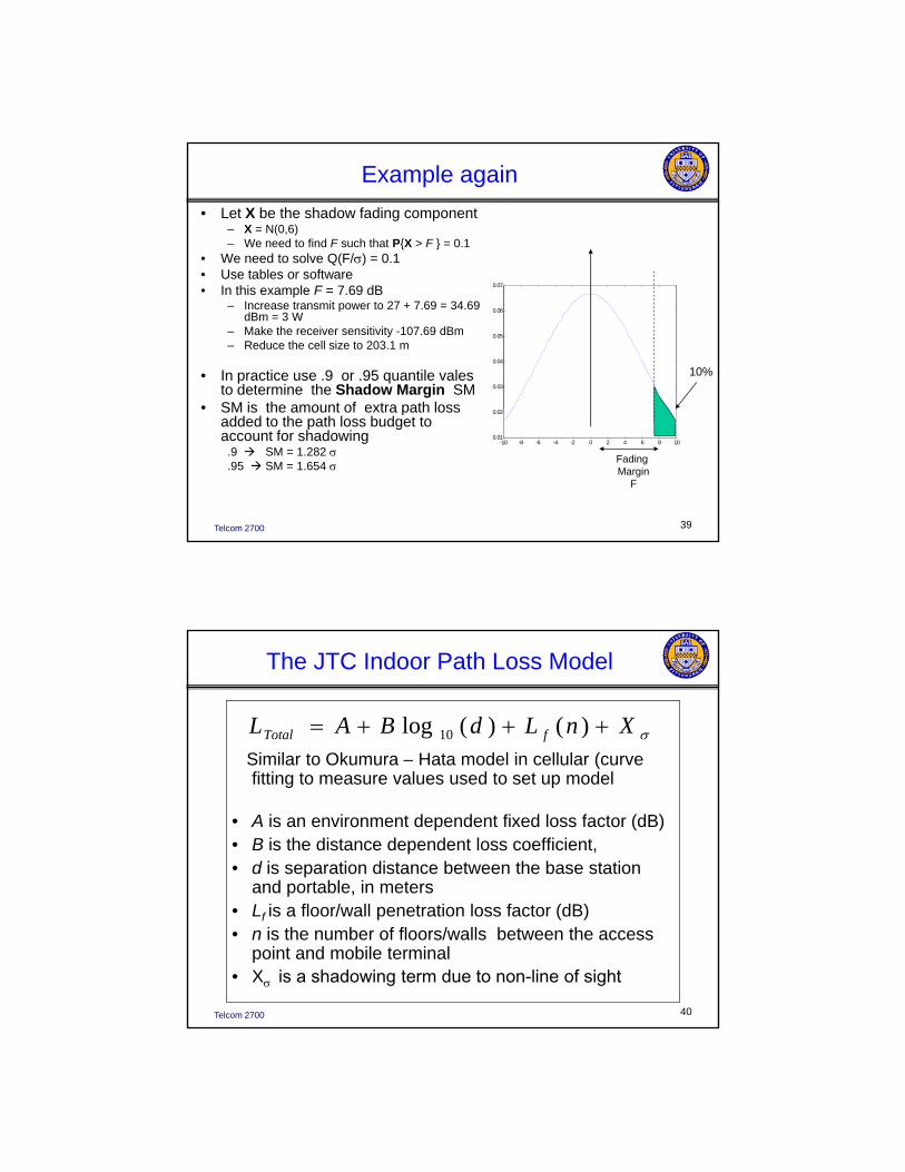
Example again

• Let X be the shadow fading component– X = N(0,6)– We need to find F such that P{X > F } = 0.1

• We need to solve Q(F/) = 0.1• Use tables or software• Use tables or software• In this example F = 7.69 dB

– Increase transmit power to 27 + 7.69 = 34.69 dBm = 3 W

– Make the receiver sensitivity -107.69 dBm– Reduce the cell size to 203.1 m

• In practice use .9 or .95 quantile vales to determine the Shadow Margin SM

• SM is the amount of extra path loss

0.03

0.04

0.05

0.06

0.07

10%

Telcom 2700 39

• SM is the amount of extra path loss added to the path loss budget to account for shadowing

.9 SM = 1.282

.95 SM = 1.654

-10 -8 -6 -4 -2 0 2 4 6 8 100.01

0.02

Fading Margin

F

The JTC Indoor Path Loss Model

Similar to Okumura – Hata model in cellular (curve

XnLdBAL fTotal )()(log 10

Similar to Okumura Hata model in cellular (curve fitting to measure values used to set up model

• A is an environment dependent fixed loss factor (dB)• B is the distance dependent loss coefficient,• d is separation distance between the base station

and portable, in meters

Telcom 2700 40

p• Lf is a floor/wall penetration loss factor (dB)• n is the number of floors/walls between the access

point and mobile terminal• X is a shadowing term due to non-line of sight

JTC Model (Continued)

Environment Residential Office Commercial

A (dB) 38 38 38A (dB) 38 38 38

B 28 30 22

Lf(n) (dB) 4n 15 + 4(n-1) 6 + 3(n-1)

Telcom 2700 41

Log Normal ShadowingStd. Dev. (dB)

8 10 10

JTC Model (Continued)

• Example Consider an AP on the first floor of a three story house.The distance to a third floor home office is approximately 8 metersThe distance to a third floor home office is approximately 8 metersIf the AP operates at a power level of .05 W using the JTC model determine the path loss and received signal strength in the office area

Using the JTC model with residential parameter set

Ltotal = A + B log10 (d) + Lf (n) + 8 = 38 + 28 log10 (8) + 4x2 +8 = 79.28 dB

Telcom 2700 42

Power received = Pr = Pt - Ltotal = 16.98 dbm – 79.28 dB = -62.29 dBm

Pr is more than adequate.

Cell Coverage modeling

• Simple path loss model based on environment used as first cut for planning cell locations

• Refine with measurements to parameterize model p• Alternately use ray tracing: approximate the radio

propagation by means of geometrical optics-consider line of sight path, reflection effects, diffraction etc.

• CAD deployment tools widely used to provide prediction of coverage and plan/tune the network

Telcom 2700 43

prediction of coverage and plan/tune the network

Cellular CAD ToolsCellular CAD Tools

• Use GIS terrain data base, along with vehicle traffic/population density overlays and propagation models

O t t ith ll t i i l l l d• Output map with cell coverage at various signal levels and interference values– To plan out cell coverage area, cell placement, handoff

areas, interference level frequency assignment

Telcom 2700 44

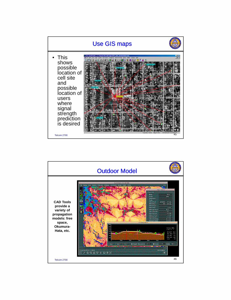
Use GIS mapsUse GIS maps

• This shows possible location of cell site and possible location of users where

Telcom 2700 45

where signal strength prediction is desired

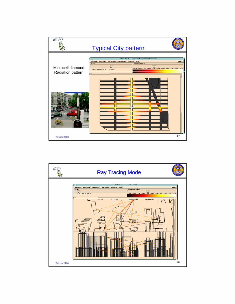
Outdoor ModelOutdoor Model

CAD Tools provide a variety of

propagation models: free

space, Okumura-

Telcom 2700 46

Hata, etc.

Typical City pattern

Microcell diamondR di ti ttRadiation pattern

Telcom 2700 47

Ray Tracing ModeRay Tracing Mode

Telcom 2700 48

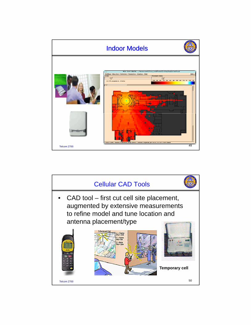
Indoor ModelsIndoor Models

Telcom 2700 49

Cellular CAD Tools

• CAD tool – first cut cell site placement, augmented by extensive measurements t fi d l d t l ti dto refine model and tune location and antenna placement/type

Telcom 2700 50

Temporary cell

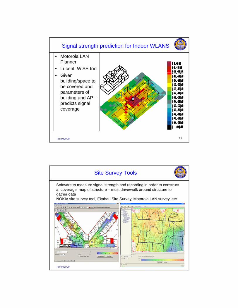
Signal strength prediction for Indoor WLANS

• Motorola LAN Planner

• Lucent: WiSE tool

• Given building/space to be covered and parameters of building and AP –predicts signal

Telcom 2700 51

coverage

Site Survey Tools

Software to measure signal strength and recording in order to construct a coverage map of structure – must drive/walk around structure to gather dataNOKIA site survey tool, Ekahau Site Survey, Motorola LAN survey, etc. y , y, y,

Telcom 2700 52

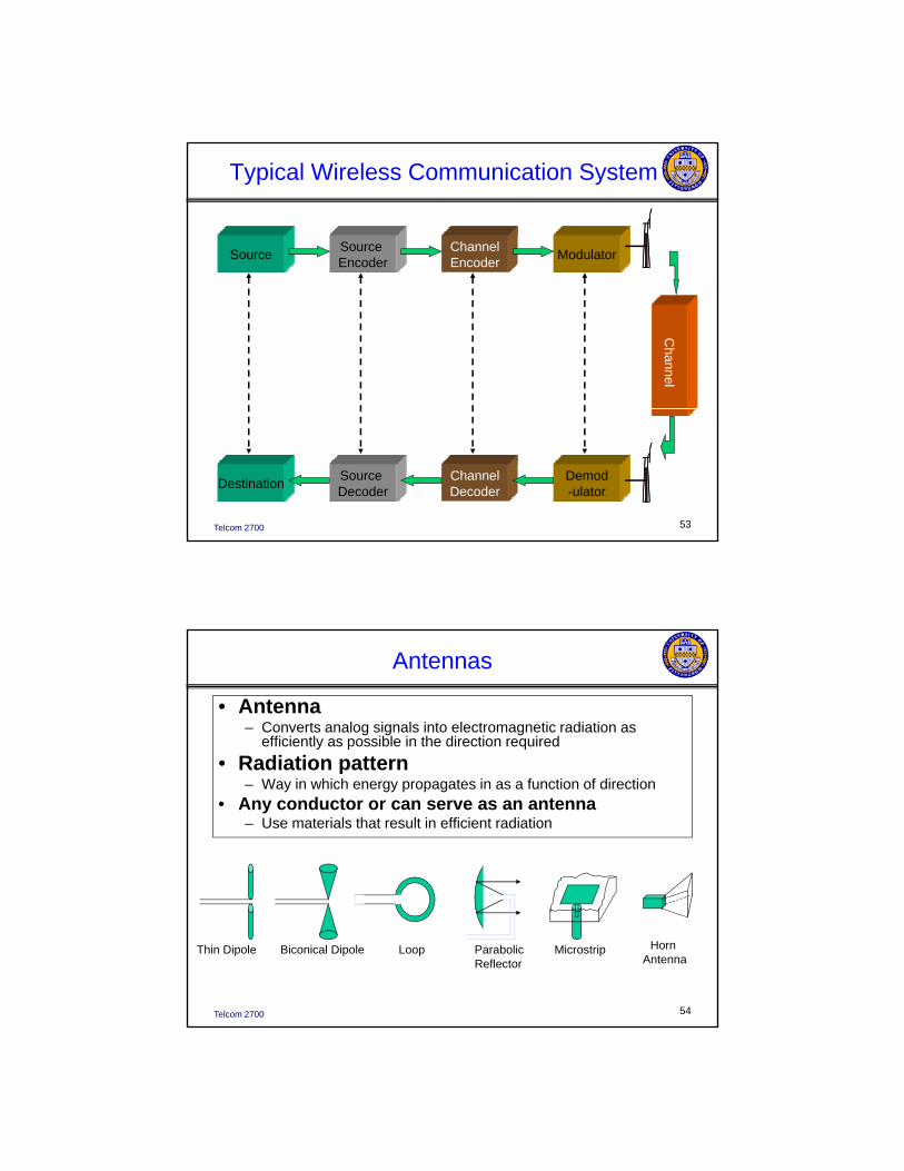
Typical Wireless Communication System

SourceSource Encoder

ChannelEncoder

Modulator

Channel

Telcom 2700 53

DestinationSource Decoder

ChannelDecoder

Demod-ulator

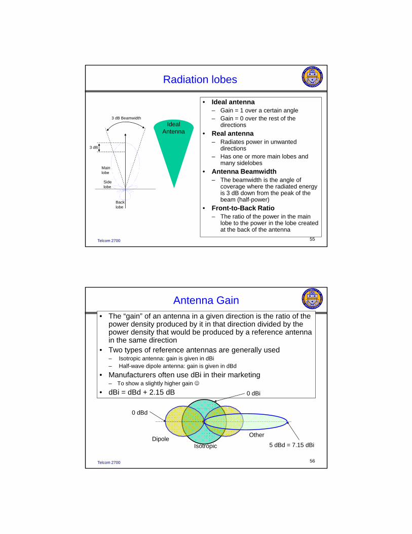
Antennas

• Antenna – Converts analog signals into electromagnetic radiation as

efficiently as possible in the direction required

• Radiation pattern• Radiation pattern– Way in which energy propagates in as a function of direction

• Any conductor or can serve as an antenna– Use materials that result in efficient radiation

Telcom 2700 54

Thin Dipole Biconical Dipole Loop Parabolic Reflector

Microstrip Horn Antenna

Radiation lobes

• Ideal antenna– Gain = 1 over a certain angle– Gain = 0 over the rest of the

directions3 dB Beamwidth

Ideal directions

• Real antenna– Radiates power in unwanted

directions– Has one or more main lobes and

many sidelobes

• Antenna Beamwidth– The beamwidth is the angle of

coverage where the radiated energy

Mainlobe

Sidelobe

3 dB

IdealAntenna

Telcom 2700 55

coverage where the radiated energy is 3 dB down from the peak of the beam (half-power)

• Front-to-Back Ratio– The ratio of the power in the main

lobe to the power in the lobe created at the back of the antenna

lobe

Backlobe

Antenna Gain• The “gain” of an antenna in a given direction is the ratio of the

power density produced by it in that direction divided by the power density that would be produced by a reference antenna in the same directionT t f f t ll d• Two types of reference antennas are generally used– Isotropic antenna: gain is given in dBi– Half-wave dipole antenna: gain is given in dBd

• Manufacturers often use dBi in their marketing– To show a slightly higher gain

• dBi = dBd + 2.15 dB 0 dBi

Telcom 2700 56

0 dBd

5 dBd = 7.15 dBiIsotropicDipole

Other

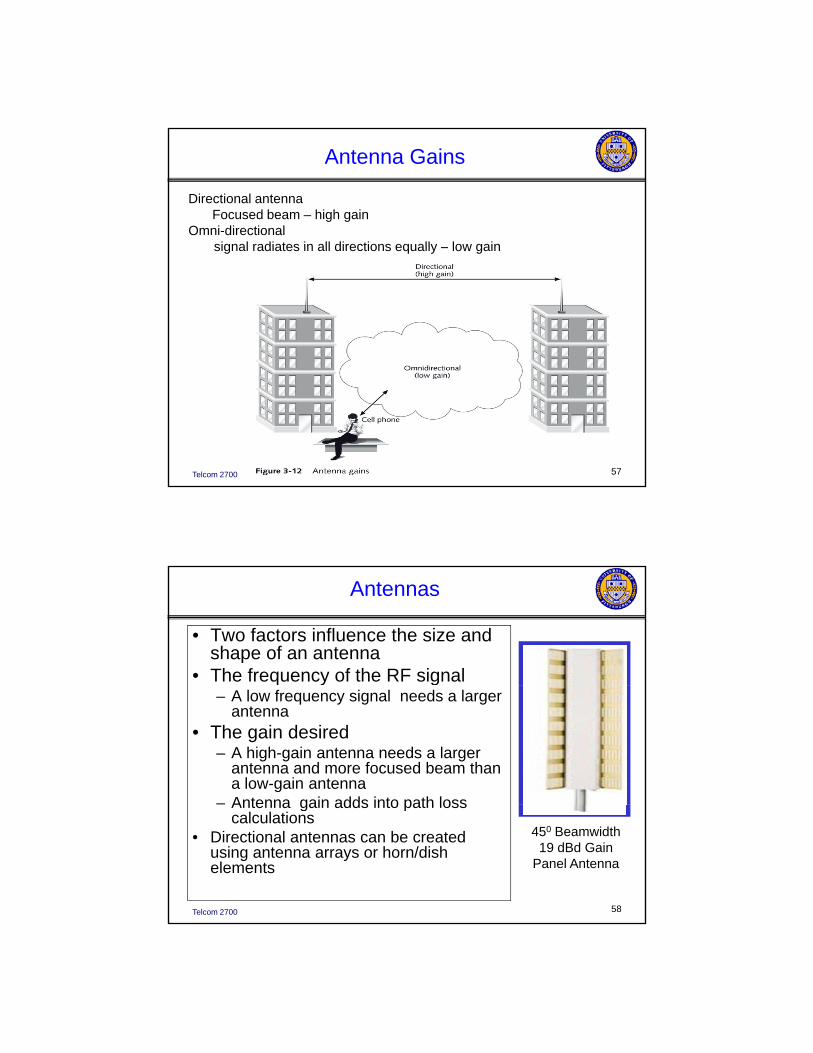
Antenna Gains

Directional antennaFocused beam – high gain

Omni-directional signal radiates in all directions equally – low gainsignal radiates in all directions equally – low gain

Telcom 2700 57

Antennas

• Two factors influence the size and shape of an antenna

• The frequency of the RF signalq y g– A low frequency signal needs a larger

antenna • The gain desired

– A high-gain antenna needs a larger antenna and more focused beam than a low-gain antenna

– Antenna gain adds into path loss

Telcom 2700 58

Antenna gain adds into path loss calculations

• Directional antennas can be created using antenna arrays or horn/dish elements

450 Beamwidth19 dBd Gain

Panel Antenna

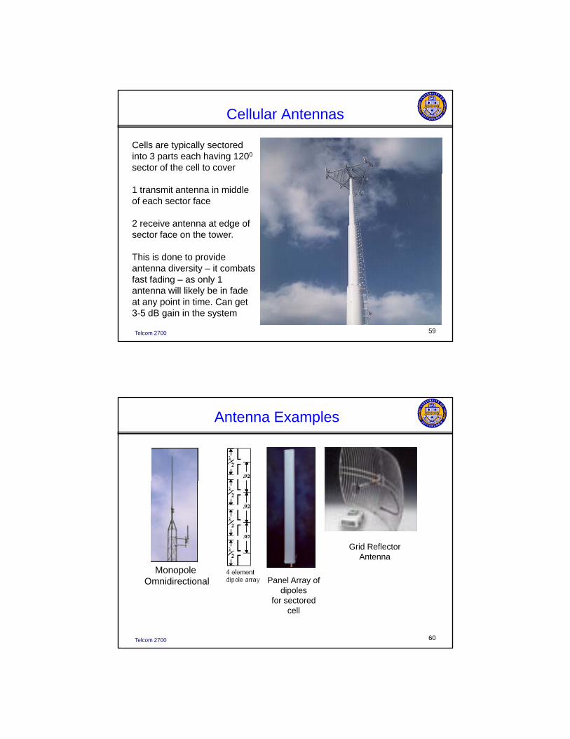
Cellular Antennas

Cells are typically sectored into 3 parts each having 1200

sector of the cell to cover

1 transmit antenna in middle of each sector face

2 receive antenna at edge of sector face on the tower.

This is done to provide

Telcom 2700 59

This is done to provide antenna diversity – it combats fast fading – as only 1 antenna will likely be in fade at any point in time. Can get 3-5 dB gain in the system

Antenna Examples

Grid ReflectorAntenna

Telcom 2700 60

Monopole Omnidirectional Panel Array of

dipoles for sectored

cell

Link Budget

• Used to plan useful radio coverage of link/cells– Relates transmit power, path losses, margins,

interference, etc.interference, etc.

– Used to find max allowable path loss on each link

– Typical Factors in Link Budget• Transmit Power,

• Antenna Gain, Diversity Gain,

• Receiver Sensitivity

Telcom 2700 61

• Shadow Margin, Interference Margin,

• Vehicle Penetration Loss, Body Loss, Building Penetration, etc.. (Typical values from measurements used)

– Gains are added, Losses are subtracted – must balance

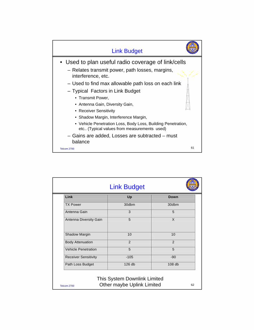
Link BudgetLink Up Down

TX Power 30dbm 30dbm

Antenna Gain 3 5

Antenna Diversity Gain 5 X

Shadow Margin 10 10

Body Attenuation 2 2

Vehicle Penetration 5 5

Telcom 2700 62

Receiver Sensitivity -105 -90

Path Loss Budget 126 db 108 db

This System Downlink LimitedOther maybe Uplink Limited