wireless backhaul (and access) at millimeter wave frequencies
TRANSCRIPT

Wireless Backhaul (and Access) at Millimeter Wave Frequencies!
!!!!!
David J. Love!Associate Professor!
School of Electrical and Computer Engineering!Purdue University!
Portions of research supported in part by Nokia Siemens Networks!

2
Need for Small Cells
n Many dire predictions for throughput demand
n Solution higher frequency reuse (Cooper’s law)!
n Move users physically closer to an assumed high rate link!
n Backhaul arguably the key challenge! n Will backhaul end up being the bottleneck?!

3
Backhaul in the News!n 2009 - AT&T iPhone troubles:!
!
n Touted backhaul upgrades (e.g., Verizon fiber and wireless, AT&T enhanced backhaul) !
n 2011 - Alternative backhaul industry against failed AT&T-T-Mobile deal!
n 2012 - Study saying backhaul demand scales 10x by 2016!
“The executive says some Apple staffers fumed last year when AT&T told them of its plans to hype cell tower upgrades without investing in backhaul capacity” – Businessweek, Aug. 23, 2009 (http://www.businessweek.com/technology/content/aug2009/tc20090823_412749.htm)

4
Flavors of Backhaul
n Wired backhaul still very common (60%-70% copper in US, 40% wired globally) !
n Wireless backhaul growing!n Must avoid “usable
spectrum” ( < 3GHz)!n Future backhaul possibilities!
n Copper/Fiber!n In-band backhaul!n 5-38GHz wireless!n mmWave wireless!n 100-400 GHz wireless!n Free space optics!
!
Source: Fibertower SEC filing!

5
Possible Architecture!
n Networks of small cells (pico) connected by millimeter wave backhaul (~50 meter links) !
n User could access with 4G+ or mmwave radios!n Likely Requirements!
n 1) Must be easy to install!n 2) At least one node per network sees macro (beamforming) or
can collaborate (distributed beamforming [Madhow])!n 3) Has a backup! (e.g., in-band backhaul)!n 4) Nodes could use self-organizing topology [Singh et al]!

6
Two Challenges !
n Challenge 1) Aligning the beam!n Narrow beam = Hard to align!!n Limited resources for alignment!
n Challenge 2) Deployment and ! mounting!
n Pole mounting!n Wind!

7
Challenge 1: Sounding and Beam Alignment!
n Beamforming at Tx and Rx is critical!!
!
n Receiver does not have access to each element output!! Observes noisy not!
n Must sound channel using training sequence to figure out where beams must point!
!!!!!
y[k] = z⇤Hfs[k] + n[k]
z⇤Hf Hf
kzk = kfk = 1

8
Initial Beam Alignment!
n Figure out how to point beam with little initial side info!n New user, new installation, blockage, etc!n Assume training sequence!
n Must solve! using observations! !n Interesting prior work for indoor millimeter wave (e.g.,
[Wang et al, Tsang et al])!n Alignment time may be highly constrained in some situations
(i.e., L small)!n Can take noisy subspace samples (possibly adaptively) with ! and usually !
max g(z, f) = |z⇤Hf |2z⇤[`]Hf [`] + n[`], ` = 1, 2, . . . , L
LL ⌧ MrMt L = O(Mr +Mt)

9
Understanding Beam Alignment!
n Possibly many antennas!
n Very few dominant paths (usually rank one)!
n Often!!n Focus on case when finite beam directions used!
H 2 CMr⇥Mt
rank (H)
min(Mr,Mt)⇡ 0
z 2 Ar = {z1, . . . , zNr}, f 2 At = {f1, . . . , fNt}

10
Problems to Solve!
1) Alignment Given Observations! Given sounding pairs and samples ! how do we choose to maximize SNR?!!2) Sounding Problem! How do we select sounding beamformer/combiner ! pair ? !
n Random (non-adaptive) sounding!n Adaptive sounding!
(z, f)
(z[`], f [`])
{y[`]}L`=1{(z[`], f [`]}L`=1

11
Topic 1: Beam Alignment – Hard Decision!
n Beam alignment typically works by probing the channel with possible pairs !
n Hard alignment: Best alignment chosen simply as max receive power pair!
n Has a particularly appealing interpretation with array manifold!
(z, f) = argmax
(z[`],f [`])|z⇤[`]Hf [`] + n[`]|2
{(z, f), z 2 Ar, f 2 At}

12
Beam Alignment is Related to….!
n Problem actually one of rank one approximation!
n Must approximate using i) very few subspace samples and ii) low rank assumption!
!n Much work in this area (e.g., [Candes, Tao],[Candes,Plan],
[Keshavan,Montanari,Oh])!
Matrix completion idea: Randomly sample entries of a very large dimension rank r matrix. Find rank at most r matrix to minimize some distortion relative to this data!
Matrix Completion!
argmax
z,f|z⇤Hf |2 = argmin
z,fmin
�kH� �zf⇤kF

13
Example of Matrix Completion!
n Samples drawn uniformly!n Often important to “spread” samples out!n Use algorithm that creates low rank approximation (e.g., OPTSPACE)!
!
2
6666664
h1,1 h1,2 h1,3 h1,4 h1,5 h1,6
h2,1 h2,2 h2,3 h2,4 h2,5 h2,6
h3,1 h3,2 h3,3 h3,4 h3,5 h3,6
h4,1 h4,2 h4,3 h4,4 h4,5 h4,6
h5,1 h5,2 h5,3 h5,4 h5,5 h5,6
h6,1 h6,2 h6,3 h6,4 h6,5 h6,6
3
7777775
Observed!values!

14
Beam Alignment + Matrix Completion?!
n Possibly have subspace side info of channel!n Array manifold!
n Reconstruction limited to!n Can be viewed as direction matrix completion!
n Soft alignment: Minimize subspace distance from observed points!
A(✓)
z 2 Ar, f 2 At
G =
2
64z⇤1...
z⇤Nr
3
75H [f1 · · · fNt ]Find largest !entry of !G
argminz,f
min�
LX
`=1
|y[`]� �z⇤[`]zf⇤f [`]|2
= argmax
z,f
���PL
`=1 y⇤[`]z⇤[`]zf⇤f [`]
���2
|z⇤[1]zf⇤f [1]|2 + · · ·+ |z⇤[L]zf⇤f [L]|2

15
Topic 2) Adaptive Sounding!
n Reciprocity or feedback allows adaptive sounding!!
n Can choose pair prior to sounding!
n Questions:!!How can Tx help Rx align?!!How can Rx help Tx align?!!What role does noise play?!
!
z⇤[`]Hf [`] + n[`], ` = 1, 2, . . . , L(z[`], f [`])

16
Adaptive Sounding Approach!
n Suppose channel rank one and!
n If Tx uses a near optimal beamformer, large!
n If Rx uses a near optimal combiner, large !!
n Ping-pong alignment!!- Tx sounds its best known direction, Rx aligns!!- Tx sounds various directions, Rx points in best known ! direction!
H = h1h⇤2
|h⇤2f [`]|
|z⇤[`]h1|Higher SNR Rx observations!
Higher SNR Tx observations!

17
Hard Decision Alignment!
n Works very well with LOS array manifold concepts!
n Use progressively narrower beams!n Motivates sub-codebooks!
Wider beam
Narrower beam
W1
W2
W3
NB
N2B
N3B
n Important points:!1) Each path in tree is a !direction for further search!2) Different path sub-codebooks must “overlap”!n Continue to probe area
of strongest return!

18
Soft Decision Alignment – Understanding Matrix Completion Limitations!
n Matrix completion obviously difficult for many matrices!
Incoherence measure [Candes]: Let SVD be we require as small as possible with!!n Intuitively, want singular vectors to be equal gain because we
sample with vectors of form !
2
664
0 0 0 00 0 0 00 0 1 00 0 0 0
3
775Reconstructs to !all zero matrix!!
H =X
kr
�kukv⇤k
kukk1 p
µ/Mr kvkk1 p
µ/Mt
µ
[0 · · · 0 1 0 · · · 0]T

19
Understanding Incoherence!
n Matrix completion assumes “peaky” subspace sampling!
n Incoherence stipulates that singular vecs are not too distant from vectors in !
n Channel Sounding: Singular vectors in array manifold!
n By-product: Would allow access in crowded user scenarios! (but is it legal????)!
Apeaky
Apeaky = {e1, . . . , eM}columns of identity matrix!
Omnidirectional Sounding!!

20
Alignment Comparison w/ SNR !n LOS 32x32 !n ULA!n AoD and AoA
uniform in [-60°,60°]!
n Adaptive soft alignment gives ~1dB improvement!
n Random alignment comes at >5db penalty!!
Sounding SNR (db)!
Beam
form
ing
Gai
n (d
b)! 4096 samples!
48 samples!

21
Comparison with WiGig Alignment!n Beamforming Gain!
21
−20 −15 −10 −5 0 5 10 155
10
15
20
25
30
Bea
mfo
rmin
g G
ain,
GBF
(dB
)
SNR (dB)
Exhaustive searchExt. Multi−level searchSTD 802.11ad : one−sided search
-‐ TX, RX use ULA mul/-‐level codebook with -‐ (three level) -‐ (branch expansion) -‐ (extended search branches) -‐ Carrier frequency : 60 GHz -‐ Bandwidth : 400 MHz -‐ Rician fading channel with K-‐factor = 13 dB -‐ Modeled with 4 mul/paths
-‐
K = 3NB = 4
(MT = MR = 32)
Nk = 8
22
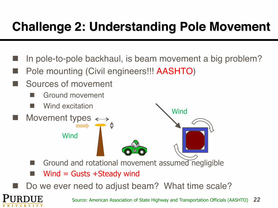
Challenge 2: Understanding Pole Movement!
n In pole-to-pole backhaul, is beam movement a big problem? !n Pole mounting (Civil engineers!!! AASHTO)!n Sources of movement!
n Ground movement!n Wind excitation!
n Movement types!
n Ground and rotational movement assumed negligible n Wind = Gusts +Steady wind!
n Do we ever need to adjust beam? What time scale?!
Wind
Source: American Association of State Highway and Transportation Officials (AASHTO)
Wind

23
Lamp Post
(vertical view)
Low pressure zone
Constant pole sway
Wind
movement
movement
Wind
Wind Induced Movment!
n Cause 1: Mean and Gust-based movement!n Cause 2: Flow of wind over lamppost!
§ Vortex shedding!
§ Low pressure zones cause movement perpendicular to wind direction
§ Cause constant vibration !
wind! Vortex shedding!gusting!

24
Models of Movement!
n Wind assumed well modeled by a stationary Gaussian process + velocity dependent mean [Davenport]!
n Davenport filter shapes spectrum (low-pass)!n Aero admittance maps velocity perturbation to force
(Recall: Drag force proportional to squared velocity)!
n Mechanical transfer gives response to force!
Davenport !Filter!
Aero !Admittance!
Mechanical !Transfer!
g(t) `(t)
velocity! force! movement!w(t)
wwhite(t)
Structural damping ratio Natural frequency
(W + w(t))2 ⇡ W2+ 2Ww(t)
|Hm(!)|2 =1
(!2n � !2) + (2⇣!n!)2

25
Beam Outage!
n Outage Probability
0 10 20 30 40 50 60 700
0.1
0.2
0.3
0.4
0.5
0.6
0.7
0.8
0.9
1
mean wind speed, v (m/s)
Perc
enta
ge o
f tim
e in
out
age,
Pou
t
Wind−induced beam outage, moderate turbulence (0.1 intensity)
M = 128M = 256M = 384M = 512

26
Role of Tolerable SNR Loss!
n Received beam gain faded under n Antenna Array -‐ ULA at transmiUer / receiver n Mean wind-‐velocity : (extreme gust)
SNRloss
M = 256
0 5 10 15 20 25 30−0.4
−0.3
−0.2
−0.1
0
0.1
0.2
0.3
0.4
Time (sec)
Bea
m−o
utag
e A
ngle
(deg
)
Beam−outage Analysis
SNRloss = 1SNRloss = 3SNRloss = 5SNRloss = 7SNRloss = 9
v = 30 [m/s]
27
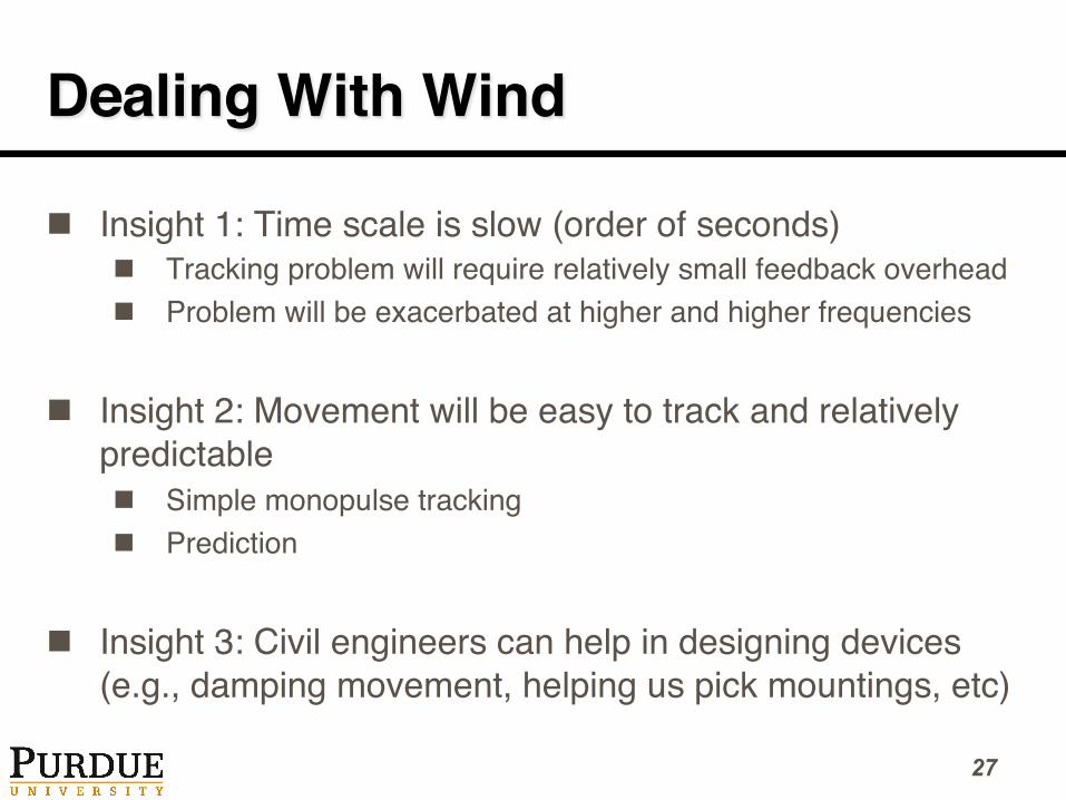
Dealing With Wind!
n Insight 1: Time scale is slow (order of seconds)!n Tracking problem will require relatively small feedback overhead!n Problem will be exacerbated at higher and higher frequencies!
n Insight 2: Movement will be easy to track and relatively predictable!n Simple monopulse tracking!n Prediction!
n Insight 3: Civil engineers can help in designing devices (e.g., damping movement, helping us pick mountings, etc)!

28
mmWave Beamforming Summary
§ Economic and technical issues motivate smaller cells
§ Backhaul challenges are tremendous
§ There is no magic bullet for backhaul!
§ Beam alignment critical
§ Environmental factors influence beam alignment