No. 13-4

Window Shopping

Oz Shy

Abstract: The terms “window shopping” and “showrooming” refer to the activity in which potential buyers visit a brick-and-mortar store to examine a product but end up either not buying it or buying the product from an online retailer. This paper analyzes potential buyers who differ in their preference for after-sale service that is not offered by online retailers. For some buyers, making a trip to the brick-and-mortar store is costly; however, going to the store to examine the product has the advantage of mitigating the uncertainty as to whether the product will suit the buyer’s needs. The model shows that the number of buyers engaged in window shopping behavior exceeds the optimal number, both under duopoly and under joint ownership of the online and walk-in store outlets. Keywords: window shopping, showrooming, brick-and-mortar stores, online shopping, online retailers, virtual stores, bricks and clicks

JEL Classifications: L1, L8, G21 Oz Shy is an economist in the research department of the Federal Reserve Bank of Boston. His e-mail address is oz.shy@bos.frb.org. This paper, which may be revised, is available on the web site of the Federal Reserve Bank of Boston at http://www.bostonfed.org/economic/wp/index.htm. I thank Suzanne Lorant, Elizabeth Murry, Scott Schuh, and Bob Triest for most valuable comments on an earlier draft. The views expressed in this paper are those of the author and do not necessarily represent the views of the Federal Reserve Bank of Boston or the Federal Reserve System.

This version: May 6, 2013

1 Introduction

The magazine Consumer Reports recently surveyed over 10,000 readers and found that 18 percent

of them bought electronic products online after they had examined the products in a brick-and-

mortar store. More than half of this group eventually bought from Amazon.com.1 The practice

of inspecting products at a walk-in retailer before buying them online will be referred to in this

paper as window shopping, or showrooming.2

Online shopping in the United States accounted for 7 percent of all retail sales in 2011 and

2012. However, according to a Forrester Research Inc. report “U.S. Online Retail Forecast, 2011 to

2016,” U.S. e-retail will represent 9 percent of all consumer purchases by 2016.3 Therefore, online

shoppers in the United States will spend $327 billion in 2016, up 45 percent from $226 billion in

2012 and up 62 percent from $202 billion in 2011. These figures represent a compound annual

growth rate of 10.1 percent over the five-year forecast period.

This paper constructs a model of potential buyers who differ in their preference for after-sale

services that are not offered by online sellers. Technically speaking, the walk-in retailer and the

online seller are assumed to be vertically differentiated, which implies that, in the absence of the

transportation costs incurred from going to the store, all buyers would prefer buying at the brick-

and-mortar store if its price did not exceed the online price.

While making a trip to the store is costly for some buyers, it has the informational advantage

of mitigating the uncertainty as to whether the product will suit the buyer’s needs. The paper

derives equilibrium prices, profits, consumer welfare, and social welfare in order to examine the

relationship between the equilibrium number of window shoppers and the socially optimal num-

ber. The analysis first concentrates on a duopoly market structure where an online seller and a

walk-in retailer compete to attract potential buyers. The same investigation is then conducted for

single ownership of (or a merger between) the online and the brick-and-mortar outlets.

1See, “Get the best deal,” Consumer Reports, December 2012, p. 24.2Window shoppers also includes recreational shoppers (not analyzed in this paper) who simply spend time in shop-

ping malls browsing and visiting stores. The attitudes of this type of consumers are described in Jarboe and McDaniel(1987) and Cox, Cox, and Anderson (2005).

3See, http://webprod.forrester.com/US+Online+Retail+Forecast+2011+To+2016/fulltext/-/E-RES60672?objectid=RES60672.

1

The main conclusion from the analysis in this paper is that given equal marginal costs of the

sellers, the equilibrium number of browsers at the walk-in store exceeds the optimal number.

This is because once a potential buyer travels to the store, transportation costs should be viewed

as sunk and therefore should not influence a buyer’s decision where to purchase the product.

Hence, if this potential buyer finds the product to be suitable for his or her needs, this buyer

should buy it at the store rather than online because the store provides after-sale service and the

online seller does not. This distortion is created because the online seller sells the product at a

price below the store’s price in order to attract some buyers to purchase the product online after

they have inspected it at the walk-in store and found it suitable. The magnitude of this distortion

is diminished (or eliminated) if the store’s marginal cost increases relative to the online seller’s

marginal cost.

The analysis in this paper applies to products that potential buyers can benefit from inspecting

prior to purchase. It is assumed that after physically inspecting the product and discussing the

pros and cons with a live salesperson who demonstrates the product, the potential buyer can de-

cide whether the product is suitable for his needs. Appliances are good examples of such products.

Therefore, the main economic tradeoff modeled here is the consumer’s tradeoff between incurring

the transportation costs associated with traveling to a brick-and-mortar store to inspect the prod-

uct and forgoing the benefits derived from mitigating uncertainty as to whether the product suits

the buyers’ needs.

The model developed in this paper draws heavily on Shin (2007). Both papers model con-

sumers who are uncertain as to whether the product suits their needs and therefore would benefit

from expert, in-store advice on this matter. In addition, in both models, a retailer that does not

provide pre-sale service may be able to free ride on a pre-sale service provided by the rival ven-

dor. However, a closer look at both models reveals some substantial differences. (a) In Shin’s

model, the two retailers are identical in all respects (including buyers’ transportation costs) and

both are capable of providing identical pre-sale services. In the present model, the online and the

walk-in sellers differ in their ability to provide pre- and post-sale services. In addition, buyers’

transportation and shopping time costs depend on whether they shop online or at the walk-in

2

store. Consequently, (b) in Shin’s model, if the two retailers charge identical prices, all potential

buyers (informed and uninformed) would patronize the retailer that offers the pre-sale service. In

contrast, in this model, under equal prices each seller will face some positive demand.

These differences imply that Shin’s model is better suited to study competition between full-

service and discount brick-and-mortar stores than to study online versus walk-in retailers. In

contrast, the present model is better suited to study competition between independent online

sellers and brick-and-mortar sellers, which are differentiated not only by their pre-sale service but

also by their post-sale service, than to study competition between full-service and discount sellers.

This is because the first-best allocation in Shin’s model can be supported by a single retailer (if the

price is maintained at the competitive level), whereas in the present model a first-best allocation

may be supported by coexistence between the online and the walk-in stores. This may be the

reason why Shin’s paper does not include a welfare analysis.

Pre-sale service provision arises in Shin’s model as a strategy of one retailer to differentiate

itself from another retailer, in order to avoid intense price competition that would otherwise elim-

inate all profits. This theory shows that one retailer always benefits from bundling service with

the sale of a product. (See Carbajo, De Meza, and Seidmann (1990), Horn and Shy (1996), and

their references). In the absence of bundling, buyers view the products (brands) as homogeneous

and choose the retailer with the lowest price. In that circumstance, price competition affecting all

consumers reduces prices to marginal cost. This literature argues that a store offers more services

than its competitors only for the sake of segmenting the buyers’ market into two groups according

to buyers’ benefits from consuming these services. Market segmentation is needed to soften price

competition.

Friberg, Ganslandt, and Sandstrom (2001) develop an analytical model of price competition

between an online and a physical store in the absence of window shopping. On the empirical

side, Farag, Krizek, and Dijst (2006), Farag et al. (2007), Forman, Ghose, and Goldfarb (2009),

Cao (2012), and Cao, Xu, and Douma (2012) investigate the effect of online shopping and online

search on traditional shopping. Brynjolfsson and Smith (2000) find that online prices are 9 to 16

percent lower than prices in conventional retail outlets, depending on whether taxes, shipping,

3

and shopping costs are included in the final price.

This study is organized as follows: Section 2 constructs a model. Section 3 solves for the equi-

librium prices and market shares under duopoly. Section 4 conducts a welfare analysis. Section 5

analyzes joint ownership of the online and walk-in store outlets. Section 6 analyzes the conse-

quences of unequal marginal costs. Section 7 concludes.

2 The Model

The market consists of two sellers: an online seller (denoted by O) and a walk-in retailer that sells

only at a specific location (the store in what follows, and denoted by S). Both the online and

the walk-in retailer sell the same product but may charge different prices denoted by pO and pS ,

respectively. All potential buyers are fully informed of these prices before they make any purchase

decision.

The brick-and-mortar store offers an after-sale service that the online seller does not provide.

After-sale service may include: (a) easy return for any reason or a replacement of a defective

product, (b) help in the activation of related services and the installation of compatible software,

and (c) assistance in learning how to operate the product.

2.1 Potential Buyers

There are 2N potential buyers who are uniformly distributed on the interval [0, 1] according to

increased preference for after-sale service, denoted by s ∈ [0, 1] (“s” stands for “service” benefits).

Therefore, buyers indexed by s close to 1 derive a great deal of benefit from after-sale service,

whereas buyers indexed by s = 0 do not benefit at all from after-sale service. Figure 1 illustrates

how potential buyers are distributed according to the value they place on the potential benefits of

after-sale service.

The term potential buyers should be distinguished from buyers because not all individuals will

find that the product suits their needs. In this case, we will say the product is unsuitable. Each

buyer estimates that the product will fulfill her or his needs with probability σ (the Greek letter

4

“sigma” stands for “suitable” here), and hence will be unsuitable with probability 1 − σ, where

0 < σ < 1.

One advantage of going to a walk-in store rather than buying directly online is that the store

allows potential buyers to examine the product and decide whether it suits their needs before

making a purchase. However, traveling to the store is costly. Let t ∈ {0, τ} denote the transporta-

tion cost of traveling to the store. It is assumed that N potential buyers bear a cost of t = τ > 0

associated with traveling to the store. The other N potential buyers do not bear any cost (t = 0).

-s (service benefits)

0 1

6

2σN

2N

Expected number of buyers (for whom the product is suitable)

Expected no. of individuals for whom the product is not suitable

# buyers per type

Figure 1: Heterogeneous Potential Buyers

Let v (v > 0) denote the basic value derived from consuming a suitable product. The utility

of a buyer indexed by s ∈ [0, 1] with transportation costs t ∈ {0, τ} is assumed to take the form

u(s, t) =σv − pO Buys directly online (without first going to the store)

−t Travels to the store and finds the product unsuitable

v − pO − t Travels to the store and finds the product suitable, but buys online

v − pS + s− t Travels to the store, finds the product suitable, and buys at the store.

(1)

Figure 2 illustrates the dynamic decision tree facing each potential buyer.

Choosing to buy the product online without first going to the store saves the transportation

cost t. However, by forgoing the trip the buyer is unable to inspect the product to determine

whether it suits his needs before making the purchase. Thus, the expected gain to a buyer who

shops online without first going to the store is σv + (1 − σ)0 − pO, which corresponds to the left

branch in Figure 2 and the first row in equation (1).

5

BuyerBuys online

uuuuuuuuuuuTravels to the store

IIIIIIIIIII

σv − pO NatureProduct suitable (σ)

uuuuuuuuuuuProduct unsuitable (1− σ)

IIIIIIIIIII

BuyerBuys online

uuuuuuuuuuuBuys at store

IIIIIIIIIII −t

v − pO − t v − pS + s− t

Figure 2: Buyer’s Decisions and Outcomes

The terminal nodes stemming from the right-hand-side branches in Figure 2 show that trav-

eling to the store generates transportation costs t ∈ {0, τ} regardless of whether the product is

eventually found to be suitable or unsuitable. If the product is deemed suitable, the buyer can

then choose between purchasing it at the store or leaving the store and buying it online. If the

product is unsuitable, no purchase is made and the buyer leaves the store with a loss of t.

To summarize, traveling to the store removes the uncertainty as to whether the product is use-

ful to the buyer. Buying online without first going to the store saves the transportation cost t, but

leaves the buyer with the risk that the purchased product may not prove appropriate. Therefore,

the expected value of buying online without seeing the product at the store is reduced from v to

σv. In addition, all online buyers (whether or not they visit the walk-in store) fail to receive the

after-sale service benefit, s.

The following assumption ensures that, in equilibrium, each type of seller attracts some buy-

ers.4

ASSUMPTION 1. The transportation cost parameter is bounded from above and below. Formally,

σ(1− σ2)3σ2 + σ + 2

def= τmin < τ < τmax def

=σ(3σ2 + 5)

5σ2 + 3.

Reversing the inequality on the right-hand-side in Assumption 1 would make a visit to the store

4It can be shown that the interval defined in Assumption 1 is nonempty, because τmax > τmin for every σ > 0.

6

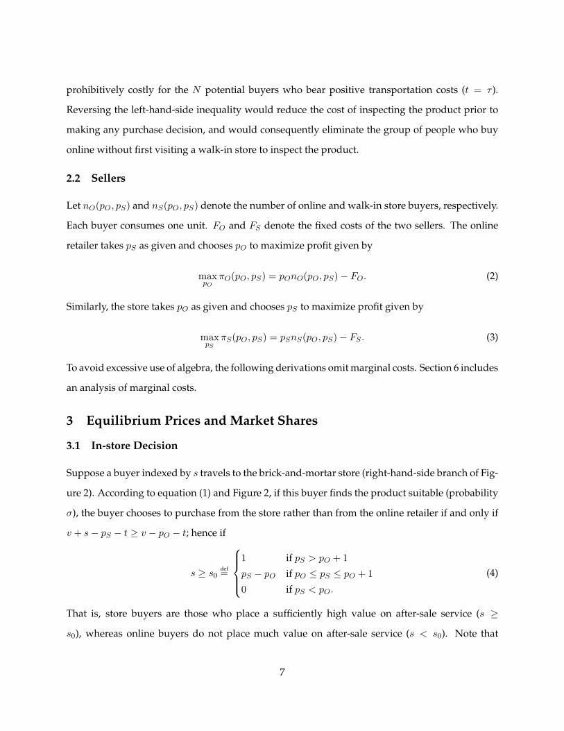
prohibitively costly for the N potential buyers who bear positive transportation costs (t = τ ).

Reversing the left-hand-side inequality would reduce the cost of inspecting the product prior to

making any purchase decision, and would consequently eliminate the group of people who buy

online without first visiting a walk-in store to inspect the product.

2.2 Sellers

Let nO(pO, pS) and nS(pO, pS) denote the number of online and walk-in store buyers, respectively.

Each buyer consumes one unit. FO and FS denote the fixed costs of the two sellers. The online

retailer takes pS as given and chooses pO to maximize profit given by

maxpO

πO(pO, pS) = pOnO(pO, pS)− FO. (2)

Similarly, the store takes pO as given and chooses pS to maximize profit given by

maxpS

πS(pO, pS) = pSnS(pO, pS)− FS . (3)

To avoid excessive use of algebra, the following derivations omit marginal costs. Section 6 includes

an analysis of marginal costs.

3 Equilibrium Prices and Market Shares

3.1 In-store Decision

Suppose a buyer indexed by s travels to the brick-and-mortar store (right-hand-side branch of Fig-

ure 2). According to equation (1) and Figure 2, if this buyer finds the product suitable (probability

σ), the buyer chooses to purchase from the store rather than from the online retailer if and only if

v + s− pS − t ≥ v − pO − t; hence if

s ≥ s0def=

1 if pS > pO + 1

pS − pO if pO ≤ pS ≤ pO + 1

0 if pS < pO.

(4)

That is, store buyers are those who place a sufficiently high value on after-sale service (s ≥

s0), whereas online buyers do not place much value on after-sale service (s < s0). Note that

7

transportation costs are treated as sunk after the potential buyer travels to the store, and therefore

do not factor into a buyer’s purchase decision after a store visit is made. For this reason t does not

appear in (4).

3.2 The Decision to Visit the Store

All N potential buyers who do not incur transportation costs (t = 0) travel to the store to inspect

the product. In this group, those who find the product suitable decide whether to buy the product

at the store or to buy it online. This decision depends on the benefits buyers derive from after-

sale services, as given in equation (4). The market division of buyers with no transportation costs

between the two retailers is depicted in the top part of Figure 3.

-s (service benefits)

0 1

-s (service benefits)

0 1

(t = τ )

(t = 0)

sτ

Travel and buy

at the store if suitableBuys directly online

s0

Window Shoppers: Visit the store

Then, buy online if suitable

Travel and buy at

the store if suitable

Figure 3: Division of Market Shares between Walk-in and Online Retailers. Top: Shoppers with NoTransportation Costs (t = 0). Bottom: Shoppers with Transportation Costs (t = τ ).

In contrast to potential buyers who do not incur transportation costs, some of the N potential

buyers who do incur transportation costs τ will not find it beneficial to travel to the walk-in store

to inspect the product. In particular, buyers who do not place significant value on after-sale service

may decide to purchase the product online without first inspecting it at the store.

The right-hand-side branches of the decision tree depicted in Figure 2 imply that the expected

utility from visiting the walk-in store of a service-oriented buyer (s ≥ s0) with high transportation

costs (t = τ ) is

(1− σ)(−τ) + σ(v + s− pS − τ), for buyers s ≥ s0. (5)

The first term in equation (5) is the expected loss from finding the product unsuitable after traveling

8

to the store to examine the product. The second term is the expected gain from buying a suitable

product at the walk-in store.

Moving to the beginning of the tree displayed in Figure 2, a service-oriented buyer (s ≥ s0)

with high transportation costs (t = τ ) will choose to travel to the store rather than buy online

without going to the store if and only if

(1− σ)(−τ) + σ(v + s− pS − τ) ≥ σv − pO, or

s ≥ sτ def=

1 if σpS > pO − τ + σ

pS + τ−pOσ if pO − τ ≤ σpS ≤ pO − τ + σ

0 if σpS < pO − τ.(6)

The market division among buyers with high transportation cost is depicted on the bottom part

of Figure 3.

Similarly, a buyer with high transportation costs (t = τ ) who does not place much value on

after-sale service (s < s0) will choose to buy online without first inspecting the product at the

walk-in store (over visiting the store and then buying the product online if it is deemed suitable)

if and only if

σv − pO ≥ (1− σ)(−τ) + σ(v − pO − τ), or (1− σ)pO < τ. (7)

The condition listed in equation (7) indicates that the online price has to be sufficiently low relative

to the transportation cost to deter less-service-oriented potential buyers from visiting the store

before buying online. This condition will have be verified after we solve for the equilibrium online

price, pO. Also note that equations (4) and (6) imply that sτ > s0 if condition (7) is satisfied. Hence,

buyers who incur transportation costs and are indexed by s ≥ sτ buy at the walk-in store rather

than online.

3.3 Equilibrium Prices and Market Shares

As shown in the top part of Figure 3, the number of online buyers who do not incur transportation

costs (t = 0) is n0O = s0σN , where σ is the fraction of buyers who find the product suitable for their

needs. The number of buyers with no transportation costs who buy at the store is n0S = (1−s0)σN .

Similarly, the bottom part of Figure 3 shows that the number of buyers who incur transportation

9

costs (t = τ ) and buy the product directly online is nτO = sτN , which is independent of σ because

all of these consumers buy the product online without conducting a prior inspection at the walk-

in store. Next, the number of consumers who incur transportation costs who buy at the store is

nτS = (1− sτ )σN .

Substituting conditions (4) and (6) for s0 and sτ , the total number of online buyers is

nO = n0O + nτO = (pS − pO)σN +(σpS − pO + τ)N

σ. (8)

Similarly, the total number of buyers at the walk-in store is

nS = n0S + nτS = (pO − pS + 1)σN + (pO − σpS − τ + σ)N. (9)

Substituting equations (8) and (9) into the profit functions described in equations (2) and (3),

the equilibrium online and store prices are given by

pO =2σ(σ + 1) + τ(3− σ)

7σ2 − 2σ + 7and pS =

4σ(σ2 + 1)− τ(2σ2 − σ + 1)

σ(7σ2 − 2σ + 7). (10)

Note that the condition (1− σ)pO < τ in equation (7) is satisfied by Assumption 1 (τ > τmin).

Substituting the equilibrium prices given in equations (10) into (4) and (6) yields the dividing

market shares illustrated in Figure 3. Hence,

s0 =2σ(σ2 − σ + 2)− τ(σ2 + 2σ + 1)

σ(7σ2 − 2σ + 7)and sτ =

τ(5σ2 + 3) + 2σ(2σ2 − σ + 1)

σ(7σ2 − 2σ + 7). (11)

It can be verified that Assumption 1 provides sufficient conditions for strictly positive equilibrium

market shares. That is, both 0 < s0 < 1 and 0 < sτ < 1. In addition, τ > τmin guarantees that

sτ > s0, as depicted in Figure 3.

To compute each seller’s equilibrium number of buyers (sales level), substitute the equilibrium

prices (10) into equations (8) and (9). Therefore,

nO =(σ2 + 1)[2σ(σ + 1) + τ(3− σ)]N

σ(7σ2 − 2σ + 7)and nS =

2[4σ(σ2 + 1)− τ(2σ2 − σ + 1)]N

7σ2 − 2σ + 7. (12)

To compute the equilibrium profit level of each retailer, substitute the equilibrium prices (10) and

10

sales levels (12) into (2) and (3) to obtain

πO =(σ2 + 1)[τ(σ − 3)− 2σ(σ + 1)]2N

σ(7σ2 − 2σ + 7)2− FO and

πS =2[τ(2σ2 − σ + 1)− 4σ(σ2 + 1)]2N

σ(7σ2 − 2σ + 7)2− FS . (13)

The remainder of this section compares the sales and profit levels of the walk-in store and

online seller. The following set of results refer to the transportation cost threshold levels, τn and

τπ, defined by

τndef=

2σ(σ2 + 1)(3σ − 1)

3σ3 + σ2 + σ + 3and τπ

def=

2σ(√

2−√σ2 + 1

)√σ2 + 1

1− σ2. (14)

Note that Assumption 1 ensures that τmin < τn < τπ < τmax.

Result 1. (a) There exists a transportation cost threshold level, τn, below which the walk-in store’s sales

level exceeds that of the online seller. Formally, nS ≥ nO if and only if τ ≤ τn.

(b) Assuming that the two sellers have the same fixed costs, there exists a transportation cost threshold level,

τπ, below which the walk-in store earns a higher profit than the online seller. Formally, if FO = FS ,

then πS ≥ πO if and only if τ ≤ τπ.

Figure 4 illustrates Result 1 according to the thresholds defined in equation (14).

In Figure 4, a downward movement corresponds to lower transportation costs, which increase

the benefits from visiting the walk-in store for potential buyers with t = τ . Hence, below the two

transportation cost threshold levels τn and τπ, a decrease in τ increases the sales and profit of the

walk-in store relative to the online retailer.

In addition, a movement from right to left corresponds to a decrease in the probability that

the potential buyer finds the product suitable for his needs. As Figure 4 shows, such a movement

decreases the walk-in store’s sales and profit since it makes visiting the store less beneficial, as the

potential buyer is more likely to find the product unsuitable after inspecting it at the walk-in store.

11

-

6

1σ

τ

0

1 •

12

τn

τπ

τmax

Ruled out

nS > nOπS > πO

nS < nOπS > πO

nS < nOπS < πO

Ruled out by Assumption 1

τmin

Figure 4: Comparisons of Sales and Profit Levels between the Walk-in Store and the Online Seller

4 Welfare Analysis

Total welfare is defined as the sum of buyers’ utility levels and aggregate industry profits. To

compute the optimal allocation of consumers between the two merchants, we set prices equal to

marginal costs.5 Formally, let pO = pS = 0; note that Section 6 will address the consequences of

unequal marginal costs. Under marginal cost pricing, merchants make losses in the presence of

high fixed costs (FO and FS) and few consumers (low N ). In this case, Appendix A shows how

marginal cost pricing could be replaced by normal-profit prices to obtain a second- or third-best

optimal allocation.

Substituting pO = pS = 0 into equations (4) and (6) yields

s0 = 0 and sτ =τ

σ. (15)

Comparing the optimal market division of potential buyers who bear no transportation costs,

s0 in (15), with the equilibrium level s0 given in (4), reveals that s0 = 0 < s0. This inequality yields

5Equal online and store prices may result from price matching that was observed during the recent Christmas sea-son; see a February 19, 2013 CNBC article by Courtney Reagan entitled “Best Buy: Wall Street’s Changing Opinion,”available online at: http://www.cnbc.com/id/100470877? source=ft&par=ft .

12

the paper’s main result.

Result 2. From a social welfare perspective, window shopping behavior is excessive; that is, the equilibrium

number of window shoppers exceeds the optimal number.

The top part of Figure 3 shows that window shoppers are potential buyers who do not incur any

transportation costs (t = 0) and who travel to the store and do not place high value on after-

sale service (low s). Result 2 shows that, for these consumers, under equal marginal costs (so far

assumed to equal zero), total welfare would increase if all the s0σN who visit the store and find the

product suitable purchase it at the store instead of leaving the store after examining the product

and buying it online at a lower price. The intuition behind this result is as follows: The store offers

after-sale service that the online seller does not. The assumption of equal costs implies that total

welfare is higher when buyers obtain the product at the store rather than online. Therefore, the

socially optimal in-store decision should be to buy at the store rather than online. The market

failure arises because, in equilibrium, the online seller sells at a discount in order to attract the

s0σN shoppers to leave the store and purchase online, thereby giving up after-sale service.

5 Joint Ownership

Suppose now that the store and the online seller merge and operate as a single profit-maximizing

firm. To compute the monopoly solution, the consumers’ utility function (1) must be modified

to include a reservation utility of zero, as otherwise the monopoly seller could raise the price

with no limit. Formally, the utility function of a potential buyer indexed by (s, t) is now given by

U(s, t)def= max{0, u(s, t)}, where u(s, t) is defined in (1).

Let s0J and sτJ be the threshold market shares with the same interpretation as the ones depicted

in Figure 3, where subscript J refers to joint ownership. Repeating the same computations as the

ones given at the beginning of Section 3.3, in view of Figure 3, the total number of online buyers

is nO = s0JσN + sτJN . The total number of store buyers is nS = (1− s0J)σN + (1− sτJ)σN .

Similar to Assumption 1, we restrict the analysis to interior equilibria where 0 < s0J < 1 and

0 < sτJ < 1. Formally, we now modify Assumption 1 as follows:

13

ASSUMPTION 2. The transportation cost parameter, τ , is bounded from above and below.

Formally, σ(1− σ)v < τ < 2(1− σ)σv + 2σ.

Note that the above interval is nonempty for any 0 < σ < 1.

The owner sets online and store prices to maximize the sum of profits generated from online

and store sales given by

maxpO,pS

πJ = pOnO + pSnS − FO − FS

= pO(s0JσN + sτJN) + pS [(1− s0J)σN + (1− sτJ)σN ]− FO − FS , (16)

where s0J and sτJ are given in equations (4) and (6). Note that the utility function (1) implies

that the owner can extract all surplus from online buyers by setting pO = σv.6 Substituting into

equation (16) and maximizing (16) with respect to pS yields,

pO = σv and pS =2σv(σ + 1)− τ + 2σ

4σ. (17)

Substituting the equilibrium prices (17) into the market shares (4) and (6) yields

s0J =2(1− σ)σv − τ + 2σ

4σand sτJ =

3τ + 2σ − 2(1− σ)σv4σ

. (18)

It can be easily verified that Assumption 2 ensures that sτJ > s0J > 0 and that condition (7) is

satisfied. Recall from Figure 3 that s0JN is the number of buyers who first go to the store to inspect

the product, and then buy online if they find the product suitable. Therefore,

Result 3. Joint ownership (or a merger) of the online and the walk-in store outlets does not eliminate

window shopping.

Recall that Result 2 states that window shopping is inefficient because, under equal marginal costs,

buying at the store after the customer inspects the product there (so transportation costs are treated

as sunk) is more efficient than the scenario in which a consumer exits the store in order to purchase

6The highest online price consistent with having some buyers purchase online without first inspecting the product atthe store is pO = σv . There may exist a second equilibrium where pO = v under which window shoppers comprise theentire number of online buyers because the expected benefit for buyers who do not inspect the product is σv, which islower than the price, v. This equilibrium is not explored here because the sole purpose of this section is to demonstratethat window shopping can also emerge under joint ownership.

14

the product online. Based on this recognition, Result 3 shows that even a merger between the

online and the walk-in outlets may not eliminate the distortion associated with window shopping.

This is because buyers are heterogeneous in two dimensions: transportation costs, τ , and utility

derived from after-sale service, s ∈ [0, 1], which is a continuous variable. Hence, two prices,

pJO and pJS , are insufficient to support an optimal outcome to maximize the merged firms’ joint

profit. Note that this distortion also prevails in several other markets with vertically differentiated

services; see for example Gabszewicz and Thisse (1979) and Shaked and Sutton (1982). Note also

that, with only two prices, this monopoly is unable to extract the maximum surplus from all

buyers. To see this, note that all the s0σN window shoppers gain a gross utility of v but they pay

only pO = σv < v.

6 Unequal Marginal Costs

So far, all derivations have been based on the assumption that the online retailer and the walk-

in store bear only fixed costs, FO and FS , so the marginal costs were normalized to equal zero,

cO = cS = 0. This is because the paper’s goal is to tie window shopping to the probability that the

product suits the buyer’s needs, σ, and to the transportation cost parameter, τ . However, it can be

argued that brick-and-mortar stores bear a higher marginal (per buyer) cost than online retailers

because (i) more time is spent on helping the customer, and (ii) some online sellers are exempt

from sales tax (state tax issues are discussed in Section 7). This section extends the model to allow

for unequal marginal costs. Let cO and cS denote the cost of selling to one additional buyer by the

online retailer and the walk-in store, respectively. To reduce the amount of algebra, this section

avoids a complete description of all the conditions that guarantee interior equilibria.

With nonzero marginal costs, the profit functions given in equations (2) and (3) become πO(pO, pS)

= (pO − cO)nO(pO, pS) − FO and πS(pO, pS) = (pS − cS)nS(pO, pS) − FS , respectively. Following

the same steps as in Section 3.3, the Nash-Bertrand equilibrium prices are then

pO =4cO(σ

2 + 1) + 2cSσ(σ + 1) + τ(3− σ) + 2σ(σ + 1)

7σ2 − 2σ + 7and (19)

pS =cO(σ + 1)(σ2 + 1) + 4cSσ(σ

2 + 1)− τ(2σ2 − σ + 1) + 4σ(σ2 + 1)

σ(7σ2 − 2σ + 7).

15

Note that the equilibrium prices in equation (19) are the same as in (10) when cO = cS = 0. Next,

substituting (19) into (4) yields

s0 =cO(σ

2 + 1)(1− 3σ) + 2cSσ(σ2 − σ + 2)− τ(σ2 + 2σ + 1) + 2σ(σ2 − σ + 2)

σ(7σ2 − 2σ + 7). (20)

Note again that (20) collapses to (11) when cO = cS = 0.

Recall that s0 denotes the equilibrium benefit from after-sale service to buyers who do not incur

transportation costs and are indifferent between window shopping (buying online after visiting

the store) and buying at the store, as shown in the top part of Figure 3. To find the optimal level

of s0, substitute prices proportional to marginal costs into equation (4) to obtain

s0 = cS − cO. (21)

Recall from Result 2 that the number of window shoppers exceeds the optimal number when

cO = cS = 0. In order to measure the effect of marginal costs on the difference between the equilib-

rium and optimal number of window shoppers, subtract equation (21) from (20), and differentiate

with respect to cS to obtain∂(s0 − s0)

∂cS= − 5σ2 + 3

7σ2 − 2σ + 7< 0. (22)

This yields the paper’s final result.

Result 4. The gap between the equilibrium number of window shoppers and the optimal number becomes

smaller with an increase in the walk-in store’s marginal cost, cS .

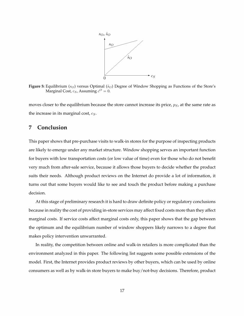
Figure 5 illustrates Result 4 by showing how the equilibrium and optimal fractions of window

shoppers among buyers who do not incur transportation costs vary with the store’s marginal cost,

cS .

The intuition behind Result 4 is as follows. If the walk-in store and the online seller have the

same marginal cost, Result 2 shows that any degree of window shopping is excessive because the

store provides after-sale service that the online seller does not offer. However, equation (21) shows

that as the store’s marginal cost increases, some window shopping is optimal because the online

seller bears a relatively lower marginal cost. Hence, the optimal degree of window shopping

16

6

- cS

sO

sO

sO, sO

0

Figure 5: Equilibrium (sO) versus Optimal (sO) Degree of Window Shopping as Functions of the Store’sMarginal Cost, cS , Assuming cO = 0.

moves closer to the equilibrium because the store cannot increase its price, pS , at the same rate as

the increase in its marginal cost, cS .

7 Conclusion

This paper shows that pre-purchase visits to walk-in stores for the purpose of inspecting products

are likely to emerge under any market structure. Window shopping serves an important function

for buyers with low transportation costs (or low value of time) even for those who do not benefit

very much from after-sale service, because it allows those buyers to decide whether the product

suits their needs. Although product reviews on the Internet do provide a lot of information, it

turns out that some buyers would like to see and touch the product before making a purchase

decision.

At this stage of preliminary research it is hard to draw definite policy or regulatory conclusions

because in reality the cost of providing in-store services may affect fixed costs more than they affect

marginal costs. If service costs affect marginal costs only, this paper shows that the gap between

the optimum and the equilibrium number of window shoppers likely narrows to a degree that

makes policy intervention unwarranted.

In reality, the competition between online and walk-in retailers is more complicated than the

environment analyzed in this paper. The following list suggests some possible extensions of the

model. First, the Internet provides product reviews by other buyers, which can be used by online

consumers as well as by walk-in store buyers to make buy/not-buy decisions. Therefore, product

17

review information flows both ways.7

Second, the retail industry environment is evolving in many ways. Fearing a loss of customers

to online retailers, many large brick-and-mortar retailers now offer online shopping with either

home delivery or store pickups. In addition, many online retailers offer easy returns, some offer

“free returns,” and some provide links to webpages where customers can find aftermarket service

providers in their area.8 In addition, online sellers keep introducing more and more products,

such as eyeglasses, that until recently were available only in walk-in stores. This is accomplished

by offering significant price reductions that are possible because online merchants learn how to

bypass the middlemen and shorten the supply chain.9

Another issue is taxation. Online retailers are exempt from sales tax in most states in which

they are not physically present. This cost advantage may disappear in the future if states find a

legal procedure that would force online retailers to collect the sales tax.10

Appendix A Optimal Pricing Under Fixed Costs

Section 4 relies on marginal cost pricing to compute the optimal division of consumers between

the two types of merchants. However, if the fixed costs FO and FS are taken into account, mer-

chants make losses if they charge prices equal to their marginal costs. Thus, an alternative welfare

criterion would be to look at normal (zero) profit prices. That is, this appendix computes the

lowest prices, subject to the restriction that no merchant makes a loss under these prices.11

7Buyers’ search costs are analyzed in Bakos (1997).8“The War Over Christmas,” Bloomberg Businessweek, November 5–11, 2012. In fact, Hitt and Frei (2002) find that

customers who use online banking have certain characteristics that make them potentially more profitable to commer-cial banks than the average bank customer who does not use online banking. Ofek, Katona, and Sarvary (2011) analyzethe impact of product returns on multichannel stores when customers’ ability to “touch and feel” products is importantin determining suitability.

9See a March 31, 2013 article in the New York Times entitled “E-Commerce Companies Bypass the Middlemen,”available at http://nyti.ms/Xl8sLW.

10Goolsbee (2000) estimates that people living in high sales taxes locations are significantly more likely to buyonline. Amazon now collects sales tax on behalf of California, Kansas, Kentucky, New York, North Dakota,Pennsylvania, Texas, and Washington; see, http://www.amazon.com/gp/help/customer/display.html?nodeId=468512. For an agreement between Amazon.com and the State of Massachusetts, see http://online.wsj.com/article/SB10001424127887324339204578173882410132440.html.

11A more widely used algorithm to compute second-best allocations is to compute Ramsey prices, which are theprices that would leave the sum of merchants’ profits equal to (or slightly above) zero. This idea is attributed toRamsey (1927) which looked at optimal taxation to finance a fixed government budget, but was later implementedas an algorithm to regulate prices charged by public utilities; see Brown and Sibley (1986), Laffont and Tirole (2001),

18

Substituting equations (8) and (9) into the profit functions described in equations (2) and (3),

prices associated with normal (zero) profit can be extracted from

0 = πO =NpO

[pSσ(σ + 1) + τ − pO(σ2 + 1)

]σ

− FO, and (23)

0 = πS = NpS [pO(σ + 1)− 2pSσ − τ + 2σ]− FS .

The normal-profit prices (denoted by pO and pS) extracted from (23) are long expressions. For this

reason, I display much shorter expressions of these prices by normalizing the online seller’s fixed

cost to zero. Formally, let FS ≥ FO = 0. In this case, the solution to (23) is

pO = 0 and pS =

√N(2σ − τ)−

√N(τ − 2σ)2 − 8FSσ

4σ√N

. (24)

Next, under normal profits, equation (4) implies that the number of window shoppers is

Ns0 = N(pS − pO) = NpS . Therefore, in order to examine the deviation of the normal-profit

optimum (computed in this appendix) from the first-best optimum, it is sufficient to compare

s0 = pS given in equation (24) with s0 given in equation (15). First, note that s0 → s0 as FS → 0.

Second, ∂s0/∂N < 0. From these we can conclude that the normal-profit optimum and the first-

best optimum yield similar allocations of consumers when either the fixed costs are low or there

are a large number of consumers (in which case the merchants’ fixed costs per customer become

negligible).

References

Bakos, Yanis. 1997. “Reducing Buyer Search Costs: Implications for Electronic Marketplaces.”

Management Science 43(12): 1676–1692.

Brown, Stephen, and David Sibley. 1986. The Theory of Public Utility Pricing. Cambridge University

Press.

Shy (2008), and their references. That algorithm may require a lump sum transfer from one merchant to another, sothis appendix departs from that algorithm and computes the prices that would leave each merchant with nonnegativeprofits.

19

Brynjolfsson, Erik, and Michael Smith. 2000. “Frictionless Commerce? A Comparison of Internet

and Conventional Retailers.” Management Science 46(4): 563–585.

Cao, Xinyu. 2012. “The Relationships Between E-shopping and Store Shopping in the Shopping

Process of Search Goods.” Transportation Research Part A: Policy and Practice 46(7): 993–1002.

Cao, Xinyu, Zhiyi Xu, and Frank Douma. 2012. “The Interactions Between E-shopping and Tradi-

tional In-store Shopping: An Application of Structural Equations Model.” Transportation 39(5):

957–974.

Carbajo, Jose, David De Meza, and Daniel J Seidmann. 1990. “A Strategic Motivation for Com-

modity Bundling.” Journal of Industrial Economics 283–298.

Cox, Anthony, Dena Cox, and Ronald Anderson. 2005. “Reassessing the Pleasures of Store Shop-

ping.” Journal of Business Research 58(3): 250–259.

Farag, Sendy, Kevin Krizek, and Martin Dijst. 2006. “E-shopping and Its Relationship with In-

store Shopping: Empirical Evidence From the Netherlands and the USA.” Transport Reviews

26(1): 43–61.

Farag, Sendy., Tim Schwanen, Martin Dijst, and Jan Faber. 2007. “Shopping Online and/or In-

store? A Structural Equation Model of the Relationships between E-shopping and In-store

Shopping.” Transportation Research Part A: Policy and Practice 41(2): 125–141.

Forman, Chris, Anindya Ghose, and Avi Goldfarb. 2009. “Competition Between Local and Elec-

tronic Markets: How the Benefit of Buying Online Depends on Where You Live.” Management

Science 55(1): 47–57.

Friberg, Richard, Mattias Ganslandt, and Mikael Sandstrom. 2001. “Pricing Strategies in E-

Commerce: Bricks vs. Clicks.” Research Institute of Industrial Economics (IFN) Working Paper.

Gabszewicz, J.Jaskold, and J.-F. Thisse. 1979. “Price Competition, Quality and Income Disparities.”

Journal of Economic Theory 20(3): 340–359.

20

Goolsbee, Austan. 2000. “In a World Without Borders: The Impact of Taxes on Internet Com-

merce.” Quarterly Journal of Economics 115(2): 561–576.

Hitt, Lorin, and Frances Frei. 2002. “Do Better Customers Utilize Electronic Distribution Channels?

The Case of PC Banking.” Management Science 48(6): 732–748.

Horn, Henrik, and Oz Shy. 1996. “Bundling and International Market Segmentation.” International

Economic Review 37(1): 51–69.

Jarboe, Glen, and Carl McDaniel. 1987. “A Profile of Browsers in Regional Shopping Malls.”

Journal of the Academy of Marketing Science 15(1): 46–53.

Laffont, Jean-Jacques, and Jean Tirole. 2001. Competition in Telecommunications. MIT press.

Ofek, Elie, Zsolt Katona, and Miklos Sarvary. 2011. ““Bricks and Clicks”: The Impact of Product

Returns on the Strategies of Multichannel Retailers.” Marketing Science 30(1): 42–60.

Ramsey, Frank. 1927. “A Contribution to the Theory of Taxation.” The Economic Journal 47–61.

Shaked, Avner, and John Sutton. 1982. “Relaxing Price Competition Through Product Differentia-

tion.” Review of Economic Studies 49(1): 3–13.

Shin, Jiwoong. 2007. “How Does Free Riding on Customer Service Affect Competition?” Marketing

Science 26(4): 488–503.

Shy, Oz. 2008. How to Price: A Guide to Pricing Techniques and Yield Management. Cambridge Uni-

versity Press.

21