interest rate risk finance 129. review of key factors impacting interest rate volatility federal...
TRANSCRIPT

Interest Rate Risk
Finance 129

Review of Key Factors Impacting Interest Rate Volatility
Federal Reserve and Monetary PolicyDiscount WindowReserve RequirementsOpen Market Operations
New Liquidity FacilitiesQuantitative EasingOperation Twist

Total Assets of Federal Reserve
www.federalreserve.gov/monetarypolicy/bst_recenttrends.htmwww.federalreserve.gov/monetarypolicy/bst_recenttrends.htm

Federal Reserve Assets - Detailed
www.federalreserve.gov/releases/h41www.federalreserve.gov/releases/h41

Current Balance Sheet Sept 2011

Review of Key Factors Impacting Interest Rate Volatility
Fisher model of the Savings MarketTwo main participants: Households and BusinessHouseholds supply excess funds to Businesses who are short of fundsThe Saving or supply of funds is upward sloping (saving increases as interest rates increase)The investment or demand for funds is downward sloping (demand for funds decease as interest rates increase)

Saving and Investment Decisions
Saving DecisionMarginal Rate of Time PreferenceTrading current consumption for future consumptionExpected InflationIncome and wealth effectsGenerally higher income – save moreFederal Government Money supply decisionsBusinessShort term temporary excess cash.Foreign Investment

Borrowing Decisions
Borrowing DecisionMarginal Productivity of CapitalExpected InflationOther

Equilibrium in the Market
Original EquilibriumS
S
S
S’
Decrease in Income
Increase in Marg. Prod Cap
D
DD’
D
Increase in Inflation Exp.
S
DD’
S’

Loanable Funds Theory
Expands suppliers and borrowers of funds to include business, government, foreign participants and households.Interest rates are determined by the demand for funds (borrowing) and the supply of funds (savings).Very similar to Fisher in the determination of interest rates, except the markets for the supply and demand for funds is expanded.

Loanable Funds
Now equilibrium extends through all markets – money markets, bonds markets and investment market. Inflation expectations can also influence the supply of funds.

Liquidity Preference Theory
Liquidity PreferenceTwo assets, money and financial assets
Equilibrium in one implies equilibrium in other
Supply of Money is controlled by Central Bank and is not related to level of interest rates (A vertical line)

The Yield Curve
Three things are observed empirically concerning the yield curve:Rates across different maturities move togetherMore likely to slope upwards when short term rates are historically low, sometimes slope downward when short term rates are historically highThe yield curve usually slope upward

Three Explanations of the Yield Curve
The Expectations Theories
Segmented Markets Theory
Preferred Habitat Theory

Pure Expectations Theory
Long term rates are a representation of the short term interest rates investors expect to receive in the future. (forward rates reflect the future expected rate).Assumes that bonds of different maturities are perfect substitutesIn other words, the expected return from holding a one year bond today and a one year bond next year is the same as buying a two year bond today.
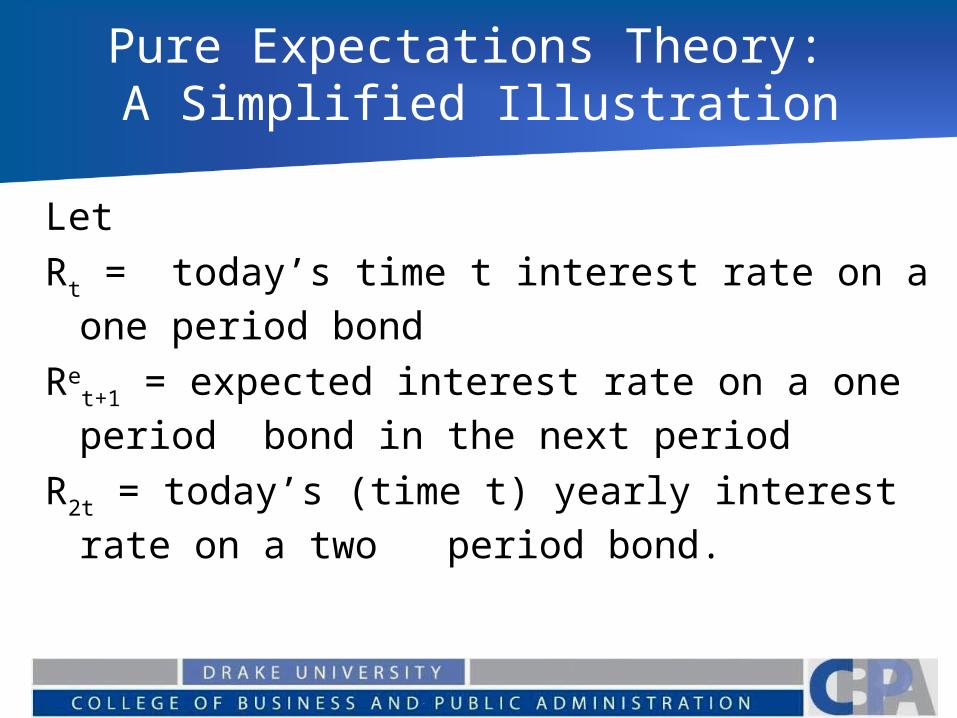
Pure Expectations Theory: A Simplified Illustration
LetRt = today’s time t interest rate on a one
period bondRe
t+1 = expected interest rate on a one period bond in the next period
R2t = today’s (time t) yearly interest rate on a two period bond.

Investing in successive one period bonds
If the strategy of buying the one period bond in two consecutive years is followed the return is:
(1+Rt)(1+Ret+1) – 1 which equals
Rt+Ret+1+ (Rt)(R
et+1)
Since (Rt)(Ret+1) will be very small we will ignore it
that leavesRt+Re
t+1
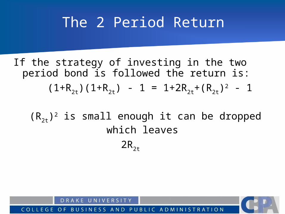
The 2 Period Return
If the strategy of investing in the two period bond is followed the return is:
(1+R2t)(1+R2t) - 1 = 1+2R2t+(R2t)2 - 1
(R2t)2 is small enough it can be dropped
which leaves
2R2t

Set the two equal to each other
2R2t = Rt+Ret+1
R2t = (Rt+Ret+1)/2
In other words, the two period interest rate is the average of the two one period rates

Expectations Hypothesis R2t = (Rt+Re
t+1)/2
Fact 1 and Fact 2 are explained well by the expectations hypothesis
However it does not explain Fact 3, that the yield curve usually slopes up.

Problems with Pure Expectations
The pure expectations theory ignores the fact that there is reinvestment rate risk and different price risk for the two maturities.Consider an investor considering a 5 year horizon with three alternatives:
buying a bond with a 5 year maturitybuying a bond with a 10 year maturity and holding it 5 yearsbuying a bond with a 20 year maturity and holding it 5 years.

Price Risk
The return on the bond with a 5 year maturity is known with certainty the other two are not.
The longer the maturity the greater the price risk

Reinvestment rate risk
Now assume the investor is considering a short term investment then reinvesting for the remainder of the five years or investing for five years.
Again the 5 year return is known with certainty, but the others are not.

Cox, Cox, Ingersoll, and Ross 1981 Journal of FinanceIngersoll, and Ross 1981 Journal of Finance
Local Expectations
Similarly owning the bond with each of the longer maturities should also produce the same 6 month return of 2%.The key to this is the assumption that the forward rates hold. It has been shown that this interpretation is the only one that can be sustained in equilibrium.*

Return to maturity expectations hypothesis
This theory claims that the return achieved by buying short term and rolling over to a longer horizon will match the zero coupon return on the longer horizon bond. This eliminates the reinvestment risk.

Expectations Theory and Forward Rates
The forward rate represents a “break even” rate since it the rate that would make you indifferent between two different maturitiesThe pure expectations theory and its variations are based on the idea that the forward rate represents the market expectations of the future level of interest rates.However the forward rate does a poor job of predicting the actual future level of interest rates.

Segmented Markets Theory
Interest Rates for each maturity are determined by the supply and demand for bonds at each maturity.Different maturity bonds are not perfect substitutes for each other.Implies that investors are not willing to accept a premium to switch from their market to a different maturity.Therefore the shape of the yield curve depends upon the asset liability constraints and goals of the market participants.

Biased Expectations Theories
Both Liquidity Preference Theory and Preferred Habitat Theory include the belief that there is an expectations component to the yield curve.Both theories also state that there is a risk premium which causes there to be a difference in the short term and long term rates. (in other words a bias that changes the expectations result)

Liquidity Preference Theory
This explanation claims that the since there is a price risk and liquidity risk associated with the long term bonds, investor must be offered a premium to invest in long term bonds Therefore the long term rate reflects both an expectations component and a risk premium.The yield curve will be upward sloping as long as the premium is large.
Preferred Habitat Theory
Like the liquidity theory this idea assumes that there is an expectations component and a risk premium.In other words the bonds are substitutes, but savers might have a preference for one maturity over another (they are not perfect substitutes).However the premium associated with long term rates does not need to be positive. If there are demand and supply imbalances then investors might be willing to switch to a different maturity if the premium produces enough benefit.

Preferred Habitat Theoryand The 3 Empirical Observations
The biased expectation theories can explain all three empirical facts.

Yield Curves Feb 2012 – Aug 2012
data from www.ustreas.govdata from www.ustreas.gov
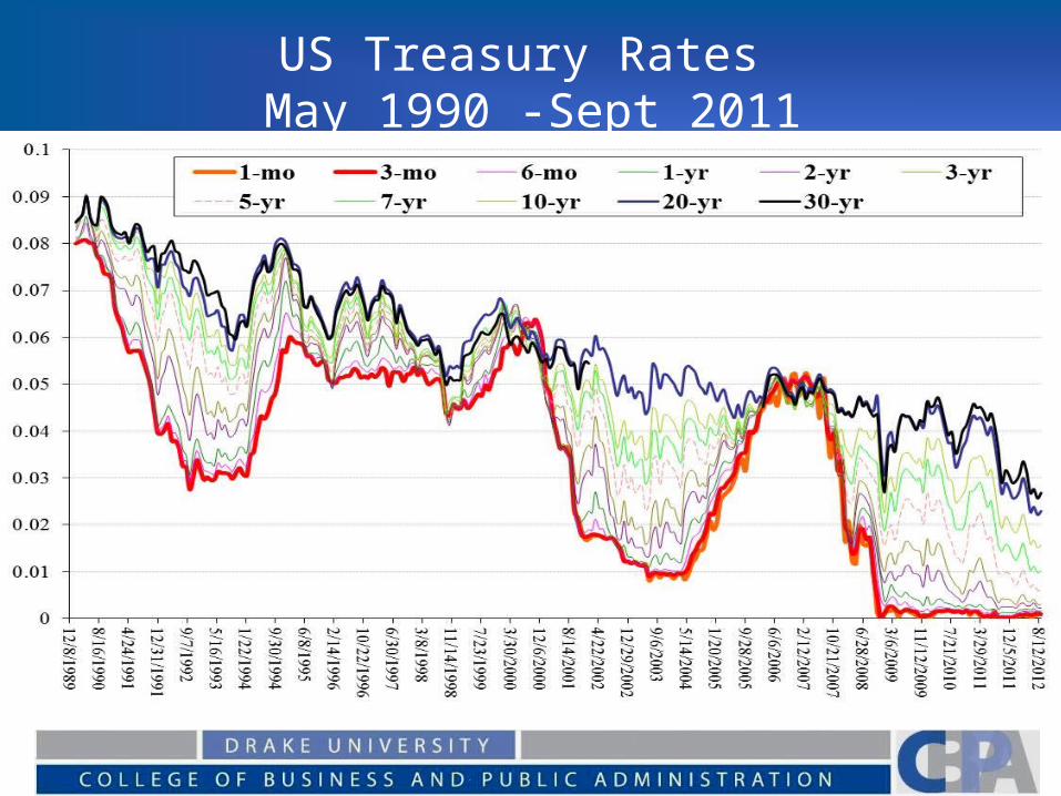
US Treasury Rates May 1990 -Sept 2011
data from www.ustreas.govdata from www.ustreas.gov

Maturity Yield Spreads1990 - 2011
data from www.ustreas.gov

Impact of Interest Rate Volatility on Financial Institutions
The market value of assets and liabilities is tied to the level of interest ratesInterest income and expense are both tied to the level of interest rates

Static GAP Analysis(The repricing model)
Repricing GAPThe difference between the value of interest sensitive assets and interest sensitive liabilities of a given maturity. Measures the amount of rate sensitive assets and liabilities (asset or liability will be repriced to reflect changes in interest rates) for a given time frame.

Commercial Banks & GAP
Commercial banks are required to report quarterly the repricing Gaps for the following time frames
One dayMore than one day less than 3 monthsMore than 3 months, less than 6 monthsMore than 6 months, less than 12 monthsMore than 12 months, less than 5 yearsMore than five years
GAP Analysis
Static GAP-- Goal is to manage interest rate income in the short run (over a given period of time)
Measuring Interest rate risk – calculating GAP over a broad range of time intervals provides a better measure of long term interest rate risk.

Interest Sensitive GAP
Given the Gap it is easy to investigate the change in the net interest income of the financial institution.
sLiabilitie Sensistive Rate - Assets Sensistive Rate GAP
R)(GAP)( NII
Rates)in ge(GAP)(Chan NIIin Change

Example
Over next 6 Months:Rate Sensitive Liabilities = $120 million
Rate Sensitive Assets = $100 Million
GAP = 100M – 120M = - 20 Million
If rate are expected to decline by 1%Change in net interest income
= (-20M)(-.01)= $200,000

GAP Analysis
Asset sensitive GAP (Positive GAP)RSA – RSL > 0If interest rates NII will If interest rates NII will
Liability sensitive GAP (Negative GAP)RSA – RSL < 0If interest rates NII will If interest rates NII will
Would you expect a commercial bank to be asset or liability sensitive for 6 mos? 5 years?

Important things to note:
Assuming book value accounting is used -- only the income statement is impacted, the book value on the balance sheet remains the same.
The GAP varies based on the bucket or time frame calculated.
It assumes that all rates move together.
Steps in Calculating GAP
1) Select time Interval
2) Develop Interest Rate Forecast
3) Group Assets and Liabilities by the time interval (according to first repricing)
4) Forecast the change in net interest income.

Alternative measures of GAP
Cumulative GAPTotals the GAP over a range of of possible maturities (all maturities less than one year for example).Total GAP including all maturities

Other useful measures using GAP
Relative Interest sensitivity GAP (GAP ratio)GAP / Bank SizeThe higher the number the higher the risk that is present
Interest Sensitivity Ratio
SensitiveAsset 1
SensitiveLiability 1
sLiabilitieSensitive Rate
Assets Sensitive Rate

What is “Rate Sensitive”
Any Asset or Liability that matures during the time frameAny principal payment on a loan is rate sensitive if it is to be recorded during the time periodAssets or liabilities linked to an indexInterest rates applied to outstanding principal changes during the interval
What about Core Deposits?
Against InclusionDemand deposits pay zero interestNOW accounts etc do pay interest, but the rates paid are sticky
For InclusionImplicit costsIf rates increase, demand deposits decrease as individuals move funds to higher paying accounts (high opportunity cost of holding funds)

Expectations of Rate changes
If you expect rates to increase would you want GAP to be positive or negative?
Positive – the increase in assets > increase in liabilities so net interest income will increase.

Unequal changes in interest rates
So far we have assumed that the change the level of interest rates will be the same for both assets and liabilities.If it isn’t you need to calculate GAP using the respective change.Spread effect – The spread between assets and liabilities may change as rates rise or decrease
)R(RSL)(-)R(RSA)( NII liabiltiesassets

Strengths of GAP
Easy to understand and calculate
Allows you to identify specific balance sheet items that are responsible for risk
Provides analysis based on different time frames.

Weaknesses of Static GAP
Market Value EffectsBasic repricing model the changes in market value. The PV of the future cash flows should change as the level of interest rates change. (ignores TVM)
Over aggregationRepricing may occur at different times within the bucket (assets may be early and liabilities late within the time frame)Many large banks look at daily buckets.

Weaknesses of Static GAP
RunoffsPeriodic payment of principal and interest that can be reinvested and is itself rate sensitive.You can include runoff in your measure of rate sensitive assets and rate sensitive liabilities.Note: the amount of runoffs may be sensitive to rate changes also (prepayments on mortgages for example)

Weaknesses of GAP
Off Balance Sheet ActivitiesBasic GAP ignores changes in off balance sheet activities that may also be sensitive to changes in the level of interest rates.
Ignores changes in the level of demand deposits

Other Factors Impacting NII
Changes in Portfolio CompositionAn aggressive position is to change the portfolio in an attempt to take advantage of expected changes in the level of interest rates. (if rates are have positive GAP, if rates are have negative GAP)Problem: Forecasting is rarely accurate

Other Factors Impacting NII
Changes in VolumeBank may change in size so can GAP along with it.
Changes in the relationship between ST and LTWe have assumes parallel shifts in the yield curve. The relationship between ST and LT may change (especially important for cumulative GAP)

Extending Basic GAP
You can repeat the basic GAP analysis and account for some of the problemsInclude
Forecasts of when embedded options will be exercised and include themInclude off balance sheet itemsRecalculate across different interest rate assumptions (and repricing assumptions)

The Maturity Model
In this model the impact of a change in interest rates on the market value of the asset or liability is taken into account.The securities are marked to marketKeep in Mind the following:
The longer the maturity of a security the larger the impact of a change in interest ratesAn increase in rates generally leads to a fall in the value of the securityThe decrease in value of long term securities increases at a diminishing rate for a given increase in rates

Weighted Average Maturity
You can calculate the weighted average maturity of a portfolio. The same three principles of the change in the value of the portfolio (from last slide) will apply
ininiiiii MWMWMWM 2211

Maturity GAP
Given the weighted average maturity of the assets and liabilities you can calculate the maturity GAP
sliabilitieassets M MMGap

Maturity Gap Analysis
If Mgap is + the maturity of the FI assets is longer than the maturity of its liabilities. (generally the case with depository institutions due to their long term fixed assets such as mortgages).This also implies that its assets are more rate sensitive than its liabilities since the longer maturity indicates a larger price change.

The Balance Sheet and MGap
The basic balance sheet identity state that:Asset = Liabilities + Owners Equity orOwners Equity = Assets - Liabilities
Technically if Liab >Assets the institution is insolvent
If MGAP is positive and interest rate decrease then the market value of assets increases more than liabilities and owners equity increases.Likewise, if MGAP is negative an increase in interest rates would cause a decrease in owners equity.

Matching Maturity
By matching maturity of assets and liabilities owners can be immunized form the impact of interest rate changes.However this does not always completely eliminate interest rate risk. Think about duration and funding sources (does the timing of the cash flows match?).

Duration
Duration: Weighted maturity of the cash flows (either liability or asset)Weight is a combination of timing and magnitude of the cash flowsThe higher the duration the more sensitive a cash flow stream is to a change in the interest rate.

Duration MathematicsBond Example
Taking the first derivative of the bond value equation with respect to the yield will produce the approximate price change for a small change in yield.

Duration Mathematics
1n1n432 r)(1
(-n)MV
r)(1
(-n)CP
r)(1
(-3)CP
r)(1
(-2)CP
r)(1
(-1)CP
r
P
nn32 r)(1
MV
r)(1
CP
r)(1
CP
r)(1
CP
r)(1
CPP
nn32 r)(1
nMV
r)(1
nCP
r)(1
3CP
r)(1
2CP
r)(1
1CP
r1
1
r
P
The approximate price change for a small change in r
Duration Mathematics
nn32 r)(1
nMV
r)(1
nCP
r)(1
3CP
r)(1
2CP
r)(1
1CP
r1
1
r
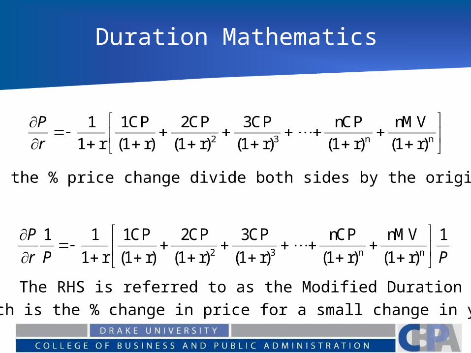
P
To find the % price change divide both sides by the originalPrice
PPr
P 1
r)(1
nMV
r)(1
nCP
r)(1
3CP
r)(1
2CP
r)(1
1CP
r1
11nn32
The RHS is referred to as the Modified DurationWhich is the % change in price for a small change in yield

Duration MathematicsMacaulay Duration
Macaulay Duration is the price elasticity of the bond (the % change in price for a percentage change in yield).Formally this would be:
P
r)(1
price Original
yield Original
Yieldin Change
Pricein Change
yield originalyieldin change
price originalpricein change
DMAC
r
P

Duration MathematicsMacaulay Duration
P
r)(1
price Original
yield Original
Yieldin Change
Pricein Change
yield originalyieldin change
price originalpricein change
DMAC
r
P
nn32 r)(1
nMV
r)(1
nCP
r)(1
3CP
r)(1
2CP
r)(1
1CP
r1
1
r
P
substitutesubstitute
P
r)(1
r)(1
nMV
r)(1
nCP
r)(1
3CP
r)(1
2CP
r)(1
1CP
r1
1nn32
MACD

Macaulay Duration of a bond
N
1tNt
N
1tNt
r)(1MV
r)(1CP
r)(1N(MV)
r)(1t(CP)
MACD
P
1
r)(1
nMV
r)(1
nCP
r)(1
3CP
r)(1
2CP
r)(1
1CPnn32
MACD

Duration Example
10% 30 year coupon bond, current rates =12%, semi annual payments
periods 3895.17
)06.1(1000$
)06.1(50
)06.1()1000($60
)06.1()50($
60
160
60
160
tt
tt
MAC
t
D

Example continued
Since the bond makes semi annual coupon payments, the duration of 17.3895 periods must be divided by 2 to find the number of years.17.3895 / 2 = 8.69475 yearsThis interpretation of duration indicates the average time taken by the bond, on a discounted basis, to pay back the original investment.

Using Duration to estimate price changes
P
r)(1DMAC
r
P
r)(1
rDMAC
P
PRearrange
% Change in Price
Estimate the % price change for a 1 basis point increase in yield
000776.012.1
0001.69925.8
r)(1
rDMAC
P
P
The estimated price change is then
-0.000776(838.8357)=-0.6515

Using Duration Continued
Using our 10% semiannual coupon bond, with 30 years to maturity and YTM = 12%Original Price of the bond = 838.3857If YTM = 12.01% the price is 837.6985
This implies a price change of -0.6871Our duration estimate was -0.6515

Modified Duration
PPr
P 1
r)(1
nMV
r)(1
nCP
r)(1
3CP
r)(1
2CP
r)(1
1CP
r1
11nn32
From before, modified duration was defined as
Macaulay Duration
r)(1
DurationMacaulay
Duration
Modified

Modified Duration
000776.012.1
0001.69925.8
r)(1
rDMAC
P
P
r)(1
DurationMacaulay
Duration
Modified
Using Macaulay Duration
000776.0)0001(.12.1
69925.8
rDrr)(1
D
r)(1
rD MODIFIED
MACMAC
P
P

Duration
Keeping other factors constant the duration of a bond will:Increase with the maturity of the bondDecrease with the coupon rate of the bondWill decrease if the interest rate is floating making the bond less sensitive to interest rate changesDecrease if the bond is callable, as interest rates decrease (increasing the likelihood of call) duration increases

Duration and Convexity
Using duration to estimate the price change implies that the change in price is the same size regardless of whether the price increased or decreased.The price yield relationship shows that this is not true.

Duration and Convexity
0
500
1000
1500
2000
2500
3000
0 0.05 0.1 0.15 0.2
Interest Rate
Bo
nd
Valu
e

Duration and Yield Changes
Duration provides a linear approximation of the price change associated with a change in yield. The duration of an asset will change depending upon the original yield used in its calculation. As the yield decreases, the price change associated with a change in yield increases.Likewise duration will increase as the yield of an option free bond decreases. This is illustrated as a steeper line approximately tangent to the price yield relationship.

0
500
1000
1500
2000
2500
3000
3500
0 0.02 0.04 0.06 0.08 0.1 0.12 0.14
Impact of yield on Duration Estimate of Price change

0
500
1000
1500
2000
2500
3000
3500
0 0.05 0.1 0.15 0.2 0.25 0.3
Change in duration outlines the price yield relationship

0
500
1000
1500
2000
2500
3000
3500
0 0.05 0.1 0.15 0.2 0.25
Duration and the Convexity of the Price - Yield Relationship

0
500
1000
1500
2000
2500
3000
3500
0 0.05 0.1 0.15 0.2 0.25
Duration and the Convexity of the Price - Yield Relationship

Basic Duration Gap
Duration Gap
DLDADGAP Basic
PortfolioLibaility of
Duration Weighted$
PortfolioAsset of
Duration Weighted$ DGAP Basic

Basic DGAP Conintued
iasset ofDuration Macaulay DaAssets All of ValueMarket
Asset wwhere
DawDAPortfolioAsset of
Duration Weighted$
i
ii
i
N
1ii
jLiability ofDuration Macaulay DlsLiabilitie All of ValueMarket
Asset wwhere
DlwDLPortfolioLiability of
Duration Weighted$
j
jj
j
N
1jj

Basic DGAP
If the Basic DGAP is +If Rates in the value of assets > in value of liabOwners equity will decreaseIf Rate
in the value of assets > in value of liabOwners equity will increase

Basic DGAP
If the Basic DGAP is (-)If Rates in the value of assets < in value of liabOwners equity will increaseIf Rate
in the value of assets < in value of liabOwners equity will decrease

Basic DGAP
Does that imply that if DA = DL the financial institution has hedged its interest rte risk?
No, because the $ amount of assets > $ amount of liabilities otherwise the institution would be insolvent.

DGAP
Let MVL = market value of liabilities and MVA = market value of assetsThen to immunize the balance sheet we can use the following identity:
MVA
MVLDLDADGAP
MVA
MVLDLDA

DGAP and equity
Let MVE = MVA – MVLWe can find MVA & MVL using duration
From our definition of duration:
MVLy1
Δy-DL MVL
MVA y1
Δy-DAMVA
formula theApplying Pi)(1
ΔiDΔP

MVAy1
Δy-DGAPΔMVE
MVAy1
Δy
MVA
MVL(DL)- (DA)-
y1
Δy(DL)MVL-(DA)MVA -
MVLy1
ΔyDL--MVA
y1
Δy-DA
ΔMVL-ΔMVA ΔMVE

DGAP Analysis
If DGAP is (+)An in rates will cause MVE to An in rates will cause MVE to
If DGAP is (-)An in rates will cause MVE to An in rates will cause MVE to
The closer DGAP is to zero the smaller the potential change in the market value of equity.

Weaknesses of DGAP
It is difficult to calculate duration accurately (especially accounting for options)Each CF needs to be discounted at a distinct rate can use the forward rates from treasury spot curveMust continually monitor and adjust durationIt is difficult to measure duration for non interest earning assets.

More General Problems
Interest rate forecasts are often wrongTo be effective management must beat the ability of the market to forecast rates
Varying GAP and DGAP can come at the expense of yield
Offer a range of products, customers may not prefer the ones that help GAP or DGAP – Need to offer more attractive yields to entice this – decreases profitability.

Duration in Practice
Impact of convexityShape of the yield curveDefault RiskFloating Rate InstrumentsDemand DepositsMortgagesOff Balance Sheet items

Convexity Revisited
The more convexity the asset or portfolio has, the more protection against rate increases and the greater the possible gain for interest rate falls.The greater the convexity the greater the error possible if simple duration is calculated.All fixed income securities have convexityThe larger the change in rates, the larger the impact of convexity
Flat Term Structure
Our definition of duration assumes a flat term structure and that the all shirts in the yield curve are parallel. Discounting using the spot yield curve will provide a slightly different measure of inflation.

Default Risk
Our measures assume that the risk of default is zero. Duration can be recalculated by replacing each cash flow by the expected cash flow which includes the probability that the cash flow will be received.

Floating Rates
If an asset or liability carries a floating interest rate it readjusts its payments so the future cash flows are not known.Duration is generally viewed as being the time until the next resetting of the interest rate.

Demand Deposits
Deposits have an open ended maturity. You need to define the maturity to define duration. Method 1
Look at turnover of deposits (or run). If deposits turn over 5 times a year then they have an average maturity of 73 days (365/5).
Method 2Think of them as a puttable bond with a duration of 0
Method 3Look at the % change in demand deposits for a given level of interest rate changes.
Simulation
Mortgages
Mortgages and mortgage backed securities have prepayment risk associated with them. Therefore we need to model the prepayment behavior of the mortgage to understand the cash flow.

Off Balance Sheet Items
The value of derivative products also are impacted by duration changes. They should be included in any portfolio duration estimate or GAP analysis.