wind turbine noise source characteristics measured with a ... · stuart bradley (a), torben...

Buenos Aires – 5 to 9 September, 2016 Acoustics for the 21st Century…

PROCEEDINGS of the 22nd International Congress on Acoustics

Wind Farm Noise: Paper ICA2016-565

Wind turbine noise source characteristics measured with a large microphone array

Stuart Bradley(a), Torben Mikkelsen(b), Sabine von Hünerbein(c), Mathew Legg(d) (a) University of Auckland, New Zealand, [email protected]

(b) Technical University of Denmark, Denmark, [email protected] (c) University of Salford, UK, [email protected]

(d) University of Auckland, New Zealand, [email protected]

Abstract

A large 40 m scale microphone array was designed to record the noise from a wind turbine. The objective was to acoustically image the noise source characteristics across the entire diameter of the turbine at a spatial resolution of 1 m at 1/3 octave resolution. This allows simultaneous definition of the spatial, temporal, and spectral properties of the generated sound. The array comprised 42 purpose-designed low-noise microphones simultaneously sampled at 20 kHz. Very high quality, fast, meteorological profile data was available from nearby 80 m masts and from the turbine nacelle, giving wind speed, wind direction, and turbulence data. A speaker was mounted at the base of the turbine tower, for determining the spatial characteristics of coherence, and for compensating for local wind variations. An experiment was also run recording the sound from a continuous tone speaker mounted near the tip of a turbine blade, allowing testing of signal processing to correct for the very substantial Doppler shift. We describe the significant challenges in imaging with such a large array. High resolution image results are given as well as time-resolved and spectrally-resolved turbine noise directivity patterns.

Keywords: wind turbine noise, wind turbine amplitude modulation, microphone array, wind turbine noise source characteristics

22nd International Congress on Acoustics, ICA 2016 Buenos Aires – 5 to 9 September, 2016

Acoustics for the 21st Century…

2

Wind turbine noise source characteristics measured with a large microphone array

1 Introduction Particularly over the past decade noise from wind turbines has become a major concern for the public, and therefore for the industry. In addition to broad-band noise, generally identified as trailing edge noise, there has been an increasing concern about the annoyance to people by amplitude modulation (AM) of wind turbine noise [1] A study by RenewableUK [2] provides wide cover of different aspects of AM and the more extreme version of modulation named “other amplitude modulation” (OAM). The main hypothesis for the cause of OAM in the RenewableUK study has been that it is due to intermittent stall of a blade. Oerlemans [3] developed a rotor simulation model including a noise model for a partially stalled airfoil and the model results showed the general observed characteristics of OAM. The source directivity characteristics of the stall noise are such that it is preferentially radiated upwind and downwind of the wind turbine and not in the cross wind direction as characterizes AM.

More recently, Madsen et al., [4] have correlated AM with turbine blade inflow conditions. They found a strong noise increase at low frequencies when a trailing edge stall initiates. For the turbine operating in a strong wind shear a modulation of the surface spectra for frequencies below 200Hz is 14dB. It was hypothesised that coupling with the turbine wake can cause abrupt changes in wind speed over the rotor disc and for a variable speed turbine the rotor might not be able to accelerate fast enough to avoid transient stall for a few revolutions. This intermittent occurrence might explain many of the occurrences of OAM.

Given the uncertainties still around the mechanisms, as series of experiments were conducted on a turbine at the DTU Roskilde campus in Denmark. The objective was to obtain detailed spatial and spectral information on the origins of the turbine noise using an imaging array of microphones situated on the flat ground behind the turbine. The reason for this approach was to separate the sound generating mechanisms from sound propagation, and also to do this in the far field of the sound, rather than on the turbine blade itself, so that all emitted sound was included in appropriate phase and so that the very substantial Doppler shift was measured.

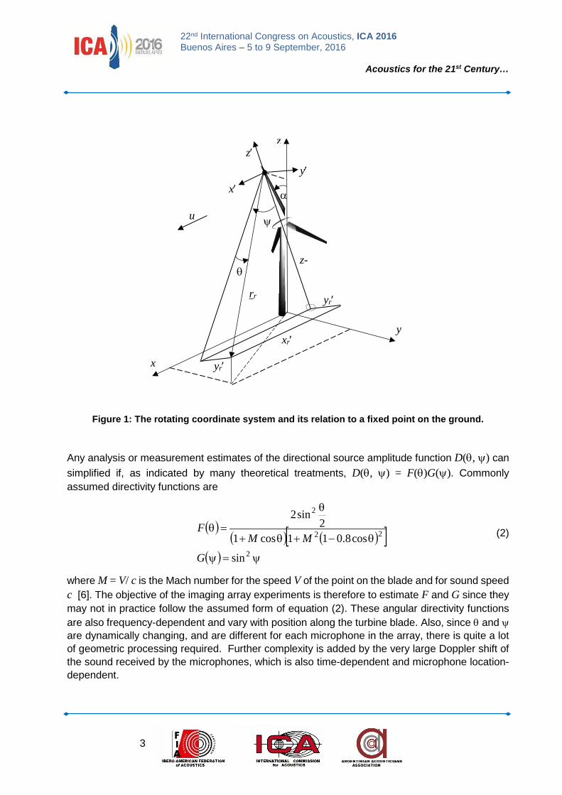
The directivity of the sound from the turbine is fixed with respect to the rotating turbine blades (see, for example, [5]), assuming a fixed angle of attack. It therefore makes sense to use a rotor-centred coordinate system shown in Figure 1.

The wind of uniform speed u is in the x direction and the rotor is turning with angular frequency Ω so that α = Ωt, where t is time measured from when the turbine is at the top of its sweep. The fixed measurement point on the ground subtends an angle ψ to the blade in the plane of the blade and the wind, and an angle θ perpendicular to this plane, as shown below, and where

( )r

r

r

rr

zx

yzx

′′

=ψ′′+′

=θ tantan2/122

. (1)



3

z

y

x

α

z′

rr

u

x′ y′

z-

xr′

yr′

ψ

yr′

θ

Figure 1: The rotating coordinate system and its relation to a fixed point on the ground.

Any analysis or measurement estimates of the directional source amplitude function D(θ, ψ) can simplified if, as indicated by many theoretical treatments, D(θ, ψ) = F(θ)G(ψ). Commonly assumed directivity functions are

( )( ) ( )[ ]

( ) ψ=ψ

θ−+θ+

θ

=θ

2

22

2

sin

cos8.011cos12

sin2

G

MMF (2)

where M = V/ c is the Mach number for the speed V of the point on the blade and for sound speed c [6]. The objective of the imaging array experiments is therefore to estimate F and G since they may not in practice follow the assumed form of equation (2). These angular directivity functions are also frequency-dependent and vary with position along the turbine blade. Also, since θ and ψ are dynamically changing, and are different for each microphone in the array, there is quite a lot of geometric processing required. Further complexity is added by the very large Doppler shift of the sound received by the microphones, which is also time-dependent and microphone location-dependent.



4

2 The microphone array 2.1 Spatial resolution and array size In practice the source may be distributed or there may be multiple sources and/or noise from, for example, traffic. This means the microphone array should ideally have sensitivity primarily in a narrow solid angle. If the microphones are regularly spaced, then diffraction grating effects emerge, where multiple diffraction orders produce strong sensitivity in directions other than the array axis. This can be avoided by closely spacing the microphones, but then a very large number of microphones is generally needed since the overall array diameter determines the angular resolution achieved. For this reason the microphone array needs to have microphone spacings which are unique (a ‘non-redundant’ array design). Successful designs generally have the microphones placed on multiple spiral paths, with the microphone spacing along the spiral path varying with distance from the array centre.

A study by Prime et al. [7] concluded that the Underbrink array performed best overall, and that basic design is also used here. Firstly, the scale of the array (i.e. its diameter Da) needs to be chosen. The spatial resolution is diffraction-limited by the diameter of the array and, if it was far-field Airy diffraction with the turbine on the axis of the array, the 3 dB spatial resolution at the turbine would be roughly 0.35 dc/(fDa) = 119 (d/Da)/f where c is the sound speed and f = ω/(2π) the source frequency. Choosing Da = 20 m gives a resolution of 1 m if d = 100 m, and f = 600 Hz. Secondly, the array is in the plane of the ground whereas the noise source is in the rotor plane, so the array axis is not directed toward the source. The angular dimensions of the array, as seen from the source, also change with rotor angle. If the array is stretched in the x direction to be elliptical, with the major axis along the x axis, then the array shape as seen from the source can be made more circular. The projected array shape is found by taking lines from the source to the array perimeter, and projecting these onto the plane which is normal to the line joining the source and the array centre and which passes through the array centre. At any particular rotor angle this procedure gives an axial ratio for the array circumference, as seen from the source on the rotor blade. These projected axial ratios are shown in Figure 2 for a selection of elliptical array shapes. The projection is onto the plane which is perpendicular to the line from the source to the array centre. The elliptical array has axial ratio of cosβ.

It can be seen that the projected view from the turbine cannot be corrected to be a circular shape for all rotor positions, but if the array shape on the ground is stretched to have an axial ratio of cos(57.5°), then the projected elliptical shape will vary between axial ratios of 10-0.15 to 10+0.15 or 1/1.4 to 1.4. This can be expected to give a variation in the vertical and horizontal resolution with position of the rotor blade.

Figure 3 shows an Underbrink array design comprising six spiral arms with each arm containing seven microphones. The design has the innermost microphones at a radius of 1.4 m from the array centre, and the outermost microphones at a distance of 9.8 m. This design allows each microphone to be connected via a 20 m cable to a central data system, allowing 1.5 m extra for each cable. The rate of spiral expansion is determined by the spiral angle ν = 11π/30.



5

Figure 2: The axial ratio of the projection of a horizontal elliptical array.

2.2 Temporal resolution and sampling duration The high resolution of this large array means the sound source might move through several pixels during sampling. This can cause an incorrect impression of the source location, spectral spread, and incorrect sound pressure levels. The microphone outputs were bandlimited with a high frequency cut-off of around 6 kHz, but synchronous sampling of all 42 microphones was done at 20 kHz.

Since we are aiming to localise the sound source and also determine the directivity patterns, it is desirable to average the results, synchronised to blade position. This means that the duration of a recorded file needs to include many turbine blade passes. We chose 5-minute files as a compromise between the number of blade passes included and having a reasonably compact file for easy processing. The binary 5-minute files, containing the data for 42 microphones, have a size of about 0.85 Gb, and the associated 5-minute video clip (see below) is another 85 Mb, so each 5 minutes we record 0.93 Gb, giving around 0.3 Tb per day.

2.3 Registration Synchronously with the microphone array recording, a video recording is made of the turbine. This allows precise registration of sampled sound with the turbine blade position and speed. Synchronous averaging is possible (each average triggered from when a blade is at the highest position) which will increase the turbine noise signal in comparison with background wind and



6

traffic noise. Video output from a video camera at the center of the array is time-synchronized with the microphone data recording. The blade position is found by simple image slices, as shown in Figure 4. When the intensity peaks from two image columns align, then the blade is horizontal.

Figure 3. View of the large spiral array from near the turbine hub height (the turbine is to the

left of the camera position).

In addition, a speaker is mounted near the base of the turbine and two tones generated by the central computer, at the 1/3-octave center frequencies of 1250 Hz and 3150 Hz. These two frequencies fall within the sampled spectral range (and bandpass filter range) but lie outside the spectral are of most interest for turbine noise. The two 1/3-octave bands in which these tones lie are unusable for analysis of WTN. Two tones are used because this allows precise phase registration dynamically of each microphone, in the presence of horizontal winds. The speaker is not rotating, as the blades are, so there is no Doppler shift compensation required. The continuous use of two tones allows checking throughout the experiments on the accuracy with which the position of the speaker can be determined by the array, although the speaker is at much lower elevation compared to the rotating noise sources.

2.4 Supporting data Very high quality, fast, meteorological profile data was available from nearby 80 m masts and from the turbine nacelle, giving wind speed, wind direction, and turbulence data.



7

Figure 4. Video frame (left) and intensity from two vertical image columns (right).

3 First results 3.1 Variation with height of the microphone A microphone on the ground has the directivity pattern sweep across it as a blade turns, causing a modulation of the sound. A microphone directly behind the turbine and at hub height should have a minimal modulation because the directivity pattern is not sweeping past.

To test this idea, we used a hydraulic lift and recoded the sound for about one minute at ten heights from 13 m above ground up to 36 m. For this Nortek turbine, the hub height is H = 35 m, and the rotor blade radius is R = 20 m.

Figure 5 shows sound pressure levels in several octave bands vs height. Wind noise is generally increasing with height, but the lower frequency sound also has a peak at around 23 m. Some estimation of directivity is in principle able to be derived from these curves, making use of the known geometry at each height. The variation in directivity D over one blade rotation, based on equation (2) shows a peak at 21 m.

50 100 150 200 250 300 350 400

50

100

150

200

250

300



8

Figure 5. Sound pressure levels in several octave bands vs height

3.2 Doppler shift There is a lot of Doppler shift because of the blade motion. This frequency shift is different for each microphone. To get phase alignment, corrections have to be applied for the Doppler shift. As a demonstration experiment for assessing the Doppler shift, we mounted a 2.5 kHz speaker on one of the turbine blades, near the tip (see Figure 6). The spectrogram in Figure 6 shows the Doppler variation as the blade turns for the particular position used for recording on this occasion.

3.3 Spatial coherence The speaker mounted at the base of the turbine tower is used to determine the spatial characteristics of coherence, and for compensating for local wind variations. Figure 7 shows the maximum value of the cross-correlation between the signals in the 1250 Hz band for all pairs of microphones, as a function of microphone-microphone separation. The data are averaged over 3.5 m bins. It is clear that there is no significant fall off of correlation with distance within the diameter of the array.

4 Conclusions Tackling the problem of doing good quantitative measurements of turbine noise brings up a whole lot of challenges. A set of experiments designed to obtain precision measurements has been outlined. The data appear to be of good quality, but instrumental artefacts must be removed.



9

Figure 6. Spectrogram of the sound recorded at the ground from a speaker on the blade (inset).

Figure 7. Peak values of normalised cross correlation of signals in the 1250 Hz band.



10

Some first results are given, setting the stage for the complex microphone imaging challenges in this research program.

Since these kind of measurements have not been done before anywhere, there is strong likelihood of interesting new insights.

Acknowledgments Professor Bradley’s collaboration with DTU was funded via the Velux Foundation Visiting Professorship award for 2015, which is gratefully acknowledged.

References [1] Bowdler, D. Amplitude modulation of wind turbine noise: a review of the evidence, Institute of Acoustics

Bulletin, Vol 33 (4), 2008, pp 31–41.

[2] Bullmore, A.; Oerlemans, S.; Smith, M.; White, P.; von Hünerbein, S.; King, A; Piper, B. Wind Turbine Amplitude Modulation: Research to Improve Understanding as to its Cause and Effects. RUK, 2013.

[3] Oerlemans, S. An explanation for enhanced amplitude modulation of wind turbine noise. In RenewableUK 2013 report: Wind Turbine Amplitude Modulation: Research to Improve Understanding as to its Cause & Effect, 2013.

[4] Madsen, H.A.; Bertagnolio, F.; Fischer, A.; Bak, C. Correlation of amplitude modulation to inflow characteristics. INTER-NOISE and NOISE-CON Congress and Conference Proceedings, 12136–12136, 2014.

[5] Da Conceição Vargas, L.F. Wind turbine noise prediction. Universidad técnica de Lisboa. 2008.

[6] Bowdler, D.; Leventhall, G. Wind Turbine Noise. Multi-Science Publishing. 2011.

[7] Prime, Z.; Doolan, C.; Zajamsek, B. Beamforming array optimisation and phase averaged sound source mapping on a model wind turbine. INTER-NOISE and NOISE-CON Congress and Conference Proceedings, 1078–1086, 2014.

wind turbine noise source characteristics measured with a ... · stuart bradley (a), torben...

Documents