Using a Ventilation Controller to Optimize Residential Passive Ventilation For Energy and Indoor Air Quality

William J.N. Turner & Iain S. Walker Environmental Energy Technologies Division August 2014

LBNL XXXXX

Funding was provided by the California Energy Commission through Contract No. 500-08-061 and the U.S. Dept. of Energy under Contract No. DE-AC02-05CH11231

Disclaimer

This document was prepared as an account of work sponsored by the United States Government. It does not necessarily represent the views of the Energy Commission, its employees or the State of California. While this document is believed to contain correct information, the United States Government, nor the Regents of the University of California, nor any of their employees, makes any warranty, express or implied, or assumes any legal responsibility for the accuracy, completeness, or usefulness of any information, apparatus, product, or process disclosed, or represents that its use would not infringe privately owner rights. Reference herein to any specific commercial product, process, or service by its trade name, trademark, manufacturer, or otherwise, does not necessarily constitute or imply its endorsement, recommendation, or favoring by the United States Government, or any agency thereof, or the Regents of the University of California. The views and opinions of authors expressed herein do not necessarily state or reflect those of the United States Government or any agency thereof or the Regents of the University of California.

Legal Notice

The Lawrence Berkeley National Laboratory is a national laboratory managed by the University of California for the U.S. Department of Energy under Contract Number DE-AC02-05CH11231. This report was prepared as an account of work sponsored by the Sponsor and pursuant to an M&O Contract with the United States Department of Energy (DOE). Neither the University of California, nor the DOE, nor the Sponsor, nor any of their employees, contractors, or subcontractors, makes any warranty, express or implied, or assumes any legal liability or responsibility for the accuracy, completeness, or usefulness of any information, apparatus, product, or process disclosed, or represents that its use would not infringe on privately owned rights. Reference herein to any specific commercial product, process, or service by trade name, trademark, manufacturer, or otherwise, does not necessarily constitute or imply its endorsement, recommendation, or favoring by the University of California, or the DOE, or the Sponsor. The views and opinions of authors expressed herein do not necessarily state or reflect those of the University of California, the DOE, or the Sponsor, or any of their employees, or the Government, or any agency thereof, or the State of California. This report has not been approved or disapproved by the University of California, the DOE, or the Sponsor, nor has the University of California, the DOE, or the Sponsor passed upon the accuracy or adequacy of the information in this report.

1

Abstract

One way to reduce the energy impact of providing residential ventilation is to use passive and hybrid systems. However, these passive and hybrid (sometimes called mixed-mode) systems must still meet chronic and acute health standards for ventilation. This study uses a computer simulation approach to examine the energy and indoor air quality (IAQ) implications of passive and hybrid ventilation systems, in 16 California climate zones. Both uncontrolled and flow controlled passive stacks are assessed. A new hybrid ventilation system is outlined that uses an intelligent ventilation controller to minimise energy use, while ensuring chronic and acute IAQ standards are met. ASHRAE Standard 62.2-2010 – the United States standard for residential ventilation - is used as the chronic standard, and exposure limits for PM2.5, formaldehyde and NO2 are used as the acute standards.

The results show that controlled passive ventilation and hybrid ventilation can be used in homes to provide equivalent IAQ to continuous mechanical ventilation, for less use of energy. On average, the controlled passive system saved 6% of ventilation-related energy compared to the mechanical system, while the hybrid system saved 24%. We also show that passive systems benefit greatly from maximum flow controllers that limit over-ventilation, and we provide guidance on the appropriate sizing of passive stacks.

Keywords

Ventilation controller, passive ventilation, hybrid ventilation, indoor air quality, energy

1. Introduction

Homes and buildings must be ventilated to control concentration levels of indoor contaminants that can be harmful to both the occupants and the structure itself. A thorough literature review of over 27 peer-reviewed papers concluded that negative health effects such as respiratory infection, inflammation and asthma increase with lower ventilation rates (Sundell et al., 2011). However, there is an energy penalty associated with ventilation due to the increased heating and cooling loads and the requirement of driving forces to move the ventilation air. Approximately 1/3 to 1/2 of space conditioning energy in residential homes can be attributable to natural and mechanical ventilation (Sherman and Matson, 1997). The ventilation energy penalty is highest at times when indoor/outdoor temperature differences are greatest. As a consequence of diminishing fossil fuels and increasing energy costs, newer homes have become more airtight to reduce the use of heating and air conditioning – a trend observed by Chan et al. (2005). Subsequently, whole-house ventilation systems are needed to maintain indoor air quality (IAQ), so there is a co-dependent relationship between energy use and IAQ. By our definition, the optimum ventilation rate is the rate that delivers healthy IAQ for the least use of energy.

2

Building codes and standards such as ASHRAE Standard 62.2-2010 (2010) - the residential ventilation standard for the United States – require new homes to have mechanical ventilation. Continuously-operating whole-house exhaust or supply fans can be used as they offer an inexpensive, readily available and simple engineering solution (Walker and Sherman, 2008). However, ASHRAE Standard 62.2-2010 does not account for the fact that, in a typical house, a variety of activities independent of the whole-house ventilation system will also ventilate the home. This can include the use of kitchen and bathroom exhaust fans, air-side economizers and vented clothes dryers. In addition, ASHRAE 62.2-2010 does not account for energy-efficiency or IAQ benefits of temporarily reducing or eliminating mechanical ventilation rates at certain times of the day. A potential solution is to use a ventilation controller that can monitor all of the mechanical ventilation flows in a home and adjust the whole-house ventilation rate accordingly; and change the time of day when ventilation is provided to reduce the energy required to condition the ventilation air.

An alternative to mechanical whole-house ventilation is passive ventilation. Natural driving forces of wind and thermal buoyancy (or stack) effects are used to move ventilation air instead of electrically-driven fans and blowers. Passive ventilation has been used for centuries, with its suggested origin in manmade dwellings being the desire to control smoke from cooking fires (Axley, 2001). It is still popular in many European countries as a way to provide local exhaust (Stephen et al., 1994) and whole-house ventilation (Mansson, 1995) and is included in European standards such as Part F in the UK (2010). Passive ventilation can take many forms, but in small residential buildings its simplest implementation is a passive stack. Passive stacks are vertical vents inside the house that extend above the roof to outside. A combination of thermal buoyancy forces and wind pressures on a passive stack cause air to be drawn from inside the house and exhausted outside. Construction details of the European chimney system – operationally equivalent to passive stacks - used in houses dates back to the end of the 19th Century (Sutcliffe, 1899).

The advantages of passive ventilation over mechanical ventilation include lower (and sometimes zero) direct operating costs for fans, lower energy consumption, ease of installation, and reduced maintenance requirements. However, the use of these natural driving forces means relying on their unpredictable and intermittent nature. This can lead to both under- and over-ventilation at different times of the year (Wilson and Walker, 1992a). Hybrid ventilation is a ventilation strategy that combines components from both mechanical and passive ventilation systems (Heiselberg et al., 2001, Van Heemst, 2001). Natural driving forces are used to provide ventilation most of the time, while mechanical control measures are used to limit over- and under-ventilation. The aim of hybrid systems is to provide simultaneously the control associated with mechanical ventilation systems and the reduced energy and maintenance costs of passive ventilation systems.

This study uses a computer modelling approach to explore the potential of a new hybrid ventilation system. The system combines a residential ventilation controller (RIVEC – see below) with an exhaust ventilation fan and mechanical flow dampers, to optimise (for both IAQ and

3

energy) the ventilation rate of a passively ventilated residential building in 16 California climate zones. The climates range from temperate coastal climates to the extreme heat and cold of desert and mountain regions. For comparison, simulations were also performed for the same house with infiltration only (no whole-house ventilation system), a purely mechanical system, and two purely passive systems. In all cases the natural infiltration through leaks in the building envelope was included in the simulations.

2. RIVEC

The Residential Integrated VEntilation Controller (RIVEC) is a dynamic control system for whole-house ventilation fans that uses fundamental relationships between airflow and IAQ, with knowledge of the airflows in passive stacks and other exogenous mechanical systems to reduce the energy required to meet ventilation standards, based on work by Sherman et al. (2009). RIVEC aims to address the IAQ/energy trade-off and peak demand problems associated with ventilation, while maintaining compliance with ventilation standards such as ASHRAE Standard 62.2-2010. RIVEC coordinates the operation of a whole-house exhaust or supply fan in response to the operation of other fans or devices in the house that increase the building ventilation rate (such as bathroom and kitchen fans). It does this by implementing the concept of efficacy and intermittent ventilation to allow the time-shifting of ventilation (Sherman, 2006). Using this approach, ventilation can be shifted away from times of high cost or high outdoor pollution towards times when it is cheaper and more effective.

A single house may have only one whole-house system designed and controlled to meet minimum ventilation requirements. However, other auxiliary systems in the home, such as bathroom and kitchen extract fans, vented clothes dryers and air-side economizers can have significant impacts on the total household ventilation rate. RIVEC monitors these systems and takes into account their impact on IAQ, thereby lessening the need for additional mechanical ventilation.

For an example of the RIVEC concept, consider a house that must be ventilated with a minimum airflow rate of 25 l/s in order to meet the requirements of ASHRAE 62.2-2010. ASHRAE Standard 62.2-2010 specifies a minimum, continuous, mechanical whole-house ventilation rate,

62.2Q [l/s], based on the size and occupancy of the house:

62.2 0.05 3.5 1floor brQ A N (0)

Where, floorA is occupied floor area of the home [m2], and brN is the number of bedrooms in

the house.

To meet ASHRAE 62.2, the example house has a continuously-operating whole-house mechanical exhaust ventilation system with an airflow rate of 25 l/s. The whole-house exhaust operates 24-h per day, 7 days per week. The house also has a vented clothes dryer with an

4

airflow rate of 75 l/s. Balanced airflows, provided by mechanical systems where the supply and exhaust flows are the same, can be added linearly to other ventilation flows. However, unbalanced flows, such as the whole-house fan and the dryer in our example which only exhaust, are combined in quadrature (ASHRAE 2009a). Combining the 25 l/s from the exhaust fan with the 75 l/s from the dryer results in a total mechanical ventilation rate of 79 l/s. The building is over-ventilated by more than a factor of three, and a significant energy penalty can be incurred from the additional heating or cooling load depending on the weather. The situation can be compounded if other exhaust fans in the building are also operating at the same time. To reduce the ventilation-related energy penalty, RIVEC takes account of the airflow from the vented clothes dryer and can switch off the whole-house exhaust fan in response. RIVEC can also delay the operation of the whole-house exhaust depending on how long the clothes dryer operated and the degree to which it ventilates above the 62.2 whole house rate. In this case the dryer alone is greater than three times the 62.2 whole house rate. Other fans that contribute to the ventilation rate of the home, such as bathroom exhausts, kitchen extract fans, and air-side economizers can also be monitored by RIVEC, and their ventilation contribution accounted for. Similarly, RIVEC can control other whole-house ventilation systems such as supply systems or balanced Heat Recovery Ventilators (HRVs).

When the auxiliary ventilation devices operate they send a signal to RIVEC so that it knows the operation time of the device. The airflow rates of the auxiliary devices are pre-programmed into RIVEC (in a practical application of RIVEC, the actual flows of the auxiliary devices should be measured in order to provide accurate flow rates to the RIVEC controller). RIVEC uses the operating times and airflow rates as inputs into an algorithm (Turner and Walker, 2012) to estimate IAQ levels inside the house relative to a continuously operating whole-house ventilation system. RIVEC makes decisions to switch on or off the whole-house ventilation system depending on the IAQ calculations. The RIVEC algorithms have been developed to provide equivalent (or better) IAQ to continuously operating whole-house systems.

In our simulations, we designed a hybrid ventilation system by modelling a house with a passive stack and a whole-house exhaust fan controlled by RIVEC. RIVEC was given knowledge of the air flow rate in the passive stack (in a practical implementation this could be a signal from a pressure probe or other airflow meter) so that its ventilation contribution could be incorporated in the IAQ calculations. To prevent over-ventilation, the passive stack was flow limited so that the air flow rate through the stack could not exceed 100% of the ASHRAE 62.2 minimum airflow rate for the home. To prevent under-ventilation, RIVEC would recognise that the airflow rate in the stack was low, and turn on the whole-house exhaust fan if it was needed.

Additionally, RIVEC can force the whole-house fan to be off during peak energy demand periods (when energy prices, internal/external temperature differences, and the rate of CO2 released to the atmosphere, are highest). The ventilation rate must then be increased during the off-peak period to compensate for these times of reduced airflow. To allow for this, the whole-house fan is over-sized. Previous work by Sherman et al. (2009) and Sherman and Walker (2008) has shown that over-sizing the airflow rate of the whole-house fan by 25% is appropriate if the fan

5

is to be off for peak periods of four hours in duration (as used in this study). At the end of the peak period the RIVEC-controlled fan will typically run to compensate for the time it was forced to be off.

3. RIVEC Metrics – Relative Dose and Relative Exposure

By adopting an intermittent ventilation approach, RIVEC can optimise the ventilation rate of a home relative to the rate defined in ASHRAE 62.2-2010 (or any other applicable residential ventilation standard). In this paper, the metrics of relative dose and relative exposure are used to quantify IAQ. A detailed description of these metrics can be found in Sherman and Walker (2011), based on the work of Sherman and Wilson (1986) and Sherman (2006). An overview is presented here.

Throughout this study, we use two key terms: exposure and dose. Exposure is the concentration in the occupied space, and dose is the amount of pollutant intake that results in the crossing of a biological barrier when a pollutant is taken up by a target organ. Because we are looking at equivalence principles, we compare the exposure and dose in one circumstance to a base case (i.e., the ASHRAE 62.2 minimum airflow rate); thus, our focus is on relative exposure and relative dose.

We can obtain a fixed target whole-house airflow rate, Aeq, (in air changes per hour [/h] to account for house volume) by combining the ASHRAE 62.2 minimum whole-house airflow rate, Q62.2 [/h], with an assumed constant infiltration rate, Qinf (/h):

62.2 infeqA Q Q (0)

Aeq can then be used with an assumed constant pollutant generation rate to calculate an occupant’s exposure to a pollutant. Note that Equation 2 does not use quadrature to combine these air flows because ASHRAE 62.2 does not do so and we wish to provide equivalence to the standard. RIVEC needs to achieve the same exposure to demonstrate equivalent IAQ. Assuming a time step of 1 hour, if we have a target constant ventilation rate, Aeq [/h], that leads to the appropriate absolute exposure then the relative exposure, R [dimensionless] is the product of that and the instantaneous turnover time:

(0)

The turnover time, e [h] is the inverse of the instantaneous air exchange rate [/h]:

(0)

( ) ( )eq eR t A t

( )

( )

t

t

t A t dt

e t e dt

6

Where 𝐴(𝑡) is the instantaneous building air change rate .The intermittent ventilation equations are based on providing the same steady-state dose over any cycle time of interest. The relative dose, d [dimensionless], is the average relative exposure over any steady-state cycle, T:

(0)

Where 𝜀 is the efficacy or temporal ventilation effectiveness (Sherman, 2006):

(0)

The efficacy links the actual (or needed) rates of over-ventilation and under-ventilation (𝐴ℎ𝑖𝑔ℎ

and 𝐴𝑙𝑜𝑤 respectively) with the fraction of time that the space is under-ventilated (𝑓𝑙𝑜𝑤).

For the simulations in this paper we used a 24-h time period to calculate the relative dose. The relative dose can be thought of as a 24-h running average of the relative exposure.

The equations above are useful for continuous unbounded data, but for the purpose of computer simulation it is more useful to use recursive formulae for discrete data, that use the turnover time and relative dose from the previous simulation time step. We can rewrite the expression for turnover (equation (4)) as follows:

(0)

Where 𝜏𝑖 is the turnover time at time step 𝑖 and 𝐴𝑖 is the air exchange rate of the house at time step 𝑖. We can also rewrite equation (5) to obtain a recursive expression for the discrete relative dose at time step 𝑖, based on a 24-h cycle:

(0)

RIVEC uses these equations to determine when to turn the whole-house fan on and off in order to maintain an annual average relative dose of unity and control extremes of relative exposure. In practice, if the annual average relative dose is exactly equal to 1, then we can say that the occupants have received the equivalent exposure to indoor contaminants to what they would have received in a house with a continuously operating mechanical ventilation system that is operating at the ASHRAE 62.2 minimum airflow rate. An annual average relative dose below unity indicates over-ventilation for the year, and an annual average relative dose above unity indicates under-ventilation for the year. The size of the house is accounted for in the controller

0

1( ) 1/

T

eqd R t dt AT

(1 )

eq

low low low high

A

f A f A

1

1 i

i

A tA t

i i

i

ee

A

/ 24 / 24

1(1 )t hrs t hrs

i eq i id A e d e

7

by using air flow rates in air changes per hour, rather than l/s, or cfm. The size of the RIVEC-controlled fan will also be dependent on the size of the house, as per ASHRAE 62.2 (or equivalent ventilation standard).

To perform the calculations, the controller must be programmed with specific house and system parameters: house floor area and volume, number of bedrooms, infiltration contribution toward ventilation, target ventilation rate (Aeq), peak demand hours, the air flow capacity of the whole-house mechanical ventilation system, the air flow capacities of each auxiliary mechanical ventilation system (e.g. bathroom and kitchen extract fans, clothes dryers, etc.), and the air flow rate in any passive stacks.

4. Meeting Chronic and Acute IAQ Levels with Intermittent Ventilation

Using RIVEC to control the whole-house fan means that the hybrid system outlined above should be considered an intermittent ventilation system. As such, a methodology is required to ensure that short-term, acute exposure levels of relevant indoor contaminants are not exceeded. This could occur during the peak electricity demand periods when the whole-house fan is generally off. Sherman et al. (2011) presented a methodology for assessing the viability of intermittent whole-house ventilation strategies to meet ASHRAE Standard 62.2-2010 by analysing relative indoor pollutant concentrations of contaminants thought to be important over acute timescales. In a separate study Logue et al. (2010) determined that the acute-to-chronic standards ratio for PM2.5, formaldehyde, and NO2 were the lowest of the contaminants of interest. Therefore, intermittent ventilation had the greatest potential for causing these standards to be exceeded. Logue et al. outlined maximum relative exposure levels for 1, 8 and 24-h time periods of 4.7 (NO2), 5.4 (Formaldehyde) and 2.5 (PM2.5) respectively. In the context of this study the lowest acute-to-chronic ratio represents the maximum relative exposure allowed. The relative dose is a 24-h running average of the relative exposure. The maximum relative exposure is limited by the criterion for PM2.5 at (coincidentally) 2.5. The RIVEC control algorithm was set up to turn on the mechanical ventilation when this limit was exceeded.

5. Simulations

Five different residential ventilation strategies were simulated. All of the strategies included exogenous ventilation from bathroom extract fans, kitchen extract fans and vented clothes dryers. The HVAC energy of the house for a calendar year was calculated for each climate zone. This included the electricity used to run the air conditioning, fans and the forced air system blower, and the gas burned by the furnace. It did not include plug loads, cooking, hot water or lighting. So that the changes in ventilation-related energy can be calculated, a reference case with no whole-house ventilation system was used (no whole-house fan, nor passive or hybrid ventilation system). The ventilation-related energy for each case is then the extra energy incurred relative to this reference case. This includes whole-house fan energy and the space-conditioning energy required to heat or cool the ventilation air. The airflow rate through the

8

passive stacks is dependent on the driving forces due to the wind and internal/external pressure differences, hence it could vary from minute to minute.

Strategy 0 (Reference) is the reference case with no whole-house ventilation system operating (either mechanical or passive). There is some level of ventilation due to infiltration through the building envelope.

Strategy 1 (Mechanical) adds whole-house ventilation to the reference case via a continuously-operating mechanical exhaust fan, operating at the ASHRAE 62.2-2010 minimum airflow rate from Equation 1. When the exhaust fan operates it depressurizes the house. Outside air is drawn in through leaks in the building envelope.

Strategy 2 (Passive-1) adds whole-house ventilation to the reference case using up to three passive stacks sized to meet the ASHRAE 62.2-2010 minimum airflow rate for at least 80% of the year. The sizing was determined through multiple simulations of different sizes of passive vent. For an alternative method to determine the size of natural ventilation openings see Dols et al. (2012).

Strategy 3 (Passive-2) adds whole-house ventilation to the reference case using up to three oversized passive stacks which are then mechanically flow limited to 125% of the ASHRAE 62.2-2010 minimum airflow rate. Practically, the airflow could be limited using self-regulating air vents, which are commercially-available. However, in the interest of simplicity for our simulations, rather than model a specific vent we assumed that the stack was perfectly limited with no additional pressure loss. The stacks were oversized relative to Strategy 2 to reduce times of under-ventilation.

Strategy 4 (Hybrid) consists of the same oversized passive stacks from Strategy 3, flow limited to 100% of the ASHRAE 62.2-2010 minimum, and then combined with a whole-house exhaust fan, sized to 125% of the ASHRAE 62.2-2010 minimum, and operating under RIVEC control. The passive stacks close using mechanical dampers whenever the hybrid fan operates i.e. RIVEC decides to switch from passive to mechanical extract if the passive ventilation is insufficient to meet the IAQ criteria. This mimics the operation of some current implementations of hybrid systems where the exhaust fan is located within the stack.

5.1. Building Simulation Tool

The energy consumption and IAQ of the modelled houses was evaluated using the REGCAP residential building simulation tool. REGCAP combines mass transfer, heat transfer and moisture models and has been used in previous studies on RIVEC (Walker and Sherman, 2008, Sherman and Walker, 2008). It was specifically written to assess residential ventilation systems and control strategies. The attic volume and house volume are treated as two separate well-mixed zones (mixing occurs instantaneously), but connected for airflow and heat transport. Energy, mass and moisture are conserved and flows are calculated iteratively. Once convergence criteria have been satisfied the simulation moves onto the next time step. In our

9

simulations, the heating and cooling system is located in the attic and REGCAP includes heating and cooling system airflows to and from the house and, via duct leakage, the attic. REGCAP allows the modelling of distributed envelope leakage and mechanical system airflows for ventilation, heating and cooling, as well as individual localized leaks such as passive stacks. Key REGCAP inputs are building air leakage characteristics (total leakage and leakage distribution), time resolved weather data, weather shielding factors, building and HVAC equipment properties, and auxiliary fan schedules. Simulations were performed with a one-minute time resolution for a calendar year. The one-minute time-steps are important because they allow for fine time control of fans and pollutant concentrations. It also means that house and HVAC system thermal mass effects can be captured, so that no assumptions are required for part-load effects and there is finer control of indoor temperatures by the thermostat that impact the thermal driving forces for passive stacks.

REGCAP has been validated in several previous studies. Average differences between measured and simulated ventilation rates are approximately 5% for a wide range of house leakage distributions and weather conditions (Walker, 1993, Wilson and Walker, 1992a, Wilson and Walker, 1992b). The model validation used several years of hourly averaged tracer gas ventilation measurements in a climate that produced wind speeds up to 15 m/s, all wind directions, and indoor-outdoor temperature differences of up to 60 K. Predictions of combined mechanical and natural ventilation have less uncertainty (approximately 3%) because the fan flows in or out of the building are well known. The ventilation and attic models have been evaluated [(Forest and Walker, 1992, Forest and Walker, 1993a, Forest and Walker, 1993b) and (Walker et al., 2006)]. Average differences between measured and predicted attic ventilation rates were approximately 15%, and 10% for inter-zone attic/house airflows. The thermal distribution system interactions were evaluated by Siegel (1999), Walker et al. (1999), Siegel et al. (2000), Walker et al. (2001), and Walker et al. (2002). All of the verification shows a similar pattern. Specifically, the house and attic temperatures are predicted within 1°C. The duct supply and return temperatures are both predicted within 0.5°C when the air handler is on. When the air handler is off, REGCAP does not do as well at predicting duct temperatures, as it does not account for flows between different zones in the house or possible thermosiphon flows. The equipment model predicts energy consumption and capacity within 4%.

5.2. Climates

California climate zones 1 through 16 from the California Energy Commission (CEC, 2008b) were used in the simulations (Figure 1). Climates are displayed with their equivalent IECC climate zone (representing national US climates). Weather data was taken from the TMY3 dataset published by NREL (Wilcox and Marion, 2008). TMY3 is hourly data so linear interpolation was used to convert it to the one-minute resolution needed for use in REGCAP.

10

City California Climate

Zone

IECC Climate

Zone Type

Arcata 1 4C Mixed – Marine

Santa Rosa 2 3C Warm – Marine

Oakland 3 3C

Sunnyvale 4 3C

Santa Maria

5 3C

Los Angeles 6 3B Warm – Dry

San Diego 7 3B

El Toro 8 3B

Pasadena 9 3B

Riverside 10 3B

Red Bluff 11 3B

Sacramento 12 3B

Fresno 13 3B

China Lake 14 3B

El Centro 15 2B Hot – Dry

Mt. Shasta 16 5B Cool - Dry

Figure 1: CEC Climate Zones for California (CEC, 2008b)

5.3. Simulation House Properties and Loads

The simulated house was based on the CEC’s Title 24 Prototype C simulation house (Nittler and Wilcox, 2008). The Prototype C house is a one-story home with an occupied floor area of 195 m2, ceiling height of 2.5 m, three bedrooms, three bathrooms, and four occupants. The house was simulated to be unoccupied between 8am and 4pm Monday to Friday, and occupied at all other times. Envelope leakage was 5.2 ACH50 which is typical of California homes built since 1992 (Offermann, 2009). Building insulation levels were taken from CEC Title 24 Package D (CEC, 2008a). Heat loss through the floor and the slab was calculated as per ASHRAE Fundamentals 2009a using 2.5% summer and 97.5% winter design temperatures from ACCA Manual J (ACCA, 2006). Window area was 20% of the floor area with windows equally distributed on the four exterior walls.

The heating systems were modelled as 80% AFUE natural gas furnaces and the cooling systems were SEER 13 EER 11 split-system air conditioners with TXV refrigerant flow control. The duct leakage to the attic was 6%, split equally between supply and return. Heating and cooling equipment was controlled by an automatic thermostat that switched between heating and cooling, as required. Set-up and set-back thermostat settings were taken from the Title 24 Alternative Compliance Manual (ACM) (CEC, 2008a). The heating set points were 18.3°C (65°F) between 11pm and 7am, and 68°F for the rest of the day. Cooling set points 25.6°C (78°F)

11

between 5pm and 7am, 28.3°C (83°F) between 7am and 1pm, then decrease by 0.6 K (1°F) per hour until 5pm.

The net moisture generation rate was 9.8 kg/day based on ASHRAE Standard 160P (ASHRAE, 2009b) with corrections for kitchen and bathroom generation rates from Emmerich et al. (2005). The daily sensible gain from lights, appliances, people and other sources used the Title 24 ACM value of 5.9 kWh/day for each dwelling unit, plus 0.047 kWh/day per square meter of conditioned floor space.

5.4. Meeting ASHRAE Standard 62.2-2010 Ventilation Requirements

The four ventilation systems modelled had to meet a whole-house ventilation rate based on the combination of natural infiltration and mechanical ventilation. The target ventilation rate (Qeq) for demonstrating equivalence to ASHRAE 62.2-2010 is the sum of Q62.2 (the mechanical component from Equation (0)) and the default infiltration credit Qinfil (the assumed natural ventilation component):

62.2 infeqQ Q Q (1)

Qinf is equal to 10 l/s per 100 m2 in ASHRAE Standard 62.2-2010. Qeq, is converted into air changes per hour for use as Aeq in the relative dose and exposure calculations. The airflow rate of the whole-house fan controlled by RIVEC, QRIVEC, needs to be 25% larger than Q62.2 (not including the default infiltration credit) to make up for the 4-h long peak periods when the fan is off. For the simulated house Q62.2 was 25 l/s (0.18 air changes per hour), Qinf was 20 l/s, so Qeq was 45 l/s and Qrivec was 31 l/s.

5.5. Passive Stacks

The quantity of airflow through a passive stack depends on the pressure difference between the inlet and outlet, and the airflow resistance. The pressure difference is due to a combination of the stack effect and wind blowing over the top of the stack. The wind pressure at the stack outlet depends on the pressure coefficient of the stack rain cap/outlet and the wind velocity at the outlet. In the simulations the time-dependent wind speeds are taken from the weather files so that the wind speed can fluctuate from minute to minute. The magnitude of the wind pressure (Δpw) was modelled dependent on the stack height and rain cap design as well as the wind speed (U):

2

2

1UCp pw (1)

Where Δpw is wind pressure [Pa], 𝜌 is air density [kg/m3], U is wind speed at the rain cap [m/s], and Cp is wind pressure coefficient for the stack. The simulations used a Cp of -0.5, from Haysom and Swinton (1987). The wind pressures on the building used the wind speed at the house

12

eaves as a reference. The change in wind velocity with height above grade may be significant for passive stacks that protrude above the reference eaves height. In these simulations, the wind speed was determined using the stack height and an assumed atmospheric boundary layer wind profile exponent taken from the ventilation and infiltration chapter of the ASHRAE Handbook of Fundamentals (2009a). It was assumed that the house was located amongst urban terrain with a wind pressure exponent of 0.22 and a boundary layer thickness of 370 m. The top of the passive stack was assumed to be above surrounding buildings and other obstacles so a wind shelter factor of 1 (i.e. no shelter) was used. Previous studies by Walker et al. (2006) have found these assumptions produce good estimates of airflow in stacks.

The stack effect was modelled as per the ASHRAE Handbook of Fundamentals (2009a). With two columns of air (one inside and one outside the house) at different temperatures the resulting pressure difference between the two columns of air is:

2 1se ap g z z (1)

Where, ∆𝑝𝑠𝑒 is stack pressure [Pa], 𝜌𝑎 is density of ambient air [kg/m3], 𝑔 is acceleration due to gravity (9.81 m/s2), 𝑧1 is elevation of bottom of stack [m], and 𝑧2 is elevation of top of stack [m]

The airflow resistance of the stack is a combination of inlet, outlet and frictional flow resistance effects. The airflow resistance effects for the passive stacks in this study were based on a combination of standard engineering fluid mechanics calculations (e.g., Elger et al. (2012)) and the results of laboratory testing of passive stacks by Walker (1989). Stack entry and exit terminal loss coefficients were assumed to be 0.5, also based on (Walker, 1989). The geometry of cylindrical passive stacks leads them to have a pressure exponent close to 0.5.

When sizing stacks for larger homes and/or in temperate climates, the required stack diameter can become large enough that in practice it is preferable to use several smaller stacks. This also makes sense from a source control perspective, as the separate stacks can be installed in multiple locations such as bathrooms and kitchens.

6. Results and Discussion 6.1. Passive Stack Sizes

Several combinations of up to three passive stacks were used for the simulation house depending on the ventilation requirements of the building. Individual stacks had diameters of 0.15 m and 0.20 m (with cross-sectional areas of 0.07 m2 and 0.13 m2, respectively). Each passive stack was 3 m in length, extending from the topmost ceiling in the occupied zone, through the roof to outside. Required cross-sectional areas for the passive stacks were determined for each of the 16 California climate zones. Table 1 shows the total cross-sectional areas of the stack(s), and the fraction of the year that the airflow in the stack(s) met ASHRAE 62.2-2010, for ventilation strategies 2, 3 and 4. For strategy 2 (Passive-1) the passive stacks were sized to meet ASHRAE 62.2-2010 for 80% of year, based on previous work by Mortensen

13

et al. (2010). For strategy 3 (Passive-2), the stacks from strategy 2 were then oversized and flow limited to 125% of the ASHRAE 62.2-2010 minimum airflow rate. There were two oversizing strategies. First, if the original passive stack satisfied ASHRAE 62.2-2010 for 85% or more of the year then it was unchanged (but still flow limited). Second, if the passive stack did not meet this criterion then the passive stack was increased to the next size up allowed by the 0.15 m and 0.20 m diameter configurations.

Table 1: Passive stack total cross-sectional area [m2] and the fraction of the year that the airflow rate in the

stack meets ASHRAE 62.2 [%], for the 16 California climate zones (CZ)

CZ 1 2 3 4 5 6 7 8 9 10 11 12 13 14 15 16

Strategy 2 (Passive-1)

m2 0.13 0.13 0.13 0.13 0.13 0.13 0.20 0.20 0.20 0.20 0.20 0.20 0.20 0.20 0.32 0.13

% 93 81 93 84 90 86 92 82 84 87 85 86 83 83 83 84

Strategy 3 (Passive-2) and Strategy 4 (Hybrid)

m2 0.13 0.20 0.13 0.20 0.13 0.13 0.20 0.25 0.25 0.20 0.20 0.20 0.25 0.25 0.39 0.20

% 93 90 93 93 90 92 87 87 87 85 85 86 87 86 80 93

Smaller stack sizes are required for the cold climate zones with large indoor-outdoor temperature differences, and for the windy climate zones. For strategy 2, the house in climate zones 1 through 6 and 16 only required one 0.20 m diameter (0.13 m2 cross-sectional area) stack because of the cool winters and cool summer night time temperatures, and the (comparatively) high wind speeds. Climate zone 15 (El Centro) is characterized by extremely hot and dry summers and very short winters. In this climate zone a combination of one 0.15 m and two 0.20 m diameter (with 0.32 m2 total cross-sectional area) passive stacks was required to meet ASHRAE 62.2-2010 for 80% of the year.

6.2. Indoor Air Quality

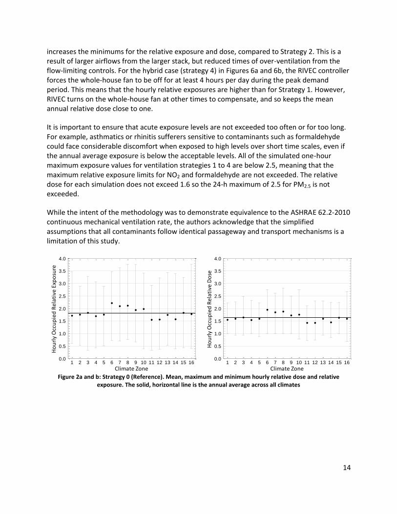
To show compliance with ASHRAE Standard 62.2-2010 the hourly relative dose and exposure was tracked during occupied times and then averaged over the year. The reference case (strategy 0) shown in Figures 2a and 2b has high relative exposures and relative doses, with annual averages for both above 1.5. Hourly maximums for relative exposure reach more than 3.5. Hourly maximums for relative dose exceed 2.5. This result demonstrates the need for ventilation, even though, at 5.2 ACH50, the home is not particularly tight compared to the 3 ACH50 of the International Energy Conservation Code (IECC 2012). Adding mechanical ventilation (strategy 1), in Figures 3a and 3b, brings the averages for relative exposure and dose down to approximately one. The maximums are restricted to 1.5 for relative exposure and 1.25 for relative dose.

The passive stack ventilation (strategy 2), in Figures 4a and 4b, brings the annual mean relative exposure and dose down further, but the maximums increase because of the times of the year when the natural driving forces are low, and the ventilation rate is low. Oversizing and flow-limiting the passive stacks (strategy 3), in Figures 5a and 5b, reduces the maximums and

14

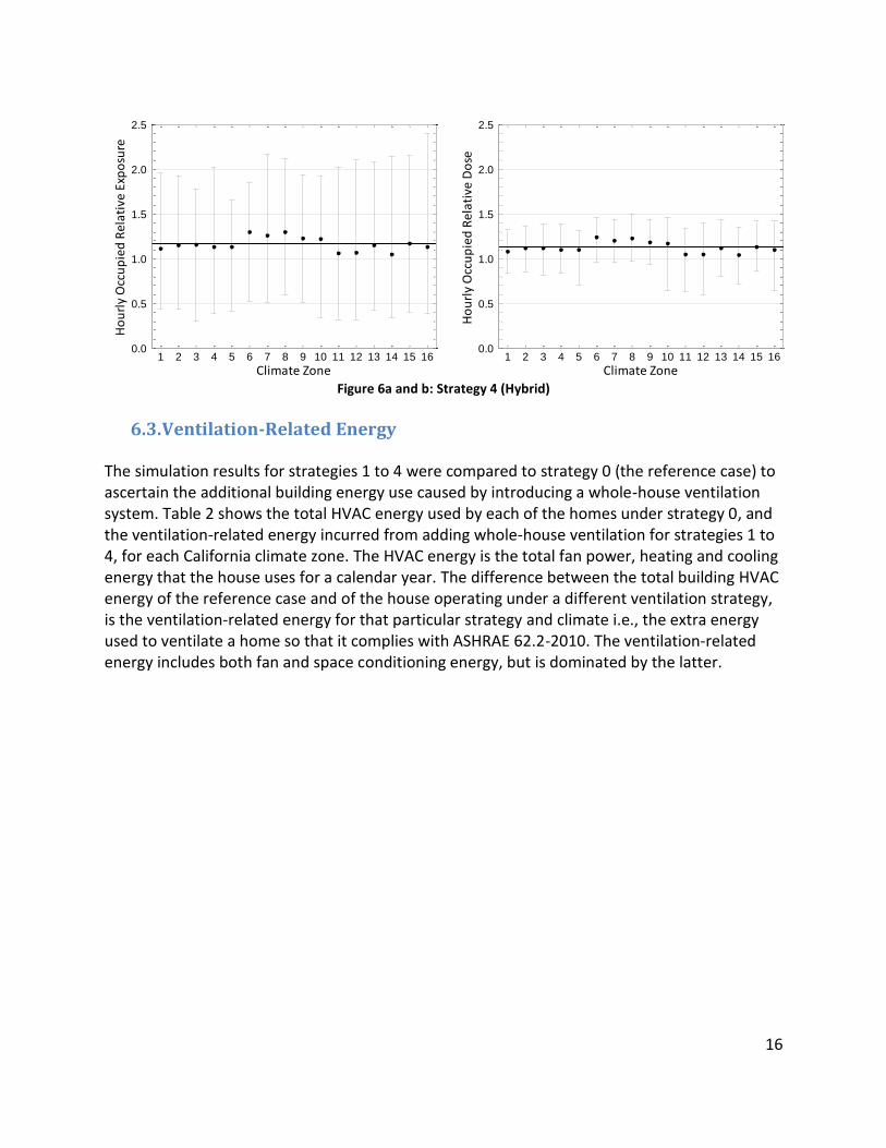
increases the minimums for the relative exposure and dose, compared to Strategy 2. This is a result of larger airflows from the larger stack, but reduced times of over-ventilation from the flow-limiting controls. For the hybrid case (strategy 4) in Figures 6a and 6b, the RIVEC controller forces the whole-house fan to be off for at least 4 hours per day during the peak demand period. This means that the hourly relative exposures are higher than for Strategy 1. However, RIVEC turns on the whole-house fan at other times to compensate, and so keeps the mean annual relative dose close to one.

It is important to ensure that acute exposure levels are not exceeded too often or for too long. For example, asthmatics or rhinitis sufferers sensitive to contaminants such as formaldehyde could face considerable discomfort when exposed to high levels over short time scales, even if the annual average exposure is below the acceptable levels. All of the simulated one-hour maximum exposure values for ventilation strategies 1 to 4 are below 2.5, meaning that the maximum relative exposure limits for NO2 and formaldehyde are not exceeded. The relative dose for each simulation does not exceed 1.6 so the 24-h maximum of 2.5 for PM2.5 is not exceeded.

While the intent of the methodology was to demonstrate equivalence to the ASHRAE 62.2-2010 continuous mechanical ventilation rate, the authors acknowledge that the simplified assumptions that all contaminants follow identical passageway and transport mechanisms is a limitation of this study.

Figure 2a and b: Strategy 0 (Reference). Mean, maximum and minimum hourly relative dose and relative

exposure. The solid, horizontal line is the annual average across all climates

1 2 3 4 5 6 7 8 9 10 11 12 13 14 15 160.0

0.5

1.0

1.5

2.0

2.5

3.0

3.5

4.0

Climate Zone

Ho

url

y O

ccu

pie

d R

elat

ive

Exp

osu

re

1 2 3 4 5 6 7 8 9 10 11 12 13 14 15 160.0

0.5

1.0

1.5

2.0

2.5

3.0

3.5

4.0

Climate Zone

Ho

url

y O

ccu

pie

d R

elat

ive

Do

se

15

Figure 3a and b: Strategy 1 (Mechanical). Note the change in scale on the y-axis

Figure 4a and b: Strategy 2 (Passive-1)

Figure 5a and b: Strategy 3 (Passive-2)

1 2 3 4 5 6 7 8 9 10 11 12 13 14 15 160.0

0.5

1.0

1.5

2.0

2.5

Climate Zone

Ho

url

y O

ccu

pie

d R

elat

ive

Exp

osu

re

1 2 3 4 5 6 7 8 9 10 11 12 13 14 15 160.0

0.5

1.0

1.5

2.0

2.5

Climate Zone

Ho

url

y O

ccu

pie

d R

elat

ive

Do

se

1 2 3 4 5 6 7 8 9 10 11 12 13 14 15 160.0

0.5

1.0

1.5

2.0

2.5

Climate Zone

Ho

url

y O

ccu

pie

d R

elat

ive

Exp

osu

re

1 2 3 4 5 6 7 8 9 10 11 12 13 14 15 160.0

0.5

1.0

1.5

2.0

2.5

Climate Zone

Ho

url

y O

ccu

pie

d R

elat

ive

Do

se

1 2 3 4 5 6 7 8 9 10 11 12 13 14 15 160.0

0.5

1.0

1.5

2.0

2.5

Climate Zone

Ho

url

y O

ccu

pie

d R

elat

ive

Exp

osu

re

1 2 3 4 5 6 7 8 9 10 11 12 13 14 15 160.0

0.5

1.0

1.5

2.0

2.5

Climate Zone

Ho

url

y O

ccu

pie

d R

elat

ive

Do

se

16

Figure 6a and b: Strategy 4 (Hybrid)

6.3. Ventilation-Related Energy

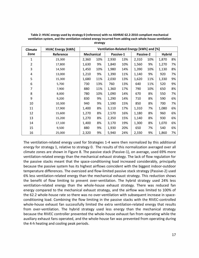
The simulation results for strategies 1 to 4 were compared to strategy 0 (the reference case) to ascertain the additional building energy use caused by introducing a whole-house ventilation system. Table 2 shows the total HVAC energy used by each of the homes under strategy 0, and the ventilation-related energy incurred from adding whole-house ventilation for strategies 1 to 4, for each California climate zone. The HVAC energy is the total fan power, heating and cooling energy that the house uses for a calendar year. The difference between the total building HVAC energy of the reference case and of the house operating under a different ventilation strategy, is the ventilation-related energy for that particular strategy and climate i.e., the extra energy used to ventilate a home so that it complies with ASHRAE 62.2-2010. The ventilation-related energy includes both fan and space conditioning energy, but is dominated by the latter.

1 2 3 4 5 6 7 8 9 10 11 12 13 14 15 160.0

0.5

1.0

1.5

2.0

2.5

Climate Zone

Ho

url

y O

ccu

pie

d R

elat

ive

Exp

osu

re

1 2 3 4 5 6 7 8 9 10 11 12 13 14 15 160.0

0.5

1.0

1.5

2.0

2.5

Climate Zone

Ho

url

y O

ccu

pie

d R

elat

ive

Do

se

17

Table 2: HVAC energy used by strategy 0 (reference) with no ASHRAE 62.2-2010 compliant mechanical ventilation system, and the ventilation-related energy incurred from adding each whole-house ventilation

strategy

Climate Zone

HVAC Energy [kWh] Ventilation-Related Energy [kWh] and [%]

Reference Mechanical Passive-1 Passive-2 Hybrid

1 23,300 2,360 10% 2,930 13% 2,310 10% 1,870 8% 2 17,800 1,630 9% 1,840 10% 1,560 9% 1,270 7% 3 14,500 1,450 10% 1,980 14% 1,390 10% 1,130 8%

4 13,000 1,210 9% 1,390 11% 1,140 9% 920 7% 5 15,300 1,680 11% 2,030 13% 1,620 11% 1,330 9% 6 5,700 730 13% 760 13% 640 11% 520 9% 7 7,900 880 11% 1,360 17% 790 10% 650 8% 8 8,000 780 10% 1,090 14% 670 8% 550 7% 9 9,200 830 9% 1,290 14% 710 8% 590 6%

10 10,300 940 9% 1,590 15% 850 8% 700 7% 11 17,900 1,400 8% 3,110 17% 1,310 7% 1,080 6% 12 15,600 1,270 8% 2,570 16% 1,180 8% 960 6% 13 15,200 1,270 8% 2,350 15% 1,140 8% 930 6%

14 17,100 1,400 8% 3,170 19% 1,300 8% 1,070 6% 15 9,500 880 9% 1,930 20% 650 7% 540 6% 16 25,000 2,320 9% 5,940 24% 2,330 9% 1,860 7%

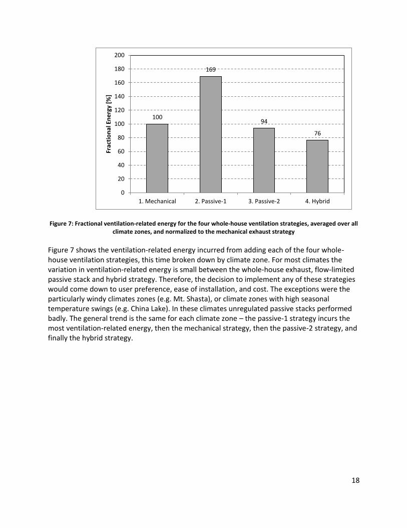
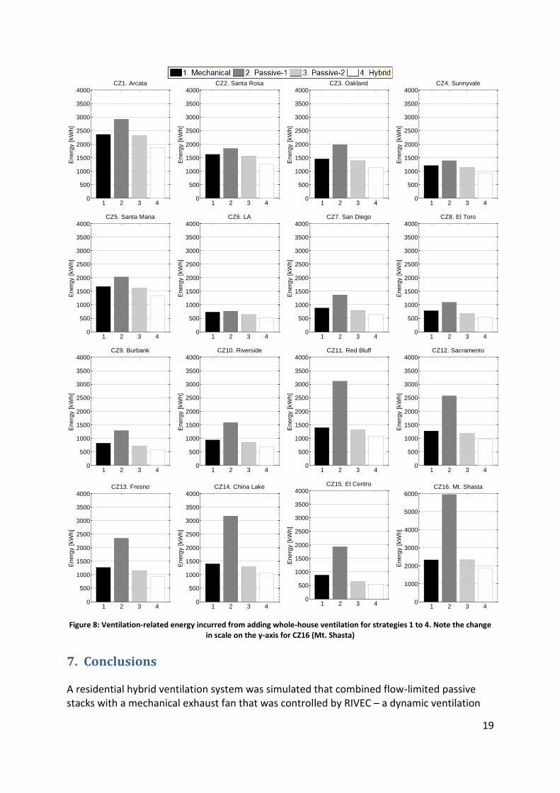
The ventilation-related energy used for Strategies 1-4 were then normalized by this additional energy for strategy 1, relative to strategy 0. The results of this normalization averaged over all climate zones are shown in Figure 8. The passive stack (Passive-1), on average, used 69% more ventilation-related energy than the mechanical exhaust strategy. The lack of flow regulation for the passive stacks meant that the space-conditioning load increased considerably, principally because the passive system has its highest airflows coincident with the biggest indoor-outdoor temperature differences. The oversized and flow-limited passive stack strategy (Passive-2) used 6% less ventilation-related energy than the mechanical exhaust strategy. This reduction shows the benefit of flow limiting to prevent over-ventilation. The hybrid strategy used 24% less ventilation-related energy than the whole-house exhaust strategy. There was reduced fan energy compared to the mechanical exhaust strategy, and the airflow was limited to 100% of the 62.2 whole-house rate so there was no over-ventilation with subsequent increase in space-conditioning load. Combining the flow limiting in the passive stacks with the RIVEC-controlled whole-house exhaust fan successfully limited the extra ventilation-related energy that results from over-ventilation. The hybrid strategy used less energy than the mechanical strategy because the RIVEC controller prevented the whole-house exhaust fan from operating while the auxiliary exhaust fans operated, and the whole-house fan was prevented from operating during the 4-h heating and cooling peak periods.

18

Figure 7: Fractional ventilation-related energy for the four whole-house ventilation strategies, averaged over all climate zones, and normalized to the mechanical exhaust strategy

Figure 7 shows the ventilation-related energy incurred from adding each of the four whole-house ventilation strategies, this time broken down by climate zone. For most climates the variation in ventilation-related energy is small between the whole-house exhaust, flow-limited passive stack and hybrid strategy. Therefore, the decision to implement any of these strategies would come down to user preference, ease of installation, and cost. The exceptions were the particularly windy climates zones (e.g. Mt. Shasta), or climate zones with high seasonal temperature swings (e.g. China Lake). In these climates unregulated passive stacks performed badly. The general trend is the same for each climate zone – the passive-1 strategy incurs the most ventilation-related energy, then the mechanical strategy, then the passive-2 strategy, and finally the hybrid strategy.

100

169

94

76

0

20

40

60

80

100

120

140

160

180

200

1. Mechanical 2. Passive-1 3. Passive-2 4. Hybrid

Frac

tio

nal

En

erg

y [%

]

19

Figure 8: Ventilation-related energy incurred from adding whole-house ventilation for strategies 1 to 4. Note the change

in scale on the y-axis for CZ16 (Mt. Shasta)

7. Conclusions

A residential hybrid ventilation system was simulated that combined flow-limited passive stacks with a mechanical exhaust fan that was controlled by RIVEC – a dynamic ventilation

1 2 3 40

500

1000

1500

2000

2500

3000

3500

4000CZ1. Arcata

En

erg

y [

kW

h]

1 2 3 40

500

1000

1500

2000

2500

3000

3500

4000CZ2. Santa Rosa

Energ

y [

kW

h]

1 2 3 40

500

1000

1500

2000

2500

3000

3500

4000CZ3. Oakland

En

erg

y [

kW

h]

1 2 3 40

500

1000

1500

2000

2500

3000

3500

4000CZ4. Sunnyvale

En

erg

y [

kW

h]

1 2 3 40

500

1000

1500

2000

2500

3000

3500

4000CZ5. Santa Maria

En

erg

y [

kW

h]

1 2 3 40

500

1000

1500

2000

2500

3000

3500

4000CZ6. LA

En

erg

y [

kW

h]

1 2 3 40

500

1000

1500

2000

2500

3000

3500

4000CZ7. San Diego

Energ

y [

kW

h]

1 2 3 40

500

1000

1500

2000

2500

3000

3500

4000CZ8. El Toro

En

erg

y [

kW

h]

1 2 3 40

500

1000

1500

2000

2500

3000

3500

4000CZ9. Burbank

En

erg

y [

kW

h]

1 2 3 40

500

1000

1500

2000

2500

3000

3500

4000CZ10. Riverside

En

erg

y [

kW

h]

1 2 3 40

500

1000

1500

2000

2500

3000

3500

4000CZ11. Red Bluff

En

erg

y [

kW

h]

1 2 3 40

500

1000

1500

2000

2500

3000

3500

4000CZ12. Sacramento

Energ

y [

kW

h]

1 2 3 40

500

1000

1500

2000

2500

3000

3500

4000CZ13. Fresno

En

erg

y [

kW

h]

1 2 3 40

500

1000

1500

2000

2500

3000

3500

4000CZ14. China Lake

En

erg

y [

kW

h]

1 2 3 40

500

1000

1500

2000

2500

3000

3500

4000CZ15. El Centro

En

erg

y [

kW

h]

1 2 3 40

1000

2000

3000

4000

5000

6000CZ16. Mt. Shasta

En

erg

y [

kW

h]

20

controller. For comparison, two purely passive systems, a purely mechanical system, and a naturally ventilated (infiltration only) reference house were also simulated. The simulation results show that the hybrid system can provide equivalent IAQ to mechanical and passive systems for less expenditure of energy. The passive and hybrid systems provide equivalent (or better) exposure to pollutants compared to a continuously operating mechanical ventilation system that meets ASHRAE 62.2-2010. The passive and hybrid systems also meet hourly standards of acute exposure for key indoor household pollutants. The naturally ventilated reference house did not meet acute exposure limits for PM2.5 and had a chronic relative dose approximately 50% higher than the ASHRAE 62.2-2010 compliant home. Averaged over 16 California climate zones, the hybrid system used 24% less energy than a continuously-operating whole-house exhaust fan.

Passive and hybrid ventilation systems need to be sized appropriately to limit times of over- and under-ventilation. Three passive/hybrid approaches were examined. The first passive approach sized the passive stacks so that the airflow through the stacks met or exceeded ASHRAE 62.2-2010 for at least 80% of the year. Because this sizing approach provided equivalent IAQ compared to a continuously operating ASHRAE 62.2-2010 compliant mechanical ventilation system, the sizing guidance developed in this study is optimum for IAQ purposes. However, on average this sizing method resulted in 70% more ventilation-related energy use than a mechanical system due to over-ventilating in extreme weather. The second passive approach of oversizing and flow limiting the passive stacks to 125% of the ASHRAE 62.2-2010 continuous mechanical ventilation flow rate, provided approximately 75% ventilation-related energy savings over uncontrolled passive stacks (or approximately 5% savings compared to mechanical ventilation). The hybrid system used the oversized stacks limited to 100% of the ASHRAE 62.2-2010 continuous mechanical ventilation flow rate, and provided a 25% reduction in energy requirements compared to the mechanical system. The results of this study indicate that these are appropriate sizing strategies for passive and hybrid systems.

21

8. References

ACCA 2006. Manual J Residential Load Calculation 8th Edition, Washinton D.C., Air Conditioning Contractors of America.

ASHRAE 2009a. ASHRAE Handbook. Fundamentals, Atlanta, Ga., American Society of Heating, Refrigerating, and Air-Conditioning Engineers.

ASHRAE 2009b. Standard 160P: Design Criteria for Moisture Control in Buildings. Atlanta, GA: American Society of Heating, Refrigeration and Air Conditioning Engineers.

ASHRAE 2010. Standard 62.2: Ventilation and Acceptable Indoor Air Quality in Low-Rise Residential Buildings. Atlanta, GA: American Society of Heating, Refrigeration and Air Conditioning Engineers.

AXLEY, J. W. 2001. Residential Passive Ventilation: Evaluation and Design. AIVC Technical Note 54. Air Infiltration and Ventilation Centre.

CEC 2008a. Alternative Calculation Method (ACM) approval manual for the 2008 Energy Efficiency Standards for nonresidential buildings. Sacramento, Calif.: California Energy Commission,.

CEC 2008b. Title 24, Part 6, California Code of Regulations: California's Energy Efficiency Standards for Residential and Nonresidential Buildings. Part 6. California Energy Commission.

CHAN, W. R., NAZAROFF, W. W., PRICE, P. N., SOHN, M. D. & GADGIL, A. J. 2005. Analyzing a database of residential air leakage in the United States. Atmospheric Environment, 39, 3445-3455.

DOLS, W. S., EMMERICH, S. J. & POLIDORO, B. J. 2012. NIST Technical Note 1735 LoopDA 3.0 - Natural Ventilation Design and Analysis Software User Guide. NIST.

ELGER, D. F., WILLIAMS, B. C., CROWE, C. T. & ROBERSON, J. A. 2012. Engineering Fluid Mechanics, Wiley.

EMMERICH, S. J., HOWARD-REED, C. & GUPTE, A. 2005. Modeling the IAQ Impact of HHI Interventions in Inner-city Housing. National Institute of Standards and Technology.

FOREST, T. W. & WALKER, I. S. Attic Ventilation Model. ASHRAE/DOE/BTECC 5th Conf. on Thermal Performance of Exterior Envelopes of Buildings, 1992. ASHRAE, 399-408.

FOREST, T. W. & WALKER, I. S. 1993a. Attic Ventilation and Moisture. Canada Mortgage and Housing Corporation.

FOREST, T. W. & WALKER, I. S. Moisture Dynamics in Residential Attics. CANCAM, 1993b Queens University, Kingston, Ontario, Canada.

HAYSOM, J. C. & SWINTON, M. C. 1987. The influence of termination configuration on the flow performance of flues, Canada Mortgage and Housing Corporation.

HEISELBERG, P., DELSANTE, A. & VIK, T. A. 2001. Hybrid Ventilation - State-of-the-Art Review. Annex35 HybVent, IEA, 20.

22

MANSSON, L.-G. 1995. Evaluation and Demonstration of Domestic Ventilation Systems - State of the Art. Energy Conservation in Buildings and Community Systems Program. Stockholm: IEA.

MORTENSEN, D. K., SHERMAN, M. H. & WALKER, I. S. Energy and Air Quality Implications of Passive Ventilation in Residential Buildings. ACEEE Summer Study, 2010 Washington D.C.: American Council for an Energy Efficient Economy.

NITTLER, K. & WILCOX, B. 2008. Residential Housing Starts and Prototypes. California Building Energy Efficiency Standards.

OFFERMANN, F. J. 2009. Ventilation and Indoor Air Quality in New Homes. PIER Collaborative Report. California Energy Commission & California Environmental Protection Agency Air Resources Board.

SHERMAN, M. H. 2006. Efficacy of Intermittent Ventilation for Providing Acceptable Indoor Air Quality. ASHRAE Transactions, 111, 93-101.

SHERMAN, M. H., LOGUE, J. M. & SINGER, B. C. 2011. Infiltration effects on residential pollutant concentrations for continuous and intermittent mechanical ventilation approaches. Hvac&R Research, 17, 159-173.

SHERMAN, M. H. & MATSON, N. E. 1997. Residential Ventilation and Energy Characteristics. ASHRAE Transactions, 103.

SHERMAN, M. H. & WALKER, I. S. 2008. Energy Impact of Residential Ventilation Standards in California. ASHRAE Transactions, 114, 482-493.

SHERMAN, M. H. & WALKER, I. S. 2011. Meeting residential ventilation standards through dynamic control of ventilation systems. Energy and Buildings, 43, 1904-1912.

SHERMAN, M. H., WALKER, I. S. & DICKERHOFF, D. J. 2009. EISG Final Report: Residential Integrated Ventilation Controller. Energy Innovations Small Grant #55044A. California Energy Commission Public Interest Energy Research.

SHERMAN, M. H. & WILSON, D. J. 1986. Relating Actual and Effective Ventilation in Determining Indoor Air-Quality. Building and Environment, 21, 135-144.

SHERMAN, M. H., WALKER, I. S. & LOGUE, J. M. 2012. Equivalence in Ventilation and Indoor Air Quality. HVAC&R Research 18(4), 760-773

SIEGEL, J. A. 1999. The REGCAP Simulation: Predicting Performance in New California Homes. MSc, University of California, Berkeley.

SIEGEL, J. A., WALKER, I. S. & SHERMAN, M. H. Delivering Tons to the Register: Energy Efficient Design and Operation of Residential Cooling Systems. ACEEE Summer Study, 2000 Washington, DC. American Council for an Energy Efficient Economy, 295-306.

STEPHEN, R. K., PARKINS, L. M. & WOOLLISCROFT, M. 1994. Passive stack ventilation systems: design and installation. BRE Information Paper. Building Research Centre.

23

SUNDELL, J., LEVIN, H., NAZAROFF, W. W., CAIN, W. S., FISK, W. J., GRIMSRUD, D. T., GYNTELBERG, F., LI, Y., PERSILY, A. K., PICKERING, A. C., SAMET, J. M., SPENGLER, J. D., TAYLOR, S. T. & WESCHLER, C. J. 2011. Ventilation rates and health: multidisciplinary review of the scientific literature. Indoor Air, 21, 191-204.

SUTCLIFFE, G. L. 1899. The Principles and Practice of Modern House-Construction, London, Blackie and Son Ltd.

TURNER, W. J. N. & WALKER, I. S. 2012 Advance controls and sustainable systems for residential ventilation. Lawrence Berkeley National Laboratory, Berkeley, CA, LBNL-5968E

VAN HEEMST, L. V. 2001. Hybrid Ventilation: An Intergral Solution for Ventilation, Health and Energy, Annex35 HybVent, IEA, TU-Delft.

WALKER, I. S. 1989. Single Zone Air Infiltration Modelling. University of Alberta, Edmonton.

WALKER, I. S. 1993. Attic Ventilation, Heat and Moisture Transfer. PhD, University of Alberta.

WALKER, I. S., DEGENETAIS, G. & SIEGEL, J. A. 2002. Simulations of Sizing and Comfort Improvements for Residential Forced air heating and Cooling Systems. Berkeley, California: Lawrence Berkeley National Laboratory, LBNL-47309.

WALKER, I. S., FOREST, T. W. & WILSON, D. J. 2006. An attic-interior infiltration and interzone transport model of a house. Building and Environment, 40, 701-718.

WALKER, I. S. & SHERMAN, M. H. 2008. Energy Implications of Meeting ASHRAE 62.2. ASHRAE Transactions, 114, 505-516.

WALKER, I. S., SHERMAN, M. H. & SIEGEL, J. A. 1999. Distribution Effectiveness and Impacts on Equipment Sizing. CIEE Contract Report. Berkeley, California: Lawrence Berkeley National Laboratory, LBNL-43724.

WALKER, I. S., SIEGEL, J. & DEGENETAIS, G. 2001. Simulation of Residential HVAC System Performance. ESIM Conference. CANMET Energy Technology Centre/Natural Resources Canada, Ottawa, Ontario, Canada.

WILCOX, S. & MARION, W. 2008. User's Manual for TMY3 Data Sets. In: NREL/TP-581-43156 (ed.). Golden, Colorado: National Renewable Energy Laboratory.

WILSON, D. J. & WALKER, I. S. Feasibility of Passive Ventilation by Constant Area Vents to Maintain Indoor Air Quality in Houses. Indoor Air Quality, 1992a San Francisco.

WILSON, D. J. & WALKER, I. S. 1992b. Passive Ventilation to Maintain Indoor Air Quality. Alberta, Canada: University Of Alberta, Department of Mechanical Engineering.