wider research paper 2007/10 the determinants of … · (ols, tobit, re-tobit) and allowances for...

Copyright © UNU-WIDER 2007 1North-West University, Potchefstroom; 2UNU-WIDER, Helsinki. This study has been prepared within the UNU-WIDER project on New Directions in Development Economics directed by Augustin Fosu. UNU-WIDER acknowledges the financial contributions to the research programme by the governments of Denmark (Royal Ministry of Foreign Affairs), Finland (Ministry for Foreign Affairs), Norway (Royal Ministry of Foreign Affairs), Sweden (Swedish International Development Cooperation Agency—Sida) and the United Kingdom (Department for International Development). ISSN 1810-2611 ISBN 92-9190-949-1 ISBN 13 978-92-9190-949-0

Research Paper No. 2007/10 The Determinants of Regional Manufactured Exports from a Developing Country Marianne Matthee1 and Wim Naudé2 February 2007

Abstract

In this paper, the question of the location of exporters of manufactured goods within a country is investigated. Based on insights from new trade theory, the new economic geography (NEG) and gravity-equation modelling, an empirical model is specified with agglomeration and increasing returns (the home market effect) and transport costs (proxied by distance) as major determinants of the location decision of exporters. Data from 354 magisterial districts in South Africa are used with a variety of estimators (OLS, Tobit, RE-Tobit) and allowances for data shortcomings (bootstrapped standard errors and analytical weights) to identify the determinants of regional manufactured exports. It is found that the home-market effect (measured by the size of local GDP) and distance (measured as the distance in km to the nearest port) are significant determinants of regional manufactured exports. This paper contributes to the literature by using developing country data, and by adding to the small literature on this topic. This paper complements recent work on the determinants of exports from European regions and finds that the home market effect is relatively more important in the developing country context (South Africa), a finding consistent with theoretical NEG model. Keywords: South Africa, manufactured exports, home market effect, domestic transport costs JEL classification : R12, R49, F12, F14

The World Institute for Development Economics Research (WIDER) was established by the United Nations University (UNU) as its first research and training centre and started work in Helsinki, Finland in 1985. The Institute undertakes applied research and policy analysis on structural changes affecting the developing and transitional economies, provides a forum for the advocacy of policies leading to robust, equitable and environmentally sustainable growth, and promotes capacity strengthening and training in the field of economic and social policy making. Work is carried out by staff researchers and visiting scholars in Helsinki and through networks of collaborating scholars and institutions around the world. www.wider.unu.edu [email protected]

UNU World Institute for Development Economics Research (UNU-WIDER) Katajanokanlaituri 6 B, 00160 Helsinki, Finland Typescript prepared by Lorraine Telfer-Taivainen at UNU-WIDER The views expressed in this publication are those of the author(s). Publication does not imply endorsement by the Institute or the United Nations University, nor by the programme/project sponsors, of any of the views expressed.

Acknowledgements

We are grateful to Augustin Fosu, Waldo Krugell and Thomas Gries for helpful comments on an earlier draft. The usual disclaimer applies.

1

1 Introduction

Theoretical and empirical work in international trade has, with a few exceptions, predominantly focused on trade between countries, as opposed to focusing on where exports originate within a country. International trade theory until fairly recently assumed away all elements that might make consideration of the geography of exports possible. For instance, transport costs, distance, market size, scale economies and agglomeration were only recently incorporated into trade models. In this respect, important initial contributions on the integration of regional science and international trade theory were made by Krugman (1979, 1980, 1991), Venables (2001), Fujita et al. (2001: 367) and Fujita and Krugman (2004). Despite these advances, relatively little evidence have been forthcoming as to the appropriateness of these theoretical models (Brakman et al. 2001; Naudé and Krugell 2006; Venables 2005; Gries and Naudé 2007). Moreover, where transport costs in international trade are concerned, empirical work has so far tended to focus on international shipping costs (Clark et al. 2004; Hummels 1999; Radelet and Sachs 1998). This paper’s contribution is to present empirical evidence on the geographical location and determinants of exports from a developing country. Understanding these determinants may be important given the wide consensus that exists on the positive impact of export growth on economic growth and development (see Fosu 1990a, 1990b; and more recently Foster 2006; Hausman et al. 2006) and on the potential for differential export performance to contribute to spatial inequality (see Kanbur and Venables 2005). Existing studies on this topic focus only on developed countries (for example Nicolini 2003). A developing country perspective is given in this paper using data from South Africa’s 354 magisterial districts. The focal point is manufactured exports, as manufacturing firms tend to be more footloose than for example firms in mining or agriculture. It is found that local demand (or economic growth) positively influences exports, whereas distance from a port decreases exports. The further exporters are located from an export hub (such as a port), the less their manufactured exports. Distance (i.e. domestic transport costs) therefore matters. The paper continues in Section 2 by describing the modelling approach from the framework of theoretical contributions on the topic. Thereafter in Section 3 the data and estimators used are discussed. Before the results are discussed in Section 5, the profile and patterns of manufactured exports in South Africa are described in Section 4. The paper concludes with a summary and suggestions for further research in Section 6.

2 Modelling approach

2.1 Theoretical background

In traditional explanations of trade (such as the Heckscher-Ohlin model) patterns of trade between countries depend on natural resources, skills and factors of production. It is assumed that trade takes place in a perfectly competitive and frictionless (pinpoint) world without transport costs (Salvatore 1998: 766).

2

Only relatively recently, in the new trade theories, has the role of transport costs as a determinant of trade in international trade been recognised (see e.g. initial contributions by Krugman 1979, 1980). Herein, Samuelson’s (1952) concept of ‘iceberg’ transport costs is frequently used. With iceberg transport costs, goods can be shipped freely, but only a fraction of goods (g) arrive at the relevant destination, with (1 – g) being lost in transit (i.e. it melts away). The fraction lost in transit is seen as the transport cost incurred (Krugman 1980; Fujita and Krugman 2004). According to Fujita and Krugman (2004), using iceberg transport costs has two advantages. First, it eliminates the need to analyse the transport sector as another industry. Second, it simplifies the description of how monopolistic firms set their prices (i.e. it erases the incentive to absorb transport costs, charging a lower FOB price for exports than for domestic sales). Krugman (1991) redefined the ‘iceberg’ cost function as an explicit geographical distance-related function (McCann 2005). Both international and domestic transport costs can be distinguished, and have significant effects on trade. As far as international transport costs are concerned, Radelet and Sachs (1998) analyse the impact of international transport costs on the international competitiveness of developing countries. They find that transport costs are influenced by geographical factors such as distance to markets and access to ports, which in turn have an effect on manufactured exports and long-term economic growth. Countries with lower transport costs have experienced more rapid growth in manufactured exports as well as in overall economic growth during the past three decades, than countries with higher transport costs. High transport costs elevate the cost of producing manufactures by increasing the price of imported intermediate and capital goods. These elevated production costs, together with high transport costs, impede the price competitiveness of manufactured exports (Radelet and Sachs 1998; Hoffmann 2002). Limão and Venables (2001) find that landlocked developing countries tend to have higher transport costs (approximately 50 per cent) and lower trade volumes (around 60 per cent) than coastal countries. Clark et al. (2004: 417) find that transport costs are a significant determinant of bilateral trade between Latin America and the USA, and that port efficiency is an important determinant of international shipping costs (improving port efficiency from the 25th to the 75th percentile can reduce shipping costs by up to 12 per cent). As far as domestic transport costs and the relationship between transport costs and firm location are concerned, the so-called ‘home market’ effect has been offered to explain the observed spatial concentration of industries. Krugman (1980) explains that if manufacturing firms experience increasing returns to scale in the face of positive transport costs, they will locate in the vicinity of the largest market. This implies that one can expect the concentration of production to enable increasing returns to scale, while locating near the largest market minimises transport costs. As a determinant of regional manufacturing exports the home market effect implies that manufacturing firms will export those products for which there is a large domestic (local) demand (Armstrong and Taylor 2000: 437). Transport costs are the determining factor for the home market effect. By locating near the larger market, firms are able to achieve increasing returns to scale and at the same time minimise their transport costs. This increases the real wage of workers in that region and makes it a more attractive place to live (Brakman et al. 2001). According to Brakman et al. (2001), transport costs are the main identifying characteristic of regions in the core-periphery model of the new economic geography (NEG) theory. In the

3

model, transport costs are assumed zero within a region and positive between two regions. Transport costs consist of various elements that hamper trade such as tariffs, language, cultural barriers as well as the actual costs incurred in moving goods from one place to another (Krugman 1991; Brakman et al. 2001; Fujita et al. 2001). If transport costs were high, trade would not take place, as it would be too costly—exports and imports are so expensive that only home production is possible. Production will be spread out to be close to demand. If transport costs were low, there would also be no trade or agglomeration since the two regions would be ex ante identical and neither would have the forces, such as a thick labour market or inter-industry linkages, which create the propensity for agglomeration. Thus, it is in an intermediate range that transport costs matter for trade and agglomeration. Below this threshold level of transport costs, manufacturers choose the location with large local demand. Local demand will be large precisely where the majority of manufacturers choose to locate. The result is agglomeration at the core and trade with the periphery (Krugman 1991; Brakman et al. 2001; Fujita et al. 2001). From the above, the main determinants of exports from a specific location are distance (transport costs) and the home market effect. Empirical evidence support these conclusions (Venables 2001; see also Crafts and Mulatu 2005 for a discussion of the location of industry in Britain). For instance, countries tend to trade with proximate partners (Grossman, cited in The Round Table 2004), even if transport costs over distance have fallen (Hummels 1999). Approximately half of the world’s trade takes place between countries located within 3,000 km of each other (The Round Table 2004). The distance of trade for the average countries in the world has decreased, implying that distance matters (Carrere and Schiff 2004). A possible reason for this occurrence is that distance is costly. It directly increases transaction costs in terms of additional transport costs of shipping goods, time costs of shipping date-sensitive goods, the costs of contracting at a distance (search costs), costs of obtaining information on remote economies and costs of communicating with distant locations (Overman et al. 2001; Venables 2001). Redding and Schott (2003: 516) also show that firms that are located at some distance from final markets face transport costs on both their sales as well as on their inputs, and as a consequence will have less value added available to remunerate labour, which in turn will reduce incentives for investment in human capital. This is an additional channel through which distance from markets can reduce a region’s growth and explain spatial economic inequality.

2.2 Regional trade model

In the previous section trade, as a result of agglomeration, was explained. Various other models (for example the gravity model of trade and the price elasticity model of supply and demand) have been developed to explain trade and more specifically, the determinants of the exports of countries. What distinguishes the gravity model of trade from other models is that it incorporates a spatial element, namely distance, to the explanation of trade. As indicated, space in the form of distance, is highly relevant as one of the determinants of trade in the NEG theory. The gravity model states that bilateral trade flows between countries are determined by their respective incomes, the distance between them and other country-specific factors such as language, geographical continuity, trade agreements and colonial ties (Deardorff 1995; Head 2003). The general conclusion from the existing empirical studies is that the further the

4

countries are located from one another, the lower are the trade flows due to increasing transport costs (Brakman et al. 2001; Nicolini 2003). The gravity model is however, not without shortcomings and has been widely criticised for not having a solid theoretical foundation. The theoretical foundation underlying this model has been the subject of research for more than three decades (Anderson 1979; Bergstrand 1985, 1989, 1990; Deardorff 1995; Evenett and Keller 1998). Deardorff (1995) shows that the gravity equation can be derived from any of the trade theories, as it characterises many of their attributes. Indeed, the gravity equation has also been derived from the new trade theory. For example, Feenstra et al. (2001) employ the gravity equation in conditions of monopolistic competition to test for the home market effect. They use the incomes of the country pairs as proxies for the home market effect and find that it exist for differentiated but not for homogeneous goods (domestic income elasticity exceeds the partner income elasticity). Therefore, with subtle differences in the parameter values, Feenstra et al. (2001) found that the gravity equation is supportive of an increasing returns model as embodied in new trade theory. It is only in the work of Nicolini (2003) that the focus is no longer on countries but on the regions within countries. Up to this point, no other study has engaged in such an approach. Nicolini (2003) adapts the gravity model to develop and test a theoretical model (based on NEG theory) of the determinants of singular (export) flows from regions. Her study finds that factors that determine a country’s exports differ from the factors that determine where those exports originate within a country. Nicolini’s (2003) theoretical framework assumes (a) a utility function of consumers that consume both local and imported goods and (b) a production function of local and foreign firms. Exporting the goods incurs transport costs (in the form of iceberg transport costs). As her model only considers singular trade flows, she derives the home market effect from the assumption that the demand for local goods exceeds that of imported goods. The reasoning behind this assumption is as follows: when local firms agglomerate due to the effect of circular causation, they are able to specialise and achieve increasing returns to scale. This lowers their production costs and subsequently prices. Consumers demand local firms’ goods as they are cheaper than imported goods. As demand increases, firms are able to expand and eventually export their goods. Export is therefore the result of increased demand that originates from circular causation (i.e. the home market effect). In the following section, Nicolini’s (2003) empirical model is tested with developing country data (from South Africa) in order to compare and contrast results between developed and developing country regions. Whilst Nicolini’s (2003) empirical models is tested for a developing country, more sophisticated estimators are used since not all regions within a developing country export, in contrast to Nicolini’s developed country sample where all regions had positive exports.

3 Empirical model

3.1 Estimating equation

The estimating equation follows that of Nicolini (2003) and implies that exports (EXPR) from a region are determined by a geographical component (GeoR) particular to each

5

region, the home market effect (HMR) of each region and specific regional features (SER). The equation as developed by Nicolini (2003) is:

)()()()( 321 RRRR SELogHMLogGeoLogcEXPLog βββ +++= (1) Nicolini (2003) measures the home market effect by using the GDP per region corrected by the geographical surface area of the region (GDP per km²) in order to account for the size of the local market. She finds that the home market effect explains the export intensity of the regions. The geographical component captures transport costs. Transport costs are proxied by using two different measures, the surface area of a region (i.e. the geographic area in km²) and the transport intensity (the local transport infrastructure or network) of each region. Nicolini (2003) finds that the surface area of a region affects the density of exports negatively (and concludes that distance matters, also see Section 2.1) and increased transport intensity facilitates trade flows (infrastructure is positively correlated with trade volume, also see Bougheas et al. 1999). She adds dummies in her test for whether or not a region is adjacent to a foreign country. Due to data constraints, the estimating equation for this paper has to be modified slightly, but still follows Nicolini’s (2003) approach. The equation is as follows:

)()()()( 321 MMMM SELogHMLogDistLogcEXPLog βββ +++= (2) The home-market effect (HMM) is captured by the GDP per magisterial district.1 The geographical component (DistM) here is also measured using two proxies, namely the distance from each magisterial district to its nearest export hub (also see Section 4) and the surface area of each magisterial district. The influence of domestic transport costs on regional exports is captured through the implementation of these proxies. The use of dummies for adjacency is not relevant.

3.2 Data

The discussion on the data used in this paper needs to be preceded by a short description of the magisterial districts (which constitute the regions in this paper) in South Africa. South Africa has nine provinces, each with a number of magisterial districts. The Western Cape has 42 magisterial districts, the Eastern Cape 78, the Northern Cape 26, the Free State 52, KwaZulu Natal 51, the North West 19, Gauteng 24, Mpumalanga 31 and the Limpopo province has 31 magisterial districts. The number of magisterial districts total 354 (Global Insight Southern Africa 2006). Each magisterial district is unique in the sense that their sizes, levels of income, numbers of exports, climate conditions and even cultural backgrounds differ (Gries and Naudé 2007). In addition to their different attributes, the districts’ economic development has not been on par since 1994 (Bosker and Krugell 2007). South Africa’s magisterial districts therefore provide valuable insight into why some regions or locations export and others do not.

1 In this section the concept of a ‘region’ corresponds to a magisterial district (an area governed by a

local authority) in the South African case. There are 354 magisterial districts, which formed the basis for the country’s 1996 and 2001 censuses. The 354 magisterial districts are depicted in Figure 1. The 354 magisterial districts, which acted as borders for local authorities, were changed after 2000 to 283 municipal areas. However, for present purposes, it is more useful to use the 354 regions since it provides a finer geographical spread due to the higher number of separate regions.

6

Figure 1 provides a graphical illustration of South Africa’s magisterial districts. The shaded districts are those that have positive manufactured exports. The relative volumes of exports are indicated according to the percentage of exports from a particular district. For instance, the areas shaded black are areas where the district contributes more than 1 per cent of total manufactured exports and the areas shaded grey between 0.1 and 0.99 per cent.

Figure 1: Exports per magisterial district

Source: Authors’ calculations (map drawn by GISCOE).

Panel data on manufactured exports was obtained from Global Insight Southern Africa’s Regional Economic Focus database (Global Insight 2006).This database is compiled from data supplied by the South African Revenue Services and the Department of Customs and Excise. The documentation required from exporters by the Department of Customs and Excise captures their postal codes or street addresses. This data per postal code was mapped to the 354 magisterial districts (the cross-section units) to provide information on each magisterial district. The magisterial allocations were then compared to the national totals contained in the South African Reserve Bank Quarterly Bulletin (Gries and Naudé 2007). Data for exports, GDP per magisterial district was obtained from this database. The Regional Economic Focus Database also provides geographical data of each magisterial district (data on the surface area (in km²) was used as one of the proxies for domestic transport costs). The only other variable, for which data was obtained, is distance. In gravity models, distances from city centre to city centre is calculated. In this paper, actual distances in South Africa between the magisterial districts and the major export hubs are used. The

7

export hubs are: City Deep (a dry port for containers situated in Gauteng), Durban harbour (in KwaZulu-Natal), Port Elizabeth harbour (in the Eastern Cape) and Cape Town harbour (situated in the Western Cape). The reason for including only these ports is that that majority of manufactured exports move through them as they are equipped to handle containers and higher value products. These hubs are also situated on one or more of the three main freight corridors namely Gauteng to Durban, Gauteng to Cape Town and Gauteng to Port Elizabeth. Around 62 per cent of all South Africa’s imports and exports are moved through one or more of these corridors (DoT 2005). In terms of the data, the shortest distance from each magisterial district to one of these hubs was chosen as the distance variable, as it is assumed that exporters strive to minimise their transport costs. The internet service Shell Geostar (www.shellgeostar.co.za) was used to obtain these distances. Shell Geostar is a mapping service that provides detailed maps and distances between any two locations in South Africa. Table 1 provides the list of variables.

Table 1: List of variables

Variable Description

Log Export

Log GDP

Log Distance

Log Surface

Logarithm of magisterial exports (in actual value)

Logarithm of magisterial GDP (in actual value)

Logarithm of distances (in km)

Logarithm of regional surface area (in km2)

Note: In each instance the logarithm of the variables is used as it removes non-linearities, limits changes of the variance of the variables and allows for interpretation of the coefficients as elasticities (Vogelvang 2005: 363).

Source: Authors’ calculations.

3.3 Estimators

In this paper, various estimators are applied with STATA 9. The following paragraphs provide descriptions of the estimators. Section 5 discusses the results.

Tobit Model

The Tobit Model, or censored regression method, was developed by Tobin (1958) in a study on household expenditure. He introduced the concept of censoring the dependent variable, where it has an upper or lower limit, or both. A censored variable implies that the values of that variable in a certain range are transformed to a single value, which creates a mass point (Greene 2003; Smith 2006). The Tobit analysis is useful when analysing dependent variables that cannot take values lower or higher than a particular limit (Roneck 1992). In many instances the dependent variable is zero for a large part of the observations (as is the case of the dependent variable in this paper) (Greene 2003). The Tobit Model is estimated using maximum likelihood methods (Smith 2006). The pooled Tobit Model is specified as:

iii uxy += β* (3)

8

With

yi = yi* if yi

* > 0 (4) and yi= 0 if yi

* ≤ 0 (5)

where the residuals, ui, are assumed to be independently and normally distributed, with mean zero and constant variance σ². It is assumed that yi and xi are observed for i = 1, 2,… n. The new random variable, or the latent variable yi*, is unobserved if yi* ≤ 0 (Amemiya 1984; Roneck 1992; LeClere 1994; Sigelman and Zheng 1999; Nicholson et al. 2004; Greene 2003; Hou et al. 2005). Equation (3) and the corresponding constraints in equations (4) and (5) are implemented using tobit in STATA 9. Greene (2003) points out that when the dependent variable is censored, it is better to apply a censored regression method to a conventional regression method, as the latter fails to differentiate between limit (zero or censored) observations and non-limit (continuous or uncensored) observations. It is for this reason that the interpretation of the coefficients of the Tobit Model differs considerably from that of an OLS regression model. In an OLS regression model, the coefficients represent the impact of the independent variable on the dependent variable, whereas in a Tobit Model, the coefficient represents the effect of an independent variable on the latent dependent variable (LeClere 1994). In order to extract as much information as possible from the Tobit coefficients, McDonald and Moffitt (1980) suggest a decomposition of the coefficients to better the understanding of the effects of the explanatory variables on the dependent variable. The total marginal effect, δE(y)/δxi, has to be disaggregated into the weighted sum of two types of marginal effects. The first type is the change in y of those values above zero, weighted by the expected value of y if above zero. The second type is the change in the probability of y being above zero, again weighted by the expected value of y if above zero (McDonald and Moffitt 1980; Hou et al. 2005). If one refrains from using marginal effects, one can only report the significance of the coefficients and compare the sizes of the variables. Doing so could possibly lead to misinterpretation of the coefficients (Roneck 1992). The marginal effects after the Tobit estimation are reported in Section 5.

Random effects Tobit Model

A panel dataset is one that provides multiple observations on each individual in a sample over time (Baltagi 1995: 257; Hsiao 2003: 366). This type of dataset has several advantages over conventional cross-sectional or time-series datasets, as it adds another dimension to the empirical analyses. McPherson et al. (1998) list these advantages. Firstly, panel data models are able to capture both cross-section and time-series variation of the dependent variable. Secondly, the models can also measure observable and unobservable effects that variables have on the dependent variables. Hsiao (2003) adds a larger number of data points than other datasets, more degrees of freedom and reduced collinearity among explanatory variables to the list. Panel datasets are, however, not without shortcomings. Panel data tend to suffer from both heterogeneity and selectivity bias (Hsiao 2003). According to Baltagi (1995) panel data is also limited

9

in the sense that there tend to be design and data collection problems, distortions of measurement errors and the datasets usually cover only short time spans. Panel data takes into account the heterogeneity between individuals and of individuals over time through the use of variable intercept models. These models consist of three types of variables, individual time-invariant (here the variable remains constant for a given individual over time, e.g. distance), period individual-variant (the variable is the same for all individuals, but changes over time, e.g. interest rates) and individual time-varying variables (here the variable varies across individuals as well as across time, e.g. GDP or exports per magisterial district (Hsiao 2003). Baltagi (1995) states that most of the panel data model applications make use of a one-way error component model that captures the unobservable individual specific effects of these variables. The observed and unobserved effects of the variables (whether or not they vary or remain constant) are absorbed into the intercept term (Hsiao 2003). These unit or time-specific variables are included in one of the two basic panel data models, namely Fixed-Effect models or Random-Effects models. In Fixed-Effects models, the effects of the omitted variables are considered to be constant (Baltagi 1995; Hsiao 2003). In this paper it is assumed that the unobserved heterogeneity is best characterised as randomly distributed variables, which makes the application of a Random-Effects estimator appropriate. A Random-Effects model takes into account not only effects of observable variables on the dependent variable (in this case exports), but also effects due to unobserved heterogeneity between the individuals (i.e. the magisterial districts). The reason for this assumption is that the magisterial districts in South Africa vary considerably in their culture, climate, ethnic background and distance from one another. Therefore, it is believed to be reasonable to assume that the unobserved differences between them are randomly distributed (McPherson et al. 1998; Gries and Naudé 2007). The theoretically derived equation based on that of Nicolini (2003) stipulated in Section 3.1 (see equation (2)) can be rewritten as a Random-Effects panel data model. Baltagi (1995) and Verbeek (2000) specify the linear regression model with panel-level random effects as follows:

itiitit xy εμβ ++=∗ (6) The dependent variable yit* is a latent variable that represents an unobservable index of ability or desire in a magisterial district (i) (the cross-sectional unit) to export a positive quantity of manufactured goods in period (t) (the time-series unit). The variable xit is a matrix of explanatory variables as discussed in section 3.2, μi is a vector of time-invariant unobservable factors determining exports and εit is a vector of stochastic disturbances. Often μi and εit are written as one composite error term, which is assumed to be normally distributed. It is assumed that E(μiμij) = 0; E(μi εt) = 0 and E(εit εjt) = 0 (McPherson et al., 1998; Gries and Naudé, 2007).

Not all magisterial districts exported manufactured goods over the period 1996-2004, which changes the nature of the dependent variable. The dependent variable is seen as censored from below (or left-censored), therefore the more appropriate Random-Effects Tobit (or weighted maximum likelihood) estimator has to be used. The latent variable (manufactured exports) takes on a positive value if exports are positive and takes on zero if the magisterial district does not export, as in equations (4) and (5).

10

Equation (6) and the corresponding constraints are implemented using xttobit in STATA 9. Marginal effects for this panel data model are reported in Section 5. The occurrence of heteroskedasticity is a concern in all empirical work. If heteroskedasticity occurs, misleading conclusions can be made. Heteroskedasticity implies that random variables are spread around their mean values with different variances (i.e. the error terms do not have, as they should, a constant variance). Heteroskedasticity tends to be more evident in cross-sectional data (with heterogeneous units) than in time-series data. The reason for is that there may be a scale effect, because the units vary in size (Gujarati 2006). The data used in this paper consist of magisterial districts with varying sizes. Heteroskedasticity might therefore occur. Two methods were used to determine whether or not the data are heteroskedastic. First, a visual inspection was conducted by plotting the residuals against the fitted values. The scatter graph indicated varying variances, which prompted a more formal test. The Breusch-Pagan test was subsequently applied as a post-estimation test of an OLS regression model. The null hypothesis of the Breusch-Pagan test is that there is constant variance, or, no heteroskedasticity. Indeed, the χ² results lead to the rejection of the null hypothesis. Therefore, the estimators used in this article have to correct the evident heteroskedasticity. In STATA 9, most of the empirical estimators are able to correct heteroskedasticity through, for example, the calculation of robust standard errors. However, for certain estimators such as the Tobit Model (used in this article), this option is not available. One has to resort to different methods to obtain constant variance. The first method (when using pooled data) is to convert the data and use an integral regression, which allows robust standard errors. The second method is to obtain bootstrapped standard errors. Cribari-Neto and Zarkos (1999) suggest that weighted bootstrap methods can be successfully used to obtain variances of linear parameters under non-normality. Unfortunately, for the Tobit Model using the panel data, the options are limited to one. To eliminate heteroskedasticity when using the Random Effects Tobit Model, the only option is to estimate bootstrapped standard errors where applicable. These are reported in Section 5 below. Another problem with cross-section data on units such as regions or districts relates to biases due to the different sizes of the districts. This results in non-random sampling. For instance, the varying sizes of the districts could lead to better point estimates for certain variables in the large districts, as there are more observations for these districts. Therefore, allocating the same weight for districts with many observations and districts with few observations creates a bias. Weights can be used to correct this bias. In this paper, analytical weights are applied. Analytical weights are weights that are inversely proportional to the variance of an observation. The observations are observed means and the weights are the number of elements that give rise to the average. Most of the regressions in this paper are thus also estimated with two weights, namely the GDP of 1996 and the population in 1996.

4 Profile of manufactured exports from South Africa

Before setting out the results from the estimations, it is useful to discuss the context. South Africa has become an active competitor in the global market since it opened up its economy in 1994. Trade liberalisation replaced the anti-export bias of the previous

11

policy of import substitution to make way for higher, export-led growth (Coetzee et al. 1997). Since 1994 policies were adopted and aimed at accelerating the liberalisation process of South Africa’s economy, such as the relaxation of exchange rate controls, tariff reduction and controlling the Rand through market interest rates (Naudé 2001; Heintz 2003). Roux (2004) argues out that South Africa’s trade liberalization, through the tariff reforms, had a significant impact on the country’s trade with imports and exports rising from 47 per cent in 1996 to approximately 60 per cent of GDP in 2004. A large proportion of this rise in exports can be attributed to the increase in manufactured exports. Manufactured exports have increased from 17 per cent in 1988 to 54 per cent in 1998. Since 1991, the ratio of manufactured exports to GDP has tripled from 3.1 per cent to 9.6 per cent (Rankin 2001). The location of the South African manufacturing sector reflects the spatial inequality of economic activity in the country (Suleman and Naudé 2003). Naudé and Krugell (2003, 2006) point out that in 2000, 84 per cent of total manufacturing exports were generated by only 22 of the 354 magisterial districts. This, together with the fact that they are located in urban agglomeration areas, suggests that export in manufacturing is mostly an established urban activity. The export behaviour of magisterial districts between 1996 and 2004 is generally erratic, where in some years certain districts export manufactures and in others not. Overall, the number of magisterial districts that export manufactures increased by 15 per cent from 1996 to 2004. However, there are still numerous magisterial districts that have zero manufactured exports. Fortunately, this number declined from 158 in 1996 to 129 in 2004 (Regional Economic Focus Database 2006). Gries and Naudé (2007) examine the varying export and growth performances or patterns of South Africa’s magisterial districts. They find that magisterial districts with larger economic activity (measured by gross value added), competitive transport costs (those that are located near ports), foreign market access (measured by the degree of imports into a magisterial district) and good institutional quality (i.e. capital stock necessary for production) are able to export manufactures more successfully than those regions that do not have these qualities. They also tested the impact of a district’s population on exports (which, together with the gross value added, proxied the home market effect) and found that magisterial districts with smaller economies tend to export less. Hence, the ‘home-market’ effect contributes to a district’s export volumes. As indicated, geography plays an important role in the location and volume of manufactured exports in South Africa. Naudé and Matthee (2007) provide empirical evidence (through the application of cubic-spline density functions) on the impact of domestic transport costs on both manufactured exports and the spatial location of such exporters. They observe that the largest volume (between 70 per cent and 98 per cent) of exports from magisterial districts is generated within 100km from the export hub. For certain goods (mostly skill-intensive goods), such as electronics, about 98 per cent of manufacturing takes place within 100 km of an export hub. Further away from an export hub in South Africa (in excess of 100 km) one tends to find fewer skill-intensive goods such as furniture, textiles, and metal products being exported. These goods are largely produced for the domestic market, and make relatively more use of natural resources. Table 2 summarizes their results per manufacturing sub-sector.

12

Table 2: Percentage exports per manufacturing sub-sector by distance

Distance in km from nearest export hub

Sector 0-

100

101-

200

201-

300

301-

400

401-

500

501-

600

601+

Total

Food, beverages and

tobacco products 84.28 8.14 4.25 2.76 0.50 0.05 0.02 100

Textiles, clothing and leather

goods 79.15 1.50 12.50 6.59 0.25 0.01 0.00 100

Wood and wood products 82.39 16.62 0.47 0.39 0.12 0.00 0.00 100

Fuel, petroleum, chemical

and rubber products 78.60 14.34 1.38 2.12 3.56 0.01 0.00 100

Other non-metallic mineral

products 94.21 2.74 2.19 0.74 0.09 0.02 0.00 100

Metal products, machinery

and household appliances 75.75 20.12 0.84 2.43 0.52 0.01 0.33 100

Electrical machinery and

apparatus 92.74 0.97 6.05 0.12 0.08 0.02 0.01 100

Electronic, sound/vision,

medical and other

appliances

98.79 0.64 0.32 0.10 0.13 0.01 0.00 100

Transport equipment 81.28 3.92 14.36 0.26 0.11 0.06 0.00 100

Furniture and other items

NEC and recycling 71.53 2.47 1.94 0.82 23.23 0.00 0.01 100

Source: Naudé and Matthee (2007: 11)

Naudé and Matthee (2007) conclude that proximity to an export hub is an important consideration for the location of manufacturers. The patterns and evolution of the location of manufacturing exporters in South Africa support the idea that domestic transport costs matter for exports. However, several exporters are also located around 200 km to 400 km from the export hub. This suggests that location (i.e. distance from an export hub) is not the only determinant of regional manufactured exports in South Africa. Identifying the determinants of exports, also across the various regions, may be important in South Africa given that its overall growth is fundamentally constrained by its export growth (Hausmann and Klinger 2006).

5 Estimation results

In Section 3.3, equations (7) and (8) were discussed as the basis for estimating the determinants of regional manufactured exports. Using STATA 9, the regression results for these equations are shown in the tables below. In each table the dependent variable is the log of exports from the magisterial districts. This section is structured as follows: Section 5.1 reports the results from pooled data estimators, namely an Ordinary Least Squares (OLS) regression and the Tobit Model. Section 5.2 contains the corresponding estimators (i.e. Generalised Least Squares regression and Random-Effects Tobit Model) for panel data. Results from weighted models are reported in Section 5.3. As indicated

13

in Section 3.1, two proxies for domestic transport costs are implemented. However, only the results of distance are reported, as the results for the surface area of each magisterial district were not significant.

5.1 Pooled data regressions

The OLS regression provides an overall indication of the effect on exports of the explanatory variables when using pooled data. GDP seems to contribute positively to exports, whereas distance has the opposite effect. Table 3 reports the results. All of the results are significant at the 1 per cent level.

Table 3: OLS regression results (dependent variable log exports)

Variable Coefficient Standard error Robust SE

Log GDP 3.03 0.08

(37.32)***

0.08

(38.87)***

Log Distance -1.77 0.13

(-13.33)***

0.14

(-12.66)***

Intercept -42.56 2.14

(-19.86)***

2.16

(-19.68)***

Adj. R²

Root MSE

0.52

5.78

0.52

5.78

Note: t-ratios in parenthesis; *** significant at 1%, ** at 5%, * at 10% level.


The Tobit Model implements censoring of the dependent variable (1,293 of the 3,186 observations are left-censored at 0). Table 4 contains the results.

Table 4: Tobit regression results (dependent variable log exports)

Variable Coefficient Standard error Bootstrapped SE Marginal Effects

δE(y⏐y*>0) / δXi

Log GDP 4.43 0.14

(31.91)***

0.13

(3.71)*** 3.19


(-9.08)***

0.20

(-9.40)*** -1.37


(-20.29)***

3.45

(-21.12)***

LR χ²(2)

p-value

Pseudo R²

1857.98

0.00

0.11

Wald χ²(2)

p-value

Pseudo R²

3283.91

0.00

0.11

Note: z-ratios in parenthesis; *** significant at 1%, ** at 5%,* at 10% level. Alternatively the Pseudo R² calculated to be 0.52 using R² between predicted and observed values.


14

Both the p-values of the Tobit Model’s Likelihood Ratio and Wald chi-squares2 in Table 4 indicate that the model is overall statistically significant at the 1 per cent level. The coefficients have the expected signs and are also statistically significant. The pseudo R² reported in Table 4 is that of McFadden. However, this pseudo R² may not be the best fit. A better fit can be obtained by calculating the R² between the predicted and observed values (UCLA Academic Technology Services 2006). For this model, the value is 0.52 (this value is also closer to the adjusted R² of the OLS regression). This squared correlation between the observed and predicted values of exports shows that the explanatory variables account for over 50 per cent of the variance of the dependent variable. Compared to the OLS regression results in Table 3, the signs and sizes of the coefficients are somewhat smaller, with the effects of the home-market and distance somewhat stronger. The marginal effects, calculated at the mean, provide information on the effect of the explanatory variables on the dependent variable. The marginal effects reported in column five of Table 4 are those for the unconditional expected value of the dependent variable, E(y*), where y* = max (a, min(y, b)) (a is the lower limit for the left censoring and b is the upper limit for right censoring) (Cong 2001). According to these effects, when GDP increases by 1 per cent, exports would on average rise with 3.19 per cent when it is already above zero. On the other hand, when distance increases by 1 per cent (i.e. the exporter producing manufactures is situated further away from an export hub), exports would fall by 1.37 per cent. These are relatively strong effects, which as indicated by further analysis below may be robust.

5.2 Panel data regressions

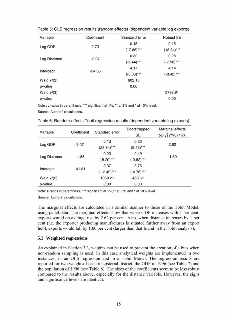
The GLS regression, similar to the OLS, gives an overall indication of the effect on exports of the explanatory variables when using panel data. Table 5 reports the results. The Wald test’s p-values (with varying degrees of freedom) indicate that the model is overall statistically significant at the 1 per cent level. GDP and distance are significant at the 1 per cent level and both have the expected signs. The intercept here is slightly smaller than that of the OLS regression. When considering the results in Table 5, it can be seen that the coefficients on GDP are somewhat smaller, and those of distance quite large. The regression results of the Random-Effects Tobit Model are reported in Table 6. The χ²’s of the Wald test are 1069.21 and 463.67 for the model with standard errors and bootstrapped standard errors respectively. The p-values of the Wald tests are statistically significant at the 1 per cent level, thus the model has a large degree of explanatory power. The sizes of the coefficients, compared to the Tobit Model, are smaller. Again, the coefficients have the expected sign and are statistically significant. The coefficients are smaller in size than that of the OLS and Tobit results in Tables 3 and 4.

2 The Wald test has a χ² distribution under the null hypothesis that all explanatory variables equal zero

(Hou et al. 2005).

15

Table 5: GLS regression results (random effects) (dependent variable log exports)

Variable Coefficient Standard Error Robust SE

Log GDP 2.73 0.15

(17.88)***

0.15

(18.34)***


(-6.44)***

0.28

(-7.50)***


(-8.36)***

4.14

(-8.42)***

Wald χ²(2)

p-value

602.15

0.00

Wald χ²(3)

p-value

3792.91

0.00

Note : z-ratios in parenthesis; *** significant at 1%, ** at 5% and * at 10% level.


Table 6: Random-effects Tobit regression results (dependent variable log exports)

Variable Coefficient Standard error Bootstrapped

SE

Marginal effects


Log GDP 3.07 0.13

(23.84)***

0.33

(9.43)*** 2.62


(-8.20)***

0.49

(-3.82)*** -1.60


(-12.40)***

8.75

(-4.78)***

Wald χ²(2)

p-value

1069.21

0.00

463.67

0.00

Note: z-ratios in parenthesis; *** significant at 1%,** at 5% and * at 10% level.


The marginal effects are calculated in a similar manner to those of the Tobit Model, using panel data. The marginal effects show that when GDP increases with 1 per cent, exports would on average rise by 2.62 per cent. Also, when distance increases by 1 per cent (i.e. the exporter producing manufactures is situated further away from an export hub), exports would fall by 1.60 per cent (larger than that found in the Tobit analysis).

5.3 Weighted regressions

As explained in Section 3.3, weights can be used to prevent the creation of a bias when non-random sampling is used. In this case analytical weights are implemented in two instances: in an OLS regression and in a Tobit Model. The regression results are reported for two weightsof each magisterial district, the GDP of 1996 (see Table 7) and the population of 1996 (see Table 8). The sizes of the coefficients seem to be less robust compared to the results above, especially for the distance variable. However, the signs and significance levels are identical.

16

The marginal effect of distance on exports in the weighted Tobit estimator (using GDP as analytical weight) is considerably smaller than that of the previous results. Here, a 1 per cent increase in distance from an export hub is associated with a decrease in exports of only 0.18 per cent. The marginal effect of GDP on exports is similar (1 per cent increase in GDP creates an increase of 3.27 per cent in exports). Marginal effects are calculated using population as analytical weight with the effect of distance slightly more severe on exports and the contribution of GDP larger.

Table 7: Weighted OLS and Tobit regression results (dependent variable log exports; analytical weight = GDP of 1996)

Regression Weighted OLS Weighted Tobit

Variable Coefficient Standard error Coefficient Standard error Marginal effects


Log GDP 2.50 0.06

(43.61)*** 3.27

0.09

(37.04)*** 3.27


(-6.67)*** -0.18

0.08

(-2.26)** -0.18


(-25.42)*** -56.37

2.26

(-24.95)***

Adjusted R²

Root MSE

0.59

3.73

LR χ²(2)

p-value

Pseudo R²

2089.62

0.0000

0.119

Note: t-ratios in parenthesis; *** significant at 1%, ** at 5% and * at 10% level.


Table 8: Weighted OLS and Tobit regression results (dependent variable log exports; analytical weight = population of 1996)

Regression Weighted OLS Weighted Tobit

Variable Coefficient Standard error Coefficient Standard error Marginal effects


Log GDP 3.08 0.08

(38.24)*** 4.43

0.13

(34.83)*** 4.03


(-38.84)*** -1.08

0.14

(-7.62)*** -0.98


(-22.75)*** -78.79

3.24

(-24.34)***

Adjusted R²

Root MSE

0.59

5.4888

LR χ²(2)

p-value

Pseudo R²

2302.88

0.0000

0.1270

Note : t-ratios in parenthesis; *** significant at 1%, ** at 5% and * at 10% level.


17

It should be noted that although most of the results using surface area as a proxy for domestic transport costs are statistically insignificant, the results from the weighted regressions are not. The results are not reported here, however the sign of surface area is negative and that of GDP is positive. In conclusion, the various estimators used in this article gave results on the signs for the coefficients, positive for GDP and negative for distance. Therefore, the sign and coefficients can be considered as robust (although the size of the coefficient cannot be deemed robust). The effect of GDP (the home-market effect) was also found to be much stronger in all cases than that of distance. The effect of distance, in particular, was found to be sensitive towards the size of the district. When the latter was controlled using analytical weights, the effect of an increase of 1 per cent in distance from an export hub would result in a fall in manufactured exports of approximately 0.18 per cent.

6 Conclusions and recommendations

Nicolini (2003: 447) recently stated that ‘one of the principal unsolved dilemmas of trade theory’ is ‘why and where people decide to locate their production’. In this paper, the question where exporters of manufactured goods would be located within a country was investigated. Based on insights from new trade theory, the new economic geography and gravity-equation modelling, an empirical model was specified wherein agglomeration and increasing returns (the home-market effect) and transport costs (proxied by distance) were identified as major determinants of choice of location for exporters. The main result of this paper is that internal distance and thus domestic transport costs, influences the extent to which different regions in a developing country can be expected to be successful in exporting manufactures. Data from 354 magisterial districts in South Africa were used with a variety of estimators (OLS, Tobit, RE-Tobit) and allowances for data shortcomings (bootstrapped standard errors and analytical weights) to determine that the home-market effect (measured by the size of local GDP) and distance (measured as the distance in km to the nearest port) are significant determinants of regional manufactured exports. The contribution of this paper was to test for these determinants using developing country data, and to generally contribute to the small literature on this topic. In this regard this paper complements the paper of Nicolini (2003) on the determinants of exports from European regions. In particular, it was found here that home-market effect has a much larger or stronger effect on exports (the marginal effect was calculated as between 3.2 and 4) than distance (the marginal effect, when weighted, was between 0.18 and 0.28) in a developing country setting. In contrast, Nicolini (2003: 459, 460, 461) found the effect of the home-market effect to be significant but smaller in overall size and the effect of transport/distance (which she proxied using surface area and transport infrastructure) to be slightly higher, with sizes of coefficients ranging between 0.7 and 1.3 for the home-market effect (GDP) and -0.36 and -0.58 for distance (surface area). Although direct comparisons between the results in this paper and that of Nicolini (2003) for Europe are made difficult due to different estimation methods and different proxies for distance (our measures are more accurate for distance) the overall suggestion is that the home-market effect is relatively more important in the developing country context (South Africa) with more imperfectly competitive firms. This result is

18

consistent with the theoretical model of Puga (1998) wherein developing countries which urbanise later and with ‘better transport technologies’ (such as South Africa) are spatially more concentrated than present developed regions (such as the EU) (Venables 2005: 16). Further research is recommended to investigate the ways in which geography and historical patterns of location may result in regional differences in the relative importance of increasing returns and transport costs.

References

Amemiya, T. (1984). ‘Tobit Models: A Survey’, Journal of Econometrics 24(1-2): 3-61.

Armstrong, H., and J. Taylor (2000). Regional Economics and Policy, third edition, Blackwell Publishers: Malden MA.

Anderson, J.E. (1979). ‘A Theoretical Foundation for the Gravity Equation’, American Economic Review 69: 106-16.

Baltagi, H. (1995). Econometric Analysis of Panel Data, John Wiley and Sons: Chichester.

Bergstrand, J.H. (1985). ‘The Gravity Equation in International Trade: some Microeconomic Foundations and Empirical Evidence’, The Review of Economics and Statistics 67(3): 474-81.

Bergstrand, J.H. (1989). The Generalised Gravity Equation, Monopolistic Competition, and the Factor-Proportions Theory in International Trade, The Review of Economics and Statistics 71: 143-53.

Bergstrand, J.H. (1990). ‘The Heckscher-Ohlin-Samuelson Model, the Linder Hypothesis and the Determinants of Bilateral Intra-Industry Trade’, The Economic Journal 100: 1261-29.

Bosker, M. and W.F. Krugell (2006). ‘Regional Income Evolution in South Africa after Apartheid’, paper presented at the EcoMod Conference, 1-2 June, Brussels.

Bougheas, S., P.O. Demetriades, and E.L.W. Morgenroth (1999). ‘Infrastructure, Transport Costs and Trade’, Journal of International Economics 47: 169-89.

Brakman S., H. Garretsen, and C. van Merrewijk (2001). An Introduction to Geographical Economics, first edition, Cambridge University Press: Cambridge.

Clark, X., D. Dollar, and A. Micco (2004). ‘Port Efficiency, Maritime Transport Costs, and Bilateral Trade’, Journal of Development Economics 75: 417-50.

Coetzee, Z.R., K. Gwarada, W.A. Naudé, and J. Swanepoel (1997). ‘Currency Depreciation, Trade Liberalisation and Economic Development’, The South African Journal of Economics 65(2): 165-90.

Cong, R. (2001). ‘How Do You Compute Marginal Effects After ologit/oprobit/mlogit mfx?’, available from: www.stata.com/support/faqs/stat/mfx_ologit.html, accessed 19 September 2006.

Crafts, N., and A. Mulatu (2005). ‘What Explains The Location Of Industry in Britain, 1871-1931?’, Journal of Economic Geography 5: 499-518.

19

Cribari-neto, F. and S.G. Zarkos (1999). ‘Bootstrap Methods for Heteroskedastic Regression Models: Evidence on Estimation and Testing’, Econometric Reviews 18: 211-28.

Deardorff, A.V. (1995). ‘Determinants of Bilateral Trade: Does Gravity Work in a Neoclassical World?’ NBER Working Paper 5377, National Bureau of Economic Research: Cambridge MA.

DoT (Department of Trade) (2005). National Freight Logistic Survey, available from: www.transport.gov.za/library/docs/policy/freightlogistics/index.html, accessed 12 July 2006.

Evenett, S.J., and W. Keller (1998). ‘On Theories Explaining the Success of the Gravity Equation’, NBER Working Paper 6253, National Bureau of Economic Research: Cambridge MA.

Feenstra, R.C., J.R. Markusen, and A.K. Rose (2001). ‘Using the Gravity Equation to Differentiate among Alternative Theories of Trade’, The Canadian Journal of Economics 34(2): 430-47.

Fosu, A.K. (1990a). Exports and Economic Growth: The African Case, World Development 18(6): 831-5.

Fosu, A.K. (1990b). ‘Export Composition and the Impact of Exports on Economic Growth of Developing Economies’, Economic Letters 34(1): 67-71.

Fujita, M., and P.R. Krugman (2004). ‘The New Economic Geography: Past, Present and the Future’, Papers in Regional Science 83(1): 139-64.

Fujita, M., P.R Krugman, and A.J. Venables (2001). The Spatial Economy, MIT Press: Cambridge MA.

Global Insight Southern Africa (2006). Regional Economic Explorer, Global Insight: Pretoria.

Greene, W.H. (2003). Econometric Analysis, fifth edition, Prentice Hall: New Jersey.

Gries, T., and W.A. Naudé (2007). ‘Trade and Endogenous Formation of Regions in a Developing Country’, Review of Development Economics (forthcoming).

Gujarati, D.N. (2006). Essentials of Econometrics, third edition, McGraw-Hill: Singapore.

Hausmann, R., and B. Klinger (2006). ‘South Africa’s Export Predicament’, CID Working Paper 129, Centre for International Development at Harvard University: Cambridge MA.

Head, K. (2003). ‘Gravity for Beginners’, available from: http://72.14.221.104/ search?q=cache:Zy8MErHwxzQJstrategy.sauder.ubc.ca/head/gravity.pdf +head+ % 22 gravity + for+beginners %22&hl=en&gl=za&ct=clnk& cd=1, accessed 10 August 2006.

Heintz, J. (2003). ‘Out of GEAR? Economic Policy and Performance in Post-Apartheid South Africa’, Political Economy Research Institute Research Brief 2003-1, University of Massachusetts: Amherst.

Hoffmann, J. (2002). ‘The Cost of International Transport, and Integration and Competitiveness in Latin America and the Caribbean’, FAL Bulletin 191.

20

Hou, Y., W. Wang, and W. Duncombe (2005). ‘Determinants of Pay-As-You-Go Financing of Capital Projects: Evidence from the States’, paper prepared for the Association of Budgeting and Financial Management Annual Conference, 10-12 November, Washington DC.

Hsiao, C. (2003). Analysis of Panel Data, second edition, Cambridge University Press: New York.

Hummels, D. (1999). ‘Have International Transport Costs Declined?’, available from: www.nber.org/ ~confer/99/itisi99 /hummels.pdf; accessed 9 June 2005.

Kanbur, R., and A. Venables (eds) (2005). Spatial Inequality and Development, Oxford University Press for UNU-WIDER: Oxford.

Krugman, P.R. (1979). ‘Increasing Returns, Monopolistic Competition and International Trade’, Journal of International Economics 9(4): 469-79.

Krugman, P.R. (1980). ‘Scale Economics, Product differentiation and the Pattern of Trade’, American Economic Review 70(5): 950-9.

Krugman, P.R. (1991). ‘Increasing Returns and Economic Geography’, Journal of Political Economy 99(3): 483-99.

Leclere, M.J. (1994). ‘The Decomposition of Coefficients in Censored Regression Models: Understanding the Effect of Independent Variables on Taxpayer Behavior’, National Tax Journal 47(4): 839-45.

Limão, N., and A.J. Venables (2001). ‘Infrastructure, Geographical Distance, Transport Costs and Trade’, World Bank Economic Review 15(3): 451-79.

McCann, P. (2005). ‘Transport Costs and New Economic Geography’, Journal of Economic Geography 5: 305-18.

McDonald, J.F., and R.A. Moffitt (1980). ‘The Uses of Tobit Analysis’, The Review of Economics and Statistics 62: 318-21.

McPherson, M.A., M.R. Redfern, and M.A. Tieslau (1998). ‘A Re-examination of the Linder Hypothesis: a Random-Effects Tobit Approach’, mimeo, Department of Economics, University of North Texas: Denton.

Naudé, W.A. (2001). ‘Shipping Costs and South Africa’s Export Potential: An Econometric Analysis’, The South African Journal of Economics 69(1): 123-46.

Naudé, W.A., and W.F. Krugell (2003). ‘An Inquiry into Cities and their Role in Subnational Economic Growth in South Africa’, Journal of African Economies 12(4): 476-99.

Naudé, W.A., and W.F. Krugell (2006). ‘Economic Geography and Growth in Africa: The Case of Sub-National Convergence and Divergence in South-Africa’, Papers in Regional Science 85 (3): 443-57.

Naudé, W.A, and M. Matthee (2007). ‘The Geographical Location of Manufacturing Exporters in South Africa’, WIDER Research Paper 2007/09, UNU-WIDER: Helsinki.

Nicolini, R. (2003). ‘On the Determinants of Regional Trade Flows’, International Regional Science Review 26(4): 447-65.

21

Overman, H.G., S.J. Redding, and A.J. Venables (2001). ‘The Economic Geography of Trade, Production and Income: A Survey of Empirics’, available from: http://econ.lse.ac.uk/staff/ajv/hosrtv.pdf; accessed 9 January 2006.

Puga, D. (1998). Urbanization Patterns: Europe versus Less Developed Countries, Journal of Regional Science 38: 231-2.

Radelet, S., and J. Sachs (1998). ‘Shipping Costs, Manufactured Exports and Economic Growth’, available from www.earthinstitute.columbia.edu/about/director/ pubs/shipcost.pdf; accessed 9 June 2005.

Rankin, N. (2001). ‘The Export Behaviour of South African Manufacturing Firms’, presentation delivered at the Trade and Industrial Policy Strategies Forum 2001 New Directions in the South African Economy, 10-12 September, Johannesburg.

Redding, S. and P.K. Schott (2003). ‘Distance, Skill Deepening and Development: Will Peripheral Countries Ever Get Rich?’, Journal of Development Economics 72: 515-41.

Roneck, D.W. (1992). ‘Learning More from Tobit Coefficients: Extending a Comparative analysis of Political Protests’, American Sociological Review 57(4): 503-7.

Roux, A. (2004). Getting into GEAR’, in R. Parsons (ed.) Manual, Markets and Money Double Story Books: Cape Town.

Salvatore, D. (1998). International Economics, Sixth Edition, Prentice Hall: New Jersey.

Samuelson, P.A. (1952). ‘The Transfer Problem and Transport Costs: the Terms of Trade when Impediments are Absent’, Economic Journal 62: 278-304.

Sigelman, L. and L. ZHENG (1999). ‘Analyzing Censored and Sample-Selected Data with Tobit and Heckit Models’, Political Analysis 8(2): 167-82.

Smith, J. (2006). ‘Censored/Truncated Regression Lectures’, available from: www-personal.umich.edu/~econjeff/Courses/ec675_lectures_censored_regression.pdf; accessed 9 October 2006.

STATA (2006). User’s Guide (Release 9), Stata Press Publication: College Station TX.

Suleman, A. and W.A. Naudé (2003). ’The Competitiveness of South African Manufacturing: A Spatial View’, Journal for Studies in Economics and Econometrics 27(2): 29-52.

The Round Table (2004). ‘Transport and International Trade. European Conference of Ministers of Transport: Conclusions of Round Table 131’, available from: www.cemt.org/online/conclus/rt131e.pdf; accessed 1 December 2005.

Tobin, J. (1958). ‘Estimation of Relationship for Limited Dependent Variables’, Econometrica 26(1): 24-36.

UCLA Academic Technology Services (2006). ‘Stata Data Analysis Examples: Tobit Analysis’, available from: www.ats.ucla.edu/stat/stata/dae/tobit.htm; accessed 11 September 2006.

22

Venables, A.J. (2001). ‘Geography and International Inequalities: the Impact of New Technologies’, available from: http://econ.lse.ac.uk/staff/ajv/abcde3.pdf; accessed 3 January 2006.

Venables A.J. (2005). ‘Spatial Disparities in Developing Countries: Cities, Regions and International Trade’, Journal of Economic Geography 5: 3-21.

Verbeek, M. (2000). A Guide to Modern Econometrics, John Wiley: Chichester.

Vogelvang, B. (2005). Econometrics: Theory and Applications with EViews, Prentice Hall: Harlow.

wider research paper 2007/10 the determinants of … · (ols, tobit, re-tobit) and allowances for...

Documents