Why some are more equal than others?

December 2015

E. Díaz-Bonilla and M. Thomas

Country typologies of food security

The State of AgriculturalCommodity Markets

2015-16

Background paper

Why some are more equal than others Country typologies of food security

Eugenio Díaz-Bonilla, Marcelle Thomas

Background paper prepared for The State of Agricultural Commodity Markets 2015–16.

Food and Agriculture Organization of the United Nations Rome, 2015

ii

The designations employed and the presentation of material in this information product do not imply the expression of any opinion whatsoever on the part of the Food and Agriculture Organization of the United Nations (FAO) concerning the legal or development status of any country, territory, city or area or of its authorities, or concerning the delimitation of its frontiers or boundaries. The mention of specific companies or products of manufacturers, whether or not these have been patented, does not imply that these have been endorsed or recommended by FAO in preference to others of a similar nature that are not mentioned. The views expressed in this information product are those of the authors and do not necessarily reflect the views or policies of FAO. © FAO, 2015 FAO encourages the use, reproduction and dissemination of material in this information product. Except where otherwise indicated, material may be copied, downloaded and printed for private study, research and teaching purposes, or for use in non-commercial products or services, provided that appropriate acknowledgement of FAO as the source and copyright holder is given and that FAO’s endorsement of users’ views, products or services is not implied in any way. All requests for translation and adaptation rights, and for resale and other commercial use rights should be made via www.fao.org/contact-us/licence-request or addressed to copyright@fao.org. FAO information products are available on the FAO website (www.fao.org/publications) and can be purchased through publications-sales@fao.org.

iii

Contents

Acknowledgements........................................................................................................................... iv

Executive summary ............................................................................................................................ v

1. Introduction ..................................................................................................................................1

2. Regional aspects ............................................................................................................................1

3. Country typologies ........................................................................................................................4

3.1. Agriculture.............................................................................................................................4

3.2. Food security .........................................................................................................................5

3.2.1. Purpose ................................................................................................................................. 7

3.2.2. Variables ................................................................................................................................ 7

3.2.3. Methods ................................................................................................................................ 9

3.2.4. Groups identified ................................................................................................................ 10

3.3. Some closing comments for this section ............................................................................... 12

4. A country typology of food security conditions ............................................................................. 13

4.1. Objective ............................................................................................................................. 13

4.2. Variables and country coverage............................................................................................ 13

4.3. Method ............................................................................................................................... 14

4.4. Results ................................................................................................................................ 15

4.5. Policy implications ............................................................................................................... 19

5. Conclusion ................................................................................................................................ 24

References ....................................................................................................................................... 25

iv

Acknowledgements This document was commissioned as a background paper for the preparation of the 2015–16 edition of FAO’s flagship report The State of Agricultural Commodity Markets. It was prepared by Eugenio Díaz-Bonilla, Visiting Senior Research Fellow, and Marcelle Thomas, Research Analyst, both at the International Food Policy Research Institute (IFPRI). Its preparation was guided by a terms of reference prepared by FAO. The paper benefited from comments by participants at a series of meetings held by FAO in the first half of 2015 to provide input into the drafting of the report.

v

Executive summary This paper reviews several approaches to create typologies of food (in)security conditions. There may be different objectives for the typologies, which influence the variables selected, methods and the number of groups formed. The definition of the adequate number of groups depends largely on the purpose of the exercise and should be maintained within a limited range that allows a manageable quantity of differentiated policy packages to be outlined. The paper also makes the point that the groups are formed based on selected variables, addressing the criticism that the typology places different countries in the same category. The paper then addresses a specific exercise to build a food security typology using cluster analysis as the classification methodology. The cluster analysis uses five variables: domestic food production per capita (constant dollars per capita); a combination of calories and proteins per capita; the ratio of total exports to food imports; the ratio of the non-agricultural population to total population; and a variable based on the mortality rate for children under five. The raw values are all transformed into z-scores. The paper explains how the variables relate to the traditional dimensions of availability, access and utilization in the definition of food security. Data for the variables correspond to the period 2009–2011 (or the latest available) and include 155 developed and developing countries. Two clustering methods are applied: hierarchical and k-means. The hierarchical approach is used first, to determine potential outliers and to explore what would be a reasonable number of clusters. This analysis allows elimination of three outliers (New Zealand, Argentina and Iceland) and also shows that above ten clusters the differentiation occurred among those groups with clearly better food security indicators. Therefore, for the analysis of food insecurity, those differentiations did not add relevant information and therefore it was considered that ten clusters should suffice to capture the country variations relevant for differentiated policy approaches. The k-means was applied because the hierarchical method, although very useful to define the number of clusters, does not allow for reallocation of countries when those new groups are formed. The k-means, on the other hand, although requiring that the number of clusters be defined from the outset, has the advantage that it allows reallocation of countries as the classification proceeds and different groups are formed. The paper analyses the groups formed and presents the results for the five groups considered food insecure or what is termed “intermediate” food security. The dichotomies of rural/urban configurations and trade stressed/not trade stressed were highlighted and different policies discussed. Limitations related to land and water availability (measured as arable land, hectares per person and renewable internal freshwater resources in cubic metres per capita), were incorporated into the analysis.

1. Introduction This paper looks into the classification of countries with regard to food and nutrition security conditions and discusses different approaches and methodologies. The objective is to identify a number of country groups that can provide some guidance about potential policies to address food and nutrition insecurity. The definition of the adequate number of groups depends largely on the purpose of the exercise, as discussed later. It should be recognized, though, that every country is unique, and therefore policy makers and analysts, when discussing specific policies, must make an effort to understand the country and its circumstances. This implies considering (1) current economic conditions, (2) the totality of the economic programme where the policy being considered fits, (3) structural aspects of the national economy and society, (4) the heterogeneity of economic agents, and (5) the world economic environment within which the country exists. Many policy and analytical mistakes result from considering policies in isolation, without taking into account the five aspects mentioned here (Díaz-Bonilla, 2015a). This paper is structured as follows. After this introduction, the following section uses a traditional categorization based on geographically defined developing regions. For some exercises, this approach may suffice to distinguish food and nutrition (in)security conditions, looking at a variety of structural and contextual conditions. The third section discusses in greater detail some formal exercises that have been used to classify countries based on agriculture and food security variables. It makes the point that the objective of the classification should guide the exercise and that the classifications depend on the variables elected and the method (or methods) applied. A fourth section presents a specific food security typology using cluster analysis as the classification methodology. The final section presents the conclusions.

2. Regional aspects1 An approach with a long history is to differentiate developing countries according to geographical region. This approach has received some support from econometric regressions that found that dummy variables for regions have statistical significance in relation to growth, for example Sala-i-Martin (1997). As a first approach different developing regions are included using the World Bank’s classification (Table 1), highlighting the great variety in structural characteristics of their agricultural sectors. Agriculture in LAC is less important as a percentage of GDP, and the rural population in this region is smaller compared with total population than in other regions. SSA and SA (followed closely by EAP) represent the other extreme, with agricultural production and rural population having larger incidence. Although agriculture is relatively smaller in terms of GDP in LAC, this region, followed by SSA, depends more on agricultural exports. Agriculture appears to be more productive (per unit of labour) and uses more capital (using tractors as a proxy) in ECA, LAC and MENA.

1 This section is based in part on Chapter 3 of Díaz-Bonilla (2015) forthcoming.

2

Table 1: Regional agricultural indicators

Source: Díaz-Bonilla (2015a) using the WDI database, World Bank (2014). Note: Indicators are average 2005–2011, except tractors, which are calculated for 1995–2000.

Roads represent an important indicator of infrastructure, and SA and then EAP show the higher densities of coverage. LAC and ECA have more available arable land per capita (counting rural population) than Asian countries, with MENA and SSA in between. Average holdings are far larger in LAC, and land appears to be distributed more unequally there than in Asia and Africa (Table 2). Although SSA has about double the land availability per capita than Asia, the region also shows the lowest values for the capital/technology and roads indicators, and the average size of the plots farmed is similar to that in Asia. This highlights some of the opportunities in SSA for agricultural production, such as potentially more land to be incorporated into production, but also the constraints the region faces, such as lack of infrastructure and low productive capital.

Category Europe & Central Asia

Latin America & Caribbean

Middle East & North Africa

Africa south of the Sahara

East Asia & Pacific

South Asia

All developing countries

Rural population (% total population)

41.0 22.2 41.6 64.9 54.6 70.1 55.9

Agriculture, value added (% GDP)

8.9 5.6 10.6 16.8 11.4 18.8 10.8

Agriculture value added per worker (constant US$2005)

4 270.2 3 728.3 2 653.8 655.5 673.2 608.8 843.9

Arable land (hectares per rural population)

1.1 1.3 0.4 0.4 0.2 0.2 0.3

Agricultural machinery, tractors per 100 sq. km of arable land

171.1 116.0 137.1 12.8 59.1 103.0 92.9

Fertilizer consumption (kilograms per hectare of arable land)

57.9 101.4 87.6 12.4 371.3 153.5 142.1

Agricultural exports (percent merchandise trade)

10.2 19.9 5.9 16.2 7.9 12.4 11.4

Road density (km of road per 100 sq. km of land area)

22.5 16.1 10.6 6.7 34.4 103.7 26.6

3

Table 2: Land structure: average size of holdings and concentration

Region/country

Average size

(ha)

Gini index

Africaa 2.92 0.53

Asia, Developingb 2.20 0.57

LAC w/Argentinac 87.09 0.82

LAC w/o Argentina 32.53 0.82

USA 186.95 0.64

EUd 27.27 0.59

Japan/Korea 1.12 0.47

Canada 349.07 0.74

Source: Díaz-Bonilla and Robinson (2010), based on calculations using data from the 2000 World Census of Agriculture; FAO (2010). Notes: a. Burkina Faso, Congo (Dem. Rep.), Djibouti, Egypt, Ethiopia, Guinea, Guinea-Bissau, Lesotho, Libya, Malawi, Namibia, Reunion, Uganda; b. India, Indonesia, Iran, Myanmar, Nepal, Pakistan, Philippines, Thailand, Viet Nam; c. Honduras, Panama, Puerto Rico, Argentina, Brazil, Colombia, Paraguay, Peru; d. Austria, Belgium, Denmark, Finland, France, Germany, Greece, Ireland, Italy, Luxembourg, Netherlands, Portugal, Spain and United Kingdom.

More generally, those structural factors will influence the impact of different policies. For instance, trying to improve internal terms of trade for agricultural products (e.g. by a devaluation of the local currency) will have a different production response in SSA, where producers face relatively more constraints in infrastructure, capital and technology, than in Asia or LAC. As a result of the lack of internal infrastructure in SSA countries, the growing urban markets may be in several cases better linked to international food aid and imports than to the producers in the domestic economy. In turn, the distributive effect (and therefore the political economy implications for policies benefiting the agricultural sector) will be different in the small-farmer agricultural economies of Asia than in many LAC countries with dualistic agrarian structures and large populations of urban poor. In the latter countries, trade and macroeconomic policies improving relative prices for agriculture, at least on impact, may benefit large farmers relatively more than smaller ones, and may have potentially negative impacts on poor urban consumers. Therefore, the political economy of different policies will differ across those regions. The Global Hunger Index (GHI)2 (IFPRI, Concern Worldwide, and Welthungerhilfe, 2014) gives another view of the heterogeneity across developing regions, now based on indicators of food security. For instance, South Asia and SSA show values above 18, when the average value for the developing world is 12.5 (as mentioned in the footnote, a higher number reflects worse hunger conditions), while LAC, and Eastern Europe and Central Asia, present the more favourable conditions (values about or below four), with the other regions in between.

2 The International Food Policy Research Institute (IFPRI), Concern Worldwide, and Welthungerhilfewith developed a Global Hunger Index that attempts to reflect the multidimensional nature of hunger, combining three equally weighted indicators into one index: (1) the proportion of undernourished people as a percentage of the population (calculated by FAO); (2) the proportion of children younger than five years of who have low weight for their age; and (3) the mortality rate of children younger than five (see IFPRI, Concern Worldwide, and Welthungerhilfe 2014). The GHI is calculated as the simple average of those three indicators. The largest (and worst) theoretical value is 100, which would represent the (largely impossible) situation in which the whole population was undernourished, all children under five were underweight, and all children died before reaching five years of age. The best value would be zero, in the (also unlikely) situation in which there are no persons in any of the three categories described.

4

In summary, using Tables 1 and 2, and the GHI index, it seems possible to characterize the main regions with data as in the next Table 3. Table 3: A Summary of regional characteristics

GHI Agriculture Agrarian structure

Infrastructure Urbanization

LAC Better Less incidence in GDP but more on exports

Larger farms, highly unequal

Better Urban

SSA Worse More incidence in GDP but less on exports

Smaller farms; more equal agrarian structure

Worse Rural

Asia Worse SA, intermediate ESEA

More incidence in GDP, intermediate on exports

Smaller farms; more equal agrarian structure

Better Rural

Source: authors A geographical classification can provide a guide to the discussion of differentiated policy approaches for some aggregate analyses of food and nutrition security. However, for more specific policy discussions a finer disaggregation may be needed that considers individual countries. This is discussed.

3. Country typologies

3.1. Agriculture The 2008 World Development Report from the World Bank (2007), which focused on agricultural development issues, divided developing countries into three groups depending on two variables: the contribution of agriculture to growth and the importance of rural poverty. It used a clustering method based on the two variables considered. This approach allowed the definition of relevant groupings of countries, but at the same time the number of groups was kept at a manageable level for the type of policy analysis that was intended: just three categories were identified. They were called 1) agriculture-based countries, where agriculture contributes significantly to growth and where the poor are concentrated in rural areas; 2) transforming countries, where agriculture contributes less to growth but where poverty is still predominantly rural; and 3) urbanized countries, where agriculture is not the main contributor to growth and where poverty is mostly urban. Based on these characteristics, the analysis suggested differentiated sets of agricultural policies for the three groups of countries (World Bank, 2007). This is an example of a classification exercise that, based on a small set of relevant variables, comes up with a limited number of groups that are relevant for the policy issues addressed. Although the classification is done at the level of countries, the three categories can be approximately mapped into general income and geographical groupings, as in the previous section. For instance, in general, low- and lower-middle-income countries, many from Africa south of the Sahara (SSA), represent the largest percentage in the first group. Lower-middle- and middle-income countries from South Asia

5

(SA), East Asia and the Pacific (EAP), and to a lesser extent the Middle East and North Africa (MENA), belong in the second category. Finally, middle- and upper-middle-income countries, mostly from Latin America and the Caribbean, as well as from Eastern Europe and Central Asia (ECA), are the main income groups and geographical regions in the third category. Therefore, although general geographical classifications provide some differentiation regarding agricultural conditions (in this case) and potential policies, country classifications add further details to the understanding of different conditions and policies.

3.2. Food security There are several approaches used to categorize food and nutrition (in)security conditions. One approach is based on single-value indicators, such as the Global Food Security Index, designed and constructed by the Economist Intelligence Unit and sponsored by DuPont.3 They are useful to gather quantitative information from different sources, to summarize the situation within a single country, to allow some types of comparison across countries, to increase public awareness about the current situation regarding a specific topic, to look at their evolution over time, and to help policy makers focus on some issues that may require specific attention. However, because they aggregate a series of variables in a single number, they do not capture the differing underlying “geometries” of the indicators: countries may have the same overall number due to a completely different combination of the different variables that have been averaged or aggregated (Díaz-Bonilla, Orden and Kwieciński, 2014). Other approaches are based on classificatory techniques that try to capture the multidimensional geometry of food and nutrition security and allow for the differentiation of profiles. The focus of this section is on those multidimensional classifications. There have been several attempts to produce typologies of food and nutrition security. Those exercises differ in terms of the purposes of the typology, the number of variables considered, the methodology used, and the number of groups or types identified. Here the focus is on four exercises (1) Pieters, H., Gerber, N., and Mekonnen, D., (2014); 2) Yu, B., You, L., and Fan, S., (2010); 3) Matthews, A., (2013); and 4) Díaz-Bonilla, E., Thomas, M., Robinson, S., and Cattaneo, A.. 2000. Table 4 explains some of the main characteristics of the four approaches.

3The GFSI aggregates 28 variables into a single indicator. It also reports 7 “background variables.”

6

Table 4: A summary of different typologies Different Typologies

Purpose Number of variables considered

Methodology Types identified

Matthews Identify categories of countries for case studies for the OECD on trade and food security

35 variables, plus 7 variables termed "helper indicators"

Countries are classified based on thresholds defined by the author and then they are placed in nested tables in a sequential approach. Classifications in tables vary depending on which is the first (or root) criteria used in rows and columns

240 cells or groups, of which 78 have countries in them

Yu, You and Fan

The typology tries to identify "which countries face similar food security situations and therefore might be able to learn from each other’s successes and failures," emphasizing the medium and long term aspects related to production

9 variables, of which 3 (calories, proteins, and fat) are aggregated by principal component analysis; two of the variables related to climate appear to also be aggregated, but it is not clear. In that case, there will be 6 operational variables

Uses principal component analysis to aggregate 3 indicators of availability. The other variables are utilized directly to classify countries based on thresholds defined by the authors and then placed in nested tables in a sequential approach

64 cells or groups in table, and 53 have countries in them

Pieters, Gerber and Mekonnen

The typology will "help policy makers in developing the right strategy as it facilitates the interpretation and drawing of suitable conclusions from case studies and successful policies in other countries ..." and "will help calibrating models and interpreting results at national levels, as well as guide the selection of case studies by project partners."

27 variables, but they are aggregated by principal component analysis into 9 dimensions (see Methodology)

Uses principal component analysis to aggregate a variety of indicators for the following dimensions: food security, nutrition security, obesity, agricultural potential, agricultural performance, economic performance, health infrastructure, political conditions, and innovation conditions. Then the values of the countries for each dimensions are utilized to classify countries based on thresholds defined by the authors constructing nested tables in a sequential approach

The Table for food security (Table 3) defines 128 different cells or groups, of which 40 have countries in them. There are other classification tables using nutrition security, or obesity as the root criterion.

Díaz-Bonilla, Thomas, Robinson and Cattaneo

Determine whether WTO categories for different types of treatment under WTO legal texts (including the SDT for developing countries) reflected underlying food (in)security characteristics

5 variables Cluster analysis 4 basic and 12 disaggregated groups

Source: authors

7

3.2.1. Purpose A first point to be noted is that the exercises differ in their purposes: there may be different ways of classifying countries depending on the reasons for the typology. Matthews (2013) classifies countries in order to define representative case studies for a larger OECD exercise on adequate trade policies for food security. Yu, You and Fan (2010) and Pieters, Gerber and Mekonnen (2014) suggest that their groupings may be used for the consideration of general policies for food and nutrition security and for comparisons across countries. On the other hand, Díaz-Bonilla et al., 2000 have more limited objectives: given that many types of countries, both developed and developing, claimed food security reasons for some type of special consideration under WTO trade agreements, this exercise focused on whether the WTO country categories used to define differentiated commitments in trade negotiations correlated with groups of countries classified on the basis of some general characteristics of food (in)security.4

3.2.2. Variables The second issue, in part related to the objectives, is the selection and measurement of variables. Matthews (2013) and Pieters, Gerber and Mekonnen (2014) use the largest number of variables. Matthews (2013) includes a very helpful database with all the variables, and an Excel file that allows the user to generate different types of classification. Pieters, Gerber and Mekonnen (2014) reduce the dimensionality by aggregating them into nine dimensions: food security, nutrition security, obesity, agricultural potential, agricultural performance, economic performance, health infrastructure, political conditions and innovation conditions. It should be noted that this classification includes obesity indicators, which none of the other exercises do (see Table 5).

4 Other exercises focused on WTO categories include Kasteng, J., Karlsson, A. and Lindberg, C., (2004) (which is

based on Díaz-Bonilla et al., 2000, but adds some further subdivisions of countries) and Ruffer, T., Jones, S. and Akroyd, S., (2002).

8

Table 5. Example 1 – Possible variables to generate country classifications

Food security profile Economic performance profile Share of animal protein in diet Gini Average daily calorie intake GDP per capita Food deficit Women economic opportunity index

Nutrition security profile Political profile Undernourishment Political stability and violence Anaemia women Control of corruption Child mortality Democracy index

Obesity Innovation profile Female obesity Innovation system

Agricultural potential profile Economic incentive regime Length of growing period Education and skills Percentage without major soil constraints Information infrastructure

Precipitation Health infrastructure profile

Agricultural performance profile Health expenditures per capita Value added per worker in agriculture Sanitation Import share of agriculture Water supply Food production per capita Hospital beds

Source: authors, based on variables explained in Pieters, Gerber and Mekonnen (2014).

Yu, You and Fan (2010) mention nine basic variables, but then the three measures of average availability (for calories, proteins and fat) are aggregated by principal component analysis into a single variable and two of the variables related to climate appear also to be aggregated in the analysis (see Table 6).

Table 6: Example 2 – Possible variables to generate country classifications

Food consumption Daily calorie intake per capita (Energy intake per capita per day measured in calories) Daily protein intake per capita (Protein intake per capita per day measured in grams) Daily fat intake per capita (Fat intake per capita per day measured in grams)

Food production Annual food production per capita (Gross sum of all commodities weighted by 1999–2001 average international commodity prices, then divided by total population)

Food imports Ratio of total exports to food imports (Value of all exported goods and market services divided by food imports)

Food distribution Share of urban population (Percentage of midyear population of areas defined as urban in total population)

Agricultural potential Soil without major constraints (Percentage of soil not affected by eight major fertility constraints) Length of growing period (Number of days of the year when both natural moisture and temperature conditions are suitable for crop production) Coefficient of variation of length of growing period Coefficient of variations of length of growing period

Source: authors, based on variables defined in Yu, You and Fan (2010). The point that the objectives of the typology drive the indicators is exemplified by Díaz-Bonilla et al., 2000: they acknowledge “that the deeper issue of nutrition insecurity requires analyses at the

9

household and individual levels,” but the study “takes nonetheless a national perspective (the level at which the negotiating categories are defined) and focuses mainly on food availability issues, using consumption, production, and trade measures.” The five indicators of food security are: calories per day per capita; proteins per day per capita (grams), food production per capita (measured in constant US$ 1989–1991); the ratio of total exports (merchandise and services) to food imports; and the share of non-agricultural population over total population.5 Other indicators, potentially very important for a different type of exercise (such as those used in the papers previously mentioned), were consciously excluded: this is the case for the FAO measure of undernourishment (which is a measure of calorie availability doubly corrected by age/gender and by income distribution), of measures related to health infrastructure, women’s education, and/or indicators of anthropometric outcomes at the individual level (such as wasting or stunting in children). The reasons for the exclusions were that these indicators reflect issues that are related to policies other than trade measures (such as public investments in health or in women’s education) and/or that it would be inadequate that those indicators be used to claim special trade treatment (for instance, no country would attempt to request special trade considerations because it has a very unjust income distribution that worsens FAO’s undernourishment measure, or because women are discriminated against). However, many of the variables not included in Díaz-Bonilla et al.,2000 must be considered if the issue is to identify general policies to address food and nutrition security problems, as in Yu, You and Fan (2010) and Pieters, Gerber and Mekonnen (2014).

3.2.3. Methods The four analyses differ also in the way the groups or types are constructed. While Díaz-Bonilla et al., 2000 use cluster analysis, the other three exercises (Matthew, 2013; Yu, You and Fan, 2010; and Pieters, Gerber and Mekonnen, 2014) use some form of hierarchical and sequential construction of tables with different cells that represent the country groups of food and nutrition security. To construct those groups, the exercises define, in different ways, the cutoff values used to separate groups by each variable or groups of variables. The thresholds between categories may be defined in the original units of the variables, or by converting the original variables into z-scores.6 Except for Matthews (2013) the other three exercises use z-scores at some points to define thresholds and/or to perform calculations. For the cluster analysis in Díaz-Bonilla et al., 2000 this conversion is necessary to avoid giving more weight to any one variable because of its unit of measure. In the three cases that use a hierarchical and sequential construction of tables, key issues to consider

(as noted by Matthews 2013) are a) how many levels/dimensions will be used to generate the classification (too many levels/dimensions would create a large number of types or categories; he suggests that not more than four or five levels would be reasonable); and b) which dimension/variable to choose as the “root” to start the classification. Both Matthews (2013) and Pieters, Gerber and Mekonnen (2014) present different tables depending on which dimension/variable acts as the root of the classification (for instance, Pieters, Gerber and Mekonnen

2014 present three different tables, using food security, nutrition security and obesity indicators as the initial classificatory dimension). While groups would differ depending on the root dimension used, once the mutually exclusive roots or starting points have been selected, then the sequence in which the additional levels/dimensions are added should not matter for the definition of the final groups, provided that those levels/dimensions are the same (in other words, for a given root

5 The last two variables have been inverted from the more common representations (i.e. food imports over

total exports and percentage of rural population) so in all the variables a larger number is considered to be associated with better food security (this also helps to visualize better the charts and tables). 6 The latter is calculated by subtracting the mean and dividing by the standard deviation of a specific variable,

which transforms the original data into a new variable with a zero mean and one (1) standard deviation.

10

dimension and the same additional levels of classifying levels, the final groups would be the same, even though the tables would be visually different with each sequence). The three exercises that use tables built in a hierarchical and sequential fashion differ in the way the individual variables are aggregated or used. Matthews (2013) uses the raw data for the individual variables; Yu, You and Fan (2010), use principal component analysis to aggregate the average level of daily availability of calories, proteins, and fat per capita, but then the other variables are used individually (i.e. they are not aggregated, except perhaps for some of the variables related to climate) and the thresholds are defined using z-scores. Pieters, Gerber and Mekonnen (2014), in turn, use principal component analysis to aggregate a larger number of variables in each of the nine dimensions mentioned before (except obesity, which has only one variable, the other dimensions have three or four variables for each one, and therefore principal component analysis helps to reduce the dimensionality). As noted, Díaz-Bonilla et al., 2000 use cluster analysis, which places all the dimensions/levels on the same footing. As in the other approaches, which variables are considered still matters for the typology.7

3.2.4. Groups identified The types, classes, or groups identified differ significantly in number. Matthews (2013) shows 240 cells (or groups) in the classifying table, with a total of 78 types/groups with countries in them while the rest of the cells are empty (i.e. no country appears in them); Yu, You and Fan (2010) have 64 cells/groups in the table, and 53 types have countries in them; and Pieters, Gerber and Mekonnen (2014) present a table with 128 different cells/groups, and there are 40 mutually exclusive types with countries in them. On the other hand Díaz-Bonilla et al., 2000 used three methods of cluster analysis (hierarchical, k-means, and fuzzy) to classify 167 countries, both developed and developing, encompassing all income levels, into clusters. Then, using the z-scores for variables considered, those clusters were labelled as food insecure ones (those clusters for which the average value of the variables considered fell below -0.58), food neutral (approximately between -0.5 and +0.5), and food secure (approximately above +0.5). Díaz-Bonilla et al., 2000 first identified four clusters (whose profiles for each variable are shown in Figure 1), which they labelled food insecure (cluster 4-1), food neutral (4-2), food secure (4-3) and very food secure (4-4).9

7 A common and mistaken criticism of typologies of any type of entity (countries in this case) is that the groups

formed classify together entities that are very “different.” This issue emerges because usually the critic has in mind some other variable, not used in the classification, to define why countries are “similar” or “different.” The types, groups, or classes defined are comparable, or not, only with regard to the variables considered. Including other variables will produce other typologies. 8 Remember that all the variables have been normalized to z-scores with a mean of zero and a standard

deviation of one. A negative (positive) value means that the cluster is below (above) the mean. Considering that the standard deviation is unity, the classification could have been based on plus or minus one. Alternatively, any value below the mean could have reflected food insecurity. The first would have led to a more restrictive definition of food insecurity and the latter a broader definition. In the end, it was considered better to use -0.5 as an intermediate cutoff value between both options to label groups. 9 Cluster 4-4 was termed very food secure because the average values for the variables were above the

standard deviation of one.

11

Figure 1: Profile of four clusters

Source: Figure 5 page 37 in Díaz-Bonilla et al., 2000. Those four groups were further subdivided into 12 groups, which were classified again depending on whether the average value for the variables in the groups fell below -0.5, between -0.5 and +0.5, and above +0.5. Figure 2 shows the categorization of the 12 clusters using the combined value of average availability of calories and proteins per capita (avcalpro) on one axis, and the ratio of total exports over food imports (exptoimp) on the other.10 The -0.5 line is emphasized in darker tones, and then the +0.5 is shown in lighter tones. Figure 2: Classification with 12 clusters

Source: Figure 10 page 43 in Díaz-Bonilla et al., 2000. Note: “avcalpro” is the normalized value (z-value) of the average availability of calories and proteins per capita and “exptoimp” is the normalized value (z-value) of the ratio of total exports over food imports.

10

The other two variables used in the clustering cannot be shown in a two-dimensional figure.

12

In Figure 2 the food insecure clusters are 1 to 4, the food neutral 5 to 8, and the food secure 9 to 12. As mentioned, the use of classification methods such as cluster analysis allows differentiation of the shape or geometry of the components of food (in)security when compared with single indicators. If all variables have been combined in a single number, different values in the five dimensions may have resulted in the same overall single index, but this would have obscured the existing differences. For instance, cluster 4 has average availability of calories and proteins (it is placed at the zero value for the z-score of the 167 countries), but it is below the -0.5 standard deviation for the trade variable, while cluster 3 is clearly below the average for availability of calories and proteins, but it is a the average of the trade variable (the zero value on the horizontal axis, meaning that these countries are at the world average when considering the percentage of their exports needed to buy food). Therefore, in the terminology of Díaz-Bonilla et al., 2000, the latter group appears “consumption vulnerable”, but not “trade stressed,” while, considering those dimensions, cluster 4 appears to be a mirror image: they are trade stressed (that is, they use a large percentage of their exports to buy food) but they are less consumption vulnerable (their current levels of calories and proteins per capita are close to the average for all countries considered). The policy options for these two types of country may be different: for instance, although both would be helped by producing more, the first group may also increase imports to improve availability of calories and proteins, whereas the second group may be more constrained in that regard. Díaz-Bonilla et al., 2000 used the cluster analysis to draw some general implications for WTO categories. They argued that a) the category of LDCs did a better job at identifying the food insecure; b) the category of NFIDCs did not seem to be as good an indicator of food insecurity because one third of the countries covered in the analysis fell within the food neutral band; c) there were several countries in the food insecure groups that were not included in either of the two previous categories; d) the countries in the WTO category of developing countries appeared spread over all clusters, except the most food secure, so it seemed an inadequate guidance to define special and differential treatment in the negotiations; and e) developed countries were in the food secure category (with some minor exceptions that appeared in the food neutral category). Therefore, claims of food security as a trade concern in developed countries seemed to refer to something very different from what was happening in extremely food insecure countries and that mixing completely different perceptions did not help poor countries.

3.3. Some closing comments for this section The revision of the different typologies suggests several additional comments. First, there are no “general” typologies, rather they are specific to the objectives of the exercise, which must be clear from the start. Second, the objectives drive the variables considered. For instance, if the objective is to analyse trade policies and food and nutrition security, the variables considered may be different than for other exercises focused on more general policy issues. Third, to be useful in policy terms the typology cannot exceed some reasonable low number of types and categories, and the distinctions should help to clarify differential policy and structural issues. The next section presents an exercise to establish a country typology that extends and updates Díaz-Bonilla et al., 2000.

13

4. A country typology of food security conditions

4.1. Objective The objective of this exercise is to support general policy analysis, with an emphasis on trade issues, but trying to maintain the number of groups within a limited range that allows the outlining of a manageable quantity of differentiated policy packages. However, it must be remembered, as noted earlier, that for specific policy advice, every country is unique and must be analysed considering its specificity.

4.2. Variables and country coverage Five variables are used, three of which are similar those used by Díaz-Bonilla et al., 2000: food production per capita (constant dollars per capita), the ratio of total exports to food imports, and the ratio of the non-agricultural population to total population. As before, the raw values are all transformed into z-scores. The first variable (food production per capita) reflects the domestically produced part of food availability, the first component of food security. The second (the ratio of total exports to food imports) reflects access, the second component of food security, but at the country level. The ratio of non-rural population was maintained because, as argued in Díaz-Bonilla et al., 2000 food security challenges and related policies differ in mostly urban or mostly rural countries, reflecting the old policy dilemma of sustaining high food prices to help availability (considering the situation of the producers) or maintaining affordable prices to facilitate access (considering the situation of the

consumers) (see Timmer, Pearson and Falcon 1982 and Díaz-Bonilla 2015a). Then the variables related to calories per capita (kcal/caput/day) and protein per capita (g/caput/day), which were separated in Díaz-Bonilla et al., 2000, are here combined in a single term, Calories and Proteins per capita: the raw values are transformed into z-scores and then averaged for the composite variable. They reflect overall availability, coming from both domestic production and trade. The fifth variable is based on the mortality rate for children under five, which is used to construct what can be termed the “non-mortality” rate: for instance if the under-5 mortality rate in a country is three percent, the variable used is 97 percent11 (i.e. the complement to 100 percent showing the percentage of under-5 children that survived). In this way the convention that larger numbers indicate better conditions is maintained. It is also transformed into a z-variable with zero mean and one standard deviation. Given the more general policy nature of this exercise (which includes trade, but it is not exclusively a WTO-focused analysis), it was considered important to include a variable with anthropometric measures. The latter reflects (albeit along with other factors) the impact of food insecurity at the individual level, particularly regarding aspects related to food access and utilization (the second and third components of food insecurity). There are other potential indicators reflecting poverty and access issues related to food security, such as the rates of children stunting and wasting. However, they were available for a smaller number of countries compared with child mortality, so this last indicator was preferred, having a larger coverage of countries in this exercise.

11

Mortality rates are usually computed in per thousands of born children. The example in percent terms is just to explain the construction of the variable.

14

Data for the variables correspond to the period 2009–2011 (or the latest available) and are from the FAO database (FAOSTAT, 2015) and the World Bank database (World Bank, 2015). Data cover 155 countries, both developed and developing. But as discussed below, Argentina, Iceland and New Zealand were dropped as outliers, and therefore 152 countries are included in the final clusters.

4.3. Method Two clustering methods are applied: hierarchical and k-means.12 The agglomerative hierarchical method starts by assigning a country in its own cluster (i.e. the process starts with as many clusters as countries). Clustering begins by combining the two countries that are the most similar. After the first step, the combination may be a country and a cluster and with further steps clusters may be eventually combined. To measure the changes in similarity within clusters resulting from the agglomeration process, an agglomeration coefficient is computed using the within-cluster minimum variance, or Ward's method. The clusters are joined together so as to minimize the variance at each step (see Appendix I in Díaz-Bonilla et al., 2000 for more details). The hierarchical approach was used first, to get a sense of potential outliers, and to explore what would be a reasonable number of clusters. It must be noted that the number of groups depends on the uses of the typology and requires some decisions by the analyst as to the number of clusters most appropriate in a particular analysis. This decision is helped by some statistical indicators, but requires judgment.13 Here, as in Díaz-Bonilla et al., 2000, the hierarchical method is used to decide about the number of groups, by running a sequential classification starting with two clusters (a bare minimum for policy analysis) and going up to 15 clusters (which was considered beyond what would be a manageable number of groups for differentiated analysis. Also, that level of disaggregation generated further divisions of countries without clear policy implications for food insecurity as discussed below). Then the country composition of each of the two to 15 countries was analyzed looking for 1) stable groupings, 2) at what number of clusters some groups were formed, and 3) the presence of outliers. The existence of outliers may be due to extreme values of some variable or to the particular combination of variables instead of the value of any single one of them. It was clear that New Zealand, Argentina and Iceland were outliers classified consistently in single-country clusters by the hierarchical method once a reasonable number of groups began to form, and were dropped from the final sample. Also, it was found that above ten clusters the differentiation happened among the groups with clearly better food security indicators. Therefore, for the analysis of food insecurity, those differentiations did not add relevant information. Ultimately, it was considered that ten

12

In Díaz-Bonilla et al., 2000 a third method was used, Fuzzy cluster analysis (developed by Sherman Robinson and Andrea Cattaneo). In some regards it is similar to the k-means, but the latter is categorical in its cluster partition (i.e. the objects being classified, countries in this case, are either in a group or they are not), while the Fuzzy algorithm allows degrees of membership in different groups. While the k-means indicates how similar or dissimilar from the centre of a cluster a member in that cluster may be, the Fuzzy cluster analysis incorporates information about what is the dominant degree of membership in a particular cluster, but also the degree of belonging to other clusters. In terms of the final classification (i.e. to what cluster a country belonged), the k-means method and the dominant cluster in the Fuzzy method generated similar allocation of countries to clusters (i.e. there were no divergences in the country composition of the clusters analyzed). Therefore, here only the k-means approach is used. 13

The exercises discussed in the previous sections that did not use cluster analysis also had to generate decisions regarding the number of dimensions needed for their analyses, which defined the final number of country groups.

15

clusters should suffice to capture the variations in food security conditions that suggested differentiated policy approaches.14 Then the k-means was used to refine the process of the country classification, considering that the hierarchical method, although very useful to define the number of clusters, does not allow for reallocation of countries when those new groups are formed. The k-means, on the other hand, although requiring that the number of clusters be defined from the outset, has the advantage that it allows reallocation of countries as the classification proceeds and different groups are being formed. This method allocates objects to clusters so as to minimize an expression that includes the sum of Euclidean distances over all objects and clusters; countries are reclassified as the cluster centres are recalculated with new members. But, as noted above, the k-means approach depends on the hierarchical method to define the number of clusters and to specify the starting average value for the variables in each cluster (also called clusters seeds or centroids). All objects that are closest to a particular profile of centroids are assigned to the corresponding cluster. In a first iteration, all countries are assigned to the number of clusters defined. But given that the countries now in that cluster may be different from the ones used by the hierarchical method to calculate the starting values of the centres, the latter may have changed. Then, the new centres are recomputed, and in subsequent iterations the countries are reassigned, changing again the cluster membership and the cluster centres. The procedure stops when successive iterations do not change the centres more than a very minimum threshold value (such as 0.0001). In this exercise the k-means method converged rapidly (see Appendix I in Díaz-Bonilla et al., 2000 for more details on the methodology).

4.4. Results Tables 7, 9 and 10 show the results of the typology, divided into food insecure, food neutral and food secure groups respectively. The groups are ordered considering the values of the variables. The tables present the average z-scores for the five variables explained before and for each cluster. Values smaller than -0.5 are shown in red; those between -0.5 and 0 are in yellow, between 0 and +0.5 in white, and above +0.5 in green. Each table also shows the simple average of the z-scores for the five variables and the number of countries in the cluster. The list of developing countries in each cluster is included in the footnotes.15 Table 7 shows the clusters of countries considered food insecure in this typology.

14

The number of clusters selected is partly a function of the desired level of similarity among members of the same cluster. A useful device for that analysis is the dendrogram, a chart that provides a graphical view of the agglomeration process and shows the increase of the agglomeration coefficient at each level of agglomeration. Initially, when every country is in its own cluster, the value of the coefficient is zero and it increases as the number of clusters is reduced by joining them together. Díaz-Bonilla et al.. 2000 found that the agglomeration coefficients were small (higher similarity within clusters) up to the ten-cluster level of agglomeration, but that those coefficients started to increase in larger jumps after that level. This suggested that each of the clusters were becoming less similar internally if the number of clusters was reduced to fewer than ten, and particularly when moving to fewer than four clusters. 15

Developed countries, defined as all those with an income per capita according to the World Bank Atlas method that was higher than that for Saudi Arabia, are not shown in the footnotes, even though they were part of the cluster exercise. They include the following 27 countries: Australia, Austria, Belgium, Brunei Darussalam, Canada, Denmark, Finland, France, Germany, Greece, Ireland, Israel, Italy, Japan, Republic of Korea, Kuwait, Luxembourg, Netherlands, Norway, Portugal, Slovenia, Spain, Sweden, Switzerland, United Arab Emirates, United Kingdom and United States of America.

16

Table 7: Food insecure clusters

Variables Food insecure clusters

1 2 3 4

Under-5 mortality -1.45 -2.44 -0.5 -0.03

Food production (%) -0.58 -0.62 -0.14 -0.35

Calories and proteins (%) -0.78 -0.86 -0.16 -0.47

Total exports per food imports -0.76 1.02 4.2 -0.49

Non-agricultural population -1.03 -0.68 -0.78 -1.42

Average value of indicators -0.92 -0.716 0.524 -0.552

Number of countries in cluster 3216 417 218 1319

Source: authors, based on the results of the cluster analysis Cluster 1 has an average for the five variables that is clearly below -0.5. It should be emphasized that the average is for the cluster, not for each of the individual countries. However, the cluster algorithm calculates that the 32 countries included in Cluster 1 are “closer” to the average profile indicated in Table 7 than countries in other clusters. They are rural countries that have worrisome indicators for under-5 mortality, production per capita, availability of calories and proteins per capita and the burden of food imports over total exports. Cluster 2 is similar to Cluster 1 in most regards, but differs in that its members do not suffer a burden of food imports. While Cluster 1, using the terminology in Díaz-Bonilla et al., 2000 indicates severe trade stress, Cluster 2 indicates a large margin to increase food imports if the countries in that group decide to use that approach to improve food availability. Cluster 3 is special because it contains only two countries, India and Turkmenistan. Table 8 allows a better look at the individual profiles. Table 8: Analysis of Cluster 3

India Turkmenistan Cluster 3

Under-5 mortality -0.53 -0.47 -0.5

Food production (%) -0.52 0.24 -0.14

Calories and proteins (%) -0.76 0.44 -0.16

Total exports per food imports 4.15 4.25 4.2

Non-agricultural population -1.18 -0.38 -0.78

Source: authors, based on the results of the cluster analysis India and Turkmenistan appear to have been clustered together because they have very small food import bills, which give a large value to total exports per unit of imported food (a value of more than

16

The countries included in this cluster are Afghanistan, Benin, Burkina Faso, Cameroon, Central African Republic, Côte d'Ivoire, Ethiopia, Gambia, Ghana, Guinea, Guinea-Bissau, Haiti, Kenya, Lao PDR, Lesotho, Liberia, Madagascar, Malawi, Mali, Mauritania, Mozambique, Niger, Pakistan, Rwanda, Senegal, Sierra Leone, Swaziland, Timor-Leste, Togo, Uganda, United Republic of Tanzania and Zimbabwe. 17

The countries included are Angola, Chad, Nigeria and Zambia. 18

The countries included are India and Turkmenistan. 19

The countries included are Bangladesh, Cambodia, Guyana, Kyrgyzstan, Myanmar, Nepal, Solomon Islands, Sri Lanka, Tajikistan, Trinidad and Tobago, Uzbekistan, Viet Nam and Yemen.

17

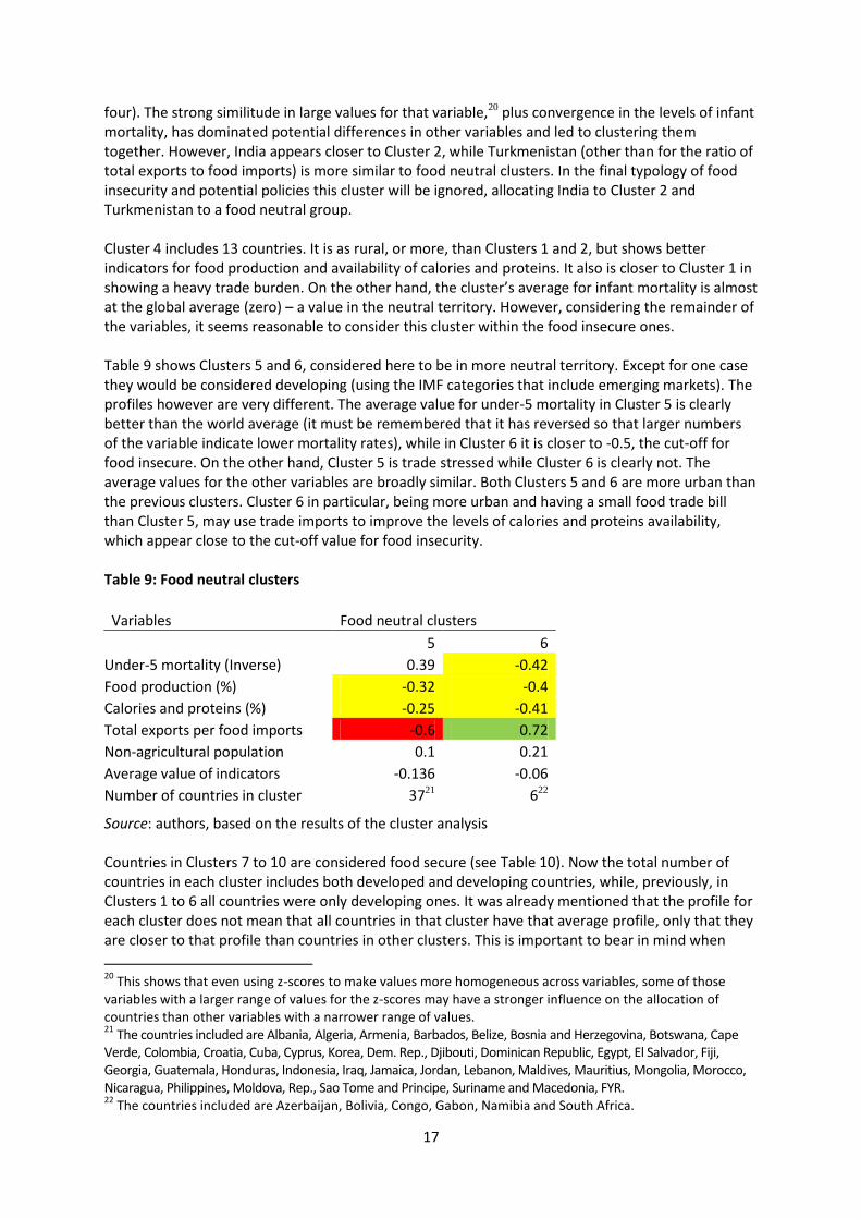
four). The strong similitude in large values for that variable,20 plus convergence in the levels of infant mortality, has dominated potential differences in other variables and led to clustering them together. However, India appears closer to Cluster 2, while Turkmenistan (other than for the ratio of total exports to food imports) is more similar to food neutral clusters. In the final typology of food insecurity and potential policies this cluster will be ignored, allocating India to Cluster 2 and Turkmenistan to a food neutral group. Cluster 4 includes 13 countries. It is as rural, or more, than Clusters 1 and 2, but shows better indicators for food production and availability of calories and proteins. It also is closer to Cluster 1 in showing a heavy trade burden. On the other hand, the cluster’s average for infant mortality is almost at the global average (zero) – a value in the neutral territory. However, considering the remainder of the variables, it seems reasonable to consider this cluster within the food insecure ones. Table 9 shows Clusters 5 and 6, considered here to be in more neutral territory. Except for one case they would be considered developing (using the IMF categories that include emerging markets). The profiles however are very different. The average value for under-5 mortality in Cluster 5 is clearly better than the world average (it must be remembered that it has reversed so that larger numbers of the variable indicate lower mortality rates), while in Cluster 6 it is closer to -0.5, the cut-off for food insecure. On the other hand, Cluster 5 is trade stressed while Cluster 6 is clearly not. The average values for the other variables are broadly similar. Both Clusters 5 and 6 are more urban than the previous clusters. Cluster 6 in particular, being more urban and having a small food trade bill than Cluster 5, may use trade imports to improve the levels of calories and proteins availability, which appear close to the cut-off value for food insecurity. Table 9: Food neutral clusters

Variables Food neutral clusters

5 6

Under-5 mortality (Inverse) 0.39 -0.42

Food production (%) -0.32 -0.4

Calories and proteins (%) -0.25 -0.41

Total exports per food imports -0.6 0.72

Non-agricultural population 0.1 0.21

Average value of indicators -0.136 -0.06

Number of countries in cluster 3721 622

Source: authors, based on the results of the cluster analysis Countries in Clusters 7 to 10 are considered food secure (see Table 10). Now the total number of countries in each cluster includes both developed and developing countries, while, previously, in Clusters 1 to 6 all countries were only developing ones. It was already mentioned that the profile for each cluster does not mean that all countries in that cluster have that average profile, only that they are closer to that profile than countries in other clusters. This is important to bear in mind when

20

This shows that even using z-scores to make values more homogeneous across variables, some of those variables with a larger range of values for the z-scores may have a stronger influence on the allocation of countries than other variables with a narrower range of values. 21

The countries included are Albania, Algeria, Armenia, Barbados, Belize, Bosnia and Herzegovina, Botswana, Cape Verde, Colombia, Croatia, Cuba, Cyprus, Korea, Dem. Rep., Djibouti, Dominican Republic, Egypt, El Salvador, Fiji, Georgia, Guatemala, Honduras, Indonesia, Iraq, Jamaica, Jordan, Lebanon, Maldives, Mauritius, Mongolia, Morocco, Nicaragua, Philippines, Moldova, Rep., Sao Tome and Principe, Suriname and Macedonia, FYR. 22

The countries included are Azerbaijan, Bolivia, Congo, Gabon, Namibia and South Africa.

18

considering the average profile in the food secure clusters of Table 10, which include both developed and developing countries, as discussed below in the case of Cluster 8. All clusters in Table 10 have better indicators related to under-5 mortality, with averages above the +0.5 value. Cluster 7 is more constrained in food production per capita (closer to the -0.5 value) and has an average availability of calories and proteins that is near the global mean. Cluster 8 has average indicators for food production and availability of calories and proteins of between 0 and +0.5. It is also the less urban cluster and shows the lowest incidence of the food bill (i.e. the lowest trade stress) among the food secure ones (more on this below). Cluster 9 mainly differs in that the food import bill is around the global mean. Cluster 10 has all variables above the +0.5 value. The only developing countries in this cluster are Brazil and Uruguay. Table 10: Food secure clusters

Food secure clusters

7 8 9 10

Under-5 mortality (inverse) 0.71 0.77 0.74 0.82

Food production (%) -0.43 0.1 0.51 2.02

Calories and proteins (%) 0.08 0.4 0.68 1.62

Total exports per food imports 0.59 2.37 0.19 0.57

Non-agricultural population 1.2 0.34 0.56 1.16

Average value of indicators 0.43 0.796 0.536 1.238

Number of countries in cluster 1423 524 2925 1026

Source: authors, based on the results of the cluster analysis Cluster 8 merits a more detailed consideration because of the peculiar combination of China and Thailand, on the one hand, and developed countries such as Norway and Switzerland on the other (it should be emphasized again that the countries clustered together are only “similar” with regard to the variables considered; they may well be very different in other dimensions, such as is the case here). Table 11 shows the profile of China and Thailand, compared with the average for the cluster. Table 11: Analysis of Cluster 8

China Thailand

Average of China and Thailand Cluster average

Under-5 mortality 0.5 0.62 0.56 0.77

Food production (%) 0.14 0.32 0.23 0.1

Calories and proteins (%) 0.44 -0.34 0.05 0.4

Total exports per food imports 2.74 1.95 2.345 2.37

Non-agricultural population -0.32 -1.05 -0.685 0.34

Source: authors, based on the results of the cluster analysis

23

The developing countries included are Iran (Islamic Republic of), Malta, Mexico, Panama, Peru, Saudi Arabia and Venezuela, RB. 24

The developing countries included are China and Thailand. 25

The developing countries included are Belarus, Bulgaria, Chile, Costa Rica, Ecuador, Hungary, Kazakhstan, Malaysia, Paraguay, Poland, Romania, Russian Federation, Serbia, Tunisia, Turkey and Ukraine. 26

The developing countries included are Brazil and Uruguay.

19

The clustering is dominated by similarities in the ratio of total exports per food imports, rates of under-5 mortality and food production per capita. But Thailand is different regarding availability of calories and proteins per capita (lower than the other countries in the cluster) and both Thailand and China are more rural. In Díaz-Bonilla et al., 2000 Thailand appeared as an outlier because of the special combination of a very high ratio of total exports to food imports (very trade secure), with average to low availability of calories and proteins and an important rural population. This may reflect that an important part of the food produced is exported, but there may also be some under-recording of domestic food crops and products for self-consumption in farms with exports crops.

4.5. Policy implications Using Clusters 1 to 6 it is possible to synthesize the types or categories of food (in)security for the different dimensions (Table 12). To simplify, food production and calorie and protein availability have been combined. The categories are labelled depending on whether the values are less than -0.5, between -0.5 and +0.5, and more than +0.5. In the case of under-5 mortality, within the intermediate range of -0.5 and +0.5, here the range -0.5 to 0 is distinguished between, which indicates an intermediate to high mortality rate and 0 to +0.5, which represents an intermediate to low mortality rate. The table also includes an overall ranking for food (in)security based on the simple average of the values of all variables. It shows also some representative countries in each group, considering mainly the measure of distance from the average for the cluster in which they have been placed. Types I, II and III are considered food insecure, while Types IV and V are intermediate groups, or “food neutral” following Díaz-Bonilla et al., 2000. Table 12: Typology of food security conditions Types Under-5

mortality Production/ Availability

Rural/Urban Food trade condition

Overall ranking for food security

Examples of representative countries

I High Low Rural Stressed Food insecure Togo, Guinea, Lesotho

II High Low Rural Not stressed Food insecure Nigeria, Zambia, India

III Intermediate to high

Intermediate Rural Intermediate Stress

Food insecure Nepal, Cambodia, Viet Nam

IV Intermediate to high

Intermediate Intermediate rural/urban

Not stressed Intermediate South Africa, Bolivia, Azerbaijan

V Intermediate to low

Intermediate Intermediate rural/urban

Stressed Intermediate Nicaragua, Honduras, Georgia

Source: authors

20

Table 13 adds another dimension to the analysis, using a variable to determine the potential constraints related to land and water availability. The index used for Table 13 was constructed using the last data available on arable land (hectares per person) and renewable internal freshwater resources per capita (cubic metres), from the World Development Indicators of the World Bank.27 Both variables have been transformed into z-scores and then averaged for each of the countries considered in this exercise. The following cut off values are used for the categories presented in Table 13: less than -0.5, land and water constrained, between -0.5 and 0, intermediate to constrained, between 0 and +0.5, intermediate to abundant and more than +0.5, land and water abundant. Table 13 will be used in conjunction with Table 12 for the analysis that follows. Table 13: Classification of countries according land and water constraints

Type I

Type II

Type III

Type IV

Type V

countries % countries % countries % countries % countries %

Constrained 0 0 0 0 4 31 0 0 8 22

Intermediate to constrained 22 69 4 80 7 54 2 33 23 62

Intermediate to abundant 8 25 1 20 1 8 3 50 5 14

Abundant 2 6 0 0 1 8 1 17 1 3

TOTAL 32

5

13

6

37

Source: authors Type I represents the worst under-5 mortality, reflecting low production and availability in general, being composed of rural countries associated with high food import bills (trade stressed). Many of those countries are in SSA and are LDCs. Using an index of land and water availability, about 69 percent of the countries in this group were in the category of “intermediate to constrained” regarding land and water availability, about 29 percent were in the “intermediate to abundant” category and two percent in the “abundant” category (there were no “constrained” countries). Type 1 countries need a policy approach based on the expansion of agriculture and food production. It has been noted that agriculture-led growth strategies appear to have larger dynamic multipliers for the rest of the economy than other alternatives in low-income developing countries (Haggblade and Hazell, 1989; Delgado et al., 1998; Haggblade, Hazell and Dorosh, 2007), and that agricultural growth not only is pro-poor in reducing poverty or increasing more the income of the lower quintiles of the income distribution, but it also seems to have larger effects on poverty reduction than growth

27

Originally, we used this variable as a sixth dimension in the first exercise of the cluster analysis. However, because of the amplitude of the range between the maximum and minimum values in this variable (even after being converted into z-scores), it tended to dominate the rest of the indicators in the construction of clusters. This generated outliers and/or very uneven clusters (for instance, a food insecure country in other dimensions but that was extremely land and water constrained clustered with a far more food secure country, just because the latter was equally constrained in those natural resources). To a far smaller degree, it was apparent previously that the variable of total exports over food imports (which has more amplitude between maximum and minimum values than the other dimensions, but clearly less so than the land and water availability) also exercised strong pull in the formation of some of the clusters. However, because the trade variable was directly relevant for the policy exercise and the potentially dominant effect was far smaller than in the case of the index of availability of land and water, the former was retained, while the natural resource dimension, although not used in the clustering exercise, is introduced in the analysis that follows in the text.

21

in other sectors (Lipton and Ravallion, 1995; Eastwood and Lipton, 2000; and Christiaensen, Demery and Kuhl, 2010).28 Type 1 countries should be able to use to the full extent the special and differential provisions under the AoA. Investments in rural infrastructure, agricultural R&D, well-designed programmes of input subsidies, some margin of trade preference and public programmes buying from small farmers to support social safety nets (such as nutritional programs for women and children, school lunches, and so on) may help to jump-start production. Several points must be considered in designing the programme. First, although these countries are rural, it does not mean that all farmers are net sellers of food. If they concern centres on poverty and food security problems, it needs a more granular analysis of poor and vulnerable households, which spend significant percentages of their income on food.29 Those that are net sellers tend to be a small percentage. For instance, the World Bank (2005) presents the following estimates of the percentages of rural households that are net sellers: Zambia (maize), 24 percent; Mozambique (maize), up to 25 percent; Kenya (maize), 27 percent; Ethiopia (maize and teff), 25 percent (all those numbers include farmers who are net buyer at some point during the year); Indonesia (rice), 29 percent; Viet Nam (rice), 43 percent; Mexico (maize), 25 percent (see also Poulton et al., 2006, who show a general typology of African households considering their net food position). Therefore, large trade protection margins that keep domestic prices high would hurt consumers, many of them poor, and the net effect on welfare and poverty depends on a complex operation of

product and labour markets, in the context of unemployment (as discussed in Díaz-Bonilla 2015ab). Also, high support prices to aid producers and subsidized food to help consumers would most likely create fiscal imbalances that can lead to macroeconomic crises, with very damaging effects on the poor and food insecure (Díaz-Bonilla, 2015a). The second point is the importance of considering the restrictions in the operational capabilities of the governments involved and their lack of financial resources. Many of these countries appear high in the list of fragile states, affected by war and violence (see for instance data in Marshall and Cole

2014). Food security is affected by, and affects in turn, those conditions. These countries would benefit from a globally-financed cash-transfer programme to both poor producers and consumers, coupled with health programmes, water and sanitation investments, nutrition programmes for mothers and infants and expanded school lunch programmes. Such a cash transfer programme would be an expansion of the type of global “food stamp” programme advocated by Josling (2011). More fundamentally, most of them need strong diplomatic and security efforts at the global level to end war and violence. Type II is similar to Type I on most accounts, except for the trade dimension: the food import bill is a very small fraction of total exports. Type II countries, with the exception of India, are oil or mineral exporters from SSA. Using the same index as before, they appear somewhat more constrained in land and water availability compared with the previous group. Theoretically, these countries could

28

The exceptions to these results appeared in developing countries with large inequalities in landholdings where agricultural growth appeared uncorrelated with poverty reduction (Eastwood and Lipton, 2000). Also, the correlation weakens with increases in a country’s income (that is, in richer countries, agricultural growth does not have stronger effects on poverty reduction when compared with other sectors). 29

According to the World Bank (2009), food consumption in developing countries represents 66 percent of income for rural poor households and 60 percent for urban poor households, with the highest figure at 71 percent for rural populations in East Asia and the Pacific and the lowest at 44 percent for urban populations in Latin America and the Caribbean.

22

expand food imports to increase availability and consumers would benefit from that. However, at the same time, they have a large rural population that depends on agriculture and therefore a strong effort to expand agricultural and food production seems warranted. A specific policy challenge for the SSA countries in this group is management of the oil and mineral production and revenues as to avoid “Dutch disease” effects on other tradable sectors, such as agriculture. These countries should be more able to structure cash transfer programmes and safety nets for poor producers and consumers using internal resources. They also need to strengthen health programmes, water and sanitation investments, nutrition programmes for mothers and infants, and the coverage of school lunches. Some of them also suffer from war and domestic violence, which needs to be addressed. Type III shows somewhat better indicators regarding under-5 mortality, has an intermediate level of food production and availability, is less trade stressed than Type I (but more than Type II), and has a rural profile. Most of the Type III countries are in Asia (Central, South and East). They have more limitations in land and water availability than the other two groups: 31 percent are in the “constrained” category and 54 percent appear in the “intermediate to constrained” group. These countries have moved on from the point of programmes needed to jump-start agricultural

production (called the “Mosher stage” by Timmer 1988, based on Mosher 1966), to investment programmes needed to improve human capital, productivity and sustainability. While productive subsidies necessary to jump-start production may still be needed in the Type I countries, other studies for Asia show that these programmes have clearly diminishing returns over time (Mogues et al., 2012; Fan, 2008), and in LAC some of the estimations suggest negative effects of the subsidies (Alcott, Lederman and López, 2006). However, all those countries need a balanced pattern of expenditures with investments in human capital, infrastructure, R&D and safety nets for poor consumers, but also for poor and vulnerable agricultural producers, which can provide income support when harvests fail or when there are sharp downward price spikes. Type IV is similar to Type III in under-5 mortality and food production and availability, but differs significantly in that the component countries are more urban and not trade stressed. Also, there is better endowment of land and water than for the other groups, with more than two thirds of the countries in the intermediate to abundant and abundant categories. This group is considered to be in the intermediate food security category (or in Díaz-Bonilla et al., 2000 terminology, it would be “food neutral”). Being more urban, the food policy dilemma of high prices for producers and low prices for consumers is particularly relevant here. However, that several of those countries (but not all) have less land and water constraints, would allow them to pursue a policy of investments in expanding the frontier for food production and productivity that would sidestep the food policy dilemma mentioned (although other dilemmas may emerge in terms of adequate use of natural resources for future sustainability). Type V is represents the intermediate category of food security (“food neutral’). It has the lowest under-5 mortality rate of the five Types shown in Table 13, and is similar to Type IV in terms of food production and availability, and in being more urban. However, and differing from Type IV, it has a relatively high food import bill (it is trade stressed). It shows the largest dispersion in terms of land and water availability, with 22 percent of the countries in the “constrained” category, 62 percent in the “intermediate to constrained,” 14 percent in the “intermediate to abundant,” and even three percent in the “abundant” category. The best feature is obviously the relatively low under-5 mortality rate. Being trade stressed, there may be the temptation to implement protectionist policies to reduce the food import bill (perhaps aiming for self-sufficiency), but that it is more urban immediately brings the food policy dilemma

23

between producers and consumers to the fore. Furthermore, the countries in the “constrained” category, regarding land and water, may not have the natural resource base to expand production further, except perhaps through a strong investment effort in R&D and irrigation. On the other hand, the countries in the “intermediate to abundant” and “abundant” categories may sidestep the food policy dilemma as in the case of Type IV. Finally, more than 60 percent of the countries in the “intermediate to constrained” category will have to design carefully policies that expand production without using instruments that penalize food consumers and/or generate fiscal crises. A final topic is the mapping of the food (in)security categories in this exercise to the WTO categories used in the negotiations. Table 14 shows such mapping. Table 14: Food (in)security Types and WTO categories

LDCs NFIDCs Neither Total

Types I to III (food insecure) 34 6 11 51 Types IV and V (intermediate or neutral) 2 18 23 43

Total 36 24 34 94 Source: authors In general, this exercise confirms the findings of Díaz-Bonilla et al., 2000 that while LDCs represent a better indicator of food insecurity, the category of NFDICs is far less so. Another finding is that a non-trivial number of developing countries that appear food insecure using the metrics applied here are not included in either of the two categories. Furthermore, and although not shown in Table 14, it continues to be the case, that, as pointed out in Díaz-Bonilla et al., 2000, developing countries are scattered among all categories of food security, and that developed countries are all in food secure categories. The first finding poses questions about SDT based only on being a developing country, and the second casts important doubts on claims of developed countries based on food security concerns.

24

5. Conclusion This paper has reviewed several approaches to creating typologies of food (in)security conditions. It is noted that there may be different objectives for the typologies, and that those objectives influence the variables selected, methods and the number of groups formed. To be policy relevant, the number of groups should be small. This paper also made the point that the groups are formed depending on the variables selected, addressing the casual criticism that the typology classifies together “different countries.” The paper also conducted a cluster exercise using five dimensions for more than 150 countries, arriving at ten clusters. Then three Types of food insecure countries and two other Types of intermediate food security were analyzed in greater detail. The dichotomies of rural/urban configurations and trade stressed/not trade stressed were highlighted and different policies discussed. Limitations related to land and water availability were incorporated into the analysis. The paper also compared a geographical approach to categorizing food insecure countries. It can be noted that that countries in SSA and Asia have a larger percentage of food insecure countries according to this classification and they are predominantly rural, while LAC and Eastern Europe have more countries in the neutral food-security category and are basically urban countries. The same policy — such as maintaining domestic prices high to help producers or the opposite of keeping those prices low to help consumers — will have different impacts in these two types of country. Our analysis raises several issues for additional research. First, it would be useful to identify countries that have been changing, either moving to more secure or more insecure clusters, and then analyze the reasons for the transitions, considering both policy variables and exogenous events. Second, it is important to consider in a future exercise the fourth component of the definition of food security related to instability of availability and access. A third issue is the definitions of food production and trade, which could be expanded to include fisheries. This may be important for several developing countries, in particular small-island economies, and some countries that may be net food importers under a definition that excludes fisheries but not net food exporters if fisheries were included. Fourth, the range of variables considered may be expanded and still allow a manageable cluster analysis by considering two options. As in the case of Pieters, Gerber and Mekonnen (2014), the dimensions may be defined a priori, and the principal component method can be applied to calculate values for each dimension using a larger number of variables. With the values of those dimensions applied to countries, these can be classified using cluster analysis in a more limited number of types or categories, as has been done here. Alternatively, it would be methodologically interesting a) to apply factor analysis to a larger group of variables; b) define a reduced number of dimensions or factors (probably not more than five or six); c) use the factor loadings to define the country values for those dimensions; and d) use cluster analysis to classify countries into a manageable number of groups. This would be left for a future exercise.

25

References Arimond, M. & Ruel, M. 2006. Dietary diversity is associated with child nutritional status: evidence from

11 demographic and health surveys. Journal of Nutrition, 134: 2579–2585.

Díaz-Bonilla, E. 2013. Agricultural trade and food security: some thoughts about a continuous debate. In

Agriculture and Food Security Group Proposals and Analysis, electronic book prepared by the E-15

Initiative. Bali, ICTSD, World Economic Forum, and International Policy Council (IPC).

Díaz-Bonilla, E. 2014. On food security stocks, peace clauses, and permanent solutions after Bali. IFPRI

Working Paper. Washington, DC, IFPRI.

Díaz-Bonilla, E. 2015a. Macroeconomics, agriculture and food security. A guide for policy analysis in

developing countries. Washington, DC, IFPRI. Forthcoming.

E. Díaz-Bonilla, 2015. Lost in translation: the fractured conversation about trade and food security.

Background paper prepared for The State of Agricultural Commodity Markets 2015–16. Rome, FAO.

Díaz-Bonilla, E. & Robinson, S. 2010. Macroeconomics, macrosectoral policies, and agriculture in

developing countries. In R.E. Evensen and P. Pingali, eds., Handbook of agricultural economics, vol. 4,

pp., 3033–3211. Amsterdam, North-Holland.

Díaz-Bonilla, E., Thomas, M., Robinson, S. & Cattaneo, A. 2000. Food security and trade negotiations in

the World Trade Organization: a cluster analysis of country groups. IFPRI Discussion Paper 59.

Washington, DC, IFPRI.

Fan, S. 2008. Public expenditures, growth, and poverty: lessons from developing countries. Baltimore,

USA, Johns Hopkins University Press.

FAO. 2010. 2000 World Census of Agriculture: main results and metadata by country (1996–2005). FAO

Statistical Development. Series 12. Rome.

FAO. 2014. FAOSTAT. FAO database. Available at http://faostat3.fao.org/home/E (accessed on January

22, 2015).

Garrett, J. L. & Ruel, M. 2000. Achieving urban food and nutrition security in the developing world. IFPRI

2020 Focus 3. Washington, DC, IFPRI.

Garrett, J. L. & Ruel, M. 2003. Stunted children—overweight mother pairs: an emerging policy concern?

IFPRI Discussion Paper 148. Washington, DC, IFPRI.

Haddad, L., Ruel, M. & Garrett, J.L. 1999. Are Urban Poverty and Undernutrition Growing? Some newly

assembled evidence. Food Consumption and Nutrition Division Discussion Paper 63. Washington, DC,

IFPRI.

IFPRI, Concern Worldwide, and Welthungerhilfe. 2013. 2013 Global Hunger Report. Washington, DC.

26

Josling, T. 2011. Global food stamps: an idea worth considering? ICTSD Programme on Agricultural Trade

and Sustainable Development, International Centre for Trade and Sustainable Development, Geneva,

Switzerland.

Kasteng, J., Karlsson, A. and Lindberg, C., (2004). Differentiation between developing countries in the

WTO. Stockholm, Swedish Board of Agriculture.

Kherallah, M., Delgado, C., Gabre-Madhin, E., Minot, N. & Johnson, M. 2002. Reforming Agricultural

markets in Africa. Baltimore, USA, Johns Hopkins University Press. Published for IFPRI.

Marshall, M. & Cole, B. 2014. Global Report 2014. Conflict, governance, and state fragility. Vienna, VA,

USA, Center for Systemic Peace.

Matthews A. 2013. Food security typologies of developing countries. March 2013.

Mogues, T., Yu, B., Fan, S. & McBride, L. 2012. The impacts of public investment in and for agriculture:

synthesis of the existing evidence. IFPRI Discussion Paper 01217. Washington, DC, IFPRI.

Mosher, A.T. 1966. Getting agriculture moving: essentials for development and modernization. New

York., USA, Praeger.

Pieters, H., Gerber, N. & Mekonnen, D. 2014. A typology of countries based on FNS outcomes and their

agricultural, economic, political, innovation and infrastructure national profiles. FOODSECURE

Working paper no. 24. June 2014.

Pinstrup-Andersen, P. 2007. Agricultural research and policy for better health and nutrition in

developing countries: a food systems approach. Agricultural Economics, 37(s1): 187–198.

Remans, R., Wood, S.A. Saha, N., Anderman, T.L. & De Fries, R.S. 2014. Measuring nutritional diversity of

national food supplies. Global Food Security, 3(2014) 174–182.

Ruel, M., Haddad, L. & Garret, J.L. 1999. Some urban facts of life. Food Consumption and Nutrition

Division Discussion Paper 64. Washington, DC, IFPRI.

Ruffer, T., Jones, S. and Akroyd, S., (2002). Development Box proposals and their potential effect on

developing countries. Vols. 1 and 2, Report submitted to the UK Department for International

Development, London, DFID.

Sala-i-Martin, X. 1997. I just run 4 million regressions. NBER Working Paper 6252 November 1997.

Smith, L.C. 1998. Can FAO’s measure of chronic undernourishment be strengthened? Food Policy, 23(5):

425–445.

Smith, L.C., & Haddad, L. 2000. Explaining child malnutrition in developing countries: a cross-country

analysis. IFPRI Research Report 111. Washington, DC, IFPRI.

Timmer, C.P. 1988. The agricultural transformation. In H. Chenery & T.N. Srinivasan, eds. Handbook of

Development Economics. Volume 1. Amsterdam, North-Holland.

Timmer, C.P., Falcon, W.P. & Pearson, S.R. 1983. Food policy analysis. Baltimore, USA, Johns Hopkins

University Press.

27

The World Bank. 2015. World Development Indicators. http://data.worldbank.org/indicator/all.

Yu, B., You, L. & Fan, S. 2010. Toward a typology of food security in developing countries. Development

Strategy and Governance Division. IFPRI Discussion Paper 00945. Washington DC, IFPRI.

I5218E/1/12.15