Who’s Getting Globalized?

The Size and Implications of Intra-national Trade Costs∗

David Atkin† and Dave Donaldson‡

July 2015

Abstract

How large are the intra-national trade costs that separate consumers in remote locations ofdeveloping countries from global markets? What do those barriers imply for the intra-nationalincidence of the gains from falling international trade barriers? We develop a new methodol-ogy for answering these questions and apply it to newly collected CPI micro-data from Ethiopiaand Nigeria (as well as to the US). In order to overcome three well-known challenges that arisewhen using price gaps to estimate trade costs, we: (i) work exclusively with a sample of goodsthat are identified at the barcode-level (to mitigate bias due to unobserved quality differencesover space); (ii) collect novel data on the origin location of each product in our sample (to focusonly on the pairs of locations that actually identify trade costs); and (iii) use estimates of costpass-through to correct for mark-ups that potentially vary over space (to extract trade costsfrom price variation in an environment with potentially oligopolistic intermediaries). Withoutthese corrections, we find that our estimates of the cost of distance would be biased down-wards by a factor of approximately four. Our preferred estimates imply that the effect of logdistance on trade costs within Ethiopia or Nigeria is four to five times larger than in the US.We also use our pass-through estimates to calculate the incidence of surplus increases due tofalling world prices. We find that intermediaries capture the majority of the surplus, and thattheir share is even higher in distant locations, suggesting that remote consumers see only asmall part of the gains from falling international trade barriers.

∗We thank Rohit Naimpally, Guo Xu, Fatima Aqeel and Max Perez Leon for excellent research assistance, andAlvaro González, Leonardo Iacovone, Clement Imbert, Horacio Larreguy, Philip Osafo-Kwaako, John Papp, and theWorld Bank Making Markets Work for the Poor Initiative for assistance in obtaining segments of the data. We havebenefited greatly from many discussions with Glen Weyl, as well as conversations with Treb Allen, Pol Antràs, ArielBurstein, Arnaud Costinot, Michal Fabinger, Penny Goldberg, Seema Jayachandran, Marc Melitz, and David Weinsteinand from comments made by numerous seminar participants. Finally, we thank the International Growth Centre inLondon for their generous financial support and the Kilts-Nielsen Data Center at The University of Chicago BoothSchool of Business for making available to us their Nielsen Consumer Panel Data.†MIT and NBER. E-mail: atkin@mit.edu‡Stanford and NBER. E-mail: ddonald@stanford.edu

1 IntroductionRecent decades have seen substantial reductions in the barriers that impede trade between

nations, a process commonly referred to as “globalization”. But trade does not start or stop atnational borders. The trading frictions faced by many firms and households include not only theinternational trade costs that have fallen in recent times, but also the intra-national trade costs thatseparate these agents from their nearest port or border. Many commentators have argued thatthese intra-national trade costs are especially large in developing countries, potentially limitingthe gains from globalization for remote regions (see, for example, WTO (2004)). Yet we lack rigor-ous estimates of the size and implications of these costs, particularly in data-scarce regions of theworld such as sub-Saharan Africa. In this paper we develop a new methodology for estimatingtrade costs and apply it to newly collected micro-data from Ethiopia and Nigeria (as well as tothe United States, for purposes of comparison). In addition, we explore the implications of ourestimates for the geographic incidence of globalization within these countries.

To fix ideas, consider a product that is imported from abroad. Suppose this product enters acountry through port of origin o where it sells to domestic traders at the wholesale price Po. Thesetraders then sell the product at a destination location d for Pd, where these prices reflect the identity

Pd − Po = τ(Xod) + µd. (1)

This equation states that the spatial price gap Pd − Po reflects both the intra-national trade costsτ(Xod) over a route that has cost-shifting characteristics Xod (such as distance) as well as the mark-up µd charged by traders. In common with a voluminous existing literature, we seek to estimatehow τ(Xod) depends on Xod by drawing inferences from the equilibrium distribution of pricesover space. But we make progress with respect to this literature by using new data and new toolsto overcome three well-known challenges that plague such inferences:

1. Spatial price gaps may reflect differences in unobserved product characteristics (such as quality)across locations. Clearly one cannot hope to apply equation (1) by making comparisons acrossnon-identical products. In recognition of this point, and following the pioneering work ofBroda and Weinstein (2008) for the US, we have compiled what we believe to be the firstdataset on the geography of prices of products defined at a barcode-equivalent level withina developing country.

2. Spatial price gaps are only rarely directly informative of trade costs. It is standard in the literatureto assume that trading is perfectly competitive (µd = 0).1 Under this assumption—whichwe relax shortly—equation (1) states that price gaps identify trade costs: Pd − Po = τ(Xod).But this method is only applicable when the researcher knows which locations are originsand destinations. Our paper provides the first widespread attempt to learn the precise ori-gin locations for each product in our sample. Failure to incorporate this new information

1As we discuss further below, a related and commonly used assumption is that preferences and market structurebelong to the special case in which mark-ups are positive but do not vary across locations and hence mark-ups do notbias estimates of how τ(Xod) depends on Xod.

1

would cause us to underestimate intra-national trade costs by a factor of two in Nigeria andEthiopia.

3. Spatial price gaps may reflect varying mark-ups across locations as well as trade costs. If µd 6= 0then, as equation (1) makes clear, spatial price gaps Pd − Po cannot be used to identify howτ(Xod) depends on Xod because unobserved mark-ups may also depend on Xod (for example,if markups respond to marginal costs which are in turn a function of trade costs).2 However,we demonstrate that, in a general model of oligopolistic trading, estimates of the extent towhich shocks to Po pass through into Pd act as a sufficient statistic for how mark-ups respondto trade costs or any other cost-shifter. The pass-through rate, which we estimate separatelyfor each location and product in our sample, therefore allows us to purge price variation ofmark-up variation in a flexible manner, without having to estimate demand or supply rela-tions. Applying this correction we find that existing approaches would underestimate tradecosts by an additional factor of two. This finding has the auxiliary implication that mark-ups are lower in relatively remote locations in our sample countries. Our results suggestthat this is predominantly because demand curves, for nearly all products and locations inour sample, are more elastic at higher prices. Since remote locations pay higher prices dueto trade costs, intermediaries choose to charge lower markups in these locations (despiteremote locations appearing to be less competitive).

In summary, we estimate that the cost of distance within our two African sample countries is ap-proximately four to five times larger than in the US. In addition, we find that this relatively highburden of distance in our African sample countries remains once we adjust our distance metric forthe availability and quality of roads. Reassuringly, our results on the costs of intra-national tradein Africa relative to the US line up with direct evidence from trucker surveys in Teravaninthornand Raballand (2009).

The preceding discussion has centered on our new method for estimating τ(Xod) but two addi-tional results follow, both concerning how the surplus created by international trade varies acrosslocations within a country. Remote locations, especially those in sub-Saharan Africa, pay hightrade costs. This naturally implies that, all else equal, remote locations enjoy less surplus fromforeign goods. Our first result provides evidence consistent with this by demonstrating that theprobability of a product not being found by price enumerators is higher in remote locations. In asecond result, we estimate the relative shares of surplus that would accrue to consumers versustraders following a change in the port price such as would be caused by a change in inter-nationaltrade barriers. That is, we estimate the incidence of a global price change. Using an extension ofthe analysis in Weyl and Fabinger (2011), we show how the pass-through rate in a market can beused to construct a sufficient statistic for the distribution of surplus in that market. Our estimatesimply that the incidence of the gains from globalization is skewed in favor of intermediaries and

2The distinction between marginal costs and mark-ups is important here, even beyond the usual reasons groundedin policy and distributional consequences, since the incidence of global price changes hinges on the relative importanceof marginal costs and mark-ups in intra-national trade.

2

deadweight loss (relative to consumers), and increasingly so in remote locations. This is to beexpected if, as our data suggest, remote locations are less competitive.

A notable feature of the above results is that they require no data on the quantities of productstraded or sold—data that would not be available for narrowly-defined products in most devel-oping countries. Nor do they require us to estimate price elasticities or mark-ups, functions offirst-order derivatives which are difficult to estimate even with quantity data. Instead, the pass-through rate, a substantially easier object to estimate, uncovers the key second-order demandderivatives that determine both how mark-ups vary and how surplus is distributed over space.3

The need to understand intra-national trade costs in the absence of such quantity data is a primarymotivation for the methodologies we propose in this paper.

The work in this paper relates to a number of different literatures. First, this paper comple-ments a recent literature that extends models of international trade to accommodate intra-nationaltrade costs (see, for example, Ramondo, Rodriguez-Clare, and Saborio-Rodriguez (2012), Redding(2012), Du, Wei, and Xie (2013), Agnosteva, Anderson, and Yotov (2014), Fajgelbaum and Redding(2014), and Cosar and Fajgelbaum (2015)). The implications of these models depend crucially onthe size of intra-national trade costs, and we provide a methodology for estimating such costsusing spatial price gaps.

Since our methodology is applicable to the measurement of trade costs more generally, thepaper relates to a voluminous literature surveyed in Fackler and Goodwin (2001) and Andersonand van Wincoop (2004) that uses spatial price dispersion in order to identify trade costs. Varioussegments of the literature have dealt with each of the three previously described challenges inisolation, although we believe that our work is unique in attempting to circumvent all of them to-gether. In terms of the first challenge, Broda and Weinstein (2008), Burstein and Jaimovich (2009)and Li, Gopinath, Gourinchas, and Hsieh (2011) draw on proprietary retailer or consumer scan-ner datasets from the US and Canada in order to compare prices of extremely narrowly identifiedgoods (that is, goods with unique barcodes) across space. In terms of the second challenge, Eatonand Kortum (2002), Simonovska (forthcoming), Donaldson (forthcoming) and Simonovska andWaugh (2014) argue that spatial arbitrage is free to enter and hence that spatial price gaps placelower bounds on the costs of trade, where these lower bounds are binding among pairs of loca-tions that do trade. A central obstacle in this literature has been the need to work with narrowlydefined products and yet also know which location pairs are actually trading those narrowly de-fined products. Our approach exploits unique data on the location of production of each productin our sample that allows us to do both. In terms of the third challenge, Feenstra (1989), Goldbergand Knetter (1997), Atkeson and Burstein (2008), Goldberg and Hellerstein (2008), Burstein andJaimovich (2009), and Li, Gopinath, Gourinchas, and Hsieh (2011) consider, as we do, the possibil-ity that producers or intermediaries have market power and hence that firms may price to market.In particular, this literature has placed emphasis on the extent of exchange rate pass-through and

3In contrast to price elasticities that require both price and quantity data, the estimation of pass-through rates re-quires only price data. Additionally, estimating either typically requires exogenous cost shocks which directly identifypass-through rates but require instrumental variables techniques (with their well known finite-sample shortcomings)to identify price elasticities.

3

its implications for estimating market power. We instead apply a similar logic to the market foreach product and location in our sample with the goal being to infer how intermediaries’ marketpower and equilibrium mark-ups vary across locations, as well as how variable mark-ups overspace cloud inference about how the costs of trading vary over space.

The paper also relates to work that considers the distribution of gains from trade in the pres-ence of markups and intermediation. A recent literature explores the interaction between the gainsfrom trade and variable mark-ups, although with a focus that is very much on producers ratherthan intermediaries with market power. (See, for example, Melitz and Ottaviano (2008), Feen-stra and Weinstein (2010), Edmond, Midrigan, and Xu (2011), Arkolakis, Costinot, Donaldson,and Rodriguez-Clare (2012), De Loecker, Goldberg, Khandelwal, and Pavcnik (2012), and Cosar,Gieco, and Tintelnot (forthcoming)). The growing literature on intermediation in trade includesChau, Goto, and Kanbur (2009), Ahn, Khandelwal, and Wei (2011), Antràs and Costinot (2011),and Bardhan, Mookherjee, and Tsumagari (2013). This work aims to understand when trade isconducted via intermediaries rather than by producers directly. Our work addresses the conse-quences of intermediation—by traders who potentially possess market power—for the magnitudeof intra-national barriers to trade and the incidence of globalization.

Finally, the elasticity of the slope of inverse demand plays a key role in determining the vari-ation in markups across space and the incidence of globalization. In the paper we show that foralmost every location and product, consumer demands become more elastic at higher prices. Re-cent work has highlighted the importance of this elasticity in determining the impacts of tradein the presence of imperfect competition (see, for example, Zhelobodko, Kokovin, Parenti, andThisse (2012), Neary and Mrazova (2013) and Mayer, Melitz, and Ottaviano (2014)). Given thepaucity of empirical estimates of this critical elasticity, an additional contribution of this paper isto provide guidance on realistic parameter values.

The remainder of this paper proceeds as follows. Section 2 describes the new dataset that wehave constructed for the purposes of measuring and understanding intra-national trade costs inour sample of developing countries. Section 3 outlines a theoretical framework in which intra-national trade is carried out by intermediaries who potentially enjoy market power, as well ashow we use this framework to inform empirical work that aims to estimate the size of intra-national trade costs. Section 4 discusses the empirical implementation of this methodology andpresents our findings. Section 5 describes how pass-through rates provide a sufficient statistic foridentifying the distribution of the gains from trade between consumers and intermediaries andimplements the procedure. Section 6 concludes.

2 DataThe above Introduction details three challenges faced by researchers hoping to uncover trade

costs from spatial price gaps. A core component of this paper is the creation of a dataset that al-lows us to overcome these challenges. The methodology we propose requires data of two types.First, we require retail price data that document the price of narrowly defined (i.e. barcode-level)products, at many points in space within a group of developing and developed countries, at high

4

frequency over multiple years. Second, we need to know the location at which each product ineach country in our sample is produced or imported. Here we briefly describe these two types ofdata and their construction. Appendix A provides more detail.

2.1 Retail price data

We work with the CPI microdata from two sub-Saharan African (SSA) countries—Ethiopia andNigeria—because of their large geographic sizes and because they were particularly forthcomingin making price data available to researchers. Enumerators in these countries visit pre-specifiedsample outlet locations within a market town or city, typically many times per month, and obtainprice quotes for a pre-specified list of precisely defined products. We obtained data in digital formspanning the period from September 2001 to June 2010 in the case of Ethiopia and January 2001 toJuly 2010 in the case of Nigeria.

Both Ethiopia and Nigeria report a CPI that is based on price observations in urban areas. InEthiopia we obtained a sample of 103 urban market places and in Nigeria we obtained a sampleof 36 state capitals (one for each state). These locations are shown on the maps of Ethiopia andNigeria depicted in panels A and B of Figure 1, respectively. (These maps also depict major andminor roads, as discussed in Section 4, as well as the production locations for each product in oursample, as discussed in Section 2.2.)

Both Ethiopia and Nigeria base their CPI on a set of products that did not change substan-tially during our sample period. These products are designed to span the typical consumptionbasket. Of the many products that are covered, the vast majority refer to activities—such as a“man’s haircut”—or goods—such as “rice”—whose very nature means that the products cannotbe precisely codified. Because concerns of spatially-varying unobserved quality differences haveappeared prominently in the literature (see, for example, Broda and Weinstein (2008)), we workinstead with the sub-sample of products that we consider to be particularly narrowly defined. Inpractice, this involved a restriction to brandname products with detailed product descriptions.Because these descriptions appear to be as precise as those linked to unique barcodes in US data,we refer to these products as products that are defined at the barcode level. Note that, while theoriginal sample of products in our sample is designed to be representative of consumer spending,our restriction to a sample of products with brandnames is not likely to be representative in thisregard. However, to the extent that the technology used to trade important barcode-level prod-ucts in the CPI basket is similar to that used to trade other products, the resulting sample will stillbe representative of the cost of trading goods within Ethiopia and Nigeria. The resulting samplecontains 15 products in Ethiopia and 19 products in Nigeria that were broadly available acrossboth the locations and years in our sample (examples of which include “Titus Sardines (125 g)”,“Bedele Beer (300 cc)” and “Lux Toilet Soap (90 g)”; a full list is given in Appendix Table C.1).

In order to provide a basis of comparison for our Ethiopian and Nigerian estimates, we seeksimilar estimates for the United States. Following Broda and Weinstein (2008), we use data fromthe Nielsen Consumer Panel (NCP) due to its extensive geographic and product coverage. TheNCP incentivizes sample households to use hand-held barcode scanners to scan all products pur-

5

chased by the household and enter the price that they paid for each product. From the resultingprice observations we use each household’s county of residence to aggregate up to a dataset thatcontains the average price paid, in each of the 2,856 counties and each month in 2004-2009, for the1.4 million unique barcodes purchased by NCP households. In order to obtain a sample similarin nature to the SSA samples, we work with a relatively small sub-sample of barcodes that are theleading product in 230 Nielsen “product modules” (examples of which include frozen pot pies orchilli sauce).

Our main analysis uses a cleaned sample of price data, obtained by applying a simple cleaningalgorithm to the raw data. However, we also report (in Table 3) results obtained from the original,uncleaned data set; these are similar in terms of both the magnitudes and statistical significanceof the resulting estimates. In addition, in order to arrive at estimates of trade costs that are in realterms, we require all prices to be similarly expressed in terms that correspond to a common year(which we take to be 2001) and a common currency unit (US dollars). We therefore apply a simplecorrection, based on inflation rates calculated from prices at origin locations and the prevailingbilateral exchange rates, to all prices used in the analysis.4

2.2 Production origin location data

To identify origin locations, we conducted telephone interviews with the firms that produceeach product, asking for the precise location(s) of production that serve markets in each countryin each year. For the case of imported products we have contacted distributors to learn the port ofentry of each imported product in each country (and year) in our sample. From these two sourceswe obtain the latitude and longitude of the production location(s) or port of entry for every goodin our sample.

For Ethiopia and Nigeria, we were able to locate the factory that produced every product in oursample.5 The US posed additional difficulties since firms were less willing to respond for confiden-tiality reasons, and in many cases could not easily find out where a particular barcode was made.Of the 230 leading products, we were able to successfully find factory locations for 88 products.6

In a handful of cases the product was reported to be produced at multiple locations, in whichcase we pair each destination location (for a given product) with its closest origin location. In nocases was a product’s origin location(s) reported to have changed over the sample period so inour analysis below each destination has a fixed and unique origin location for each product. Werefer to one of these unique origin-destination pairs as a “trading pair”, i.e. a pair where one ofthe locations is the destination where it is sold and the other is either the factory location for thatproduct or the port of entry.

4Appendix A contains further details. Note that we would obtain even larger differences in trade costs betweenthe US and Sub-Saharan Africa if we were to convert trade costs into real consumption quantities using PPP-adjustedexchange rates as price levels are higher in the US.

5For goods imported into Nigeria, we take Lagos as the origin price since all the goods enter through the portthere. For Ethiopia, which is landlocked, we take the town of Kombolcha, the first major stop on the trucking routefrom the port in Djibouti (which conducts more than 90 percent of Ethiopia’s trade, Assefa (2013)) to Addis Ababa.

6In 101 cases we were told that the information was confidential, in 5 cases the firm claimed that it did not know,in 7 cases the product was made abroad and the port of entry could not be provided, in 10 cases there were too manyfactory locations to list, and in 19 cases we could not contact the firms.

6

Due to the requirements of our procedure for estimating pass-through rates (as explained inSection 4.2 below), we omit any barcode for which the price at the product’s origin location isobserved in six or fewer months.7 This final procedure removes no products from the Ethiopiansample and one product from the Nigerian sample. Unlike in SSA, where enumerators are told toseek out specific products, the NCP only records products actually purchased by sample house-holds. Since many of the US factories are located in counties with small populations, 42 productsfrom the US sample are lost through this restriction.

Our final sample contains 15 products in Ethiopia, 18 products in Nigeria and 46 products inthe US (coming from 8, 6 and 36 unique origin locations respectively, with the exact factory loca-tions shown in Figure 1). The average origin prices, price gaps and origin-destination distancesare reported in Table 1 while Appendix Table C.1 lists the products themselves. One may be con-cerned about the representativeness of our trade costs estimates if few people live in remote areas.Despite the fact that, in Ethiopia and Nigeria, our origin locations are typically in the major citiesof Addis Ababa and Lagos, there is no systematic tendency for population at destination locationsto be higher close to the origin locations. Appendix Figure C.1 plots the distribution of the pop-ulation at each destination location for all trading pairs (except from the origin to itself) across allproducts. As is evident, many people in these countries live in locations where goods are travelinglong distances to reach them.

2.3 Distance data

Our primary measure of distance is simply the geodesic distance (i.e. the shortest distancealong the Earth’s surface) between two locations. In Section 4.5, we try to explain differencesacross countries by disentangling the quantity and quality of their transportation networks. Tocontrol for quantity differences, we use a distance measure that is based on the distance betweenorigin and destination locations while following the quickest road route as calculated by GoogleMaps.8,9 The approximate road network used, for each country, in these alternative distance cal-culations is shown in Figure 1.10 Because measures of road quality are unavailable for our Africancountries, we work with a measure of quality based purely on travel speeds. We again extractthese from Google Maps (the time taken to travel along the quickest route).11

7For the origin price, we take prices in the closest location to the factory where the product is observed. If theclosest location is more than 100 miles away from the factory we omit this product.

8Our assumption that intermediaries follow the quickest route from any origin location to any destination locationrules out the possibility of economies of scale in trading which could give rise to (for example) hub-and-spoke tradingnetworks. The complexity of such networks puts a full treatment of this possibility beyond the scope of this paper(and the literature to date).

9These quickest road route distances are based on Google Map data from the year 2012—the earliest year for whichthese data were available—and so may not be strictly equal to the actual road distances in earlier sample years.

10The road network is only approximate because the underlying road network data used by Google Maps is notpublicly accessible. The roads illustrated in Figure 1 therefore come from public data sources (Digital Chart of theWorld, via DivaGIS; and http://infrastructureafrica.org) that closely match the road networks shown in Google Maps.

11To provide a sense of the mapping between time and distance in the three countries, we picked 5 random pointsin each country and calculated the minutes/mile on the nearest national highway, nearest secondary road and nearesttertiary road. For Ethiopia, these were 1.2, 1.4 and 1.9 minutes/mile respectively; for Nigeria these were 1.2, 1.6 and2.6 minutes/mile; and for the US these were 0.8, 1.2 and 1.2 minutes/mile.

7

3 Theoretical FrameworkIn this section, we first describe a model of intra-national trade carried out by intermediaries

who potentially enjoy market power. We then go on to discuss how this framework can be usedto inform estimates of the size of intra-national trade costs, as well as the distribution of the gainsfrom trade between consumers and intermediaries.

3.1 Model environment

We begin by considering a single product which is potentially sold in multiple markets indexedby d. For the sake of simplicity we assume that there are no interactions across locations. In eachmarket the (inverse) demand for the product is given by P(Qd; Dd) where Qd is the total quan-tity consumed and Dd parameterizes (without loss of generality) the demand curve in location d.Section 3.4 introduces the multiple products and time periods that enter our empirical analysis.

The product in question could be either domestically produced or imported from abroad. Do-mestically produced products are made at a single factory location indexed by o, and importedproducts are imported into the country through a port or border crossing at location o. Regardlessof whether the products are made at home or abroad, the domestic ‘origin’ of the product is there-fore location o. We assume that the product is bought and sold on wholesale markets at the origin(i.e. factory gate or port) location for a price Po. This product is then traded from location o to thedestination location d by domestic intermediaries. These intermediaries specialize in the activityof purchasing a product in bulk at a wholesale market, transporting the product to a destinationlocation, and finally selling the product to consumers at that location. Again for the sake of par-simony, we assume that these distribution and retail activities are bundled into the actions of one‘intermediary’ sector.

Intermediaries incur total costs Cd(qd) while trading qd units from location o to location d. (Tosimplify notation we use d rather than od subscripts here to denote an origin-destination tradingpair since we only consider a single source location for the product. When we introduce multipleproducts in Section 3.4 originating from potentially different source locations we reintroduce theod notation.) These total costs include both a fixed cost, Fd, and a marginal cost, cd. We assumethat the marginal cost is both ‘specific’ (i.e. charged per unit of product shipped) and constant (i.e.independent of qd).12 Marginal costs in the intermediary sector are the sum of the cost of buyingthe product at the origin location (which is simply the origin price, Po) and the marginal costs oftrading, denoted by τ = τ(Xd), which depend on a vector of potential cost-shifters Xd.

We refer to τ(Xd), the focus of our analysis, as ‘trade costs’ for short. Our goal is to estimatethe extent to which these costs depend on cost shifters—that is, we aim to recover the derivative∂τ(Xd)

∂xdfor some particular cost-shifter xd. A leading example of such a cost-shifter in the empirical

literature is the distance from location o to location d. An analysis of distance forms the bulk of ourempirical analysis in Section 4, but other potentially important cost-shifters might include intra-

12We believe that this assumption, that marginal trade costs are specific rather than ad valorem, is realistic in thesetting considered here. However, if the true trade costs contain an ad valorem component, this assumption will lead usto underestimate trade costs, as discussed in footnote 22 below.

8

national borders, differences in language or ethnicity, or roadblocks at which formal regulatoryburdens or even requests for bribes might be encountered by traders. Note that, following theprevious literature, we take an all-encompassing view of intra-national trade costs, τ(Xd), suchthat they consist of the entire marginal cost of buying a product in location o and selling it toconsumers in location d (such as, for example, destination-specific local retail costs).13

Summarizing these assumptions about costs we have:

Assumption 1 [Costs]. The cost to an intermediary of selling qd units of the product in location d, whensourcing the product from location o is given by:

C(qd) = [Po + τ(Xd)] qd + Fd.

Let there be md identical intermediaries who buy the product at location o and sell it at loca-tion d. We assume that intermediaries maximize profits by choosing the quantity of the productto sell (as seems reasonable in this setting since intermediates must purchase goods at the originbefore selling them at the destination). Let Qd denote the total amount sold in location d by allintermediaries. The essential strategic interaction across intermediaries here is the extent to whichan intermediary’s quantity choice qd affects other intermediaries’ profits through the aggregatequantity Qd. We follow the ‘conduct parameter’ approach to modeling oligopolistic interactions(e.g. Seade, 1980) and assume that this relationship is summarized by the parameter θd ≡ dQd

dqd.

We allow this parameter to take any value; however, as is well known, a number of prominentassumptions about market structure are encapsulated in distinct values of the parameter θd. Forexample, the case of Cournot oligopoly corresponds to θd = 1, the case of a pure monopolistcorresponds also to θd = 1, the case of collusion corresponds to θd = md, and the case of perfectcompetition corresponds to θd → 0. Finally, we define the ratio φd ≡ md

θdas the ‘competitiveness in-

dex’ (since it rises in the number of intermediaries md and falls in these intermediaries’ perceivedindividual influence on aggregate supply θd) and assume that this ratio is fixed within a location.Summarizing our assumptions about market structure we have:

Assumption 2 [Market structure]. md identical intermediaries selling the product in location d choosesupply qd to maximize profits subject to the perceived response of other firms summarized by the parameterθd ≡ dQd

dqd. The competitiveness index φd ≡ md

θdis fixed within a location d.

It is important to note that, in our empirical analysis below, we will not need (nor be able) toseparately identify md or θd. These two variables matter only to the extent that they shift the com-petitiveness index φd. Further, note that while we assume that the parameter φd is fixed withineach location, it can vary freely across locations and hence be arbitrarily correlated with the costshifters xd—this flexibility is important given that the key variation for identifying trade costs is inthe cross-sectional comparisons of prices across locations. Focusing on the Cournot case, θd = 1,for example, Assumption 2 implies that entry is fixed, an assumption that we believe is plausible(over the high-frequency, monthly-data time periods in our application) given credit constraints,

13In Section 4.4 we discuss attempts to separate destination-specific costs from origin-to-destination distance.

9

reputation issues and ethnic trading traditions. In addition, Section 4.4 presents a number of em-pirical extensions designed to explore the sensitivity of our results to Assumption 2.

3.2 Identifying intra-national trade costs from price gaps

Recall that our goal is to estimate ∂τ(Xd)∂xd

, the extent to which trade costs τ(Xd) depend on someparticular cost-shifter xd. Following a large previous literature, we estimate this relationship usinginformation contained in spatial price gaps, Pd − Po. Using Assumption 1, and the intermediaries’first-order conditions, spatial price gaps can be written as:

Pd − Po = τ(Xd) + µ (cd, φd, Dd) , (2)

where µ (cd, φd, Dd) is the mark-up charged by intermediaries in location d.14 Without loss ofgenerality, the mark-up is a function of the intermediaries’ marginal costs cd, the competitive en-vironment faced by the intermediaries (summarized by the competitiveness index φd), and thedemand conditions Dd.

To see how ∂τ(Xd)∂xd

can be identified empirically, we consider how a small change in xd wouldalter equation (2). This is empirically analogous to a comparison between two destination loca-tions with a small difference in the value of their cost shifter xd. Such a perturbation to equation(2) would satisfy:15

d(Pd − Po)

dxd= (1 +

∂µd

∂cd)

∂τ(Xd)

∂xd+

∂µd

∂φd

∂φd

∂xd+

∂µd

∂Dd

∂Dd

∂xd≡ ρd

∂τ(Xd)

∂xd+

∂µd

∂φd

∂φd

∂xd+

∂µd

∂Dd

∂Dd

∂xd. (3)

In this expression the quantity ρd is known as the (short-run) pass-through rate, defined as theeffect of a firm’s marginal cost on the price it charges while holding competitiveness (and henceentry) fixed, as per Assumption 2. That is, ρd ≡ ∂Pd

∂cd= 1+ ∂µd

∂cd.16 Note that while ρd is defined such

that φd is held fixed, equation (3) is fully general and allows for the possibility that φd is correlatedwith xd. In the remainder of this paper we refer to the short-run pass-through rate ρd as simplythe pass-through rate. It is straightforward to show that, in general, pass-through takes the form:

ρd =

[1 +

(1 + Ed(Pd))

φd

]−1

, (4)

where Ed(Pd) ≡ Qd(∂Pd∂Qd

) ∂(

∂Pd∂Qd

)∂Qd

Q 0 is the elasticity of the slope of inverse demand. As equation (4)

14That is,

µd ≡ Pd − cd = cd[φd

−η(Dd, cd, φd)− 1]−1,

where η is the elasticity of inverse demand. We assume that both the second-order and stability conditions shown in

Seade (1980) hold, namely that Qd(∂Pd∂Qd

) ∂(

∂Pd∂Qd

)∂Qd

> −2φd and Qd(∂Pd∂Qd

) ∂(

∂Pd∂Qd

)∂Qd

> −φd − 1.

15In writing equation (3) we have assumed that φd and Dd depend on xd in a continuous manner. As we describebelow, this assumption is not necessary for our empirical analysis but we make it here for simplicity.

16As is typical in the Industrial Organization literature, and as in Weyl and Fabinger (2013), we define the pass-through rate ρd as the effect of marginal costs on prices (i.e. ∂Pd

∂cd) rather than the proportional effect of marginal costs on

prices (i.e. ∂ ln Pd∂ ln cd

). Note that the well-known case of monopolistic competition with CES preferences and a continuumof firms delivers proportional pass-through equal to one but ρd > 1.

10

makes clear, pass-through depends on only two market characteristics: the competitiveness of themarket (i.e. φd) and the second-order curvature of the demand curve (i.e. Ed(Pd), the elasticity ofthe slope of demand).

The expression in equation (3) highlights the challenges involved when attempting to identifythe object of interest here—the way that trade costs depend on a cost-shifter xd, or ∂τ(Xd)

∂xd—from

the extent to which price gaps vary across locations with different values of the cost shifter (i.e.from d(Pd−Po)

dxd). To interpret equation (3), begin by observing that if the mark-up did not depend on

the cost-shifter (i.e. dµddxd

=0) then variation in spatial price gaps would identify ∂τ(Xd)∂xd

in a straight-forward manner since ρd = 1 in such a setting and the last two terms would be zero. As discussedin the Introduction, this has been the case assumed in virtually all of the existing literature onestimating trade costs from price gaps. In what follows, we relax this assumption.

The first term in equation (3) describes the most obvious concern when mark-ups are variable,namely that the pass-through rate ρd 6= 1. That is, when an oligopolist’s marginal costs increase(e.g. because ∂τ(Xd)

∂xd> 0), the oligopolist will find it optimal to increase its price either by less than

(i.e. ρd < 1) or more than (i.e. ρd > 1) the marginal cost increase. All that can be said in generalis that some of the marginal cost will be passed through into prices (i.e. ρd > 0). The extent ofimperfect pass-through (i.e. the deviations of ρd from unity) governs, in an important manner, theextent to which spatial price gaps provide a biased estimate of trade costs. As we describe shortly,this observation forms the core of our empirical strategy for estimating trade costs in imperfectlycompetitive settings. In summary, a cost shifter such as xd has both a direct effect (via the marginalcost, i.e. ∂τ(Xd)

∂xd) and an indirect effect (via the mark-up) on the price charged; but in any case, ρd is

a sufficient statistic for the magnitude of the indirect effect, which allows us to uncover the directeffect, the object of interest here.

The second and third terms in equation (3) describe a source of bias that is conceptually distinctfrom that in the first term. These terms capture the natural possibility that mark-ups vary acrosslocations not just because, whenever ρd 6= 1, mark-ups vary with marginal costs and marginalcosts vary across locations, as captured in the first term, but simply because competitive condi-tions φd vary across locations or because preferences Dd vary across locations. (In fact, as wediscuss in Section 5, long-run entry decisions within our framework will naturally lead to lesscompetition in remote locations.) Our empirical strategy for dealing with this source of bias is,as described in detail below, based on attempts to control for these two terms. While this wouldbe challenging in general, because competitiveness φd and preferences Dd are not observable, wewill be helped by the fact that the pass-through rate ρd is observable and, as equation (4) suggests,knowledge of the pass-through rate reveals a great deal about competitiveness and preferences.

3.3 The case of constant pass-through demand

Equation (3) above described three sources of bias that may arise when estimating trade costsfrom spatial price gaps in settings of imperfect competition: incomplete pass-through, variation incompetitiveness, and variation in preferences. However, an estimate of the pass-through rate ρd

can be used to avoid all three of these sources of bias. The methodology we propose here therefore

11

proceeds in two steps: in a first step we estimate ρd, and in a second step we use this estimate ofρd to correct for bias due to variable mark-ups.

In order to do so as parsimoniously as possible, we make an additional assumption: that thepass-through rate ρd is constant over quantities. As equation (4) makes clear, a sufficient condi-tion for the pass-through rate to be constant over quantities (given Assumption 2, which holds φd

constant over quantities) is that consumer preferences are such that the elasticity of the slope ofinverse demand, Ed(Pd), is constant at all prices Pd. Bulow and Pfleiderer (1983) prove that a nec-essary and sufficient condition for Ed to be constant is that demand belongs to the following class:

Assumption 3 [Bulow-Pfleiderer demand]. Consumer preferences take the constant pass-through,Bulow-Pfleiderer inverse demand form such that price Pd depends on total demand Qd in the followingmanner:

Pd(Qd) =

ad − bd (Qd)

δd if δd > 0 and ad > 0, bd > 0, 0 < Qd <(

adbd

) 1δd

ad − bd ln(Qd) if δd = 0 and ad > 0, bd > 0, 0 < Qd < exp(

adbd

)ad − bd (Qd)

δd if δd < 0 and ad ≥ 0, bd < 0,0 < Qd < ∞.

(5)

For this demand form we have Ed = δd − 1; that is, by design, Ed is pinned down by a (con-stant) model parameter, but this parameter is free to vary. Hence, from equation (4), equilibriumpass-through under Assumption 3 is equal to

ρd =

[1 +

δd

φd

]−1

. (6)

Equilibrium pass-through can be ‘incomplete’ (i.e. ρd < 1) with δd > 0 and ‘more than com-plete’ (i.e. ρd > 1) with δd < 0. Nothing in this class of preferences restricts how pass-through ρd

varies across locations d within a country; the only restriction is that pass-through does not changewithin a location in response to the quantity Qd supplied there in equilibrium. Finally, note that,whatever the demand parameters, the state of competitiveness (summarized by φd) matters forequilibrium pass-through; in particular, if competition were perfect (i.e. φd → ∞) then equilib-rium pass-through is ‘complete’ (i.e. ρd = 1) for any value of the demand parameter δd.

From an empirical perspective, there are a number of attractive features of the constant pass-through demand class. The first is that, as we describe in the next subsection, this demand classleads to a parsimonious empirical strategy for estimating trade costs despite the presence of vari-able mark-ups. A second attraction of the approach embodied in Assumption 3 is its flexibility.This demand class nests prominent special cases such as linear, quadratic and isoelastic demand,but whereas those special cases restrict the pass-through demand parameter δd to take a particularvalue, the constant pass-through demand class of Assumption 3 allows δd to take on any value.17

17While in principle demand could be such that even the second-order curvature parameter Ed varies with the quan-tity demanded, in such a case our estimates will still provide a local approximation to the pass-through rate aroundthe equilibrium market quantity. For example, in Section 5 we explore the incidence of a small change in internationaltariffs, an exercise for which locally constant pass-through estimates are sufficient for calculating local incidence.

12

Assumption 3, together with the intermediaries’ first-order conditions, implies that

Pd − Po = ρdτ(Xd) + (1− ρd)(ad − Po). (7)

Recall from equation (3) that a challenge in estimating ∂τ(Xd)∂xd

arises because unobserved prefer-ences and market structure may co-vary with xd. Equation (7) highlights that, in the Bulow-Pfleiderer case, two variables—the pass-through rate ρd and the demand-shifter ad—are sufficientto control for these two sources of omitted variable bias. Naturally, the ad component is a demand-side parameter, but what is useful empirically is that the other demand parameters, bd and δd, donot enter equation (7) directly. Instead, bd does not enter at all and the effect of δd is subsumedby the presence of ρd since, as per equation (6), ρd depends on δd. Likewise, equation (7) suggeststhat ρd acts as a sufficient statistic for the competitiveness of a location.18

Equation (7) will form the bedrock of our empirical strategy for correcting for the three biaseslaid out in the previous section and estimating ∂τ(Xd)

∂xdfrom variation in price gaps Pd− Po across lo-

cations d with differing levels of the cost-shifter xd. In order to describe this strategy, which drawson data spanning many locations, products and time periods, we first introduce our notation (andthe additional assumptions required in a dynamic environment) for incorporating such variation.

3.4 From theory to estimation

We now extend the discussion above, which pertained to a single product in a given destina-tion market d, to a setting in which we observe multiple products k ∈ K selling in locations d ∈ Nat multiple time periods t ∈ T. However, for simplicity we continue to assume that there are nointeractions across locations, products or time periods.19 We therefore simply allow all variablesand parameters from the previous subsection to vary freely across products, destination locations

18To see this formally, note that taking the derivative of equation (7) with respect to xd implies

d(Pd − Po)

dxd= ρd

∂τ(Xd)

∂xd+

dρddxd

(Pd − ad

ρd) +

∂ad∂xd

(1− ρd),

where the second and third terms then correspond to (∂µd∂φd

∂φd∂xd

+∂µd∂Dd

∂Dd∂xd

) in equation (3) for the Bulow-Pfleiderer case.However, it is more straightforward to transform equation (7) to obtain

Pd − ρdPo

ρd− (1− ρd)

ρdad = τ(Xd).

This implies that a perturbation with respect to xd in the left-hand side identifies ∂τ(Xd)∂xd

, the object of interest. Theprocedure we describe below provides an estimate of ρd for each location. In addition, we propose a procedure tocontrol for the demand-shifter ad. Put together this implies that the left-hand side is identified at each location andhence its variation across locations with distinct values of xd identifies ∂τ(Xd)

∂xd.

19This assumption involves three restrictions on the economic environment. First, we abstract from generalequilibrium considerations that would introduce interactions in factor markets across or within locations; however,our empirical approach below will introduce various fixed effects that are likely to control for any bias due to suchinteractions. Second, we do not model explicitly the possibility that the demand curve for a given product-locationis dependent on the price of other products, or on the income of consumers in that location. While these effects arenot modeled explicitly, we do allow the level ak

dt and slope bkdt of inverse demand in equation (5), where we would

expect the bulk of income and cross-price substitution effects to play out, to vary freely across locations, products andtime. (We also allow the second-order demand curvature parameter, δk

dt, to vary freely across location and productsand—to a lesser extent, as discussed below—across time.) Finally, we assume that intermediaries’ marginal costsare sufficiently low (relative to consumers’ travel costs) that consumer always prefer to buy goods locally from anintermediary rather than traveling themselves to other locations to make their purchases.

13

and time periods. As products are made in different origin locations, we must now keep track ofthe source for each product in each destination and so we replace d subscripts with od subscripts.

We now discuss our proposed strategy for estimating ∂τ(Xkodt)

∂xkodt

from variation in price gaps

Pkdt − Pk

ot across locations d with differing levels of the cost-shifter xkodt. As discussed briefly above,

our strategy relies on using an estimate of ρkodt to correct for the possibility that intermediaries

charge differential mark-ups at locations with different values of the cost-shifter xkodt. To imple-

ment this strategy we will therefore first need to estimate ρkodt. However, there is no hope of

estimating a separate value of ρkodt for each time period t, as there would then be as many values

of ρkodt to estimate as there are price observations. We therefore proceed first with the extreme as-

sumption that ρkodt is constant over the entire sample period of length T (but still free to vary across

products k and destinations d). However, we relax this assumption in Section 4 by estimating sep-arate values of ρk

odT̃in various periods of length T̃ < T (where T̃ ≥ 2 is a minimum requirement

for identification). Summarizing this discussion, we have:

Assumption 4 [Static Pass-Through]. The pass-through rate ρkodt is free to vary across products k and

destination locations d, but it is fixed across time periods within a product-destination. That is, ρkodt = ρk

od

for all t ∈ T.

Recalling that ρkodt =

(1 + δk

dtφk

odt

)−1, two natural sufficient conditions for Assumption 4 arise.

The first is that the demand curvature parameter δkdt is constant across time periods. We believe

this to be a reasonable restriction on preferences that is considerably weaker than in the existingliterature. Recall that, while this sufficient condition restricts δk

dt to be constant across time peri-ods, we have placed no restrictions at all on the level of inverse demand ak

dt or the slope of inversedemand bk

dt. The second condition is that the competitiveness parameter φkodt is constant across

time periods, which would be the case if both the number of intermediaries mkodt and those inter-

mediaries’ conduct parameter θkodt do not change across time periods (since φk

odt ≡mk

odtθk

odt). While the

constancy of the conduct parameter θkodt is a natural restriction, holding mk

odt constant amounts toassuming that entry across time periods doesn’t respond to changes in the economic environment.This restriction is clearly more plausible over short time spans, the length of which is unknown;we therefore find it reassuring that our results are robust to using different lengths of time T̃ overwhich entry is assumed to be fixed.20

Combining Assumptions 1-4 and equation (7) then immediately implies the following:

Pkdt = ρk

odPkot + ρk

odτ(Xkodt) + (1− ρk

od)akdt. (8)

This equation forms the core of our empirical analysis. The immediate challenge in taking equa-tion (8) to the data is that, while the variables Pk

dt, Pkot and Xk

odt are directly observable, the objectsτ(·), ρk

od and akdt are not. Our approach will be to estimate the parameters of interest, τ(·) and ρk

od,while treating ak

dt as unobserved heterogeneity (i.e. an econometric error term, the properties of

20The two-step strategy that we describe below estimates ρkod using monthly time variation, so Assumptions 2

and 4 are consistent with the common argument that high-frequency time-series analysis is likely to reveal short-runresponses (and cross-sectional analysis long-run responses); see, e.g., Houthakker (1965).

14

which we discuss at length in Section 4). While it would be possible, in principle, to estimate τ(·)and ρk

od in this equation directly, for ease of exposition, and to reduce computational burden, weinstead describe an unbiased two-step procedure that achieves the same goal. We describe thistwo-step procedure briefly here, and in more detail in Section 4.

Step 1: Recover estimates of pass-through ρkod: Equation (8) implies that a regression of destina-

tion prices Pkodt on origin prices Pk

ot, conditional on controls for both trade costs τ(Xkodt) and local

demand shifters akdt, would reveal the equilibrium pass-through rate ρk

od inherent to each destina-tion market and product.21 While both trade costs and local demand shifters are unobservable toresearchers—indeed, if these were observable then answers to the questions we pose in this paperwould be immediately available—in Section 4.2 we propose an empirical strategy that aims to con-trol for these variables and hence to provide unbiased estimates of the equilibrium pass-throughrate ρk

od prevailing in each destination location d and product k.

Step 2: Recover estimates of intra-national trade costs τ(·): Suppose, with Step 1 complete, that anunbiased estimate of ρk

od is available; denote this estimate ρ̂kod. Then we can write equation (8) as

Pkdt − ρ̂k

odPkot

ρ̂kod

= τ(Xkodt) +

(1− ρ̂kod)

ρ̂kod

akdt. (9)

In contrast to the spatial price gap Pkdt − Pk

ot that has featured prominently in the existing literatureon trade costs, we refer to the left-hand side of equation (9) as the ‘adjusted price gap’. Equation(9) suggests that, once the left-hand side is written in terms of the adjusted price gap rather than

the price gap, the object of interest, ∂τ(Xkodt)

∂xkodt

, can be traced out empirically from variation in xkodt.

22

Note that if mark-ups did not exist, or did not vary across locations, then we would be in thecase for which ρ̂k

od = 1—exactly the case in which the adjusted price gap would be equal to theprice gap and the methods used in the existing literature would be valid. Away from this knife-edge case, however, pass-through ρ̂k

od would not equal one. Indeed, in Step 1 we find, as is consis-

tent with many previous estimates of pass-through rates, that ρ̂kod often differs substantially from

one. Our approach is therefore designed to provide unbiased estimates of trade costs for any valueof ρ̂k

od. The only complication—as suggested by equation (9)—is that the unobserved demand-

21A potential concern here is that the variation used to identify ρkod, variation in origin prices, may be correlated

with shocks to the price of some other product (say k′) produced at the same origin location. To the extent that productsk and k′ are substitutes/complements, the resulting changes in Pk′

dt could affect the demand for product k in such away as to affect (if they were to affect the second-order curvature of the demand curve, Ek

dt) the pass-through rate ofinterest, ρk

od. A related concern is that, if trade costs τ(Xkodt) contain a component that is common to both products k

and k′, then the pass-through from trade costs into prices will affect the price of both products, which again may affectthe mark-up charged on product k to the extent that the products are substitutes/complements. We have ruled outsuch cross-product general equilibrium effects in this section by assumption, but because the bulk of consumption isnon-traded, and because many products come from separate origin locations, we feel this assumption offers a usefulapproximation for the questions posed here.

22Returning to the possibility that trade costs are ad valorem rather than specific, as in Assumption 1, we

can sign the bias. Consider the case where τ(Xkodt) = Pk

ot(η0 + η1xkodt). Equation (9) then becomes Pk

dt−ρkod Pk

otρk

od=

11+η0+η1xk

odtτ(Xk

odt) + ( 1ρk

od− 1

1+η0+η1xkodt)ak

dt and we will underestimate ∂τ(Xkodt)

∂xkodt

since 11+η0+η1xk

odtis concave in distance.

15

shifter akdt must be controlled for (and multiplied by a term involving pass-through, (1−ρ̂k

od)

ρ̂kod

). In

Section 4.3 we propose an empirical strategy that does exactly this.

4 Estimating Intra-national Trade CostsIn this section we provide estimates of how intra-national trade costs depend on distance in

Ethiopia, Nigeria and the United States. That is, we provide estimates of ∂τ(Xkodt)

∂xkodt

for a particular

set of cost-shifters xkodt that are based on metrics of distance. Our estimates rely on a two-step

empirical procedure, described in Sections 4.2 and 4.3 below, which aims to provide unbiased es-timates of intra-national trade costs from price gaps across locations even when mark-ups varyacross those locations. However, we begin in Section 4.1 with a simpler first look at spatial pricegaps in order to facilitate a comparison with the existing literature.

4.1 A first look at spatial price gaps

For benchmarking purposes we begin by imposing the restriction that ρkod = 1, such that mark-

ups do not vary across locations. This has been the dominant approach in the existing literatureon estimating trade costs, and would hold if trading were perfectly competitive. Under this re-striction, equation (9) then implies

Pkdt − Pk

ot = τ(Xkodt). (10)

As is clear from equation (10), in the case where ρkod = 1 trade costs can be easily inferred from

price gaps. This is intuitive: if mark-ups don’t vary across locations then prices vary across loca-tions only because of trade costs. Unfortunately, the assumption of constant mark-ups is directlyrefuted in our data, as we show in Section 4.2 below. Nevertheless, it is instructive to considerwhat the spatial price gaps in our data imply for estimates of intra-national trade costs were weto (erroneously) assume that ρk

od = 1.While the methodology we develop in this paper could be applied to any vector of cost-shifters

Xkodt, in practice we work primarily with one variable, the natural logarithm of the distance be-

tween location o and location d. We denote this variable xod. We begin with this simple distancemetric because of its prominence in the literature, but we explore additional distance variables inSection 4.5 such as those that adjust for road quality and availability. To highlight this emphasison xod, consider the following decomposition,

τ(Xkodt) = f (xod) + χk

odt, (11)

where f (·) is a nonparametric function that captures how log distance xod affects trade costs andχk

odt embodies any component of trade costs that does not depend on log distance. This decompo-sition, along with our decision to work with the log of distance, holds without loss of generalitydue to the fact that we place no restrictions on f (·).

Our results throughout this Section present nonparametric estimates of the function f (·). In allcases we normalize our estimate of f (·) such that normalized trade costs are zero at the most prox-

16

imate destination location (approximately 50 miles from the source) in each country. The absolutelevel of the reported relationships is therefore not meaningful (nor is it identified in the more gen-eral models that we estimate below). In practice, we use locally weighted polynomials (with anEpanechnikov kernel of bandwidth = 0.5) to estimate f (·). We also include a fixed effect for eachproduct-time period interaction (where a time period is a month-year pair) to control for systemicproduct-specific shocks to trade costs.23 To estimate nonparametric regressions with fixed effectswe follow the procedure in Baltagi and Li (2002). Finally, the reported 95 percent confidence inter-vals are obtained from block-bootstrapping 100 times at the product-destination level followingthe procedure in Deaton (1997).

Estimating trade costs (when ρkod = 1) using spatial price gaps between all pairs of locations

Before presenting results on ∂τ(Xkodt)

∂xkodt

derived from equation (10), we begin with an additionalintermediate step that is designed to connect our results to the existing literature. To do so, weestimate equation (10) among a sample that includes all pairs of locations. The key distinctionhere is that this construction pays no regard to which locations are actually origin and destina-tion locations for any given product. Without this knowledge there is no reason to expect that ananalogous equation (i.e. Pk

it − Pkjt = τ(Xk

ijt)) would apply within a sample of all locations i andj.24 Nevertheless, we present estimates of the effects of distance obtained from a sample of alllocations because these estimates speak to what we would conclude from our sample if, as is thecase in the prior literature, we proceeded without knowledge of which pairs were trading pairs.

Our estimate is displayed as the dotted line in Figure 2.25 In each of our three sample countries,there is a strictly positive relationship between (the absolute value of) intra-national price gapsPk

it − Pkjt and log distance xij, when this relationship is estimated across a sample of all pairs of lo-

cations i and j. However, it is surprising that this relationship has a similar slope in two countries(Ethiopia and the US) with seemingly distinct trading environments, and yet such substantial dif-

23With a balanced panel of observations the inclusion of product-time period fixed effects would have no bearingon our estimates of the purely cross-sectional f (·). Their inclusion here has the advantage of controlling for any sampleselection concerns in which the availability of a product in a given time period is correlated with distance. Note alsothat the dependent variable, Pk

dt − Pkot, contains a component, Pk

ot, that would be perfectly correlated with product-timeperiod fixed effects were it not for the small number of products that are sourced from multiple locations.

24Instead we expect Pkit − Pk

jt = τ(Xkoit)− τ(Xk

ojt), which implies that variation in price gaps across pairs of locations

i and j separated by cost-shifters xkijt does not identify the object of interest,

∂τ(Xkijt)

∂xkijt

, as τ(Xkijt) does not appear on the

right-hand side. Note that even if arbitrage were perfect across all locations (something we have ruled out in Section 3)

then this would imply that Pkit − Pk

jt ≤ τ(Xkijt) and hence

∂τ(Xkijt)

∂xkijt

would still not be identified (and while a lower-bound

could be placed on τ(Xkijt), the same cannot be said for

∂τ(Xkijt)

∂xkijt

).25These all-pair estimates use the absolute value of the price gap as the dependent variable because, in the absence

of any knowledge about the trading status and direction among locations i and j, one would not know whether toexpect Pi > Pj or Pi < Pj. Our sample here consists of all unique pairs of locations (so as not to double-count pairs)for which i 6= j. The resulting all-pairs sample is sufficiently large that we faced two computational limitations. First,the US sample is so large that local polynomial estimation on the full sample was infeasible; we therefore work witha random 10 percent sub-sample of locations. Second, in all three countries the sample was too large to computeconfidence intervals via a bootstrap routine; we therefore instead display the 95-percent confidence interval from theasymptotically normal conditional variance of the local polynomial estimator. These limitations do not apply to oursmaller sample of trading pairs that underpin all other estimates in this paper (including our preferred estimates).

17

ferences in slope between two countries (Ethiopia and Nigeria) whose trading environments onemight expect to be relatively similar. These counter-intuitive results are perhaps less surprisingwhen we remember that, as stressed above, the economic basis for the all-pairs analysis conductedhere—and more generally for variation in price gaps Pk

it− Pkjt across all sample locations to identify

τ(·), even under perfect competition—is unclear. We now move on to further estimates that we be-

lieve provide a closer connection to the structural object of interest here, the magnitude of∂τ(Xk

ijt)

∂xij.

Estimating trade costs (when ρkod = 1) using spatial price gaps among trading pairs only

We now turn to the estimation of equation (10), which holds as stated only among tradingpairs—that is, among pairs of locations for which one location is the origin (for the particularproduct under consideration) and the other is the destination.26 In contrast to the estimates fromthe all-pairs sample used above, we now expect our estimate—because it focuses only on trading

pairs—to identify ∂τ(Xkodt)

∂xodin the case of perfect competition (that is, when mark-ups don’t vary

across locations, or ρkod = 1). These estimates are displayed, again for each country separately and

following the nonparametric estimation procedure described above, in the dashed line in Figure 2.For two countries in our sample, Ethiopia and Nigeria, the dashed line (which uses only trad-

ing pairs) is about twice as steep as the dotted line (which uses all location pairs). Despite thesimplicity of the bias-correction procedure we employ here, which simply requires data on the lo-cation of production/importation for each product in our sample, we are not aware of prior workthat documents systematically the difference between the all-pairs and trading pairs approaches.27

Our results suggest that the all-pairs approach can dramatically underestimate trade costs.We turn now to the third country in our sample, the US, for which the estimated relationship

between trade costs and distance is non-monotonic. This finding is challenging (though not im-possible) to explain if equation (10) is taken literally, such that the estimate in Figure 2 is trulyan estimate of how the costs of trading rise with (log) distance.28 However, in a more generalenvironment (such as that formalized in Section 3 above) in which spatial price gaps reflect bothmarginal costs of trading and mark-up differences across locations (i.e. ρk

od 6= 1), a price gap thatfalls with distance is entirely possible, as we describe below.

This finding from the US sample highlights the fact that, while we believe the results in Figure2 are useful for illuminating the difference between the all-pairs and the trading pairs approachesto estimating trade costs from price gaps, both of these approaches have little to say about tradecosts in environments that depart from perfect competition (that is, those where ρk

od 6= 1). In Sec-tion 4.2 below we go on to estimate ρk

od for all products k and locations d and then, upon findingthat we can almost always reject the null that ρk

od = 1, pursue an estimate of trade costs in Section

26In this and all ensuing analysis we omit the trivial location pair for which o = d.27This echoes Cosar, Grieco, and Tintelnot (forthcoming) who, in contemporaneous work, document that, for

trade in German and Danish wind turbines, the border effect (i.e. the additional cost incurred when trade crosses theinternational border) estimated on the all-pairs sample is smaller than that on the trading pairs sample.

28One possible explanation would be that local distribution costs—costs such as retail factor prices that are paidin the destination location regardless of a good’s origin—are higher at locations near to the origin than at locationsfurther afield. However, in Section 4.4 below we explore the plausibility of such spatial variation in local distributioncosts and find little evidence for variation of this type.

18

4.3 that is robust to the presence of imperfect competition.

4.2 Step 1: Estimating pass-through rates

We now move on to estimate the pass-through rate ρkod for each location d and for each product

k in our sample. This is the first step of the two-step procedure for estimating trade costs that isoutlined in Section 3.4. The pass-through estimates we obtain here are also useful for identifyingthe incidence of a world price change, as described in Section 5.2 below.

Recall from equation (8) above that pass-through (ρkod) relates to the extent to which exogenous

origin prices (Pkot) affect endogenous destination prices (Pk

dt) in the following manner:

Pkdt = ρk

odPkot + ρk

odτ(Xkodt) + (1− ρk

od)akdt, (12)

where akdt represents a shifter of the location of the inverse demand curve from equation (5) above.

Estimating the pass-through rate (ρkod) from equation (12), using variation in origin prices (Pk

ot),requires controls for the two other terms on the right hand side of the equation: the cost of trading(i.e. τ(Xk

odt)) and local demand shifters (i.e. akdt). Unfortunately, both the cost of trading and local

demand shifters are unobservable to researchers—indeed, if these were observable then answersto the question posed in this paper would be immediately available. In the absence of such con-trols we use a fixed effects approach, which requires that the product-specific variation in tradecosts and local demand shifters within destinations over time is orthogonal to the variation in theorigin price over time. Formally, we assume that τ(Xk

odt) = βk1od + βk

2odt + ζkodt, such that τ(Xk

odt)

can be decomposed into local but time-invariant (βk1od), local but trend-like (βk

2odt), and residual(ζk

odt) factors.29 Analogously, we assume that destination market additive demand shocks akdt from

equation (5) above can be decomposed as follows: akdt = αk

1d + αk2dt + νk

dt. Note that while thisassumption places certain restrictions on how the additive demand shifter, ak

dt, varies across loca-tions, time and products, we place no restrictions on the multiplicative demand shifter, bk

dt, fromequation (5). Combining equation (12) with these assumptions we estimate pass-through rates ρk

od

by location and product by estimating the following specification,

Pkdt = ρk

odPkot + γk

od + γkodt + εk

dt, (13)

where Pkdt is the destination price, Pk

ot is the origin price, γkod is a product-destination fixed ef-

fect, γkodt is a product-destination linear time trend, and εk

dt = ρkodζk

odt + (1− ρkod)ν

kodt is an unob-

served error term. The computational advantage of such a specification is that we can estimatepass-through rates from separate regressions for each product-destination pair (recall that eachproduct-destination pair has a unique origin location in any period, and since we have no prod-ucts where we were told the factory had moved over our sample period, γk

od is equivalent to aproduct-destination fixed effect). However, we explore the sensitivity of our results to substan-tially weakening our identification assumptions through the inclusion of either year-destinationγdy or time-destination γdt fixed effects in Section 4.4.

29Recall that in addition to these fixed effects, all prices are inflation-adjusted using the procedure described inAppendix A and hence are purged of changes in national price levels over time.

19

For OLS estimates of ρkod in equation (13) to be unbiased we require the additional assump-

tion that the origin price Pkot is not correlated with the time-varying and local (that is, destination

location d-specific) shocks to trade costs τ(Xkodt) or demand shifters ak

dt.30 If origin prices are set

abroad (in the case of imported goods), or are pinned down by production costs at the factorygate (in the case of domestic goods), or are set on the basis of demand shocks at the origin location(locations that we omit from our analysis), then this orthogonality restriction seems plausible. Buta nation-wide demand shock for product k (above and beyond the nation-wide or local demandshock for all products that can be controlled for by the addition of a time-destination γdt fixedeffect that we introduce below) would violate this assumption and lead us to overestimate ρk

od.Because it is plausible that demand shocks are spatially correlated, we assess the possibility of thisbias in Section 4.4 below by exploring how our estimates change when we restrict our sample toonly those destination locations d that are beyond a given distance threshold from the origin.

Appendix Figure C.2 displays our estimates of the pass-through rate ρkod for all products k and

locations d, plotted against the relevant log origin-to-destination distance xod (in addition, we dis-play the estimated nonparametric relationship between ρk

od and xod). These estimates span a sub-stantial range, though recall that the only restriction that theory places on the pass-through rate isthat it be positive, a restriction that very few of our estimates violate.31 Importantly, our procedurein Step 2, which draws on the estimates here, will adjust for the sampling variation in these esti-mates via a block-bootstrap procedure. Despite the wide range spanned by these estimates, somegeneral tendencies are noteworthy. One feature of these estimates is that, regardless of the country,the pass-through rate is lower, on average, at destinations that are further distances from the prod-uct’s source.32 A second feature is that most of these pass-through estimates are below one, oftenconsiderably so. The average estimated pass-through rate in our sample is approximately 0.5.33

Hence, our estimates suggest that pass-through below one is commonplace in our sample coun-tries, especially since these estimates should, if anything, be biased upwards if product-specific de-mand shocks at the origin are correlated with those at the destination. This is important because,as discussed above, incomplete pass-through is prima facie evidence for imperfect competition.

Recall that the primary motivation for estimating the pass-through rate ρkod is that it enters

Step 2, our procedure for estimating ∂τ(Xkodt)

∂xod, as well as our incidence analysis in Section 5.2. How-

ever, it is worth noting that the pass-through rate is a measure of interest in its own right, sinceit measures the extent to which cost shocks at a distant origin location feed through into equilib-

30Formally, this requires E[

Pkotζ

kodt|γ

kod, γk

odt]= 0 and E

[Pk

otνkodt|γ

kod, γk

odt]= 0 since εk

dt = ρkodζk

odt + (1− ρkod)ν

kodt is

the composite error term (and ρkod is a scalar within each product-destination cell).

31The percentage of ρkod estimates lying below zero is 8, 17 and 2 in Ethiopia, Nigeria and the US, respectively.

Footnote 36 describes how we treat these inadmissible values in our baseline Step 2 estimation procedure, and Section4.4 discusses the robustness of these estimates to alternative procedures.

32This is confirmed by significant negative coefficients (-0.0449, -0.101 and -0.0112 with t-statistics of -2.95, -1.98and -2.95 for Ethiopia, Nigeria and the US respectively) from the regression of pass-through estimates on logorigin-to-destination distance.

33For Ethiopia, the mean estimate of ρkod is 0.58, with a standard deviation of 0.44 and 89 percent of these estimates

below 1 (58 percent significantly so at the 5 percent level). Similarly, for Nigeria the mean is 0.39 (SD =0.66) with 92percent below 1 (65 percent significantly so), and for the US the mean is 0.77 (SD =0.36) with 78 percent below 1 (31percent significantly so).

20

rium retail prices at a destination location. As discussed above, and shown in Appendix FigureC.2, remote locations have, on average, lower estimated pass-through rates; that is, retail prices inmore remote locations respond relatively weakly to a given cost shock at the origin. Despite thesimplicity of this exercise, our nonparametric finding that pass-through rates are lower in remotelocations is, to the best of our knowledge, new in the literature.

There are a number of alternative ways to estimate pass-through rates and it is important toexplore the sensitivity of our results to these alternative modeling and econometric assumptions.However, because our primary interest is not in estimates of ρk

od per se but in how estimates of ρkod

affect estimates of ∂τ(Xkodt)

∂xod, we postpone this sensitivity analysis to Section 4.4, after reporting our

main estimates of ∂τ(Xkodt)

∂xodin Section 4.3.

4.3 Step 2: Using pass-through adjusted price gaps to measure the effect of distanceon trade costs

In Section 4.1 above, we detailed how the price gaps among pairs of trading locations increasedwith (log) distance. However, this positive relationship is not driven solely by the fact that thecosts of trading increase with distance. In addition, intermediaries charge mark-ups, and ourmodel clarifies that the size of the mark-up may be related to distance for three distinct reasons.For the empirically relevant case of incomplete pass-through, remote locations (1) face higher tradecosts, which reduces the mark-up that intermediaries choose to charge; (2) may be served by lesscompetitive routes, which raises mark-ups; and (3) may have different levels of the demand shifteralso generating a correlation between mark-ups and distance. Our aim in this section is to estimate

the true costs of distance— ∂τ(Xkodt)

∂xod, that is, how a cost shifter xod such as distance affects trade costs,

τ(Xkodt)—by correcting for these three biases using a procedure that draws on the pass-through

estimates reported in Step 1 above. The theoretical framework outlined above offers guidance.In the case of constant pass-through demand preferences, recall that equation (9) states that

Pkdt − ρk

odPkot

ρkod

= τ(Xkodt) +

(1− ρkod)

ρkod

akdt. (14)

Dividing the price gap Pkdt − Pk

ot by the pass-through rate purges the price gap of the first bias—spatial variation in markups due to trade costs. However, as in Step 1 above, an identificationchallenge is posed by the presence of the unobserved demand-shifter ak

dt on the right-hand sideof this estimating equation. We again pursue a fixed effects approach and assume that ak

dt can bedecomposed as ak

dt = αkt + αd + uk

dt and that the variation in additive demand shifters akdt across

destination locations (i.e. the variation ukdt that remains after macro-level time-product effects, αk

t ,and destination effects, αd, are removed) is uncorrelated with shifters to the cost of trading acrosslocations, Xk

odt.34 Finally, as in Step 1 above, it is important to note that we require no restrictions

on the multiplicative demand shifters, bkdt, from equation (5) above.

With this assumption in place, we obtain our main estimating equation for identifying the

34Formally, this requires that E[Xk

odtukdt|α

kt , αd

]= 0. Note that the assumptions made about demand here are

different from—but not contradictory to—those made in Section 4.2 above.

21

extent to which distance affects trade costs:

Pkdt − ρ̂k

odPkot

ρ̂kod

= τ(Xkodt) + αk

t

(1− ρ̂k

od

ρ̂kod

)+ αd

(1− ρ̂k

od

ρ̂kod

)+ ε̃k

dt, (15)

where ρ̂kod is a consistent estimator of the pass-through rate ρk

od obtained in Step 1 above, αkt is a

product-time fixed effect, αd is a destination fixed effect and ε̃kdt is a composite error term.35 In Sec-

tion 4.4, we explore the sensitivity of our results to weakening our identification assumptions byreplacing the destination fixed effect with either a year-destination or time-destination fixed effect.

Equation (15) implies that this relationship between distance and trade costs is revealed, de-spite the potential presence of market power in the trading sector, by simply using ‘adjusted price

gaps’ (i.e. Pkdt−ρ̂k

odPkot

ρ̂kod

) as the dependent variable, rather than price gaps (i.e. Pkdt − Pk

ot) as has been

prominent in the literature. Transforming the price gap by replacing Pkdt with Pk

dt/ρ̂kod, as well as

including the product-time and destination fixed effects interacted with 1−ρ̂kod

ρ̂kod

, explicitly controls

for the fact that mark-ups may vary over space due to different marginal costs, different levels ofcompetition, or the possibility that the demand shifter varies over time, products and destinations.

In principle, the joint effects of all elements of the vector Xkodt on the trade costs function τ(Xk

odt)

can be estimated non-parametrically using the method above. But as discussed in Section 4.1, weapply the decomposition τ(Xk

odt) = f (xod) + χkodt and focus on the nonparametric relationship

between trade costs and log distance xod embodied in f (·).The solid line in Figure 3 displays our baseline nonparametric estimate of how τ(Xk

odt) de-pends on log distance—that is, the function f (·)—when using the adjusted price gap specificationsuggested by equation (15).36 We follow the same procedure as in Section 4.1 above, estimatingequation (15) by replacing the term τ(Xk

odt) with f (xod) and employing the procedure in Baltagiand Li (2002). We report the 95 percent confidence interval that obtains when block-bootstrapping100 times at the product-destination level following the procedure in Deaton (1997)37, and we nor-malize the plotted line so as to pass through zero at the most proximate location. For comparison

35That is, ε̃kdt ≡

(1−ρkod)

ρkod

ukdt − αk

t

(1−ρ̂k

od

ρ̂kod

− 1−ρkod

ρkod

+ 1)− αd

(1−ρ̂k

od

ρ̂kod

− 1−ρkod

ρkod

). As with all previous specifications, we

also control for product-time fixed effects αkt when estimating equation (15). As ρ̂k

od appears on both sides of equation15, there will be correlated measurement error from any finite sample bias in estimating ρk

od. However, since themean of the bootstrap estimates is close to the OLS estimate, in practice this appears not to be an issue. Note also that

correlation between (1−ρkod)

ρkod

(in ε̃kdt) and the dependent variables Xk

odt is not problematic as we condition on 1−ρ̂kod

ρ̂kod

by

including a full set of αkt fixed effects interacted with this object.

36One potential concern with implementing the procedure in equation (15) is that it requires division by ρ̂kod, so

our results could in principle be sensitive to our treatment of estimated ρ̂kods close to zero. In our baseline results we

therefore winsorize all pass-through rate estimates ρ̂kod that fall below 0.2. Our results are robust to this procedure,

however, as we discuss in Section 4.4 below.37We bootstrap the confidence interval in order to mitigate concerns about generated regressor bias given that some

regressors depend on the estimated values of ρ̂kod obtained in Step 1. The fact that the estimates of ρ̂k

od vary at theproduct-destination level motivates our choice of blocks at which to block-bootstrap, but we explore alternatives below.

22

we also report (with a dashed line) the estimate reported in Figure 2, which is what we obtainwhen using trading pairs only (as with the solid line) but when assuming that ρ̂k

od=1. In all three

countries, the solid line (which relies on the estimates of ρ̂kod from Step 1 above) is considerably

steeper than the dashed line (which sets ρ̂kod = 1 by assumption), implying that procedures that ig-

nore the possibility of mark-up variation over space would considerably understate intra-nationaltrade costs in our sample. Notably, the solid line (in contrast to the dashed line) for the U.S. isweakly upward-sloping everywhere as might be expected from a cost curve. And equally, as onemight expect, the solid line estimates for Ethiopia and Nigeria seem similar, at least relative to thatfor the U.S. which is considerably shallower (note that the scale of the x-axis for the U.S. is smallerthan that of the other countries).

Because the estimated nonparametric relationships in Figure 3 appear relatively linear, and tofacilitate our analysis of robustness checks below, we now consider a parametric version of theestimation of equation (15) in which τ(Xk

odt) is assumed to be a linear function of log distance; thatis, we set f (xod) = µxod in what follows. Estimates of the parameter µ are reported in Table 2.Columns 1-3 refer to Ethiopia, and we describe these specifications in turn here; columns 4-6 and7-9 then contain entirely analogous specifications for Nigeria and the US, respectively. By wayof comparison, we start in columns 1 and 2 with the linear analog of the two first-pass estimatesdiscussed in Section 4.1. Column 1 shows how (the absolute value of) price gaps vary with log dis-tance across all location pairs, while column 2 shows how price gaps vary with log distance acrosstrading pairs only. Finally, column 3 reports the estimated coefficient from a parametric versionof equation (15) based on a regression of the ‘adjusted price gap’ on log distance. All specifica-tions in Table 2 include product-time fixed effects and report standard errors that are clusteredat the product-time period level. We also report block-bootstrapped standard errors in column3 to mitigate generated regressor bias concerns, setting blocks either at the product-time periodor the product-destination level. All estimates are statistically significant. Consistent with thenonparametric estimates in Figure 3, the estimates based on adjusted price gaps in column 3 areconsiderably larger than those based on simple price gaps (columns 1 and 2)—and the same is truefor Nigeria (columns 4-6) and the US (columns 7-9). Further, the extent to which the coefficientchanges when correcting for variable mark-ups (that is, in the Ethiopian case, when comparingcolumn 2 to column 3) is similar—by a factor of approximately two—in all three countries. Thisagain suggests that, regardless of the country we examine, assuming that mark-ups are constant(i.e. ρk

od = 1) can lead to substantial bias.What does differ across countries in Table 2 is the magnitude of the coefficient estimates. To

interpret these magnitudes, consider the following. The least remote locations in our sample areapproximately 50 miles (or 3.9 log miles) away from the source of production.38 The most remotelocations in our African countries are approximately 500 miles (6.2 log miles) away from the sourceof production.39 The estimates in columns 3, 6 and 9 of Table 2 then imply that the additional trade

38This distance represents approximately the fourth percentile of the distribution of route lengths in Ethiopia andNigeria, and the third percentile in the US.

39This travel time falls within the 99th percentile of route lengths in Ethiopia, the 77th percentile in Nigeria, but

23

costs incurred when trading goods to the most remote compared to the least remote African sam-ple locations (a difference of 2.3 log miles) is 9 cents in Ethiopia and 13 cents in Nigeria, but thesame distance in the US would cost only 2 cents. The mean product observation in our Ethiopiasample costs 43 cents. So the ad valorem equivalent of this relative cost of remoteness is 20 percent.The equivalent calculation for our Nigeria sample (mean product cost of 1.03 dollars) suggests arelative cost of remoteness of 12 percent, and the equivalent calculation for the US (mean productcost of 61 cents) is 4 percent. The estimates in Table 2 therefore suggest that the intra-national tradecosts imposed by distance are considerable in our African countries, and are substantially smallerin the US. Section 4.5 provides further discussion of the interpretation of the coefficient estimates.

4.4 Robustness checks

We now evaluate the sensitivity of the baseline estimates presented in Section 4.3, to a numberof alternative empirical assumptions. These alternative estimates are presented in Table 3. We be-gin, in row 1, by re-stating the baseline estimates of interest—the parametrically estimated effectof log distance on trade costs, corresponding to columns 3, 6 and 9 from Table 2.

We first examine various alternatives for estimating pass-through rates. These estimates arenot a focus of this paper but, rather, a crucial input for Step 2, in which we estimate intra-nationaltrade costs in oligopolistic settings. As discussed in Section 4.2, our baseline pass-through esti-mates are sometimes close to zero or (in less than 4 percent of cases, as discussed in footnote 31)actually negative. Our baseline estimates winsorized all pass-through estimates, bottom-codingthem as ρ̂k

od = 0.2, but the estimates in row 2 suggest that this is inconsequential as we obtainsimilar results when using all of the raw pass-through estimates. The estimates in rows 3 and 4relax Assumption 4, that the pass-through rate (while free to vary across products and locations)is constant throughout our sample time period. Row 3 splits our 10-year sample into two 5-yearperiods and estimates a separate pass-through rate within each of these shorter time periods; row4 does the same for each of four 2.5-year time periods.40 Despite allowing the pass-through rate tovary freely across these shorter time periods, we obtain similar estimates to those in our baseline.Although it is the short-run pass-through rate that provides a sufficient statistic for the compet-itive conditions prevailing across locations at any given point in time, rows 5 and 6 explore thesensitivity of our estimates to using longer-term pass-through rates; this has the advantage of al-lowing for the possibility of sticky price adjustment. Row 5 estimates the pass-through rate byregressing destination prices on origin prices, but also on three lagged origin price terms (as wellas the fixed effects in equation 13); the pass-through rates that then enter our Step 2 analysis in row5 are the sum of these four origin price coefficients. Evidently, allowing longer-term pass-throughrates (typically higher than short-run pass-through rates) to inform our Step 2 estimates does nothave a large effect on the coefficient in any country. In a similar vein, the results in row 6 aggregatethe data used to estimate pass-through rates up to the quarterly level and proceeds as before withthis aggregated data. This acts to reduce the coefficients (relative to baseline) in all three countries,

only the 45th percentile in the US, a much larger country.40For the US sample, where we only have 6 years of data, we divide the sample into 3- and 1.5-year time periods

respectively in rows 3 and 4.

24

but the relative effect of distance on trade costs in each country is very similar to those in rows 1-5.A natural concern with our pass-through estimation procedure is that a shock to the origin

price is correlated with an unobserved macro shock that could affect trade costs and hence affectlocations differently. One possible candidate for such a shock is the price of oil, which wouldraise the price of gasoline and hence the relative cost of accessing remote locations, leading ourprocedure to over-estimate the pass-through rate.41 In row 7 we therefore present results obtainedwhile estimating pass-through rates using regressions that control for the world oil price (a simpleaverage of Brent, Dubai and West Texas spot prices converted into local currency for each coun-try and then inflation-adjusted) in each of the product-destination pass-through regressions; onaverage this has only a minor impact on our estimates.

We now turn to an extension to our baseline procedure for carrying out Step 2 above. Row 8estimates equation (15) while directly including fixed effects for each destination location d (recallfrom equation (15) that in our baseline procedure these fixed effects were only included as inter-

actions with (1−ρkod)

ρkod

). This is important because we suspect that many components of trade costs(such as local distribution or retail costs, the non-tradable components of traded retail goods) mayco-vary with distance to the origin locations. It is therefore noteworthy that our coefficient esti-mates change very little after including destination fixed effects, though the standard errors risesubstantially in some cases.42 This suggests that spatial variation in location-specific trade costs isnot correlated with spatial variation in the distance between average trading pairs.

The next set of extensions alters our entire estimation procedure (that is, both Steps 1 and 2).Rows 9 and 10 increase the set of fixed effects included in Step 1 and 2 to account for more generaldemand and trade costs structures which could confound our main estimates. Recall from equa-tion (15) that, once one works with adjusted price gaps as the dependent variable, the only demandshocks that could potentially bias estimates of trade costs (those which shift the inverse demand

curve, i.e. akdt) enter equation (15) interacted with a term involving the pass-through rate,

(1−ρ̂k

od

ρ̂kod

).

In rows 9 and 10 we therefore interact two more exhaustive sets of fixed effects, year-location γyt

and time-location fixed effects γdt, respectively, in lieu of the destination fixed effects in equation(15). Additionally, these two specifications also include the same fixed effects in Step 1, adding ei-ther year-location or time-location fixed effects to estimating equation (13). The estimates changevery little for either the year-destination fixed effect specification (row 9) or the time-destination

41Given that oil is also produced and processed close to some of the origin locations in two of our sample countries(Nigeria and the US) a related concern is that the world price for oil affects factor prices in destination locations rela-tively near to oil-engaged origin locations, which then affect transport costs to these destination locations; alternativelyfactor price effects could increase demand in these destination locations.

42Because the main regressor of interest here—log origin-destination distance—is fixed over time, the only variationthat remains after controlling for destination fixed effects in row 8 is that generated by the fact that products comefrom distinct origin locations. So for a country like Nigeria, where (as is apparent in Figure 1), most products areproduced in the same (or extremely proximate) origin locations, it is not surprising that the standard error in row8 is considerably higher than in the baseline (row 1). In fact, in the US case there is insufficient variation to includedestination-specific fixed effects and simultaneously cluster the standard errors at the product-time period level; thereported standard error in row 8 of Table 3 for the US therefore reports robust standard errors that are not clustered(and similarly for row 12 that we will discuss shortly). Our main concern here is with the coefficient estimate, however,which is unaffected by these considerations.

25

specification (row 10). (Unfortunately, the latter of these two specifications is computationally in-feasible for the US since it would entail estimating a regression with several million fixed effects.)

Rows 11 and 12 continue to examine the possibility that our estimates are biased due to co-variance between trade costs and unobserved demand shocks. As discussed above, both Step 1and Step 2 required us to assume that demand shocks at the origin location are uncorrelated withthose at the destination location (conditional on demand shocks that are common across prod-ucts). Because unobserved demand shocks (be they due to taste, migration or income shocks) arelikely to be spatially correlated, our identifying assumption seems increasingly plausible for des-tination locations that are increasingly remote from origin locations. In row 11 we therefore repeatour entire estimation procedure (that is, both Steps 1 and 2) for a sample that contains destinationlocations that are more than 100 miles from the origin; row 12 performs the analogous check withthis exclusion raised to 200 miles. That the estimated coefficients do not change substantially aswe increase this exclusion band from 0 miles (row 1) to 100 miles (row 11) to 200 miles (row 12)therefore suggests that our identifying assumption is plausible.

Finally, we explore two miscellaneous extensions to our main analysis. First, in row 13 we re-port an estimate that is based on an entirely raw data sample. This suggests that the various datacleaning procedures described in Section 2.1, while potentially important a priori, do not appear tomatter much for our central parameter estimate. Lastly, in rows 14 and 15 we report specificationsthat interact log origin-destination distance xod with the log weight (per unit) of the product k inquestion; row 14 reports the level effect of log distance and row 15 reports the coefficient on theinteraction term (the level effect of the product’s weight is subsumed by the product-time periodfixed effects that we use throughout). While a full exploration of how trade costs differ acrossproducts is beyond the scope of this paper, we find it reassuring that our procedure picks up, ineach of our three sample countries, the common-sense notion that heavier goods are costlier totrade, and statistically significantly so.

All told, the general message of Table 3 is that, regardless of the precise form that a numberof important identifying assumptions take, or the exact implementation of a number of empiri-cal details, our baseline parameter estimates are relatively stable. We therefore go on, in the nextsubsection below, to a deeper discussion of our baseline results.

4.5 Discussion of Results

We now describe additional context behind our baseline results from Section 4.3 above. Wefirst explore some possible explanations for relatively high costs of distance in our African coun-tries, and then discuss how our results compare to other estimates in the literature.

Unpacking the effect of distance on trade costs

Figure 3 and Table 2 document how the impact of a given unit of (log) distance on intra-national trade costs is approximately 4-5 times higher in our African sample countries (Ethiopiaand Nigeria) than in the US. One potential explanation for our findings is that there are simplymore roads in the US than in Nigeria. We therefore re-estimate the costs of distance using thequickest-route distance measure described in Section 2.3. If part of the US’s trade cost advantage

26

lies in the omnipresence of roads, we should see this advantage fall relative to Ethiopia and Nige-ria when we use the road distance metric. Table 4 reports how our estimate of the cost of (log)distance in each of our African sample countries (Ethiopia and Nigeria) changes as we shift froma distance metric that is based on road distance (along the quickest route) rather than straight-line(i.e. great circle) distance.

In the case of Ethiopia we find that the relative coefficients fall but by a small amount—from3.53 times higher cost of (log) distance in Ethiopia relative to the US, to 3.19 times higher. But inthe case of Nigeria the relative coefficient is actually slightly higher (5.26 to 5.40). This suggeststhat adjusting for the mere presence of roads does little to explain why the costs of distance are somuch higher in Ethiopia or Nigeria than in the US.

A natural continuation of this explanation is to adjust for the quality of roads in the US rela-tive to our African sample countries—we certainly expect the US to be relatively endowed withhigh-quality roads. To adjust for road quality we use the quickest-route travel time measure de-scribed in Section 2.3. As reported in Table 4, when we use travel time (along the quickest route)from origin to destination as our ‘distance’ metric, the effect of (log) distance on trade costs is now2.46 times higher in Ethiopia than in the US, and 4.01 times higher in Nigeria than in the US. Soadjusting—to the best of our ability—for speed of travel along the roads in our three countriesreduces the gap between our African countries and the US, but a considerable gap remains. Thissuggests that even the cost per (log) hour of travel is substantially smaller in the US than in ourAfrican countries, a finding that is surprising given that we expect higher wages (or other factorprices) to lead to higher costs of time in the US.

Following from this, it is important to recall that, in looking at how retail prices vary overspace, our approach has identified all-encompassing trade costs—the full cost of getting a goodfrom its origin o to its destination d. As a consequence, our estimates of the cost of distance in-clude any systematic variation in local retail and distribution costs between origin and destinationlocations. If our sample countries have differing spatial gradients of local retail/distribution costs(perhaps due to differing rent or wage gradients) or local retail productivity, our results could bepicking up these differences. However, as we have seen (in Table 3) the inclusion of destinationlocation fixed effects does very little to change our baseline point estimates. Spatial variation infactor prices does not seem to be strongly correlated with (log) origin-destination distances in anyof our three sample countries, and hence this is not a successful explanation for our finding thatthe costs of distance appear to be considerably higher in Ethiopia or Nigeria than in the US.

There remain a range of other factors that could potentially contribute to higher intra-nationaltrade costs within African countries yet not operate through road distance, travel time or location-specific factors. For example, commentators on African transport (e.g., Teravaninthorn and Rabal-land (2009)) have highlighted inferior technology, both through the use of old truck fleets that arefuel-inefficient, terrible road conditions that necessitate frequent truck repairs, and poor logistics.Fuel costs are also generally higher in Africa, due in part to a lack of local refining capacity. Addi-tionally, many routes are characterized by low payload utilization and a low total number of milestraveled per trip, reducing any economies of scale. Finally, there are long waiting times for loading

27

and unloading as well as frequent checkpoints (whose time costs are not accounted for in GoogleMaps algorithms for calculating travel times in Africa) often accompanied by bribe demands.

Comparisons to existing literature

We now discuss how our trade costs estimates compare to those in the existing literature. Weare not aware of any previous work that has estimated how origin-destination price gaps dependon distance (or any other cost-shifter xk

odt), nor any work that has attempted to purge such pricegap inferences of spatially-varying mark-ups. Numerous studies have documented how spatialprice gaps co-vary with distance but, as is clear from Figures 2 and 3, our new data on origin loca-tions suggest that, within our sample at least, spatial price gaps can provide misleading estimateswhen not restricted to trading pairs or when failing to correct for variation in mark-ups over space.

An alternative method for estimating trade costs, however, is to simply ask transport firmswhat they would charge for a shipment (or transportation-using firms what they pay for suchservices). The well-known difficulty with this method is that it measures the price that traderscharge their customers rather than those traders’ marginal costs. In addition, there are supple-mentary costs of trading (such as regulatory barriers or local distribution costs) that are not borneby the surveyed transport firms, as well as aspects of quality (time in transit, uncertainty, damageor loss of goods in transit) that are difficult for surveyors to measure. But a relative comparisonof such estimates across countries may still be meaningful if the price-cost margin charged bytraders, and the proportion of costs that are unobserved, is similar across countries. A particularlyrelevant study containing such results is Teravaninthorn and Raballand (2009). These authors sur-vey trucking companies in the US and along major transport corridors within sub-Saharan Africa.They report an average of costs per unit distance in the US, as well as along one West Africantrucking corridor (Bamako-Accra) and one East African corridor (Mombasa-Nairobi). While thesemain trucking arteries do not pass through our sample countries, our hope is that estimates basedon these journeys nevertheless provide a useful comparison. As shown in Table 4, the surveyestimates, expressed as ratios of East and West African costs to US costs, are similar to—thoughsomewhat lower than—our trade costs estimates for Nigeria and Ethiopia respectively.43 Further-more, both our estimates and those in Teravaninthorn and Raballand (2009) imply that costs inWest Africa are around twice those in East Africa.

How markups vary over space

We now turn to a discussion of what our results imply for the variation in mark-ups overspace. Our finding that the effect of distance on trade costs is larger once we account for mark-up variation across space implies that remote locations feature lower mark-ups. At first glancethis is surprising. Appendix Figure C.2 shows that pass-through rates tend to be lower in moreremote locations, suggesting that these locations are less competitive and mark-ups there should

43One possible explanation for the fact that the Teravaninthorn and Raballand (2009) estimates are lower than ourestimates is that they focus on some of the regions’ relatively high-quality transport corridors rather than the full set ofroads, major and minor, that underpin our estimates.

28

be higher rather than lower.44 However, there are two other channels at work that can generatethe decline in mark-ups with distance. Most directly, because we estimate that pass-through ratesare below one for the vast majority of product-location pairs, the higher trade costs τ(Xk

odt) in re-mote locations move consumers almost everywhere onto a more elastic portion of their demandcurve, leading intermediaries to charge lower mark-ups in remote locations. In addition, remotelocations may be poorer and so have lower demand shifters ak

dt, also lowering mark-ups.Figure 4 explores the extent to which these two possibilities are driving our result. Here we

plot three lines. First, with a solid line we plot the empirical derivative of mark-ups with respectto distance, as recovered from the gap between the two curves in Figure 3. Second, with a dot-ted line we plot the empirical derivative of ak

dt with respect to distance, as recovered from thedemand-shifter fixed effects αk

t + αd in specification 15. And finally, with a dashed line we plot theempirical function −τ(Xk

odt), with respect to distance (as presented earlier, but without the minussign, in Figure 3). As can be seen, there is limited evidence that demand shifters are systematicallylower in more remote locations. Hence, our finding of lower mark-ups in more remote locationsis predominantly driven by the fact that the high trade costs of reaching those locations movesremote consumers onto more elastic parts of their demand curve.

5 Implications for the Incidence of GlobalizationAs tariffs fall and international transportation and logistics improve—events often termed

‘globalization’—the port price of an imported product will fall. A natural question then arises:Who captures the benefits of these port price changes? Within a given location, do the gainsaccrue to consumers or producers? And how does this vary across locations? In a perfectly com-petitive economy with no internal trade barriers, it is clear that all consumers, regardless of theirlocations, enjoy the benefits, and do so equally. But given the evidence for both high internal tradecosts and imperfect competition we have seen in Section 4 above, the answers to these questionsin our setting are more nuanced.

We provide here a two-part investigation of these questions. First, we consider the distri-bution of surplus across locations purely due to the extensive margin. Because of high costs ofintra-national trade, it is entirely possible that remote locations never import the product in ques-tion. That is, remote locations may enjoy no consumer or producer surplus from the product inquestion. Second, we consider the distribution of surplus between producers and consumers (anddeadweight loss), and how the relative share of surplus accruing to consumers changes acrosslocations. Our findings below suggest that relatively remote consumers are also relatively sepa-rated from the gains created by globalization: they live in locations with less total social surplusand capture a smaller share of the total social surplus that does exist in these locations. In thissense, our findings on internal trade costs in Section 4 imply an uneven distribution of the gainsfrom globalization, both across locations and between consumers and intermediaries.

44To see this, note that under Assumptions 1-4 the size of the mark-up, µkodt = (1− ρk

od)(akdt− τ(Xk

odt)− Pkot), is a func-

tion of the pass-through rate and the gap between the demand-shifter akdt and the intermediary’s total cost, τ(Xk

odt)+ Pkot.

29

Before going forward, it is important to keep two caveats in mind. First, for our African sam-ple countries no data on consumption quantities are available for the narrowly defined productsthat we study here. For this reason we speak only about the relative share of surplus accruingto different agents rather than absolute amounts. Second, while our central interest here is in theincidence of globalization (the distribution of surplus from an imported good) the estimates sofar were obtained from a sample of largely domestic goods.45 However, because much domesticgoods production takes place in main port cities, and because the same intermediaries who dis-tribute domestic goods will also distribute foreign goods, we believe that the estimates in Section4 are useful for the questions posed here.

5.1 Implication 1: Remoteness and the size of the surplus

The estimates in Figure 3 (solid line) suggest that intra-national trade costs rise substantiallywith distance in Ethiopia and Nigeria. This implies that remote consumers in these countries, liv-ing far from a major port, would pay substantial trade costs—and also substantially higher prices,as also seen in Figure 3 (dashed line)—to purchase foreign goods. We therefore expect these con-sumers to consume, all else equal, lower quantities of imported products and hence obtain lessconsumer surplus from them. In the extreme, the high cost of distance may even lead to the im-ported product not being available in remote locations.

Without data on the quantity of products sold we are limited in our ability to estimate themagnitude of this effect. But we are able to provide suggestive evidence that this extensive mar-gin affects remote locations by exploiting the fact that, in Ethiopia and Nigeria, a missing priceobservation indicates that the CPI enumerators were unable to find that product (in any givenlocation and month), which indicates that consumption was likely to be zero or minimal.46 Figure5 displays how this—admittedly imperfect—proxy for zero consumption relates to distance in ourtwo sample African countries. The y-axis reports an indicator variable for whether the enumeratorfound the product in that location for a given month.47 It is clear that remote locations, those thatare far from the origin location of a given product, are considerably less likely to consume thatproduct. Columns 1 and 6 of Table 5 confirms this negative relationship using a linear probabil-ity model that regresses an indicator variable for product availability on distance from the originlocation and a time-product fixed effect. For example, in Ethiopia the probability of enumeratorslocating a product in a particularly remote location (500 miles away) is 22 percent lower than in oneof the most proximate locations (50 miles away); the corresponding figure for Nigeria is 11 percent.

5.2 Implication 2: Remoteness and the distribution of surplus

We now consider a second question: If there is social surplus from an imported product ina location, how is that surplus distributed among market participants (consumers and interme-diaries)? That is, we consider the incidence (across agents) of a change in the port price for the

45As shown in Appendix Table C.1, 5 of the 15 Ethiopian goods, and 3 of the 18 Nigerian goods, are imported.46Note that such an exercise is not possible for the US sample since no enumerators are sent to search for products

but instead a small number of households in each county are sampled.47We restrict attention to products that were found in at least one location in the country in that month.

30

product within a given remote location. Because this question concerns shares of surplus, our lackof quantity data is less of a constraint, as we discuss below.

At the outset it is important to note that there are a priori reasons to expect that remote locationsmay see larger shares of surplus accruing to intermediaries. Consider the theoretical frameworkfrom Section 3 above, where to simplify notation we revert temporarily to the setting with just onelocation, product and time period. One can formally show that a sufficient condition for profitsΠd to be decreasing in the trade cost-shifter xd is ρd < 1. Since the vast majority of our esti-mated pass-through rates satisfy this condition, we expect there to be lower profits in relativelyremote locations. These lower profits will lead to less entry in the long run thereby reducing thelevel of competition among intermediaries and thus, all else equal, increasing the share of surplusaccruing to these intermediaries.

Naturally, it is challenging to identify the shares of surplus accruing to consumers and inter-mediaries. Fortunately, based on an extension of the logic in Weyl and Fabinger (2011),48 in thetheoretical framework we have outlined there exists a simple connection between pass-throughand the division of surplus, which allows an answer to this question without the need for data onconsumption quantities.

As we show formally in Appendix B, under Assumptions 1-3 we can express the ratio of inter-mediary variable profits, ISd,49 and consumer surplus, CSd, as

ISd

CSd=

1ρd

+1− φd

φd, (16)

which means that the share of surplus enjoyed, in equilibrium, by intermediaries relative to con-sumers is a simple function of just the equilibrium pass-through rate ρd and the competitivenessindex φd prevailing in that market. Conditional on obtaining estimates of ρd and φd, therefore,equation (16) provides a direct estimate of the division of surplus.50 To obtain some intuition forwhy the distribution of surplus can be captured by such a simple expression, consider a monop-olist intermediary (φd = 1) facing a small change in the port price. By the envelope theorem thechange in intermediary profits is simply equal to the quantity Qd. Meanwhile the change in con-sumer surplus is equal to the quantity consumed multiplied by the change in the destination priceas a result of the changing port price, or simply Qdρd. Hence the ratio of intermediary to consumersurplus is equal to the inverse of the pass-through rate as in equation (16) when φd = 1.

In order to implement the calculation suggested by equation (16) we therefore require esti-

48This result extends the monopoly analysis in Weyl and Fabinger (2011) to the case of oligopoly. Subsequentversions (e.g. Weyl and Fabinger (2013)) contain a similar formulation derived independently.

49We work with a notion of surplus defined on total variable profits because nothing in our dataset can be used toestimate the fixed costs intermediaries pay.

50An additional result that holds under Assumptions 1-3 has been generously brought to our attention by GlenWeyl: the ratio of deadweight loss (DWL) to intermediaries’ surplus in this environment is given by

DWLdISd

= (1− ρd) + ρdφd −(

ρdφd(1− ρd) + ρdφd

) ρd1−ρd

(ρdφd + 1) .

This result, together with that in equation (16) allows for a straightforward decomposition of total social surplus intothat accruing to consumers (CSd), intermediaries (ISd) and to deadweight loss (DWLd).

31

mates of both the pass-through rate ρd and the competitiveness index φd. We therefore revert ournotation to that of the empirical setting, with multiple products k, origin-destination trading pairsod, and time periods t (but where, following Assumption 4, the pass-through rate ρk

od and com-

petitiveness index φkod are constant over time; this then implies that ISk

odCSk

odwill also be constant over

time). Recall that ρkod and φk

od are connected through the formula:

ρkod =

(1 +

δkd

φkod

)−1

, (17)

where δkd is the preference parameter that captures the curvature of the demand curve (the elas-

ticity of the slope of demand) in the constant pass-through demand class from Assumption 3.Equation (17) suggests that estimates of ρk

od could be used to estimate φkod. Unfortunately, in gen-

eral (that is, without further restrictions on δkd) there is no unique mapping between ρk

od and φkod.

We therefore assume (in Assumption 5 below) that the variation in the demand-side determinantsof pass-through (i.e. the parameters δk

d) and the supply-side determinants of pass-through (i.e. theparameters φk

od) are sufficiently orthogonal over destination markets d and products k as to allowdata on the pass-through rate (i.e. an estimate of ρk

od) to identify φkod. However, the particular as-

sumption made in Assumption 5, while easy to interpret, is overly sufficient since it restricts thereto be only N + T unknown parameters to be estimated from NT pass-through estimates.51

Assumption 5 [Identification of δ and φ]. The demand parameter δkd is constant over destination loca-

tions d but can vary freely across products k; that is, δkd=δk for all d. Similarly, the competitiveness index

parameter φkod is constant over products k but is free to vary across destinations d; that is, φk

od=φod for all k.

This is a particularly stark assumption, but one that is perhaps not implausible. Because ofeconomies of scale it seems reasonable that the same intermediary will supply multiple goods toa given location. Consequently, the essential variation in the number of intermediaries and theircompetitive conduct (and hence the overall competitiveness index φk

od), is primarily across loca-tions rather than across products within a location. Likewise, while we allow the additive andmultiplicative shifters of demand (i.e. ak

dt and bkdt) to vary across locations, products and time, it

seems plausible that the second-order curvature parameter δkdt, the unique demand-side parame-

ter that governs pass-through, is constant across locations and time.Assumptions 1-5 therefore imply that a consistent estimator of the competitiveness index at a

destination (i.e. φod), up to a scalar, can be obtained by estimating the following regression by OLS

Ξkod = γod + γ1k + γ2kζk

od + εkod. (18)

In this expression: letting ρ̂kod be a consistent estimator of the equilibrium pass-through rate ob-

tained in Step 1, if ρ̂kod < 1 then Ξk

od ≡ ln( 1ρ̂k

od

− 1), and if ρ̂kod > 1 then Ξk

d ≡ ln(1− 1ρ̂k

od

); γod is a

destination fixed effect; γ1k and γ2k are product-specific fixed effects; ζkod is a dummy variable that

equals 1 if ρ̂kod < 1 and zero otherwise; and εk

od is an error term (due to the finite sample variance

51Recall, N is the total number of destinations and T the total number of time periods.

32

in our estimates ρ̂kod). This procedure effectively projects the estimated pass-through rates on loca-

tion and product fixed effects. We normalize the estimated φod values such that the lowest in thesample (within each country) is φod = 1, which amounts to a normalization of the least compet-itive location to a monopolistic scenario. Subject to this normalization, a consistent estimator ofthe competitiveness index in any location d is φ̂od ≡ e−γ̂od .

A natural question to ask is how well these estimates agree with external proxies for compet-itiveness. One possible proxy is the number of intermediaries who are active in a given location,which we expect to be positively correlated with the competitiveness index φod (since, by the defi-nition in Assumption 2, φod ≡ mod

θod, where md is the number of intermediaries in location d). Indeed,

if intermediaries compete with Cournot conjectures then θod = 1, and the competitiveness indexφod is simply a measure of the number of intermediaries mod. In Ethiopia we have data from twocross-sectional surveys collected in 2001 and 2008 that report an empirical correlate of md, namelythe number of wholesale trading firms that are active in each location d. Panel A of Figure 6 il-lustrates how this empirical proxy for md correlates with our estimate of φ̂od for each destinationlocation d in Ethiopia. The positive and statistically significant correlation between these two vari-ables suggests that our procedure, and Assumption 5 in particular, generates plausible estimates.

Panel B of Figure 6 shows nonparametric plots of how the estimated competitiveness index φ̂od

varies with (log) distance to the main commercial city (Addis Ababa or Lagos) in each of our twoAfrican sample countries.52 There is clearly a downward-sloping relationship, and the parametricequivalent of this descriptive relationship—presented as columns 2 and 7 of Table 5—suggeststhat the negative slope is statistically significant in each country. That is, more remote locationshave a less competitive intermediary sector serving them. This is consistent with the argumentoffered above: as long as ρk

od < 1, profits Πkodt will be falling with a cost-shifter such as distance

and hence we should expect the number of entrants to be similarly falling with distance.We now go on to use our estimates of pass-through ρ̂k

od and competitiveness φ̂od in equation(16) to provide a consistent estimate of the ratio of intermediaries’ surplus to consumer surplus.

We calculate ISkod

CSkod

for each location d and product k and present in Figure 7 a nonparametric regres-sion of this statistic on (log) distance from origin to destination. We use an analogous calculationto report the share of consumer surplus in total surplus and how this varies by location. The gen-eral relationship is remarkably similar in each of our sample countries: Intermediaries capture alarger share of the surplus (relative to consumers) in remote locations relative to more proximatelocations. The total share of surplus enjoyed by consumers (that is, not going to intermediariesor to deadweight loss) is relatively low in remote locations. Again, we present descriptive regres-sions in Table 5 that capture the parametric equivalents of these figures. These estimates implythat the additional share of surplus going to consumers in the least remote locations (50 milesaway) compared to the most remote locations (500 miles away) is 4 percent in Ethiopia, 13 percentin Nigeria and 1 percent in the US.

52Such an exercise is less sensible for the US since there no single city that so dominates economic activity suchthat distance from it is a good measure of remoteness. Column 11 of Table 5 presents estimates based on distance toChicago (an important production and distribution hub); there is a positive but statistically insignificant relationship.

33

Overall, these findings suggest that consumers in remote locations are doubly harmed by theirremoteness. First, as argued in Section 5.1 above, consumers who are relatively remote from originlocations face a considerably lower chance of finding an imported good available for consumptionat all. This suggests that the total quantity of surplus available to interior residents from a reduc-tion in the world price of a product is lower in relatively remote locations. Second, as we haveseen in this subsection, relatively remote consumers capture a lower share of the surplus that doesexist in their location. In both senses, the incidence of ‘globalization’ is relatively unfavorable toconsumers in remote locations.

6 ConclusionIn this paper we have set out to answer the question, How large are the intra-national trade costs

that separate consumers in remote locations of developing countries from global markets? We find thatthe effect of distance on intra-national trade costs is substantially underestimated by standardspatial price gap methods used to infer trade costs. That is, the cost of distance approximatelydoubles when we discard uninformative price gaps, those price gaps for which neither of thepairs is a source location for the good in question. And the cost of distance approximately dou-bles again when we use a sufficient statistic, pass-through rates, to adjust spatial price gaps forspatial variation in mark-ups (implying that markups are lower in remote areas, a result of hightrade costs placing remote consumers on more elastic parts of their demand curves). Our mainfinding is that the costs of intra-national trade are approximately 4 to 5 times larger in our sub-Saharan Africa sample countries (Ethiopia and Nigeria) than in the US. This has obvious implica-tions for consumer welfare in these developing countries, particularly for those consumers whoserelative remoteness—their location far from a country’s major port, for example—means that asconsumers they are connected to world markets only via these high intra-national trade costs.

Not only do these consumers therefore necessarily pay relatively more for imported goods,which reduces the amount of potential surplus these consumers can derive from foreign goods.But in addition—as we have documented using a methodology in which pass-through rates areagain a sufficient statistic—of the surplus that remains once foreign products do arrive at remotelocations, a relatively smaller fraction of that surplus accrues to consumers (instead of intermedi-aries and deadweight loss) than in locations near to the port of entry.

Like much research in developing countries, we are hampered by a lack of detailed con-sumption micro-data for the barcode-level products that we study here. Our goal therefore hasbeen to develop a methodology for estimating and understanding intra-national trade costs thatdraws only on widely available price data. Yet we have shown how one can nevertheless makeprogress—despite embracing a general environment with minor restrictions on tastes, technologyand market structure—because equilibrium prices and the extent to which they respond to costshocks contain essential information about the marginal costs and benefits of the decisions inter-mediaries make, and those decisions reveal exactly what is needed to understand the size and theimplications of intra-national trade costs.

34

ReferencesAGNOSTEVA, D. E., J. E. ANDERSON, AND Y. V. YOTOV (2014): “Intra-national Trade Costs:

Measurement and Aggregation,” Working Paper 19872, National Bureau of Economic Research.

AHN, J., A. K. KHANDELWAL, AND S.-J. WEI (2011): “The Role of Intermediaries in FacilitatingTrade,” Journal of International Economics, 84(1), 73–85.

ANDERSON, J., AND E. VAN WINCOOP (2004): “Trade Costs,” Journal of Economic Literature, 42(3),691–751.

ANTRÀS, P., AND A. COSTINOT (2011): “Intermediated Trade,” The Quarterly Journal of Economics,126(3), 1319–1374.

ARKOLAKIS, C., A. COSTINOT, D. DONALDSON, AND A. RODRIGUEZ-CLARE (2012): “TheElusive Pro-Competitive Effects of Trade,” Discussion paper.

ASSEFA, E. (2013): “Ethiopia spending two million USD per day for transit costs,” Addis Standard,July 16th.

ATKESON, A., AND A. BURSTEIN (2008): “Pricing-to-Market, Trade Costs, and InternationalRelative Prices,” The American Economic Review, 98(5), 1998–2031.

BALTAGI, B. H., AND D. LI (2002): “Series Estimation of Partially Linear Panel Data Models withFixed Effects,” Annals of Economics and Finance, 3(1), 103–116.

BARDHAN, P., D. MOOKHERJEE, AND M. TSUMAGARI (2013): “Middlemen Margins andGlobalization,” American Economic Journal: Microeconomics, 5(4), 81–119.

BRODA, C. M., AND D. E. WEINSTEIN (2008): “Understanding International Price DifferencesUsing Barcode Data,” Discussion paper.

BULOW, J. I., AND P. PFLEIDERER (1983): “A Note on the Effect of Cost Changes on Prices,” TheJournal of Political Economy, 91(1), 182–185.

BURSTEIN, A., AND N. JAIMOVICH (2009): “Understanding Movements in Aggregate andProduct-Level Real Exchange Rates,” Discussion paper.

CHAU, N. H., H. GOTO, AND R. KANBUR (2009): “Middlemen, Non-Profits and Poverty,”Discussion paper.

COSAR, A. K., AND P. D. FAJGELBAUM (2015): “Internal Geography, International Trade, andRegional Specialization,” American Economic Journal: Microeconomics, forthcoming.

COSAR, A. K., P. L. E. GIECO, AND F. TINTELNOT (forthcoming): “Borders, Geography, andOligopoly: Evidence from the Wind Turbine Industry,” Review of Economics and Statistics.

35

COSAR, A. K., P. L. GRIECO, AND F. TINTELNOT (forthcoming): “Bias in Estimating Border-andDistance-related Trade Costs: Insights from an Oligopoly Model,” Economics Letters.

DE LOECKER, J., P. K. GOLDBERG, A. K. KHANDELWAL, AND N. PAVCNIK (2012): “Prices,Markups and Trade Reform,” Working Paper 17925, National Bureau of Economic Research.

DEATON, A. (1997): The Analysis of Household Surveys: A Microeconometric Approach to DevelopmentPolicy. Johns Hopkins University Press, Baltimore.

DONALDSON, D. (forthcoming): “Railroads of the Raj: Estimating the Impact of TransportationInfrastructure,” The American Economic Review.

DU, Q., S.-J. WEI, AND P. XIE (2013): “Roads and the Real Exchange Rate,” Working Paper 19291,National Bureau of Economic Research.

EATON, J., AND S. KORTUM (2002): “Technology, Geography, and Trade,” Econometrica, 70(5),1741–1779.

EDMOND, C., V. MIDRIGAN, AND D. XU (2011): “Competition, Markups, and the Gains fromInternational Trade,” Discussion paper.

FACKLER, P. L., AND B. K. GOODWIN (2001): “Spatial Price Analysis,” Handbook of AgriculturalEconomics, 1, 971–1024.

FAJGELBAUM, P., AND S. J. REDDING (2014): “External Integration, Structural Transformation andEconomic Development: Evidence from Argentina 1870-1914,” Working Paper 20217, NationalBureau of Economic Research.

FEENSTRA, R. (1989): “Symmetric pass-through of tariffs and exchange rates under imperfectcompetition: an empirical test,” Journal of International Economics, 27(1-2), 25–45.

FEENSTRA, R. C., AND D. E. WEINSTEIN (2010): “Globalization, Markups, and the U.S. PriceLevel,” Working Paper 15749, National Bureau of Economic Research.

GOLDBERG, P. K., AND R. HELLERSTEIN (2008): “A Structural Approach to Explaining IncompleteExchange-Rate Pass-Through and Pricing-to-Market,” The American Economic Review, 98(2),423–429.

GOLDBERG, P. K., AND M. M. KNETTER (1997): “Goods Prices and Exchange Rates: What HaveWe Learned?,” Journal of Economic Literature, 35(3), 1243–1272.

HOUTHAKKER, H. S. (1965): “New Evidence on Demand Elasticities,” Econometrica, 33(2),277–288.

LI, N., G. GOPINATH, P. GOURINCHAS, AND C. HSIEH (2011): “International Prices, Costs andMarkup Differences,” The American Economic Review, 101(6), 2450–2486.

36

MAYER, T., M. J. MELITZ, AND G. I. P. OTTAVIANO (2014): “Product Mix and Firm ProductivityResponses to Trade Competition,” Discussion paper.

MELITZ, M., AND G. OTTAVIANO (2008): “Market size, trade, and productivity,” Review ofEconomic studies, 75(1), 295–316.

NEARY, P., AND M. MRAZOVA (2013): “Not so Demanding: Preference Structure, Firm Behavior,and Welfare,” Discussion paper.

RAMONDO, N., A. RODRIGUEZ-CLARE, AND M. SABORIO-RODRIGUEZ (2012): “Scale Effects andProductivity Across Countries: Does Country Size Matter?,” Working Paper 18532, NationalBureau of Economic Research.

REDDING, S. J. (2012): “Goods Trade, Factor Mobility and Welfare,” Working Paper 18008,National Bureau of Economic Research.

SEADE, J. (1980): “On the Effects of Entry,” Econometrica, pp. 479–489.

SIMONOVSKA, I. (forthcoming): “Income Differences and Prices of Tradables: Insights from anOnline Retailer,” Review of Economic Studies.

SIMONOVSKA, I., AND M. E. WAUGH (2014): “The elasticity of trade: Estimates and evidence,”Journal of International Economics, 92(1), 34 – 50.

TERAVANINTHORN, S., AND G. RABALLAND (2009): Transport prices and costs in Africa: a review ofthe main international corridors. World Bank Publications.

WEYL, E. G., AND M. FABINGER (2011): “A Restatement of the Theory of Monopoly,” Discussionpaper.

WEYL, E. G., AND M. FABINGER (2013): “Pass-Through as an Economic Tool: Principles ofIncidence under Imperfect Competition,” Journal of Political Economy, 121(3), pp. 528–583.

WTO (2004): World Trade Report pp. 114–148. World Trade Organization, Geneva.

YOUNG, A. (2012): “The African Growth Miracle,” Journal of Political Economy, 120(4), pp. 696–739.

ZHELOBODKO, E., S. KOKOVIN, M. PARENTI, AND J.-F. THISSE (2012): “Monopolistic Competi-tion: Beyond the Constant Elasticity of Substitution,” Econometrica, 80(6), 2765–2784.

37

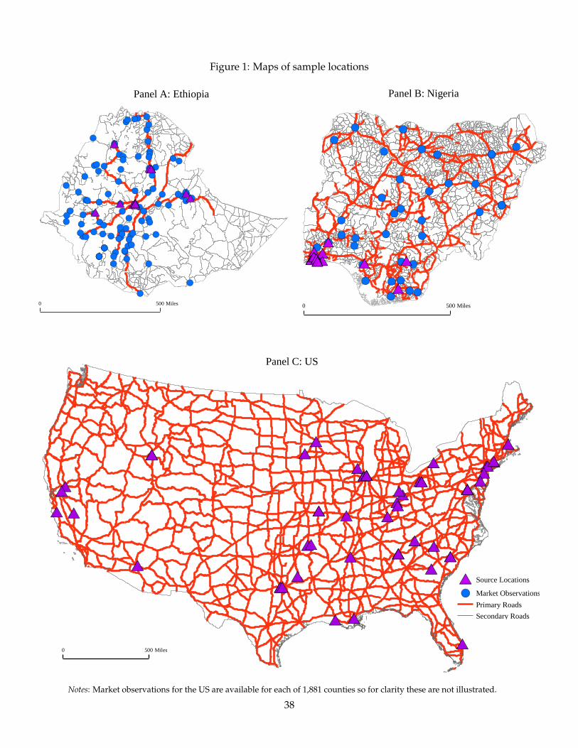
Figure 1: Maps of sample locations

Panel A: Ethiopia Panel B: Nigeria

Panel C: US

0 500 Miles

#*

#*

#*#*

#*#*

#*#*#*

#*#*

#*

#*

#*

#*

#*

#*

#*

#*#*

#*

#*

#*#*

#*#*

#*#*

#*#* #*#*#*#*

#*

#*

#*

#*

#*

#*

#*

#*#*

#*

#*#*

#*

#*

#*

#*

#*

#*

#*

#*

#*#*

0 500 Miles

!(

!(!(

!(

!(

!(

!(

!(!(

!(

!(

!(

!(

!(

!(

!(

!(!(

!(

!(!(

!( !(!(

!(

!(

!(

!(

!(

!(

!(

!(

!(

!(

!(

!(

!(!(

!(

!(

!(

!(

!(!(

!(

!(

!(

!(

!(

!(

!(

!(

!(

!(

!(!(

!(!(

!(

!(

!(

!(

!(

!(

!(

!(

!(

!(

!(

!(

!(

!(

!(

!(

!(

!(

!(

!(

!(

!(

!(

!(

!(

!(

!(

!(

!(

!(

!(

!( !(!(

!( !(!(

!(

!(

!(

!(

!(

!(

#*

#*#*

#*#*

#*#*

#*#*

#* #*#*#*#*

#*

#*#*

#*

0 500 Miles

!(

!( !(

!(

!(

!(

!(

!(

!(

!(!(

!(!(

!(

!(

!(

!(

!(

!(

!(

!(

!(!(

!(

!(

!(

!(

!(

!( !(!(

!(

!(

!(

!(

!(

!(!(

#*#*#*#*#*#*#*#*#*#* #*

#*

#*#*#*#*#*#*#*#*

#*

#* Source Locations

!( Market Observations

Primary Roads

Secondary Roads

Notes: Market observations for the US are available for each of 1,881 counties so for clarity these are not illustrated.

38

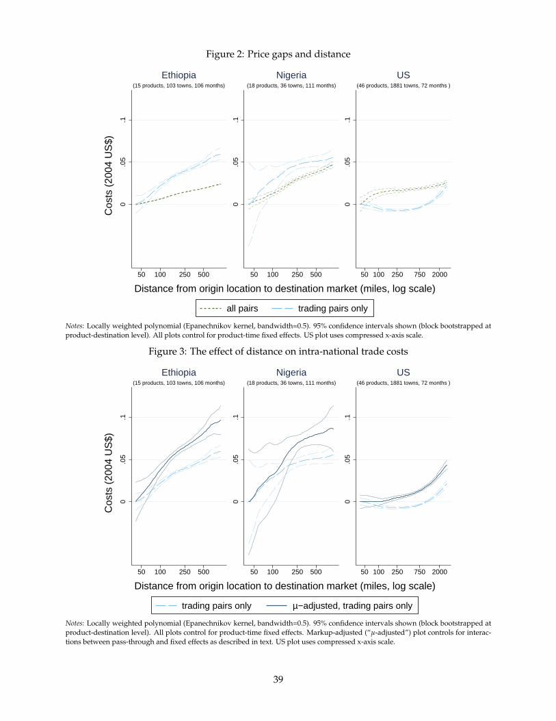
Figure 2: Price gaps and distance

0.0

5.1

50 100 250 500

(15 products, 103 towns, 106 months)

Ethiopia

0.0

5.1

50 100 250 500

(18 products, 36 towns, 111 months)

Nigeria

0.0

5.1

50 100 250 750 2000

(46 products, 1881 towns, 72 months )

US

Cos

ts (

2004

US

$)

Distance from origin location to destination market (miles, log scale)

all pairs trading pairs only

Notes: Locally weighted polynomial (Epanechnikov kernel, bandwidth=0.5). 95% confidence intervals shown (block bootstrapped atproduct-destination level). All plots control for product-time fixed effects. US plot uses compressed x-axis scale.

Figure 3: The effect of distance on intra-national trade costs

0.0

5.1

50 100 250 500

(15 products, 103 towns, 106 months)

Ethiopia

0.0

5.1

50 100 250 500

(18 products, 36 towns, 111 months)

Nigeria

0.0

5.1

50 100 250 750 2000

(46 products, 1881 towns, 72 months )

US

Cos

ts (

2004

US

$)

Distance from origin location to destination market (miles, log scale)

trading pairs only µ−adjusted, trading pairs only

Notes: Locally weighted polynomial (Epanechnikov kernel, bandwidth=0.5). 95% confidence intervals shown (block bootstrapped atproduct-destination level). All plots control for product-time fixed effects. Markup-adjusted (“µ-adjusted”) plot controls for interac-tions between pass-through and fixed effects as described in text. US plot uses compressed x-axis scale.

39

Figure 4: Variation in mark-ups across space

−.1

0.1

50 100 250 500

(15 products, 103 towns, 106 months)

Ethiopia

−.1

0.1

50 100 250 500

(18 products, 36 towns, 111 months)

Nigeria

−.1

0.1

50 100 250 750 2000

(46 products, 1881 towns, 72 months )

US

Cos

ts (

2004

US

$)

Distance from origin location to destination market (miles, log scale)

µ(x) −τ(x) a(x)

Notes: Locally weighted polynomial (Epanechnikov kernel, bandwidth=0.5). Semiparametric plots of demand shifters and trade costsfrom the adjusted price gap regression (i.e. equation 15). US plot uses compressed x-axis scale.

Figure 5: Product availability

.75

.8.8

5.9

.95

50 100 250 500

Ethiopia

.75

.8.8

5.9

.95

50 100 250 500

Nigeria

Pro

duct

Fou

nd b

y E

num

erat

ors

(Bin

ary)

Distance from origin location to destination market (miles, log scale)

Notes: Locally weighted polynomial (Epanechnikov kernel, bandwidth=0.5). 95% confidence intervals shown. Linear probabilitymodel. Sample restricted to time-product pairs where product found in at least one location.

40

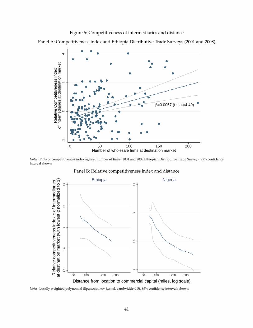
Figure 6: Competitiveness of intermediaries and distance

Panel A: Competitiveness index and Ethiopia Distributive Trade Surveys (2001 and 2008)

b=0.0057 (t-stat=4.49)

12

34

Rel

ativ

e C

ompe

titiv

enes

s In

dex

of in

term

edia

ries

at d

estin

atio

n m

arke

t

0 50 100 150 200Number of wholesale firms at destination market

Notes: Plots of competitiveness index against number of firms (2001 and 2008 Ethiopian Distributive Trade Survey). 95% confidenceinterval shown.

Panel B: Relative competitiveness index and distance

1.6

1.8

22.

22.

4

50 100 250 500

Ethiopia

22.

53

3.5

50 100 250 500

Nigeria

Rel

ativ

e co

mpe

titiv

enes

s in

dex

φ of

inte

rmed

iarie

sat

des

tinat

ion

mar

ket (

with

low

est φ

nor

mal

ized

to 1

)

Distance from location to commercial capital (miles, log scale)

Notes: Locally weighted polynomial (Epanechnikov kernel, bandwidth=0.5). 95% confidence intervals shown.

41

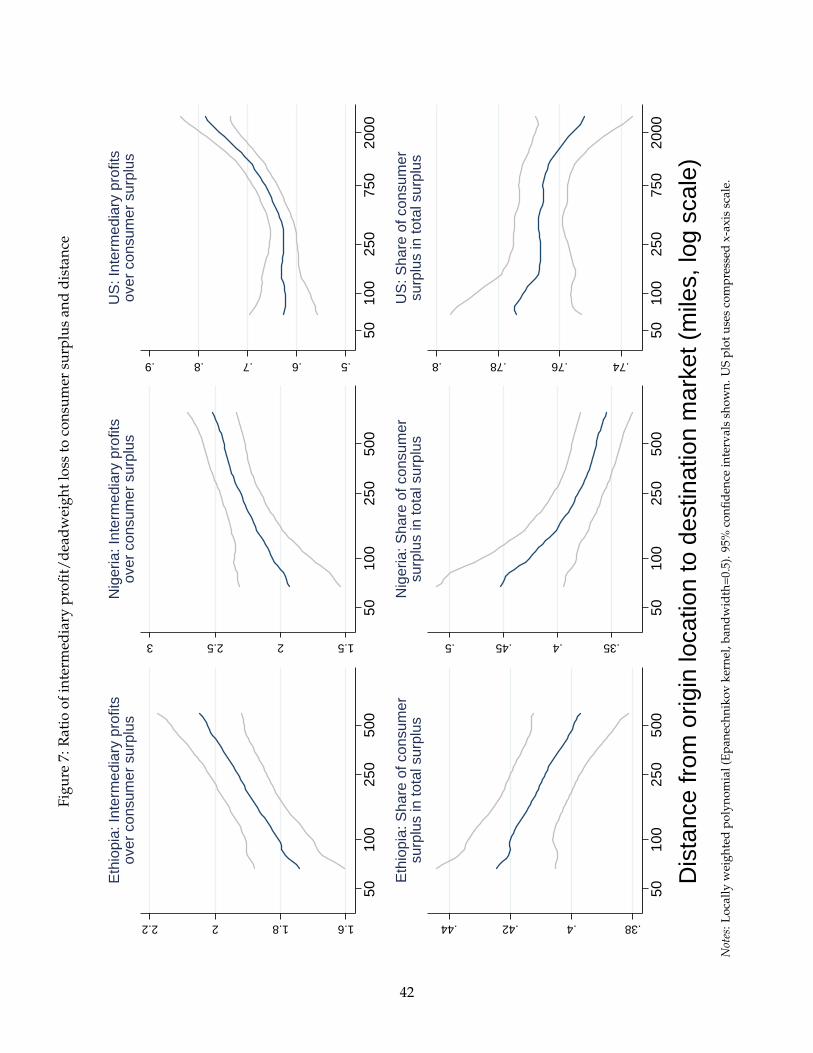
Figu

re7:

Rat

ioof

inte

rmed

iary

profi

t/de

adw

eigh

tlos

sto

cons

umer

surp

lus

and

dist

ance

1.61.822.2

5010

025

050

0

Eth

iopi

a: In

term

edia

ry p

rofit

sov

er c

onsu

mer

sur

plus

1.522.53

5010

025

050

0

Nig

eria

: Int

erm

edia

ry p

rofit

sov

er c

onsu

mer

sur

plus

.5.6.7.8.9

5010

025

075

020

00

US

: Int

erm

edia

ry p

rofit

sov

er c

onsu

mer

sur

plus

.38.4.42.44

5010

025

050

0

Eth

iopi

a: S

hare

of c

onsu

mer

surp

lus

in to

tal s

urpl

us.35.4.45.5

5010

025

050

0

Nig

eria

: Sha

re o

f con

sum

ersu

rplu

s in

tota

l sur

plus

.74.76.78.8

5010

025

075

020

00

US

: Sha

re o

f con

sum

ersu

rplu

s in

tota

l sur

plus

Dis

tanc

e fr

om o

rigin

loca

tion

to d

estin

atio

n m

arke

t (m

iles,

log

scal

e)N

otes

:Loc

ally

wei

ghte

dpo

lyno

mia

l(Ep

anec

hnik

ovke

rnel

,ban

dwid

th=0

.5).

95%

confi

denc

ein

terv

als

show

n.U

Spl

otus

esco

mpr

esse

dx-

axis

scal

e.

42

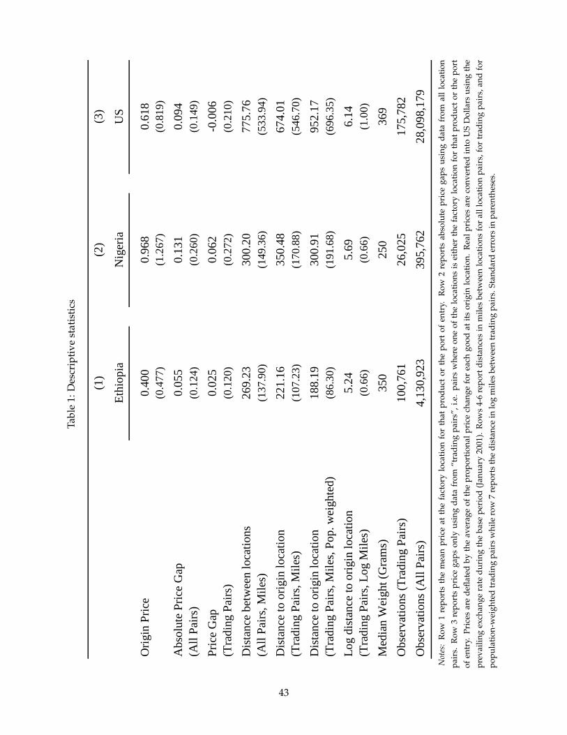
Tabl

e1:

Des

crip

tive

stat

isti

cs

(1)

(2)

(3)

Ethi

opia

Nig

eria

US

Orig

in P

rice

0.40

00.

968

0.61

8(0

.477

)(1

.267

)(0

.819

)

Abs

olut

e Pr

ice

Gap

0.05

50.

131

0.09

4(A

ll Pa

irs)

(0.1

24)

(0.2

60)

(0.1

49)

Pric

e G

ap0.

025

0.06

2-0

.006

(Tra

ding

Pai

rs)

(0.1

20)

(0.2

72)

(0.2

10)

Dis

tanc

e be

twee

n lo

catio

ns26

9.23

300.

2077

5.76

(All

Pairs

, Mile

s)(1

37.9

0)(1

49.3

6)(5

33.9

4)

Dis

tanc

e to

orig

in lo

catio

n22

1.16

350.

4867

4.01

(Tra

ding

Pai

rs, M

iles)

(107

.23)

(170

.88)

(546

.70)

Dis

tanc

e to

orig

in lo

catio

n18

8.19

300.

9195

2.17

(Tra

ding

Pai

rs, M

iles,

Pop.

wei

ghte

d)(8

6.30

)(1

91.6

8)(6

96.3

5)

Log

dist

ance

to o

rigin

loca

tion

5.24

5.69

6.14

(Tra

ding

Pai

rs, L

og M

iles)

(0.6

6)(0

.66)

(1.0

0)

Med

ian

Wei

ght (

Gra

ms)

350

250

369

Obs

erva

tions

(Tra

ding

Pai

rs)

100,

761

26,0

2517

5,78

2O

bser

vatio

ns (A

ll Pa

irs)

4,13

0,92

339

5,76

228

,098

,179

Not

es:

Row

1re

port

sth

em

ean

pric

eat

the

fact

ory

loca

tion

for

that

prod

uct

orth

epo

rtof

entr

y.R

ow2

repo

rts

abso

lute

pric

ega

psus

ing

data

from

all

loca

tion

pair

s.R

ow3

repo

rts

pric

ega

pson

lyus

ing

data

from

“tra

ding

pair

s”,i

.e.

pair

sw

here

one

ofth

elo

cati

ons

isei

ther

the

fact

ory

loca

tion

for

that

prod

uct

orth

epo

rtof

entr

y.Pr

ices

are

defla

ted

byth

eav

erag

eof

the

prop

orti

onal

pric

ech

ange

for

each

good

atit

sor

igin

loca

tion

.R

ealp

rice

sar

eco

nver

ted

into

US

Dol

lars

usin

gth

epr

evai

ling

exch

ange

rate

duri

ngth

eba

sepe

riod

(Jan

uary

2001

).R

ows

4-6

repo

rtdi

stan

ces

inm

iles

betw

een

loca

tion

sfo

ral

lloc

atio

npa

irs,

for

trad

ing

pair

s,an

dfo

rpo

pula

tion

-wei

ghte

dtr

adin

gpa

irs

whi

lero

w7

repo

rts

the

dist

ance

inlo

gm

iles

betw

een

trad

ing

pair

s.St

anda

rder

rors

inpa

rent

hese

s.

43

Table 2: Estimating the effect of distance on intra-national trade costs

Dependent variable: Absolute Price Gap(All Pairs)

Price Gap(Trading Pairs)

Adjusted Price Gap(Trading Pairs)

(1) (2) (3)

Log distance to origin (miles) 0.0115*** 0.0248*** 0.0374***(0.000439) (0.00125) (0.00223)

{0.00370}[0.00594]

Observations 4,130,923 100,761 100,761R-squared 0.356 0.252 0.932

(4) (5) (6)

Log distance to origin (miles) 0.0210*** 0.0254*** 0.0558***(0.00237) (0.00437) (0.00759)

{0.0115}[0.0221]

Observations 395,762 26,025 26,025R-squared 0.500 0.500 0.964

(7) (8) (9)

Log distance to origin (miles) 0.00684*** 0.00437*** 0.0106***(0.000480) (0.000731) (0.00100)

{0.00142}[0.00140]

Observations 28,098,179 175,782 175,782R-squared 0.432 0.408 0.928

Time-Product FE Yes Yes Yes

Time-Product No No Yes

Destination No No Yes

Nigeria

US

Ethiopia

×1 − �𝜌𝜌�𝜌𝜌

×1 − �𝜌𝜌�𝜌𝜌

×1 − �𝜌𝜌�𝜌𝜌

×1 − �𝜌𝜌�𝜌𝜌

Notes: Columns 1, 4 and 7 use data on the absolute price gap between all location pairs. Columns 2, 5 and 8 use dataon the actual price gap between “trading pairs”, e.g. destination price minus origin price for pairs where one of thelocations is either the factory location for that product or the port of entry. Columns 3, 6 and 9 use the adjusted price gap(Pk

dt − ρ̂kodPk

ot)/ρ̂kod and additionally include time-product and destination fixed effects multiplied by (1− ρ̂k

od)/ρ̂kod in

order to control for omitted variable bias due to the level of market power covarying with distance. Prices are deflatedby the average of the proportional price change for each good at its origin location. Real prices are converted into USDollars using the prevailing exchange rate during the base period (January 2001). All regressions include time-productfixed effects. Time-product clustered standard errors in round parentheses. Time-product block bootstrapped standarderrors in curly parentheses, product-destination block bootstrapped standard errors in square parentheses. * significantat 10 percent level, ** at 5 percent and *** at 1 percent.

44

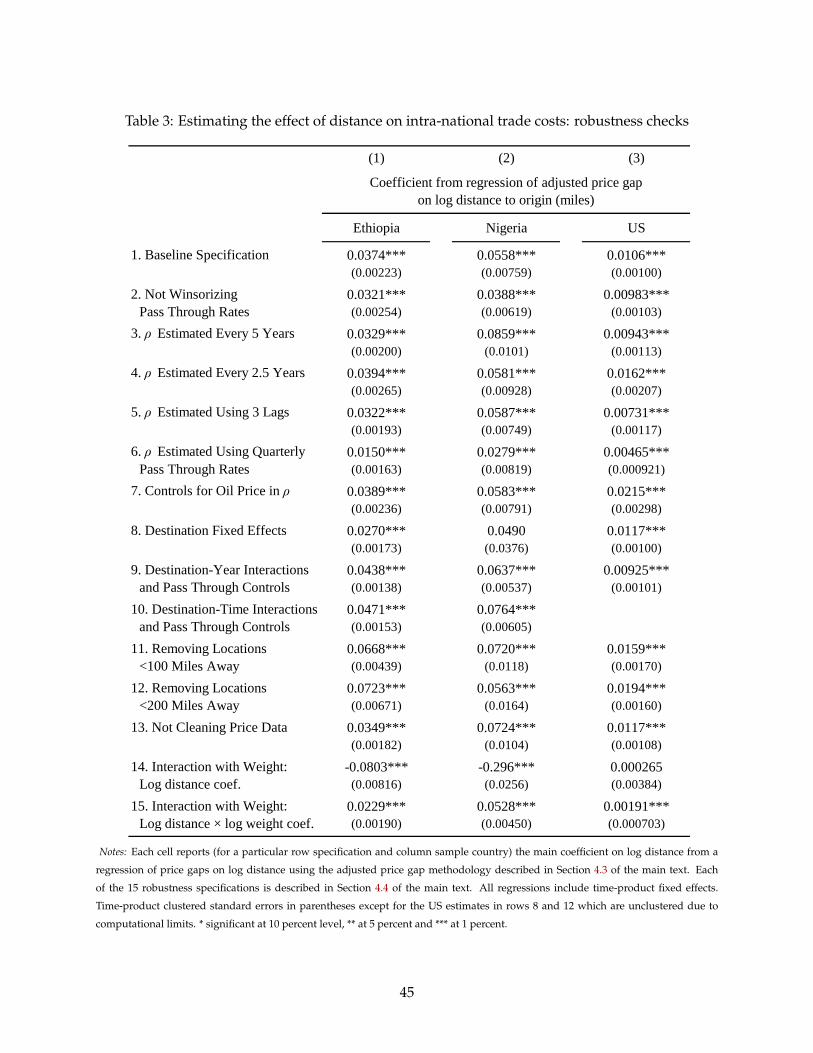
Table 3: Estimating the effect of distance on intra-national trade costs: robustness checks

(1) (2) (3)

Ethiopia Nigeria US

1. Baseline Specification 0.0374*** 0.0558*** 0.0106***(0.00223) (0.00759) (0.00100)

2. Not Winsorizing 0.0321*** 0.0388*** 0.00983***Pass Through Rates (0.00254) (0.00619) (0.00103)

3. ρ Estimated Every 5 Years 0.0329*** 0.0859*** 0.00943***(0.00200) (0.0101) (0.00113)

4. ρ Estimated Every 2.5 Years 0.0394*** 0.0581*** 0.0162***(0.00265) (0.00928) (0.00207)

5. ρ Estimated Using 3 Lags 0.0322*** 0.0587*** 0.00731***(0.00193) (0.00749) (0.00117)

6. ρ Estimated Using Quarterly 0.0150*** 0.0279*** 0.00465***Pass Through Rates (0.00163) (0.00819) (0.000921)

7. Controls for Oil Price in ρ 0.0389*** 0.0583*** 0.0215***(0.00236) (0.00791) (0.00298)

8. Destination Fixed Effects 0.0270*** 0.0490 0.0117***(0.00173) (0.0376) (0.00100)

9. Destination-Year Interactions 0.0438*** 0.0637*** 0.00925***and Pass Through Controls (0.00138) (0.00537) (0.00101)

10. Destination-Time Interactions 0.0471*** 0.0764***and Pass Through Controls (0.00153) (0.00605)

11. Removing Locations 0.0668*** 0.0720*** 0.0159***<100 Miles Away (0.00439) (0.0118) (0.00170)

12. Removing Locations 0.0723*** 0.0563*** 0.0194***<200 Miles Away (0.00671) (0.0164) (0.00160)

13. Not Cleaning Price Data 0.0349*** 0.0724*** 0.0117***(0.00182) (0.0104) (0.00108)

14. Interaction with Weight: -0.0803*** -0.296*** 0.000265Log distance coef. (0.00816) (0.0256) (0.00384)

15. Interaction with Weight: 0.0229*** 0.0528*** 0.00191***Log distance × log weight coef. (0.00190) (0.00450) (0.000703)

Coefficient from regression of adjusted price gapon log distance to origin (miles)

Notes: Each cell reports (for a particular row specification and column sample country) the main coefficient on log distance from a

regression of price gaps on log distance using the adjusted price gap methodology described in Section 4.3 of the main text. Each

of the 15 robustness specifications is described in Section 4.4 of the main text. All regressions include time-product fixed effects.

Time-product clustered standard errors in parentheses except for the US estimates in rows 8 and 12 which are unclustered due to

computational limits. * significant at 10 percent level, ** at 5 percent and *** at 1 percent.

45

Table 4: Comparisons across distance metrics and existing estimates

(1) (2)

Ethiopia Nigeria

Great circle distance 3.53 5.26

Road distance 3.19 5.40

Travel time 2.46 4.01

(3) (4)

East Africa

(Mombasa-Nairobi)

West Africa

(Bamako-Accra)

Per km for one truckload 1.88 3.28

Ratio relative to US trucking costs

Ratio relative to US marginal cost of distance

Notes: Columns 1 and 2 report the ratio of the coefficient on log distance for Ethiopia and Nigeria respectively, eachcompared to the coefficient on log distance for the US, from regressions of the adjusted price gap (Pk

dt − ρ̂kodPk

ot)/ρ̂kod on

log distance and time-product and destination fixed effects multiplied by (1− ρ̂kod)/ρ̂k

od in order to control for omittedvariable bias due to the level of market power covarying with distance. Ratios are presented for estimates calculatedusing three different distance metrics: row 1 uses geodesic (i.e. as the crow flies) distance, row 2 uses quickest routeroad distance as calculated by Google Maps, and row 3 uses quickest route travel time again calculated by GoogleMaps. The raw coefficients on log distance using these alternate distance metrics are reported in Appendix Table C.2.Columns 3 and 4 report ratios of trucking costs along major East and West African transport corridors relative to UStrucking costs from Teravaninthorn and Raballand (2009) (all calculated per km for one truckload through surveys oftrucking firms).

46

Table 5: Regressing product availability, competitiveness and surplus on distance

(1) (2) (3) (4) (5)

Dependent variable:

y1=Price Record,

0=No Price Record(Time-Good-

Location)

CompetitivenessIndex of

Intermediaries(All Locations)

Ratio of Intermediary Profits

to Consumer Surplus(Good-Location)

Ratio of Deadweight Loss toConsumer Surplus(Good-Location)

Consumer's Shareof Total Surplus

(Good-Location)

Log distance between -0.0959*** 0.229*** 0.0368*** -0.0185**origin and destination (0.00309) (0.0598) (0.00908) (0.00763)

Log distance between -0.344***location and Addis Ababa (0.127)

Observations 145,682 100 1,418 1,418 1,418R-squared 0.14 0.059 0.009 0.009 0.004

(6) (7) (8) (9) (10)

Dependent variable:

y1=Price Record,

0=No Price Record(Time-Good-

Location)

CompetitivenessIndex of

Intermediaries(All Locations)

Ratio of Intermediary Profits

to Consumer Surplus(Good-Location)

Ratio of Deadweight Loss toConsumer Surplus(Good-Location)

Consumer's Shareof Total Surplus

(Good-Location)

Log distance between -0.0490*** 0.347*** 0.0833*** -0.0546***origin and destination (0.00410) (0.113) (0.0138) (0.0155)

Log distance between -0.444***location and Lagos (0.114)

Observations 35,406 36 526 526 526R-squared 0.298 0.168 0.019 0.063 0.023

(11) (12) (13) (14)

Dependent variable:

CompetitivenessIndex of

Intermediaries(All Locations)

Ratio of Intermediary Profits

to Consumer Surplus(Good-Location)

Ratio of Deadweight Loss toConsumer Surplus(Good-Location)

Consumer's Shareof Total Surplus

(Good-Location)

Log distance between 0.0623*** -0.000350 -0.00422origin and destination (0.0108) (0.000299) (0.00372)

Log distance between 25.33location and Chicago (54.71)

Observations 2,865 9,614 9,564 9,564R-squared 0.000 0.003 0.000 0.000

Ethiopia

Nigeria

US

Notes: Columns 1 and 6 regress product availability on log distance at the monthly time-product-location level by ordinary least

squares. Sample restricted to monthly time-product pairs for which the product is observed in at least one location. Both columns

include time-product fixed effects and time-product clustered standard errors are reported in parentheses. Columns 2 to 5, 7 to 10 and

11 to 14 regress estimates of the competitiveness index, the ratio of intermediary profit to consumer surplus, the ratio of deadweight

loss to consumer surplus and the share of consumer surplus in total surplus on log distance. Since the competitiveness index is

location not location-product specific, distance to the commercial capital is used in columns 2, 7 and 11 rather than origin-destination

distance. Standard errors in parentheses. * significant at 10 percent level, ** at 5 percent and *** at 1 percent.

47

A Data AppendixThe methodology proposed in the main text requires retail price data for narrowly defined

products, at many points in space within a group of developing and developed countries, at highfrequency for many periods. Here we supplement Section 2 with a more detailed description ofthe data sources we use to obtain these price data and how we construct our retail price dataset.(In the interest of readability and completeness, we repeat certain details that are also containedin the main text.) We apply our methodology to a sample from two sub-Saharan African coun-tries (Ethiopia and Nigeria) and from the United States. The construction of our African and USsamples differ, so we describe them separately below.

A.1 Ethiopia and Nigeria

Because particularly little is known about the magnitude and implications of intra-nationaltrade costs in sub-Saharan Africa (SSA), we began the data collection exercise underpinning thispaper with a search for SSA countries that collect high quality retail price data satisfying the fol-lowing requirements. First, a substantial number of sampled products must be extremely nar-rowly defined (that is, defined at a level equivalent to the barcode level). Second, the price ofthese products prevailing at retail markets must be recorded at many locations throughout thecountry. And finally, these price records must be recorded at high frequency (e.g. on a monthlybasis) and for at least six years (the length of our US sample, as described below). While the of-ficial data collection infrastructure in this region is generally weak (Young, 2012), it is relativelystrong for the purposes of collecting the official consumer price index via surveys of the prices ofproducts at retail establishments. Fortunately, therefore, many SSA countries (and developing anddeveloped countries more widely) collect exactly the type of data that is required for our analysis.We work with two SSA countries in particular—Ethiopia and Nigeria—because of their large ge-ographic sizes and because they were particularly forthcoming in making available to researchersmicrodata on unit-level CPI observations. We obtained data in digital form spanning the periodfrom September 2001 to June 2010 in the case of Ethiopia and January 2001 to July 2010 in the caseof Nigeria.

Selection of Locations: Both Ethiopia and Nigeria report a CPI that is based on price observa-tions in urban areas. In Ethiopia we obtained a sample of 103 urban market places1 and in Nigeriawe obtained a sample of 36 state capitals (one for each state).2 These locations are shown on themaps of Ethiopia and Nigeria depicted in panels A and B of Figure 1 of the main text, respectively.Reassuringly, the sample locations provide fairly even geographic coverage of these two countries.

Survey Procedure: Enumerators visit pre-specified sample outlet locations within a market townor city, typically many times per month.3 They are instructed to find the precise product described

1Urban market places are defined as localities with 2,000 or more inhabitants with exceptions made for administra-tive capitals. The urban market places in the survey were chosen to be nationally representative and were either a cap-ital of an administrative region, an industrial market place and/or a market place for trade and commercial activities.

2For larger states in Nigeria, our price observations are actually an average of prices in the state capital and othermajor cities within the state as discussed further in footnote 5, below.

3In Ethiopia, prices are surveyed every day for the first fifteen days of the month; whereas in Nigeria, most of the

1

in each product’s description and to report a missing value if that product was unavailable (that is,substitutes are not permitted). Once found, the enumerator’s job is to learn at what price the prod-uct would typically be sold on the given date and at the given location.4 The sample frame of out-lets is intended to comprise a representative sample of open markets, kiosks, groceries, butcheries,pharmacies, super markets, etc.. In many cases, multiple outlet observations are obtained.5

Selection of Products: Both Ethiopia and Nigeria base their CPI on a set of products that did notsubstantially change during our sample period of 2001-2010. These products are designed to spanthe typical consumption basket (among both goods and services) in each country. Of the manyproducts that are covered, the vast majority refer to activities—such as a “man’s haircut” or a “onekm taxi journey”—or goods—such as “rice” or “bread”—whose very nature means that the prod-ucts cannot be precisely codified. To avoid concerns of spatially-varying unobserved quality dif-ferences we work with the sub-sample of products that we consider to be “narrowly defined.” Inpractice, this involved a restriction to products whose producer’s brandname was provided in theproduct description. Most products for which a brandname was provided contained additionaldetails, such as a description including the product size, which were designed to be sufficientlyprecise to allow enumerators to locate the exact product.6 Because these descriptions appear to beas precise as those linked to unique barcodes in the US Nielsen Consumer Panel data describedbelow, we refer to these products as products that are defined at the “barcode level.” The resultingsample contains 15 products in Ethiopia and 19 products in Nigeria that were broadly availableacross both the locations and years in our sample (examples of which include “Titus Sardines”(125gm), “Bedele Beer” (300cc) and “Lux Toilet Soap” (90gm)).

Additional Processing: As with all micro-level price data, our data contain observations thatappear to be mis-recorded.7 Accordingly, our main analysis uses a cleaned sample of price data,obtained by applying a simple cleaning algorithm to the raw data.8 However, we also report (in

products in our sample are surveyed once per week throughout the entire month. In both cases, the data available tous are an average over these multiple temporal observations per month.

4The precise means by which these instructions are conveyed to enumerators varies across the two countries. InEthiopia, enumerators do not actually purchase the items in question but instead interview traders and consumersabout prices typically paid (after bargaining). In Nigeria, enumerators are instructed to make actual (bargained)purchases where thought necessary. The Nigerian enumerators’ manual advises that the enumerator “must not be toosophisticated in dressing as this may make the respondent arbitrarily raise the price of his goods”.

5In Ethiopia, price observations are collected at 1-3 outlets per location, with the exception of three larger cities(Addis Ababa, Dire Dawa and Harar) in which case the city is first divided into a number of separate major marketareas and then 1-3 outlets are surveyed per market area. In Nigeria, two outlets are selected in each state capital, andalso in each of up to two other urban locations within the state; the precise locations of these non-capital locationschange from from month to month and are not known to us so we therefore take the location to be simply the statecapital’s location. The data available to us comprise an average over these multiple spatial observations per date.

6Exceptions were the “Singer sewing machine” and the “Philips electric iron” in Nigeria; and the “National taperecorder (2 speaker)”, the “Croft Men’s Leather Shoes”, the “Philips 3 band Radio” and the “Philips 21 inch color TV”in Ethiopia. We drop these products because their descriptions do not appear to be precise enough to determine theexact product being surveyed.

7In the majority of these cases it appears that the enumerator in a particular location obtained the price for adifferent size or specification of product (contrary to instructions). While any such substitutions are meant to berecorded and flagged by enumerators to avoid such errors, we conjecture that such information was lost in thereporting and digitization process.

8The algorithm is as follows. First, we remove price quotes that lie more than 10 standard deviations away fromthe log mean price of a product. Second, we eyeball the time series of prices for each product in each location. If a price

2

Table 3 of the main text) results obtained from the original, uncleaned data set; these are similarin terms of both the magnitudes and statistical significance of the estimates. In addition, in orderto arrive at estimates of trade costs that are in real terms, we require all prices to be similarly ex-pressed in terms that correspond to a common year (which we take to be 2001) and a commoncurrency unit (US dollars). We therefore apply a simple procedure to correct for inflation, basedon prices at origin locations, and then further convert all prices used in the analysis into 2001 USdollars using the prevailing exchange rate at that time.9

A.2 United States

In order to provide a basis of comparison for our Ethiopian and Nigerian estimates, we seeksimilar estimates for the United States. Following Broda and Weinstein (2008), we use data fromthe Nielsen Consumer Panel (NCP, formerly known as the AC Nielsen Homescan ConsumerPanel) due to its extensive geographic and product coverage.10 We have access to data span-ning the period from January 2004 to December 2009. The NCP incentivizes sample households(of which there were approximately 40,000 between 2004 and 2007 and 60,000 in the last two yearsof our sample) to use hand-held barcode scanners, at home, to scan all products purchased bythe household on the date of purchase and, where necessary (that is, when a purchase is made ata smaller retail establishment that does not participate in Nielsen’s “ScanTrak” system), enter theprice that they paid for each product purchased. From the resulting price observations over space,products and time (of which there are over 300 million) we use each household’s county of resi-dence to aggregate up to a dataset that contains the average price paid, in each of the 2,856 countiesand each month in 2004-2009, for the 1.4 million unique barcodes purchased by NCP households.

Unlike the samples for Ethiopia and Nigeria which are collected in order to calculate the CPI,the NCP includes many products that are neither widely available across the US nor importantcomponents of the average household budget. In order to obtain a sample similar in nature tothe SSA samples, we work with relatively small sub-sample of barcodes that are the leading prod-uct in each of Nielsen’s 230 “product modules” (examples of which include frozen pot pies, chilisauce, or women’s shaving cream).11

quote seems unusually high or low, we verify whether nearby prices for that same product in that same period werealso unusually high. If they were not, we remove this outlier.

9This procedure is as follows. For every origin location-product-month price observation used in our analysis, wecalculate the proportional change in price over the previous month. We then calculate the (unweighted) mean of allthese proportional price changes across all products in our sample for each month and use this as a measure of monthlyinflation relative to the previous month with which to convert all prices into real prices in the base period. In the rarecase when a product price is not observed at the source location in a given month we use the pro-rated multi-monthchange between available monthly observations. The normalized prices are converted into 2001 US dollars using theprevailing exchange rate during the first month of the sample.

10We obtained the NCP data from the Kilts-Nielsen Data Center at The University of Chicago Booth School ofBusiness (http://research.chicagobooth.edu/nielsen).

11We define the leading product as the barcode that is represented in the greatest number of counties per year,averaged across 2004-2009. In order to maximize spatial and temporal coverage, we omit certain barcodes (thoseobserved in fewer than 100 counties per year in each sample year, or in fewer than four years) prior to calculating theleading barcode. . We also omit barcodes of supermarket own-brand items since the NCP anonymizes the supermarketname for confidentiality reasons hence these barcodes do not uniquely identify a particular product. After theseomissions, 230 product categories contained at least one barcode.

3

B Theoretical AppendixIn this appendix we formally prove the claim in equation (16) that the share of surplus enjoyed,

in equilibrium, by intermediaries relative to consumers is a simple function of just the equilibriumpass-through rate ρd and the competitiveness index φd prevailing in that market. We revert to thenotation of Section 3 here, considering just one product in one time period in one destination d.

Consider first the calculation of the amount of consumer surplus generated by the presenceof the product in destination market d in any partial equilibrium market setting (that is, wherethe prices in all other markets are held constant). Consumer surplus when Qd is supplied to themarket is defined as CSd(Qd) ≡

∫ Qdψ=0[Pd(ψ)− Pd(Qd)]dψ, where Pd(ψ) is the consumers’ inverse

demand curve evaluated at quantity ψ and Qd is the total amount consumed in equilibrium in themarket. Now consider a marginal change in the exogenous origin price, Po. The marginal changein consumer surplus is then, by an envelope argument, dCSd(Qd)

dPo= −Qd(Pd(Po))ρd(Po), where, in

a slight abuse of notation, Qd(Pd(Po)) indicates that the quantity consumed depends on the desti-nation price Pd, but the destination price is itself a function of the level of the origin price: Pd(Po).Similarly, ρd(Po) is the equilibrium pass-through rate when the origin price is Po. Integrating suchsmall changes from the original value of the origin price, Po, to the highest value the origin pricecan take, infinity, the total consumer surplus available in this market (whose origin price is Po) is:

CSd(Po) =∫ ∞

υ=Po

Qd(Pd(υ))ρd(υ)dυ. (19)

This is an alternative expression for the level of consumer surplus in the market that highlights itsessential connection to the pass-through rate.

We now seek a similar expression for the amount of intermediaries’ surplus in this market,ISd(Po). The equilibrium level of profits for one intermediary is Πd(Qd) = [Pd(Qd)− Po − τ(Xd)].Differentiating this with respect to Po yields

dΠd(Qd)

dPo= [ρd(Po)− 1]qd + [Pd(Qd)− Po − τ(Xd)]

dQd

dPo

1md

(20)

in a symmetric equilibrium. Applying the chain rule to dQddPo

and noting that the intermediary’sfirst-order condition requires that Pd(Qd)− Po − τ(Xd) = − dPd

dQdθdqd we have

dΠd(Qd)

dPo= qd

[ρd(Po)

(φd − 1

φd

)− 1]

, (21)

where φd ≡ mdθd

is the ‘competitiveness index’ introduced in Section 3.1 of the main text. Integrat-ing these small changes to Po from its starting value, Po, to the highest value that it can take, andagain summing over the md symmetric intermediaries serving market d, the total intermediaries’surplus available in this market is:

ISd(Po) =∫ ∞

υ=Po

Qd(Pd(υ))dυ +

(1− φd

φd

) ∫ ∞

υ=Po

Qd(Pd(υ))ρd(υ)dυ. (22)

Applying equations (19) and (22) it is then straightforward to show that the ratio of interme-

4

diaries’ surplus ISd(Po) to consumer surplus CSd(Po) in the market at destination location d whenthe origin price is Po is given by

ISd

CSd(Po) =

1

(ρQ)d+

1− φd

φd, (23)

where (ρQ)d is a quantity weighted average of the pass-through rate, defined as

(ρQ)d ≡∫ ∞

υ=PoQd(Pd(υ))ρd(υ)dυ∫ ∞

υ=PoQd(Pd(υ))dυ

. (24)

The result in equation (23), which is derived for a completely general demand structure, high-lights the close connection between pass-through and the division of surplus in a general oligopolis-tic setting. However, pass-through enters this formula always as a weighted average (ρQ)d of pass-through values at different quantities. Unfortunately, in our setting the weights in this weightedaverage formula (consumption quantities Qd(Pd(υ)) are not observed, nor is there any hope ofcredibly estimating the demand structure so as to estimate these weights because consumptionquantities are not observed. However, in the case of the constant pass-through class of demand(i.e. that described in Assumption 3 of the main text), pass-through is constant across quantities(that is, ρd(υ) = ρd for all υ) and hence the weights in equation (24) need not be observed. That is,under Assumption 3 we have

ISd

CSd(Po) =

1ρd

+1− φd

φd, (25)

the expression in equation (16) of the main text.

5

C Additional Figures and Tables

6

Figu

reC

.1:T

hedi

stri

buti

onof

popu

lati

onac

ross

spac

e

01,000,0002,000,0003,000,000

5010

025

050

0

Eth

iopi

a: A

ll G

oods

02,000,0004,000,0006,000,0008,000,000

5010

025

050

0

Nig

eria

05,000,00010,000,000

5010

025

075

020

00

US

Destination market population (mid sample period)

Dis

tanc

e fr

om o

rigin

loca

tion

to d

estin

atio

n m

arke

t (m

iles,

log

scal

e)

Not

es:D

ista

nce

from

orig

inlo

cati

onpl

otte

dag

ains

tthe

popu

lati

onin

the

dest

inat

ion

loca

tion

for

ever

ypr

oduc

t-lo

cati

onpa

ir.U

Spl

otus

esco

mpr

esse

dx-

axis

scal

e.

7

Figu

reC

.2:E

stim

ated

pass

-thr

ough

rate

sfo

ral

lgoo

dsan

ddi

stan

ce

0.25.5.751

5010

025

050

0

Eth

iopi

a

0.25.5.751

5010

025

050

0

Nig

eria

0.25.5.751

5010

025

075

020

00

US

Pass−through rate

Dis

tanc

e fr

om o

rigin

loca

tion

to d

estin

atio

n m

arke

t (m

iles,

log

scal

e)

Not

es:

Each

dot

isan

esti

mat

edpa

ss-t

hrou

ghra

tefo

ra

prod

uct-

loca

tion

pair

ρ̂k od

.Th

eso

lidlin

epl

ots

alo

cally

wei

ghte

dpo

lyno

mia

l(E

pane

chni

kov

kern

el,b

and-

wid

th=0

.5)o

fthe

sein

divi

dual

pass

-thr

ough

rate

s.95

%co

nfide

nce

inte

rval

ssh

own.

US

plot

uses

com

pres

sed

x-ax

issc

ale.

8

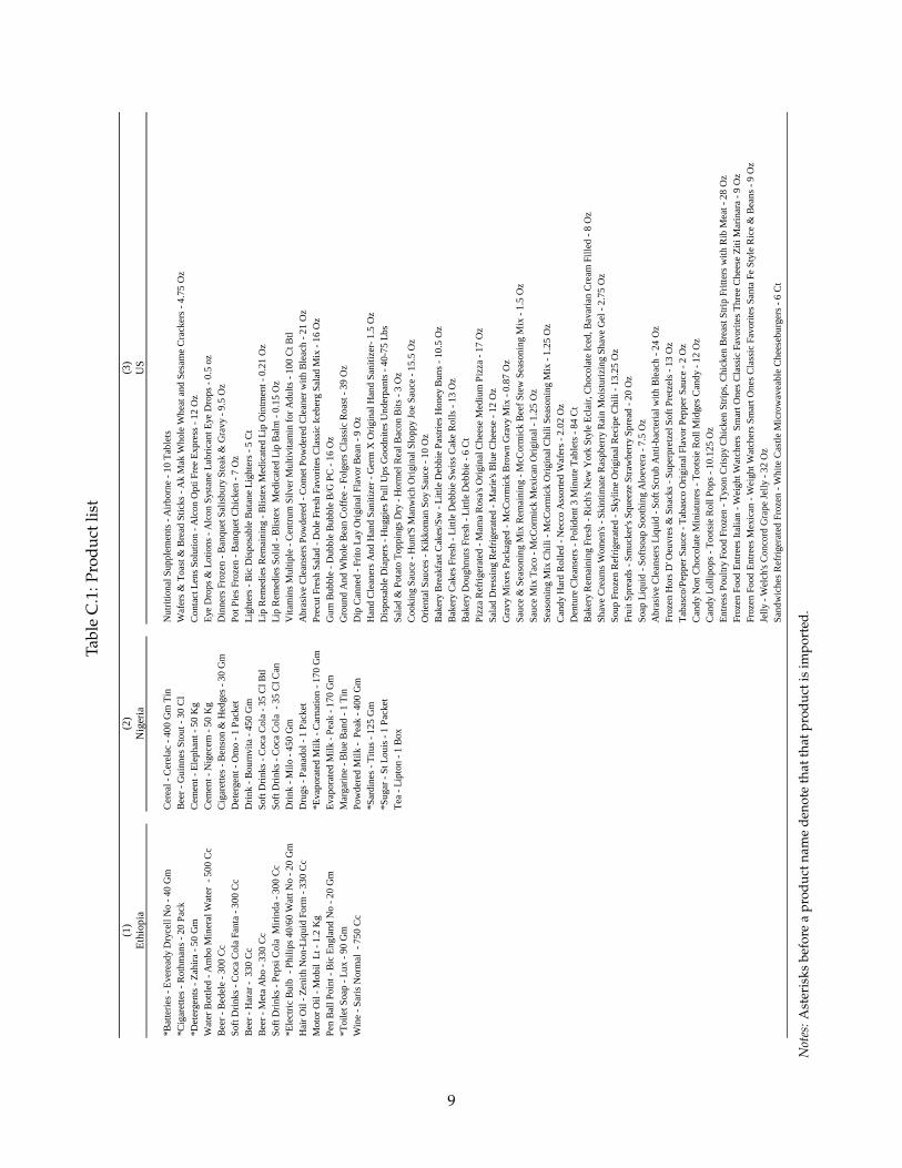
Tabl

eC

.1:P

rodu

ctlis

t

(1)

(2)

(3)

Ethi

opia

Nig

eria

US

*Bat

terie

s - E

vere

ady

Dry

cell

No

- 40

Gm

Cer

eal -

Cer

elac

- 40

0 G

m T

inN

utrit

iona

l Sup

plem

ents

- A

irbor

ne -

10 T

able

ts*C

igar

ette

s - R

othm

ans -

20

Pack

Beer

- G

uinn

es S

tout

- 30

Cl

Waf

ers &

Toa

st &

Bre

ad S

ticks

- A

k M

ak W

hole

Whe

at a

nd S

esam

e C

rack

ers -

4.7

5 O

z*D

eter

gent

s - Z

ahira

- 50

Gm

Cem

ent -

Ele

phan

t - 5

0 K

gC

onta

ct L

ens S

olut

ion

- Alc

on O

pti F

ree

Expr

ess -

12

Oz

Wat

er B

ottle

d - A

mbo

Min

eral

Wat

er -

500

Cc

Cem

ent -

Nig

ecem

- 50

Kg

Eye

Dro

ps &

Lot

ions

- A

lcon

Sys

tane

Lub

rican

t Eye

Dro

ps -

0.5

ozBe

er -

Bede

le -

300

Cc

Cig

aret

tes -

Ben

son

& H

edge

s - 3

0 G

mD

inne

rs F

roze

n - B

anqu

et S

alis

bury

Ste

ak &

Gra

vy -

9.5

Oz

Soft

Drin

ks -

Coc

a C

ola

Fant

a - 3

00 C

cD

eter

gent

- O

mo

- 1 P

acke

tPo

t Pie

s Fro

zen

- Ban

quet

Chi

cken

- 7

Oz

Beer

- H

arar

- 3

30 C

cD

rink

- Bou

rnvi

ta -

450

Gm

Ligh

ters

- Bi

c D

ispo

sabl

e Bu

tane

Lig

hter

s - 5

Ct

Beer

- M

eta

Abo

- 33

0 C

cSo

ft D

rinks

- C

oca

Col

a - 3

5 C

l Btl

Lip

Rem

edie

s Rem

aini

ng -

Blis

tex

Med

icat

ed L

ip O

intm

ent -

0.2

1 O

zSo

ft D

rinks

- Pe

psi C

ola

Miri

nda

- 300

Cc

Soft

Drin

ks -

Coc

a C

ola

- 35

Cl C

anLi

p R

emed

ies S

olid

- Bl

iste

x M

edic

ated

Lip

Bal

m -

0.15

Oz

*Ele

ctric

Bul

b -

Phili

ps 4

0/60

Wat

t No

- 20

Gm

Drin

k - M

ilo -

450

Gm

Vita

min

s Mul

tiple

- C

entru

m S

ilver

Mul

tivita

min

for A

dults

- 10

0 C

t Btl

Hai

r Oil

- Zen

ith N

on-L

iqui

d Fo

rm -

330

Cc

Dru

gs -

Pana

dol -

1 P

acke

tA

bras

ive

Cle

anse

rs P

owde

red

- Com

et P

owde

red

Cle

aner

with

Ble

ach

- 21

Oz

Mot

or O

il - M

obil

Lt -

1.2

Kg

*Eva

pora

ted

Milk

- C

arna

tion

- 170

Gm

Prec

ut F

resh

Sal

ad -

Dol

e Fr

esh

Favo

rites

Cla

ssic

Iceb

erg

Sala

d M

ix -

16 O

zPe

n Ba

ll Po

int -

Bic

Eng

land

No

- 20

Gm

Evap

orat

ed M

ilk -

Peak

- 17

0 G

mG

um B

ubbl

e - D

ubbl

e Bu

bble

B/G

PC

- 16

Oz

*Toi

let S

oap

- Lux

- 90

Gm

Mar

garin

e - B

lue

Band

- 1

Tin

Gro

und

And

Who

le B

ean

Cof

fee

- Fol

gers

Cla

ssic

Roa

st -

39 O

zW

ine

- Sar

is N

orm

al -

750

Cc

Pow

dere

d M

ilk -

Pea

k - 4

00 G

mD

ip C

anne

d - F

rito

Lay

Orig

inal

Fla

vor B

ean

- 9 O

z*S

ardi

nes -

Titu

s - 1

25 G

mH

and

Cle

aner

s And

Han

d Sa

nitiz

er -

Ger

m X

Orig

inal

Han

d Sa

nitiz

er- 1

.5 O

z*S

ugar

- St

Lou

is -

1 Pa

cket

Dis

posa

ble

Dia

pers

- H

uggi

es P

ull U

ps G

oodn

ites U

nder

pant

s - 4

0-75

Lbs

Tea

- Lip

ton

- 1 B

oxSa

lad

& P

otat

o To

ppin

gs D

ry -

Hor

mel

Rea

l Bac

on B

its -

3 O

zC

ooki

ng S

auce

- H

unt'S

Man

wic

h O

rigin

al S

lopp

y Jo

e Sa

uce

- 15.

5 O

zO

rient

al S

auce

s - K

ikko

man

Soy

Sau

ce -

10 O

zBa

kery

Bre

akfa

st C

akes

/Sw

- Li

ttle

Deb

bie

Past

ries H

oney

Bun

s - 1

0.5

Oz

Bake

ry C

akes

Fre

sh -

Littl

e D

ebbi

e Sw

iss C

ake

Rol

ls -

13 O

zBa

kery

Dou

ghnu

ts F

resh

- Li

ttle

Deb

bie

- 6 C

tPi

zza

Ref

riger

ated

- M

ama

Ros

a's O

rigin

al C

hees

e M

ediu

m P

izza

- 17

Oz

Sala

d D

ress

ing

Ref

riger

ated

- M

arie

's Bl

ue C

hees

e - 1

2 O

zG

ravy

Mix

es P

acka

ged

- McC

orm

ick

Brow

n G

ravy

Mix

- 0.

87 O

zSa

uce

& S

easo

ning

Mix

Rem

aini

ng -

McC

orm

ick

Beef

Ste

w S

easo

ning

Mix

- 1.

5 O

zSa

uce

Mix

Tac

o - M

cCor

mic

k M

exic

an O

rigin

al -

1.25

Oz

Seas

onin

g M

ix C

hili

- McC

orm

ick

Orig

inal

Chi

li Se

ason

ing

Mix

- 1.

25 O

zC

andy

Har

d R

olle

d - N

ecco

Ass

orte

d W

afer

s - 2

.02

Oz

Den

ture

Cle

anse

rs -

Polid

ent 3

Min

ute

Tabl

ets -

84

Ct

Bake

ry R

emai

ning

Fre

sh -

Ric

h's N

ew Y

ork

Styl

e Ec

lair,

Cho

cola

te Ic

ed, B

avar

ian

Cre

am F

illed

- 8

Oz

Shav

e C

ream

s Wom

en's

- Ski

ntim

ate

Ras

pber

ry R

ain

Moi

stur

izin

g Sh

ave

Gel

- 2.

75 O

zSo

up F

roze

n R

efrig

erat

ed -

Skyl

ine

Orig

inal

Rec

ipe

Chi

li - 1

3.25

Oz

Frui

t Spr

eads

- Sm

ucke

r's S

quee

ze S

traw

berry

Spr

ead

- 20

Oz

Soap

Liq

uid

- Sof

tsoa

p So

othi

ng A

loev

era

- 7.5

Oz

Abr

asiv

e C

lean

sers

Liq

uid

- Sof

t Scr

ub A

nti-b

acte

rial w

ith B

leac

h - 2

4 O

zFr

ozen

Hor

s D' O

euvr

es &

Sna

cks -

Sup

erpr

etze

l Sof

t Pre

tzel

s - 1

3 O

zTa

basc

o/Pe

pper

Sau

ce -

Taba

sco

Orig

inal

Fla

vor P

eppe

r Sau

ce -

2 O

zC

andy

Non

Cho

cola

te M

inia

ture

s - T

oots

ie R

oll M

idge

s Can

dy -

12 O

zC

andy

Lol

lipop

s - T

oots

ie R

oll P

ops -

10.

125

Oz

Entre

ss P

oultr

y Fo

od F

roze

n - T

yson

Cris

py C

hick

en S

trips

, Chi

cken

Bre

ast S

trip

Fritt

ers w

ith R

ib M

eat -

28

Oz

Froz

en F

ood

Entre

es It

alia

n - W

eigh

t Wat

cher

s Sm

art O

nes C

lass

ic F

avor

ites T

hree

Che

ese

Ziti

Mar

inar

a - 9

Oz

Froz

en F

ood

Entre

es M

exic

an -

Wei

ght W

atch

ers S

mar

t One

s Cla

ssic

Fav

orite

s San

ta F

e St

yle

Ric

e &

Bea

ns -

9 O

zJe

lly -

Wel

ch's

Con

cord

Gra

pe Je

lly -

32 O

zSa

ndw

iche

s Ref

riger

ated

Fro

zen

- Whi

te C

astle

Mic

row

avea

ble

Che

eseb

urge

rs -

6 C

t

Not

es:A

ster

isks

befo

rea

prod

uctn

ame

deno

teth

atth

atpr

oduc

tis

impo

rted

.

9

Table C.2: Estimating the effect of distance on intra-national trade costs: other distance metrics

(1) (2) (3)

Dependent variable:

Distance metric: Great Circle Distance (miles)

Google Road Distance (miles)

Google Travel Time (mins)

Log distance to 0.0374*** 0.0383*** 0.0411***origin (0.00223) (0.00232) (0.00246)

Observations 100,761 100,761 100,762R-squared 0.932 0.932 0.933

(5) (6) (7)

Dependent variable:

Distance metric: Great Circle Distance (miles)

Google Road Distance (miles)

Google Travel Time (mins)

Log distance to 0.0558*** 0.0648*** 0.0669***origin (0.00759) (0.00844) (0.00877)

Observations 26,025 26,020 26,020R-squared 0.964 0.958 0.958

(9) (10) (11)

Dependent variable:

Distance metric: Great Circle Distance (miles)

Google Road Distance (miles)

Google Travel Time (mins)

Log distance to 0.0106*** 0.0120*** 0.0167***origin (0.00100) (0.00120) (0.00159)

Observations 175,782 174,599 165,616R-squared 0.928 0.933 0.940

Adjusted Price Gap (Trading Pairs)

NigeriaAdjusted Price Gap (Trading Pairs)

USAdjusted Price Gap (Trading Pairs)

Ethiopia

Notes: Regressions of the adjusted price gap (Pkdt − ρ̂k

odPkot)/ρ̂k

od on log distance additionally including time-product

and destination fixed effects multiplied by (1− ρ̂kod)/ρ̂k

od in order to control for omitted variable bias due to the level ofmarket power covarying with distance. Estimates calculated using three different distance metrics: columns 1, 5 and9 use geodesic (i.e. as the crow flies) distance, columns 2, 6 and 10 use quickest route road distance as calculated byGoogle Maps, and columns 3, 7 and 11 use quickest route travel time again calculated by Google Maps. All regressionsinclude time-product fixed effects. Time-product clustered standard errors in parentheses. * significant at 10 percentlevel, ** at 5 percent and *** at 1 percent.

10