Who Shrunk China?

Puzzles in the Measurement of Real GDP*

[Short Title: Who Shrunk China?]

Robert C. Feenstra

Hong Ma

J. Peter Neary

D.S. Prasada Rao

1 November 2012

ABSTRACT The latest World Bank estimates of real GDP per-capita for China are significantly lower than previous ones. We review possible sources of this puzzle including substitution bias in consumption, reliance on urban prices which we estimate are higher than rural ones, and the use of an expenditure-weighted rather than an output-weighted measure of GDP. Taking all these together, we estimate that Chinese real per-capita GDP was 30% higher in 2005 than the World Bank estimates. Our empirical procedures have implications more broadly for international comparisons of living standards and real GDP. Keywords: GEKS, Geary-Khamis and GAIA Indexes; Gerschenkron Effect; International comparisons of real income and GDP; Measurement economics; Substitution bias. JEL Codes: F10, C43, O53

* Corresponding author: J. Peter Neary, Department of Economics, Oxford University, Manor Road Building, Manor Road, Oxford, OX1 3UQ UK; email: peter.neary@economics.ox.ac.uk. We thank Robert Inklaar and two anonymous referees for helpful comments as well as participants at an April 2010 conference in Oxford. George Dan provided excellent research assistance, and Ian Crawford kindly provided the GARP calculations in Section 1.3. Financial support from the National Science Foundation Grant Nos. 0648766 and 1061880 and from the Sloan Foundation is gratefully acknowledged. Peter Neary wishes to thank the European Research Council for funding under the EU's Seventh Framework Programme (FP7/2007-2013), ERC grant agreement no. 295669. Prasada Rao gratefully acknowledges financial support from the Australian Research Council under Discovery Project DP0985813.

1

The International Comparison Program (ICP) is a collaborative effort of the World Bank

and other international agencies to estimate the “real GDP” of countries, i.e. the value of their

GDP when adjusted for price level differences across countries and (by convention) priced in

U.S. dollars. Because market exchange rates cannot be relied upon to provide the right

conversion from national currencies to dollars, the ICP computes “purchasing power parity”

(PPP) exchange rates, which compare local prices of a basket of goods with the U.S. prices of the

same basket in a benchmark year. For China, the 2005 benchmark estimates from the World

Bank show that real GDP per-capita for China was 40% smaller in 2005 than real GDP for the

same year based on extrapolations from earlier rounds of the ICP. As Deaton and Heston (2010,

p. 3) report:

…the 2007 version of the World Development Indicators (WDI), World Bank (2007),

lists 2005 per capita GDP for China as $6,757 and for India as $3,452, both in current

international dollars. The 2008 version, World Bank (2008a), which includes the new

[2005] ICP data, gives, for the same year, and the same concept $4,088 for China and

$2,222 for India. For comparison, GDP per capita at market exchange rates is $1,721 for

China and $797 for India.

Maddison (2007) argues that such a downward revision for China is implausible because

extrapolating backwards it would imply per capita income below subsistence levels in early

years1. This observation raises the questions of why the downward revision occurred and

whether alternative calculations would give noticeably different results. The first of these

questions has been addressed by Heston (2007) and Deaton and Heston (2010).2 We will provide

some theoretical structure to help understand their critique, and then address the second question:

whether alternative, theoretically consistent calculations of real GDP make a difference, for

1 Using the Chinese national accounts growth rates would imply a real per capita GDP in 1970 of $400 at constant 2005 prices. The corresponding figure at the current 1970 prices is $93. 2 See also the comments by Diewert (2010a).

2

China or other countries. While our primary focus is on the “China puzzle”, our paper illustrates

some of the pitfalls and potential of alternative methods of making international comparisons of

real consumption and GDP.

Among the reasons provided by Deaton and Heston as to why the relative position of

China was lowered in the most recent ICP round are the following:

1) The price data provided by China for the most recent ICP was for urban areas, and

may have overstated the actual prices faced by rural consumers.

This first issue is a well-recognized feature of the price data provided for the 2005 ICP,

which was the first time that China participated fully in the round.3 Deaton and Heston note that

there is a theoretical issue of aggregating over large countries with diverse prices between

regions, but we do not address that issue here. Rather, we treat the urban bias in the prices

reported by China to the 2005 ICP as an empirical issue to be investigated. The Penn World

Table version 7.0 (PWT 7.0) introduced a 20% uniform downward adjustment to the ICP prices

of consumption goods for China, reflecting the urban bias.4 In Section 1, we investigate the

extent to which that adjustment is justified by comparison with prices for other developing Asian

countries.

2) Different index number methods imply different relative sizes of countries.

There are very substantial differences in the index number methods used by the World

Bank and by the Penn World Table (PWT). We focus here on just one aspect of those

differences, the contrast between the fixed-weight indexes used in PWT and the flexible-weight

index used by the ICP/World Bank. Neary (2004) has proposed an alternative that requires

3 See Asian Development Bank (2007) for more details regarding price data from China used in the 2005 ICP Asia-Pacific region. It is clear that urban bias would have impacted price data for consumption items. 4 As explained in section 3, PWT 7.0 produced two estimates of real GDP for China: one using the “official” ICP prices and the second using the 20% downward adjustment in prices. The same procedure is used in PWT 7.1, which differs from 7.0 based on revised national accounts data and revised prices for investment goods.

3

estimating the expenditure function across countries to obtain indexes of real consumption. This

approach was further developed by Feenstra, Ma and Rao (2009) and empirically implemented

for data covering 124 countries. In Section 1 we use all these methods, along with a

recommendation by Barnett, Diewert and Zellner (2009), to calculate the size of real

consumption in China. In addition to showing the differences between the various index number

approaches we use a number of different sets of prices for China: the prices they reported to the

2005 ICP and our own estimates of alternative prices from several empirical models using prices

from other Asian countries. We find that the impact of adjusting China’s prices is quite large:

real consumption in China is 8 to 28% higher using our adjusted prices than using the ICP prices.

The higher estimates are obtained using flexible-weight indexes of consumption and our

preferred estimates of alternative prices. Our preferred results are therefore very similar to what

is found from the 20% uniform downward adjustment to consumption prices used by PWT 7.0,

which corresponds to a 25% increase in real consumption.

Closely related to the index number issue but conceptually distinct is:

3) There are several different concepts of real GDP that can be measured, each of which

can imply different relative sizes of countries.

Shifting attention from real consumption to real GDP, in Section 2 we incorporate

investment, government spending, and the trade balance. We draw on estimates of real GDP

from Feenstra, Inklaar and Timmer (2013), which provides the basis for the “next generation” of

PWT version 8.0.5 Preliminary estimates from PWT 8.0 give real GDP per-capita in China for

2005 at $4,749 using ICP prices, which is about 15% larger than the estimate from the World

Bank of $4,088. If the prices of consumption goods are adjusted downwards by 20%, then real

5 PWT 8.0 and PWT 7.0 both use the ICP benchmark year of 2005, but are given different numbers because 8.0 will be produced by the University of California, Davis and the University of Groningen, whereas 7.0 was produced by the University of Pennsylvania (and 7.1 is the last version to be released by Penn).

4

GDP per-capita rises to $5,349, or another 15% higher than the initial estimates by the World

Bank. We conclude that the World Bank’s estimate is too low by as much as 30%.

Turning to alternative concepts of GDP, Feenstra, Heston, et al (2009) have recently

contrasted real GDP measured on the expenditure-side of the economy, as done by the World

Bank and PWT, with real GDP measured on the output-side. These two concepts differ by

countries’ terms of trade, i.e. by the price of their exports relative to imports. PWT 8.0 will

provide calculations of real GDP measured on the output-side taking into account the terms of

trade. We find that this new calculation makes only a modest difference to China’s real GDP in

2005: measured at ICP prices it falls to $4,694, and measured at reduced consumption prices it

falls to $5,279, or a fall of less than 1.5% in both cases.

In Section 3, we explain that these modest differences from China arise because its terms

of trade are below the world average, but in addition, it is running a trade surplus. The former

tends to lower real GDP on the expenditure-side but the latter tends to raise it above real GDP on

the output-side, so the net effect is the modest difference that we measure.

However, we argue that if real GDP were corrected for substitution bias using a revenue

function estimated across countries, analogous to the expenditure function approach to real

consumption of Neary (2004), then China’s real GDP could be higher than our measure. We

conclude that while real GDP in China relative to the United States is quite plausibly 30% higher

than estimated by the World Bank (2008a), higher estimates could be obtained by future

implementation of flexible-weight methods on the production side. Additional empirical results

are in Appendix A and B and the proofs of propositions are in Appendix C.

1. Real Consumption

5

In Table 1 and the Appendix Table A1 we show various calculations of real consumption

using data for 124 countries from the 2005 International Comparisons Project (ICP).6 There are

12 categories of consumption goods, listed in Appendix Table A2, which we aggregate to

compute real consumption.7 We report results for selected countries in Table 1, ranked by their

levels of nominal consumption in $US per capita in column (1), with results for all 124 countries

shown in Appendix Table A1. The summary statistics at the bottom of Table 1 refer to the whole

sample of countries. All indexes are given relative to the U.S.

1.1 Fixed and Flexible Weight Indexes

The first multilateral index in Table 1, column (2) is the GK (Geary, 1958, Khamis, 1970,

1972) system, as used by the Penn World Table (PWT), and applied here to the i =1,…, M final

consumption goods, with prices pij and quantities qij across countries j = 1,…, C.8 The reference

prices (denoted by “e” for expenditure) ei and the purchasing power parities e

jPPP are defined

as the solution to the simultaneous system:

1 1

( / )C C

e ei ij j ij ij

j j

p PPP q q

, i =1,…,M, (1)

1 1

M Me ej ij ij i ij

i i

PPP p q q

, j = 1,…,C, (2)

6 The total number of countries in the 2005 ICP is 146, but we omitted 22 countries with missing expenditures or prices for some consumption goods, or for other data reasons. Details are available on request. 7 As the current section focuses on Private Consumption only, we make use of 12 categories for individual consumption and disregard other components: individual consumption expenditure by government; collective consumption expenditure by government; and gross fixed capital formation. Necessary data are downloaded from: http://siteresources.worldbank.org/ICPINT/Resources/icp-final-tables.pdf. 8 It should be noted that goods here are composite commodities, corresponding to the 12 aggregates listed in Table

A2. As a result the prices ijp refer to the price index for commodity group i in country j with US as the base

country, and the quantities, ijq , refer to real expenditures for different commodity groups obtained by deflating

nominal expenditures by the price indexes, ijp .

6

subject to a normalization. The PPPs in (2) are used to adjust expenditure in national currency to

obtain that in reference prices, or real consumption:

1 1

/

M M

e ei ij ij ij j

i i

q p q PPP , j =1,…,C. (3)

This index number system has the unique advantage that it aggregates consistently across countries

and commodities. On the other hand, real consumption for different countries computed as in (3)

uses fixed quantities qij, implying that consumers do not respond to price changes, so we refer to

it as a “fixed-weight” index.

Column (2) of Table 1 shows that GK real consumption in China is only 6.0% of that in the

U.S. in 2005. This estimate is more than twice as large as what we get from comparing nominal

consumption in U.S. dollars using official exchange rates in column (1), but is much smaller than

the figure for total real GDP per capita (including C, I, G, and X–M) relative to the U.S. of 9.8%

from the 2005 ICP (World Bank, 2008a), 9 let alone the estimate of 18.5% for real GDP per capita

that Maddison (2007, Table 5) claims is needed to avoid having Chinese living standards below

subsistence in past decades. So the conclusion is that per-capita real consumption is low for China,

relative to other countries or relative to its GDP. We now investigate whether this finding depends

on the index number method which is used to compute real consumption.

A drawback with any fixed-weight index number such as GK is that it fails to allow for

substitution effects in consumption. As a result, it risks introducing a bias in international

comparisons, the “Gerschenkron (1951) effect”, whereby any country j’s real consumption level is

overestimated when it is evaluated using the prices of any other country, as we explain below. 10 In

9 As explained in the introduction, World Bank (2008a) which uses the 2005 ICP data gives real GDP per capita in China of $4,088 in 2005, as compared to $41,674 in the United States. The ratio of these is 9.8%. 10 Samuelson (1974) summarizes this principle as “it always looks better to ride the other fellow's horse”, or in the words of Robert Summers, “the grass is greener on the other side,” meaning that real GDP tends to be higher when

7

columns (3)-(5) we report various “flexible-weight” indexes, so named because they use index

number formulas that are known to be exact for particular specifications of preferences. As a result,

they would fully offset the substitution bias of a fixed-weight index such as GK if consumption was

generated by those preferences, and are often assumed to be superior to fixed-weight indexes for

any underlying preferences.11 The first method we report is the Fisher quantity index for each

country j relative to a base country k:

0.5 0.5

1 1

1 1

M Mij ij ik ijF i i

jk M Mij ik ik iki i

p q p qQ

p q p q, j,k = 1,2,…,C.

The values of this index are given in column (3) of Table 1. This index is of interest in

itself: Diewert (1976) showed that, like the Törnqvist index to be considered below, it is a

“superlative” index, in the sense that is consistent with preferences that provide a local second-

order approximation to arbitrary preferences. However, as with any bilateral index, using the

U.S. as base is not an innocent normalization: a different reference country would imply different

values for the index, and probably a different ranking of countries. To avoid this potential

intransitivity, the so-called GEKS index, 12 which is used by the World Bank, takes the geometric

mean of all possible bilateral comparisons to yield a transitive multilateral index:

1/

1

C CGEKS F Fjk jl lk

l

Q Q Q

, j,k = 1,2,…,C. (4)

prices different from a country’s own are used. This pattern follows because the PPP in equation (2) is a Paasche price index (as noted by Deaton and Heston, 2010, p. 9), which values the quantities consumed at national prices, in the numerator. Paasche price indexes typically understate the “true” difference in prices being compared (i.e. understate relative to an index that allows for substitution in consumption), and therefore, real consumption in (3) is overstated. 11 See Balk (2008, 2009), Diewert (1976, 1999) and Neary (2004). 12 Sometimes called simply the EKS system, this was independently developed by Gini, Eltetö and Köves, and Szulc. Rather than providing detailed historical references to the multilateral comparison methods we employ, we refer the reader to Balk (2008), which provides a modern treatment of them all. Balk (2009) suggests renaming the GEKS index the “GEKS-Fisher”, and the CCD index (which we discuss below) the “GEKS-Törnqvist”.

8

The GEKS estimates of real consumption are shown in column (4), from which we see

that China is 5.6% of the U.S., which is even lower than in the GK system. More generally, the

GK estimates of real consumption understate the GEKS estimates for rich countries and

overstate the GEKS estimates for poor countries, which illustrates the Gerschenkron effect.13 In

particular, the GK estimates are less than the GEKS estimates for most countries with nominal

GDP per capita above South Korea (ranked 31st out of 124 countries), and greater than the GEKS

estimates for most countries with nominal GDP per capita below Macedonia (ranked 61st out of

124), with a mixed pattern in-between. These two countries are included in Table 1, and we will

argue below that the GK reference prices can be thought of as lying in-between the prices of

South Korea and the United States.

An alternative flexible-weight system is the CCD (Caves, Christensen, Diewert, 1982a,b)

index, which is a multilateral generalization of the Törnqvist index rather than the Fisher index,

and as such is theoretically superior.14 The Törnqvist index of real consumption in country j

relative to consumption in country k index is given by:

2

1 1

where s

ij iks sM

ij ij ijTjk ij M

iki ij iji

q p qQ

q p q, j,k = 1,2,…,C.

13 As already noted, the Gerschenkron Effect implies in bilateral comparisons that all countries’ real consumption is overestimated when calculated using the weights of any reference country. In the GK system, the reference country is the hypothetical country whose prices equal the world prices in equation (1). A further complication is that, as already noted, we normalize real consumption to equal 100 for the United States, so eliminating the overstatement for the U.S. by construction. With the magnitude of the Gerschenkron Effect increasing in the difference between a country’s true real consumption and that of the reference country, it can be shown that this normalization implies the pattern found in the data. 14 Diewert (1976) shows that the Törnqvist index is exact if preferences can be represented by a non-homothetic translog distance function, whereas the corresponding result for the Fisher index is that it is exact if the direct utility function is a homogeneous quadratic.

9

It is easy to see that these quantity indexes are not transitive unless the expenditure shares sij are

the same in all the countries. The CCD index is a transitive index generated from the matrix of

all bilateral Törnqvist indexes and is defined as:

1/

1

C CCCD T Tjk jl lk

l

Q Q Q j,k =1,2,…,C. (5)

The CCD indexes are reported in column (5) of Table 1, and are quite close to the GEKS indexes.

Notably, neither the Fisher nor the CCD indexes have a consistent pattern as compared with the

GEKS index, like what we found when comparing GK and GEKS.

At the bottom of Table 1 we report the mean of the percentage difference of each index as

compared to GEKS, for the total sample of 124 countries. This mean difference is greatest for the

GK system at more than 2%, smaller for the CCD index, and insignificantly different from zero for

the Fisher index. We also report the regression coefficient of the natural log of each index on the log

of the GEKS index. We see that the GK measure of real consumption has a slope coefficient that is

significantly less than unity, illustrating again the pattern whereby real consumption is overstated

for poor countries and understated for rich countries in the GK system. The slope coefficients for

the Fisher and CCD indexes are quite close to unity.

1.2 Urban Price Bias

Generally, the three indexes of real consumption discussed so far – the GK, GEKS and CCD

– give quite similar results especially for China. We conclude that the choice of index number

method cannot account for the very low level of real consumption in China that is obtained when

we use the prices collected for the 2005 ICP. But the validity of these prices themselves is open to

question. It is clear from Asian Development Bank (2007) that the price surveys in China were

restricted to 11 capital cities and the rural areas surrounding these 11 cities. Following the

10

recommendation of an Expert Group, the ADB constructed national average prices using an

extrapolation method described in ADB (2007). However, the extrapolation method made no

explicit allowance for spatial price differences across different regions and between rural and

urban regions of China. As a result the general consensus is that the national average prices tend

to overstate the actual prices. In particular, PWT 7.0 and Deaton and Heston (2010) assume that

Chinese urban prices are uniformly 20% higher than average urban-rural prices.

Here, we attempt to take a more systematic approach to this problem. We use data for 22

developing Asian countries other than China to estimate the relationship between the 2005 ICP

price level of commodity group i in country j, and real per capita income in country j. We

consider four models that differ in their explanatory variables:

Model 1: uses the real per capita expenditure index specific to the commodity group as

the explanatory variable.

Model 2: uses the real GDP per capita index in PPP terms as the explanatory variable.

Model 3: uses the nominal GDP per capita index, which converts GDP in national

currency units into a common currency using nominal exchange rates, as the explanatory

variable. This is because the explanatory variable chosen in model 2 can suffer from

possible endogeneity as the real per capita GDP depends on PPP for the commodity

group.

Model 4: uses the real per capita index for private consumption in PPP terms instead of

the index for the whole of GDP as the explanatory variable. The main reason for

considering the index for private consumption is that several countries in the Asia-Pacific

region have high real GDP but low consumption levels. In such cases the link between

price levels and the consumption index may be stronger.

Of these four model specifications, we believe that models 1 and 4 are the most

appropriate. Model 1 has the benefit of using price levels specific to each commodity group,

while the nature of the countries in the Asia-Pacific region makes model 4 especially

11

appropriate. Within the Asia-Pacific region there are a number of countries which are rich as

measured by per capita GDP but have only moderate levels of consumption, comparable to those

in a middle-income country. Model 4 accounts for this by considering the relationship between

price levels and real per capita index for consumption. In Appendix B we report regression

results for all four models and several variations on them. Of the twelve categories of

consumption goods, we adjust five prices downwards (for food and non-alcoholic beverages;

clothing and footwear; education; restaurants; and other goods and services), four prices upwards

in some specifications (for gross rent, fuel, power; medical and health services; transport; and

recreation), and leave three category prices unchanged due to lack of data.

Real income comparisons based on the adjusted prices for China are presented in Table 2.

In the GK calculation in column (2), under model 1 we find that real consumption in China

relative to the U.S. rises from 6% to 7%, which is a rise of 16.7%. Smaller increases are seen for

models 2 and 3, but a larger increase to 7.4% is found for model 4, an increase of 23.3%

compared to Table 1. Similar percentage increases are seen for the Fisher index, GEKS and CCD

methods. Interestingly, the increases under model 4 are quite close to that obtained from the 20%

uniform reduction in Chinese consumption prices, which corresponds to a 25% increase in real

consumption. We find a somewhat lower increase in real consumption under model 1, but we

will find larger increases for that model as we next consider results based on the expenditure

function.

1.3 Expenditure Function Approach

While the flexible-weight indexes of Section 1.1 have secure theoretical foundations for

bilateral comparisons, these results do not extend to multilateral comparisons in the realistic case

when tastes are not homothetic. To address this issue, Neary (2004), following Allen (1949), has

12

proposed that real consumption should be measured instead using an expenditure function. This

avoids the substitution bias implied by fixed-weight indexes such as GK, and also allows for

departures from homotheticity. The measure of real consumption at reference prices is:

*

1

( , )M

j i iji

e u q

, j =1,…,C, (6)

where we use an asterisk to denote optimally chosen quantities, as contrasted with the fixed

quantities in (1). Real consumption in country j relative to country k is then given by,

 ( , )

( , )j

k

e u

e u

. 

Neary argues that this formulation will give better estimates than a fixed-weight index number

method because quantities respond to the reference prices.

Before applying the expenditure function it is desirable to check that the data are

consistent with the hypothesis of utility maximization. It turns out that the data are extremely

“close” to satisfying consistency with the maximization of an arbitrary utility function, but very

far from consistent with homothetic preferences.15 This is in line with the findings of Crawford

and Neary (2008) for the 1980 ICP data, and we conclude that the expenditure function approach

can legitimately be applied to our dataset.

15 We measure consistency with maximization of an arbitrary or a homothetic utility function by testing whether the data come “close” to satisfying the General and the Homothetic Axioms of Revealed Preference (GARP and HARP), respectively. We measure “closeness” using the Afriat Efficiency Index due to Afriat (1967) and Varian (1990): one minus the index is the cost, measured as a proportion of the consumer’s budget, of inefficient consumption choices relative to utility maximization. For the full sample of 124 countries, the Afriat Efficiency index for GARP is 0.9734 (implying a very small cost of inefficiency relative to utility maximization, approximately2.5% of the budget), whereas that for HARP is 0.6620 (implying that the cost of inefficiency relative to the maximization of a homothetic utility function is approximately 33.4% of the budget). When three countries (Greece, Finland, Kenya) are dropped, the data satisfy GARP but HARP is still substantially violated.

13

The expenditure function approach could be implemented in many alternative ways,

using alternative specifications of the expenditure function and alternative reference prices. Here

we shall use the expenditure function corresponding to the Almost Ideal Demand System (AIDS)

of Deaton and Muellbauer (1980), which is given by:16

10 2

1 1

ln ( , ) 'ln ln ln ( )lnM M

ij i ji j

e p u p p p b p u

, (7)

where ( ) iii

b p p . We impose “money metric scaling”, which leads to the following

restrictions on the parameters: .1,00 To ensure that the expenditure function is

homogeneous of degree one in prices we require that 1i i and 0i iji i for all j,

and to ensure that expenditure is increasing in utility we require that ( ) 0b p . We report the

estimated parameter values using data on 124 countries and 12 commodity groups in Appendix

Table A2.17

We assume that the parameters of the expenditure function are common across

countries.18 Then it is immediate by computing ( , )je u and ( , )ke u from (7) that the ratio of

real consumption in country j relative to k is:

( )

( , )

( , )

bj j

k k

e u u

e u u

. j =1,…,C. (8)

For any reference prices , we refer to (8) as a measure of real consumption based on the

expenditure function, and it depends on the reference price vector . 16 Estimates are also available on request for the QUAIDS expenditure function of Banks et al. (1997), which extends the AIDS model by adding a quadratic term in income. As in Neary (2004), this made relatively little difference in practice, and also lacks the convenient theoretical properties that we exploit in (8) and subsequently. 17 These are estimated with the GAUSS program provided in Neary (2004) for estimating the AIDS and QUAIDS expenditure functions using the semi-parametric approach of Diewert and Wales (1988). 18 This does not imply that preferences are actually the same in all countries, rather that we evaluate real consumption using a reference consumer whose consumption pattern comes closest to mimicking world demand patterns. See Neary (2004) for further discussion.

14

Consider next the choice of reference-price vector. Neary (2004) proposes that it should be

computed as the solution to:

* *

1 1

( / )

C C

GAIAi ij j ij ij

j j

p PPP q q , i =1,…, M, (9)

* *

1 1

( , )/

( , )

M Mj jGAIA

j ij ij i ij GAIAi i j

e p uPPP p q q

e u

, j =1,…, C. (10)

which extends the GK system in (1)-(2) by using optimal quantities *ijq in the denominators of (9)

and (10). Notice that *jPPP is the ratio of the expenditure function at two different prices, but

constant utility, so it can be viewed as an exact cost-of-living index in the spirit of the Allen

index, while at the same time it preserves some of the desirable aggregation properties of the

Geary-Khamis system.19 For this reason, Neary (2004) refers to (9)-(10) as the Geary-Allen

International Accounts (GAIA).

We have computed the GAIA reference prices GAIA for the 124 countries and 12

consumption goods using Neary’s software. We follow his procedure of first normalizing the

prices of each good by the arithmetic mean of the country prices, so that 1 is the sample

mean of prices. In Table 3 we report this sample mean along with the actual U.S. prices, the

Geary-Khamis reference prices GK , the GAIA reference prices GAIA , and the actual prices for

South Korea. It can be seen that the GK and GAIA reference prices fall in between those of the

United States and South Korea for most commodities.

From (8), it is evident that, with AIDS preferences, real income at any reference prices πB

can be computed from real income at any other reference prices πA by: 19 Neary follows Geary (1958) in using the reciprocal of (10), which he calls a “real exchange rate.” We instead follow the PWT convention of using the purchasing power parity, defined as expenditure at domestic prices relative to expenditure at reference prices.

15

( )/ ( )( , ) ( , )

( , ) ( , )

B Ab bB Aj j

B Ak k

e u e u

e u e u

, (11)

so it is very easy to make the transformation from one reference price vector to another, as noted by

Feenstra, Ma and Rao (2009). At the bottom of Table 3 we report the values of ( )GKb =0.992 and

( )GAIAb =1.053, which can be compared to (1) 1b at the sample mean. With these values, we

can easily make the transformation from real consumption based on the GK reference prices in

column (6) of Tables 1 and 2, to real consumption based on the GAIA reference prices reported

in column (7). Using either the GK or GAIA reference prices, we see in columns (6) and (7) of

Table 2 that real consumption per capita in China is increased by 24% due to the adjustment in

prices under model 1, which is more than what we found for the consumption indexes in column

(2)–(5). Under model 4, the upwards adjustment in real consumption is 22%, similar to what we

found for the fixed-weight consumption indexes.

A final reference-price calculation we make is due to a suggestion by Barnett, Diewert

and Zellner (2009). While accepting the advantages of basing international comparisons on the

expenditure function, they point out that every country would prefer to use its own prices for

such comparisons. Taking a “democratic” average of such aspirations, they recommend that the

real incomes of any two countries j and k should be compared using every country’s price vector

lp , l =1,…,C, with the preferred index set equal to the geometric mean of the resulting C

comparisons. From (8), applying this procedure in the AIDS case results in:

1

1/1/ ( )/

1 1

( , )

( , )

Cl ll

CC b p b p CC Cl j j j

l k k kl l

e p u u u

e p u u u. (12)

Thus, it is apparent that in the AIDS case this recommendation corresponds to the use of

16

reference prices D where 1

1( ) ( ) CD

llb b p

C ; we refer to these as “Diewert reference

prices” for brevity. For our sample of 124 countries we obtain ( )Db = 0.988, and it turns out

that 0.5( ) [ ( ) ( )]Dus korb b b , which means that the Diewert reference prices are equivalent to

using the geometric mean of the U.S. and South Korean prices. With these values for ( )Db ,

column (8) of Tables 1 and 2 are readily computed. Real consumption in China is revised

upwards by fully 28% due to the adjustment in its prices under model 1. Using these prices, we

find that real consumption per capita in China is 6.9% of that in the United States, which is the

highest of any consumption estimate shown in Table 1.Under model 4 we find that real

consumption in China is 6.6% that of the United States, as compared to 6.8% under the uniform

20% reduction in Chinese prices used by Deaton and Heston (2010) and PWT 7.0.

We conclude that the downward bias in real consumption from the ICP’s use of urban

prices for China is probably quite substantial: roughly 15 – 25% under model 1, depending on

whether we look at the consumption indexes of the expenditure function, and about 22% in either

case under model 4. These biases justify the uniform 20% reduction in consumption prices used

in PWT 7.0, and which will also be used in PWT 8.0 (Feenstra, Inklaar and Timmer, 2013).20

The question we address next is how these higher estimates for real consumption influence the

total measure of real GDP.

2. Real GDP on the Expenditure Side

PWT defines real GDP by using the fixed-weight index in (3) to convert nominal exports

and imports, or nominal GDP, to real GDP measured across countries in dollars:

20 More precisely, PWT 7.0 and 7.1 reports two sets of estimates for China, labeled as “China version 1”, which uses the official ICP prices in China, and “China version 2” which lowers all the prices for Chinese consumption goods by 20%. Likewise, PWT 8.0 will report these two estimates.

17

ejRGDP ( jGDP )/ e

jPPP

= 1

M ei ijiq + (Xj – Mj) / e

jPPP , (13)

where the equality follows from jGDP = 1M

ij ijip q + (Xj – Mj), where Xj and Mj are the nominal

values of exports and imports. Note that qij and ejPPP are defined as in (2) and (3), but now

computed over all final goods, i.e. for consumption, investment and government expenditures.

We use the superscript e on real GDPe to stress that this is an expenditure-based measure, since

the prices used to compute ejPPP are those for final goods only. As discussed by Feenstra,

Heston et al (2009), this measure of real GDP is intended to reflect the living standards or

consumption possibilities of an economy. In the next section we will discuss an alternative

output-based measure, real GDPo, that reflects the production possibilities of an economy.

Feenstra, Inklaar and Timmer (2013) compute (13) for all countries included in the 2005

ICP, as will be reported in PWT 8.0. From preliminary results for China, without making any

adjustment to the ICP prices, they find that real GDPe per-capita is $4,749 in 2005, or about 15%

larger than the estimate of $4,088 from the World Bank (2008a). The difference between these

two estimates can only come from one of two sources: (i) the use of the GEKS method by the

ICP/World Bank, rather than the GK method used here; (ii) the fact that the ICP/World Bank

does not compute the real GDPs over all countries simultaneously, but rather, uses certain “link”

countries across regions and then computes regional and intra-regional real GDP based on the

linking methodology described by Diewert (2010b).21 Heston (2007) and Deaton and Heston

(2010) argue that this linking method probably leads to an understatement of Chinese real GDP,

and we concur. Interestingly, however, the understatement of real GDP for India is not quite as

21 PWT version 7.0 assesses the first of these reasons by providing another measure of real GDP, called “cgdp2” and referred to as “average GEKS-CPDW.” This calculation uses the GEKS method. For “China version 1,” per-capita real GDP is $4,813 in 2005, and for “China version 2,” per-capita real GDP is $5,366 that year. Both of these estimates exceed that obtained by PWT using the GK system. Evidently, the use of GEKS by the World Bank cannot explain its low estimate for China’s real GDP, which leaves the use of “link countries” – or other unknown factors – as the culprit.

18

large: PWT 8.0 reports per-capita real GDP for India as $2,430 in 2005, which is only about 10%

larger than the estimate of $2,222 from the World Bank (2008a).

We also compute real GDPe using the same 20% uniform reduction in Chinese prices as

used in PWT 7.0. This adjustment to the final consumption goods is combined with unadjusted

prices for investment and government expenditures, since these were not subject to the same

urban bias in their collection. Using the adjusted prices for final consumption goods, PWT 8.0

finds that real GDPe per-capita in China is $5,349, or a further 15% higher than the World Bank

(2008a) estimate of $4,088. We conclude that the World Bank appears to underestimate real

GDPe in China by fully 30%.

3. Real GDP on the Output-Side

Feenstra, Heston, et al (2009) have recently contrasted real GDP measured on the

expenditure-side of the economy, as done by the World Bank and PWT, with real GDP measured

on the output-side. To develop real GDP on the output-side, suppose that the M final goods now

include those used for consumption, investment and government purchases, all of which are non-

traded. In addition, suppose that there are i =M+1,…,M+N intermediate inputs that can be both

imported and exported (imports and exports are different varieties). This convention that all

traded goods are by definition intermediate inputs follows the “production approach” to

modeling imports and exports of Diewert and Morrison (1986) and Kohli (2004), or the “middle

products” approach of Sanyal and Jones (1982).

Specifically, let us denote three groups of commodities:

those for final domestic demand (quantities 0ijq and prices ijp > 0, for i = 1,…,M);

those for exports (quantities 0ijx and prices xijp > 0, for i = M+1,…,M+N);

19

imported intermediate inputs (quantities 0ijm and prices mijp > 0, i = M+1,…,M+N).

The world price vectors for exports and imports are xjp and m

jp in country j, and domestic prices

are xj jp s and m

j jp t . We use sj and tj to denote the vectors of differences between home and

world prices, which may be due to export subsidies and import tariffs respectively, or may also

reflect natural trade costs. The column vector of prices is Pj = ( , , ) x mj j j j jp p s p t , and we let

( , , )j j j jy q x m denote the corresponding column vector of outputs and inputs. Then the

revenue or GDP function for the economy is defined as:

( , )j j jr P v max

, , 0,' ( , ) 1

ij ij ijj j j j jq x m

P y F y v

, (14)

where ( , )j j jF y v summarizes the aggregate production possibilities for each country, which

depends on the vector vj representing primary factor endowments in country j, and also on the

subscript j representing differences in technologies across countries.

3.1 Real Output with Reference Prices

We will distinguish the reference prices i for final goods, i =1,…,M, and two sets of

reference prices xi , m

i for exports and imported intermediate inputs, i =M+1,…,M+N. Denote

the M+2N dimensional vector of reference prices by ( , , ) x m . We suppose that the

country is engaged in free trade at these reference prices, and evaluate GDP on the output-side

using the revenue function:

*( )jRGDO ( , )j jr v max

, , 0,' ( , ) 1

ij ij ijj j j jq x m

y F y v

. (15)

Provided that ( , )j j jF y v is sufficiently concave we can expect (15) to have a well-defined

solution, which we denote by * * *, ,ij ij ijq x m . Let us make this assumption on the revenue function:

20

Assumption 1:

For all > 0, ( , )j jr v is positive, bounded above and continuously differentiable.

In economic terms, the assumption that the revenue function is positive implies that even if the

price of an imported intermediate input is very high, the country can economize on its imports to

still produce positive revenue. The assumption that the revenue function has an upper bound

means that the economy cannot make arbitrarily high revenue by importing some inputs and

exporting other goods.

To obtain real GDP on the output-side, we shall use the reference prices to obtain

final demands, net outputs, exports and imports as * ( , ) / ,ij j j iq r v i =1,…,M, and,

* ( , ) / , xij j j ix r v * *( , ) / ,m

ij j j im r v i =M+1,…,M+N. We assume that the sum

across countries of each of these quantities is strictly positive:

Assumption 2:

For all > 0, *

1

0,J

ijj

q

i = 1,…,M, and *

1

0,J

ijj

m

*

1

0,J

ijj

x

for i = M+1,…,N.

Notice that this assumption applies to the observed prices Pj > 0 and quantities, too.

Consider computing the reference prices as a weighted average of free-trade prices:

* *

1 1

( / )

J J

i ij j ij ijj j

p PPP q q , i =1,…,M, (16)

* *

1 1

( / )

J J

x xi ij j ij ij

j j

p PPP x x , i =M+1,…,M+N, (17)

* *

1 1

( / )

J J

m mi ij j ij ij

j j

p PPP m m , i = M+1,…,M+N, (18)

21

and, * ( , )

( , ) j j j

jj j

r P vPPP

r v, j =1,…,C. (19)

Thus, in (16)–(19) we use the optimal quantities in the denominators, but the observed quantities

in the numerators. In (19), the purchasing power parity on the output-side, *jPPP , is computed

by comparing nominal GDP to real GDP at free-trade reference prices. The system defined in

(16)–(19) is an extension of the GAIA system in Neary (2004) by introducing exports and

imports explicitly into the system. In order to be able to use this system, we need to demonstrate

the existence of a positive solution for i , xi , m

i and *jPPP . We follow Neary (2004) in

proving the following result.

Proposition 1

Under Assumptions 1 and 2, there exists a positive solution for i , xi , m

i and *jPPP satisfying

the system (16) – (19).

Proof: See Appendix C.

Using the reference prices coming from Proposition 1, or any other, we can make

comparisons across countries of real GDP on the output-side – or real output for short – using

the ratio of revenue functions:

( , )

( , )

j j

k k

r v

r v

. (20)

We first show how this can be implemented using a fixed-weight index – by analogy with the

expenditure function approach earlier, this is exact only if the revenue function is a Leontief

function of prices - and then discuss in Section 3.3 the implications of estimating the revenue

function directly.

22

3.2 Fixed-Weight Index on the Output-side

The measure of real GDP on the output-side, or real GDPo, is defined by Feenstra, Heston

et al (2009) using reference prices for final outputs oi , exports x

i and imports mi , as:

ojRGDP

1 1

( )

M M No x mi ij i ij i ij

i i M

q x m

1

( / ) ( / )

M

o x mi ij j j j j

i

q X PPP M PPP , (21)

where Xj and Mj are the nominal values of exports and imports as in (13). The equality in the

second line of (21) follows by defining the PPPs of exports and imports, over the traded goods

i = M+1,…,M+N:

1 1

/

M N M Nx x xj ij ij i ij

i M i M

PPP p x x and 1 1

/

M N M Nm m mj ij ij i ij

i M i M

PPP p m m . (22)

The measurement of real GDPo requires disaggregate prices for traded goods, xijp and

mijp , which are used to obtain the reference prices as a weighted average of observed prices:

1 1

( / )

C C

o oi ij j ij ij

j j

p PPP q q , i =1,…,M, (23)

1 1

( / )

C C

x x oi ij j ij ij

j j

p PPP x x , i =M+1,…,M+N, (24)

1 1

( / )

C C

m m oi ij j ij ij

j j

p PPP m m , i =M+1,…,M+N, (25)

and,

1 1

GDP

( )

joj M M No x m

i ij i ij i iji i M

PPPq x m

, j =1,…,C. (26)

23

recalling that jGDP represents nominal GDP of country j evaluated at its own prices. As in the

GK system (1)–(2), one normalization is needed in the system (21)–(26). This system extends the

GK system by adding information on export and import prices and quantities.

We follow Feenstra, Heston et al (2009) in rewriting ojRGDP to give a clear

interpretation of the difference between it and ejRGDP . Notice that o

jRGDP in (21) can be

decomposed as:

ojRGDP = 1 1 1

11 1 1

M M N M No x mMi ij i ij i iji i M i M

ij ij j jM M N M Nx miij ij ij ij ij iji i M i M

q x mp q X M

p q p x p m

. (27)

We can define the three ratios appearing in (27) as the inverse of the PPPs for final expenditure,

exports and imports, the latter two already given in (22) and the former by:

qjPPP 1

1

Mij iji

M oi iji

p q

q.

It will be convenient to work instead with the associated price levels for final goods, exports and

imports, obtained by dividing the PPPs by the nominal exchange rate Ej:

ejPL

ej

j

PPP

E, q

jPL qj

j

PPP

E, x

jPL xj

j

PPP

E, m

jPL mj

j

PPP

E.

Comparing (13) and (27), it is immediate that the difference between ejRGDP and o

jRGDP is:

e oj j

ej

RGDP RGDP

RGDP

11 1 1

Me e ej ij ij j j j jiq x m

j j jj jj

PL p q PL X PL M

GDP GDP GDPPL PLPL. (28)

24

We will find in practice that ejPL and q

jPL are quite similar, since they are both computed from

final expenditures, but with different reference prices. If these two deflators for final expenditure

are equal, then either xjPL > e

jPL or mjPL < e

jPL is needed to have real ejGDP exceed real

ojGDP , and both inequalities holding is sufficient for this. To interpret these conditions, having

export prices above their reference level and import prices below their reference level will

contribute towards ejRGDP exceeding o

jRGDP . For example, proximity to markets that allow

for higher export prices would work in this direction, but being distant from markets leading to

high import prices would work in the opposite direction, raising mjPL and tending to make

ejRGDP less than o

jRGDP .

Empirical implementation of the fixed weight index from the output-side described in

equations (23)-(26) is currently being undertaken as a part of the “next generation” PWT 8.0

methodology described in Feenstra, Inklaar and Timmer (2013), using the 2005 ICP benchmark

and the normalization that ejRGDP equals o

jRGDP for the U.S. It turns out that ejRGDP is then

approximately equal to ojRGDP when summed across the 2005 sample of countries. The prices

for exports and imports used in the calculations correct for quality problems that are inherent in

unit-value indexes, using the methods of Feenstra and Romalis (2012). It is found that per-capita

ojRGDP for China is slightly less than e

jRGDP , so China is slightly smaller when viewed from

the output side. To see where this calculation comes from, we compute (28) as:

e oj j

ej

RGDP RGDP

RGDP= 0.32 0.32

0 0.95 1 .36 1 0.310.90 1.05

0.016.

25

The first term appearing on the right of (28) is zero, because the price levels ejPL and q

jPL , both

computed over final goods only, are equal at 0.32. The price level for Chinese exports is 0.90,

while the price level for imports is 1.05. That means the terms of trade for China is 0.9/1.05 =

0.86.22 While having a terms of trade less than unity would tend to make ejRGDP is less than

ojRGDP , this tendency is offset by having nominal exports that are larger than nominal imports,

which tends to make ejRGDP exceed o

jRGDP . The positive impact of China’s trade surplus

exceeds the negative impact of its low terms of trade, with the net result that real GDP on the

output side for China is lower than that on the expenditure side, by about 1.6%.

3.3 Revenue Function Approach

The fixed-weight estimates in the previous sub-section do not take account of substitution

bias on the production side. The ideal correction for this would be to estimate the revenue

function in (14) across a comprehensive set of countries in the same way that Neary (2004)

estimates the expenditure function.23 Unfortunately, this approach does not appear to be feasible

as yet. The reason for this is that (14) depends on a full set of factor endowments vj that differ

across countries, and also depends on the subscript j representing differences in technologies

across countries. Both of these features represent formidable hurdles to estimation. But there is

one theoretical result we can provide which suggests that real GDP in China would be even

larger if measured using the revenue function approach.

22 If the prices for exports and imports are not adjusted for quality, then the terms of trade for China are much lower than this amount. That explains the larger magnitude for China’s RGDPo reported in our working paper (Feenstra, Ma, Neary, and Prasada Rao, 2012). 23 An alternative approach, explored by Honohan (2001), would be to calibrate world production possibilities.

26

To obtain this result, let ( , , ) x m denote the reference prices used to compute

( )ojRGDP in (21). Then because the quantities in (21) are feasible to produce but not optimal

at the prices , it follows that:

( ) ( , )oj j jRGDP r v . (29)

Using this inequality we can obtain a result on the comparison of real GDP on the output-side

across countries. Consider reference prices that equal the observed prices of a high-income

country j, ( , , ).x mj j j jP p p p Then it is immediate that ( , )o

j j j jRGDP r P v , while

( ) ( , )ok j k j kRGDP P r P v for all other countries k. It follows that,

( ) ( , )

( ) ( , )

ok j k j koj j j j j

RGDP P r P v

RGDP P r P v . (30)

That is, with reference prices of a high-income country j, the ratio of output-side real GDP for

any lower-income country k relative to country j is even greater using the revenue function than

in the fixed-weight GK approach. Recalling from our discussion of Table 3 that reference prices

tend to be closer to the prices of countries in the upper part of the world distribution, this would

imply higher levels of real GDP for poorer countries. In particular, this suggests that real GDP in

China relative to the U.S. could be even higher using the revenue function, if and when this

approach proves feasible to implement.

4. Conclusions

In this paper we have analyzed the revision to real GDP for China made by the World

Bank using prices from the 2005 round of the International Comparison Program. Because those

prices were higher than expected for China, the corresponding estimate of real GDP in China

27

was lowered: from $6,757 per-capita in World Bank (2007) to $4,088 in World Bank (2008a).

Possible reasons for this downward revision have been discussed by Deaton and Heston (2010),

and here we provide a quantitative evaluation of the possibilities.

Our first objective was to examine the sensitivity of real consumption comparisons to the

choice of the index number methods used. We included the fixed-weight GK index, three

flexible-weight indexes – the Fisher, GEKS and CCD indexes – along with the expenditure

function approaches of Neary (2004) and Barnett, Diewert and Zellner (2009). In all cases we

compare estimates for real consumption in China with and without adjustments to prices to

correct for the urban bias of Chinese prices in the 2005 ICP. Making use of a regression model to

explain commodity-specific price levels as a function of real per capita income in other Asian

countries, and applying the resulting adjustments to price data for China, we measure the

revisions to be anywhere between 8% to 28% depending upon the index number method used.

Our preferred methods give higher estimates, so we conclude that an upward revision of real

consumption in China of up to 25% is quite realistic.

We then moved to calculation of total real GDP, including investment, government and

the trade balance. We find that the GK estimate of real GDP on the expenditure-side for China is

$4,749 in 2005, which is 15% larger than the estimate from the World Bank of $4,088. If we

adjust the prices of consumption goods, then real GDPe per-capita rises to $5,349, or another

15%. These estimates are not affected very much by a consideration of real GDP measured on

the output-side, from Feenstra, Inklaar and Timmer (2013), which is about 1.5% lower than real

GDP on the expenditure-side for China in 2005. Thus, our final estimate of real per-capita GDP

in China relative to the United States in 2005 is that it is up to 30% higher than estimated by the

World Bank (2008a).

28

In conclusion, our results throw light on the reasons for the unprecedented fall of 40% in the

World Bank’s estimate of China’s 2005 GDP between 2007 and 2008. At a broader level, they also

illustrate some of the difficulties in carrying out international comparisons of living standards and

GDP, and point towards ways of overcoming them.

29

Appendix A: Consumption Data and Estimates

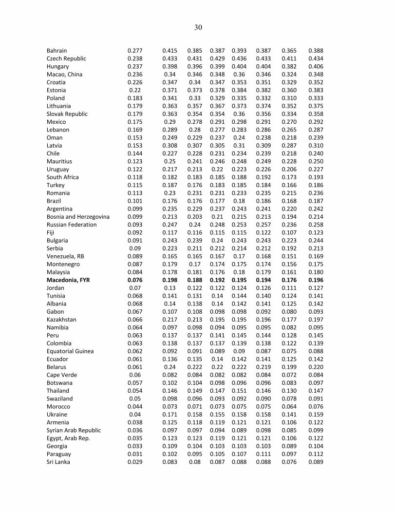
In Table A1 we report the calculations of real consumption for all 124 countries. In Table

A2 we report the estimates of the AIDS expenditure function, listing first the R2 values for the

share equations for each product and then the parameters α, β and Γ.24

Table A1: Comparisons of Real Consumption and real GDP, 2005

(USA = 1)

Country Nominal 

Consumption Per Capita 

Consumption indexes 

Using AIDS expenditure function and reference 

prices from:  GearyKhamis 

Fisher  GEKS  CCD Geary‐Khamis 

Neary, GAIA 

Diewert 

  (1)  (2) (3) (4) (5) (6) (7)  (8)

Iceland  1.248  0.771 0.786 0.794 0.795 0.790 0.779  0.791Norway  1.099  0.747 0.75 0.758 0.768 0.756 0.743  0.757Luxembourg  1.071  0.925 0.912 0.919 0.924 0.912 0.907  0.913Switzerland  1.043  0.733 0.743 0.739 0.749 0.750 0.737  0.751United States  1.000  1.000 1.000 1.000 1.000 1.000 1.000  1.000Denmark  0.982  0.673 0.678 0.685 0.69 0.687 0.671  0.688United Kingdom  0.895  0.775 0.766 0.793 0.807 0.779 0.767  0.779Ireland  0.843  0.64 0.654 0.662 0.648 0.664 0.648  0.665Sweden  0.838  0.681 0.695 0.693 0.696 0.694 0.679  0.695Austria  0.814  0.761 0.753 0.779 0.791 0.768 0.756  0.769France  0.775  0.699 0.702 0.716 0.726 0.705 0.690  0.706Finland  0.773  0.608 0.613 0.623 0.63 0.621 0.603  0.623Netherlands  0.756  0.706 0.702 0.72 0.736 0.698 0.682  0.699Japan  0.743  0.633 0.646 0.618 0.625 0.659 0.642  0.660Belgium  0.735  0.66 0.67 0.671 0.679 0.672 0.655  0.673Canada  0.731  0.729 0.731 0.735 0.733 0.740 0.727  0.741Germany  0.727  0.668 0.665 0.67 0.683 0.670 0.653  0.671Australia  0.722  0.683 0.699 0.701 0.702 0.704 0.688  0.704Italy  0.679  0.625 0.613 0.636 0.648 0.633 0.615  0.634New Zealand  0.606  0.575 0.578 0.59 0.599 0.596 0.577  0.597Cyprus  0.597  0.649 0.628 0.67 0.691 0.668 0.652  0.669Spain  0.582  0.623 0.614 0.648 0.677 0.633 0.616  0.634Greece  0.541  0.609 0.6 0.637 0.667 0.630 0.613  0.631Hong Kong, China  0.504  0.645 0.634 0.634 0.634 0.635 0.618  0.636Portugal  0.441  0.491 0.483 0.5 0.515 0.502 0.482  0.504Israel  0.422  0.511 0.516 0.516 0.52 0.517 0.497  0.519Malta  0.397  0.55 0.541 0.573 0.593 0.576 0.557  0.577Slovenia  0.378  0.488 0.489 0.499 0.505 0.505 0.484  0.506Singapore  0.377  0.505 0.501 0.498 0.503 0.507 0.486  0.508Taiwan, China  0.324  0.572 0.588 0.549 0.553 0.574 0.554  0.575Korea, Rep.  0.297  0.38 0.389 0.375 0.378 0.382 0.360  0.383

24 These estimates are taken from Feenstra, Ma and Prasada Rao (2009).

30

Bahrain  0.277  0.415 0.385 0.387 0.393 0.387 0.365  0.388Czech Republic  0.238  0.433 0.431 0.429 0.436 0.433 0.411  0.434Hungary  0.237  0.398 0.396 0.399 0.404 0.404 0.382  0.406Macao, China  0.236  0.34 0.346 0.348 0.36 0.346 0.324  0.348Croatia  0.226  0.347 0.34 0.347 0.353 0.351 0.329  0.352Estonia  0.22  0.371 0.373 0.378 0.384 0.382 0.360  0.383Poland  0.183  0.341 0.33 0.329 0.335 0.332 0.310  0.333Lithuania  0.179  0.363 0.357 0.367 0.373 0.374 0.352  0.375Slovak Republic  0.179  0.363 0.354 0.354 0.36 0.356 0.334  0.358Mexico  0.175  0.29 0.278 0.291 0.298 0.291 0.270  0.292Lebanon  0.169  0.289 0.28 0.277 0.283 0.286 0.265  0.287Oman  0.153  0.249 0.229 0.237 0.24 0.238 0.218  0.239Latvia  0.153  0.308 0.307 0.305 0.31 0.309 0.287  0.310Chile  0.144  0.227 0.228 0.231 0.234 0.239 0.218  0.240Mauritius  0.123  0.25 0.241 0.246 0.248 0.249 0.228  0.250Uruguay  0.122  0.217 0.213 0.22 0.223 0.226 0.206  0.227South Africa  0.118  0.182 0.183 0.185 0.188 0.192 0.173  0.193Turkey  0.115  0.187 0.176 0.183 0.185 0.184 0.166  0.186Romania  0.113  0.23 0.231 0.231 0.233 0.235 0.215  0.236Brazil  0.101  0.176 0.176 0.177 0.18 0.186 0.168  0.187Argentina  0.099  0.235 0.229 0.237 0.243 0.241 0.220  0.242Bosnia and Herzegovina  0.099  0.213 0.203 0.21 0.215 0.213 0.194  0.214Russian Federation  0.093  0.247 0.24 0.248 0.253 0.257 0.236  0.258Fiji  0.092  0.117 0.116 0.115 0.115 0.122 0.107  0.123Bulgaria  0.091  0.243 0.239 0.24 0.243 0.243 0.223  0.244Serbia  0.09  0.223 0.211 0.212 0.214 0.212 0.192  0.213Venezuela, RB  0.089  0.165 0.165 0.167 0.17 0.168 0.151  0.169Montenegro  0.087  0.179 0.17 0.174 0.175 0.174 0.156  0.175Malaysia  0.084  0.178 0.181 0.176 0.18 0.179 0.161  0.180Macedonia, FYR  0.076  0.198 0.188 0.192 0.195 0.194 0.176  0.196Jordan  0.07  0.13 0.122 0.122 0.124 0.126 0.111  0.127Tunisia  0.068  0.141 0.131 0.14 0.144 0.140 0.124  0.141Albania  0.068  0.14 0.138 0.14 0.142 0.141 0.125  0.142Gabon  0.067  0.107 0.108 0.098 0.098 0.092 0.080  0.093Kazakhstan  0.066  0.217 0.213 0.195 0.195 0.196 0.177  0.197Namibia  0.064  0.097 0.098 0.094 0.095 0.095 0.082  0.095Peru  0.063  0.137 0.137 0.141 0.145 0.144 0.128  0.145Colombia  0.063  0.138 0.137 0.137 0.139 0.138 0.122  0.139Equatorial Guinea  0.062  0.092 0.091 0.089 0.09 0.087 0.075  0.088Ecuador  0.061  0.136 0.135 0.14 0.142 0.141 0.125  0.142Belarus  0.061  0.24 0.222 0.22 0.222 0.219 0.199  0.220Cape Verde  0.06  0.082 0.084 0.082 0.082 0.084 0.072  0.084Botswana  0.057  0.102 0.104 0.098 0.096 0.096 0.083  0.097Thailand  0.054  0.146 0.149 0.147 0.151 0.146 0.130  0.147Swaziland  0.05  0.098 0.096 0.093 0.092 0.090 0.078  0.091Morocco  0.044  0.073 0.071 0.073 0.075 0.075 0.064  0.076Ukraine  0.04  0.171 0.158 0.155 0.158 0.158 0.141  0.159Armenia  0.038  0.125 0.118 0.119 0.121 0.121 0.106  0.122Syrian Arab Republic  0.036  0.097 0.097 0.094 0.089 0.098 0.085  0.099Egypt, Arab Rep.  0.035  0.123 0.123 0.119 0.121 0.121 0.106  0.122Georgia  0.033  0.109 0.104 0.103 0.103 0.103 0.089  0.104Paraguay  0.031  0.102 0.095 0.105 0.107 0.111 0.097  0.112Sri Lanka  0.029  0.083 0.08 0.087 0.088 0.088 0.076  0.089

31

Indonesia  0.028  0.073 0.072 0.073 0.074 0.075 0.064  0.076Philippines  0.026  0.071 0.071 0.07 0.071 0.070 0.060  0.071Moldova  0.026  0.111 0.101 0.097 0.097 0.094 0.081  0.095Lesotho  0.026  0.06 0.058 0.055 0.054 0.053 0.045  0.054Azerbaijan  0.025  0.097 0.094 0.094 0.095 0.095 0.082  0.096Sudan  0.025  0.051 0.05 0.054 0.051 0.052 0.044  0.053Bolivia  0.024  0.091 0.09 0.089 0.089 0.088 0.076  0.089China  0.023  0.06 0.06 0.056 0.057 0.054 0.045  0.054São Tomé and Principe  0.023  0.043 0.042 0.044 0.044 0.043 0.035  0.043Cameroon  0.022  0.043 0.041 0.045 0.045 0.044 0.037  0.045Iraq  0.021  0.068 0.064 0.06 0.059 0.059 0.050  0.060Senegal  0.021  0.04 0.04 0.041 0.042 0.039 0.032  0.039Nigeria  0.019  0.039 0.041 0.04 0.039 0.034 0.028  0.034Côte d'Ivoire  0.019  0.033 0.032 0.034 0.035 0.034 0.027  0.034Congo, Rep.  0.018  0.035 0.035 0.032 0.032 0.028 0.023  0.029Mongolia  0.018  0.061 0.058 0.052 0.051 0.050 0.042  0.051Angola  0.016  0.022 0.022 0.022 0.022 0.019 0.015  0.020Kenya  0.015  0.039 0.04 0.038 0.039 0.038 0.031  0.038Benin  0.015  0.033 0.032 0.033 0.034 0.030 0.025  0.031Kyrgyz Republic  0.014  0.07 0.065 0.063 0.063 0.060 0.051  0.061India  0.014  0.049 0.047 0.046 0.047 0.047 0.039  0.047Chad  0.013  0.03 0.03 0.029 0.027 0.027 0.021  0.027Togo  0.013  0.027 0.026 0.027 0.028 0.026 0.021  0.027Vietnam  0.012  0.052 0.048 0.043 0.042 0.040 0.032  0.040Cambodia  0.012  0.044 0.042 0.039 0.039 0.037 0.030  0.037Mali  0.011  0.023 0.023 0.023 0.023 0.022 0.017  0.022Central African Republic  0.01  0.02 0.019 0.02 0.021 0.019 0.015  0.019Burkina Faso  0.01  0.025 0.023 0.025 0.026 0.025 0.020  0.026Lao PDR  0.01  0.038 0.037 0.035 0.035 0.033 0.026  0.033Nepal  0.009  0.031 0.028 0.029 0.029 0.029 0.024  0.030Sierra Leone  0.009  0.026 0.025 0.023 0.022 0.019 0.015  0.019Tajikistan  0.009  0.062 0.053 0.047 0.045 0.040 0.033  0.040Madagascar  0.008  0.026 0.025 0.024 0.023 0.022 0.017  0.022Rwanda  0.007  0.019 0.018 0.018 0.019 0.019 0.015  0.019Guinea  0.007  0.021 0.022 0.02 0.02 0.017 0.013  0.017Malawi  0.006  0.018 0.017 0.016 0.016 0.014 0.011  0.014Niger  0.006  0.014 0.013 0.014 0.014 0.013 0.010  0.013Guinea‐Bissau  0.006  0.013 0.012 0.013 0.012 0.012 0.010  0.013Liberia  0.004  0.01 0.01 0.008 0.008 0.007 0.005  0.007Congo, Dem. Rep.  0.003  0.004 0.004 0.004 0.004 0.004 0.003  0.004

mean  0.227  0.265 0.263 0.265 0.269 0.266 0.252  0.267variance  0.096  0.064 0.064 0.066 0.068 0.067 0.065  0.067std. error of mean  0.028  0.023 0.023 0.023 0.024 0.023 0.023  0.023

Source: Authors’ calculations as explained in the text.

Notes: Table 1 reports results for selected countries, shown here in bold.

n.a. not available due to missing data

32

Table A2: Parameter Estimates for AIDS

Category R2

Food and non-alcoholic beverages 0.736 0.183 -0.193 0.050 -0.035 -0.012 -0.047 0.001 -0.021 -0.023 0.013 0.034 -0.062 0.079 0.024

Alcoholic beverages and tobacco 0.172 0.033 0.004 -0.035 -0.017 0.011 -0.030 0.003 -0.016 0.037 -0.008 0.025 0.009 0.012 0.010

Clothing and footwear 0.075 0.050 -0.005 -0.012 0.011 0.009 -0.007 -0.010 -0.011 0.011 0.025 -0.029 0.016 0.020 -0.022

Gross Rent, water, fuel and power 0.407 0.158 0.017 -0.047 -0.030 -0.007 0.108 0.005 -0.002 0.011 -0.003 -0.016 -0.005 0.004 -0.017

Household furnishings 0.123 0.053 0.007 0.001 0.003 -0.010 0.005 -0.027 -0.008 -0.003 0.004 0.043 0.009 0.017 -0.033

Medical and health services 0.407 0.093 0.029 -0.021 -0.016 -0.011 -0.002 -0.008 0.021 0.029 0.001 -0.007 0.008 -0.002 0.010

Transport 0.218 0.104 0.035 -0.023 0.037 0.011 0.011 -0.003 0.029 -0.041 0.001 0.051 -0.066 -0.047 0.041

Communication 0.167 0.027 0.008 0.013 -0.008 0.025 -0.003 0.004 0.001 0.001 -0.009 0.006 -0.001 -0.006 -0.023

Recreation 0.641 0.070 0.044 0.034 0.025 -0.029 -0.016 0.043 -0.007 0.051 0.006 -0.061 0.027 -0.025 -0.046

Education 0.136 0.078 -0.001 -0.062 0.009 0.016 -0.005 0.009 0.008 -0.066 -0.001 0.027 0.005 0.025 0.035

Restaurants 0.325 0.057 0.017 0.079 0.012 0.020 0.004 0.017 -0.002 -0.047 -0.006 -0.025 0.025 -0.111 0.035

Other goods and services 0.507 0.093 0.038 0.024 0.010 -0.022 -0.017 -0.033 0.010 0.041 -0.023 -0.046 0.035 0.035 -0.014

Note： This table presents the AIDS estimation results for parameters , , and in equation (7). R2 gives the goodness of fit for the

estimated virtual budget share of each commodity across all countries.

33

Appendix B: Regression Methodology for Chinese Price Adjustments

We estimate separate regressions for the following nine commodity groups within

consumption: food and non-alcoholic beverages; clothing and footwear; gross rent, water, fuel

and power; medical and health services; transport; recreation; education; restaurants; other goods

and services. Three other commodity groups had incomplete data and so no adjustment was

made for: alcoholic beverages and tobacco; household furnishings; and communication. The

sample consisted of 22 developing countries in the Asia-Pacific region. Country coverage and

the procedures adopted by the Asian Development Bank are detailed in their final report (ADB,

2007). China is not included in any of the regressions since its inclusion may result in biased

regression coefficients if the Chinese prices are understated in the first place.

Two regression specifications were used: linear and log-linear models:

Linear: ij ij ijY X u , and Log-linear: ln lni i iY X u

where iY is the price level of the i-th commodity group in country j, defined as the ratio of the

PPP for the i-th commodity group in country j to the market exchange rate for the currency of

that country. Separate regressions were run for each commodity group i. We consider four

alternative regressor variables leading to four different model specifications, as described in the

text. In addition, we estimate two sets of models, one including Fiji and another without Fiji. As

Fiji is an island country where most consumption items are imported, the price level in Fiji is

considerably higher than we would expect from countries at a similar level of development.

Further, Fiji price data suffered from a strong urban bias in the collection of ICP prices.

Taking account of all the combinations of alternative X variables, linear versus log-linear

models, and inclusion/exclusion of Fiji, we estimate a total of 16 alternative specifications.25 In

25 Detailed results for all sixteen models are available from the authors.

34

order to be able to compare the performance of linear models against log-linear models, we do

not use the conventional correlation coefficient but rather an alternative R2 measure, defined as

the squared correlation between observed and predicted Y values. Based on R2 , the log-linear

specification with a dummy variable for Fiji dominates the linear specification in all cases, so we

only report results for the former. Estimated coefficients and the R2 values for Models 1 to 4

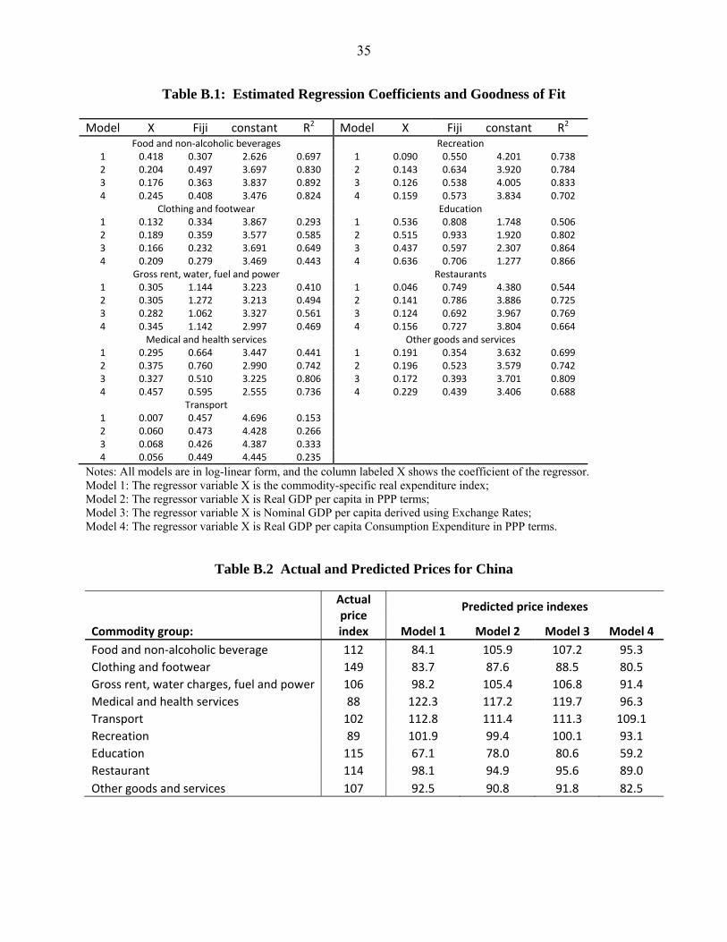
estimated for the nine commodity groups are presented for the log-linear model in Table B.1.

Our preferred models conceptually are Models 1 and 4 followed by Models 2 and 3. The models

offer satisfactory fits for most of the commodity groups except for transport. Table B.2 shows

the actual and estimated price indexes for different commodity groups derived using models 1 to

4.

35

Table B.1: Estimated Regression Coefficients and Goodness of Fit Model  X  Fiji  constant  R2 Model  X  Fiji  constant  R2 

Food and non‐alcoholic beverages  Recreation 1  0.418  0.307  2.626  0.697  1  0.090  0.550  4.201  0.738 2  0.204  0.497  3.697  0.830  2  0.143  0.634  3.920  0.784 3  0.176  0.363  3.837  0.892  3  0.126  0.538  4.005  0.833 4  0.245  0.408  3.476  0.824  4  0.159  0.573  3.834  0.702 

Clothing and footwear  Education 1  0.132  0.334  3.867  0.293  1  0.536  0.808  1.748  0.506 2  0.189  0.359  3.577  0.585  2  0.515  0.933  1.920  0.802 3  0.166  0.232  3.691  0.649  3  0.437  0.597  2.307  0.864 4  0.209  0.279  3.469  0.443  4  0.636  0.706  1.277  0.866 

Gross rent, water, fuel and power  Restaurants 1  0.305  1.144  3.223  0.410  1  0.046  0.749  4.380  0.544 2  0.305  1.272  3.213  0.494  2  0.141  0.786  3.886  0.725 3  0.282  1.062  3.327  0.561  3  0.124  0.692  3.967  0.769 4  0.345  1.142  2.997  0.469  4  0.156  0.727  3.804  0.664 

Medical and health services  Other goods and services 1  0.295  0.664  3.447  0.441  1  0.191  0.354  3.632  0.699 2  0.375  0.760  2.990  0.742  2  0.196  0.523  3.579  0.742 3  0.327  0.510  3.225  0.806  3  0.172  0.393  3.701  0.809 4  0.457  0.595  2.555  0.736  4  0.229  0.439  3.406  0.688 

Transport           1  0.007  0.457  4.696  0.153           2  0.060  0.473  4.428  0.266           3  0.068  0.426  4.387  0.333           4  0.056  0.449  4.445  0.235           

Notes: All models are in log-linear form, and the column labeled X shows the coefficient of the regressor. Model 1: The regressor variable X is the commodity-specific real expenditure index; Model 2: The regressor variable X is Real GDP per capita in PPP terms; Model 3: The regressor variable X is Nominal GDP per capita derived using Exchange Rates; Model 4: The regressor variable X is Real GDP per capita Consumption Expenditure in PPP terms.

Table B.2 Actual and Predicted Prices for China

 Actual price index 

Predicted price indexes 

Commodity group:  Model 1   Model 2  Model 3   Model 4  

Food and non‐alcoholic beverage  112  84.1  105.9  107.2  95.3 

Clothing and footwear  149  83.7  87.6  88.5  80.5 

Gross rent, water charges, fuel and power 106  98.2  105.4  106.8  91.4 

Medical and health services  88  122.3  117.2  119.7  96.3 

Transport   102  112.8  111.4  111.3  109.1 

Recreation   89  101.9  99.4  100.1  93.1 

Education  115  67.1  78.0  80.6  59.2 

Restaurant   114  98.1  94.9  95.6  89.0 

Other goods and services  107  92.5  90.8  91.8  82.5 

36

Appendix C: Proof of Proposition 1

We first derive a reduced system either in the international prices vector, Π, or in the

output-based real exchange rates, RO. Following Neary (2004), we start with an international

price vector Π0 which is positive. Then using Π0 in (19), we get a value for ROj for j=1,2,…,C.

Substituting these ROj’s into (16), (17) and (18) yields a new price vector Π1. Thus we have a

function that maps Π0 to Π1. We represent this relationship by:

1 1( ) or in general, ( )o t tH H (C1)

Equation (C1) represents a system of non-linear simultaneous equations. We can state the

following general properties of H: (i) H is positive for all Π0 >0 ; (ii) H is linearly homogeneous;

and (iii) H is a continuous function. These properties follow from the structure of the equations

(16) to (19) and the assumed properties of the revenue function.

Further we observe that if Π is a solution to equations (16) to (19), then kΠ is also a

solution for any k>0. Thus any solution is unique up to a factor of proportionality. Thus we can

restrict ourselves to solutions of (C1) up to a linear restriction 2

11

M N

ii

with πi > 0. This

basically means the mapping H in (C1) is a mapping from the unit simplex into itself. Further H

is continuous. From Brouwer’s fixed point theorem it follows that there exists a fixed point Π*

such that Π*=H (Π*). We note here that uniqueness of the fixed point is not guaranteed by this

theorem.26

UC Davis and NBER Tsinghua University Oxford University and CEPR University of Queensland First submitted: 20 September 2011 Accepted: 25 September 2012

26 Likewise, Neary (2004) proves the existence of a unique positive solution to the Geary system but only shows the existence of a positive solution to the GAIA system.

37

References

Afriat, S. (1967). 'The construction of utility functions from expenditure data,' International Economic Review, vol. 8(1), pp. 67–77.

Allen, R. G. D. (1949),’The economic theory of index numbers,’Economica,16, pp. 197–203.

Asian Development Bank (2007), Purchasing Power Parities and Real Expenditures, Manila, Philippines.

Balk, B. M. (2008), Price and Quantity Index Numbers: Models for Measuring Aggregate Change and Difference, New York: Cambridge University Press,

Balk, B. M., (2009), ‘Aggregation methods in international comparisons: An evaluation’, in Purchasing Power Parities of Currencies; Recent Advances in Methods and Applications, edited by D. S. Prasada Rao, Edward Elgar: Cheltenham, UK.

Banks, J., Blundell, R. and Lewbel, A. (1997), ‘Quadratic Engel curves and consumer demand,’Review of Economics and Statistics, 79(4), pp. 527–39.

Barnett, W. A., Diewert, W. E. and Zellner, A. (2009), ‘Introduction to measurement with theory,’ Macroeconomic Dynamics, 13(S2), pp. 151-68.

Caves, D. W., Christensen, L. R. and Diewert, W. E. (1982a), ‘The economic theory of index numbers and the measurement of input, output, and productivity,’ Econometrica, 50(6), pp. 1393-414.

Caves, D. W., Christensen, L. R. and Diewert, W. E., (1982b), ‘Multilateral comparisons of output, input, and productivity using superlative index numbers,’ Economic Journal, 92, March, pp. 73-86.

Crawford, I. and Neary, J.P. (2008). ‘Testing for a reference consumer in international

comparisons of living standards’, American Economic Review, vol. 98(4), pp. 1731–2.

Deaton, A. and Heston, A. (2010), ‘Understanding PPPs and PPP-based national accounts,’ American Economic Journal: Macroeconomics, 2(4), pp. 1-35.

Deaton, A and Muellbauer, J. (1980), ‘An almost ideal demand system,’American Economic Review, 70(3), pp. 312-26.

Diewert, W. E (1976), ‘Exact and superlative index numbers,’Journal of Econometrics, 4(2), pp. 115-45.

Diewert, W. E. (1999), ‘Axiomatic and economic approaches to international comparisons,’ in (A. Heston and R.E. Lipsey eds.), International and Interarea Comparisons of Income, Output and Prices, Studies in Income and Wealth, Volume 61, pp. 13-87, Chicago: The University of Chicago Press.

38

Diewert, W. E. (2010a), ‘Understanding PPPs and PPP-based national accounts: Comment,’ American Economic Journal: Macroeconomics, 2(4), pp. 36-45.

Diewert, W. E. (2010b), ‘New methodological developments for the International Comparison Program’, Review of Income and Wealth, Series56, Special Issue 1, S11-31.

Diewert, W. E. and Morrison, C. J. (1986), ‘Adjusting outputs and productivity indexes for changes in the terms of trade,’ ECONOMIC JOURNAL, 96, pp. 659-79.

Diewert, W. E. and Wales, T. C. (1988), ‘A normalized quadratic semiflexible functional form’, Journal of Econometrics 37, pp. 327-42.

Feenstra, R. C., Heston, A., Timmer, M. P. and Deng, H. (2009), ‘Estimating real production and expenditures across countries: a proposal for improving the Penn World Tables,’ Review of Economics and Statistics, 91(1), pp. 201-12.

Feenstra, R. C., Inklaar, R.and Timmer, M. P. (2012), ‘The next generation of the Penn World Table,’ University of California, Davis and University of Groningen.

Feenstra, R. C., Ma, H.and Rao , D.S. P. (2009), ‘Consistent comparisons of real income across countries and over time,’ Macroeconomic Dynamics, 13(S2), pp. 169-93.

Feenstra, R. C. and Romalis, J. (2012). ‘International prices and endogenous quality,’ University of California, Davis and Australian National University.

Feenstra, R. C., Ma, H., Neary, J. P. and Rao, D.S. P., (2012), ‘Who shrunk China? Puzzles in the measurement of real GDP,’ Working Paper No. 17729, NBER.

Geary, R.C. (1958), ‘A note on the comparison of exchange rates and purchasing power between countries’, Journal of the Royal Statistical Society, Series A, 121(1), pp. 97-9.

Gerschenkron, A. (1951), A Dollar Index of Soviet Machinery Output, 192728 to 1937, Report R-197, Santa Monica: Rand Corporation.

Heston, A. (2007), ‘What can be learned about the economics of China and India from the results of purchasing power comparisons?’ Paper delivered to the Conference on India and China’s Role in International Trade and Finance and Global Economic governance, ICRIER, New Delhi, December 6-7, 2007.

Honohan, P. (2001), ‘Does PPP-adjusted data exaggerate the relative size of poor economies?’ Applied Economics Letters, 8(12), pp. 799-802.

Khamis, S. H. (1970), ‘Properties and conditions for the existence of a new type of index numbers’, Sankhya, Series B, 32, pp. 81-98.

Khamis, S. H. (1972), ‘A new system of index numbers for national and international purposes’, Journal of the Royal Statistical Society, Series A, 135(1), pp. 96–121.

39

Kohli, R. (2004), ‘Real GDP, real domestic income, and terms-of-trade changes,’ Journal of International Economics, 62(1), pp. 83-106.

Maddison, A. (2007), ‘Measuring the Performance of Transition Economics: Some Lessons from Chinese Experience,’ keynote address to the Beijing Conference of IARIW and NBS, September 19.

Neary, J. P. (2004), ‘Rationalizing the Penn World Table: true multilateral indexes for international comparisons of real income,’ American Economic Review, 94(5), pp. 1411-28.

Samuelson, P. A. (1974), ‘Analytical notes on international real-income measures,’ ECONOMIC JOURNAL, 84:335, pp. 595-608.

Sanyal, K. K. and R. W. Jones (1982), ‘The theory of trade in middle products,’American Economic Review, 72(1), pp. 16-31.

Varian, H.R. (1990). 'Goodness-of-fit in optimizing models,' Journal of Econometrics, vol. 46(1–2), pp. 125–40.

World Bank, 2007, World Development Indicators, Washington, DC. (CD)

World Bank, 2008a, World Development Indicators, Washington, DC. (CD and online)

World Bank, 2008b, Global Purchasing Power Parities and Real Expenditures – 2005 International Comparison Program, World Bank, Washington DC. URL: http://siteresources.worldbank.org/ICPINT/Resources/icp-final.pdf; accessed 18 March, 2010.

40

Table 1: Real Consumption for Selected Countries, 2005 (USA = 100)

Nominal consump. per capita

Consumption Indexes Using AIDS expenditure

function and reference prices from:

Countries Geary-Khamis

Fisher GEKS CCD Geary-Khamis

Neary, GAIA

Diewert

(1) (2) (3) (4) (5) (6) (7) (8)

United States 100 100 100 100 100 100 100 100

%diff from GEKS 0.00 0.00 0.00 0.00 0.00 0.00 0.00

United Kingdom 89.5 77.5 76.6 79.3 80.7 77.9 76.7 77.9

%diff from GEKS -2.27 -3.40 0.00 1.77 -1.77 -3.28 -1.77 Ireland 84.3 64.0 65.4 66.2 64.8 66.4 64.8 66.5

%diff from GEKS -3.32 -1.21 0.00 -2.11 0.30 -2.11 0.45 Netherlands 75.6 70.6 70.2 72 73.6 69.8 68.2 69.9

%diff from GEKS -1.94 -2.50 0.00 2.22 -3.06 -5.28 -2.92 Canada 73.1 72.9 73.1 73.5 73.3 74 72.7 74.1

%diff from GEKS -0.82 -0.54 0.00 -0.27 0.68 -1.09 0.82 Korea, Rep. 29.7 38.0 38.9 37.5 37.8 38.2 36 38.3

%diff from GEKS 1.33 3.73 0.00 0.80 1.87 -4.00 2.13 Macedonia 7.6 19.8 18.8 19.2 19.5 19.4 17.6 19.6

%diff from GEKS 3.13 -2.08 0.00 1.56 1.04 -8.33 2.08 China 2.3 6.0 6.0 5.6 5.7 5.4 4.5 5.4

%diff from GEKS 7.14 7.14 0.00 1.79 -3.57 -19.64 -3.57 India 1.4 4.9 4.7 4.6 4.7 4.7 3.9 4.7

%diff from GEKS 6.52 2.17 0.00 2.17 2.17 -15.22 2.17

mean of %diff from GEKS 2.330 0.211 0.000 0.833 -1.085 -11.727 -0.405

s.e. of the mean difference (0.54) (0.449) (0.00) (0.191) (0.409) (0.830) (0.402)

Regression of index on GEKS 0.981 0.990 1.000 1.005 1.021 1.081 1.017

s.e. of slope coefficient (0.004) (0.005) `(0.000) (0.002) (0.004) (0.005) (0.004) Source: Authors’ calculations using 2005 ICP benchmark program data. Notes: Each row reports indexes for real consumption expenditure for selected countries relative to the U.S., followed by a row showing the percentage difference of each index relative to the GEKS for the same country. Column (1) gives the nominal consumption expenditure (obtained using exchange rates for converting national currency data into U.S. dollars) per capita in 2005, relative to the U.S. Column (2) gives the Geary-Khamis calculation of real consumption, while column (3) gives the bilateral Fisher index relative to the United States. Columns (4)-(5) present flexible weight measures of real consumption expenditure per capita, using respectively the GEKS, and CCD methods, as defined in the text in equations (4)-(5). Columns (6) to (8) show measures of real consumption based on the estimated AIDS expenditure function, using different reference prices: column (6) uses the Geary-Khamis reference prices; column (7) uses the GAIA reference prices; and column (8) uses every country’s prices as

41

reference and then takes the geometric mean of the results, as in Barnett, Diewert and Zellner (2009). The last four rows are for the sample of 124 countries, where the last two rows report the slope coefficient (and standard error) from a regression of the natural log of each index on the log of the GEKS index.

42

Table 2: Real Consumption for China with Adjusted Prices, 2005 (USA = 100)

Method of adjusting Chinese prices

Consumption Indexes

Using AIDS expenditure function and reference prices

from: Geary-Khamis

Fisher GEKS CCD Geary-Khamis

Neary, GAIA

Diewert

(2) (3) (4) (5) (6) (7) (8)

20% reduction in prices 7.5 7.5 7.1 7.1 6.8 5.8 6.8

%diff from China in Table 1 25.0 25.0 26.8 24.6 25.9 28.9 25.9 Regression model 1 7.0 6.8 6.6 6.6 6.7 5.6 6.9

%diff from China in Table 1 16.7 13.3 17.9 15.8 24.1 24.4 27.8 Regression model 2 6.5 6.5 6.1 6.2 5.9 4.9 5.9

%diff from China in Table 1 8.3 8.3 8.9 8.8 9.3 8.9 9.3 Regression model 3 6.4 6.4 6.0 6.1 5.8 4.8 5.9

%diff from China in Table 1 6.7 6.7 7.1 7.0 7.4 6.7 9.3 Regression model 4 7.4 7.3 6.8 6.9 6.6 5.5 6.6

%diff from China in Table 1 23.3 21.7 21.4 21.1 22.2 22.2 22.2 Source: Authors’ calculations using 2005 ICP benchmark program data and ADB (2007).

Notes: See notes to Table 1. Each row here gives the results from used adjusted consumption prices for

China, and the corresponding percentage difference relative to the China estimate in Table 1. Besides

adjusting all Chinese prices downward by 20%, we take four log-linear regression models to adjust

Chinese prices, as described in Appendix B. Model 1 uses real per capita expenditure index specific to the

commodity group as the regressor variable. Model 2 uses real GDP per capita index in PPP terms. Model

3 uses nominal GDP per capita index in a common currency. Model 4 uses real per capita index for

private consumption in PPP terms instead of the index for the whole of GDP.

43

Table 3: Actual and Reference Prices

Category Sample MeanUnited States Geary-Khamis

Neary, GAIA

South Korea

Food and non-alcoholic beverages 1 1.100 0.922 0.800 1.627

Alcoholic beverages and tobacco 1 1.395 0.872 0.587 1.162 Clothing & footwear 1 1.136 0.852 0.670 1.257

Gross rent, water, fuel and power 1 1.889 1.034 0.820 1.446 Household furnishings 1 1.302 0.898 0.589 0.988

Medical and health services 1 2.995 1.082 4.023 1.047 Transport 1 0.950 0.772 0.953 1.023

Communication 1 1.128 0.722 0.816 0.641 Recreation 1 1.231 0.788 0.663 1.121

Education 1 3.412 1.023 1.298 1.602 Restaurants 1 1.025 0.797 0.802 1.310

Other goods and services 1 1.632 1.000 1.000 1.215 b(p) 1 1.054 0.992 1.053 0.930

Source: Authors’ calculations using 2005 ICP benchmark program data.

Notes. Listed are the reference prices used in the calculations for Table 1 and Appendix Table

A1. Since all prices have been normalized by the sample mean (over 124 countries), the prices p

= 1 represent the sample mean. The second set of prices are for the U.S. The third set of

reference prices are the GK prices computed as in equations (1)-(2), the fourth set are the GAIA

reference prices computed as in (9)-(10), and the final set of prices are for South Korea. The final

row is computed as ( ) iii

b p p using the estimates from Appendix Table A2.