WHITE PAPER

Fracture Conductivity and Cleanup in GOHFER® Software

Fracture Conductivity and Cleanup in GOHFER® SoftwareAuthorR. D. Barree

INTRODUCTION

There has been considerable interest in, as well as requests for additional information and clarification on, the representation of fracture conductivity and cleanup within GOHFER® software. The following discussion outlines the current process of generating useful fracture conductivity and effective length, developed from work conducted over the past 30 years by the Stim-Lab consortium, along with extensive laboratory and field work.

Fracture conductivity and cleanup are complex issues that relate to many aspects of the hydraulic fracturing process. In fact, the useful conductivity generated, and possibly the total exposed reservoir surface area, are the only net results that persist after the job is complete. To describe the development of conductivity, the following aspects of the process must be considered: fracture geometry, proppant transport and placement, leakoff and closure mechanisms, gel concentration and damage, stress on the proppant pack, interactions between the pack and the reservoir rock at the fracture walls, applied potential gradients during flowback and production, gravity and capillary effects (in the pack and at the fracture face), permeability as a function of velocity and saturation in the pack and surrounding reservoir, and the overall evolution of conductivity as related to the cleanup process.

WHITE PAPER

2

TABLE OF CONTENTS

Fracture Geometry and Proppant Placement . . . . . . . . . . . . . . . . . . . . . . . . . . . . . . . . . . . . . 4

Gel Damage Effects . . . . . . . . . . . . . . . . . . . . . . . . . . . . . . . . . . . . . . . . . . . . . . . . . . . . . . . . 4

Closure Stress on Proppant . . . . . . . . . . . . . . . . . . . . . . . . . . . . . . . . . . . . . . . . . . . . . . . . . . 6

Low Proppant Concentration and Wall Effects . . . . . . . . . . . . . . . . . . . . . . . . . . . . . . . . . . . . 6

Change in Closure Stress with Production . . . . . . . . . . . . . . . . . . . . . . . . . . . . . . . . . . . . . . . 7

Multi-Phase and Non-Darcy Effects on Conductivity . . . . . . . . . . . . . . . . . . . . . . . . . . . . . . . 8

Two-Phase Relative Permeability in Proppant Packs. . . . . . . . . . . . . . . . . . . . . . . . . . . . . . . . 8

Non-Darcy or Inertial Effects on Conductivity. . . . . . . . . . . . . . . . . . . . . . . . . . . . . . . . . . . . . 9

Gel Cleanup and Reservoir Energy . . . . . . . . . . . . . . . . . . . . . . . . . . . . . . . . . . . . . . . . . . . . 10

Filter-Cake Deposition and Erosion . . . . . . . . . . . . . . . . . . . . . . . . . . . . . . . . . . . . . . . . . . . . 10

Polymer Gel Residue and Damage . . . . . . . . . . . . . . . . . . . . . . . . . . . . . . . . . . . . . . . . . . . . 10

Velocity and Potential Gradients During Production and Cleanup. . . . . . . . . . . . . . . . . . . . . 11

Convergent Skin Effects for Horizontal Wells . . . . . . . . . . . . . . . . . . . . . . . . . . . . . . . . . . . . 11

Effective Conductivity in Oil Wells . . . . . . . . . . . . . . . . . . . . . . . . . . . . . . . . . . . . . . . . . . . . 12

Effective Conductivity in Gas Wells . . . . . . . . . . . . . . . . . . . . . . . . . . . . . . . . . . . . . . . . . . . 13

Degradation of Proppant Conductivity Over Time. . . . . . . . . . . . . . . . . . . . . . . . . . . . . . . . . 14

Capillary and Gravity Forces . . . . . . . . . . . . . . . . . . . . . . . . . . . . . . . . . . . . . . . . . . . . . . . . . 15

Derivation of Capillary Entry Pressure . . . . . . . . . . . . . . . . . . . . . . . . . . . . . . . . . . . . . . . . . 15

Capillary Entry Pressure for Shale and Tight-Sand Reservoirs . . . . . . . . . . . . . . . . . . . . . . . 15

Oil and Gas Migration Through the Proppant Pack . . . . . . . . . . . . . . . . . . . . . . . . . . . . . . . . 16

Capillary Entry Pressure of Proppant Packs for Various Sieves. . . . . . . . . . . . . . . . . . . . . . . 17

Flow Regimes in Vertical Transverse Fractures . . . . . . . . . . . . . . . . . . . . . . . . . . . . . . . . . . . 17

Effective Fracture Length and Dimensionless Conductivity . . . . . . . . . . . . . . . . . . . . . . . . . 18

Resaturation and Hysteresis Effects. . . . . . . . . . . . . . . . . . . . . . . . . . . . . . . . . . . . . . . . . . . 18

Dimensionless Fracture Conductivity . . . . . . . . . . . . . . . . . . . . . . . . . . . . . . . . . . . . . . . . . . 19

Problems with Dimensionless Conductivity and the McGuire-Sikora Curves . . . . . . . . . . . 20

Effective Flowing Length . . . . . . . . . . . . . . . . . . . . . . . . . . . . . . . . . . . . . . . . . . . . . . . . . . . 20

Proppant Cutoff Length, Flowing Length, and Effective Length in GOHFER Software . . . . .21

Multi-Cluster Stages in Horizontal Well Fracturing . . . . . . . . . . . . . . . . . . . . . . . . . . . . . . . . 22

Final Thoughts on Drainage Area and EUR . . . . . . . . . . . . . . . . . . . . . . . . . . . . . . . . . . . . . . 23

WHITE PAPER

3

FRACTURE GEOMETRY AND PROPPANT PLACEMENT

Proppant pack conductivity, kfwf, is primarily related to the thickness of the continuous proppant layer connected to the wellbore. This pack width is, therefore, fundamentally determined by the width of the fracture created rather than the injected slurry concentration. Pumping a high-concentration slurry does not result in a wider fracture. Fracture width is dependent on the fracture geometry (height, length, etc.), degree of anisotropy of the rock mass, stiffness of the system (fracture compliance), and net pressure during pumping. High mobility fluid systems such as slickwater tend to produce overall less net pressure, fracture height, and width, resulting in a lower maximum pack thickness. On the other hand, high-viscosity gelled fluid systems provide the opportunity to create more width, though they also carry the potential for more gel damage.

It is important to remember that, contrary to their representation in almost all fracture simulators, fracture walls are not smooth and regular. Rocks tend to break, or shear, along planes of weakness when subjected to imposed stress and strain. Shearing occurs along bedding planes, joints, natural fractures, inclusions, and wherever there are sudden changes in mechanical properties. During pumping, the fracture is more likely to resemble a series of fracture or joint segments with frequent offsets and possible pinch points, both in the lateral and vertical direction from the injection source. Due to settling and/or leakoff (and associated transverse particle migration), proppant tends to accumulate on ledges or at pinch points and leakoff sites, which, in turn, leads to rapid packing of the created fracture width at localized sites throughout the fracture. This mechanism has been demonstrated in hundreds of large-scale slot flow experiments conducted during the Stim-Lab fracturing fluid, rheology, and transport consortium. Some of these results have been published in SPE 67298.

Multiple processes cause holdup and proppant buildup during pumping by concentrating proppant near the injection point and reducing transport into the far field. The proppant pack, therefore, tends to accumulate until the created fracture width is filled, regardless of the input slurry concentration. Proppant holdup typically increases with low-viscosity fluids and in conditions of high secondary leakoff through existing “natural” or induced fractures and fissures in the primary hydraulic fracture walls. However, this does not necessarily mean that crosslinked fluids can be used to minimize holdup, as the fluid entering the fracture may not have the rheological properties expected or observed in surface tests.

Crosslinked fracturing fluids are shear thinning, and may require specific temperature and shear conditions to form a stable viscosity. Fluid entering the fracture is subjected to generally three to five minutes of high-shear flow in the pipe followed by a brief trip through the perforations and near-wellbore fracture. This fluid

is sheared so that a stable crosslink is highly unlikely. A crosslinked gel subjected to shear rates equivalent to thousands of reciprocal seconds for several minutes will not immediately re-form a stable gel structure. A well-formulated system may develop most of its structure (80% to 90% of peak viscosity) after a minute or so of stable low shear in the fracture. At typical fracture treatment velocity (1 fps to 2 fps), the fluid may be 100 ft from the injection site before it develops stable gel properties. In the near-wellbore area, the fluid more likely resembles a sheared linear gel.

Some fluid systems do not crosslink until a minimum target temperature is achieved. In the past, it was generally believed that static reservoir temperature is reached upon entry to the fracture. More recently, distributed temperature sensing (DTS) measurements via optical fibers have become more common, and the associated data show that temperature inside the wellbore cools well below the formation temperature with the first volume of fluid pumped. During high-rate injections, the well temperature can even approach surface temperature. The DTS data further show that fracture fluid temperature remains relatively cold for days, weeks, and sometimes months after the treatment is completed. If a crosslink system is designed to work at an elevated temperature, and the fluid never reaches that temperature, the entire job may be placed with the equivalent of a linear gel.

GEL DAMAGE EFFECTS

Proppant holdup is not inherently negative, though it must be accounted for in understanding treatment design and production response. When proppant settles and starts to accumulate, areas of the fracture near the injection point will become packed, from wall to wall of the fracture, with proppant. The first proppant injected may accumulate near the well, which is often apparent in the tracer log by the presence of the first injected radioactive tracer remaining within the radius of investigation (even at the end of the job). It may also be indicated by flowback, during cleanup or production, of the 100-mesh sand injected as “scour” at the start of the job.

Proppant holdup effectively concentrates proppant, filling the fracture to its maximum attainable concentration regardless of the injected slurry concentration. A second benefit is that fracturing fluid within the pore space of the accumulated proppant pack will have a gel concentration close to the injected polymer load. It is possible that some filter cake may be deposited during the pad stage and could affect ultimate conductivity, though the bulk of this fluid will be relatively unconcentrated. This is important because the polymers used in fracturing fluids cannot exit the fracture or enter the pore space of the reservoir. All polymer injected throughout the treatment, including all pad and sand-laden fluid, must remain in the created fracture volume. At closure, this suggests that the polymer will be concentrated in the remaining pore volume of the proppant pack.

WHITE PAPER

4

Figure 1 is a simple overall fracture material balance showing the concentration of polymer residue in the pack at closure. Open volume of unpropped fractures is not considered. The x-axis is the total pounds of proppant pumped during the job, divided by the total gallons of pad and sand-laden fluid. Assuming a sand-specific gravity for the proppant and average pack porosity (from Stim-Lab tests), the total pore volume of the proppant pack can be estimated. The pore volume, at closure, divided by the total fluid volume represents a concentration factor. All polymer dispersed in the injected fluid must end up residing in the remaining pack pore space. The y-axis shows the folds of increase in gel concentration resulting from different average proppant concentrations (APCs). For example, at APC=1 (100,000 lb of sand in 1,000,000 gal of fluid), the concentration factor is 38.2. Based on this, a 10-ppt linear gel would leave a residue of approximately 380 ppt in the proppant pack. Gel concentration near the well should be close to 1, not including filter cake, due to proppant settling and holdup. This suggests that, at the fracture extremities (near the tips and in the distal parts of the created fracture), the gel concentration could be two to three times the average.

In horizontal well pad developments, it is somewhat common to fracture into or “bash” offset wells with fracturing fluid – a phenomenon that can sometimes negatively impact offset production. When this occurs, almost instant pressure communication is often observed between the treatment well and the bashed well, though many operators have now reported that this communication is transient and frequently dissipates after the wells have been put on production for some time (from 30 to 60 or 90 days). However, the rock may require additional time to creep and attain full closure on the gel residue left in the fractures. Closure on a 400-ppt to 1,000-ppt gel mass will ultimately result in a sealed fracture channel, causing loss of pressure communication. Because of proppant holdup, the fracture relatively near the injection source will maintain some conductivity and may participate in cleanup.

Figure 1 > Gel concentration factor during leakoff to closure, based on proppant pack pore volume.

Work by Vernon Constien, at Schlumberger Research, and later extended by Stim-Lab, has shown that the maximum regained permeability to cleanup by KCl brine, under high differential pressure flow conditions, is related to the gel residue concentration in the pack. The blue line in Figure 2 shows the percent of absolute permeability regained by high-pressure injection of brine as a function of the gel residue. Note that gel-filled packs with a gel concentration greater than 350 ppt only regain less than 0.001% of their absolute permeability.

Under laboratory conditions, the pressure differential needed to initiate a stable flow of brine for high-concentration gel packs approaches and exceeds 100 psi/ft. This magnitude of pressure gradient is not available during cleanup or producing conditions in real wells. Even gel concentrations as low as 50 ppt require initiation pressures of approximately 0.05 psi/ft – a value that may seem low, but from analysis of available viscous potential gradients has proven difficult to achieve under producing conditions.

Similar studies have not yet been conducted with polyacrylamide friction reducer (FR). For most jobs, the FR concentration is 2 gpt, which represents approximately the same mass of polymer as a 10-ppt linear gel but with a different polymer structure. The same polymer has been used as a “pusher” in chemical enhanced oil recovery (EOR) floods, so it is capable of entering the pores of a conventional reservoir (at least at low concentrations). However, it is not yet known how the polymer behaves in a shale or unconventional system in terms of face plugging.

High-concentration FR jobs are becoming more common, up to 6 to 8 gpt in some cases. This amount of polymer, if it remains in the fracture at closure, must cause a similar amount of damage to the pack conductivity. It also uncertain whether or not FR can form any filter cake. Field experience also shows that, under certain conditions in higher-temperature formations, possibly

Figure 2 > Regained permeability percent as a function of gel concentration in the pack, and the minimum pressure differential across the pack needed to initiate flow of 2% KCl brine.

WHITE PAPER

5

due to interactions with iron, FR can auto-polymerize or precipitate solid or semi-solid material that may be extremely damaging. At this time, however, further investigation is needed to better understand the full effects of FR damage.

CLOSURE STRESS ON PROPPANT

Closure stress on the proppant decreases porosity and increases stress at grain contact points until the grains begin to fail. The grain failure further reduces porosity and pack width, and generates fines that reduce conductivity. The formula used in the Stim-Lab data to represent pack permeability as a function of stress is given as Eq. 1 below.

Each of these parameters is defined based on multivariate regression analysis of multiple laboratory conductivity tests, all conducted under standard consortium procedures. The data used for regression are based on stable conductivity after 50 hr of flow at each stress and temperature. A typical permeability reduction curve is shown in Figure 3. It is that permeability is not a function of concentration once a stable packing and pore arrangement are attained. This generally occurs at a concentration of approximately 2 lb/ft2.

The width of the proppant pack at low stress is assumed to be a linear function of the proppant mass/area concentration. As a function of concentration, the slope of the pack width versus net stress is expected to be linear. Adjusting the width and permeability at each stress provides an estimate of conductivity at any net closure stress and for any pack concentration (mass/area).

LOW PROPPANT CONCENTRATION AND WALL EFFECTS

It has been recently discovered that the assumption that permeability is not related to concentration does not hold true at very low concentrations. When the wall-effect porosity represents a significant part of the flow capacity, the permeability of the pack increases for low concentrations. To offset this effect, the apparent transition stress, Sc in Eq. 1, also appears to decrease with low concentration. Currently, the change in Sc is presumed to be related to failure of the rock surface, as well as generation of fines that accumulate in, and fill, the wall porosity. This effect may be a strong function of reservoir rock mineralogy, grain size, and mechanical strength. Correlations for various rock types are being investigated, but are not yet available.

Figure 4 presents formulas for the changes in permeability with concentration, known as the concentration factor (CF), and changes in the transition stress factor (TF). These concentration-dependent correction factors are a function of the median particle diameter in the proppant pack. Median diameter appears to control the depth of embedment and the amount of surface fines generated. When both correction factors are applied to the permeability estimate, the original assumption that permeability is invariant with concentration yields acceptable results. The mechanical loss of conductivity due to closure stress is actually one of the more minor impacts on final fracture conductivity.

The parameters in Eq. 1 are defined as:

» Permeability at given net stress (ks ) » Zero-stress permeability (ko ) » Critical transition stress (Sc ) » Sharpness of failure (F) » Permeability-stress exponent (E) » Minimum permeability (km )

EQ. 1Figure 3 > Typical permeability versus net closure stress for a proppant.

WHITE PAPER

6

Another factor frequently cited as a major conductivity loss mechanism in unconventional reservoirs is loss of width to embedment. Mechanical depth of embedment is measured routinely by the Core Laboratories Integrated Reservoir Solutions (IRS) team on actual reservoir core samples. The resulting data has not yet been fully integrated into the conductivity model; however, results reported by IRS are generally consistent with the Stim-Lab observations of less than ½ grain diameter embedment at up to 12,000-psi closure stress.

Tests have been run at Stim-Lab on a limited range of rock substrates, including Ohio Sandstone, Bandera Sandstone, Niobrara Chalk, and stainless steel. Figure 5 shows a collection of data on all these substrates for 40/70-mesh Brady brown sand. The modulus of these substrates varies from approximately 30 million psi to 0.6 million psi. The measured pack widths remain constant for all materials regardless of the concentration used and for closure stress up to at least 10,000 psi. Even the slope of the compaction trends cannot be differentiated between the hardest and softest materials.

In summary, the effects of stress, concentration, embedment, particle size, and strength are well understood. At reasonable closure stress, these factors can account for approximately one order of magnitude loss in conductivity. This loss is then incorporated into the baseline conductivity versus stress curves provided for each proppant in Predict-K, Proppant Manager, and in the GOHFER proppant library.

CHANGE IN CLOSURE STRESS WITH PRODUCTION

There is a lot of confusion and misconceptions regarding the effect of pore pressure depletion via production on the effective closure stress on the proppant pack. Recent publications suggest that depletion causes closure stress to decrease, and therefore, weaker (and less expensive) proppants can be used. Boundary conditions in most conventional fracture models are not well-defined and assume that pore pressure and closure stress remain constant at any given point in the reservoir. As bottomhole flowing pressure (BHFP) or pore pressure near the fracture face decreases, the net vertical stress increases. The assumption inherent in the uniaxial strain model for horizontal net stress (zero lateral strain under all conditions of compaction), therefore, predicts that the net horizontal stress also increases. Note, however, that, if the pore pressure around the fracture decreases and if the local pressure has more impact on stress felt at the fracture face, then the total closure stress drops as the net horizontal stress increases.

A common conservative assumption for proppant selection is that BHFP may be reduced to zero (while maintaining the original pore pressure), thus applying the maximum total stress to the proppant pack. This factor is considered a significant safety factor for proppant selection. If the pore pressure locally around the well and fracture decreases with production, the net stress transmitted mechanically to the pack rises, but never as high as the conservative assumption of immediate drawdown to zero BHFP. While it is true that total stress decreases with production and depletion, the net stress increases as the reservoir compacts. The assumptions in Predict-K are based on the far-field initial pressure and transient flowing BHFP to get a time-dependent net stress on the proppant pack.

Figure 4 > Concentration and particle diameter dependent correction factors for permeability and transition stress at concentrations below 2 lb/ft 2.

Figure 5 > Measured pack widths for 40/70-mesh Brady sand on Ohio and Bandera sandstone, Niobrara chalk, and stainless steel, showing no measurable difference in pack width, hence embedment.

WHITE PAPER

7

Years ago, Stim-Lab tested the impact of decreasing stress on the proppant pack after it had been subjected to a high initial loading. The results showed there is essentially no rebound of conductivity from the pack conditions set by the maximum closure stress. This is illustrated in Figure 3 by the dashed red line, which indicates the path of the conductivity versus stress function during unloading. Based on direct lab testing, it appears that using the initial total stress (representing horizontal net stress plus original pore pressure, minus the BHFP early in the life of the well) sets the maximum stress on the pack and, therefore, its conductivity. The only way net stress would decrease is if BHFP were to increase. In this case, the conductivity would not rebound. This hysteresis effect is included in Predict-K and GOHFER software, as they track the maximum stress the pack has been exposed to. Remember, the stress compressing the pack is the net intergranular stress transmitted to the grain contacts. At static shut-in conditions, with BHP equal to reservoir pressure, the stress on the pack is the net stress normal to the fracture face. This is the lowest stress possible. If the reservoir is depleted and the well shut in until BHP equals the new depleted pore pressure, the stress on the pack is still the net stress, which is now higher. Drilling new wells in a depleted reservoir will expose the proppant pack to lower total closure stress, though other problems besides closure stress will likely dominate well performance.

MULTI-PHASE AND NON-DARCY EFFECTS ON CONDUCTIVITY

Among the largest losses to effective conductivity are those caused by the combination of multiphase flow and non-Darcy, or inertially limited, flow. Under reasonable producing conditions, the proppant pack will always be in some multiphase flow condition. Residual treating fluid will remain in the pack, and water saturation may be augmented by production from the reservoir. It is extremely unlikely that the entire frac load, or even a majority of it, will ever be produced from the fracture. In retrograde condensate reservoirs, any time the BHFP drops below the dew point, some condensate will accumulate and will not re-vaporize when the pressure rises. Even for low-yield condensate systems, the small amount of condensate that builds in the proppant pack cannot move until it reaches a mobile saturation. Condensate will continue to accumulate until the outflow mobility of the liquid phase achieves equilibrium with the rate of condensate deposition.

Similarly, for a black or volatile oil system, a free gas saturation will form the instant BHFP hits the bubble point. The presence of free gas, or trapped gas in the case of an imbibition cycle, is especially damaging. The gas, being strongly non-wetting, gravitates toward the largest pores with the largest possible radius of curvature of the gas bubble in order to attain the lowest possible energy state. This “Jamin effect” severely restricts permeability by obstructing the largest pores and the highest flow capacity channels. The small gas bubbles remain trapped and act as solid particles plugging the pack.

The impact of a second (or third) mobile or immobile phase on overall permeability is often described through the use of relative permeability functions. These functions attempt to ascribe a fraction of the total system flow capacity to each phase as a function of the phase saturation. In the petroleum literature, it is common to see relative permeability curves for proppant packs approximated as straight lines, so that 50% saturation of a given phase generates 50% of the system flow capacity. However, this assumption is over-simplified.

TWO-PHASE RELATIVE PERMEABILITY IN PROPPANT PACKS

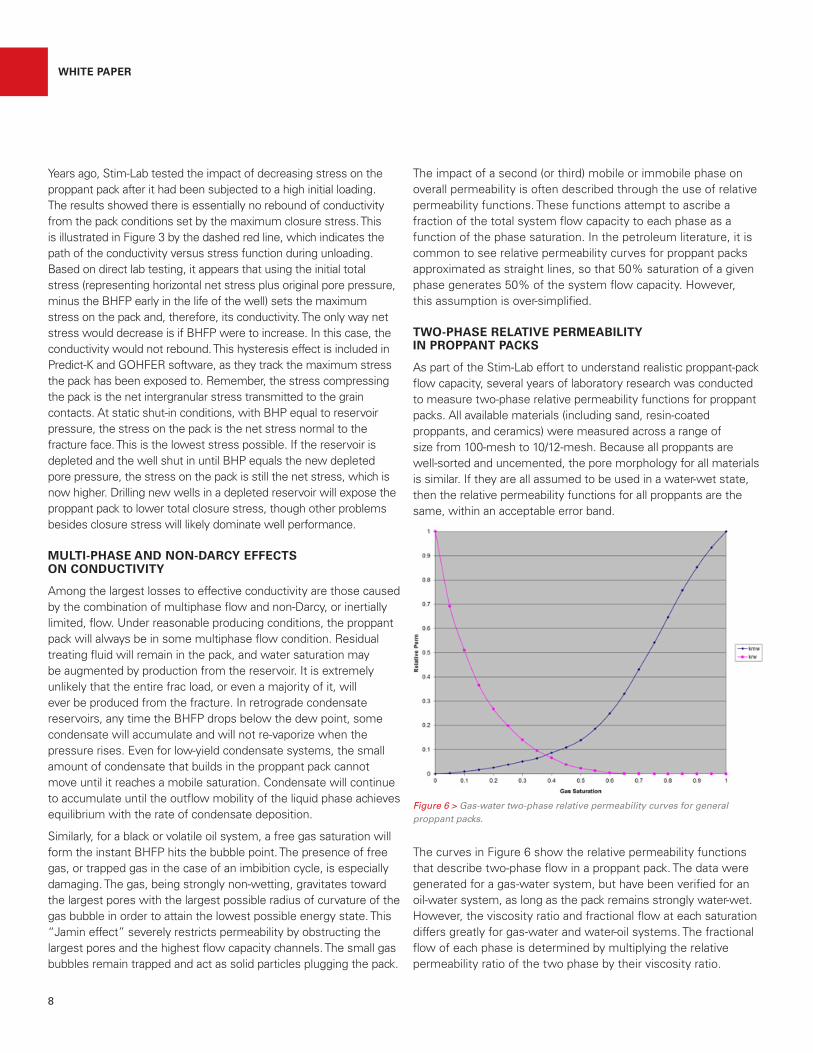
As part of the Stim-Lab effort to understand realistic proppant-pack flow capacity, several years of laboratory research was conducted to measure two-phase relative permeability functions for proppant packs. All available materials (including sand, resin-coated proppants, and ceramics) were measured across a range of size from 100-mesh to 10/12-mesh. Because all proppants are well-sorted and uncemented, the pore morphology for all materials is similar. If they are all assumed to be used in a water-wet state, then the relative permeability functions for all proppants are the same, within an acceptable error band.

The curves in Figure 6 show the relative permeability functions that describe two-phase flow in a proppant pack. The data were generated for a gas-water system, but have been verified for an oil-water system, as long as the pack remains strongly water-wet. However, the viscosity ratio and fractional flow at each saturation differs greatly for gas-water and water-oil systems. The fractional flow of each phase is determined by multiplying the relative permeability ratio of the two phase by their viscosity ratio.

Figure 6 > Gas-water two-phase relative permeability curves for general proppant packs.

WHITE PAPER

8

For example, at roughly 40% gas saturation, for an oil/water viscosity ratio near 1, the two phases would each exhibit roughly 50% fractional flow, though each phase would have a permeability that is only 9% of the absolute permeability of the pack. For a gas/water viscosity ratio of 50, at the same saturation, the gas fractional flow would be 98% of the flow stream with only 2% water moving.

The wetting phase and non-wetting phase relative permeability functions can be approximated using Corey functions. Taking water saturation (Sw) as a fraction, the wetting phase relative permeability is approximately Sw^5.5. The non-wetting phase permeability is approximately (1-Sw)^2.7.

Caution is required when using these functions to model fracture flow and cleanup. For flow to be governed by relative permeability, the flow conditions must be dominated by viscous forces. Capillary and gravity forces must be negligible, and saturation and flow capacity cannot be impacted by “capillary-end effects,” or discontinuities in the porous medium. These conditions are commonly used in simulations, though they rarely occur in real fractured reservoirs. To correctly measure the proppant pack relative permeability curves during laboratory testing, it was necessary to construct 20-ft-long proppant packs so that the length of the pack dominated by the capillary outlet discontinuity did not affect the results. A high flow rate was also needed to obtain stable pressure differentials. The subsequent rate was high enough to exceed the Darcy flow regime limits, so the observed relations between rate, pressure gradient, and saturation then had to be corrected for inertial effects.

NON-DARCY OR INERTIAL EFFECTS ON CONDUCTIVITY

Non-Darcy flow, or inertial effects, can be described for all proppants, using a single dimensionless flow model that was developed at Stim-Lab after extensive testing on multiple proppant types and over a large range of stresses, including mechanically damaged, or “crushed,” proppant. The final function describing inertial flow is shown in Figure 7. The original publication of this work is SPE 89325.

The y-axis shows the fraction of the Darcy permeability remaining as flowing Reynolds number increases. Reynolds number is given by (ρ*v)/(μ*Τ), where Τ can be determined as the inverse of the correct β*k, the value of (ρ*v)/μ at which the observed permeability is half the Darcy permeability, or 1/2D, where D is the median particle size of the proppant sieve distribution (in centimeters). The two exponents (F and E) were found to have values of slightly less than 1, and the minimum permeability (kmin) was proven but may be impossible to reach under any realistic flow conditions. This function applies for single-phase flow in a proppant pack. When more than one phase is present, the combined effects of multiphase flow and inertial effects are much more severe.

A second phase decreases the available pore channels of the non-wetting phase that are open to flow. This increases its velocity and Reynolds number, and reduces flow capacity. The wetting and non-wetting phases move through different pore channels at different speeds, and, therefore, each has its own effective Reynolds number and inertial resistance. The extension to multiphase non-Darcy flow is presented in SPE 109561. Some of the laboratory results, shown in Figure 8, show that the interchange of relative permeability and inertial effects is complex. For instance, because of the different Reynolds number for each phase, flow at constant fractional flow leads to a different equilibrium saturation at each rate. This interaction leads to an apparent plateau in the flow capacity at a high Reynolds number, when both phases are mobile. The lines in the figure are predictions based on the model and the points are experimental observations.

The combined effects of multiphase and non-Darcy flow are the largest losses of conductivity in parts of the fracture subjected to high velocity. Under reasonable flowing conditions in a fractured completion in unconventional reservoirs, these factors can lead

Figure 7 > Generalized dimensionless function for non-Darcy inertially influenced flow in a proppant pack.

Figure 8 > Non-Darcy flow for two phases at constant fractional flow across a range of Reynolds numbers.

WHITE PAPER

9

to about two orders of magnitude loss in fracture flow capacity. Considering no other damage mechanisms, these factors can also result in an apparent fracture conductivity that is 1% to 2% of the baseline value.

GEL CLEANUP AND RESERVOIR ENERGY

There are several issues associated with gel damage cleanup or removal from the proppant pack. The first is filter-cake deposition and removal. In unconventional reservoirs, where “matrix” permeability is extremely small, there will be little or no filter-cake deposition, and most leakoff will be associated with fissures and induced shear fractures. In very-high-permeability systems, above 500 mD, there will be almost no filter cake on the fracture wall, as polymer will invade the formation and generate leakoff control through invasion and pore obstruction. Most studies focus on the intermediate range of conventional reservoir permeability, where filter-cake deposition causes the most concern. The filter-cake deposition versus the logarithm of permeability is depicted as a bell-shaped curve, with a maximum at permeability of approximately 1 mD.

FILTER-CAKE DEPOSITION AND EROSION

Polymer concentration in a compressed filter cake is extremely high and cannot be dissolved or removed by breakers or high-velocity flow (erosion). Breakers generally allow the cake to compress, de-water, and become denser and more immobile. Under high hydrostatic pressure, the filter cake can compress while the total mass of polymer it contains remains constant. Upon release of the pressure differential, these cakes have been observed to re-imbibe water and to swell to fill all available pore space in the proppant pack. In general, if a gel residue concentration of more than 400 ppt exists in any part of the fracture, that portion of the pack is assumed to be fully plugged (as in Figure 2).

Given that filter cake is deposited while the fracture is held open by hydraulic pressure, it will change thickness during closure. For example, a cake of 0.01 in. compressed on the wall during pumping will extrude into the pore space of the proppant pack at closure. Assuming, for simplicity, that the proppant pack porosity is 33%, the thickness of the cake will triple upon complete closure. The resulting extruded cake, with a thickness of about 0.03 in., will “swallow” an entire 20/40-mesh proppant grain from each wall of the pack.

High-flow-rate tests, with brine flowing through the walls of the fracture and then through the pack, have shown that the filter cake cannot be removed. It is classified as a loss of flowing fracture width rather than a reduction in pack permeability. The remaining gel residue distributed throughout the pore space generates the remaining permeability damage.

POLYMER GEL RESIDUE AND DAMAGE

Cleanup of the distributed gel residue in the pack has been related to the amount of energy that can be transmitted to the gel by the flowing fluid stream. Figure 9 shows the data for several fluids and the model curve for percent regained permeability, relative to the absolute permeability of the pack, as a function of pseudo-Reynolds number (pRe). The term rho*v/mu is not dimensionless, as it is missing the effective diameter of the pore system.

The fluid represented by the magenta line has a maximum regained permeability of 90% of the absolute permeability of a clean pack. To achieve that degree of cleanup, the reservoir must be capable of developing a pRe of more than 30. If the reservoir permeability, pore pressure, or applied drawdown is too low, the reservoir may have insufficient energy to reach a high enough pRe. In the Figure 9 example, a reservoir that can only develop enough flow to get to pRe=0.5 will generate less than 10% cleanup of a fluid that could be capable of 90% cleanup under ideal conditions.

For cases of high-gel-residue concentration, approaching a gel plug, it is necessary to also consider the minimum pressure differential required to initiate flow, as shown in Figure 2. A gel plug behaves as if it has a substantial yield point, like a Bingham plastic fluid. If a sufficient potential gradient is not available, the gel will not move. In either case, it is the reservoir that is responsible for cleanup and development of effective fracture length, not primarily the fracture itself.

An extreme example of this is a 2-lb/ft2 propped fracture containing 20/40-mesh sintered bauxite, at only 2,000-psi closure stress, with a propped length of 1,000 ft, covering the entire reservoir thickness uniformly, placed with water and containing no gel residue or filter cake. While this may sound ideal, it raises the following questions: What is the effective producing length? What if the imaginary reservoir has zero porosity and zero permeability? With no flow through the “perfect” fracture, what is its effective length?

Figure 9 > Current gel cleanup model, with regained permeability as a function of pseudo-Reynolds number established in the fracture.

WHITE PAPER

10

VELOCITY AND POTENTIAL GRADIENTS DURING PRODUCTION AND CLEANUP

So, cleanup and effective fracture length depend on the coupling between the fracture and reservoir. The reservoir flow capacity provides the energy to drive cleanup and develop effective length. With insufficient energy, there will be little conductivity development. At the end of the fracture treatment, the proppant pack and surrounding fracture walls will be at essentially 100% water saturation, with no hydrocarbon flow capacity. Initial invasion of the water-saturated pack and penetration of the capillary blockage at the fracture wall will be discussed in the next section. But first, the velocity and potential gradient generated during typical producing conditions must be considered. Understanding of the relative magnitude of viscous, capillary, and gravity forces requires quantification of the various potential gradients.

CONVERGENT SKIN EFFECTS FOR HORIZONTAL WELLS

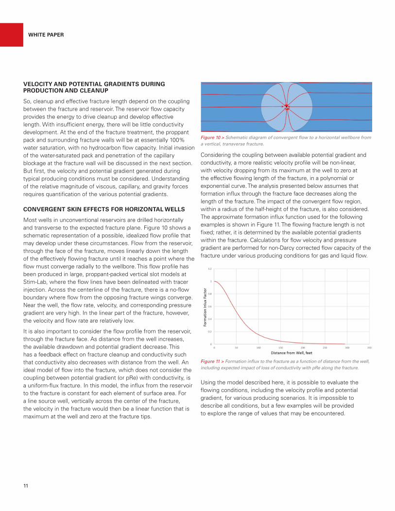
Most wells in unconventional reservoirs are drilled horizontally and transverse to the expected fracture plane. Figure 10 shows a schematic representation of a possible, idealized flow profile that may develop under these circumstances. Flow from the reservoir, through the face of the fracture, moves linearly down the length of the effectively flowing fracture until it reaches a point where the flow must converge radially to the wellbore. This flow profile has been produced in large, proppant-packed vertical slot models at Stim-Lab, where the flow lines have been delineated with tracer injection. Across the centerline of the fracture, there is a no-flow boundary where flow from the opposing fracture wings converge. Near the well, the flow rate, velocity, and corresponding pressure gradient are very high. In the linear part of the fracture, however, the velocity and flow rate are relatively low.

It is also important to consider the flow profile from the reservoir, through the fracture face. As distance from the well increases, the available drawdown and potential gradient decrease. This has a feedback effect on fracture cleanup and conductivity such that conductivity also decreases with distance from the well. An ideal model of flow into the fracture, which does not consider the coupling between potential gradient (or pRe) with conductivity, is a uniform-flux fracture. In this model, the influx from the reservoir to the fracture is constant for each element of surface area. For a line source well, vertically across the center of the fracture, the velocity in the fracture would then be a linear function that is maximum at the well and zero at the fracture tips.

Considering the coupling between available potential gradient and conductivity, a more realistic velocity profile will be non-linear, with velocity dropping from its maximum at the well to zero at the effective flowing length of the fracture, in a polynomial or exponential curve. The analysis presented below assumes that formation influx through the fracture face decreases along the length of the fracture. The impact of the convergent flow region, within a radius of the half-height of the fracture, is also considered. The approximate formation influx function used for the following examples is shown in Figure 11. The flowing fracture length is not fixed; rather, it is determined by the available potential gradients within the fracture. Calculations for flow velocity and pressure gradient are performed for non-Darcy corrected flow capacity of the fracture under various producing conditions for gas and liquid flow.

Using the model described here, it is possible to evaluate the flowing conditions, including the velocity profile and potential gradient, for various producing scenarios. It is impossible to describe all conditions, but a few examples will be provided to explore the range of values that may be encountered.

Figure 10 > Schematic diagram of convergent flow to a horizontal wellbore from a vertical, transverse fracture.

Figure 11 > Formation influx to the fracture as a function of distance from the well, including expected impact of loss of conductivity with pRe along the fracture.

WHITE PAPER

11

EFFECTIVE CONDUCTIVITY IN OIL WELLS

The first example represents an oil well flowing at initial high-rate conditions while still above the bubble point in single-phase flow. The model was run to simulate a horizontal well with 30 active and contributing transverse fractures, each 50 ft tall. The produced fluid is assumed to have a viscosity of 1 cp. The initial rate from the well is 5,400 BOPD, which translates to 180 BOPD per fracture (90 BOPD per wing). Assuming an average proppant concentration of approximately 1 lb/ft2 (pack width of 0.1 in.) and an effective producing permeability (under Darcy conditions) of 10 darcies (83 mD-ft effective conductivity), the velocity and Reynolds number can be computed over the length of the fracture. These results are used to adjust the permeability for inertial effects in the convergent flow region. The resulting velocity profile and corresponding potential gradient are shown in Figure 12.

The pressure gradient at the wellbore sandface is 4,000 psi/ft, declining to 550 psi/ft only 1 ft from the well. This indicates that the well is likely physically limited to a lower initial rate by near-well tortuosity and convergent flow. At a distance of 100 ft from the well, the pressure gradient is approximately 2 psi/ft. Toward the tip of the fracture, as reservoir flux decreases, the pressure gradient rapidly drops. At 240 ft, the gradient is 0.18 psi/ft. Note that the average superficial flow velocity drops below 0.1 cm/sec to zero at less than 90 ft from the well. Beyond 300 ft of fracture half-length, the potential gradient drops rapidly below 0.1 psi/ft and enters the capillary dominated region.

Figure 13 illustrates the total pressure drop from the wellbore sandface along the fracture length. At 70 ft from the well, approximately 3,000 psi of the available drawdown is consumed.

The remaining 250 psi of total drawdown is consumed over the remaining fracture length. The gradient and velocity in the distal region of the fracture is so low that cleanup is problematic.

The same well and fracture conditions are shown in Figures 14 and 15 after the total well rate has declined to 190 BOPD. At this rate, each fracture produces 6.3 BOPD or approximately 12 oz/min – not enough to push water out of the fracture. The pressure gradient is less than 0.1 psi/ft from 100 ft to the tip of the fracture. At the wellbore, the gradient is about 40 psi/ft. Velocity drops below 0.03 cm/sec at only 10 ft from the well. At 100 ft, the velocity is 0.002 cm/sec. For mechanical cleanup to be achieved, it must occur early in the life of the well. Later accumulation of water in the extremities of the fracture will likely be impossible to move at these conditions.Figure 12 > Fluid velocity and potential gradient in a 50-ft-tall fracture with

1-lb/ft2 proppant, 83 mD-ft conductivity, 30 fractures, producing at 5,400 BOPD.

Figure 13 > Total pressure drop from the wellbore face, as a function of fracture length in a 50-ft-tall fracture with 1-lb/ft² proppant, 30 fractures, 83 mD-ft conductivity, producing at 5,400 BOPD.

Figure 14 > Fluid velocity and potential gradient in a 50-ft-tall fracture with 1-lb/ft2 proppant, 83 mD-ft conductivity, 30 fractures, producing at 190 BOPD.

WHITE PAPER

12

EFFECTIVE CONDUCTIVITY IN GAS WELLS

Using the same fracture geometry and conductivity, a gas well producing a 4.4 MMSCF/D at a BHFP of 3,000 psi was modeled using a gas viscosity of 0.02 cp. Single-phase flow was again assumed, but the Darcy conductivity was held at 83 mD-ft. The potential gradient and velocity are shown in Figure 16 for the initial production rate.

The high gas mobility actually has a negative impact on cleanup potential and a much higher non-Darcy flow effect. The pressure gradient at the well is approximately 3,000 psi/ft, but drops to 4 psi/ft only 10 ft from the well. Over the bulk of the fracture length, at distances of 50 ft to 100 ft, the pressure gradient is 0.4 psi/ft to 0.06 psi/ft, or typically less than the gas-water gravity head. From

100 ft to the tip of the fracture, the viscous gradient is far below the gravity head.

Velocity drops from 23 cm/sec at the sandface to 0.8 cm/sec 10 ft from the well. Over the rest of the fracture, the velocity drops from 0.2 cm/sec at 50 ft to less than half that at 100 ft, and approaches zero beyond 300 ft. Subsequently, meaningful flow or indication of an “effective” fracture contribution from most of the fracture is unlikely.

The overall pressure drop for the high-rate gas well is shown in Figure 17. Note that almost the entire pressure drawdown is consumed within the first 10 ft of the well. Very little energy is left over the bulk of the fracture to aid in cleanup or water removal.

Once the gas well declines to about 150 MMSCF/D (a comparable in-situ velocity to the oil case), the energy in the fracture is greatly diminished. Figures 18 and 19 depict the conditions in the fracture for the depleted gas well. Potential gradients are less than the gas-water gravity head at less than 5 ft from the well. Note that the potential gradient is less than 0.03 psi/ft at only 10 ft from the well – a value that will be of significance during the discussion on capillary phenomena.

Superficial gas velocity in the fracture is less than 1 cm/sec at the well and below 0.1 cm/sec at less than 3 ft. The velocity is less than 0.03 cm/sec at a distance beyond 10 ft, and less than 0.01 cm/sec beyond 50 ft.

The overall total pressure drop through the whole fracture (Figure 19) is less than 3 psi over 300 ft, with 2 psi over the first 12 ft. If liquids accumulate in the proppant pack under these conditions, there is virtually no way to remove them by displacement.

Figure 15 > Total pressure drop from the wellbore face, as a function of fracture length in a 50-ft-tall fracture with 1-lb/ft² proppant, 30 fractures, 83 mD-ft conductivity, producing at 190 BOPD.

Figure 17 > Total pressure drop from the wellbore face, as a function of fracture length, in a 50-ft-tall fracture with 1-lb/ft² proppant, 30 fractures, 83 mD-ft conductivity, producing at 4.4 MMSCF/D dry gas.

Figure 16 > Fluid velocity and potential gradient in a 50-ft-tall fracture with 1-lb/ft² proppant, 83 mD-ft conductivity, 30 fractures, producing at 4.4 MMSCF/D dry gas.

WHITE PAPER

13

DEGRADATION OF PROPPANT CONDUCTIVITY OVER TIME

The Stim-Lab “baseline” conductivity data are taken at 50 hr of flow at each stress. Analysis of the data shows that the pack conductivity is relatively unstable at 50 hr, even under ideal laboratory conditions using mineral-saturated, deoxygenated brine. Figure 20 presents data for a particular proppant, with observed conductivity versus time normalized to the conductivity after 1 hr at stress.

At high stress (about 10,000 psi), the proppant shown has lost approximately 25% of the conductivity observed after 1 hr, for only 50 hr at stress. Additional testing has provided no indication that conductivity ever stabilizes, regardless of the flow time. Reasons for this continued degradation are still debated, but likely include long-term creep, pressure solution and precipitation of silica, and degradation of the substrate rock surface. Figure 21 shows an illustration from the ASME Journal of Energy Resources Technology, which demonstrates the effect of time, creep, pressure solution, and precipitation in a proppant pack. However, the rate of degradation in the field is expected to be much more severe. These tests do not represent the cumulative effects of scale deposition, salt plugging, fines migration from the reservoir, deposition of waxes and asphaltenes, bacterial slime, and other probable progressive damage that occur during production.

Figure 18 > Fluid velocity and potential gradient in a 50-ft-tall fracture with 1-lb/ft² proppant, 83 mD-ft conductivity, 30 fractures, producing at 150 MMSCF/D dry gas.

Figure 19 > Total pressure drop from the wellbore face, as a function of fracture length, in a 50-ft-tall fracture with 1-lb/ft² proppant, 30 fractures, 83 mD-ft conductivity, producing at 150 MMSCF/D dry gas.

Figure 20 > Time-dependent proppant pack conductivity under ideal laboratory conditions.

Figure 21 > Time-dependent degradation of proppant pack due to solution and re-precipitation of minerals.

WHITE PAPER

14

Given that the proppant pack is essentially a fixed sand-bed filter between the reservoir and the well, plugging and damage are expected to accumulate over time. As a result, the fracture conductivity will have a finite life that can be measured in months. Extrapolation of early time production to 20 yr or more to justify stimulation costs is probably not a justifiable practice, since the fracture will likely have little or no useful conductivity at that time. Due to the reservoir transient behavior, there will, fortunately, be so little fluid moving through the fracture in late time that conductivity is no longer a limiting constraint on the well’s productivity.

CAPILLARY AND GRAVITY FORCES

In the above cases, a formation influx factor was assumed with decreasing influx away from the well. While overall results are not strongly sensitive to the shape of this function, details may change. Based on all the available laboratory data, it is possible that cleanup and conductivity may suffer significantly at very low potential gradients and low values of pRe. In these examples, it is difficult to justify much flow beyond a few hundred feet of fracture length. The gross created fracture length could be 1,000 ft or more, but, beyond a couple hundred feet, there is insufficient energy to overcome gravity and capillary forces in the proppant pack. This limits the total flowing length of the fracture based on reservoir energy.

In the absence of gel damage (i.e., filter cake), there are still alternative damage mechanisms that can stop hydrocarbon movement in the proppant pack. These are related to the capillary forces at the filtrate-invaded fracture wall and in the proppant pack itself. At the end of the fracture treatment, the proppant pack is 100% water-saturated and the fracture wall has been invaded with fluid filtrate, forced in under (typically) more than 1,000 psi pressure differential. Capillary forces in both these regions may block or limit movement of a non-wetting hydrocarbon phase.

DERIVATION OF CAPILLARY ENTRY PRESSURE

This section examines the capillary blockage (i.e., end effect) that occurs at the interface between the formation fracture face and proppant pack. The pore size within the pack is so large, compared to the pore size of the formation, that a capillary pressure discontinuity will exist at every fracture surface. The source of the capillary discontinuity is the phase pressure differential caused by the radius of curvature of the interface between two immiscible fluids. The common definition of the phase pressure differential across a distended interface, or capillary pressure, is derived in the equations provided in Figure 22.

In the equations, σ is the interfacial tension (IFT) between the two phases (dynes/cm). The wetting phase contact angle with the solid surface is given by θ. The radius of the capillary is r and represents

the radius of the reservoir or proppant pack pore throat. A typical water-oil system will have an interfacial tension of 20 to 30 dynes/cm, while a gas-water system will typically be in the range of 50 to 70 dynes/cm. Use of effective surfactants may drop interfacial tension to about 5 dynes/cm. A purely water-wet system will have a contact angle approaching zero, with Cos(θ)=1. Intermediate or neutrally wet systems may have contact angles of 60° to 90°. If a contact angle of 90° were possible, there would be no capillary phase pressure differences between the phases.

CAPILLARY ENTRY PRESSURE FOR SHALE AND TIGHT-SAND RESERVOIRS

The pore size of typical reservoir rocks, r, is provided in Figure 23 (Nelson, AAPG Bulletin 93, No. 3, March 2009). Note that unconventional systems, typically shale, have a pore diameter ranging from 0.01 to 0.1 microns, while “tight” gas sands typically range from 0.05 to 1 micron.

Figure 22 > Explanation and derivation of the conventional capillary pressure equation.

Figure 23 > Pore diameter for typical petroleum reservoir rocks.

WHITE PAPER

15

These values can be used to estimate the capillary threshold pressure for a range of contact angles and pore sizes that may be encountered along the face of a fracture. Figure 23 shows the results of these calculations for the following scenarios: a contact angle of zero and IFT of 70 dynes/cm (gas-water), zero contact angle and IFT=30 (gas-oil), a contact angle of zero and surfactant-reduced IFT of 5 dynes/com (surf), and a contact angle increased to 85° to represent a strongly oil-wet system (e.g., organic-rich shale source-rock).

Note that, for water-wet shales (pore sizes of 0.005 to 0.05 micron diameters), the threshold entry pressure is more than 1,000 psi. This means that the invaded face of the fracture forms a capillary wall that must be breached to move the non-wetting (hydrocarbon) phase from the reservoir to the proppant pack. This capillary blockage will exist even if the invaded zone is only a few pore diameters in thickness. This capillary threshold pressure, or caprock seal capacity, can (and has been) measured in the laboratory for water-saturated shale samples. In some shale systems, a pressure differential greater than 1,000 psi is required to inject a single bubble or droplet of gas/oil into the shale. If the shale is oil-wet, and the produced phase is oil, then the threshold pressure may be much lower, as shown by the light blue curve (ca, in Figure 24).

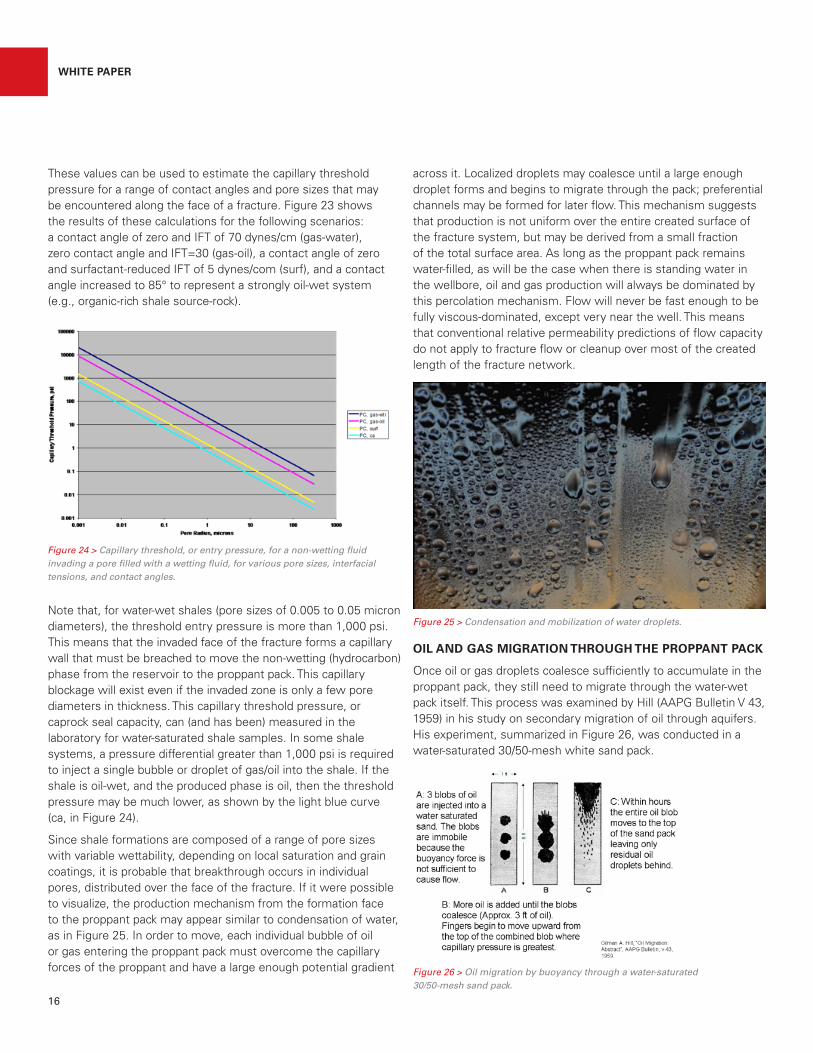
Since shale formations are composed of a range of pore sizes with variable wettability, depending on local saturation and grain coatings, it is probable that breakthrough occurs in individual pores, distributed over the face of the fracture. If it were possible to visualize, the production mechanism from the formation face to the proppant pack may appear similar to condensation of water, as in Figure 25. In order to move, each individual bubble of oil or gas entering the proppant pack must overcome the capillary forces of the proppant and have a large enough potential gradient

across it. Localized droplets may coalesce until a large enough droplet forms and begins to migrate through the pack; preferential channels may be formed for later flow. This mechanism suggests that production is not uniform over the entire created surface of the fracture system, but may be derived from a small fraction of the total surface area. As long as the proppant pack remains water-filled, as will be the case when there is standing water in the wellbore, oil and gas production will always be dominated by this percolation mechanism. Flow will never be fast enough to be fully viscous-dominated, except very near the well. This means that conventional relative permeability predictions of flow capacity do not apply to fracture flow or cleanup over most of the created length of the fracture network.

OIL AND GAS MIGRATION THROUGH THE PROPPANT PACK

Once oil or gas droplets coalesce sufficiently to accumulate in the proppant pack, they still need to migrate through the water-wet pack itself. This process was examined by Hill (AAPG Bulletin V 43, 1959) in his study on secondary migration of oil through aquifers. His experiment, summarized in Figure 26, was conducted in a water-saturated 30/50-mesh white sand pack.

Figure 24 > Capillary threshold, or entry pressure, for a non-wetting fluid invading a pore filled with a wetting fluid, for various pore sizes, interfacial tensions, and contact angles.

Figure 25 > Condensation and mobilization of water droplets.

Figure 26 > Oil migration by buoyancy through a water-saturated 30/50-mesh sand pack.

WHITE PAPER

16

In panel A, there are three disconnected droplets of oil, each approximately 4 in. in diameter, which were injected by syringe into the water-saturated sand pack. The buoyancy force created by the height of each droplet, fluid density difference, and gravitational acceleration is insufficient to overcome the threshold pressure of the pack. The oil cannot move under a potential gradient of about 0.09 psi/ft (assuming an oil-water density difference of 0.2 g/cm3). Water permeability through the pack is in the range of hundreds of darcies, and may add some hydrodynamic gradient to the oil droplets at a high water flow rate.

As depicted in panel B, the oil droplets gradually increase in size through additional oil injection until the total continuous height of the oil is approximately 36 in. At this point, the buoyant force at the top leading edge of the oil drop reaches the threshold pressure of the water-filled pores in the pack. This is an approximate phase pressure difference of 0.26 psi at the limiting pore throats. Once the threshold pressure is breached, the entire oil blob (or ganglion) migrates upward through the pack. Water displaced by the moving oil falls around the oil and fills in the pore space. Net “load recovery” is effectively zero during this migration, or percolation, of the oil. The area vacated by the oil now contains residual trapped oil droplets that may act to block pores and reduce pack permeability, and could be hard to contact and mobilize by later produced oil ganglia.

This experiment may describe the common producing process that occurs over much of the fracture system. In typical well operations, the pump or tubing tail is set high enough above the lateral that the horizontal section of the well maintains a water layer. Any fractures that have a continuous source of water, aided by gravity drainage, will tend to remain water-filled, with local percolation of gas and oil droplets moving through the proppant pack.

CAPILLARY ENTRY PRESSURE OF PROPPANT PACKS FOR VARIOUS SIEVES

As a result of these observations, Stim-Lab measured the capillary threshold pressure of typical water-wet proppant packs of various sizes. The data were compared with theoretical calculations of entry pressure, based on expected pore size derived from sieve distributions. The results of these measurements are summarized in Figure 27. The oval centered at the 40-mesh size shows an entry pressure of approximately 0.26 psi, which corresponds to the set conditions of the Hill experiment. For this sand pack, an oil droplet of roughly 36 in. in height is needed to achieve mobility through buoyancy. A gas bubble about 8 in. in height could achieve mobility in the same pack.

Referring back to Figures 12 through 19, the estimated potential gradient at various flow conditions can be compared to the gravity head for gas-oil and oil-water systems. At a very high flow rate, usually early in the life of the well, the viscous gradient may equal or exceed the gravity potential gradient at a distance of more than 100 ft from the well. Unfortunately, the water saturation in the pack is at a maximum at this time, and oil and gas mobility may be limited. After the initial hyperbolic decline period in the low-rate case, the gravity head dominated the viscous gradient several feet to tens of feet from the well. Over much of the producing life of the well, and over most of the fracture length, gravity and capillary forces control oil and gas migration, not viscous forces, and, therefore, are not relative permeability functions.

FLOW REGIMES IN VERTICAL TRANSVERSE FRACTURES

If gravity drainage is an important part of fracture cleanup and conductivity, the geometry of a transverse fracture on a horizontal well must be considered more carefully. Figure 28 is a hypothetical illustration of a vertical transverse fracture on a horizontal well intersecting the center of the fracture height. Three different flow regimes are represented, each with a different potential for developing conductivity and contributing to production.

Figure 27 > Capillary entry, or threshold pressure, for water-wet proppant packs, based on mean sieve size of the particles in the pack.

WHITE PAPER

17

In the upper part of the fracture, the proppant pack will drain effectively by gravity. The water saturation left behind by the fracturing fluid will drop to approximately the capillary residual saturation (10% to 15%), and the high gas and oil saturation will enable substantial flow capacity to those phases. The water saturation at the face of the fracture will continue to decrease over time through production, gravity drainage, and spontaneous imbibition into the reservoir. This section of the fracture, if allowed to drain, will provide the most efficient stimulation and effective flow area.

The section of the fracture below the lateral is in a disadvantaged state, where water saturation will be constantly replenished by any water flowing down the wellbore and gravity draining into the fracture. As long as there is some water production from the well, these fracture segments will probably remain waterlogged. Oil and gas can only migrate through the water-saturated proppant pack by percolation, and the fracture faces will remain at a high water saturation, with severe capillary blockage. It is possible that the flow rates in these lower fracture limbs will be so small that they will not affect the transient production of the well and may not contribute to producing net pay thickness.

The third flow regime is the convergent area around the well, where potential gradients and velocities are high. This area will be dominated by inertial losses and viscous forces, and will likely be in a constant multiphase flow condition. The calculations presented in Figures 12 through 19 clearly demonstrate the impact of this region.

EFFECTIVE FRACTURE LENGTH AND DIMENSIONLESS CONDUCTIVITY

Integrating the potential damage mechanisms is a complex and dynamic process that changes continuously during the producing history of the well. Gel and filter-cake damage removal, which may occur early in the well’s life while high pRe flow conditions are possible, is assumed to persist through the life of the well. Long-term progressive conductivity damage will also continue to increase throughout the well’s life. On the other hand, saturation effects are transient and may come and go rapidly in response to changes in well operating conditions such as pump efficiency, tubing setting depth, applied drawdown, reservoir pressure depletion, and reservoir transient response. These effects – which are also related to well loading and cyclic shut-in or killing operations, including well bashing from offset well stimulation – offer the greatest potential for damage and loss of effective fracture conductivity.

RESATURATION AND HYSTERESIS EFFECTS

Another potential damage mechanism is water imbibition from shut-ins, well killing, or bashing. The proppant pack conductivity will be impacted by successive drainage and imbibition cycles, causing a change in direction from decreasing to increasing wetting phase saturation. This is illustrated in Figure 29, which shows both primary drainage and imbibition cycles for a gas-water system in a reservoir core sample.

Figure 28 > Diagram of possible flow regimes in a vertical transverse fracture on a horizontal well.

Figure 29 > Drainage and imbibition cycle relative permeability curves for a reservoir core sample.

WHITE PAPER

18

The same trend is present in proppant packs. On primary drainage (initial cleanup), the wetting phase (frac load) saturation decreases and gas or oil permeability increases. If water is reintroduced into the pack as a result of a shut-in, secondary injection, or influx from an offset fracture treatment, the water saturation increases rapidly due to the favorable mobility ratio of water displacing oil or gas. The water influx leaves a trapped non-wetting phase saturation in the pore space, or lack thereof, that is discontinuous and effectively impossible to move by later drainage cycles. This cuts the maximum attainable permeability of the system, even at 100% fractional flow of a single phase, by up to 80% in many cases. Later drainage and imbibition cycles operate within a reduced hysteresis loop on the saturation-relative permeability plot. If the waterflood occurs late in the life of the well, when there is little energy left in the system, the affected fractures may never recover useful flow capacity.

DIMENSIONLESS FRACTURE CONDUCTIVITY

Accounting for all potential damage mechanisms, at any time during the producing life of the well, makes it possible to estimate an effective proppant pack conductivity (kfwf ), usually expressed in units of mD-ft. This damaged effective dynamic conductivity is often used to compute a dimensionless fracture conductivity, FCD. The equation for FCD is shown as Eq. 2.

The effective producing permeability of the reservoir is shown as kr . By using this dimensionless conductivity, however, the flowing length of the fracture is not well defined and is essentially independent of the fracture conductivity alone. Throughout this discussion, it has been asserted that the length of fracture that can sustain flow depends heavily on the available flow capacity and energy of the reservoir. A high-conductivity fracture in an impermeable reservoir will have a high FCD but virtually no effective length. Through the Stim-Lab consortium, a model has been developed and implemented in the Predict-K and GOHFER software; this model estimates the flowing length based on the energy balance, pRe, and transient production from a given reservoir. That transient flowing length can then be used to derive a dimensionless conductivity that changes constantly, along with flowing length, through the life of the well.

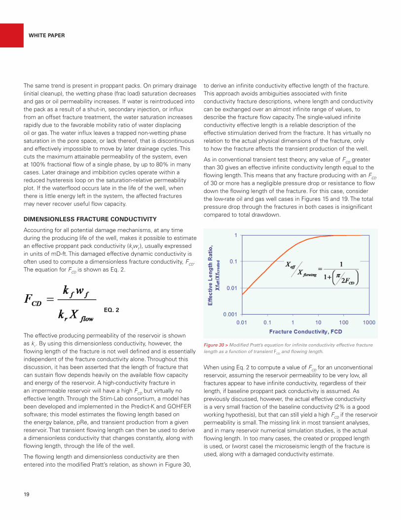
The flowing length and dimensionless conductivity are then entered into the modified Pratt’s relation, as shown in Figure 30,

to derive an infinite conductivity effective length of the fracture. This approach avoids ambiguities associated with finite conductivity fracture descriptions, where length and conductivity can be exchanged over an almost infinite range of values, to describe the fracture flow capacity. The single-valued infinite conductivity effective length is a reliable description of the effective stimulation derived from the fracture. It has virtually no relation to the actual physical dimensions of the fracture, only to how the fracture affects the transient production of the well.

As in conventional transient test theory, any value of FCD greater than 30 gives an effective infinite conductivity length equal to the flowing length. This means that any fracture producing with an FCD of 30 or more has a negligible pressure drop or resistance to flow down the flowing length of the fracture. For this case, consider the low-rate oil and gas well cases in Figures 15 and 19. The total pressure drop through the fractures in both cases is insignificant compared to total drawdown.

When using Eq. 2 to compute a value of FCD for an unconventional reservoir, assuming the reservoir permeability to be very low, all fractures appear to have infinite conductivity, regardless of their length, if baseline proppant pack conductivity is assumed. As previously discussed, however, the actual effective conductivity is a very small fraction of the baseline conductivity (2% is a good working hypothesis), but that can still yield a high FCD if the reservoir permeability is small. The missing link in most transient analyses, and in many reservoir numerical simulation studies, is the actual flowing length. In too many cases, the created or propped length is used, or (worst case) the microseismic length of the fracture is used, along with a damaged conductivity estimate.

EQ. 2

Figure 30 > Modified Pratt’s equation for infinite conductivity effective fracture length as a function of transient FCD and flowing length.

WHITE PAPER

19

PROBLEMS WITH DIMENSIONLESS CONDUCTIVITY AND THE McGUIRE-SIKORA CURVES

The main problem with relative, or dimensionless, conductivity is illustrated by the McGuire-Sikora “folds of increase” curves, shown in Figure 31. In these curves, productivity increase is plotted along the ordinate with a correction for well drainage area, A. The stimulation ratio is J/Jo, or the expected folds-of-increase in productivity index resulting from the fracture.

The abscissa is a measure of the relative conductivity of the fracture to the surrounding formation, corrected for well spacing. Note that the fracture conductivity is used in units of mD-in., rather than the usual mD-ft, and that reservoir permeability is in mD. Well drainage area (A) is in acres. Fracture length is shown by the various curves as a function of fracture half-length relative to the well drainage radius.

These curves indicate that, for fractures with a low dimensionless conductivity (left end of the plot), a significant increase in fracture length will not improve productivity. For higher conductivity fractures, relative to the producing capacity of the formation (right side of the plot), this model predicts that increasing length can greatly improve the well productivity. For unconventional reservoirs, when using the often-measured crushed-core permeability, fractures tend to fall toward the right end of the plot. This suggests that conductivity is unimportant, and longer created fractures will always improve production.

There are several fallacies in this conclusion. The model assumes that the entire created fracture length represents the effective flowing length of the fracture. The model was derived for single-phase flow using an electrical analog model, and, therefore, capillary forces and cleanup are not recognized. In reality, it is impossible to clean up an extremely long fracture in a very-low-energy or flow-capacity reservoir. In unconventional reservoirs, the upper-right quadrant of the plot in Figure 31 effectively does not exist.

EFFECTIVE FLOWING LENGTH

When the low-energy state generated by production from an unconventional reservoir is considered, the flowing length can become severely limited – not by lack of conductivity, but by lack of reservoir energy. Combining the energy available to drive cleanup with the dynamic conductivity of the overall fracture system, it is possible to estimate the effective infinite conductivity fracture length that can result. This length can be used to predict the production and decline profile of a well, and help to optimize fracture treatment design. Figure 32 presents an example of this process, as described in SPE 84306 and 84491.

The case modeled is a 1,000-ft propped fracture. Each curve on the plot represents damaged fracture conductivity, shown by the legend as “C”, where the values are in mD-ft. The x-axis is the producing reservoir effective permeability. The y-axis is the infinite conductivity fracture length, including cleanup response and dimensionless conductivity.

In very-high-permeability systems, the fracture conductivity is not sufficient to carry fluid from the reservoir to the well without a significant pressure drop. This is similar to the high-rate oil case of Figures 12 through 13. Non-Darcy inertial effects and the high velocity in the fracture diminish effective conductivity so that the FCD limit reduces the effective length. At the far right edge of the plot (1,000 mD reservoir permeability), with a 5,000-mD-ft proppant pack conductivity and 1,000-ft propped length, FCD is 0.005. According to the data in Figure 30, the effective fracture length will measure approximately 2 ft. This condition is commonly observed in offshore frac-pack completions.

At the left edge of the plot, a different condition exists. Reservoir permeability is less than 0.001 mD, so FCD for the fracture is greater than 30 and all fractures behave as infinite conductivity.

Figure 32 > Infinite conductivity effective length for a 1,000-ft propped fracture of various dynamic conductivities, producing from reservoirs of various permeability at fixed drawdown.

Figure 31 > McGuire-Sikora “folds of Increase” curves for pseudo-steady-state production, based on relative fracture conductivity.

WHITE PAPER

20

The limit is the cleanup of the fracture due to lack of reservoir energy. A sub-microdarcy reservoir will produce little flow rate, velocity, or potential gradient in the fracture. It will be difficult to achieve significant cleanup, so conductivity will be impaired. The low energy and low cleanup result in a short flowing length, though the entire available flowing length has a negligible pressure drop – hence, infinite conductivity. The lack of the pressure gradient is, itself, responsible for the poor effective fracture length.

The concept of FCD alone does not effectively describe fracture flow behavior without the additional constraint that extremely low-permeability reservoirs are not capable of cleaning up long fractures. Capillary and gravity forces dominate the fluid movement to such an extent that viscous gradients are negligible. This is equivalent, in the Hill experiment, of trying to flow oil through the water-saturated 30/50-mesh sandpack at an imposed differential pressure of 0.1 psi. Since the entry pressure is approximately 0.26 psi, it is possible for a proppant pack at 100% water saturation, with an absolute permeability to water of hundreds of darcies, to exhibit zero flow when oil is exposed to the inlet face of the pack with a pressure differential below the threshold.

In the middle range of Figure 32, the flow capacity of the reservoir and possible conductivity of the proppant pack are balanced for optimum performance. Long infinite-conductivity effective length fractures can be produced in this range of reservoir properties. Since the curves shown in the figure represent one drawdown condition, it should be remembered that high reservoir pressure and/or high drawdown can shift the curves to better performance at lower permeability. The converse is also true. Low-pressure reservoirs will not clean up as well, so the family of curves will shift to the right.

As usual, other factors affect well performance besides those that directly impact fracture conductivity. For example, highly over-pressured reservoirs may seem to offer the opportunity for high cleanup and high initial rate by pulling the well as hard as possible early in its life. However, a high pore pressure implies a low-net-effective stress in the reservoir, and the strong possibility of irreversible stress-dependent reservoir permeability. High drawdown for initial production may collapse the reservoir in the low-pore-pressure field around the well, causing the closure of microfractures and loss of reservoir flow capacity that will adversely affect all future production. In most cases, this stress-sensitive permeability collapse is not reversible even if the well is later constrained to allow BHFP to rise.

Similarly, water coning, or dropping below phase transition pressure (dew point or bubble point) early in the well life can have an irreversible and catastrophic impact on fracture conductivity. The entire well, fracture, and reservoir system must be taken as a tightly coupled system to determine the most effective stimulation design and well operating procedures. For most horizontal well

developments in unconventional reservoirs, there is a high chance that the primary issues are related to well operations rather than fracture geometry, proppant placement, proppant crush, or embedment. Current practices do not favor unloading of the well and fractures or removal of water, gravity-assisted drainage, and do not provide sufficient potential gradient to allow adequate cleanup of the existing fractures emplaced with current technology.

PROPPANT CUTOFF LENGTH, FLOWING LENGTH, AND EFFECTIVE LENGTH IN GOHFER SOFTWARE

GOHFER software strives to incorporate all previously discussed factors to determine a realistic effective fracture length, modeling as an infinite conductivity fracture, to be able to effectively compare different designs. The use of multiple fracture length descriptions (e.g., proppant cutoff length, flowing length, and effective length) often confuses users. The following discussion clarifies each definition, so they can be used accurately and consistently. Figure 33 shows an example output file generated by GOHFER software for each type of fracture length. The name of the “design” level in the GOHFER project is used, with a .csv file extension, to contain the data shown. The file resides in the top level of the design folder, under the appropriate geologic section.

For a given fracture treatment design, GOHFER outputs a grid of the vertical and lateral proppant concentration distribution. The mass/area concentration of the proppant in the fracture is used to compute the fracture width at closure. Local variations in total closure stress, formation modulus, filter-cake residue, compression of the proppant pack, and other factors are included in the estimate of flowing fracture width. The width and compressed pack conductivity, under the appropriate stress, are used to estimate a conductivity, in mD-ft, for each column of nodes (vertically) across the net pay covered by the fracture. The average proppant concentration with distance along the fracture is plotted in Figure 33 (line with blue diamonds), referring to the right ordinate axis.

Figure 33 > Output of various predicted fracture lengths (e.g., cutoff, flowing, and effective) from the GOHFER® software simulator.

WHITE PAPER

21

At this time, at the end of the fracture simulation, details about producing gas/oil ratio (GOR), gas/liquid ratio (GLR), and water cut are not available to the simulator, and, therefore, an estimate of multiphase flow effects is applied to the estimated proppant conductivity. The approximate conductivity as a function of length is plotted as the solid orange line. As fracture length increases and average concentration decreases, the average conductivity over the entire fracture declines.

The average conductivity, producing length, and average permeability from the model grid are used to estimate a flowing length of the fracture, using the cleanup algorithm presented previously. The estimated fracture length that can clean up and contribute flow is called the “flowing length,” and is plotted as the solid red line relative to the left ordinate axis. The flowing length and conductivity are used to compute the dimensionless conductivity (FCD as a function of fracture length, which is plotted as the solid yellow line). Finally, the FCD and flowing length are used to compute an approximate infinite conductivity effective length of the fracture, which is plotted as the solid blue line.

All estimates are established before production analysis or forecast simulations. The results are output in the design level summary table in the GOHFER output, along with the gross created fracture length, which is the maximum length of the fracture, propped or not, and also the largest value on the abscissa of the plot in Figure 33. Note that, for a proppant cutoff length of less than 200 ft to more than 1,900 ft, the predicted effective fracture length varies by less than 3 ft and averages 50 ft. The actual proppant cutoff length is an input to the production analysis and has no real value in describing the fracture. It can be used as an estimate of the effectively propped length, though the gross length of the fracture, which controls pressure hits on offset wells, is closer to the gross length. The length of fracture between the cutoff length and gross length is expected to close and seal sometime after the well is put on production.

When the GOHFER production module is run, the flowing pressure constraints on the well are applied, along with the producing water cut and GOR or condensate yield (as appropriate). The production is run with the user-specified proppant cutoff length. The default cutoff length is chosen based on the derivative of the estimated infinite conductivity length versus distance plot, and is picked to give an optimum estimate of the final infinite conductivity length. All intermediate calculations are performed under the specified producing conditions for conductivity (including multiphase and non-Darcy effects), flowing length, FCD , and infinite conductivity effective length. These values are plotted in Figure 33 as the round points, with colors matching

the preliminary values for the same run.

In this case, the default proppant cutoff length was 420 ft. Note that the longest infinite conductivity length, at about 44 ft, occurs at this value of cutoff length. The final results after the production analysis, are slightly less than the estimated values, though the overall trend of each curve, along with its maximum, is similar. It is also worth noting that very small assumed fracture lengths generate infinite conductivity fractures of very small length. This reinforces that FCD is not a good indication of fracture effectiveness and that flowing length (maximum cleanup length) must be considered.

MULTI-CLUSTER STAGES IN HORIZONTAL WELL FRACTURING

In the case of multiple transverse fractures on a horizontal well, the same procedure is applied to each fracture in the stage. Production from each fracture is different, so the energy available for cleanup of each fracture is different. Because most of the cleanup and effective length are developed near the well, where potential gradients are large, even relatively poor fractures that are shut down by stress interference can contribute useful effective fracture lengths of tens of feet and can sometimes compete with much larger fractures. Interference of the production transients generated by closely spaced transverse fractures, draining a shared reservoir volume, can accelerate the production decline. These effects are accounted for in the GOHFER transverse fracture production module.

For example, Table 1 shows the estimated fracture properties for six transverse fractures placed simultaneously in a single stage on a horizontal well. The estimates are conducted based on the grid reservoir and proppant concentration properties from the fracture placement model. The fracture labeled “Transverse 1” is at the toe of the stage, and the presence of a previous stage with its stress shadow is accounted for. The proppant cutoff length for this fracture is only 40 ft, with an estimated flowing length of 25.4 ft. Most of the created length is effective, so the infinite conductivity effective length is estimated to be 22.4 ft. This cluster took only 3.5% of the stage volume. Transverse 6, at the heel of the stage and furthest removed from the previous stage stress shadow, takes 24.4% of the stage volume and has a cutoff length of 1,100 ft, though with an estimated flowing length of only 47.4 ft, and an estimated effective length of 41.7 ft.

WHITE PAPER

22

After running the production model and accounting for drawdown, multiphase flow, and interference of production, the results in Table 2 are generated. Table 1 values are inputs to this analysis, and the production results are considered to be a more accurate representation of expected fracture performance. Table 2 results show that Transverse 1 is expected to generate an infinite conductivity effective length of approximately 25 ft, while Transverse 6 generates 26 ft of effective length. All fractures perform similarly because they are so closely spaced (only 38 ft) that they interfere with each other within days of the start of production. The “short” fracture at the toe of the stage also has higher average proppant conductivity because it is more effectively packed.

The downside of the small toe fracture is that the volume of rock around it that is deformed and possibly exhibiting enhanced permeability will be very small. Given the close fracture spacing in this case, the offsetting fractures will develop the needed drainage volume to support an economic estimated ultimate recovery (EUR). The biggest loss of efficiency is that the heel fractures in the stage are taking more of the stage volume than necessary or desired.

FINAL THOUGHTS ON DRAINAGE AREA AND EUR

Considering the topics examined in this discussion, it may be tempting to design really small treatments. However, there are several reasons why fracture treatments, especially in unconventional reservoirs, must be larger than indicated by their eventual effective-length performance. First is the issue of wellbore volume, near-wellbore breakdown conditions, tortuosity, and other factors that make sand placement problematic. These issues are analyzed in other publications, but the overarching point is that small volumes are generally not feasible or sufficient. For instance, it is not enough to pump an initial 2 psa to 5 psa of slurry. Rather, pad and scour are required to clean up entry conditions and determine what maximum slurry concentration the system will accept. This takes multiple wellbore volumes of fluid.

The bigger problem is that a small volume treatment will generate little deformation in the reservoir rock mass. If an altered pore pressure state, volumetric strain, and significant created fracture length are required to generate a stimulated reservoir volume or enhanced permeability region around the well, or fracture, then sufficient volume must be pumped at sufficient rate to create a large deformed volume. It is possible that the fracture may not need to be propped or have very high conductivity. However, extensive field evidence suggests that it does take a relatively large volume of fluid to generate a sufficient drainage area for economic recovery. There is a fairly large body of evidence that fluid volume is more important than proppant mass, and there is an equally large body of evidence that very large treatments do little to improve effective fracture length. Drainage volume and effective length are, therefore, almost independent variables and must be designed for separately.

Table 1 > Estimated fracture properties for a multiple-cluster horizontal well frac, before production forecasting.

Table 2 > Final fracture effective and flowing lengths after production forecasting.

WHITE PAPER

23

The enhanced permeability volume is defined as a volume of rock containing hydrocarbons that is deformed sufficiently to generate an extensive system of fissures and microfractures. Some like to tie this to the microseismic noise field, though microseisms are generated by shear. Shear fractures may have no aperture and may produce gouged surfaces with little conductivity. The shear planes can be activated by a strain field passing through the rock mass, and may not be connected or fluid-invaded. Some subset (several authors suggest 10% to 15%) of the microseismic volume may relate to an interconnected network of fissures that are at least partially connected to the well and primary hydraulic fracture system. In a sub-microdarcy rock matrix, these small fractures, while having practically no storage volume, can greatly enhance the system flow capacity.

Figure 34 shows the increase in system permeability over the “matrix” permeability of a rock mass for different base matrix permeability values and different fracture porosities. The average fracture aperture is assumed to be 0.001 in. for this analysis. Note that, in high-permeability systems, such as the 1-mD line (green), the presence of fractures makes little difference to flow capacity until the fracture porosity reaches about 1e-04. These are conventional reservoirs where the flow capacity is dominated by matrix properties. Considering the 0.001-mD line (orange), the permeability of the system (s) increased 100- to 1,000-fold for fracture porosities of 1e-05 to 1e-6. These are the enhanced permeability effects of a large deformed rock volume that contribute to an economic drainage volume and EUR. This is not tied to the volume of the fracture system, but to the volume of the rock that can be drained by the fracture system. Within this system, the flow of gas and oil is controlled by capillary and gravity percolation, as earlier discussed. This very-low-energy flow eventually feeds into the dominant hydraulic fracture and proceeds to the well. This system does not appear on any reservoir or well rate-transient analysis and is not related to the perceived effective fracture length.

Figure 34 > Uplift of system flow capacity, or permeability, as a function of induced micro-fracture porosity.

WHITE PAPER

24

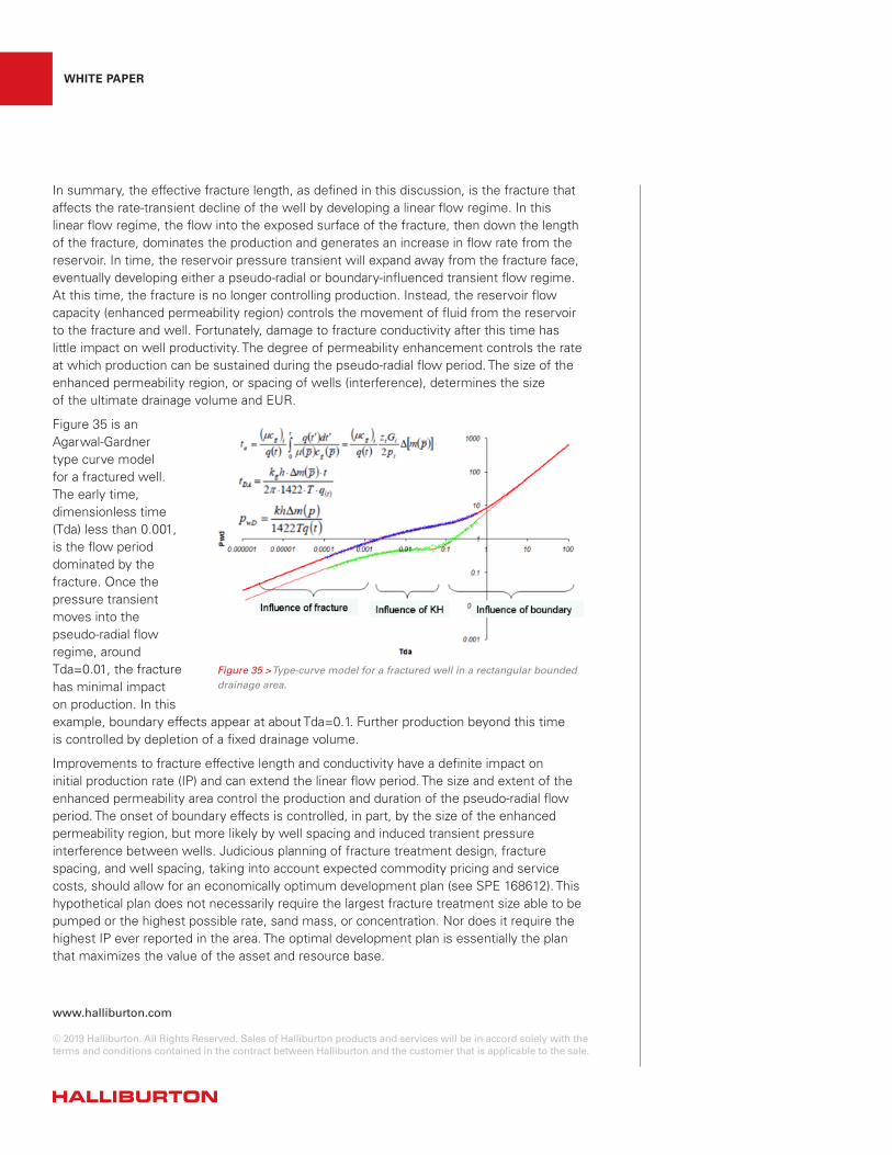
In summary, the effective fracture length, as defined in this discussion, is the fracture that affects the rate-transient decline of the well by developing a linear flow regime. In this linear flow regime, the flow into the exposed surface of the fracture, then down the length of the fracture, dominates the production and generates an increase in flow rate from the reservoir. In time, the reservoir pressure transient will expand away from the fracture face, eventually developing either a pseudo-radial or boundary-influenced transient flow regime. At this time, the fracture is no longer controlling production. Instead, the reservoir flow capacity (enhanced permeability region) controls the movement of fluid from the reservoir to the fracture and well. Fortunately, damage to fracture conductivity after this time has little impact on well productivity. The degree of permeability enhancement controls the rate at which production can be sustained during the pseudo-radial flow period. The size of the enhanced permeability region, or spacing of wells (interference), determines the size of the ultimate drainage volume and EUR.

Figure 35 is an Agarwal-Gardner type curve model for a fractured well. The early time, dimensionless time (Tda) less than 0.001, is the flow period dominated by the fracture. Once the pressure transient moves into the pseudo-radial flow regime, around Tda=0.01, the fracture has minimal impact on production. In this example, boundary effects appear at about Tda=0.1. Further production beyond this time is controlled by depletion of a fixed drainage volume.

Improvements to fracture effective length and conductivity have a definite impact on initial production rate (IP) and can extend the linear flow period. The size and extent of the enhanced permeability area control the production and duration of the pseudo-radial flow period. The onset of boundary effects is controlled, in part, by the size of the enhanced permeability region, but more likely by well spacing and induced transient pressure interference between wells. Judicious planning of fracture treatment design, fracture spacing, and well spacing, taking into account expected commodity pricing and service costs, should allow for an economically optimum development plan (see SPE 168612). This hypothetical plan does not necessarily require the largest fracture treatment size able to be pumped or the highest possible rate, sand mass, or concentration. Nor does it require the highest IP ever reported in the area. The optimal development plan is essentially the plan that maximizes the value of the asset and resource base.

Figure 35 > Type-curve model for a fractured well in a rectangular bounded drainage area.

WHITE PAPER

www.halliburton.com

© 2019 Halliburton. All Rights Reserved. Sales of Halliburton products and services will be in accord solely with the terms and conditions contained in the contract between Halliburton and the customer that is applicable to the sale.