what makes a replication successful?

Bachelor’s thesis

What makes a replication successful?An investigation of frequentist and Bayesian

criteria to assess replication success

Institut für Statistik

Ludwig-Maximilians-Universität München

Author Stephanie Armbruster

Supervisor Dr. Sabine Hoffmann

Place, time München, August 1, 2021

Abstract

Over the past decade, the scientific community has experienced the so called replication crisis. The repli-cation crisis follows from the discovery that many scientific studies lack replicability. This finding causedgreat havoc since non-replicability threatens the quality and validity of science in a philosophical as wellas practical sense. Replicability attributes a scientific study its fundamental purpose to gather evidence forthe designated research hypothesis. To ascertain the replicability of a certain study, replication studies areconducted. Despite the fundamental relevance and importance, the definitions for replication study andreplicability are controversially discussed. So far, no standard statistical method exists to evaluate whethera replication study either corroborates or falsifies its original study.

This thesis explores some of the controversies surrounding replicability, the reasons and concerns of thereplication crisis and its effects. It focuses on investigating popular frequentist, Bayesian and interval-based criteria to determine replication success. The criteria are assessed on three multi-lab examples and asimulation study with three different scenarios. They are influenced by distorting factors to varying degrees.The selected criteria differ in their meaningfulness as well as in their ability to detect distortions and handlevariation in treatment effect.

The complexity of replicability requires a wholesome approach. Therefore, the thesis recommends theusage of replication reports which incorporate a wider range of criteria to assess replication success. Itcloses by emphasizing the importance of a heightened awareness surrounding replicability and the increasedpopularity of proper statistical evaluation of replication studies in order to regain public trust in science andguarantee well founded scientific progress.

Contents

1 Introduction 6

2 Background 82.1 The replication crisis in science . . . . . . . . . . . . . . . . . . . . . . . . . . . . . . . . 8

2.1.1 Philosophy of Science and replication . . . . . . . . . . . . . . . . . . . . . . . . 82.1.2 Reasons for non-replicability of studies . . . . . . . . . . . . . . . . . . . . . . . 9

2.2 Replication studies . . . . . . . . . . . . . . . . . . . . . . . . . . . . . . . . . . . . . . 102.2.1 Definition of replicability and replication study . . . . . . . . . . . . . . . . . . . 102.2.2 Purpose of replication studies . . . . . . . . . . . . . . . . . . . . . . . . . . . . 112.2.3 Types of replication studies . . . . . . . . . . . . . . . . . . . . . . . . . . . . . 11

3 Methodology 133.1 Mathematical background . . . . . . . . . . . . . . . . . . . . . . . . . . . . . . . . . . 13

3.1.1 Notation . . . . . . . . . . . . . . . . . . . . . . . . . . . . . . . . . . . . . . . 133.1.2 Statistical fundamentals . . . . . . . . . . . . . . . . . . . . . . . . . . . . . . . 13

3.2 Overview of methods: definition, explanation and criticism . . . . . . . . . . . . . . . . . 183.2.1 Selection of frequentist and Bayesian criteria . . . . . . . . . . . . . . . . . . . . 183.2.2 Criteria and their assumptions . . . . . . . . . . . . . . . . . . . . . . . . . . . . 183.2.3 General remarks on meta-analysis . . . . . . . . . . . . . . . . . . . . . . . . . . 213.2.4 Methods for one replication . . . . . . . . . . . . . . . . . . . . . . . . . . . . . 213.2.5 Methods for multiple replications . . . . . . . . . . . . . . . . . . . . . . . . . . 37

3.3 Data sets - Multi-lab analysis . . . . . . . . . . . . . . . . . . . . . . . . . . . . . . . . . 403.3.1 Facial feedback hypothesis . . . . . . . . . . . . . . . . . . . . . . . . . . . . . . 413.3.2 Imagined contact hypothesis . . . . . . . . . . . . . . . . . . . . . . . . . . . . . 413.3.3 Sunk costs hypothesis . . . . . . . . . . . . . . . . . . . . . . . . . . . . . . . . 42

3.4 Simulation study . . . . . . . . . . . . . . . . . . . . . . . . . . . . . . . . . . . . . . . 433.4.1 Purpose . . . . . . . . . . . . . . . . . . . . . . . . . . . . . . . . . . . . . . . . 433.4.2 Methodological approach . . . . . . . . . . . . . . . . . . . . . . . . . . . . . . . 433.4.3 Generating the simulation study . . . . . . . . . . . . . . . . . . . . . . . . . . . 45

3.5 Application to multi-lab examples and simulation data . . . . . . . . . . . . . . . . . . . 463.5.1 Software and packages . . . . . . . . . . . . . . . . . . . . . . . . . . . . . . . . 463.5.2 Pre-processing of the multi-lab examples . . . . . . . . . . . . . . . . . . . . . . 473.5.3 Method implementation in R . . . . . . . . . . . . . . . . . . . . . . . . . . . . . 47

4 Results 504.1 Criteria for one replication . . . . . . . . . . . . . . . . . . . . . . . . . . . . . . . . . . 50

4.1.1 Facial feedback hypothesis . . . . . . . . . . . . . . . . . . . . . . . . . . . . . . 51

1

CONTENTS

4.1.2 Imagined contact hypothesis . . . . . . . . . . . . . . . . . . . . . . . . . . . . . 524.1.3 Sunk cost hypothesis . . . . . . . . . . . . . . . . . . . . . . . . . . . . . . . . . 534.1.4 Simulation study - scenario 1 . . . . . . . . . . . . . . . . . . . . . . . . . . . . . 544.1.5 Simulation study - scenario 2 . . . . . . . . . . . . . . . . . . . . . . . . . . . . . 554.1.6 Simulation study - scenario 3 . . . . . . . . . . . . . . . . . . . . . . . . . . . . . 56

4.2 Criteria for one replication on pooled data . . . . . . . . . . . . . . . . . . . . . . . . . . 564.2.1 Estimation of heterogeneity . . . . . . . . . . . . . . . . . . . . . . . . . . . . . 564.2.2 Implementation of replication success criteria . . . . . . . . . . . . . . . . . . . . 57

4.3 Criteria for multiple replications . . . . . . . . . . . . . . . . . . . . . . . . . . . . . . . 584.3.1 Facial feedback hypothesis . . . . . . . . . . . . . . . . . . . . . . . . . . . . . . 594.3.2 Imagined contact hypothesis . . . . . . . . . . . . . . . . . . . . . . . . . . . . . 594.3.3 Sunk cost hypothesis . . . . . . . . . . . . . . . . . . . . . . . . . . . . . . . . . 594.3.4 Simulation study - scenario 1 . . . . . . . . . . . . . . . . . . . . . . . . . . . . . 614.3.5 Simulation study - scenario 2 . . . . . . . . . . . . . . . . . . . . . . . . . . . . . 614.3.6 Simulation study - scenario 3 . . . . . . . . . . . . . . . . . . . . . . . . . . . . . 624.3.7 Graphical summary: non-central confidence interval . . . . . . . . . . . . . . . . 62

4.4 The influence of a one-sided prior distribution . . . . . . . . . . . . . . . . . . . . . . . . 644.4.1 One-sided priors for Bayes factors . . . . . . . . . . . . . . . . . . . . . . . . . . 644.4.2 One-sided priors for posterior equal-tailed credibility interval . . . . . . . . . . . 65

4.5 Assessment of assumptions . . . . . . . . . . . . . . . . . . . . . . . . . . . . . . . . . . 684.5.1 Assumption of normality . . . . . . . . . . . . . . . . . . . . . . . . . . . . . . . 684.5.2 Assumption of equal variance . . . . . . . . . . . . . . . . . . . . . . . . . . . . 69

5 Discussion 715.1 Discussion of criteria for one and multiple replications . . . . . . . . . . . . . . . . . . . 71

5.1.1 Criticism on frequentist criteria . . . . . . . . . . . . . . . . . . . . . . . . . . . 715.1.2 Criticism on Bayesian criteria . . . . . . . . . . . . . . . . . . . . . . . . . . . . 725.1.3 Criticism on interval-based methods . . . . . . . . . . . . . . . . . . . . . . . . . 735.1.4 Criticism on small telescope . . . . . . . . . . . . . . . . . . . . . . . . . . . . . 745.1.5 Criticism on sceptical p-value . . . . . . . . . . . . . . . . . . . . . . . . . . . . 74

5.2 The power of the Bayesian factor and snapshot hybrid . . . . . . . . . . . . . . . . . . . . 745.3 The strength of confidence and credibility intervals . . . . . . . . . . . . . . . . . . . . . 775.4 Success or failure - criticism of a binary classification . . . . . . . . . . . . . . . . . . . . 775.5 Limitations and further investigation . . . . . . . . . . . . . . . . . . . . . . . . . . . . . 78

6 Conclusion 796.1 Suggestions and alternatives for the statistical evaluation of replication success . . . . . . 79

6.1.1 Replication report . . . . . . . . . . . . . . . . . . . . . . . . . . . . . . . . . . . 796.1.2 Alternative approaches . . . . . . . . . . . . . . . . . . . . . . . . . . . . . . . . 806.1.3 Essential role of preregistration and disclosure . . . . . . . . . . . . . . . . . . . 80

6.2 Current situation and outlook . . . . . . . . . . . . . . . . . . . . . . . . . . . . . . . . . 816.2.1 Concerns regarding replicability . . . . . . . . . . . . . . . . . . . . . . . . . . . 816.2.2 Consequences of the replication crisis - in public and science . . . . . . . . . . . . 826.2.3 The battle against the myth of science . . . . . . . . . . . . . . . . . . . . . . . . 83

A Mathematical and statistical foundations 85A.1 Fundamental empirical estimators . . . . . . . . . . . . . . . . . . . . . . . . . . . . . . 85A.2 Cochran’s Q test . . . . . . . . . . . . . . . . . . . . . . . . . . . . . . . . . . . . . . . . 86

2

CONTENTS

A.3 Correlation . . . . . . . . . . . . . . . . . . . . . . . . . . . . . . . . . . . . . . . . . . 86A.4 Fisher transformation . . . . . . . . . . . . . . . . . . . . . . . . . . . . . . . . . . . . . 87A.5 Bayes Theorem . . . . . . . . . . . . . . . . . . . . . . . . . . . . . . . . . . . . . . . . 88

B Descriptive analysis of multi-lab examples 89B.1 Facial feedback . . . . . . . . . . . . . . . . . . . . . . . . . . . . . . . . . . . . . . . . 89B.2 Imagined contact hypothesis . . . . . . . . . . . . . . . . . . . . . . . . . . . . . . . . . 90B.3 Sunk cost hypothesis . . . . . . . . . . . . . . . . . . . . . . . . . . . . . . . . . . . . . 90

C Overview of criteria results 92

D Credibility intervals 96

3

List of Figures

4.1 90% credibility interval for the one-sided posterior distribution . . . . . . . . . . . . . . . 594.2 Overview: mean difference between condition and control group and Cohen’s d - facial

feedback hypothesis . . . . . . . . . . . . . . . . . . . . . . . . . . . . . . . . . . . . . . 604.3 Overview: mean difference between condition and control group and Cohen’s d - imagined

contact hypothesis . . . . . . . . . . . . . . . . . . . . . . . . . . . . . . . . . . . . . . . 604.4 Overview: mean difference between condition and control group and Cohen’s d - sunk cost

hypothesis . . . . . . . . . . . . . . . . . . . . . . . . . . . . . . . . . . . . . . . . . . . 614.5 Overview: mean difference between condition and control group and Cohen’s d - scenario 1 624.6 Overview: mean difference between condition and control group and Cohen’s d - scenario 2 634.7 Overview: mean difference between condition and control group and Cohen’s d - scenario 3 634.8 Non-central confidence intervals for Cohen’s d - multi-lab examples and simulation data . 644.9 Posterior equal-tailed credibility interval with one- and two-sided JZS prior . . . . . . . . 674.10 QQ-Plot for multi-lab hypotheses . . . . . . . . . . . . . . . . . . . . . . . . . . . . . . . 694.11 Density plot for multi-lab hypotheses . . . . . . . . . . . . . . . . . . . . . . . . . . . . . 704.12 Difference ∆ in variance between condition and control group for multi-lab hypotheses . . 70

5.1 Correlation coefficients for all datasets and default effect sizes for snapshot hybrid . . . . . 76

D.1 Credibility interval for facial feedback hypothesis . . . . . . . . . . . . . . . . . . . . . . 97D.2 Credibility interval for imagined contact hypothesis . . . . . . . . . . . . . . . . . . . . . 98D.3 Credibility interval for sunk costs hypothesis . . . . . . . . . . . . . . . . . . . . . . . . . 99D.4 Credibility interval for simulation data in scenario 1 . . . . . . . . . . . . . . . . . . . . . 100D.5 Credibility interval for simulation data in scenario 2 . . . . . . . . . . . . . . . . . . . . . 101D.6 Credibility interval for simulation data in scenario 3 . . . . . . . . . . . . . . . . . . . . . 102D.7 Density of θ and τ2 for facial feedback hypothesis . . . . . . . . . . . . . . . . . . . . . . 103D.8 Density of θ and τ2 for sunk costs hypothesis . . . . . . . . . . . . . . . . . . . . . . . . 103D.9 Density of θ and τ2 for imagined contact hypothesis . . . . . . . . . . . . . . . . . . . . . 104D.10 Density of θ and τ2 for scenario 1 . . . . . . . . . . . . . . . . . . . . . . . . . . . . . . 104D.11 Density of θ and τ2 for scenario 2 . . . . . . . . . . . . . . . . . . . . . . . . . . . . . . 105D.12 Density of θ and τ2 for scenario 3 . . . . . . . . . . . . . . . . . . . . . . . . . . . . . . 105

4

List of Tables

3.1 Results for facial feedback hypothesis in the original paper . . . . . . . . . . . . . . . . . 413.2 Results for imagined contact hypothesis in original paper . . . . . . . . . . . . . . . . . . 423.3 Results for sunk cost hypothesis in original paper . . . . . . . . . . . . . . . . . . . . . . 42

4.1 Results for facial feedback hypothesis . . . . . . . . . . . . . . . . . . . . . . . . . . . . 524.2 Results for imagined contact hypothesis . . . . . . . . . . . . . . . . . . . . . . . . . . . 534.3 Results for sunk cost hypothesis . . . . . . . . . . . . . . . . . . . . . . . . . . . . . . . 544.4 Results for simulation scenario 1 . . . . . . . . . . . . . . . . . . . . . . . . . . . . . . . 554.5 Results for simulation scenario 2 . . . . . . . . . . . . . . . . . . . . . . . . . . . . . . . 564.6 Results for simulation scenario 3 . . . . . . . . . . . . . . . . . . . . . . . . . . . . . . . 574.7 EB estimates of effect size heterogeneity . . . . . . . . . . . . . . . . . . . . . . . . . . . 574.8 Results overview for replication success criteria applied to pooled multi-lab examples . . . 584.9 Results for facial feedback hypothesis . . . . . . . . . . . . . . . . . . . . . . . . . . . . 594.10 Results for imagined contact hypothesis . . . . . . . . . . . . . . . . . . . . . . . . . . . 594.11 Results for sunk cost hypothesis . . . . . . . . . . . . . . . . . . . . . . . . . . . . . . . 614.12 Results for simulation scenario 1 . . . . . . . . . . . . . . . . . . . . . . . . . . . . . . . 614.13 Results for simulation scenario 2 . . . . . . . . . . . . . . . . . . . . . . . . . . . . . . . 624.14 Results for simulation scenario 3 . . . . . . . . . . . . . . . . . . . . . . . . . . . . . . . 624.15 Bayes factor comparison for facial feedback hypothesis . . . . . . . . . . . . . . . . . . . 654.16 Bayes factor comparison for imagined contact hypothesis . . . . . . . . . . . . . . . . . . 654.17 Bayes factor comparison for sunk cost hypothesis . . . . . . . . . . . . . . . . . . . . . . 654.18 Bayes factor comparison for scenario 1 . . . . . . . . . . . . . . . . . . . . . . . . . . . . 664.19 Bayes factor comparison for scenario 2 . . . . . . . . . . . . . . . . . . . . . . . . . . . . 664.20 Bayes factor comparison for scenario 3 . . . . . . . . . . . . . . . . . . . . . . . . . . . . 664.21 Shapiro-Wilks test results . . . . . . . . . . . . . . . . . . . . . . . . . . . . . . . . . . . 68

B.1 Replication studies for facial feedback hypothesis . . . . . . . . . . . . . . . . . . . . . . 89B.2 Replication studies for imagined contact hypothesis . . . . . . . . . . . . . . . . . . . . . 90B.3 Replication studies for sunk cost hypothesis . . . . . . . . . . . . . . . . . . . . . . . . . 91

C.1 Overview over criteria to define replication success: facial feedback hypothesis . . . . . . 93C.2 Overview over criteria to define replication success: imagined contact hypothesis . . . . . 94C.3 Overview over criteria to define replication success: sunk cost hypothesis . . . . . . . . . 95

5

Chapter 1

Introduction

Over the past decade, the scientific community has faced a fundamental crisis - the replication crisis. Thecrisis was triggered when the first sentence in Ioannidis, 2005 read: “It can be proven that most claimedresearch findings are false.” (p. 696)From then onward, the awareness of the fundamental importance of replicability and the rate of activeimplementation of replication studies have steadily increased (e.g. Pashler and Wagenmakers, 2012, Zwaanet al., 2018). Nevertheless, a lack of replicability continues to loom over Psychology as much as SocialScience, Economics and Cancer biology (Pashler and Wagenmakers, 2012). It therefore remains a problemaffecting science as a whole.

But what exactly does the replication crisis entail and replicability mean? And why all the excitementaround it?

The replication crisis describes a deep and troublesome dilemma in which the scientific community findsitself - many scientific studies praised as advancement of science cannot be reconstructed in their findings.As a consequence to non-replicability, their validity is highly questionable (Nelson et al., 2018). Replicabil-ity - meaning the ability to obtain similar results from a different sample analyzed with the same methods -is a cornerstone of science (Zwaan et al., 2018). Without it, a study cannot serve as adequate proof to a sci-entific hypothesis and is thus rendered useless (Dunlap, 1926). This explains the gravity of the replicationcrisis - it calls the quality and validity of science into question (German Research Foundation, 2017).

Performing replication studies has been widely adopted as an effective remedy for a loss of trust in scientificfindings (e.g. Open Science Collaboration, 2015, Hunter, 2001). It implies that studies are repeatablyconducted - oftentimes by other research group - as similar to the original set-up as possible and analyzedaccording to the same methods.

If we accept the importance and relevance of replication studies for scientific discovery, we remain with thepractical question of determining whether a replication study is successful or unsuccessful? How can weascertain whether a replication study corroborates or falsifies the effect size estimated in the original study?

There is a broad spectrum of methods available on how to define replication success, ranging from simplefrequentist p-value calculations (e.g. Klein et al., 2014) to complex Bayesian hierarchical models (e.g.Marsman et al., 2017).

This thesis strives to give a short introduction into the replication crisis, its reasons, relevance and conse-quences. It continues to identify and explain the most promising and popular criteria to determine replica-

6

tion success. It focuses on investigating the performance of the selected criteria based on multi-lab exam-ples and simulation data with a special focus on possible distortions through publication bias and selectivereporting. It concludes with some additional remarks on measures taken to increase replicability and oncultural challenges to overcome the replication crisis as well as concerns surrounding replication studies.

7

Chapter 2

Background

2.1 The replication crisis in science

Ioannidis, 2018 recounts the anecdote that in the early years of the Royal Society, researchers declaring tohave made a scientific discovery would repeat the experiment in the presence of their colleagues to provetheir claim. They basically conducted a replication study. More recently, in 1998, the FDA introduced thetwo trial rule which requires a minimum of two independent trials with a positive outcome for the registra-tion of a new treatment. Hence they actively test for the replicability of significant findings (Rosenkranz,2021).

Obviously, the awareness around the importance of replication and replicability is not an invention of currenttimes (Nosek and Lakens, 2014). However, those early precautions taken to guarantee replicability werethe exception, not the rule. In general, over the course of time, the notion of external accountability forscientific findings has increasingly vanished - only to be re-established as a consequence to the replicationcrisis now (e.g. Zwaan et al., 2018).

The long lasting neglect of replication studies and the necessity of explicit checks for replicability arepuzzling since it is self explanatory that scientific claims can only gain credibility if they can be replicatedand result in similar effect estimates for each replication study (Nosek and Errington, 2017).

2.1.1 Philosophy of Science and replication

From a more philosophical perspective, it can be argued that only replicability turns scientific findings intoproper evidence.

Karl Popper created a Demarcation Criterion between Science and Non-Science (Musgrave and Pigden,2021, Zwaan et al., 2018, S. Schmidt, 2009). According to this criterion, science is defined by the ability toempirically falsify its claims. This indicates that empirical observations must have the potential to prove ascientific hypothesis wrong. Replicability - the ability to replicate - is an essential property for any scientificstudy since it is a core method for scientific falsification (S. Schmidt, 2009). In keeping with statements byPopper and Dunlap, Zwaan et al., 2018 declares that “a finding needs to be repeatable to count as scientificdiscovery”. (p. 2)

Ideally, as a hypothesis cycles through multiple rounds of replications, it becomes either more robust andrefined or looses credibility and vanishes (Zwaan et al., 2018). According to the theory of sophisticated fal-sificationism, this iterated verification process is called a research program. It can be either progressive - in

8

2.1. THE REPLICATION CRISIS IN SCIENCE

case of repeated affirmation - or degenerative - in case of repeated refutation (Zwaan et al., 2018, Musgraveand Pigden, 2021).A progressive research program serves as proof of existing replicability. After having withstood severalrefutation attempts under the condition of being potentially refutable, a theory and its experiment aredeemed good science and probably true (Musgrave and Pigden, 2021).

Failure to reproduce does not necessarily mean the entire theory behind the hypothesis is false. We ratherhave to test for additional essential characteristics to the study which might have been neglected in the repli-cation study but were present in the original study. Hence, with every iteration, the degenerative researchprogram becomes more specific until it reaches a certain threshold of irrelevance (Musgrave and Pigden,2021). A degenerative research program that remains degenerative throughout the iterative testing servesas (indirect) falsification of the underlying hypothesis (Zwaan et al., 2018). Alternatively, a degenerativeresearch program might become progressive if through further specification, studies become replicable.Consequently, replications studies contributed to developing a theory in more detail (Nosek and Lakens,2014).

2.1.2 Reasons for non-replicability of studies

The replication crisis does not root in one cause but stems from a broad range of problematic yet establishedpractices and complex interaction between them. Next to outright fraud, questionable research practices,methodological flexibility and the procedure of scientific publication contribute to a serious lack of replica-bility (Laraway et al., 2019).

Researcher’s degree of freedom and methodological flexibility demonstrate a high distorting potential (Fer-guson and Heene, 2012, Hoffmann et al., 2020). Researchers can choose analysis techniques and statisticalmodels freely to best account for the study data and come to the desired conclusion. All distorting fac-tors play their part in establishing overconfidence in an effect as well as in overestimating the effect size(Hoffmann et al., 2020).

Three major contributors to non-replicability and symptoms of methodological flexibility are publicationbias, P-hacking and HARKing.

While some distorting factors have been addressed, others have remained until today (Nosek and Lakens,2014). Overcoming the replication crisis is still very much an ongoing mission.

Publication bias

Publication bias describes a phenomenon with many nuances and a long history. Rosenthal, 1979 alreadyidentified its risks and invented a name for it - the file drawer problem. Zwaan et al., 2018 defines publicationbias as “the process by which research findings are selected based on the extent to which they providesupport for a hypothesis” (p. 2). Publication bias implies that studies with proof of a significant effectare published with higher probability than those with a non-significant effect - the latter are relegated intothe researcher’s drawer. This also extends to novel research findings as well. New results are regarded asmore worthy of publishing than replicated and already explored results (Ioannidis, 2018, Nosek and Lakens,2014).

As a direct consequence, published studies do not correctly represent all conducted studies but are a sampleskewed toward successful studies with significant and / or new effects (F. Schmidt and Oh, 2016). Publica-tion bias automatically leads to a greater rate of false positive effect estimates than expected.Locating the fault solely with the publishing companies and their publishing policies, however, is not cor-

9

2.2. REPLICATION STUDIES

rect. Publication bias can be as much internally as externally motivated. Researchers refrain from submit-ting non-significant findings either because they are convinced of the unpublishable quality of their resultsor due to loyalty to a certain hypothesis, discredited by the study (Ferguson and Heene, 2012, Zwaan et al.,2018, Rosenthal, 1979).

P-hacking

P-hacking is also known under multiple alternative names, such as fishing for significance or researcherdegrees of freedom. According to Zwaan et al., 2018, it describes a scientific practice in which researchersperform as many statistical tests as necessary until they achieve a significant effect. While with everytest the likelihood of finding a significant effect increases, the power and replicability of such test steadilydecrease. P-hacking is usually no intentional choice but a result of ignorance paired with confirmation bias.The researcher is led to believe the test resulting in a significant effect was the best and most appropriatefrom the beginning (Zwaan et al., 2018, Nelson et al., 2018). According to Nelson et al., 2018, P-hackingposes “the biggest threat to the integrity” of science (p. 517).

It is deeply linked to publication bias - significant results mean likely publication, mean higher record ofpapers and thus greater scientific reputation.

Closely related to P-hacking is fishing for the most surprising effect. It denotes the phenomenon in whichthe effect size calculated based on the original sample is notably greater than the effect size estimated bythe replication studies due to actively constructing a surprisingly big and conclusive effect (Nelson et al.,2018).

HARKing

HARKing describes researchers formulating or changing their hypotheses post-hoc after seeing the data.The term and concept were first introduced by Kerr, 1998. HARKing is short for Hypothesizing after theresults are known. It stands in stark contrast to the usual (and desirable) hypothetico-deductive approach.The latter characterizes a process in which researchers determine their research hypothesis based on somea priori knowledge and subsequently design an experiment to test their hypothesis. The potential scientificmeaning of a certain study is defined before the data collection. HARKing inverts this process. Researchersperform HARKing when they phrase their hypothesis a posteriori after having detected certain patterns inthe data. However, they still pretend to have determined it a priori (Kerr, 1998).

HARKing comes in different versions and can be deemed a consequence of publication bias. If a researcheradapts the hypothesis based on the data, the data will by definition lead to a significant effect and thus bemore likely to be published. A simple remedy for HARKing are replication studies. They assess if oneis “HARKing to explain an illusion” (Kerr, 1998, p. 207) or if the effect actually exists in reality, i.e. isreplicable. For more detailed insight into the phenomenon of HARKing and reasons why HARKing is sucha wide spread research practice, the reader might refer to Kerr, 1998.

2.2 Replication studies

2.2.1 Definition of replicability and replication study

We have ascertained that while replicability is a central features to science it is non-existent in many studiesfor multiple reasons. But what exactly defines replicability? When can we justifiably term a study asa replication study? So far, we have not encountered a formal definition. Deploying one is challengingbecause replicability “is a confused terminology” (Plesser, 2018, p. 1).

10


Reproducibility vs. replicability

The first step in clarifying the definition of replicability and replication studies is distinguishing betweenreproducibility and replicability.

Reproducibility describes a preliminary stage to replicability. If a study is reproducible, the original exper-iment in itself is conclusive and correctly performed, e.g. rerunning the code generates the same outcomeas given in the original paper (Plesser, 2018). Reproducibility is determined based on the original data.Replicability relies on new data gathered according to the set-up of the original study.

Despite or maybe because of its relevance, replication or replicability are described by a myriad of differentdefinitions. Gundersen, 2021 for example includes 16 potential understandings of replicability.

For the purpose of this thesis, we limit ourselves to two terms and respective explanations.

1. replication (study): both process and outcome of repeating a study, i.e. to draw a new sample accord-ing to the original settings

2. replicability: the ability to perform a successful replication, i.e. from new data collected in a replica-tion study obtain a result matching the original output (Goodman et al., 2016)

2.2.2 Purpose of replication studies

The purpose of a replication study is to assess the replicability of a study and its inherent truth. “[I]f a findingcan be reliably repeated, it is likely to be true, and if it cannot be, its truth is in question.” (Goodman et al.,2016, p. 4) In some sense, replicability therefore allows a mathematical capturing of reality (Goodmanet al., 2016).

Thus, the goal is a sort of binary classification. We classify a replication study as a success or a failure anddetermine whether it corroborates or falsifies the original study.

However, the question remains - what does success in replication actually imply? According to Bayarriand Mayoral, 2002, a replication is successful when it achieves the goals it was designated for. The goalsoriginate from a wide range of possibilities with the most popular ones including,

- Reduction of error: exact replications are conducted to gather more data and decrease the randomerror in estimates.

- Validation of findings: independent direct replications validate the original findings by leading tosimilar conclusions (frequently non-zero effect size).

- Extension of conclusions: conceptual replications assess how changes in experimental set-up influ-ence the experimental output and to which extent the original hypothesis can be generalized (fre-quently on different sub-populations).

- Bias detection: replication studies which are conducted so they are not influenced by any distort-ing factors assess whether the original findings were likely subjected to any distorting factors (e.g.publication bias).

2.2.3 Types of replication studies

In order to fulfill the various demands placed on replication studies, there are multiple different types ofreplication studies which vary in design and analysis.

11


Direct replications

The understanding of replication in this thesis corresponds to the definition of a direct replication in theliterature (Nosek and Errington, 2017). A direct replication can be understood as a study in which allrelevant settings of the original study are recreated. Relevant means essential in order to capture the sameinformation in the replication study as it has been in the original study (Zwaan et al., 2018, Nosek andErrington, 2017, Open Science Collaboration, 2015, Klein et al., 2014).

Given that studies are experimental in their nature, determining which features are essential or irrelevantfor the effect proves to be a challenge. The big difficulty is to distinguish whether the reason for non-replicability can be found in the effect itself rather than in a change of experimental setting which left outan unknown but apparently relevant feature to reproduce the original study (Zwaan et al., 2018)? Thisquestion captures the main argument leveraged to dismiss the suitability of direct replications to assessreplicability (Stroebe and Strack, 2014).

Simons, 2014 argues that the distinction of relevant and irrelevant experimental conditions comes in ac-cordance with a certain degree of generalization of scientific findings and its underlying theory. Deferringdifferences between original and replication study solely to hidden mediators renders a theory simulta-neously unfalsifiable and unprovable. “Direct replication is the only way to make sure our theories areaccounting for signal and not noise.” (Simons, 2014, p. 79)

Notwithstanding, replicability in the sense of successful direct replications, whatever its exact definition,cannot be equated with validity (Nosek and Errington, 2017, German Research Foundation, 2017). It merelyincreases the probability that a certain hypothesis is true based on one specific methodology.

Conceptual replications

In order to verify the existence without methodological condition, the hypothesis requires further verifi-cation independent of the statistical approach. This is achieved by conducting the higher acknowledgedversion of replication studies - conceptual replications. The primary goal of conceptual replication is todeepen theoretical understanding. It specifies the research theory, but rarely inquires whether the theory inits fundamental outline is actually correct (Nosek and Lakens, 2014).

Conceptual replications test a hypothesis with different methods to prove that the underlying theory iscorrect - and the effect does not happen to be an artefact from applying a certain statistical approach tothe data (Nosek and Errington, 2017). This allows the conceptual replication to deliver evidence for an“extension of the theory to a new context” (Zwaan et al., 2018 p. 4).

In combination, direct and conceptual replication serve two purposes: it provides evidence for the repli-cability of an original finding and verifies the explanation of such finding (Nosek and Errington, 2017,Goodman et al., 2016).

The scientific community has not yet agreed upon one default method on how to determine success inreplication studies (e.g. Schweinsberg et al., 2016, Gundersen, 2021). This of course leaves great room forheated debate and scientific controversy (Goodman et al., 2016). The currently applied calculation criteriarange from simple p-value comparisons (e.g. Schweinsberg et al., 2016, Open Science Collaboration, 2015)to complex Bayesian random effect meta-analysis and Bayes factor calculations (e.g. Marsman et al., 2017,Ly et al., 2019, Verhagen and Wagenmakers, 2014).

In the framework of this thesis, successful replication means that the significant effect measured in theoriginal study corresponds to reality and is not a false-positive or overestimated effect due to distortingfactors such as publication bias, p-hacking or HARKing.

12

Chapter 3

Methodology

3.1 Mathematical background

3.1.1 Notation

Throughout the thesis, the theory behind the different criteria is presented in a consistent notation. Arbitraryparameters of interest are denoted by γ. θ stands for the raw mean difference. Its empirical estimate is writ-ten as θ. The standardized mean difference, also called Cohen’s d, is indicated by δ and the correspondingempirical estimate by d. µ traditionally stands for the mean of a variable and is empirically estimated by x.

σ2 represents the variation within each sample, while τ2 stands for the heterogeneity or variation in treat-ment effect between studies. The empirical estimates are denoted by s2 and τ2 respectively.

For the sake of completeness, we provide the empirical estimators in appendix A.

3.1.2 Statistical fundamentals

While the most central or less known statistical concepts are explained in this section, more popular methodsare elaborated in appendix A.

One-sided t-test

In the context of the replication crisis, the primary interest lies in testing a one-sided hypothesis. The one-sided t-test is a basic statistical test used to determine if a parameter is smaller or greater than a certain valueµ0 (Fahrmeir et al., 2016).

Hence, the hypothesis can be expressed asVersion 1:

H0 : µ ≤ µ0 (3.1)

H1 : µ > µ0 (3.2)

or alternatively,

13

3.1. MATHEMATICAL BACKGROUND

Version 2:

H0 : µ ≥ µ0 (3.3)

H1 : µ < µ0 (3.4)

The main conditions for using a one-sided t-test are:

1. The data points xi originate from a normal distribution N(µ, σ2).

2. The data points xi are sampled independently of each other (iid).

If these conditions are fulfilled the t-test is an exact test.

The test is applicable for situations in which mean µ and variance σ2 are unknown and therefore have to beestimated by the empirical mean x and variance s2.

The t-test is calculated as

t =√nx− µ√s2

(3.5)

Under the null hypothesis H0 the test statistic t is distributed according to the t-distribution with n − 1

degrees of freedom.

tH0∼ t(n− 1)

Inserting data into formula 3.5 leads to t0.The p-value is determined depending on the null hypothesis.Version 1:

p = P (t ≥ t0|H0) = 1− T (t0) (3.6)

Version 2:

p = P (t ≤ t0|H0) = T (t0) (3.7)

where T is the cumulative t-distribution function. It can be approximated by Φ, the cumulative normaldistribution function, if the sample size n is greater or equal to 30.The effect is significant on a significance level of α if p ≤ α. The most common choice for α is 0.05

(Fahrmeir et al., 2016).

Apart from the degrees of freedom, the t-statistic has another parameter which characterizes its appearance- the non-centrality parameter c (Smithson, 2003, Bayarri and Mayoral, 2002). It has the form

c =µ− µ0

σ√n

= δ√n (3.8)

with µ the actual expectation of the observed variable and µ0 the assumed expectation under the null hy-pothesis.It is easy to see why the non-centrality is neglected during classical hypothesis testing. If the null hypoth-esis holds, the non-centrality parameter c is equal to zero and the t-distribution becomes central. If thenull hypothesis, however, does not hold, the non-centrality parameter has to be acknowledged in order to

14


construct an accurate confidence interval (Smithson, 2003). This applies in chapter 3.2.5 when non-centralconfidence intervals of the effect size are used to determine replication success.

The application of a t-test can be expanded from one sample to two samples, resulting in the two-groupt-test with null hypothesis H0 : θ ≤ 0 or H0 : θ ≥ 0.θ denotes the difference between the expected values of the two groups under the null hypothesis, θ =

µ1 − µ2.

The conditions for the one sample t-test have to be equally fulfilled in the two sample case. Additionally,we assume that the two samples are independent of each other and have the same variance σ2

1 = σ22 . The

formula for the two-group t-test starkly resembles formula 3.5

t =(x1 − x2)− θ√s2p ·√

1n1

+ 1n2

(3.9)

where s2p is the pooled variance.

Under the null hypothesis t is distributed according to a central t-distribution with n1 + n2 − 2 degrees offreedom, t H0∼ t(n1 + n2 − 2) (Kelley et al., 2007).

Validity of normality assumption for big sample sizes

We can assume that - given a sufficiently large sample size - the mean x is normally distributed and inde-pendent of the distribution of the individual observations xi due to the central limit theorem. Consequently,the t-test for one and two samples can be applied as an approximate test even if the random variable doesnot fulfill the normal distribution condition (Fahrmeir et al., 2016, Ghasemi and Zahediasl, 2012).

Cohen’s d

Cohen’s d is a popular method to measure effect size. It calculates the population standardized meandifference between two groups with expected value µ1 and µ2 respectively and standard deviation σ for thepopulation (Kenny and Judd, 2019 Cohen, 2013).

δ =µ1 − µ1

σ=θ

σ(3.10)

Cohen’s d is approximated by standardizing the empirical mean difference between two groups with theempirical estimate of the pooled standard deviation, sp , (Welkowitz et al., 2006)

d =x1 − x2

sp=

θ

sp(3.11)

The main benefit of Cohen’s d is comparability across studies since it is scaled. This is especially relevantfor meta-analysis in which studies can be summarized despite having measured the same dependent variableon different scales (Diener, 2010).

The effect sizes within this thesis are frequently calculated as Cohen’s d. Some hypotheses in chapter 3.2are formulated based on δ, while others are based on the raw mean difference between condition and controlgroup, denoted by θ. Due to the direct relationship between both effect measures, the hypotheses can beeasily converted.

15


Bayes factor

The Bayes factor serves as a primary Bayesian tool in statistical inference and as a main alternative tofrequentist hypothesis testing (Ly et al., 2019). Several methods presented in chapter 3.2 utilize the Bayesfactor to determine replication success.

The Bayes factor calculates the factor by which the data is more likely to have been drawn from the nullhypothesis than from the alternative hypothesis while including prior knowledge and expertise (Goodman,1999, Scheibehenne et al., 2016).

The null and alternative hypothesis are defined as

H0 : γ ∈ Θ0 (3.12)

H1 : γ ∈ Θ1 (3.13)

where Θ0 and Θ1 are some disjunct partitions of R.For the Bayesian criteria concerned with establishing the existence or non-existence of an effect in thisthesis, we set Θ0 = 0.

As aforementioned, the basic idea behind the Bayes factor is to decide for the hypothesis for which thecollected data speaks the most (Marsman et al., 2017). This notion is mathematically expressed by theposterior odds of the probability for each hypothesis conditional on the data x.The Bayes factor BF01 denotes the factor by which the prior odds, oddspriori = P (H0)

P (H1) , is updated toobtain the posterior odds (Bolstad and Curran, 2016)

oddspost =P (H0|x)

P (H1|x)= oddspriori ·BF01 (3.14)

with

BF01 =f (x|H0)

f (x|H1)(3.15)

In case no prior probability of either hypothesis exists, one might choose to assume the null and alternativehypothesis to be equally likely. Mathematically, this means selecting an uninformative prior distribution,a Bernoulli distribution with p = 1

2 . This leads to P (H0) = P (H1) = 12 and P (H0)

P (H1) = 1 (Rouder et al.,2009, van Ravenzwaaij and Etz, 2021).This a-priori choice is rather common and regarded as objective (Berger and Delampady, 1987). It allows asimplification of the formula 3.14 to

P (H0|x)

P (H1|x)=f (x|H0)

f (x|H1)(3.16)

Consequently, we can justify drawing conclusion regarding the posterior odds based on the Bayes factor(Ly et al., 2019).

The Bayes factor is calculated as an average likelihood ratio. The likelihood is determined by the densityfunction f of X and the prior density p1 and p2 for parameter γ depending on the hypothesis (Kauermann

16


and Hothorn, 2020, Verhagen and Wagenmakers, 2014, Morey and Rouder, 2011)

BF01 =f (x|Θ0)

f (x|H1)=

∫γ∈Θ0

f (x|γ) p1(γ) dγ∫γ∈Θ1

f (x|γ) p2(γ) dγ(3.17)

f (x|Θ0) and f (x|Θ1) are called marginal likelihood (Verhagen and Wagenmakers, 2014, Ly et al., 2019,Morey and Rouder, 2011). The null and alternative hypothesis differ in their subjective belief in the param-eter γ - and are consequently assigned different prior distributions, p1 and p2.

When the null hypothesis entails a point estimate γ0, the entire probability mass of the prior distribution isconcentrated on γ0 (Wagenmakers, Verhagen, et al., 2016)

p1(γ) =

1 if γ = γ0

0 else(3.18)

This kind of distributions is called a one-point density.

The alternative hypothesis could e.g. suspect positive values for γ, resulting in some one-sided prior distri-bution with its probability mass scattered across a range of positive values.

The interpretation of the Bayes factor is rather intuitive. The data x is by the factor BF01 more likely orunlikely, depending on BF01 > 1 (likely) or BF01 < 1 (unlikely), to have been gathered under assumptionH0 than H1 (Rouder et al., 2009, Verhagen and Wagenmakers, 2014, Scheibehenne et al., 2016, Ly et al.,2019).

The relationship can easily be inverted by

BF10 =f (x|Θ1)

f (x|Θ0)=

1

BF01(3.19)

BF10 subsequently tells us by which factor the data is more likely or unlikely to stem from the alternativehypothesis compared to the null hypothesis.

Advantages of the Bayes factor

The Bayes factor has advantages over the ordinary t-test because it

- allows accepting the null hypothesis, compared to only being able to not reject it in standard nullhypothesis significance testing (Verhagen and Wagenmakers, 2014).

- is a more precise and realistic measurement of certainty, compared to p-values which tend to overstatethe evidence against the null hypothesis (Rouder et al., 2009).

Its interpretation is also “straightforward and natural” (Rouder et al., 2009, p. 228). Ly et al., 2019 addthat the Bayes factor allows considering evidence in sub stages while the data is still in the process ofcollection. The Bayes factor also incorporates Ockham’s razor, i.e. it accounts for the model complexityadditional to its predictive performance. This results since the prior probability mass is distributed across abigger parameter space for complex assumptions than it is for simpler ones, resulting in lower densities atindividual values including the true parameter value (Wagenmakers et al., 2010).

Classification of the Bayes factor

Jeffreys, 1961 suggests a classification of the Bayes factor according to its amount of evidence for the nullhypothesis according to its magnitude.

17

3.2. OVERVIEW OF METHODS: DEFINITION, EXPLANATION AND CRITICISM

BF01 > 3: some evidence for H0

BF01 > 10: strong evidence for H0

BF01 > 30: very strong evidence for H0

Jeffreys, 1961 also proposes redeeming BF01 as insufficient evidence if BF01 ∈ [ 13 , 3].

Hoijtink et al., 2016 criticize this general classification approach given that the probability of the boundaryvalues differ across different observed empirical estimates of the target variable. They propose a morecustomized approach to classifying the strength of evidence.

In this thesis, however, we hold on to the more generic classification of Bayes factor values.

Intervals as null hypothesis

“It is rare, and perhaps impossible, to have a null hypothesis that can be exactly modeled as γ = γ0”(Berger and Delampady, 1987, p. 320). When interested in effect sizes, a null effect is rarely realistic andfrequently too restrictive (Bayarri and Mayoral, 2002). Effects can either be influenced by random error orexhibit a non-zero effect size which is minuscule and irrelevant. Consequently, a null hypothesis should notbe limited to a zero point estimate but incorporate a zero-centered interval with a small ε

H0 : γ ∈ Θ0 = [γ0 − ε; γ0 + ε] (3.20)

H1 : γ ∈ Θ \Θ0 (3.21)

Berger and Delampady, 1987 prove that the Bayes factor for the composite null and alternative hypothesiscan be approximated rather well by an ordinary Bayes factor with point null hypothesis.

In this thesis, we rely on such approximation when the null hypothesis is indicated as a point null effectsize.

3.2 Overview of methods: definition, explanation and criticism

3.2.1 Selection of frequentist and Bayesian criteria

The statistical assessment of replication success is subject to much controversy in the scientific community(Gundersen, 2021). Researchers agree to disagree on how to defined a successful replication (e.g. Zwaanet al., 2018, Verhagen and Wagenmakers, 2014, Bayarri and Mayoral, 2002, Held, 2020). Several differentapproaches to either classify replications as success or failure or to quantify the evidence for or againsta null hypothesis have been proposed in recent years (e.g. Van Aert and Van Assen, 2018, Held, 2020,Simonsohn, 2015). Some are frequentist, some Bayesian and some a mixture of both.

In this thesis, we will examine 14 methods applicable for either one or multiple replication studies. Themethods were selected according to a variety of criteria, from popularity of the criterion (how often werethe papers cited and the methods referred to in other papers?) over topicality (how new is the approach?)and usability (is there an easy way to implement the method in R, e.g. existing code or a package?) tocriticism (how well perceived is the method?) and complexity (how complex is the method?).

3.2.2 Criteria and their assumptions

Normal distribution

All criteria applied in this thesis assume the effect size to follow a normal distribution. For the scepticalp-value by Held, 2020 and the snapshot hybrid method by Van Aert and Van Assen, 2017, the normal

18


assumption of the effect size is a hard requirement. Hence, the normality is guaranteed by measuring theeffect size as correlation and applying the Fisher transformation.

For the remaining criteria, we test for the normal distribution of θ visually through plots and by calculatinga test statistic.

Q-Q plot

A popular and highly effective approach to check the normality assumption is the Q-Q plot. It compares thequantiles of a normal distribution to the quantiles in the observed data. The higher the congruence betweenthe two, i.e. the closer the data points lie to the bisecting line, the more convincing the normality assumption(Ghasemi and Zahediasl, 2012).

Shapiro Wilks test

The Shapiro Wilks test is considered “the best choice for testing the normality of data” (Ghasemi andZahediasl, 2012, p. 487). It relies on the correlation between the data and normal scores. Hence, for a testvalue close to 0, the null hypothesis and consequently the normality assumption are rejected (Ghasemi andZahediasl, 2012).

For more detailed information on the mathematical formula and proofs underlying the Shapiro Wilks test,the interested reader might refer to Razali, Wah, et al., 2011.

Variance homogeneity

Across all hypotheses, the variance between condition and control group is considered homogeneous. Thisinfluences the calculation of the t-test statistic and is an essential assumption in constructing the Bayesfactor.

To which extent each hypothesis fulfills this condition is established visually through plotting the differencein variance between condition and control group. The more equal the difference scatters around zero, themore substantial the evidence for variance homogeneity.

To assess homogeneity of variance statistically, the Fligner Killeen test (FK) is applied. The FK test isa non-parametric test constructed based on ranks of the difference between a data point and the median.Hence, it is robust against deviations from the normal distribution which the observations are assumed tofollow (Donnelly and Kramer, 1999). The FK test evaluates

H0 : σ2cond = σ2

crt (3.22)

against

H1 : σ2cond 6= σ2

crt (3.23)

Heterogeneity - Variation in treatment effects

All effects included in this paper, both in the multi-lab examples (see section 3.3) and simulation data (seesection 3.4), are considered variable and heterogeneous between studies. The explicit value of the effectdepends on the specific sample and varies due to some unknown factors present in the sample population.The term context dependency is coined by Gollwitzer and Schwabe, 2020 to describe this dependency ofeffects on certain factors underlying the experimental set-up of different replication studies.The influencing factors can be either known or unknown - so called known or hidden mediators (Bonett,2009). While we can account for the known mediators, the number of potential hidden mediators is big,

19


maybe even “ultimately unknowable” (Kenny and Judd, 2019, p. 7) and “some hidden moderators willalways remain hidden.” (Kenny and Judd, 2019, p. 22).

Despite its common occurrence, heterogeneity is frequently neglected in statistical analysis (Kenny andJudd, 2019). So far, effects have been primarily regarded as fixed facts which either exist of a certain sizeacross all studies or do not exist at all (Gelman, 2015a). This might be sufficiently accurate for hard sciences(e.g. physics) in which effects can be measured with a high degree of certainty and influencing factors areknown and controllable. In social sciences, on the contrary, assuming fixed effects generalizes too muchand disregards the prevalent uncertainty, leading to wrong conclusions and calculations (Gelman, 2015a).

In mathematical terms, heterogeneity can be modelled by drawing the study specific parameter θi from anormal distribution

θi|θ ∼ N(θ, τ2) (3.24)

It equals a fixed average effect size θ plus or minus some random variability which is determined by eitherhidden or known mediators. θi characterizes the distribution of which the study observations are sampledwith some within study variation σ2

i . The estimate θi consists of two parts, the true parameter θi and theresidual or random error εi = θi − θi (Kenny and Judd, 2019).

The variability of effect estimates θi across studies is two fold. The variance sources from variability due tosampling error, σ2

i , which is unwanted but unavoidable as well as from the natural variability in treatmenteffects due to some mediators which might be explained and be of interest, τ2 (Gelman, 2015a, Borensteinet al., 2021, Held et al., 2020). The challenge is to distinguish between the two.

Mandel-Paul or Empirical Bayes estimatorThere are several different techniques to calculating heterogeneity between studies (e.g. Kenny and Judd,

2019) - a popular choice being the Mandel-Paul or Empirical Bayes (EB) estimator (Sidik and Jonkman,2019). The EB estimator has gained a reputation of being the best overall estimator of heterogeneity.

While the study variance σ2i is considered known, both hyperparameters θ and τ2 are unknown. If unknown

as well, σ2i can be approximated by the standard empirical variance estimator, s2

i .

The EB estimator considers the observations and the individual parameters for each study to be normallydistributed

Xi|θi ∼ N(√nσ θi, σ

2i ) (3.25)

θi ∼ N(θ, τ2) (3.26)

The heterogeneity τ2 can be estimated by the iterative estimating equation

τ2 =

∑ki=1 wi(k(k − 1)−1(di − θw)2 − σ2

i )∑ki=1 wi

(3.27)

where θw =∑ki=1 wi θi

(∑ki=1 wi

)−1

and wi =(σ2i + τ2

)−1. In the first step, τ2 is set to an initial value

and iteratively updated with a restriction on positive values, τ2 ≥ 0 (Sidik and Jonkman, 2019).

20


3.2.3 General remarks on meta-analysis

Meta-analysis is a very powerful tool accumulating data across studies and rendering more robust estima-tions. F. Schmidt and Oh, 2016 argue that the only way to go forward to obtain more reliable scientific dis-coveries is meta-analysis. Anderson and Maxwell, 2016 even go so far as to claim that “[i]f reproducibilityis the gold standard of science, then meta-analysis may be considered the gold-standard of reproducibility.”(p. 7). Scientific knowledge is a cumulative and combined effort by many researchers - and conclusions byone researcher regarding one isolated study should not be attempted.

There are multiple approaches to leveraging meta-analysis to calculate replication success (e.g. Scheibehenneet al., 2016, Wagenmakers, Beek, et al., 2016, Verhagen and Wagenmakers, 2014, Schweinsberg et al.,2016). They include two different kinds of meta-analysis (Bonett, 2009).

- fixed-effect meta-analysis: the samples across all replication studies originate from an identical dis-tribution with one communal true effect size

- random-effect meta-analysis: the parameters vary across all replication studies due to some hetero-geneity

Both types of meta-analysis are present in this thesis.

3.2.4 Methods for one replication

Frequentist criteria

Classic frequentist methods are used almost exclusively to perform hypothesis tests and are well establishedin the scientific community as ways to gather valid evidence from scientific studies. All frequentist criteriaencountered in this thesis rely on hypothesis testing and p-value calculation.

Comparison of effect size orientationOne of the most simplistic methods to examine replication success is comparing the effect estimates for

each individual replication study to the original effect size with respect to their sign. In this context, thereplication study is deemed successful if the original and replication effect size point into the same directioni.e. have the same sign (Schweinsberg et al., 2016).

Significance of replication p-valueHistorically in the years prior to the replication crisis, hypothesis testing with t-tests and corresponding

p-values has represented the almost sole criterion leveraged to determine replication success. Until today,the t-test statistic remains one of the main tools in data analysis (Simonsohn, 2015). It is widely taught tostudents in various study areas and included in practically every introductory statistics book (e.g. Fahrmeiret al., 2016). The p-value is defined as the probability - conditional to H0 being true - for the test statisticto be greater than the empirical estimate obtained from the replication study (Fahrmeir et al., 2016). If thep-value is smaller than an established significance level α, the result is significant and the effect replicable.

Significance of meta-analysis p-valueThe p-value can also be applied in a meta-analytic fashion. The one-sided t-test is simply calculated basedon the combination of original and replication study (Schweinsberg et al., 2016).

t =θ√

s2orig,rep ·

(1

norig+ 1

nrep

) (3.28)

21


where s2orig,rep is the pooled variance, computed based on the pooled empirical variance for original and

replication study, s2orig and s2

rep.

s =1

norig + nrep − 4·((norig − 2)s2

orig + (nrep − 2)s2rep

)(3.29)

The nominator is the average of the mean difference between condition and control group across originaland replication study, weighted by the respective sample sizes.

θ =1

norig + nrep(θorig · norig + θrep · nrep) (3.30)

The replication is considered successful if its overarching p-value is smaller than the significance level α(Schweinsberg et al., 2016, Fahrmeir et al., 2016).

Criticism on frequentist criteriaOne big disadvantage of the p-value based criteria - significance of p-value and significance of meta-

analysis p-value - is its varying statistical power. Statistical power describes the ability of a test statisticto result in significant outcomes if the null hypothesis is actually false. It indicates how selective the teststatistic t separates null and alternative hypothesis.

p(t) = P(t ≥ t1−α|µ1) = 1− β (3.31)

β denotes the Type-II error - the counter-probability to the statistical power. β implies how likely the test isto decide in favor of the null hypothesis µ0 despite it being untrue (Fahrmeir et al., 2016). The probabilityfor a Type-II error is unbound by hypothesis testing, contrary to the probability for the Type-I error whichis regulated by the significance level α (Fahrmeir et al., 2016).The rate of false negatives is determined by the statistical power of the test in question. The higher thestatistical power, the more certain the test results in significant outcomes when H1 is true and thus the moreaccurate its conclusions. The lower the statistical power the more likely Type-II errors occur and hence themore likely non-replicability is concluded despite the true effect size being non-zero (Simonsohn, 2015).

Consequently, our confidence in the correct original finding unjustifiably suffers under underpowered stud-ies. This does not only apply to p-value based criteria but to statistical criteria in general and hence posesa great problem. Sufficiently high statistical power has hitherto been hard to obtain in some research areas,e.g. psychology and social sciences (Amrhein et al., 2018, Gelman, 2015a). Increasing statistical powerto a sufficient percentage - 80% is a popular target - frequently calls for extremely large studies. In manyresearch areas, such large studies are infeasible - in particular for replication studies which require an evenbigger sample size to achieve a substantive statistical power (Anderson and Maxwell, 2016). Especially inpsychology, F. Schmidt and Oh, 2016 stress how low statistical power leads to replication studies with non-significant effect estimates despite a true alternative hypothesis. Amrhein et al., 2018 goes so far as to statethat “[r]eplication studies have a false-negative problem” due to low statistical power (p. 4). Mitigation cancome with conducting multiple replication studies which are pooled (Maxwell et al., 2015).

Another disadvantage to p-value based criteria is that absence of evidence is not equal to evidence of ab-sence. When implementing the selected frequentist criteria, no evidence in favor of the null hypothesis canbe gathered - only against. It is therefore impossible to quantify the amount of which a certain replicationstudy speaks for a null hypothesis (Fahrmeir et al., 2016). A non-significant study does not prove a zeroeffect. Regardless of the result, the null hypothesis can never be validated, only not rejected (Goodmanet al., 2016, Fahrmeir et al., 2016). Consequently, p-values can only deliver evidence for a significant non-

22


zero effect size of a replication study (Anderson and Maxwell, 2016). However, laymen and researchersalike frequently perceive the p-value as a method measuring the probability for the null hypothesis whichleads to grave misinterpretations (Goodman, 1999). This fallacy is the main reason why, in recent years,the suitability of p-values to determine hypothesis test results has been heavily criticised (Goodman, 1999,Gelman, 2016).

Additionally, assessing replicablity solely on the basis of p-value significance neglects the actual numericaldifference between the effect estimates. There are two possibilities in which regarding replication andoriginal effect estimate as comparable through the lens of p-values is greatly misleading (Simonsohn, 2015).Either the empirical estimates differ between original and replication study but coincide in their significanceor the effect estimates differ in significance but have similar values.

The first scenario arises when a replication sample with a large size obtains a significant p-value. Thistheoretically corroborates the significant finding in the original study. However, the replication estimateexhibits a notably smaller value than the original estimate. This small replication effect estimate could havenever been detected in a study as small as the original one. Hence, concluding replication success based onthe two significant p-values seems wrong since they apparently do not pick up on the same effect.In the second case, two studies with almost identical effect sizes differ in their significance due to theestimations varying in their precision, e.g. having different sample sizes. This portrays the limited mean-ingfulness of p-values since “a difference in significance does not always indicate that the difference issignificant” (Verhagen and Wagenmakers, 2014, p. 1457).

Another criticism is the failure of the p-value to take the adequate fit of the alternative hypothesis intoaccount. If both null and alternative hypothesis do not match the data well, the p-value still tends to rejectthe null and accept H1 (Verhagen and Wagenmakers, 2014). It overestimates the evidence against the nullhypothesis (Rouder et al., 2009).

The p-value also suffers under Lindley’s paradox (Lindley, 1957, Rouder and Morey, 2011). P-valuesunder the null hypothesis are uniformly distributed. For the alternative hypothesis, the distribution dependson the true parameter and the sample size. Lindley’s paradox describes the scenario in which significantp-values have a higher density under H0 than under H1 - thus are a more likely result for a zero than anon-zero effect. Due to the mere classification on the basis of the fixed significance threshold α, the densitydifference is not accounted for and the effect estimate considered sufficient proof of a non-zero effect size(Rouder and Morey, 2011).

Moreover, the significance of meta-analysis p-value disregards any variance in treatment effect which couldexists between original and replication study.

The comparison of effect orientation portrays a stark simplification of information available in the repli-cation studies. It allows only limited conclusions regarding potential distortion in the original study. Inaddition, it does not provide any clues on the true effect size and whether it is significantly different fromzero.

Bayesian criteria - Bayes factor

There are several ways to calculate the Bayes Factor based on what kind of information is known a-prioriand how it is framed. However, they all rely on the same basic logic elaborated in appendix A.5 and chapter3.1.2.

Independent Jeffreys-Zellner-Siow Bayes factor testThe standard independent Jeffreys-Zellner-Siow (JZS) Bayes factor is named for its characterizing prior

23


distribution - the Jeffreys-Zellner-Siow prior.To recall, in Bayesian statistics, we require a prior distribution for the parameter of interest and a likelihoodassumption describing how the data is distributed (see chapter 3.1.2). The Jeffreys-Zellner-Siow prior is apopular generic default choice for the first component, the prior distribution (Rouder and Morey, 2011).

The JZS Bayes factor tests the hypothesisH0 : δ = 0 and answers the question whether an effect, measuredas Cohen’s d, is present or absent in the replication study. Based on the significance of the original study,a Bayes factor favoring the alternative hypothesis of a non-zero Cohen’s effect size would be considered asuccess (Rouder et al., 2009, Bayarri and Garcia-Donato, 2007).

Each study condition and control group - x and y - consists of observations which follow from a normaldistribution,

xi ∼ N(µ+1

2· δσ, σ2) (3.32)

iid for i = 1, ..., nx and

yi ∼ N(µ− 1

2· δσ, σ2) (3.33)

iid for i = 1, ..., ny . µ denotes the grand mean effect size (Bayarri and Garcia-Donato, 2007, Morey andRouder, 2011, Marsman et al., 2017, Rouder et al., 2009).

The information contained in the observed data is captured in the t-test value. This follows from the propertyof sufficiency that applies to the t-test (Kauermann and Hothorn, 2020). The likelihood is thus determinedby (non-central) t-distributions.

- under H0: δ is zero and so is the non-centrality parameter, the t-statistic is t-distributed with ncond +

ncrt − 2 degrees of freedom

tH0∼ t(ncond + ncrt − 2) (3.34)

- under H1: the parameter has an unknown non-zero value, leading to a non-central t-distribution withnon-centrality c = δ

√n, where n = ncondncrt

(ncond+ncrt)and equal degrees of freedom

tH1∼ NCT (c, ncond + ncrt − 2) (3.35)

For H0 : δ = 0, the prior probability is a one-point density. The alternative hypothesis H1 : δ 6= 0 isspecified more precisely by the JZS prior (Rouder et al., 2009). The JZS prior makes as few assumptionsas possible a-priori and consists of prior distributions that are highly uninformative.The prior distribution under H1 is per default set to

δ ∼ N(0, σ2δ ) (3.36)

where σ2δ is also assigned an a-priori distribution

σ2δ ∼ inverse χ2(1) (3.37)

24


According to Liang et al., 2008, this equals

δ ∼ Cauchy(0, r) (3.38)

The Cauchy distribution is characterized by its fat tails - compared to a standard normal distribution - andits lack of first or higher order moments (Morey and Rouder, 2011, Verhagen and Wagenmakers, 2014).

The default value for the scale parameter r which determines the width of the Cauchy distribution is√

22

(Morey and Rouder, 2011, Marsman et al., 2017, Fahrmeir et al., 2016). The value of the Bayes factor isheavily dependent on the value of r. Unfortunately, the choice of r is arbitrary and consequently stronglydisputed (Hoijtink et al., 2016).

The variability σ2 and grand mean µ are also unknown. For σ2, an uninformative and improper Jeffrey’sprior distribution is assumed (Morey and Rouder, 2011).

p(σ2) ∝ 1

σ2(3.39)

For µ, an uninformative prior distribution is constructed by assigning the same probability for every valuein R

p(µ) ∝ 1 (3.40)

The distributions for control and condition group across null and alternative hypothesis have both parame-ters µ and σ2 in common. Consequently, the exact choice of a-priori distributions for those two parametersdoes not have a great influence on the Bayes factor (Rouder et al., 2009).

Together, the combination of a Cauchy prior for the Cohen’s d, a constant prior for the grand mean andJeffrey’s prior for the population variance is called JZS prior.

The marginal likelihoods are obtained by

M0 =

∫ ∞0

tdf,δ√n=0(x)p(σ2)∂σ2 (3.41)

M1 =

∫ ∞0

∫ ∞−∞

tdf,δ√n(x)p(σ2)p1(δ)∂σ2∂δ (3.42)

where p1(δ) is said Cauchy distribution. t is the non-central t-distribution, dependent on non-centralityδ√n and the corresponding degrees of freedom df .

Based on this, it follows

⇒ BF01 =M0

M1(3.43)

Overall, the Bayes factor can be expressed depending on the sample sizes for condition and control grouprespectively as well as the conventional one-sided t-test statistic (Rouder et al., 2009). With v = ncond +

ncrt − 2 and n = ncond·ncrtncond+ncrt

, it is obtained

B01 =

(1 + t2

v

)−(v−1)/2

∫∞0

(1 + n · t)−1/2(

1 + t2

(1+n·g)v

)−(v+1)/2

(2φ)−1/2g−3/2e−1/(2g)∂g

(3.44)

25


g stands for Zellner’s g prior. In equation 3.44, the fact that the JZS prior can be understood as a mixtureof g priors is leveraged. The one dimensional integration over the g prior can be computed using a Laplaceapproximation (Liang et al., 2008).

The great benefit of the JZS Bayes factor is its consistency. Depending on whether the null or alternativehypothesis is true, the factor will converge towards 0 or infinity with increasing sample size. This indicatesthat the larger the sample is, the more decisive the test gets (Morey and Rouder, 2011). The Bayes factoralso increases with increasing effect size estimate d (Rouder and Morey, 2011).

The JZS Bayes factor is considered an objective method. In Bayesian statistics subjectivity comes into playwhen a prior distribution is selected. The JZS prior serves as an objective prior due to its lack of informationand generic nature (Verhagen and Wagenmakers, 2014, Rouder et al., 2009). Being the objective choice, ithas a relatively low influence on the posterior distribution. Instead, the posterior is mainly shaped by thelikelihood of the data (van Ravenzwaaij and Etz, 2021, Morey and Rouder, 2011).

Equality-of-effect-size Bayes factor testBayarri and Mayoral, 2002 expands the classic JZS Bayes factor to the equality-of-effect-size Bayes factor.The equality-of-effect-size Bayes factor test accounts for two studies - the original and one replication studyby assessing whether Cohen’s d, δ, can be expected to be identical for the two studies

H0 : δorig = δrep (3.45)

⇒ ∆δ = δorig − δrep = 0 (3.46)

Alternatively, the null hypothesis can be formulated as

H0 : τ2 = 0 (3.47)

Setting the expected difference or heterogeneity to zero is very restrictive. Instead, Bayarri and Mayoral,2002 assume that the variance τ2 between original and replication effect estimate is very small. Neverthe-less, this does not make a difference when calculating the Bayes factor. As mentioned in chapter 3.1.2, thepoint null hypothesis approximates the interval hypothesis well enough.

In contrast to other described methods, the replication study is deemed successful if the null hypothesisis not rejected (Verhagen and Wagenmakers, 2014, Simonsohn, 2015). H0 assumes the equality of effectsize between original study and replication study. If the expected effect size for both studies is identical,replicability is declared.

The Bayes factor is therefore calculated reciprocally as BF01.

The equality-of-effect-size Bayes factor test relies on a hierarchical Bayes model. The hierarchical Bayesmodel originates from a meta-analysis approach while assuming random effects (Marsman et al., 2017). Itinvolves three distinct levels on which distributions are assumed a-priori and samples are drawn.

Level 1: Dependence of t-test statistic of effect sizeThe two-sample t-test which follows a non-central t-distribution with dfi = ncond,i + ncrt,i − 2 degrees offreedom and non-centrality parameter δi

√ni is utilized for

Ti|δi ∼ NCT (δi√ni, dfi) (3.48)

where ni =ncond,incrt,i

(ncond,i+ncrt,i)and i = orig, rep.

26


Level 2: Relationship between original and replication effect sizeOriginal and replication study are related by assuming a joint probability distribution p(δorig, δrep) withmean δ and some variance τ2.

While it would be possible to model some kind of dependence between δorig and δrep, they are assumed tobe exchangeable in the approach by Bayarri and Mayoral, 2002.

To ensure higher robustness, δi are drawn from a prior central t-distribution. The characteristic parametersare location parameter δ, scale parameter υ and degrees of freedom df

δi|δ ∼ t(δ, υ2, df) (3.49)

Level 3: Prior distributions for hyperparametersThe hyperparameters - the parameters characterizing the distribution of the parameters - are also attributeda-priori distribution. The distributions are chosen to be uninformative.

In order to simplify the calculation of the Bayes factor, the non-central and Student t-distributions for i =

orig, repare modeled as a composition of normal and inverse Gamma distributions (Bayarri and Mayoral,2002).

This concludes to

I Ti|δi, σ2i ∼ N(δi

√niσ2

i , σ2i )

II δi|δ, τ2 ∼ N(δ, τ2),

σ2i ∼ IGa(dfi/2, dfi/2)

III p(δ) ∝ 1,

τ2 ∼ IGa(a+ 1, ak)

Since E(τ2) = k and V ar(τ2) = k2

(a−1) , k is the expected value for the heterogeneity and a indicates thedegree of certainty or trust in this value. The higher a, the smaller the variance of τ2. Both a and k need tobe either subjectively chosen or estimated on the basis of previous replications. Bayarri and Mayoral, 2002limit themselves to the former case.

According to transformations in Verhagen and Wagenmakers, 2014, the posterior predictive probability ofthe t-test value Trep for the replication study can be expressed conditionally on torig as

Trep|torig, τ2, σ2orig, σ

2rep ∼ N

(torig

√nrepσ2

rep

norigσorig2 , nrepσ

2rep

(1

nrep+

1

norig+ 2τ2

))(3.50)

The Bayes factor requires the marginal likelihood for the null and alternative hypothesis.For the former, τ2 = 0 is inserted. For the latter, the expression is integrated over τ2 ∈ H1.Both expressions are integrated across the study variances σ2

rep and σ2orig, which can be summarized in a

variance vector σ2 = (σ2orig, σ

2rep)

B01 =

∫p(trep|torig, τ2 = 0, σ2)p(σ2|torig)∂σ2∫p(trep|torig, τ2, σ2)p(τ2, σ2|torig)∂σ2∂τ2

(3.51)

27


where in addition to the distribution 3.50 it is known

p(τ2, σ2|torig) = p(τ2) · p(σ2rep) · p(σ2

orig|torig) (3.52)

The unconditional probabilities follow from the prior distribution assumptions listed above. The conditionalprobability is determined by the sample sizes for control and condition group in the original study, df0 =

ncond + ncrt − 2 (Bayarri and Mayoral, 2002)

σ2orig|torig ∼ IGa(

df0 + 1

2,df0

2) (3.53)

The Bayes factor is implemented by a Markov Chain Monte Carlo sampler sampling from the prior dis-tributions of τ2 and σ2 and averaging for the null and alternative hypothesis respectively (Verhagen andWagenmakers, 2014).

Replication Bayes FactorTo overcome some of the weaknesses of the JZS Bayes factor, Verhagen and Wagenmakers, 2014 developeda new method, called the replication Bayes factor.

The replication Bayes factor is designed to assess whether the outcome of a replication study is compatiblewith the effect size estimated by the original study.

The replication Bayes factor incorporates two viewpoints: the sceptic’s as H0 and the proponent’s as H1.The sceptic believes the effect size is zero

H0 : δ = 0 (3.54)

while the proponent’s hypothesis states that the parameter is distributed according to the posterior distribu-tion from the original study with data xorig

H1 : δ ∼ ppost(δ|xorig) (3.55)

Verhagen and Wagenmakers, 2014 constructed the replication Bayes factor to summarize the data sets in t-test values. Under H0, the t-test estimated from the m replication studies, xrep,i for i ∈ {1, ...,m}, followsa central t-distribution. The Bayes factor is calculated as a quotient between the likelihood of trep,i underH0 and H1

B01 =P (trep,i|H0)

P (trep,i|H1)=

tdfi(xrep,i)∫tdfi,δi

√ni(xrep,i)ppost(δ|xorig)∂δ

(3.56)

The posterior distribution for the original study, ppost(δ|xorig), follows from a flat non-informative two-sided prior distribution and an update corresponding to the data. It is a mixture of non-central t-distributionswith non-centrality parameter δi

√ni. The choice of the initial prior distribution can be considered arbitrary

since the data update has such a large dominance that different prior distributions hardly weigh in (Verhagenand Wagenmakers, 2014). Since there exists no closed form for the posterior, it is approximated by a normaldistribution with high accuracy (Verhagen and Wagenmakers, 2014, Ly et al., 2019).

BF01 itself can be approximated arbitrarily close by sampling j times from the approximation of the poste-rior probability function ppost(δ|xorig), inserting the drawn values in tdfi,δi√ni(xrep,i) and calculating the

28


mean

B01 ≈1

j

j∑k=1

(tdfi(xrep,i)

tdf,δi√ni(Xrep,i)

)k

(3.57)

Evidence updating Bayes factorLy et al., 2019 develop the replication Bayes factor further, obtaining the evidence updating Bayes factor.

It leverages a general property of the Bayes factor valid for the pooled data (xorig, xrep).

BF01(xorig, xrep) = BF01(xorig) ·BF01(xrep|xorig) (3.58)

A simple transformation of equation 3.58 yields

BF01(xrep|xorig) =BF01(xorig, xrep)

BF10(xorig)(3.59)

This simplifies the calculations greatly because sampling from the posterior distribution of the originalstudy is rendered superfluous. All that is necessary is computing the Bayes factor for the original and thepooled data set. The evidence updating Bayes factor can not be used if the original study data is unavailablebut for its aggregated format (Ly et al., 2019). Consequently, it can only be applied to the simulated but notto the multi-lab examples.

Criticism on Bayesian criteriaThe evidence the Bayes factor offers is “inherently relative: what matters is which of the two hypothesesdoes best, not whether a specific hypothesis does well in an absolute sense” (Marsman et al., 2017, p.4). This relative nature of the Bayes factor can be both boon and bane. The Bayes factor compares aspecific null hypothesis to a specific alternative hypothesis, characterized by a certain prior distribution.Rejecting the alternative might not necessarily mean the null hypothesis is true, but rather that it fits thedata relatively better than the alternative (Wagenmakers, Verhagen, et al., 2016). In general, Bayes factorstend towards accepting the null hypothesis if the alternative hypothesis does not provide a sufficientlybetter fit to the data even when the null hypothesis itself only matches poorly (Verhagen and Wagenmakers,2014). While the Bayes factor might not allow us to establish the truthfulness of an hypothesis, it enablesus to distinguish between relevant and irrelevant effect sizes. This is especially applicable to the zero-effect hypothesis. While a zero effect size might be highly unlikely or even non existent in reality (e.g.Gelman, 2018, Marsman et al., 2017), the null hypothesis can be considered the better choice than thealternative hypothesis if the effect size is very small and hardly detectable due to big random error. Gelman,2015b nicely illustrates that measuring a small effect with high measurement error equals “trying to use abathroom scale to weigh a feather — and the feather is resting loosely in the pouch of a kangaroo that isvigorously jumping up and down.” The Bayes factor prevents us from picking up potential random noisewhich is masking the true weight of the feather. The Bayes factor might tend to accept the null despiteit contradicting reality - the a true weight of the feather is non-zero. If the sample is large - greater than500.000 in fact - the Bayes factor is well-suited to detect even tiny effects which speak against the nullhypothesis (Rouder et al., 2009).

While the consistency of the JZS Bayes factor can be considered beneficial, it can also lead to wrongconclusions. If the assumption of a zero effect is not entirely true, the evidence against the null and for thealternative hypothesis will increase as the sample size increases. This means that even if the true effect has anegligible size caused by trivial and uninteresting noise, the JZS Bayes factor will let us believe otherwise.Hence, the JZS Bayes factor cannot distinguish well between unimportant and relevant effect sizes (Morey

29


and Rouder, 2011). It is also biased against small effect sizes and tends to accept the null hypothesis despitethe effect size being significantly different from zero with a small or medium true size (Nelson et al., 2018).

The challenge (and most ardent criticism) in Bayesian statistics is the choice of the prior distribution whichis frequently deemed too subjective (Hoffmann, 2017). Berger and Delampady, 1987 argue that even choos-ing the so called JZS prior - acknowledged as the objective default (Verhagen and Wagenmakers, 2014) -imposes some information “and as such cannot claim to be objective” (p. 319). However, according toRouder et al., 2009 frequentist hypothesis testing is wrongfully comprehended as objective. The advantageof Bayesian methods is that “the elements of subjectivity are transparent rather than hidden” (p. 235). An-other counter argument towards the accusation of too much subjectivity is the limited influence of the priordistribution. If a sample has a moderately large size, the Bayes factor is rather insensitive to priors withreasonable variation (Rouder et al., 2009, Wagenmakers, Verhagen, et al., 2016). Hence, the choice of priorplays a minor role in determining the value of the Bayes factor.

While some criticise the subjectivity of the JZS prior, others criticise its objectivity. According to theopinion of some Bayesian statisticians, relying on the JZS prior means to “make the Bayesian omeletwithout breaking the Bayesian egg” (Savage, 1961, p. 578). The JZS Bayes factor calculates a Bayesfactor and benefits from its convenient features while avoiding its difficulties - the definition of subjectivepriors. Selecting a subjective and informative prior distribution is challenging and thus rarely performed(Hoijtink et al., 2016, p. 4). Hardly anyone calibrates a subjective prior by adapting the default prior to thespecific research subject at hand. However, if some knowledge about the true parameter value is available,incorporating such information would strongly improve performance (Rouder et al., 2009). There existseveral approaches to do so - e.g. Hoijtink et al., 2016 develops two criteria which allow determining thescale parameter r such that the prior distribution is well calibrated.

The JZS Bayes factor assumes that condition and control group have an identical variance σ2. If thisassumption is not fulfilled, the Bayes factor becomes inaccurate in its conclusions and suffers under theBehrens-Fisher problem (Wetzels et al., 2009).

The JZS Bayes factor does not relate the original to the replication study. It is rather “blind to earlier experi-ments” (Verhagen and Wagenmakers, 2014, p. 1459). Hence, potential distorting factors that influenced theoriginal study cannot be detected. The unrelatedness between original and replication estimate also leavesone question open: if the original study is significant but the replication study speaks for the null hypothesis,which outcome should be valued higher in order to reach a conclusion on the existence of an effect?

The equality-of-effect-size Bayes factor is concerned with the difference between the two groups. While itbridges the gap between original and replication estimate, the exact value of the identical effect size is nottaken into consideration, making it impossible to distinguish between zero and non-zero effects (Verhagenand Wagenmakers, 2014).

The equality-of-effect-size Bayes factor is highly dependent on the sample size. For small replicationstudies, it can have low statistical power and consequently have troubles delivering compelling evidence foreither the null or alternative hypothesis (Bayarri and Mayoral, 2002, Verhagen and Wagenmakers, 2014).Another criticism regarding the equality-of-effect-size Bayes factor concerns potential distortion. Despitea discrepancy between original and replication effect estimate, the Bayes factor tends towards not rejectingthe null hypothesis. A more moderate replication effect compared to an original estimate influenced byeither publication bias or selective reporting does not differ sufficiently enough to result in a significantdiscrepancy between original and replication estimate (Simonsohn, 2015).

For all simulated scenarios, a certain degree of heterogeneity characterizes the effect estimates across stud-

30


ies. Hence, the null assumption to the equality-of-effect-size Bayes factor, H0 : τ2 = 0, is untrue in reality.The bigger the heterogeneity, the less likely the equality-of-effect-size Bayes factor is to favor the nullhypothesis despite it being theoretically true.

The term replication paradox describes the scenario in which the replication Bayes factor delivers evidencefor the alternative hypothesis - and hence for replicability of the study - due to another than the expectedreason. The reason for accepting the alternative hypothesis could lie in the effect having a non-zero sizeand not because it is well explained by the posterior distribution based on the original study. Vice versa, thereplication Bayes factor delivers evidence for the null hypothesis despite the effect being non-zero becausethe original study and its posterior distribution insufficiently capture the replication estimate.The replication paradox follows as a consequence to the relative nature of the Bayes factor - the replicationestimate is more likely to originate from the posterior probability relative to from a zero mean normaldistribution and not in an absolute sense (Ly et al., 2019).

The evidence updating replication Bayes factor lacks robustness and hence cannot handle bigger hetero-geneity between studies particularly well (Ly et al., 2019).

Interval-based criteria

The posterior equal-tailed credibility interval as well as the highest density posterior interval (HDI) inisolation and in a hierarchical model utilize a two-sided JZS prior and hence provide an non-directionalassessment, H1 : θ0 6= 0. Directionality can be accounted for by visually analyzing the credibility intervalssince the criteria retain information regarding the sign of the effect estimate.

Posterior equal-tailed credibility interval - in isolationCredibility intervals are the Bayesian counterpart to frequentist confidence intervals. According to the

equivalence between hypothesis testing and confidence intervals credibility intervals can be leveraged toassess the evidence for a zero or non-zero effect size (Fahrmeir et al., 2016, Kauermann and Hothorn,2020). A replication study is considered a success if the 1 − α credibility interval does not entail zero(Marsman et al., 2017).

The benefit of Bayesian credibility intervals - and the difference to frequentist confidence intervals - is theireasy and intuitive interpretation: the true parameter value lies with a probability of 1−α within the interval(Kauermann and Hothorn, 2020, Marsman et al., 2017).

A 1 − α Bayesian credibility interval is constructed based on the posterior density of the parameter ofinterest. For the posterior equal-tailed credibility interval, the probabilities for the parameter to lie belowthe lower or above the upper interval boundary are identical. The boundaries are set to the α

2 and 1 − α2

quantile of the posterior distribution (Makowski et al., 2019). Such credibility intervals are constructed foreach replication study in isolation.

The default choice for a prior distribution to compute the posterior density is the uninformative JZS prior.However, similar to the JZS Bayes factor, the prior distribution has only limited influence on the posteriordistribution if the collected data entails sufficient information.

Highest density posterior credibility interval - in isolationThe HDI indicates that the interval spans over the range of parameter values ∆HDI which are allotted the

highest posterior probability under all possible values of δ (Kauermann and Hothorn, 2020, Marsman et al.,2017)

∀δ∈∆HDIppost(δ) ≥ ∀δ 6∈∆HDI

ppost(δ) (3.60)

31


The interpretation of the HDI equals the standard credibility interval. The definition of successful replica-tions - zero is not an element of the interval - also remains the same.

Highest density posterior credibility interval - hierarchical modelMarsman et al., 2017 also construct highest density posterior credibility intervals relying on a hierarchical

model which accounts for variation in treatment effect and allows information sharing across replicationstudies.

In accordance with the JZS Bayes factor in chapter 3.2.4, the observations for condition and control groupare assumed to originate from a normal distribution, characterized by grand mean µ, effect δ and varianceσ2 (Marsman et al., 2017, Rouder et al., 2009).

The hierarchical model is identical to the one implemented in the equality-of-effect-size Bayes factor inchapter 3.2.4. For the parameters characterizing the group distribution, (µ, σ2), the choice of uninformativeprior distributions, outlined in chapter 3.2.4, is maintained

p(µ) ∝ 1 (3.61)

p(σ2) ∝ 1

σ2(3.62)

For the group-level parameters, (δ, τ2) uninformative priors are assumed

τ ∝ 1

τ2(3.63)

δ ∼ Cauchy(0, r) (3.64)

The default choice for the Cauchy scale parameter r remains√

22 (Marsman et al., 2017).

The hierarchical parameter estimation results in a posterior probability distribution of the effect size δ whichcan consequently be used to construct a 1−α highest density credibility interval for each replication studieswhile acknowledging heterogeneity. Its interpretation again remains identical to the two other interval-basedcriteria.

Criticism on interval-based criteriaIn many research fields, zero effects do not exist (Gelman, 2018). The task is rather to distinguish non-zero effects whose deviation from zero is accounted for by uninteresting and uninformative noise, fromthose effects whose deviation can be explained and exploited theoretically. Checking whether zero is in thecredible interval or not does not acknowledge non-zero effects due to noise. The criticism regarding thechoice of uninformative prior distribution brought up against Bayes factors remains for both versions of thehighest density credibility interval as well as the posterior credibility interval (e.g. Marsman et al., 2017).The intervals could be constructed more precisely if the prior distribution was customized to the scenario athand.

The hierarchical credibility interval has three benefits over the other two interval-based criteria built inisolation,

1. Each replication study contributes to the estimation of the overarching parameters, expected grandmean θ and variance in treatment effects across studies, τ2.

2. Assuming an overarching distribution lead to regression towards the mean, i.e. the shrinkage ofindividual effect sizes towards the grand mean.

32


3. Relying on more than one replication study reduces uncertainty, i.e. diminishes the span of thecredibility interval.

Small telescope criterion

The small telescope criterion has been developed by Simonsohn, 2015. Its main conclusion differs from theconclusions obtained under alternative criteria. Small telescope does not establish the existence of a sig-nificantly non-zero effect but rather assesses if the “original evidence suggesting a theoretically interestingeffect exists” can be trusted (Simonsohn, 2015, p. 560). More precisely, the small telescope criterion asksif the effect in the replication study is too close to a zero effect that it would not have been detectable in theoriginal study, i. e. would not have obtained the original significant p-value while guaranteeing a minimumof statistical power.The name explains the criterion in an analogy from astronomy. If we zoom in using a larger telescope - thereplication study - and are unable to find a significant result, this indicates that the zoomed-out result witha smaller telescope - the original study - might not be accurate.

Hence, the small telescope criterion is based on detectability. Detecability in the context of hypothesistesting equals statistical power. As a reminder, statistical power is defined as the probability for a significanteffect given that the true effect size is non-zero. Detectability is therefore calculated as the probability ofaccepting the alternative hypothesis when it is in fact true and thus, the counter-probability to the probabilityof a Type-II error. According to Simonsohn, 2015, studies with a statistical power of 33% and below aredeemed severely underpowered.The corresponding effect size, δ0.33, is determined by

P(torig ≥ t0.95,n−1|δ0.33) = 0.33 (3.65)

A replication effect, δrep, is judged based on the power it would attribute to the original study. It is consid-ered too small an effect if it is significantly smaller than δ0.33. Hence, a one-sided t-test with hypotheses isperformed

H0 : δ > δ0.33 (3.66)

H1 : δ ≤ δ0.33 (3.67)

Accepting H1 does not disprove the existence of an effect. It rather implies “that sampling error alone is anunlikely explanation for why the replication resulted in such a categorically smaller effect size.” (Simon-sohn, 2015, p. 567). This in turn can lead to different conclusions (Simonsohn, 2015).

- The original and replication study apparently do not concern the same effect, some (hidden) mediatormight have distorted the replication study.

- The original estimate suffers under publication bias or selective reporting and is a severe overestima-tion of the true effect size.

Criticism on small telescopeThe small telescope criterion exhibits one distinct characteristic. It “evaluates the original study’s designrather than its result” (Simonsohn, 2015, p. 566). While the theory behind the research hypothesis mightremain correct and provable ifH1 = δ ≤ δ0.33 is accepted, the original study is discredited as poor evidence(Simonsohn, 2015). The small telescope criterion solely focuses on the null hypothesis and does not accountfor potential results under the alternative hypothesis (Wagenmakers, Verhagen, et al., 2016). Being a p-

33


value based criterion, it can also not provide evidence for, only against the null hypothesis (Verhagen andWagenmakers, 2014).

Sceptical p-value

The sceptical p-value was developed by Held, 2020. In an analysis of credibility, the sceptical p-valueindicates up to which confidence level the confidence interval constructed around the replication effectestimate opposes the sceptic’s assumption of a zero effect.

Held, 2020 argues that the two main advantages of the sceptical p-value are that

- it accounts for both original and replication study and its estimated effect sizes and

- by disregarding the uncertainty of the original study, the sceptical p-value equals the ordinary p-value.

One requirement to the sceptical p-value is the normal distribution of the effect size. This can be guaranteedby measuring the effect as correlation ρ and applying the Fisher transformation to its empirical estimate.This different effect size estimate is denoted by z = tanh−1(ρ) (see chapter A.4). Throughout the calcu-lations, the original effect estimate zorig and its variance σ2

orig are assumed to be known. Both conditionsare fulfilled thanks to the Fisher transformation and its easily derived variance. A classic one-sided t-test isperformed on the original data, torig =

zorigσorig

.

The baseline for calculating the sceptical p-value comprises a significant original effect estimate and a scep-tical prior distribution. The sceptical prior distribution is a normal distribution N(0, τ2) which describesthe sceptic’s perspective: the true effect is zero with some noise around it. The first step is to find τ2, i.e.to assess how sceptical the prior distribution would need to be in order for the posterior confidence interval- updated according to the original study - to entail zero and thus be insignificant. While the posterior isfixed, the prior variance is chosen flexibly - ending up with a reverse Bayesian approach.

Based on the original study, a conventional 1−α prior confidence interval is constructed with lower bound-ary L and upper boundary U . To consider one-sided alternative hypothesis, the posterior confidence intervalis fixed to have a lower limit Lpost = 0 and an arbitrary upper limit Upost.

With this fixed target posterior confidence interval given, the credibility interval for the sceptical priordistribution is symmetrical around zero with boundaries +/ − S, the scepticism limit, for an arbitrarychoice of significance level α (Matthews, 2018).

S =(U − L)2

4√UL

(3.68)

Held, 2019 proves that the variance for the sceptical prior distribution can be calculated by

τ2 =σ2orig

t2origz21−α

− 1(3.69)

According to formula 3.69, the variance of the sceptical prior is large if the original effect size is onlybarely significant. The more significant the original effect size and hence greater torig, the narrower theprior interval.

Replication success is subsequently defined by determining whether the replication effect size is aligned orin conflict with the sceptical prior distribution. If the former applies, the original study is deemed credibleand the replication successful. The fit between the replication study and the sceptical prior is assessed by

34


calculating the sceptical p-value ps. The sceptical p-value indicates up to which confidence interval 1− psthe confidence interval - constructed based on the replication estimate - is significant (Held, 2020). Thesceptical p-value, ps = 1−Φ(zps) - Φ is the standard normal cumulative distribution - is the solution to anequation incorporating the one-sided test statistics and variances for the original study, torig and σ2

orig, andfor the replication study, trep,i and σ2

rep,i (i ∈ {1, ...,m}), as well as the quantile zps . The ratio between

original and replication variance is denoted by c =σ2orig

σ2rep,i

=nrep,i−3norig−3

(t20z2ps

− 1

)(t2rep,iz2ps

− 1

)= c (3.70)

The derivation of the formula relies on the prior-predictive variance for zrep,i - the sum of prior varianceand random sampling error τ2 + σ2

rep,i - and a classic t-test statistic on the Fisher-transformed correlation(see appendix in Held, 2020).

The solution follows from formula 3.70 with several equivalent transformations

z2ps =

t2H2 c = 1

1c−1

(√t2A(t2A + (c− 1)t2H)− t2A

)c 6= 1

(3.71)

with t2A =t2orig+t2rep,i

2 and t2H = 2t−2origt

−2rep,i

.

The calculated sceptical p-value is subsequently compared to a pre-specified significance level α. Thereplication is deemed successful if zps ≤ z1−α.

For replication success, it is necessary that both original and replication effect size estimates are significant.This follows from

max ( porig, prep ) ≤ ps (3.72)

ps ≤ α (3.73)

⇒ porig, prep ≤ α (3.74)

Hence, both studies have to provide sufficient evidence on their own before contributing to the overallassessment of replicability (Held, 2020, Held et al., n.d.).

The smaller the estimated replication effect size, the bigger the ratio c due to

c =σ2orig

σ2rep,i

=t2rep,i/t

2orig

z2rep,i/z

2orig

(3.75)

This in turn leads to a bigger sceptical p-value and the convenient feature that “[r]eplication studies withsmaller effect estimates than the original estimates are considered less credible” than replication estimateswith equal or greater size (Held, 2020, p. 432). To refer back to the sceptic’s perspective, small replicationeffects do not convince the sceptic that the significant original effect size is indeed trustworthy and portraysthe true effect (Held et al., 2020).

Criticism on sceptical p-valueThe requirement for the sceptical p-value - the significance of both original and replication effect estimates- strongly limits its applicability since the insignificance of replication estimates is a rather common occur-rence (e.g. Schweinsberg et al., 2016, Klein et al., 2014, Wagenmakers, Beek, et al., 2016).

35


Snapshot Bayesian hybrid meta-analysis method

The snapshot Bayesian hybrid meta-analysis method, in short snapshot hybrid, has been developed byVan Aert and Van Assen, 2017 to quantify the evidence for a zero, small, medium or large effect size.It calculates the posterior probability of the effect size at said four distinct snapshot levels based on theobserved data and an uninformative prior while correcting for potential publication bias in the originalstudy. Snapshot hybrid makes only a few assumptions,

- Normal distribution of the effect size

- Significance of the original effect size

- Consideration of effect size as fixed

To guarantee the validity of the first assumption, the effect size is measured as correlation ρ and Fishertransformed to z. The variance can be obtained by the known formula σ2 = 1

n−3 .

The likelihood of the effect estimates of both original, zorig, and replication study, zrep,i (i ∈ {1, ...,m}),are dependent on the true effect size z. The combined likelihood for (zorig, zrep,i) is computed as a productof the individual likelihoods - normal distributions - since the studies are independently conducted

L(z) = f (zorig, zrep,i|z) = f (zorig|z)f (zrep,i|z) (3.76)

In order to correct for potential publication bias, the likelihood for the original effect size zorig is truncatedat the critical level z1−α. Since it is known that the original effect size is significant, the estimate’s valuemust exceed a critical boundary z1−α calculated based on classical hypothesis testing. All values belowthe critical boundary are assigned a zero density. The truncated likelihood is constructed by dividing thelikelihood by the power of the test statistic, β = Φ( z1−α−zσ )

ftrunc(zorig|z) =f(zorig|z)

1− β(3.77)

A-priori, all np choices are attributed an equal probability of pi = 1np

. Hence, the posterior probability isdirectly proportional to the likelihood L(z). Its final value is calculated by normalizing the likelihood bythe sum of likelihoods for each parameter choice according to the law of total probability (Fahrmeir et al.,2016)

ppost(zi) =L(zi)∑npi=1 L(zi)

(3.78)

The snapshot hybrid posterior outcome can be directly interpreted as relative probability that z has a certainsize zi. Transferring the Bayes factor classification according to Jeffreys, 1961 to posterior probabilities, aposterior probability greater than 0.75 is considered substantial evidence for the respective effect size. Allother results are regarded inconclusive. A simulation study in Van Aert and Van Assen, 2017 illustrates thatthis adopted threshold guarantees that the wrong decision rate never exceeds 0.065.

Criticism on snapshot hybridThe criticism and counterarguments for snapshot hybrid will be discussed in more detail in chapter 5.2.

36


3.2.5 Methods for multiple replications

Berkson’s interocular traumatic test

Before calculating any criterion, it is helpful to obtain an overview over the effect estimates of all replicationstudies in comparison to the original estimate. Thereby, the effect size is measured both as a raw differencebetween condition and control mean and as Cohen’s d.

This graphical exploration is called the Berkson’s interocular traumatic test. It allows a visual assessmenton whether “the data are so compelling that conclusion hits the reader straight between the eyes” (Verhagenand Wagenmakers, 2014, p. 1470).

Non-central confidence interval

Non-central confidence intervals to a significance level α are constructed if the null hypothesis is false, i.e.the effect size is likely to be significantly different from zero.

Referring back to chapter 3.2.4, the non-centrality parameter is determined by

c =θ − θ0

σ√n

= δ√n (3.79)

with n = ncondncrt(ncond+ncrt)

.It is empirically approximated as

c = d√n = t (3.80)

Based on the non-centrality parameter c, a confidence interval with upper limit cu and lower limit cl isconstructed such that

P(cu ≤ c ≤ cl) = 1− α (3.81)

with a significance level α. The limits are computed by exploiting the Inversion Confidence Interval Princi-ple (Kelley et al., 2007). Assuming tobs denotes the observed t-test statistic for the pooled data, the limits aredetermined such that they attribute tobs a minimum and maximum cumulative probability to be observed.

t(tobs|cu) = α (3.82)

t(tobs|cl) = 1− α (3.83)

where t stands for the cumulative function to the non-central t-distribution with non-centrality cu and clrespectively (Kelley et al., 2007).

The monotonic transformation between Cohen’s d and the non-centrality parameter allows us to constructthe confidence interval of the former based on formula 3.81 (Smithson, 2003, Kelley et al., 2007).

P(cu

√1

n≤ δ ≤ cu

√1

n) = 1− α

The non-central 1 − α confidence interval for the weighted standard mean difference over all replicationstudies is easily calculated using the steps outlined above on the pooled data set (Klein et al., 2014). Replica-tion success is defined in accordance with the symbiosis between confidence intervals and classic hypothesis

37


testing (Fahrmeir et al., 2016). A confidence interval entailing zero implies a lack of replicability and thusreplication failure.

Criticism on non-central intervalsDue to the pooling, the non-central interval does not account for any heterogeneity between replicationstudies. Its interpretation is less intuitive than for its Bayesian counterpart, the credibility interval. 1 − αdoes not equal the probability for the true effect to lie within the interval. It rather describes the number ofthe cases, the confidence interval constructed on the data sample covers the true effect size (Fahrmeir et al.,2016).

Bayesian evidence synthesis

In Bayesian evidence synthesis the aim is to answer to which extent the pooled data supports the existenceor non-existence of a certain effect (Verhagen and Wagenmakers, 2014, Scheibehenne et al., 2016). Thecriterion can be utilized iteratively, adding more and more data to its calculation as replication studies areperformed and analyzed in different timelines (Scheibehenne et al., 2016). The condition or assumptioninherent to Bayesian evidence synthesis - as to every meta-analysis approach - is the exchangeability ofstudies. Bayesian evidence synthesis assumes that the effect sizes across replication studies stem from onedistribution with a fixed mean. Variation between studies are solely attributed to sampling error.

The Bayesian evidence synthesis is fairly easy to calculate. The multiple replication studies are consideredas one big replication experiment on which the default JZS Bayes factor criterion (see chapter 3.2.4) isimplemented.

Criticism on evidence synthesisBayesian evidence synthesis imposes a rather stark simplification on the complex issue of replicability.It disregards any sort of heterogeneity or context dependency between the studies. Bayesian evidencesynthesis does not acknowledge the influence of hidden mediators which can vary across replication studies(Anderson and Maxwell, 2016). Depending on the size of the variation in treatment effects, this neglect canbe too generalizing.

Due to the pooling, Bayesian evidence synthesis is also not suited to determine any relationship betweenreplication and original study which is subjected to potential distortions.

Fixed-effect meta-analysis JZS Bayes factor

Another Bayes factor applicable to multiple replication studies simultaneously is the fixed-effect meta-analysis Bayes factor. While Bayesian evidence synthesis assumes a constant variance for all replications,the fixed-effect meta-analysis Bayes factor allows for a variable variance for each replication study (Rouderand Morey, 2011).

As the name suggests, the fixed-effect meta-analytical Bayes factor criterion incorporates fixed effects (Wa-genmakers, Beek, et al., 2016, Verhagen and Wagenmakers, 2014). It is constructed as a generalization ofthe JZS Bayes factor in order to apply tom independent replications and the original study. It calculates theoverall likelihood as the product of the individual likelihoods. Again, the relevant information is capturedby the t-value since the t-test is sufficient (Rouder and Morey, 2011, Kauermann and Hothorn, 2020)

f(t1, ..., tm|δ) =

m∏i=1

f(ti|δ) (3.84)

The prior distributions for the parameters remain the same - a JZS prior p(δ). Hence, the meta-analytic

38


Bayes factor is obtained by

BF01 =

∏mi=1 f(ti|δ = 0)∫ ∏mi=1 f(ti|δ)p(δ)∂δ

(3.85)

The interpretation for both Bayes factor versions remains identical to previous implementations of Bayesfactors.

Criticism on meta-analysisSceptics oppose the popularity of meta-analysis in combination with direct replication studies due to the

apples-and-oranges argument. Given that direct replication studies differ from the original study, the studiesare considered unsuited to be uniformly analyzed - it is like comparing apples and oranges (Hunter, 2001).According to Verhagen and Wagenmakers, 2014, meta-analysis disregards the sequential logical order oforiginal and replication study. The main criticism itemized in many papers (e.g. Held, 2020) is this as-sumption of exchangeability between original and replication studies. The information across all studiesis equally leveraged to gather evidence for or against the null hypothesis without any hierarchical ordering(Verhagen and Wagenmakers, 2014). This does not mirror the naturally asymmetric question asked whenperforming a replication study. We are concerned to find out if the original study withstands the replicationattempts and thus can be considered valid evidence for an effect (Held, 2020).

Another disadvantage of meta-analysis is its inability to handle publication bias. It suffers the common“Garbage in - Garbage out” dilemma (Ferguson and Heene, 2012). Publication bias leads to only significantstudies with high effect sizes being published. Calculating some sort of mean or average effect size fromthese biased studies consequently results in an overestimation and overconfidence in the true effect size.Publication bias is thus regarded as “a major threat to the validity of meta-analyses” (Van Aert and VanAssen, 2017, p. 2). It could be argued that in order to perform stable and convincing meta-analysis, a seriesof trustworthy replication studies - not subjected to any distortions - is required. Thus, replication andmeta-analysis go hand-in-hand and are two sides of one coin (Eden, 2002). Nevertheless, simply regardingmeta-analysis as the solution for the replication crisis creates a wrong sense of simplicity and security(Ferguson and Heene, 2012).

In fixed-effect meta-analysis, it is assumed that each replication study is a direct replication and its ob-servations are sampled from one and the same underlying fixed-effect distribution. Hence, fixed-effectmeta-analysis does not account for any heterogeneity between the different studies (Bonett, 2009).

An alternative meta-analysis approach would model random effects. However, while random-effect meta-analysis considers variation in treatment effect across different replication studies, it assumes that the effectsizes per study are randomly sampled from an overarching superpopulation of possible effect sizes. Thissuperpopulation of effect sizes follows a normal distribution. According to Bonett, 2009, “the critical ran-dom sampling assumption of the [random effect, AN] methods will almost never be satisfied in practice” (p.226). However, random sampling is required so that the inference based on a certain number of replicationstudies can be generalized to the overall effect.

Focusing on the fixed-effect meta-analysis Bayes factor in particular, the choice of objective JZS prior canbe doubted due to the same criticism noted against the JZS Bayes factor.

39

3.3. DATA SETS - MULTI-LAB ANALYSIS

3.3 Data sets - Multi-lab analysis

As a consequence of the replication crisis, an increasing number of researchers have performed large repli-cation studies reassessing seemingly established scientific findings (Held et al., 2020). These multi-labreplication studies involve many labs across the world. They each conduct the identical experiment to theone described in the original paper and analyse the data with the same methods (e.g. Klein et al., 2014,Open Science Collaboration, 2015, Schweinsberg et al., 2016, Wagenmakers, Beek, et al., 2016).

According to Simons, 2014, “[d]irect replication by other laboratories is the best (and possibly the only)believable evidence for the reliability of an effect.” (p. 76)

The results from multi-lab replications have corroborated the claims by Ioannidis, 2005 that “most researchfindings are false.” (p. 696) Many firmly established and highly accredited studies were proven to lackreplicability and to have been heavily influenced by questionable practices and/ or systematic distortions(e.g. Open Science Collaboration, 2015, Klein et al., 2014).

The methods selected to determine replication success will be implemented on both the multi-lab examplesand a simulation study. We have utilized three real data sets covering relevant scenarios.

- Facial feedback hypothesis (Strack et al., 1988): replication studies and their assessment by Wagen-makers, Beek, et al., 2016 have shown a lack of replicability.

- Imagined contact hypothesis (Turner et al., 2007): the analysis of the replication studies by Kleinet al., 2014 do not conclusively refute or corroborate replicability claims.

- Sunk costs hypothesis (Oppenheimer et al., 2009): the replication studies by Klein et al., 2014 sub-stantiate the original study and thus speak for replicability.

The simulation study also entails three scenarios, as described in chapter 3.4.

Wagenmakers, Beek, et al., 2016 conducted a multi-lab analysis on the facial feedback hypothesis across17 different labs. Overall, 1958 individuals were observed.

Klein et al., 2014 performed a multi-lab analysis, replicating 13 classic and contemporary psychologicaleffects in 36 samples and settings. The endeavour included replications of the imagined contact and sunkcost hypothesis, for which 6330 and 6336 individuals respectively were observed.

Different methods were selected by the respective authors to conclude replication success or failure. Thechosen replication methods are,

- Wagenmakers, Beek, et al., 2016

1. Random effect meta analysis

2. One-sided JZS Bayes factor

3. Replication Bayes factor

- Klein et al., 2014

1. 95% or 99% non-central confidence intervals for weighted mean

2. 95% or 99% central confidence intervals for unweighted mean

3. Null hypothesis testing on individual studies

40


4. Null hypothesis testing on aggregated data across all replication studies

3.3.1 Facial feedback hypothesis

The facial feedback hypothesis can be found in most introductory psychology books and counts as theprime example on how facial expressions can influence affective responses - independent of the actualpresence of an emotion (Strack et al., 1988, Wagenmakers, Beek, et al., 2016). According to the hypothesis,participants who mimic a smile by holding a pen with their teeth show a more intense response to humorthan participants who mimic a frown by holding a pen with their lips. The perception of humor is measuredon a Likert scale from 0 (not funny at all) to 9 (very funny) by indicating how funny the participants foundeach of 4 cartoons. The average rating per participant is calculated as mean of the individual scores.

Measure value

Number of observations 64Mean condition (smile) 5.14Mean control (frown) 4.32t-statistic 1.85Cohen’s d * 0.46

Table 3.1: Results for facial feedback hypothesis in the original paper

(*) Cohen‘s d was not indicated in the original paper. It was determined by leveraging the relationshipbetween t-statistic and Cohen’s d, t =

√nδ.

Wagenmakers, Beek, et al., 2016 conducted 17 independent direct replication studies in which they foundthat the facial feedback hypothesis is not replicable based on the selected replication criteria.

One notable difference in the experimental set-up between the original and the replication studies is thewebcam monitoring conducted during the replications. Some researchers have argued that this changemight lead to different reactions of the participants and hence distort the findings towards a non-significanteffect size (e.g. Gollwitzer and Schwabe, 2020).

For more information on the replication studies, the reader might refer to the original paper by Strack et al.,1988 and the replication paper by Wagenmakers, Beek, et al., 2016.

3.3.2 Imagined contact hypothesis

Several studies (e.g. Turner et al., 2007) have suggested that the mental simulation of a positive interactionwith a member of an ethnic minority suffices to improve attitudes towards them. Husnu and Crisp, 2010extends this hypothesis by showing that “imagined contact” enhances intentions to actively engage withthe respective minority in the future. The study was performed on 33 British Non-Muslim undergraduatestudents who are randomly allotted to either a no-contact control scene or a contact scene group. Thescenarios are laid out by simple instructions:

- non-contact control scene: “I would like you to take a minute to imagine you are walking in theoutdoors. Try to imagine aspects of the scene about you (e.g., is it a beach, a forest, are there trees,hills, what’s on the horizon).”

- contact scene: ”I would like you to take a minute to imagine yourself meeting a British Muslimstranger for the first time. During the conversation imagine you find out some interesting and unex-pected things about the stranger.”

41


To assess the degree of intentions, the study asks four questions regarding the likelihood of future interactionwith the minority. The participants indicate their answer on a 9-point Likert scale, from 1 (not at all) to 9(very much). The average willingness is estimated as mean of the four questions. The result shows asignificantly greater intention to meet British Non-Muslims in the future amongst the contact scene groupcompared to the control group.

Measure value

Number of observations 33Mean condition (contact) 5.93SD condition (contact) 1.67Mean control (no contact) 4.69SD control (no contact) 1.26Cohen’s d 0.86t-statistic 2.39

Table 3.2: Results for imagined contact hypothesis in original paper

The replication studies are considered successful according to some chosen replication metrics but failedaccording to others. For more information on the experimental set-up and results, the reader might refer tothe original paper by Turner et al., 2007 and the replication paper by Klein et al., 2014.

For this thesis, additional 8 observations in total across multiple replication studies are excluded due tomissing values in the original data.

3.3.3 Sunk costs hypothesis

Oppenheimer et al., 2009 explored how sunk costs, meaning costs that have already been paid and cannot berefunded, influence behaviour and decision making. The participants are faced by the following scenario:“Imagine today is a big game for your favorite football team which you plan on attending. However, it isbitter cold and freezing.”“Would you still go to the match for which...”

- “you got your tickets for free from a friend?”

- “you bought your tickets already without the possibility to return them?”

The participants are randomly allotted one of the scenarios and are instructed to indicate their willingness toattend the game based on a 9-point Likert scale, ranging from 1 (not motivated at all) to 9 (very motivated).Participants who imagined having paid for their tickets were more likely to express a higher willingness toattend the game than those imagining to have gotten the tickets for free.

Measure value

Number of observations 213Mean condition (paid ticket) 7.46Mean control (free ticket) 6.93F-statistic 2.74Cohen’s d * 0.23

Table 3.3: Results for sunk cost hypothesis in original paper

(*) indicates that Cohen’s d was calculated and not included in the original paper.

42

3.4. SIMULATION STUDY

Klein et al., 2014 repeated this experiment without changes in the multi-lab setting. The replication studiesclearly replicate the hypothesis according to all replication metrics implemented by the authors.

For detailed information on how the replication studies for both experiments were performed, the readermight refer to the original paper by Oppenheimer et al., 2009 and the replication paper by Klein et al., 2014.

For this thesis, additional 14 observations in total across multiple replication studies are excluded due tomissing values.

3.4 Simulation study

3.4.1 Purpose

The implementation of a simulation study is a central tool in assessing the performance of statistical meth-ods. Simulation studies can be viewed as experiments in a controlled setting in which the true parameters forthe data generating process are known. They are conducted by pseudo-random sampling from a specifieddistribution (Morris et al., 2019).

In this thesis, a simulation study is conducted in order to explore the performance of the selected criteria de-termining replication success in three different scenarios. These three scenarios are influenced by differentdistorting factors to varying degrees.

We limit ourselves to the two main distortion phenomena, publication bias and researcher degrees of free-dom in combination with selective reporting, due to their frequent occurrence in reality and on their rel-evance for the method assessment. Additionally, we assume variation in treatment effects (see chapter3.2.2).

3.4.2 Methodological approach

In order to construct a simulation study mirroring the reality as accurately as possible, the data generationis conducted with parameters set according to the multi-lab data sets as elaborated in section 3.3.

Three scenarios with the following characteristics are simulated:

1. null effect with publication bias: The original study obtains a false positive significant effect. Inreality, the parameter is a null effect.

2. a positive effect with selective reporting: The original study indicates a significant effect which isgreater than the effect size calculated in the replication studies. The original effect size is an overes-timation of the true effect size.

3. a positive effect without distortion: The original effect size is an adequate estimation of the trueparameter and lies within the same range of effect sizes estimated by the replication studies.

Scenario 1 is expected not to replicate given that the original effect size is simply a false positive.Scenario 2 is expected to be wrongly classified as replicable by some criteria and rightly classified as notreplicable by others that take the difference in estimate values into account.In order to correctly classify scenario 2 as not replicable, a criterion must distinguish between parame-ter heterogeneity and variance due to different underlying distribution parameters across multiple studies.Scenario 3 is expected to replicate since the original effect size estimates the true parameter without theinfluence of any distorting factors.

43


The heterogeneity between studies is simulated by randomly sampling the effect size parameter θi for eachreplication from a normal distributionN(θ0, τ

2). This distribution - or more its parameters - must be knowna-priori. The mean θ0 of this normal distribution is the mean of the true effect size. The heterogeneity τ2

describes how much the individual true effect sizes θi deviate from this mean θ0. It is easy to imagine studysettings in which the true effect varies in size due to e.g. socioeconomic factors prevalent in the group ofparticipants (e.g. Griffin et al., 2002).

Each study consists of a condition group of size ncond and a control group of size ncrt. We simulate thecontrol and condition samples to be independent of each other and have an identical variance, σ2.

The control group sample is generated by adding a random error ε ∼ N(0, τ2) to the average value β0.For the condition group, the variable treatment effect θi is added additionally. Since we are exclusivelyinterested in the difference between control and condition group, β0 can be arbitrarily chosen. It will beneglected in most of the following formulas.

The steps in the simulation of a data set are,

1. Sample θi from the prespecified normal distribution

2. Condition group: sample observations Xi ∼ N(β0 + θi, σ2), iid for i ∈ {1, ..., ncond}.

3. Control group: sample observations Xi ∼ N(β0, σ2), iid for i ∈ {1, ..., ncrt}.

For each scenario, an original study and a number of replication studies of a certain size for both, conditionand control group, are simulated. The simulation of the control group remains unchanged across all scenar-ios and will not be mentioned explicitly in the scenario explanations further on. The exact proceedings onhow to simulate the condition group based on θi and s2 depend on the scenario type. It will be explained inthe following sections.

Scenario 1: null effect with publication bias

Publication bias, as discussed in section 2.1.2, means that given a certain research hypothesis, correspondingstudies claiming a significant effect are more likely to be published than corresponding studies supplyingevidence for a null effect. Thus, publication bias leads to a distorted impression, assuming the existence ofa significant effect where either none is existent or it is insignificantly close to zero (e.g. Gelman, 2015a,Zwaan et al., 2018).

For scenario 1, θ0 is set to 0, to simulate a null effect.θi for all simulated condition studies, i = 1, ...,m, are randomly drawn from N(0, τ2).

The condition study observations are subsequently simulated by drawing from a normal distribution withmean θi and variance σ2. To simulate publication bias, we require the original study to have a significanteffect. Hence, the original study sample is drawn from N(θ1, σ

2) until it leads to a significant empiricaleffect estimate according to the one-sided t-test. The observations for all replication studies j = 2, ...,m+1

are randomly sampled from the respective normal distribution N(θi, σ2).

Scenario 2: positive effect with selective reporting

In scenario 2, the effect θ0 is positive and significantly different from zero. The concrete value can bearbitrarily chosen, as long as the confidence interval with the default variance value τ2 does not entail zero.

Scenario 2 describes the distortion caused by selective reporting. Selective reporting entails publicationbias, HARKing and fishing for the most surprising effect. It results in an overly optimistic effect size

44


estimate in whose favor all other effect size estimates are discarded (Chan et al., 2004).

Selective reporting is simulated by multiplying the defined true parameter θ0 with the percentage by whichthe original effect size estimate typically overestimates the true effect size, denoted by pover. The data forthe original study is hence drawn from

Xi|θ0 ∼ N(θ0 · (1 + pover, σ2) (3.86)

We define typical as the amount of overestimation detected in Klein et al., 2014. Based on this overestimatedeffect size a sample is drawn such that its t-test is significant.

The means θi, i = 2, ...,m + 1 for the replication studies are sampled from N(θ0, τ2) with θ0 being the

positive effect. The study observations themselves are then sampled with size n from N(θi, σ2).

Scenario 3: positive effect without distorting factors

The simulation of scenario 3 is straightforward since there are no distorting factors influencing the sampling.Again, we model θ0 as an arbitrary but positive effect size.

For j = 1, ...,m, the values θi are sampled from N(θ0, τ2). The observations for each study are drawn

from N(θi, σ2). No further adaptions are required.

3.4.3 Generating the simulation study

To guarantee replicability of the simulated data sets, a seed was set using the set.seed() function with theseed 5.We generate 100 replication studies for each of the three scenarios described in 3.4.2. The number ofobservations for condition and control group are determined as the average group size across replicationstudies and multi-lab hypotheses. For the condition group, the size amounts to 83, for the control group to81. In accordance with the multi-lab examples and their use of Likert scales ranging from 0 to 9, β0 is setto the average of such scale, β0 = 4.5.

To simulate the original study and its replications, the intra-study variation is empirically estimated as theaverage of the empirical variation for the three multi-lab examples. The average for each hypothesis followsfrom s2 = 1

n

∑ni=1 s

2j .

For scenario 1, we obtain s21 = 2.39, for scenario 2 s2

2 = 3.35 and for scenario 3 s23 = 3.94.

For the normal distribution N(θ0, τ2) from which the replication mean θi is sampled, the overall mean θ0

is defined by the type of simulation scenario. The variance τ2 can be arbitrarily chosen and is set to 0.01.The empirical estimate for θ0 again originates from the real multi-lab hypotheses.

For scenario 2, we model an overestimation of the true parameter, θ0, in the original study due to selectivereporting. The amount of overestimation is determined as the average percentage by which the originalestimates overestimate the replication effect mean for selected hypotheses in Klein et al., 2014. Figure 1 inKlein et al., 2014 lets us suspect selective reporting for four multi-lab hypotheses.

- Imagined contact hypothesis

- Gain vs loss framing hypothesis

- Implicit math attitudes relations with self-reported attitudes hypothesis

- Sex differences in implicit math attitudes hypothesis

45

3.5. APPLICATION TO MULTI-LAB EXAMPLES AND SIMULATION DATA

The flag priming hypothesis is excluded due to its non-significant replication effect size.

Based on said hypotheses, we obtain an average 190% overestimation of the true effect by the original study.Hence, θ1 for the second scenario is set to 0.448 which is obtained through multiplying the percentage ofoverestimation times the mean effect from the imagined contact hypothesis.

For scenario 1, we sample repeatedly from a normal distribution with a zero mean.

For scenario 3, no distortion is simulated and therefore, we simply draw samples from the normal distribu-tion with mean 0.576 according to the sunk cost hypothesis.

3.5 Application to multi-lab examples and simulation data

3.5.1 Software and packages

The analysis of the multi-lab examples and the simulated data was performed in R (R Core Team, 2020).The packages utilized include,

- Data Table by Dowle and Srinivasan, 2019

- MBESS by Kelley, 2020

- metafor by Viechtbauer, 2010

- BayesFactor by Morey and Rouder, 2018

- pwr by Champely, 2020

- ReplicationSuccess by Held et al., n.d.

- rstan by Stan Development Team, 2020

- puniform by van Aert, 2021b

- TeachingDemos by Snow, 2020

- effectsize by Ben-Shachar et al., 2020

- DescTools by Signorell, 2021

- compute.es by Del Re, 2013

The code was build in a modular fashion. Functions are defined in separate files. Data is pre-processedseparately and saves as R.Data files.

A total of nine scripts prepare the data, implement the criteria and test the outcome.

- check of assumptions in 1_assumptions_check.R

- data preparation in 2_data_prep.R

- calculation of original parameters in 3_original_parameters.R

- calculation of empirical parameter estimates and manual selection of parameter values for simulationstudy in 4_parameter.R

- generation of simulation study in 5_simulation.R

46


- implementation of criteria for one replication study including on pooled data in 6_oneReplication.R

- implementation of criteria for multiple replication studies in 7_multipleReplications.R

- comparison of Bayes factors with one-sided and two-sided prior assumption in 8_BayesPrior.R

- testing for correctness of criteria application in 9_tests.R

The necessary functions are defined in different files according to their purpose.

- functions preparing data by calculating t-values, Cohen’s d, variance and mean for condition andcontrol group in functionsPrep.R

- functions implementing the criteria for one replication study in functionsOneReplication.R

- functions implementing the criteria for multiple replication studies in functionsMultiReplication.R

- functions available from Wagenmakers, Beek, et al., 2016 in Repfunctionspack.R

3.5.2 Pre-processing of the multi-lab examples

The authors to the multi-lab examples have made their data sets and code freely available.

1. Klein et al., 2014: https://osf.io/wx7ck/ and https://github.com/ManyLabsOpenScience/ManyLabs1

2. Wagenmakers, Beek, et al., 2016: https://osf.io/h2f98/

The functions on how to read and process the csv files including exclusion criteria are adopted from thecode by Klein et al., 2014 and Wagenmakers, Beek, et al., 2016.

Each data set is attributed four RData files which consist of relevant test statistics and empirical estimatesrequired to apply the replication criteria.

- mean data set: mean effect size, variance and sample size for condition and control group

- Cohen’s d data set: effect size as Cohen’s d

- t value data set: t-test statistic, sample size for condition and control group

- unaggregated data list: individual observations

The t-test statistic is calculated by the base function t.test(). Cohen’s d is computed by the function tes()

from the package compute.es.

3.5.3 Method implementation in R

Criteria for one replication

The first two criteria require the calculation of p-values. In this thesis, we leverage a one-sided two samplet-test with significance level α = 0.05 (see chapter 3.1.2). This is performed by the base function t.test().

The meta-analysis p-value is manually coded as a the t-test statistic depending on the combined squaredsum of differences between condition and control group mean across original and replication study and thepooled variance. Given the variance for the original study are unknown, we reconstruct it by transformingthe formula to calculate Cohen’s d. We obtain the population variance which we assume equals the variancein the condition and control group. For the replication study, the variation can be easily estimated giventhe unaggregated data. The total variation is computed as a pooled variation for the condition and control

47

https://osf.io/wx7ck/

https://github.com/ManyLabsOpenScience/ManyLabs1

https://osf.io/h2f98/


groups across original and replication study. Based on these key statistics, the meta-analysis p-value iscomputed and the test decision made to a significance level α = 0.05.

The function ttestBF() from the BayesFactor package implements the JZS Bayes factor and is also leveragedto calculate the evidence updating Bayes factor.

Due to our interest in an oriented hypothesis H1 : δ > 0, the JZS prior is adapted by being specifiedone-sided (Marsman et al., 2017, Wagenmakers, Verhagen, et al., 2016). Under H1 we assume a positive-only prior distribution. This indicates the distributions to be truncated at 0 and renormalized (Wetzels etal., 2009, Wagenmakers, Beek, et al., 2016). Morey and Wagenmakers, 2014 have proven that the one-sided Bayes factor can also be computed based on the traditional two-sided Bayes factor and the ratiobetween the marginal posterior and the marginal prior probability. Practically, the JZS Bayes factor and theevidence updating Bayes factor are performed one-sidedly by leveraging the opportunity to specify the nullinterval in the R function ttestBF. The effect such prior assumptions have on the value of the Bayes factoris investigated in chapter 4.4.

The replication Bayes factor was coded by Wagenmakers, Beek, et al., 2016. In the context of this thesis,the original replication Bayes factor is applied to a two-sample t-test. This leads to a change in how thenon-centrality parameter is calculated, in particular the factor under the square root, as described in chapter3.1.2.

The code for the equality-of-effect-size Bayes factor was also written by Wagenmakers, Beek, et al., 2016.In accordance with Bayarri and Mayoral, 2002 and Verhagen and Wagenmakers, 2014, we set the hyper-paramters for the prior distributions to a = 2 and k = 2.

According to the proposal by Jeffreys, 1961, Bayes factors are classified into four groups.

- BF10 <13 : the Bayes factor indicates strong evidence for H0, it is labeled “very H0”

- BF10 ∈[

13 , 1]: the Bayes factor indicates weak evidence for H0, it is labeled “H0”

- BF10 ∈ [1, 3]: the Bayes factor indicates weak evidence for H1, it is labeled “H1”

- BF10 > 3: the Bayes factor indicates strong evidence for H1, it is labeled “very H1”

This grouping including its labeling is maintained for every Bayes factor criterion applied to one replicationstudy. The Bayes factor criteria computed for multiple replication studies simultaneously are cut off at anarbitrary value of 1 billion to ensure readability of the results. Values above the threshold are indicated as’> 1B’.

Regarding the intervall-based methods, we set α = 0.1, leading to a 90% credibility interval. The functionttestBF() can alternatively output a sample from the posterior distribution for θi which we utilize to calculatethe posterior credibility interval.

The STAN-code for the HDI - in isolation and in a hierarchical model - originates from Marsman et al.,2017 and is available under https://osf.io/bqwzd/. While Marsman et al., 2017 consider all effect sizesacross different experiments to originate from one overarching distribution, we assume separate group-leveldistributions for each hypothesis and simulation scenario.

The relevant Cohen’s d value δ0.33 which is essential to the small telescope criterion is found through thefunction pwr.t.test() from the package pwr.

The sceptical p-value approach is implemented in the package ReplicationSuccess in the function pScep-

tical(). Its significance level is set to 0.05 in accordance with the established choice in null hypothesis

48

https://osf.io/bqwzd/


significance testing. Since we are considering a one-sided alternative hypothesis, the original hypothesistest must also have been one-sided. If we only assume a one-sided test post hoc after performing a two-sided test on the original data, the original significance level α needs to be divided by two to obtain thetransformed significance value for the sceptical p-value, α = 0.5 · α. This applies to the sunk cost andimagined contact hypothesis. Hence, we compare the sceptical p-value to a significance level of α = 0.025.

The snapshot hybrid method is also easily applied given the designated function snapshot() from the puni-form package. According to the original paper by Van Aert and Van Assen, 2017, we calculate the posteriordistribution for four distinct choices of the correlation r.

1. zero effect rz = 0

2. small effect rs = 0.1

3. medium effect rm = 0.3

4. large effect rl = 0.5

We attribute each choice an a-priori probability of pi = 0.25.

Since multiple replications studies are available for each multi-lab hypotheses, the methods for one replica-tion are applied on each replication study individually. The rate of successful replications is subsequentlydetermined as the percentage of successful replication studies - defined by the respective method - under allavailable replication studies.

Considering the outcome in total, replicability is implied if the success percentage is greater than 50%.

Criteria for multiple replications

The non-central confidence interval was implemented in code by Klein et al., 2014. It utilizes the functionci.smd() from the package MBESS and requires the standardized mean difference as an input which isdelivered by the function escalc() from the metafor package. α = 0.01 is chosen as a significance level inaccordance with the computation by Klein et al., 2014.

The Bayesian evidence synthesis approach relies on the already mentioned function ttestBF() which isapplied to the pooled data set.

The fixed-effect meta-analysis Bayes factor has been calculated via two functions,

1. Leveraging the function meta.ttestBF() from the package BayesFactor

2. Applying the function metaBF() written by Wagenmakers, Beek, et al., 2016

While the code by Wagenmakers, Beek, et al., 2016 assumes a two-sided prior, the R function allows aspecification of a one-sided JZS prior. Additionally, both functions use different approximation methods.Subsequently, estimates are similar but not identical Bayes factors.

49

Chapter 4

Results

In this section, we will discuss the results of applying the different replication criteria on the simulationdata and the multi-lab examples,

- Facial feedback hypothesis - short: facial

- Sunk cost hypothesis - short: cost

- Imagined contact hypothesis - short: contact

The result analysis is divided, as is the method explanation in chapter 3.2, into results for methods forone replication (chapter 4.1) and for methods for multiple replications (chapter 4.3), implemented for thereplication studies across all data sets. In addition, we analyze the performance of the criteria for onereplication on the pooled research data (chapter 4.2). The assumptions adopted by the various replicationcriteria are verified in chapter 3.2.2.

The relevant data sets and code are available on GitLab under https://gitlab.lrz.de/stephaniearmbruster/replicationSuccess.git.

4.1 Criteria for one replication

The results obtained after applying the criteria for one replication to the multi-lab examples are shown intables 4.1, 4.2 and 4.3. For the simulation study, the results are illustrated in tables 4.4, 4.5 and 4.6. Thepercentages in the second column of each overview table indicate the rate of replication successes amongall replication studies. Success is hereby defined individually for each criterion according to its underlyingtheory, as explained in chapter 3.2. For the criteria with a non-binary outcome, additional information isadjunct in subsequent columns.

An unaggregated result overview for each multi-lab replication study can be found in appendix C. The plotsdepicting the exact intervals constructed by the interval-based methods - posterior credibility interval, HDIin isolation and in a hierarchical model - are included in appendix D. In these intervals, distorting factorscan be distinguished by visually analyzing the intervals and setting the original effect size into comparison.If the original effect size lies at the upper boundary, we can consider it an overestimation. Depending onthe true effect size, it is either due to publication bias (with a true zero effect) or selective reporting (with atrue non-zero but small effect).

50

https://gitlab.lrz.de/stephaniearmbruster/replicationSuccess.git

https://gitlab.lrz.de/stephaniearmbruster/replicationSuccess.git

4.1. CRITERIA FOR ONE REPLICATION

For each multi-lab example and simulation scenario, we include a normal posterior density plot for grandmean θ and heterogeneity τ2, modeled in the hierarchical model for the HDI (see appendix D).

The HDI - in isolation and in a hierarchical model - are constructed for each hypothesis by sampling fromthe posterior density of the corresponding replication study with STAN.

For HDI in isolation, warning messages occurred indicating that MCMC chains did not mix well. ForHDI in a hierarchical model, some MCMC chains diverged. While some initial error diagnosis was un-successfully attempted, further debugging lay out-of-scope for this thesis. Consequently, the validity of theconclusions can be questioned and the following interpretation has to be taken with a pinch of salt.


According to the original paper by Strack et al., 1988, the facial feedback hypothesis is supported by asignificant effect estimate, measured as Cohen’s d, 0.46.

The replication studies performed by Wagenmakers, Beek, et al., 2016, however, have proven a lack ofreplicability - and deliver evidence for a zero effect. This conclusion is corroborated when applying ourselected replication criteria to the data.

While over half of the replication effect estimates have a positive sign like the original estimate, the rate ofsuccesses only slightly surpasses the rate of failures, hinting at an equal distribution between positive andnegative effect estimates and with that a zero effect size.

While none of the replication studies for the facial feedback hypothesis regarded in isolation concluded asignificant result, the pooled data set estimates are significant for 23.5% of studies. This discrepancy illus-trates the dependency of the p-value computation on sample size. Nevertheless, the majority of replicationstudies conclude an unsuccessful replication.

The JZS Bayes factor leads to the same conclusion of non-replicability - the data supports the claim of azero effect size over a non-zero in 76.5% of studies with substantial evidence.

The equality-of-effect-size Bayes factor considers the relationship between replication and original studyby testing for equality between the respective effect estimates. For the facial feedback hypothesis, thecriterion only concludes weak evidence for equality. This implies some sort of distortion by which theoriginal study was influenced. In accordance with the assumption of a true zero effect - given the results ofprevious criteria - we can suppose the original study to likely have been subjected to publication bias (orother distorting factors).

According to the replication Bayes factor, the majority of replication studies again obtain evidence for azero effect. The replication effect sizes seem to contradict the posterior distribution based on the originaldata. This apparent discrepancy between original and replication study points towards non-replicability.

The results obtained for the small telescope criterion slightly disagree with the conclusions drawn so far.The majority of replication studies conclude replicability since their estimates suffice in magnitude to havebeen detected by the original study. However, the effects observed in 23.5% of the studies are too smallto obtain statistical power above the threshold of 33%, indicating some degree of evidence towards non-replicability.

The disadvantage of the sceptical p-value criterion is its requirement of significance for both original andreplication effect size if considered in isolation. For the facial feedback hypothesis, this does not apply toany replication study - all are insignificant and hence, the sceptical p-value cannot be implemented.

51


The majority of studies lead to an inconclusive result for the snapshot hybrid criterion. For over a thirdof replication studies, however, the highest posterior likelihood attributed to the zero effect lies above thethreshold of 75%. This hints at a true zero effect and thus non-replicability.

None of the constructed intervals - neither for the posterior credibility interval, nor for HDI in isolation, norin a hierarchical model - exclude zero. Through examining the intervals visually and additionally plottingthe original estimate (see appendix D), we can assume that the original estimate suffers under publicationbias.

Criterion Replication success in %

Effect orientation 52.9Significance 0Meta significance 23.5JZS BF very H0 (76.5) H0 (23.5) H1 (0) very H1 (0)Equality BF H0 (58.8) very H0 (23.5) H1 (17.6) very H1 (0)Replication BF very H0 (76.5) H0 (23.5) H1 (0) very H1 (0)Posterior CI 0HDI isolation 0HDI hierarchical 0Small telescope 76.5Snapshot hybrid inconclusive (64.7) p.0 (35.3) p.sm (0) p.me (0) p.la (0)

Table 4.1: Results for facial feedback hypothesis


In the original paper by Husnu and Crisp, 2010, the effect to the imagined contact hypothesis is computedas a significant positive effect, 0.86, measured as Cohen’s d.

The replication studies conducted by Klein et al., 2014 deliver evidence for the replicability of the originalstudy. However, some criteria applied by Klein et al., 2014 yield contradictory results. According toour analysis, the original paper to the imagined contact hypothesis suffers under selective reporting. Theoriginal effect estimate is an overestimation of a rather small true positive effect.

While for most replication studies the JZS Bayes factor supports the zero effect more than the non-zero, therate does not lie above 50%. Hence, we can consider the results inconclusive and could interpret them asan indication for a small non-zero true effect which is challenging to detect due to variation. We also haveto keep in mind that the JZS Bayes factor is hesitant in rejecting the null hypothesis.

According to the equality-of-effect-size Bayes factor the highest percentage of replication studies concludeweak evidence for equality, followed by those that obtain weak evidence against the equality. This pointstowards a subtle but existent divergence between the original study and the replications.

The replication Bayes factor indicates that the replication effect estimates seem to contradict the posteriordistribution based on the original data. This apparent discrepancy between original and replication studyagain contributes to the claim of non-replicability and the presumption of selective reporting.

The snapshot hybrid criterion lets us suppose a small magnitude for the true effect size. 75% of the repli-cation studies are inconclusive since the posterior probability tends to be spread across the zero and smalleffect size. We can suspect the true effect size to lie between zero and the small effect size (p = 0.1).

This is corroborated by the effect size intervals constructed as 90% posterior credibility interval and HDI inisolation. Only a small percentage of replication studies obtain an interval that excludes zero. Apparently,

52


the uncertainty inherent in each study inhibits a decisive conclusion.

When taking all performed replications into account, none of intervals constructed as HDI in a hierarchicalmodel include zero - shifting the interpretation from non-replicable to replicable. This exemplifies verywell how sharing information across studies decreases uncertainty and hence allows the statistic to pick upon close-to-zero effects.

The small telescope criterion proves that the majority of replication effect estimates have a sufficiently highmagnitude to have been detected with a statistical power above the threshold of 33% in the original study.This contributes to our assumption that the effect size is small but different from zero.

For the imagined contact hypothesis, the original papers perform two-sided tests and consequently the rele-vant significance level for the sceptical p-value lies at α = 0.025. 5 replication studies exhibit a significanteffect size estimate and are thus suitable for the sceptical p-value criterion. However, none of the calculatedsceptical p-values lie below the threshold 0.025. Consequently, we can interpret the replication effect esti-mates to be insufficient in persuading the sceptic that the sceptical prior is too sceptical and hence, that theeffect size is non-zero. All studies are deemed non-replicable.


Effect orientation 75Significance 13.9Meta significance 25JZS BF very H0 (47.2) H0 (27.8) H1 (13.9) very H1 (11.1)Equality BF H0 (47.2) H1 (36.1) very H1 (13.9) very H0 (2.8)Replication BF very H0 (63.9) H0 (22.2) very H1 (8.3) H1 (5.6)Posterior CI 13.9HDI isolation 13.9HDI hierarchical 100Small telescope 75Sceptical p-value 0Snapshot hybrid inconclusive (75) p.0 (19.4) p.sm (5.6) p.me (0) p.la (0)

Table 4.2: Results for imagined contact hypothesis

4.1.3 Sunk cost hypothesis

The original study by Oppenheimer et al., 2009 obtains a Cohen’s d effect estimate, 0.23, for the sunk costhypothesis.

Klein et al., 2014 corroborate this finding in their replication studies. The replication analysis conducted inthis thesis also supports the claim that the original study can in fact be replicated and that the original studyobtains a representative positive effect estimate - without any distortion.

This conclusion is supported by the majority of investigated criteria. The equality-of-effect-size Bayesfactor decisively indicates the equality between replication and original effect estimate. The p-value basedmethods - orientation, significance and meta significance - as well as the JZS Bayes factor speak for anon-zero effect. For the latter, some replication studies portray weak evidence for a zero effect size. Thismight indicate that the effect size is small in magnitude, rendering it difficult to detect amidst variance andheterogeneity.

The results obtained when applying the replication Bayes factor suggest a similar interpretation. While 50%of the replication studies indicate that the data is more likely to originate from the posterior distribution

53


defined by the original study than from a zero effect, 27.8% of replications deliver weak evidence for a zeroeffect.

Considering the snapshot hybrid criterion, the results for the sunk cost hypothesis seem equally ambiguous.77.8% of replication studies are inconclusive since the posterior probability is spread across the small andzero effect size. This results from the pitfall of the snapshot hybrid method - considering a discrete numberof distinct parameter values. While the true effect size of the sunk cost hypothesis is likely not equal zero,it is small and thus lies between the zero and the small parameter choice.

The interval based methods only considering one study at a time tend towards excluding zero. However, theuncertainty of the replication studies renders the detection of a small effect size difficult. When consideringthe relationship and thus the shared information across the studies, the HDI excludes zero for all studiesand implies a true effect significantly different from zero.


Effect orientation 91.7Significance 58.3Meta significance 83.3JZS BF very H1 (41.7) H0 (25) H1 (22.2) very H0 (11.1)Equality BF very H0 (94.4) H0 (5.6) very H1 (0) H1 (0)Replication BF very H1 (50) H0 (27.8) H1 (22.2) very H0 (0)Posterior CI 52.8HDI isolation 50HDI hierarchical 100Small telescope 100Sceptical p-value 0Snapshot hybrid inconclusive (77.8) p.0 (11.1) p.sm (11.1) p.me (0) p.la (0)

Table 4.3: Results for sunk cost hypothesis

4.1.4 Simulation study - scenario 1

Scenario 1 is simulated from a zero mean distribution with heterogeneity and variance. The original studyis subjected to publication bias.

Regarding the comparison between the sign of the original and replication effect estimate, the studies canbe considered equally distributed between same and opposite direction. This is a natural consequence tosampling from a zero effect distribution and can be interpreted as evidence for non-replicability.

The overwhelming majority of replication studies correctly do not reject the null hypothesis. The significanteffect estimates can be considered Type-I errors - false positives. While there is a higher rate of significantmeta-analysis p-values, the overall conclusion still correctly indicates non-replicability, i.e. hints at a zeroeffect size.

The JZS Bayes factors supports this claim by accepting the null hypothesis. The snapshot hybrid methoddetects a correct zero effect in the majority of replication studies, while the rest of the studies are inconclu-sive.

The intervals also uniformly speak for a zero effect since they all include zero - apart from a small percent-age of posterior credibility intervals and HDI in isolation. Publication bias can be identified thanks to thediscrepancy between the replication estimates and the original finding. The criteria indicate a zero effectsize while the original study claims a positive effect which is significantly different from zero.

54


The equality-of-effect-size Bayes factor surprisingly delivers evidence for the equality of effect estimatesbetween original and replication study. This indicates that the criteria is rather ill fit to handle publicationbias in combination with an actual zero effect and heterogeneity between studies.

The same judgement can be made when observing the results for the replication and the evidence updatingBayes factor. Both criteria only deliver weak evidence for a zero effect size. Due to ambiguity in the data,the Bayes factors cannot correctly detect that the replication studies do not align with the original falsepositive effect estimate.

For the small telescope criterion, 84% replications studies do not reject the null hypothesis despite the trueunderlying effect being zero and hence in theory not detectable. The variation in treatment effects seems tolead to the wrong conclusion of a positive effect size.


Effect orientation 55Significance 4Meta significance 31JZS BF very H0 (75) H0 (20) H1 (3) very H1 (2)Equality BF very H0 (64) H0 (26) H1 (9) very H1 (1)Replication BF H0 (87) H1 (10) very H1 (3) very H0 (0)Evidence updating BF H0 (44) very H0 (36) H1 (16) very H1 (4)Posterior CI 4HDI isolation 4HDI hierarchical 0Small telescope 84Sceptical p-value 0Snapshot hybrid p.0 (69) inconclusive (31) p.sm (0) p.me (0) p.la (0)

Table 4.4: Results for simulation scenario 1


Scenario 2 resembles the imagined contact hypothesis. It is generated to have a small true effect size whichis overestimated by the original study due to selective reporting.

The positive nature of the effect size is indicated by the high rate of significant meta-analysis p-values. Thenull hypothesis assuming a zero effect size is rightfully rejected. P-value based criteria, however, do notallow for any further analysis regarding relationship between studies. The p-value does not account for anyselective reporting but simply establishes the existence of a non-zero effect.

The small telescope criterion as well as the interval-based approaches also deliver evidence for a non-zero effect size. For all HDI in a hierarchical model, the intervals exclude zero, again drawing the rightconclusion that the effect size is not zero. The intervals constructed in isolation are ill-fit to detect smalleffect sizes if variance is high. Potential distortions can be identified by examining the intervals and plottingthe original effect estimate for a visual comparison.

Snapshot hybrid obtains inconclusive results for 90% of replication studies. The probability is distributedbetween the zero and small effect size, indicating that the true size lies in between.

The Bayes factors - JZS, replication and evidence updating - conclude at least weak evidence for a zeroeffect in 49%, 74% and 35% of replication studies respectively. The true effect has an insufficiently lowmagnitude to be detected by the JZS Bayes factors. For the replication and evidence updating Bayes factor,

55

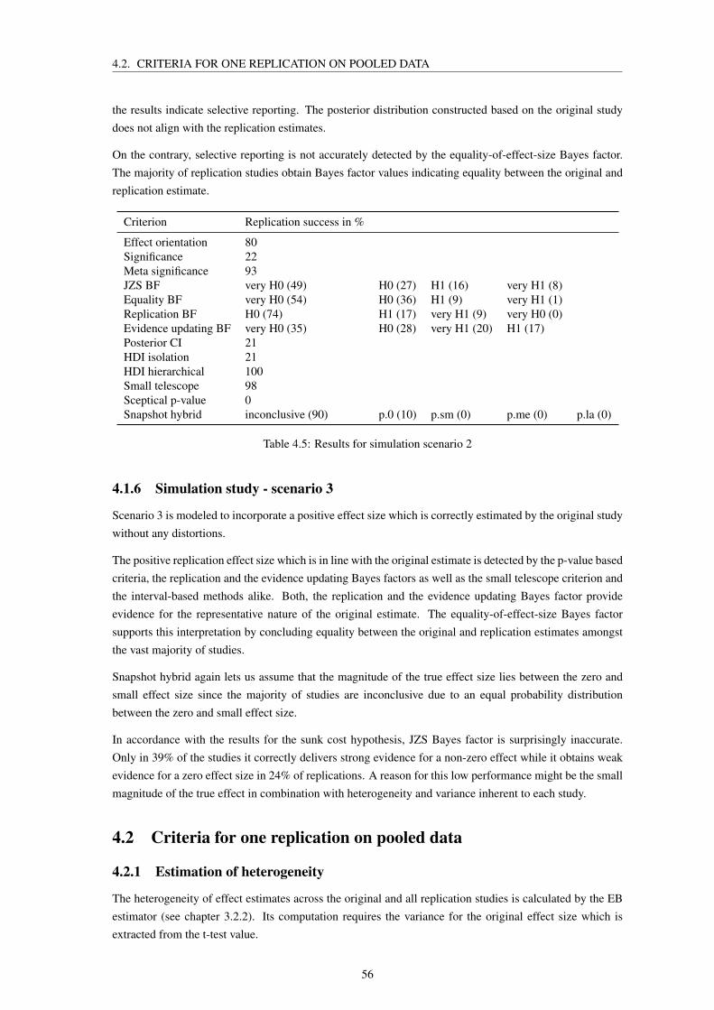
4.2. CRITERIA FOR ONE REPLICATION ON POOLED DATA

the results indicate selective reporting. The posterior distribution constructed based on the original studydoes not align with the replication estimates.

On the contrary, selective reporting is not accurately detected by the equality-of-effect-size Bayes factor.The majority of replication studies obtain Bayes factor values indicating equality between the original andreplication estimate.


Effect orientation 80Significance 22Meta significance 93JZS BF very H0 (49) H0 (27) H1 (16) very H1 (8)Equality BF very H0 (54) H0 (36) H1 (9) very H1 (1)Replication BF H0 (74) H1 (17) very H1 (9) very H0 (0)Evidence updating BF very H0 (35) H0 (28) very H1 (20) H1 (17)Posterior CI 21HDI isolation 21HDI hierarchical 100Small telescope 98Sceptical p-value 0Snapshot hybrid inconclusive (90) p.0 (10) p.sm (0) p.me (0) p.la (0)



Scenario 3 is modeled to incorporate a positive effect size which is correctly estimated by the original studywithout any distortions.

The positive replication effect size which is in line with the original estimate is detected by the p-value basedcriteria, the replication and the evidence updating Bayes factors as well as the small telescope criterion andthe interval-based methods alike. Both, the replication and the evidence updating Bayes factor provideevidence for the representative nature of the original estimate. The equality-of-effect-size Bayes factorsupports this interpretation by concluding equality between the original and replication estimates amongstthe vast majority of studies.

Snapshot hybrid again lets us assume that the magnitude of the true effect size lies between the zero andsmall effect size since the majority of studies are inconclusive due to an equal probability distributionbetween the zero and small effect size.

In accordance with the results for the sunk cost hypothesis, JZS Bayes factor is surprisingly inaccurate.Only in 39% of the studies it correctly delivers strong evidence for a non-zero effect while it obtains weakevidence for a zero effect size in 24% of replications. A reason for this low performance might be the smallmagnitude of the true effect in combination with heterogeneity and variance inherent to each study.

4.2 Criteria for one replication on pooled data

4.2.1 Estimation of heterogeneity

The heterogeneity of effect estimates across the original and all replication studies is calculated by the EBestimator (see chapter 3.2.2). Its computation requires the variance for the original effect size which isextracted from the t-test value.

56

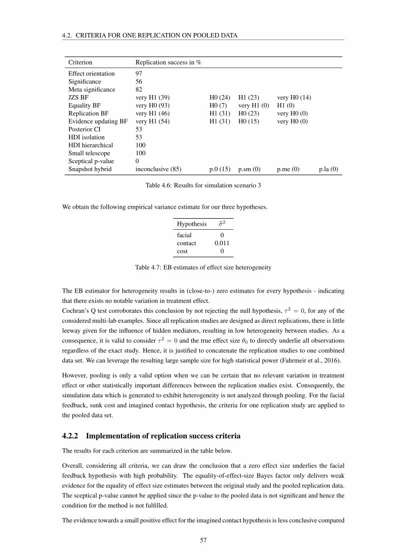
4.2. CRITERIA FOR ONE REPLICATION ON POOLED DATA


Effect orientation 97Significance 56Meta significance 82JZS BF very H1 (39) H0 (24) H1 (23) very H0 (14)Equality BF very H0 (93) H0 (7) very H1 (0) H1 (0)Replication BF very H1 (46) H1 (31) H0 (23) very H0 (0)Evidence updating BF very H1 (54) H1 (31) H0 (15) very H0 (0)Posterior CI 53HDI isolation 53HDI hierarchical 100Small telescope 100Sceptical p-value 0Snapshot hybrid inconclusive (85) p.0 (15) p.sm (0) p.me (0) p.la (0)


We obtain the following empirical variance estimate for our three hypotheses.

Hypothesis σ2

facial 0contact 0.011cost 0

Table 4.7: EB estimates of effect size heterogeneity

The EB estimator for heterogeneity results in (close-to-) zero estimates for every hypothesis - indicatingthat there exists no notable variation in treatment effect.Cochran’s Q test corroborates this conclusion by not rejecting the null hypothesis, τ2 = 0, for any of theconsidered multi-lab examples. Since all replication studies are designed as direct replications, there is littleleeway given for the influence of hidden mediators, resulting in low heterogeneity between studies. As aconsequence, it is valid to consider τ2 = 0 and the true effect size θ0 to directly underlie all observationsregardless of the exact study. Hence, it is justified to concatenate the replication studies to one combineddata set. We can leverage the resulting large sample size for high statistical power (Fahrmeir et al., 2016).

However, pooling is only a valid option when we can be certain that no relevant variation in treatmenteffect or other statistically important differences between the replication studies exist. Consequently, thesimulation data which is generated to exhibit heterogeneity is not analyzed through pooling. For the facialfeedback, sunk cost and imagined contact hypothesis, the criteria for one replication study are applied tothe pooled data set.

4.2.2 Implementation of replication success criteria

The results for each criterion are summarized in the table below.

Overall, considering all criteria, we can draw the conclusion that a zero effect size underlies the facialfeedback hypothesis with high probability. The equality-of-effect-size Bayes factor only delivers weakevidence for the equality of effect size estimates between the original study and the pooled replication data.The sceptical p-value cannot be applied since the p-value to the pooled data is not significant and hence thecondition for the method is not fulfilled.

The evidence towards a small positive effect for the imagined contact hypothesis is less conclusive compared

57

4.3. CRITERIA FOR MULTIPLE REPLICATIONS

to the sunk cost hypothesis. Nevertheless, the majority of criteria speak for a non-zero effect. However,the original effect estimate seems to have been subject to distortion in the form of selective reporting.This observation follows from the equality-of-effect-size Bayes factor which delivers weak evidence forinequality between the estimates. The result from the small telescope criterion also speaks for selectivereporting since the pooled replication estimate is not detectable.

The results for the sunk cost hypothesis speak for a small positive effect size which is significantly differentfrom zero. This is indicated by the significance of both p-value and meta-analysis p-value. The JZS andreplication Bayes factor both decisively speak for the alternative hypothesis. The small telescope criterionshows that the replication effect estimate could potentially be detected by the original study and henceconfirms the original significant effect estimate. The equality-of-effect-size Bayes factor concludes that theoriginal and pooled replication study align in their effect estimate and consequently that the original studywas not heavily influence by any distorting factors.

Criterion Facial Feedback Imagined contact Sunk cost

Effect estimate orientation FALSE TRUE TRUESignificance test: p-value 0.516 0.000 0.000Meta-analysis p-value 0.452 0.229 0.000JZS Bayes factor 5.000000e-02 1.883815e+04 8.440864e+23Equality-of-effect-size Bayes factor 0.731 1.215 0.091Replication Bayes factor 4.800000e-02 7.387137e+03 3.113805e+24Small telescope: significant (1) 1 1 0Sceptical p-value: p-value 0.480 0.475Snapshot hybrid p.0 (100) p.sm (100) p.sm (100)

Table 4.8: Results overview for replication success criteria applied to pooled multi-lab examples

The below graph 4.1 plots the 90% credibility interval for the posterior distribution in combination with theoriginal effect estimate for all three multi-lab examples. For the facial feedback hypothesis, zero is includedin the interval, implying a zero effect and hence non-replicability. For the two other multi-lab examples, theposterior equal-tailed credibility interval excludes zero, indicating the existance of an effect.

Overall, we can draw following conclusions,

- facial: The effect size is not significantly different from zero and the original estimate according toStrack et al., 1988 is an extreme overestimation of the true effect.

- contact: While a small non-zero effect seems to exist, the original effect estimate by Husnu and Crisp,2010 is an overestimation due to selective reporting.

- costs: We can observe a positive effect size, significantly different from zero and aligned with theoriginal estimate by Oppenheimer et al., 2009.

4.3 Criteria for multiple replications

The following section analyzes the outcome of applying the replication success criteria introduced in chap-ter 3.2.5. They are implemented on all available replication studies simultaneously. Therefore, they allowfor an overarching decision regarding replicability while acknowledging all conducted replication studies.

58


0.00

0.25

0.50

0.75

facial contact costsmulti−lab hypothesis

Coh

en's

d

original pooled replication

Figure 4.1: 90% credibility interval for the one-sided posterior distribution


In figure 4.2 Berkson’s interocular traumatic test for the facial feedback hypothesis lets us assume that thetrue effect size is either zero or close-to-zero. The original significant effect estimate is an overestimation,suffering under publication bias, and is consequently not replicable.

Bayesian evidence synthesis Bayes factor acc. to BayesFactor Bayes factor acc. to Wagenmakers

0.05 0.08 0.05

Table 4.9: Results for facial feedback hypothesis (arbitrary threshold value 1 billion, introduced for read-ability)

All three criteria speak for the null hypothesis. The observed data across all replication studies is morelikely to have been generated from a zero effect than a positive effect.


While Berkson’s interocular traumatic test in figure 4.3 implies a small non-zero effect, the original estimateseems to be subjected to selective reporting since it strongly overestimates the true effect size.


18838.15 216890.05 152096.38

Table 4.10: Results for imagined contact hypothesis (arbitrary threshold value 1 billion, introduced forreadability)

Again, all three criteria support the alternative hypothesis - a non-zero effect size. However, the evidence isless conclusive than for the sunk cost hypothesis.

4.3.3 Sunk cost hypothesis

For the sunk cost hypothesis, Berkson’s interocular traumatic test in figure 4.4 indicate a non-zero positiveeffect estimate for which the original estimate is an undistorted representation.

59


−0.5

0.0

0.5

5 10 15Study ID

Mea

n di

ffere

nce

Facial feedback

−0.2

0.0

0.2

0.4

5 10 15Study ID

Coh

en's

d

original replication

Figure 4.2: Overview: mean difference between condition and control group and Cohen’s d - facial feedbackhypothesis

−0.5

0.0

0.5

1.0

0 10 20 30Study ID

Mea

n di

ffere

nce

Imagined contact

−0.5

0.0

0.5

0 10 20 30Study ID

Coh

en's

d


Figure 4.3: Overview: mean difference between condition and control group and Cohen’s d - imaginedcontact hypothesis

60



> 1B > 1B > 1B

Table 4.11: Results for sunk cost hypothesis (arbitrary threshold value 1 billion, introduced for readability)

0.0

0.5

1.0

1.5

0 10 20 30Study ID

Mea

n di

ffere

nce

Sunk costs

0.00

0.25

0.50

0 10 20 30Study ID

Coh

en's

d


Figure 4.4: Overview: mean difference between condition and control group and Cohen’s d - sunk costhypothesis

All three criteria deliver decisive evidence for a non-zero effect size with very high Bayes factor values.


Berkson’s interocular traumatic test for simulation scenario 1 (in figure 4.5) - as well as for scenario 2 (seefigures 4.6) - is less conclusive. This exemplifies the limited detective and explanatory power of Berkson’stest and simple graphical visualization in general.

However, the overview of raw difference between condition and control mean as well as the effect sizemeasured as Cohen’s d illustrate an equal deviation around zero, indicating that the true underlying effectsize is zero. The original effect estimate is located at the boundary of observed values but there exist evenmore extreme values.


0.05 0.07 0.04

Table 4.12: Results for simulation scenario 1 (arbitrary threshold value 1 billion, introduced for readability)

For scenario 1, the criteria which we apply to all replication studies simultaneously conclude a zero effect.


As aforementioned, the Berkson’s interocular traumatic test for scenario 2 is rather inconclusive. Thedistribution of the effect size - measured as both mean difference and Cohen’s d - is skewed towards positivevalues, indicating a non-zero positive effect size. However, we cannot accurately identify distortion due toselective reporting since the effect estimates show substantial deviation.

61


−0.50

−0.25

0.00

0.25

0.50

0 25 50 75 100Study ID

Mea

n di

ffere

nce

Scenario 1

−0.2

0.0

0.2

0.4

0 25 50 75 100Study ID

Coh

en's

d


Figure 4.5: Overview: mean difference between condition and control group and Cohen’s d - scenario 1


> 1B > 1B > 1B


All three criteria provide evidence for the alternative hypothesis. This allows us to rightfully conclude anon-zero effect size underlying scenario 2 - without delivering any information on potential distortions.


Berkson’s interocular traumatic test for scenario 3 indicates that the original estimate is representative forthe estimates obtained in the replication studies. This lets us infer that the original study is likely to not havebeen subjected to any distorting factors. Its conclusion of a significant, positive effect can be consideredjustified.


> 1B > 1B > 1B


All three criteria deliver large Bayes factor values, rightfully exhibiting strong evidence for the alternativehypothesis.

4.3.7 Graphical summary: non-central confidence interval

Figure 4.8 shows replicability is not given for the facial feedback hypothesis but indeed present in the sunkcost and imagined contact hypothesis.

However, the lower limit to the confidence interval of the imagined contact hypothesis is in close proximityto zero. The confidence interval thus suggests an effect only slightly different from zero (Klein et al., 2014).

For scenario 1, the non-central confidence interval includes zero and hence rightfully concludes a zeroeffect. The original Cohen’s d estimate - plotted as dark green star - shows that the original estimate is

62


−0.3

0.0

0.3

0.6

0.9

0 25 50 75 100Study ID

Mea

n di

ffere

nce

Scenario 2

−0.2

0.0

0.2

0.4

0 25 50 75 100Study ID

Coh

en's

d



0.0

0.5

1.0

0 25 50 75 100Study ID

Mea

n di

ffere

nce

Scenario 3

0.0

0.2

0.4

0.6

0 25 50 75 100Study ID

Coh

en's

d



63

4.4. THE INFLUENCE OF A ONE-SIDED PRIOR DISTRIBUTION

0.0

0.3

0.6

0.9

facial contact cost scenario 1 scenario 2 scenario 3Data

Coh

en's

d

original replication truth

Figure 4.8: Non-central confidence intervals for Cohen’s d - multi-lab examples and simulation data

an overestimation of the true effect. The same can be observed for scenario 2, for which the discrepancybetween confidence interval and original estimate is even more distinct. Due to variation in treatment effect,the Cohen’s d estimate for the original study differs notably from the non-central interval for scenario 3despite it being simulated without distortions. For scenario 2 and 3, the non-central interval does not entailzero and hence allows the conclusion of a non-zero effect.

In general, the non-central interval seems a rather practical criterion since it allows a double assessment -whether the replication studies deliver evidence for a zero effect as well as what value the true effect size islikely to have. The accuracy of the latter can be illustrated by considering the true parameter sizes availablefor the simulation data. Plotting the median of the true Cohen’s d effect size for all scenarios (pink triangle)showcases the precise overlap between true value and constructed non-central effect size interval.

4.4 The influence of a one-sided prior distribution

4.4.1 One-sided priors for Bayes factors

While the equality-of-effect-size Bayes factor and the replication Bayes factor rely on a two-sided prior, theJZS Bayes factor, the evidence updating Bayes factor,evidence synthesis and the fixed effect meta-analysisBayes factor incorporate an oriented prior probability distribution which only attributes non-zero densitiesto positive effect size values.

In order to assess the influence of such a prior assumption, we have evaluated each of the one-sided criteriatwice - with and without the one-sided limitation.

The tables 4.15 to 4.20 illustrate the difference between the limited and unlimited implementations of eachcriterion - labelled ’(one)’ for the limited and ’(two)’ for the unlimited version.

The results for the criteria designed to be applied to one replication study at a time - JZS Bayes factor andevidence updating Bayes factor - are indicated as success rates in %. The results for the criteria assessingall available replication studies simultaneously - evidence synthesis and fixed effect meta-analysis Bayesfactor - are given directly as Bayes factor value.To ensure readability, Bayes factor values are cut off at an arbitrary threshold of 1 billion.

64


As aforementioned, the fixed effect meta-analysis JZS Bayes factor according to our self written code isnot identical to the Bayes factor calculated according to Wagenmakers, Beek, et al., 2016 due to differentapproximations.

Overall, no major changes in the outcome for any criterion can be observed. The interpretation regardingthe effect size for the multi-lab examples as well as the simulation study seem to be independent of the priorchoice.

Criterion Replication success

JZS BF (one) very H0 (76.5) H0 (23.5) H1 (0) very H1 (0)JZS BF (two) very H0 (82.4) H0 (17.6) H1 (0) very H1 (0)Evidence synthesis (one) 0.05Evidence synthesis (two) 0.052Meta-analysis BF (one) 0.076Meta-analysis BF (two) 0.056Meta-analysis BF (Wagenmakers) 0.046

Table 4.15: Bayes factor comparison for facial feedback hypothesis (arbitrary threshold value 1 billion,introduced for readability)


JZS BF (one) very H0 (47.2) H0 (27.8) H1 (13.9) very H1 (11.1)JZS BF (two) very H0 (55.6) H0 (30.6) very H1 (8.3) H1 (5.6)Evidence synthesis (one) 18838.154Evidence synthesis (two) 9419.079Meta-analysis BF (one) 216890.054Meta-analysis BF (two) 108445.029Meta-analysis BF (Wagenmakers) 152096.38

Table 4.16: Bayes factor comparison for imagined contact hypothesis (arbitrary threshold value 1 billion,introduced for readability)


JZS BF (one) very H1 (41.7) H0 (25) H1 (22.2) very H0 (11.1)JZS BF (two) very H0 (27.8) H1 (25) very H1 (25) H0 (22.2)Evidence synthesis (one) > 1BEvidence synthesis (two) > 1BMeta-analysis BF (one) > 1BMeta-analysis BF (two) > 1BMeta-analysis BF (Wagenmakers) > 1B

Table 4.17: Bayes factor comparison for sunk cost hypothesis (arbitrary threshold value 1 billion, introducedfor readability)

4.4.2 One-sided priors for posterior equal-tailed credibility interval

The posterior equal-tailed credibility intervals can also be constructed based on either a one-sided or atwo-sided JZS prior. The one-sided posterior credibility interval tests a directional alternative hypothesis,H1 : θ0 ≥ 0.

The resulting mean credibility intervals for the multi-lab examples and the simulation study are plotted infigure 4.9. The one-sided version (with a more shallow width) is on the left, the two-sided version (with awider width) is on the left for each hypothesis.

65



JZS BF (one) very H0 (75) H0 (20) H1 (3) very H1 (2)JZS BF (two) very H0 (78) H0 (18) H1 (3) very H1 (1)Evidence updating BF (one) very H0 (40) H0 (39) H1 (17) very H1 (4)Evidence updating BF (two) H0 (44) very H0 (36) H1 (16) very H1 (4)Evidence synthesis (one) 0.055Evidence synthesis (two) 0.032Meta-analysis BF (one) 0.069Meta-analysis BF (two) 0.039Meta-analysis BF (Wagenmakers) 0.035

Table 4.18: Bayes factor comparison for scenario 1 (arbitrary threshold value 1 billion, introduced forreadability)


JZS BF (one) very H0 (49) H0 (27) H1 (16) very H1 (8)JZS BF (two) very H0 (65) H0 (22) H1 (10) very H1 (3)Evidence updating BF (one) very H0 (35) H0 (28) very H1 (20) H1 (17)Evidence updating BF (two) very H0 (35) H0 (28) very H1 (20) H1 (17)Evidence synthesis (one) > 1BEvidence synthesis (two) > 1BMeta-analysis BF (one) > 1BMeta-analysis BF (two) > 1BMeta-analysis BF (Wagenmakers) > 1B



JZS BF (one) very H1 (39) H0 (24) H1 (23) very H0 (14)JZS BF (two) H0 (34) very H1 (28) very H0 (25) H1 (13)Evidence updating BF (one) very H1 (56) H1 (30) H0 (12) very H0 (2)Evidence updating BF (two) very H1 (54) H1 (31) H0 (15) very H0 (0)Evidence synthesis (one) > 1BEvidence synthesis (two) > 1BMeta-analysis BF (one) > 1BMeta-analysis BF (two) > 1BMeta-analysis BF (Wagenmakers) > 1B


The zero effect underlying the facial feedback hypothesis and scenario 1 is detected by the two-sided in-terval, not by the one-sided one. The two-sided interval is unable to observe the small non-zero effect inthe imagined contact hypothesis and scenario 2. However, the mean of the median of the effect estimatefor scenario 2 computed by the two-sided version is closer to the real mean effect size than the one-sidedversion.

For scenario 3, the one-sided mean estimate has lower bias to the true effect.

66


−0.3

0.0

0.3

0.6

0.9

facial contact costData

Coh

en's

d

Multi−lab examples

−0.2

0.0

0.2

0.4

scenario 1 scenario 2 scenario 3Data

Coh

en's

d

Simulation study

original replication truth

Figure 4.9: Posterior equal-tailed credibility interval with one- and two-sided JZS prior

67

4.5. ASSESSMENT OF ASSUMPTIONS

4.5 Assessment of assumptions

After implementing the criteria on the multi-lab examples and the simulation data, the question ariseswhether the initial assumptions adopted by the criteria (see chapter 3.2.2) are actually fulfilled.

For the simulation study scenarios both assumptions - normality and variance homogeneity - are guaranteedby the simulation process itself.

In the following, all three multi-lab hypotheses are analyzed regarding normality and variance homogeneitybetween condition and control group.

4.5.1 Assumption of normality

Whether the mean effect difference is normally distributed or not is determined graphically and numericallyleveraging

1. QQ-Plot

2. Shapiro-Wilks test: H0 : d ∼ N(µ, σ2)

The Shapiro-Wilks test results in non-significant p-values for each hypothesis. Consequently, the null hy-pothesis that the mean effect difference follows a normal distribution cannot be rejected.

Hypothesis p-value

facial 0.59contact 0.44cost 0.93

Table 4.21: Shapiro-Wilks test results

The points in the QQ-Plots lie more or less close to the bisection line and within the confidence interval forevery hypothesis, see plots 4.10.

The boundary quantiles of the imagined contact hypothesis divert from the bisection line and its confidenceinterval.

Both methods combined allow accepting the normality assumption of the effect size for all three hypotheses.

Several Bayes factor based criteria (e.g. JZS Bayes factor, replication Bayes factor) require the individualobservations in condition and control group across all replication studies to follow a normal distribution.This is assessed through visualizing the observations, separated for condition and control group, acrossall studies in a density plot. For the facial feedback and imagined contact hypothesis, the density plotproves a bell shaped distribution. For the sunk costs hypothesis, the normality assumption does not apply.The distribution seems to be suffering under a ceiling effect (Garin, 2014), showing that people are highlywilling to attend a game by their favorite soccer team despite bad weather and independent of the appliedtreatment. This could indicate that selecting soccer - an emotional sport for many (Jones et al., 2012) - forthe experimental set up is an unfortunate choice.

In conclusion, while the raw mean differences between condition and control group for the sunk cost hy-pothesis follow a normal distribution, neither the normality assumption for the individual observations northe variance homogeneity are fulfilled.

It has to be to pointed out that while the criteria in question model the individual data points to be sampledfrom a normal distribution, they only utilize the t-test in their explicit calculation (Rouder et al., 2009). It

68


−0.4

0.0

0.4

−2 −1 0 1 2Theoretical quantiles

Sam

ple

quan

tiles

Facial feedback

−0.5

0.0

0.5

1.0


Sam

ple

quan

tiles

Imagined contact

0

1

2


Sam

ple

quan

tiles

Sunk cost

Figure 4.10: QQ-Plot for multi-lab hypotheses

can be argued that the corresponding t-distribution is valid despite non-normality due to the central limittheorem (Fahrmeir et al., 2016, Ghasemi and Zahediasl, 2012).

4.5.2 Assumption of equal variance

The two-sample t-test as well as the criteria computing Bayes factors assume identical variance for conditionand control group. This assumption is guaranteed to be met for the simulation data.

For the multi-lab examples, the validity of the homogeneity assumption is assessed by plotting the differ-ence in variance between condition and control group, ∆, in figure 4.12 and by performing a FK test ofhomogeneity of variances.

For the facial feedback hypothesis, homogeneity in variance is assumed by Wagenmakers, Beek, et al., 2016and consequently maintained for our purposes. The difference in variance between condition and controlgroup for the imagined contact hypothesis lies within the same range as for the facial feedback hypothesis.Hence, the conclusion of homogeneity seems justified. This is also corroborated for both hypotheses bythe FK test. The overwhelming majority of replication studies - 0.941% for the facial feedback hypothesis,0.972% for the imagined contact hypothesis - result in an insignificant p-value to the significance level of0.05.

For the sunk cost hypothesis, ∆ tends to have negative values, indicating a heteroscedastic variance withhigher values in the control than in the condition group. However, positive differences do exist. The FK testobtains an equally inconclusive result. 0.472% of replication studies have an insignificant p-value, 0.528%a significant one.

In accordance with the other two multi-lab hypotheses and the inconclusive result, we assume variancehomoscedasticity for the sunk cost hypothesis.

69


0.0

0.1

0.2

0.0 2.5 5.0 7.5Rating: humor in cartoons

Den

sity

Facial feedback

0.00

0.05

0.10

0.15

0.20

2.5 5.0 7.5Likelihood: interaction with outgroup

Den

sity

Contact

0.00

0.25

0.50

0.75

2.5 5.0 7.5Likelihood: attendance of soccer game

Den

sity

Costs

Control Condition

Figure 4.11: Density plot for multi-lab hypotheses

−1

0

5 10 15ID

∆

Facial

−1

0

1

0 10 20 30ID

∆

Contact

−5.0

−2.5

0.0

2.5

0 10 20 30ID

∆

Costs

Figure 4.12: Difference ∆ in variance between condition and control group for multi-lab hypotheses

70

Chapter 5

Discussion

The aim of this thesis was to investigate the performance of selected criteria to define replication successin light of potential distortions and different true effect sizes. To do so, we implement the criteria on threemulti-lab examples as well as a simulation study including three scenarios. In order to explore the effects ofdistortions on the criteria, one example-scenario pair is affected by publication bias and another by selectivereporting. The third serves as a control instance and is uninfluenced by any distorting factors.

In the following chapter, we continue to discuss the performance of the selected replication criteria afterhaving embedded the result into the criticism given in the wider literature in chapter 4.

To recall, we are particularly interested in answering two questions:

1. Is there a zero effect and the original estimate an artefact of publication bias?

2. Is the original effect an overestimate due to selective reporting?

Hence, the assessment will in particular focus on each criterion’s performance when either publication biasor selective reporting is present.

5.1 Discussion of criteria for one and multiple replications

5.1.1 Criticism on frequentist criteria

If the true parameter is (close to) zero and multiple replication studies are available, the criterion of com-

paring the effect orientation can detect publication bias by indicated an approximately equal distributionof studies between same and different direction. However, it cannot account for selective reporting sinceneither the concrete effect size, nor any significant discrepancy from the original effect estimate is takeninto account. Simply comparing the signs of the estimates summarizes the information from the studiesrather rudimentary - it disregards too much of reality.

The p-value criteria - be it the simple p-value or the meta-analysis p-value - do not allow us to account forany distorting factors. Whether a study leads to a significant estimate is highly dependent on the samplesize - this contributes to the difference between p-value and meta-analysis p-value. The simple p-value alsooverestimates the evidence for the null hypothesis. Despite the fact that scenario 2 and 3 - as well as theimagined contact and sunk cost hypothesis - have a true non-zero effect size, at least a half of the replicationstudies obtain a non-significant p-value.

71

5.1. DISCUSSION OF CRITERIA FOR ONE AND MULTIPLE REPLICATIONS

There is increasing criticism from the scientific community against the use of p-values to define replicationsuccess - and to perform hypothesis testing in general - due to the many weaknesses elaborated in chapter3.2.4. The disadvantages of p-value based methods are well showcased in our analysis on the multi-labexamples as well as the simulation study. Relying on the p-values for decision-making leaves multipleopen questions. When the replication turns out non-significant, does that mean the original study was afalse-positive? Or is rather the replication study a false-negative (Laraway et al., 2019)? Deciding solelydepending on the replication p-value omits all evidence collected in the original study (Van Aert and VanAssen, 2017). The extent to which p-values can be interpreted as an objective and informative representationis questionable, in particular since they depend on sample sizes and the statistical power of tests. Both areparameters which vary across replications (Verhagen and Wagenmakers, 2014).

Overall, the p-value and null hypothesis significance testing are more limited and problematic in theirapplicability than their popularity and ubiquitous usage let us believe. Hence, there is increasing oppositionand lobbying against their widespread application and faulty interpretation (e.g. Goodman, 1999).

5.1.2 Criticism on Bayesian criteria

The JZS Bayes factor only exhibits a mediocre performance in determining replication success. As observ-able from the results obtained for the pair scenario 2 and imagined contact hypothesis, it is ill fit to detecta non-zero effect size if it is characterized by a small magnitude and within-study variance. Applying theJZS Bayes factor on the pooled data sets proves the dependence on sample size. The bigger the sample, themore likely the JZS Bayes factor is to pick up on small effects.

While the equality-of-effect-size Bayes factor can score with creating an explicit relationship between repli-cation and original effect, it is ill-equipped to detect distortions and handle variation in treatment effects.This can be observed in the results for scenario 1 and the facial feedback hypothesis as well as scenario 2and the imagined contact hypothesis. All parameters in said examples and scenarios are distorted by publi-cation bias and selective reporting. However, the equality-of-effect-size Bayes factor wrongly finds at leastweak evidence for equality between the replication and original estimate.

As aforementioned, the replication Bayes factor and its modification, the evidence updating Bayes factor,suffer from the so called replication paradox. This follows from the relative nature of its evidence (Lyet al., 2019) and is well illustrated in the results for scenario 2 and the imagined contact hypothesis - bothsubject to selective reporting. Despite a true non-zero effect size, the majority of Bayes factors exhibits atleast weak evidence for the null hypothesis. Despite the deviation from zero for the replication estimate,the posterior distribution in H1 explains the replication results worse than a distribution assuming a zeroeffect size. Consequently, the both Bayes factor versions are unsuited to determine replication success whenthe original study was subject to selective reporting. They perform better in detecting publication bias, asevident in the results for the facial feedback hypothesis. However, for scenario 1, the performance is lessconvincing. The replication Bayes factor and the evidence updating Bayes factor seem negatively affectedby heterogeneity.

When considering all replication studies simultaneously, the fixed-effect meta-analysis Bayes factor andBayesian evidence synthesis come to equal conclusions. Both criteria do not allow for any statistical explo-ration of the relationship between the original study and its replications but only to establish the existence -or non-existence - of a true non-zero effect.

72

5.1. DISCUSSION OF CRITERIA FOR ONE AND MULTIPLE REPLICATIONS

5.1.3 Criticism on interval-based methods

Testing whether the credibility interval constructed based on the posterior density of the effect entails zeroconstitutes a combination of frequentist null hypothesis testing and Bayesian statistics. The 90% credibilityinterval describes - as the name suggests - the co-domain in which the effect size lies with a probability of90%. We chose a significance level of 90% due to the one-sided nature of our analysis. We are interestedin estimating a lower boundary which will allow us to assess the proximity between the effect size andzero. In theory, we could construct a one-sided credibility interval with lower limit α = 0.05 quantile andupper limit infinity. However, the lower limit for the one-sided interval equals the lower limit of a two-sidedinterval with the significance level, α = 0.1. As a benefit to the two-sided interval, the upper limit at the1− α

2 quantile can be leveraged to detect overestimation in the original estimate (Fahrmeir et al., 2016).

Identifying random noise from a true non-zero effect is challenging. In this thesis, we mitigate the problemby rounding the lower and upper boundary to two decimal places.

We assume two-sided priors for all interval-based methods due to the danger of artificially skewing thecredibility interval. The comparison between a two- and one-sided JZS prior when constructing the poste-rior equal-tailed credibility interval in chapter 4.4.2 has indicated that a directional assumption in form ofa one-sided prior leads to an overestimation of the effect size. For both, scenario 1 and the facial feedbackhypothesis, it wrongfully concludes a significant non-zero effect. The effect estimates from multiple repli-cation studies scatter around zero. The one-sided prior causes the positive effect estimates - even thoughthey are positive due to random noise - to be interpreted as evidence for the alternative hypothesis.

For the truly non-zero effects in the remaing examples and scenarios, the one-sided prior draws the rightconclusions and adds certainty by delivering intervals with a more shallow width.

Consequently, one-sided priors should only be leveraged if we are convinced that the effect is positive. Ifwe are interested in establishing the existence of a non-zero effect size, a two-sided prior can be consideredmore appropriate.

Both the posterior credibility interval and the HDI in isolation perform inaccurately when a true positiveeffect is characterized by a small magnitude and accompanied by larger variance - as seen for the imaginedcontact and sunk cost hypothesis. The effect estimate incorporates too much uncertainty and hence theintervals have a large width. For scenario 2 and scenario 3, the performance is better. This can most probablybe traced back to the increased sample size and the consequent smaller variance for the effect estimator. Ingeneral, remedy to increase certainty is found by leveraging information across the replication studies. TheHDI based on a hierarchical model exhibit the shallowest width and middle point nearest to the true value.It uniformly concludes the correct effect estimate for all hypotheses and scenarios. Consequently, it shouldbe preferred to the alternative two interval-based criteria.

Distortions could be conveniently detected through either visually comparing the original and the replicationestimate or through testing whether the original estimate lies within the credibility interval.

One main discussion point resulting from the Bayesian nature of the interval-based criteria is the definitionof prior distribution. For the posterior credibility interval, we have opted for a one-sided prior, identicalto the one-sided JZS prior. The validity and usefulness of such assumption can be questioned and requiresfurther attention.

73

5.2. THE POWER OF THE BAYESIAN FACTOR AND SNAPSHOT HYBRID

5.1.4 Criticism on small telescope

The biggest disadvantage of the small telescope criterion is its reliance on classic frequentist hypothesistesting via p-values. Hence, small telescope can statistically only prove non-replicability - since it cannotaccept the null hypothesis which entails the replicability claim.

The implementation of the small telescope method on the simulation scenario 1 and the facial feedbackhypothesis indicates that the criterion is also unsuited to detect a true zero effect in the presence of withinvariance and heterogeneity. Even a small effect caused by random noise can obtain sufficient statisticalpower for the original study. The threshold of 33% is set extremely low, especially in comparison to theestablished target statistical power of 80%.

In addition, our analysis has shown that small telescope cannot identify selective reporting.

Overall, it seems as if the sceptical p-value is not well suited to detect non-zero effect sizes with the magni-tude and variance we are observing.

However, the performance of the small telescope criterion can only be restrainedly evaluated by the simu-lation study. To obtain sufficient statistical power, the replication study requires a 2.5 times bigger samplesize than the original study - a condition that is not fulfilled in any of the simulated scenarios and only fewof the multi-lab replication studies.

5.1.5 Criticism on sceptical p-value

None of the replication studies - neither in the multi-lab examples nor in the simulated data - obtained asignificant result when applying the sceptical p-value approach. The sceptical p-value seems unsuited forthe low correlation coefficients and the high variability inherent in our data.

Its applicability is strongly limited by its condition that both original and replication effect estimate arerequired to be significant. Especially the latter is very infrequently significant (e.g. Open Science Collabo-ration, 2015).

5.2 The power of the Bayesian factor and snapshot hybrid

Overall, Bayesian methods allow for more a meaningful and flexible interpretation of their results. Byreturning a Bayes factor or a posterior probability, Bayesian criteria provide evidence for and against thenull hypothesis while the ordinary frequentist methods prove absence of evidence - and not evidence ofabsence (Fahrmeir et al., 2016).

The Bayes factor can also better depict ambiguity in data when the obtained results speak neither for H0

nor for H1 convincingly (Verhagen and Wagenmakers, 2014). P-values, on the other hand, tend to overstatethe evidence for the alternative hypothesis when data is ambiguous, suffering under Lindley’s paradox.

However, some Bayesian methods fall short in detecting selective reporting and publication bias (replica-tion Bayes factor and evidence updating Bayes factor) and in accounting for variation in treatment effects(equality-of-effect-size Bayes factor).

The comparisons between Bayes factors relying on either a one-sided or two-sided prior distribution inchapter 4.4.1 have illustrated that the two-sided version tends to interpret evidence more in favor of thenull hypothesis than the one-sided one. This follows from the relative nature of the Bayes factor. Sincethe examined effects for the imagined contact and sunk cost hypothesis as well as scenario 2 and 3 have

74


a positive size, the alternative hypothesis assuming a-priori distribution which equally attributes non-zeroprobabilities to positive and negative effect sizes matches the data as inaccurately as the null hypothesis. Itis hence a choice of the lesser evil. The one-sided prior distribution correctly modeling the positive sign ofthe effect matches said data better and is therefore accepted with a higher rate.

The comparison between one- and two-sided priors illustrates well why customizing the prior distributionaccording to the prior knowledge available of the effect is an essential step when implementing Bayesianmethods. It optimizes performance and allows for a more detailed explanation of the underlying researchtheory.

We consider the snapshot Bayesian hybrid meta-analysis method by Van Aert and Van Assen, 2017 a verypromising criterion. In a nutshell, it calculates the posterior probability for an effect of a certain size giventhe replication study data and the original data. If the posterior probability for a certain effect size lies abovethe threshold of 75%, we consider it substantial evidence for the effect size to be the true effect. The defaulteffect sizes tested in snapshot hybrid are a zero effect (0), a small effect (0.1), a medium effect (0.3) and alarge effect (r = 0.5).

Prior distributionThe default priori distribution is non-informative, i.e. each choice is allotted equal probability beforehand.Van Aert and Van Assen, 2017 prove that informative subjective prior probabilities can be easily incor-porated into the snapshot hybrid method without having to repeat the entire calculation process. Priorprobabilities can either remain discrete or can also be indicated in the form of a continuous distribution.Overall, snapshot hybrid has great flexibility in integrating prior assumptions regarding the potential effectsize (Van Aert and Van Assen, 2017).

Discrete effect size valuesAnother criticism is the limited number of distinct effect size choices. This is especially disadvantageouswhen the true effect size lies between two given choices. In such situations, snapshot hybrid will deliverapproximately equal evidence for both effect sizes - rendering a conclusive decision impossible. Thisphenomenon can be observed when applying snapshot hybrid to the sunk cost and imagined contact data aswell as scenario 2 and 3 .

However, the principle of snapshot hybrid is independent of the number and magnitude of effect size op-tions. In theory, they can be arbitrarily chosen by the researcher. We can regard this selection as the crite-rion’s subjective component in accordance with the subjective prior choice in Bayesian methods. Based onexpert knowledge, the researcher can hypothesize probable effect sizes and calculate their posterior prob-abilities based on replication and original data (Van Aert and Van Assen, 2017). The effect sizes testedin snapshot hybrid might also be set to values which impose some sort of relevance in the specific field -comparable to the dual-criterion design (Rosenkranz, 2021).

Identical sample sizesOne of the criticized points of snapshot hybrid is its inherent assumption of same sample sizes acrossreplication and original paper. The authors of snapshot hybrid have developed a web application van Aert,2021a in which unequal sample sizes for original and replication study can be incorporated. This feature issadly not available in the R function snapshot() available in the puniform package (van Aert, 2021b).

Assumption of homogeneity and increase of sample size through poolingSnapshot hybrid cannot account for any heterogeneity of the true effect size between original and replica-tion study but rather considers all replication studies to be identically and independently drawn from oneoverarching distribution (Van Aert and Van Assen, 2017). As our analyses have indicated, there is hardly

75


−0.25

0.00

0.25

0.50

contact cost facial scenario 1 scenario 2 scenario 3Data

corr

elat

ion

zero effect (0)

small effect (0.1)

medium effect (0.3)

large effect (0.5)

prediction

original estimate

effect size prediction / original

Figure 5.1: Correlation coefficients for all datasets and default effect sizes for snapshot hybrid

any measurable and certainly no significant heterogeneity in the multi-lab examples. Thus, the neglect ofheterogeneity in snapshot hybrid can be justified. As a consequence, data across replication studies can beconsidered to originate from one overarching distribution, allowing us to pool the data.

Snapshot hybrid requires big sample sizes for sufficient statistical power - e.g. a sample size of 300 to 1000to achieve 80% statistical power with a zero or small true effect size. Hence, the probability of inconclusiveresults is quite high for the combination of small sample size and small true effect size, customary in certainresearch areas (Van Aert and Van Assen, 2017). Pooling data serves as a remedy. Multiple smaller repli-cation studies are combined to one large data set providing high statistical power when applying snapshothybrid (Van Aert and Van Assen, 2017).

Ambiguity of dataSnapshot hybrid only considers posterior distributions over the threshold of 75% substantial evidence for acertain effect size. Other results are regarded inconclusive. Hence, snapshot hybrid accounts for ambiguityof data comparable to Bayes factors. It does not create a wrong sense of security as do other criteria, e.g.p-value significance (Van Aert and Van Assen, 2017).

Relationship between original and replication effect size estimateSnapshot hybrid takes the original data set into account when calculating the posterior distribution. It addi-tionally allows a comparison between the most likely effect estimate and the original estimate. Publicationbias would result in a zero effect size as a prediction from snapshot hybrid while the original estimatehas some positive significant effect. We can detect selective reporting if the predicted effect size based onsnapshot hybrid has a lower value than the original estimate. This analysis can be guaranteed by choosingcorresponding snapshot levels beforehand (Van Aert and Van Assen, 2017).

76

5.3. THE STRENGTH OF CONFIDENCE AND CREDIBILITY INTERVALS

5.3 The strength of confidence and credibility intervals

Several authors emphasize that a single or a small number of replication studies do not provide enoughinformation to determine replicability (e.g. Amrhein et al., 2018). Consequently, it is of great relevance toprovide statistical criteria which determine replication success based on several replication studies simulta-neously. However, the research for this thesis has primarily discovered methods for one replication studyand only few designated for multiple. Even the multi-lab analysis experiments conducted by e.g. Wagen-makers, Beek, et al., 2016 and Schweinsberg et al., 2016 predominantly apply criteria for one replicationstudy on all available replication studies individually.

If a limited number of replication studies are conducted, visual analysis methods are quick to apply, simpleto comprehend and often surprisingly expressive.

Berkson’s interocular traumatic test allows an easy assessment of publication bias and selective reporting.For both types of distortion, the original effect estimate lies at the outer edges and might even be consideredan outlier.

Nevertheless, visual exploration can only be the first step in conducting a more thorough inference of theeffect estimates across replication studies.

The construction of the non-central credibility interval combines the strengths of visualization with statis-tical inference. It enables detecting distortions due to publication bias and selective reporting as well asdetermining the most realistic empirical effect estimate - all well founded in a non-central t-distribution forthe raw mean difference θ. However, its construction relies on pooling the data. Hence, it disregards allheterogeneity between replication studies. While this does not have any effects on the multi-lab examplessince their heterogeneity is insignificant, it might render the criterion less suited to the simulation data anddata with high variation in treatment effects in general.

An alternative method which incorporates heterogeneity is the HDI in a hierarchical model. Averaging thelower and upper limit as well as the median across all available replication studies leaves us with one overallinterval. The HDI has the advantage of being a Bayesian credibility interval and with that in particular aneasy and intuitive interpretation.

5.4 Success or failure - criticism of a binary classification

In the context of this thesis, we consider replication studies as either successful or unsuccessful. Severalresearchers (e.g. Gelman, 2018, Amrhein et al., 2018) have pleaded to substitute such binary classificationwith continuous measurements of how much the replication corroborates the original findings. Gelman,2018 argues that instead of a binary classification researchers should “express the difference between oldand new studies in terms of the expected variation in the treatment effect between conditions” (no pageavailable). Anderson and Maxwell, 2016 even go so far as to claim that “[p]art of the reason for the crisisof confidence may be [...] viewing replication as a black and white dichotomy” (p.10). It is certainly truethat a criterion which only performs binary classification - e.g. comparison of effect estimate orientation, p-values - oversimplifies the complex question of establishing replicability. While this might discredit certainmethods it does not invalidate binary classification itself. We argue that the problem does not lie withinthe classification into success or failure to replicate per se but rather within the implementation of certaincriteria that classify replication studies in a binary matter.

While we do acknowledge that scientific findings are never black-or-white, we are convinced that scientificfindings require a deterministic element. A study is either replicable or not replicable within a certain

77

5.5. LIMITATIONS AND FURTHER INVESTIGATION

context - replicability is an all-or-nothing feature. Consequently, we hold on to a binary classification as thefinal conclusion when implementing the replication criteria.

Nevertheless, binary classification and continuous measurement of evidence for or against replicability arenot mutually exclusive. The continuous measurement is utilized to perform classification and serves asvaluable additional information acknowledging the uncertainty inherent to statistical inference. Essentialfor a theoretical interpretation of the research hypothesis in a wider sense is the binary classification.

Therefore, the focus should lie on applying metrics which identify replicability despite distortions and canbe leveraged to classify a study as success or failure with high accuracy.

5.5 Limitations and further investigation

This thesis aims to provide a first step towards a systematical review of criteria which can be utilized todefine replication success. While it is by no means an exhaustive investigation, the analysis of three multi-lab examples and three corresponding simulated scenarios allow an initial assessment of which criteriaperform better given an arbitrary effect size and accommodate potential distortions - publication bias andselective reporting.

In future work, the selected criteria should be applied to more multi-lab examples and simulation scenarios.This would not only further consolidate the initial evaluation but also determine the performance in light ofother distorting factors - such as p-hacking or HARKing. Throughout this thesis, we focused on publicationbias and selective reporting in the interpretation and assessment of criteria performance. However, it iseither impossible or very challenging to differentiate between distortion factors. Hence, the discrepanciesbetween the original study and its replications encountered in our analysis might potentially originate fromother influencing factors than interpreted. In order to further investigate distortions and their varying impacton the performance of replication criteria in more detail, more elaborate simulation studies are required(Hoffmann et al., 2020).

Thereby, we should also check for heterogeneity between replication studies to establish the prevalence ofcontext dependency in multi-lab data and the influence it has on the different criteria.

How the individual method behaves given different values for the effect size, for the variance within a studyand for the sample size can be examined by performing a more thorough simulation study in which theseparameters are systematically varied across a range of reasonable options and combinations.

Throughout the thesis, we have touched upon the issue of sufficient sample sizes for the replication studiesto obtain high statistical power for the respective criterion. Future work should further examine and comparethe required size for substantial statistical power between criteria and hence investigate the practicability ofthe respective methods.

While the replication crisis is an interdisciplinary phenomenon, we assume the biggest, most effective andmost sustainable impact is achieved when provided solutions are catered to the individual requirements,circumstances and idiosyncrasies of specific research fields. Hence, future reviews might incorporate areaspecific assessments and practical instructions on how to apply the replication criteria in day-to-day re-search.

78

Chapter 6

Conclusion

6.1 Suggestions and alternatives for the statistical evaluation of repli-cation success

6.1.1 Replication report

Throughout this thesis, we have established the paramount importance of conducting replication studies.Different statistical criteria on how to define replication success have been applied to multi-lab examplesand simulation data, analysing their suitability to handle potential distortion (selective reporting, publicationbias).The explicit purpose behind a replication study can be manyfold. “[R]eplication should be viewed as aconstruct that can be amenable to varying purposes and flexible in answering the questions that are mostbeneficial to moving [a] field forward in the domain of interest” (Anderson and Maxwell, 2016, p.10).Consequently, the various statistical approaches explore replicability in a different light. They containdifferent underlying conditions and assumptions, suffer from different weaknesses and shortcomings andanswer different questions (Anderson and Maxwell, 2016, Verhagen and Wagenmakers, 2014). One methodhardly suffices to grasp the complexity inherent to replication studies and can only be compared to othercriteria to a certain extent.

Therefore, Marsman et al., 2017 argue “that future analyses of replication studies will be more inclusive byemploying a range of different, complementary techniques.” (p. 16)Neither the criteria - if potential adaptions for multiple testing are considered - nor the purposes of testing areexclusive. Several criteria can and should be implemented simultaneously (Anderson and Maxwell, 2016).Including multiple replication metrics in “a comprehensive and coherent replication report” (Verhagen andWagenmakers, 2014, p. 1469) will allow us to paint a more accurate and nuanced picture of replicability.

As discussed in chapters 5.1 and 5.3, the snapshot Bayesian hybrid meta-analysis method as well as thenon-central confidence interval and the hierarchical credibility interval are considered promising and wellequipped to conclude replicability despite publication bias and selective reporting. Hence, we would rec-ommend incorporating them in the replication report.

79

6.1. SUGGESTIONS AND ALTERNATIVES FOR THE STATISTICAL EVALUATION OFREPLICATION SUCCESS

6.1.2 Alternative approaches

The scope of methods described and analysed in this thesis is by no means exhaustive. Throughout thethesis, we limit ourselves to a one-sided t-test. Evidently, most methods can be expanded to incorporateother test statistics.

Of course, an abundance of alternative criteria to assess replication success exists in the frequentist as wellas in the Bayesian framework. The interested reader might refer to Anderson and Maxwell, 2016 whoidentify six potential goals a replication study can pursue and give an extensive overview of methods thatcan be implemented to achieve each goal.

Beyond the existence of non-zero effectsSimonsohn, 2015 explains that “effects obtained in replication studies are currently evaluated almost exclu-sively on the basis of whether or not they are significantly different from zero.” (p. 560) This also applied tothe methods selected here. The majority of methods implemented in this thesis focus on assessing whetherthe replication study also indicates a true effect size that is significantly different from zero. However, thisis only the first step. Our interest in effects expands from the simple question of existence to its actual size.Only the equality-of-effect-size Bayes factor by Bayarri and Mayoral, 2002, the replication Bayes factorby Verhagen and Wagenmakers, 2014 and its extension by Ly et al., 2019 as well as the snapshot hybridmethod by Van Aert and Van Assen, 2017 allow more concrete conclusions on effect size than a simpleclassification into zero and not zero.

The replication crisis has showcased that empirical effect size estimates are subject to multiple distortingfactors, leading to a systematic overestimation (e.g. Zwaan et al., 2018) While establishing the existence- or non-existence for that matter - of an effect is important, it is also of great interest to explore howreplication studies can augment the accuracy in estimating the effect sizes. This is challenging - Van Aertand Van Assen, 2017 explain that “it is hard to obtain conclusive results about the magnitude of the trueeffect size in situations with sample sizes that are illustrative for current research practice.” (p.14) Some ofthe methods proposed in this thesis make a good start and show great potential for further development.

6.1.3 Essential role of preregistration and disclosure

What has been neglected so far are the prerequisites necessary to perform a replication study - proper ex-perimental logging and disclosure (Plesser, 2018, Nelson et al., 2018). Methodological approaches in datagathering and analysis have to be recorded to the extent of enabling other researchers to retrace the stepsand reproduce original experiments (Zwaan et al., 2018). Additionally, full disclosure of the detailed resultsincluding all performed measures and exclusions is required (Nelson et al., 2018).Vazire, 2018 points out that increased transparency in reporting experimental set-up, methods of data anal-ysis and all results will play a essential role in guaranteeing replicability. Only by making studies moreaccessible through meticulous reporting can researchers comprehend and trust findings. Brandt et al., 2014has provided a detailed replication recipe which instructs researchers on how to log their studies sufficiently.

One major remedy for HARKing and P-hacking is preregistration. Marsman et al., 2017 include prereg-istration as part of the “trinity of replication” (p. 2) next to collaboration with the original authors andhigh-powered studies.According to Center for Open Science, 2021, over 280 scientific papers have adopted preregistration in theform of registered reports. A registered report is handed to the publishing paper prior to conducting thestudy, explaining the scientific hypothesis and respective study design as well as the planned data analy-sis and predicted results (Nosek and Errington, 2017, Vazire, 2018). This registered report is then peerreviewed, focusing not on the outcome of the study but its methodological correctness, and accepted for

80

6.2. CURRENT SITUATION AND OUTLOOK

publication. The publication of the study is therefore guaranteed independent of the final outcome andcan only be revoked in case of concerns regarding quality and inexplicable procedural deviations from thepreregistered approach.

6.2 Current situation and outlook

6.2.1 Concerns regarding replicability

The replication crisis and its inert accusations of poor science - unintentionally made but perceived as such(Zwaan et al., 2018) - have created a heated debate and considerable controversy in the scientific community(e.g. Zwaan et al., 2018, discussion between Ioannidis, 2005, Ioannidis, 2007 and Goodman and Greenland,2007, discussion between Jager and Leek, 2014a, Jager and Leek, 2014b and Ioannidis, 2014).

Zwaan et al., 2018 enumerate some of the concerns regarding replicability as such, its assessment throughvarious statistical criteria and its practicability in the scientific day-to-day.

Variability in contextAs mentioned before, many argue that one main reason for lacking replicability in research is change incontext - be it due to time passed since the original study, geographical differences or other tacit factors.

In the context of one of the research hypothesis - the facial feedback hypothesis - utilized in this thesis, theoriginal author Strack, 2016 strives to undercut the evidence delivered by Wagenmakers, Beek, et al., 2016through replication studies. By questioning if the cartoons which were used in the study and “were iconicfor the zeitgeist of the 1980s instantiated similar psychological conditions 30 years later” (p.929), Strack,2016 suggests the reason for non-replicability is merely historical change and not the non-existence of theeffect described in Strack et al., 1988.

The danger behind this assumption of context variability is that it “renders the original theory unfalsifiable”(Zwaan et al., 2018, p. 6). Any failed direct replication study can be explained by deeming missing fea-tures post-hoc as essential to reproducing the effect. This attitude indicates wrongful hierarchical thinking,positioning the original study as more truthful or trustworthy than any replication study - without any justi-fication but simple sequential ordering. In the logic of the critics, rejection results in a new, more specifichypothesis which embeds the effect in an increasingly complex context dependency. Every one of theserefinements in hypothesis leads to more mediators added to the list of factors that must be included in areplication study (Klein et al., 2014). Following the theory of sophisticated falsificationism by Lakatos,1970, aforementioned briefly, the study becomes degenerative. It is caught up in a “fruitless cycle of con-stantly invoking auxiliary hypotheses that fail to garner support” (Zwaan et al., 2018, p. 6) and are ideallydismissed as wrong (Nosek and Errington, 2017, Musgrave and Pigden, 2021). However, the custom ofdenying non-significant studies has factually lead to “virtually unkillable” theories (Ferguson and Heene,2012, p. 559).The importance of replicability as a method of falsification has to be acknowledged without finding a per-manent excuse for failed replication in context dependency.

Limited value of direct replicationsAnother critical point held against direct replications in particular is its seemingly limited value creation.Eden, 2002 claims that the more original and replication study differ from each other, the higher the addedvalue and potential insight created by the replication study. Direct replications either succeed or fail intheir goal to replicate the original significant effect. Neither do they apply a new method, nor explore thehypothesis in a new setting, as conceptual replications do. Zwaan et al., 2018 argues that this perception

81


of direct replications not providing any new scientific discoveries is only valid as long as the significantoriginal effect was in fact true. Given the current replication crisis and the conclusive evidence for missingreplicability in many studies (e.g. Ioannidis, 2005, Open Science Collaboration, 2015), there is sufficientreason to doubt so. Conceptual replication has to, therefore, be replenished with direct replication to allowfor a wholesome verification of a hypothesis (Zwaan et al., 2018).

Replication as a wrong focal pointSeveral voices in the scientific community (e.g. F. Schmidt and Oh, 2016) can be heard stating that thereplication crisis should be less concerned with replication and more focused on other distorting factors -namely publication bias and questionable research practices (Zwaan et al., 2018). Overcoming these issueswould solve the current crisis, so the argument. We disagree with this position. Firstly, distortion factors areembedded in the wider discussion surrounding replicability and while they might heavily contribute, they donot reflect the entire complexity underlying the replication crisis. Secondly, simply changing nomenclaturehas neither measurable impact nor does it support a holistic approach towards a solution to the replicationcrisis. Nevertheless, we admit that replication is “just one element of the toolbox of methodological reform”necessary for change (Zwaan et al., 2018, p. 9).

Confidence in wrong methodologyDirect replication studies per definition repeat the original study in its methodological approach. Of course,a central condition for their validity is the statistically justified and correct implementation of the approach.As illustrated in Rotello et al., 2015, an analysis performed in the original study can be unsound and leadto flawed results. Replicating such studies and repeating the misleading methodologies could consequentlyincrease confidence in the wrong study results. According to Rotello et al., 2015, checking statistical as-sumptions before applying statistical methods to data is equally important as replicating studies. We wouldargue that ensuring a mathematically sound and correct implementation of test statistics is an irrefutableand even more fundamental component of good scientific practices than replicability. Therefore, whetherall relevant assumptions are met has to be considered separately from the test for replicability.

6.2.2 Consequences of the replication crisis - in public and science

The effects of the replication crisis on the scientific community have been manyfold - some call it a “re-naissance” (Nelson et al., 2018), some a “revolution” (Spellman, 2015). Others deny its existence or down-play its relevance (e.g. Stroebe and Strack, 2014). Again others see it as a degradation of science to a’paint-by-numbers’ process - simply reproducing studies by instructions instead of discovering new effectsindependently.

As the previous section 6.2.1 has hopefully indicated to the reader, the concerns regarding replicability, itsexact definition and its relevance are abundant.

Fact is that the replication crisis justifiably questions the quality of research as a whole. Therefore, it has im-plications for science as a whole. It has endangered the societal stance of science and has diminished publictrust and confidence in scientific findings and scientific expertise in general (German Research Foundation,2017). The lack of replicability also undermines the responsibility of science to serve as a foundation forinformed political decision making (Wingen et al., 2020). Consequently, conducting replication studies inthe public eye is essential to enhancing the believability of science and to regaining trust in the scientificprocess (Laraway et al., 2019).

What will the tangible effects of the new sense of alert for replicability on researchers be? Heated debateshave erupted and divided the scientific community (Chawla, 2016). It revolves around questions like,

82


- How many times must or should a study be replicated?

- When can a study be accepted as proven and how can research make new discoveries while concen-trating on replicability?

Baumeister, 2016 and Vazire, 2018 agree that while science will become more sustainable in the sense thatfindings will be more substantial and replicable, the ingenuity and creativity of researchers might suffer.Replicability could be perceived as a hindrance, inducing researchers to be more risk-adverse and lessbold in defining their hypothesis. Dorothy Bishop, a developmental neuropsychologist at the University ofOxford, even goes as far as to tweet, “the opposite of the reproducibility crisis! Stasis” (Chawla, 2016).

However, publishing false positive or overestimated effects is not much of scientific progress either.Throughout this thesis, we have established the importance of replication studies - from a philosophical,societal and statistical viewpoint. While we have mainly focused on the latter and the more practical aspectsof replication - how to statistically determine replication success - the replication crisis has to be consideredas a wider, more complex phenomenon. It is a symptom of many shortcomings - not only by researchersand publishers. The public perception of science also pays a great contribution to it.

6.2.3 The battle against the myth of science

The public is suffering from the myth of science, i. e. the impression that scientific findings are certainand true and once established they are accepted by the scientific community for eternity. Researchers aresuffering from the “myth that a scientist can do a perfect study” (Hunter, 2001, p. 151). For the public andthe research community alike, science is understood to ask questions and finds answers without a shadowof a doubt (Gelman, 2015a).

This idealistic understanding of science and scientific studies neglect scientific reality. Science has alwaysbeen shaped by new discoveries but also by self-improvement and self-correction. It is an evolving system ofexploring, gaining new knowledge and testing established facts - all in the eternal quest for truth (Simmonset al., 2011). However, this truth cannot be determined with complete and unconditional assurance throughstatistical analysis - since statistics does not equal reality. Unfortunately though, statistics is the only toolavailable to capture at least some of reality (Białek, 2018). Statistical inference is a “thought experiment”(Amrhein et al., 2018, p. 2) assuming a simplified version of reality to construct models and draw predictiveconclusions. Neglecting some of reality’s complexity is essential to fit statistical models with a limitedamount of data. Hence, as Vazire, 2018 summarizes, “error is inherent to the scientific progress” (p. 415)and uncertainty in the form of random sampling error or systematic distortion error will always remain.

However, this discrepancy between reality and statistics is all too often forgotten in science communica-tion. Positioning scientific findings as absolutely certain leads to inevitable and profound misunderstanding(Gelman and Carlin, 2017). Therefore, the replication crisis might be perceived not as a crisis of scienceand scientific conduct but rather as a crisis of scientific communication, a denial of scientific uncertaintyand an overestimation of statistical inference (Amrhein et al., 2018).

Consequently, researchers need to develop and practice a better and more veridical communication for theirfindings such that they are accessible to the layman (Laraway et al., 2019). This will empower the widerpublic to recalibrate their definition of science and accept uncertainty as one of its unavoidable components- and not as a sign of “junk science” (Białek, 2018, p.2, and Gelman, 2016).Simultaneously, researchers have to contemplate their fundamental values shared across fields - the valueof self-correction in light of unavoidable scientific error (Amrhein et al., 2018).

Only with an holistic approach including a shift in statistical practices as well as in mindsets will the

83


replication crisis be effectively and sustainably overcome. We are currently standing at the brink of afundamental methodological and cultural transformation - to rejoice in an age of ’replication renaissance’.To quote Nelson et al., 2018, “it is clear that the Middle Ages are behind us, and the Enlightenment is justaround the corner.” (p. 529)

84

Appendix A

Mathematical and statisticalfoundations

A.1 Fundamental empirical estimators

The empirical mean is computed by

x =1

n

n∑i=1

xi (A.1)

The within study variance is computed by

s2 =1

n− 1

n∑i=n

(xi − x)2 (A.2)

If the sample includes two groups, we frequently require the pooled variance

s2p =

1

n1 + n2 − 2

(s2

1 · (n1 − 1) + s22 · (n2 − 1)

)(A.3)

which is calculated based on the variance estimate and sample size for both groups respectively.

The standard deviation is the square root of the variance

sp =√s2p (A.4)

The covariance between two random variables X and Y is computed by

sXY =1

n− 1

n∑i=1

(xi − x) · (yi − y) (A.5)

85

A.2. COCHRAN’S Q TEST

A.2 Cochran’s Q test

Cochran’s Q test is a popular statistic to test for heterogeneity between effect sizes across studies. It estab-lishes whether a significant non-zero variance in treatment effect, τ2, exists

H0 : τ2 = 0 (A.6)

It is calculated based on the empirical effect size and standard error estimates, θi and si, for allm replicationstudies and one original study

Q =

m+1∑i=1

wi · (θi − θw)2 (A.7)

where θw denotes a weighted mean of the mean difference estimator, θi. The weights are determined by thereciprocal of the corresponding variance wi = 1

σ2i

θw =

∑m+1i=1 wiθi∑m+1i=1 wi

(A.8)

Since σ2i is unknown, we estimate wi = 1

s2i(Hoaglin, 2016).

Under the null, Q is assumed to follow a χ2 distribution with m degrees of freedom (Borenstein et al.,2021).

However, Hoaglin, 2016 argues that the Q statistic was not designed by its inventor, William G. Cochran,to test for heterogeneity and is hence unsuited to be used as such.

Nevertheless, Cochran’s Q statistic enjoys great popularity and will be leveraged in this thesis to establishheterogeneity between the original and replication effect size estimates.

A.3 Correlation

Correlation is an alternative method to measure effect size (Borenstein et al., 2021). Its benefits includebeing bound by an upper and a lower limit, its wide popularity and hence accessible interpretation (OpenScience Collaboration, 2015).

Correlation indicates how accurately one of two continuous variables X and Y can be explained as a lineartransformation of the other, i.e.

Y = a ·X + b (A.9)

The two variables run together: if one increases, the other one either increases (a > 0) or decreases (a < 0)proportionally.

Correlation is empirically measured by the Bravais-Pearson correlation coefficient. The covariance betweenthe two variables is divided by their respective standard deviations

ρXY =σXY

σX · σY(A.10)

The approximation depends on the empirical estimate of the covariance, sXY , between X and Y and the

86

A.4. FISHER TRANSFORMATION

empirical variance estimate for X and Y (Fahrmeir et al., 2016)

ρXY =sXYsX · sY

(A.11)

The correlation coefficient lies within the range [−1, 1]. It takes the values of the boundary if the relationshipbetween X and Y is perfectly linear. The less a linear relationship matches the data, the closer to zero thecorrelation coefficient is (Fahrmeir et al., 2016).The variance to the Bravais-Pearson correlation coefficient ρ depends on the estimate itself and the samplesize (Borenstein et al., 2021)

σ2ρ =

(1− ρ2XY )2

n− 1(A.12)

According to Borenstein et al., 2021, the empirical Cohen’s d estimate, d, which describes the effect of onevariable on the other, can be leveraged to determine the correlation coefficient

ρXY =d√

d2 + a(A.13)

If the sample sizes of the condition and control group are known, we insert

a =(ncond + nctr)

2

ncond · nctr(A.14)

If the exact distribution is unknown, we assume equal group sizes and hence a = 4 (Borenstein et al., 2021).

While establishing correlation requires two continuous variables, measuring a certain variable X in a di-chotomous experiment - consisting of a condition and control group - only provides one. Consequently,we assume that a continuous variable Y underlies the allocation to either control or condition group. Thisallows us to follow the established interpretation: if X increases, the hidden Y either increases or decreasesproportionally, visibly leading to a corresponding allocation to either condition and control group (Boren-stein et al., 2021). Thanks to above relationship between Cohen’s d and the correlation coefficient ρXY , thecalculation of ρXY is fairly simple compared to its interpretation.

Next to already mentioned benefits, effect sizes are frequently captured as correlation coefficient to ensureits normal distribution. This is provided by applying the Fisher transformation to ρXY .

A.4 Fisher transformation

It is common in meta-analysis to apply the so called Fisher transformation to obtain Fisher’s z

z = tanh−1(ρXY ) (A.15)

=1

2ln

(1 + ρXY1− ρXY

)(A.16)

from the correlation estimate ρXY . Fisher’s z always follows a normal distribution - independent of thedistribution of the individual observations (Held et al., 2020, Borenstein et al., 2021). It stabilizes thevariance of the correlation coefficient. As we have seen, the variance of ρXY depends on sample size and

87

A.5. BAYES THEOREM

its own value. The variance to Fisher’s z is solely determined by the sample size n (Borenstein et al., 2021)

σz =1

n− 3(A.17)

A.5 Bayes Theorem

Bayes Theorem was discovered by Thomas Bayes in the 18th century. It uses reverse probability to estimatethe probability of an antecedent event A based on the occurrence of the a subsequent event B (Bolstad andCurran, 2016).

P (A|B) =P (B|A) · P (A)

P (B)(A.18)

where P : φ→ R is some probability function and A,B ∈ φ some event.

The fundamental idea behind Bayesian statistics is to consider the parameter of interest, γ, a random vari-able and not a fixed value. γ therefore follows a certain distribution. The aim is to estimate this distribution- or more precisely the parameters characterising it - as accurately as possible. The a-priori distributionP (A) = ppriori(γ) is assigned before the data X is collected and represents a particular subjective beliefin γ, i.e. which values we assume are most likely. By assigning such a prior distribution, we acknowledgethe uncertainty of its exact value (Marsman et al., 2017).The belief in the a-priori distribution is updated by the observed data through multiplication with the likeli-hood of γ. The likelihood `(γ) is synonymous to the density function f of X - however, we regard x fixedand γ variable (Kauermann and Hothorn, 2020, Moreno, 2005).

We leverage the Bayes Theorem (Bolstad and Curran, 2016).

ppost(γ) = P (γ|x) =P (x|γ) · P (γ)

P (x)=f(x|γ) · ppriori(γ)

f(x)=ppriori(γ) · `(γ)

f(x)(A.19)

The posterior distribution is thus proportional to the product of a-priori distribution and likelihood (Bolstadand Curran, 2016) and we can simplify to,

ppost(γ) ∝ ppriori(γ) · `(γ) (A.20)

Marsman et al., 2017 fittingly summarize the construction of a posterior distribution as follows: “Hence,the Bayesian updating process is guided by predictive success: parameters that predict [the observed data,AN] well receive a boost in plausibility, whereas parameters that predict poorly suffer a decline” (p. 3).

88

Appendix B

Descriptive analysis of multi-labexamples

The table below gives an overview over all replication studies and their key statistics for each hypothesis.

B.1 Facial feedback

The facial feedback hypothesis was analyzed in 17 replication studies. The mean difference between meanratings on how funny the cartoons were perceived for condition and control group across all replicationstudies, weighted according to the study size, is 0.014. The median is 0.019. The minimum differencein rating is -0.577, the maximum difference in rating is 0.366 for the replication study with ID 12 and 10respectively. The variation in ratings between condition and control group within each study ranges from aminimum value of 1.498 to a maximum value of 3.793. The median is 2.111.

The effect size measured in Cohen’s d spans across -0.3 on the lower and 0.25 on the upper end.

The table B.1 gives an overview over the group sizes, mean differences, group variances (var) and Cohen’sd effect size estimate for the condition and control group in each replication study.

condition control

ID mean var size mean var size mean difference pooled var Cohen’s d

1 4.20 1.70 67 4.06 3.40 72 0.14 2.58 0.092 5.05 2.44 55 4.89 3.08 70 0.16 2.80 0.093 4.69 1.80 58 4.70 2.03 57 -0.02 1.92 -0.014 4.61 2.31 50 4.49 1.65 51 0.12 1.98 0.095 4.91 2.36 59 5.02 2.68 58 -0.11 2.52 -0.076 5.01 2.38 47 5.06 2.00 47 -0.05 2.19 -0.047 4.91 2.21 49 4.71 1.71 50 0.20 1.95 0.158 4.93 1.75 50 5.12 2.03 50 -0.19 1.89 -0.149 4.14 2.95 51 4.12 2.94 50 0.02 2.94 0.01

10 4.54 2.03 59 4.18 3.01 67 0.37 2.55 0.2311 4.63 2.18 53 4.87 1.75 57 -0.24 1.96 -0.1712 3.77 3.81 52 4.34 3.77 35 -0.58 3.79 -0.3013 3.78 2.72 61 3.91 3.40 59 -0.13 3.05 -0.0814 4.36 1.69 57 4.34 2.54 55 0.02 2.11 0.0215 4.94 1.30 65 4.79 1.69 65 0.15 1.50 0.1316 4.75 1.94 53 4.95 2.21 57 -0.20 2.08 -0.1417 4.93 1.95 50 4.58 1.99 58 0.35 1.97 0.25

Table B.1: Replication studies for facial feedback hypothesis

89

B.2. IMAGINED CONTACT HYPOTHESIS

B.2 Imagined contact hypothesis

36 replication studies research the imagined contact hypothesis. Condition and control group vary in themean rating how likely the participant is to interact with a minority group. The difference has a lowerboundary of -0.88 and an upper boundary 1.211 with a weighted mean of 0.258 and median 0.22. Therandom error within each study has a minimum value of 1.843 and a maximum value of 4.406. The medianwithin-variance is 3.365. The effect size measured as Cohen’s d ranges from -0.52 to 0.68. The medianvalue lies at 0.115.

The table B.2 summarizes the key empirical estimates for all replication studies.

condition control


1 5.01 4.01 50 4.78 4.48 34 0.24 4.20 0.112 4.94 3.82 56 4.77 4.92 64 0.17 4.41 0.083 4.68 2.67 49 4.69 1.85 35 -0.01 2.33 -0.014 5.36 3.29 46 4.98 3.12 49 0.37 3.20 0.215 4.02 3.08 47 3.96 4.67 49 0.06 3.89 0.036 4.50 2.83 51 4.90 3.48 51 -0.39 3.16 -0.227 5.44 3.45 47 4.23 2.82 43 1.21 3.15 0.688 4.64 3.38 97 4.31 3.08 77 0.33 3.25 0.189 5.31 2.64 58 5.55 1.68 55 -0.24 2.17 -0.16

10 4.99 3.71 56 4.95 4.46 56 0.04 4.09 0.0211 5.27 3.40 140 4.92 4.24 137 0.35 3.82 0.1812 5.47 3.18 72 5.19 3.45 74 0.28 3.32 0.1513 5.11 2.33 46 4.76 4.15 52 0.34 3.30 0.1914 5.45 3.45 44 4.84 3.43 41 0.61 3.44 0.3315 4.42 3.73 482 3.91 3.84 518 0.51 3.79 0.2616 3.71 3.01 55 3.92 4.24 52 -0.20 3.61 -0.1117 6.16 2.46 61 5.69 2.51 61 0.46 2.48 0.2918 5.32 3.50 662 5.02 3.95 666 0.30 3.73 0.1519 4.32 2.83 51 3.82 2.81 44 0.49 2.82 0.2920 4.16 3.91 53 4.76 4.78 48 -0.60 4.32 -0.2921 4.57 4.55 47 3.92 3.37 38 0.65 4.02 0.3322 4.85 3.93 81 4.30 2.84 81 0.56 3.39 0.3023 4.51 2.71 43 3.92 3.23 36 0.59 2.94 0.3524 4.72 3.39 73 4.54 3.94 95 0.18 3.70 0.0925 4.24 3.73 94 4.41 4.12 93 -0.17 3.92 -0.0926 4.39 3.04 37 4.62 4.50 50 -0.22 3.88 -0.1127 4.07 3.26 127 3.52 2.64 98 0.55 2.99 0.3228 3.72 2.41 43 4.60 3.35 37 -0.88 2.84 -0.5229 4.60 3.10 70 4.39 2.87 57 0.21 3.00 0.1230 5.14 3.57 69 4.81 3.75 74 0.32 3.67 0.1731 4.86 2.77 34 4.79 3.85 47 0.07 3.40 0.0432 5.14 3.48 45 5.14 4.98 62 0.00 4.35 0.0033 4.56 2.24 47 4.43 3.16 49 0.14 2.71 0.0834 4.11 3.03 57 4.49 3.73 46 -0.38 3.34 -0.2135 5.45 1.58 47 5.41 2.13 43 0.03 1.84 0.0336 4.84 3.81 35 4.58 2.67 52 0.25 3.13 0.14

Table B.2: Replication studies for imagined contact hypothesis

B.3 Sunk cost hypothesis

The sunk cost hypothesis was explored in 36 replication studies. Its mean difference between conditionand control group ranges from -0.17 to 1.496 with a weighted mean of 0.604 and median 0.576. Thewithin-variance has a minimum value of 1.8 and a maximum value of 6.792. The median variance is 3.53.

The effect size measured as Cohen’s d has a lower limit of -0.08, a median of 0.325 and an upper limit of0.68.

The table B.3 gives an overview over key characteristics for all replication studies for the sunk cost hypoth-

90

B.3. SUNK COST HYPOTHESIS

esis.

condition control


1 8.28 1.75 36 7.00 8.21 48 1.28 5.45 0.552 7.83 4.89 65 7.25 7.05 55 0.58 5.88 0.243 7.80 2.93 35 6.80 5.79 49 1.00 4.60 0.474 8.22 1.60 50 7.53 4.25 45 0.69 2.86 0.415 8.34 1.70 50 7.46 4.03 46 0.88 2.82 0.536 7.74 5.00 58 7.86 2.63 44 -0.12 3.98 -0.067 8.34 2.00 35 7.98 2.65 55 0.36 2.40 0.238 8.51 1.35 81 7.48 4.90 93 1.02 3.25 0.579 7.71 3.19 52 6.56 7.45 61 1.15 5.49 0.49

10 8.36 1.20 55 7.58 4.89 57 0.78 3.08 0.4511 8.21 2.81 155 7.45 4.15 121 0.76 3.40 0.4112 8.15 2.87 74 7.65 3.81 72 0.50 3.33 0.2713 8.12 2.63 51 7.87 2.87 46 0.25 2.74 0.1514 8.10 3.73 40 7.38 5.60 45 0.72 4.73 0.3315 7.30 5.66 522 6.52 7.57 477 0.78 6.57 0.3116 7.79 2.82 47 6.82 5.85 60 0.97 4.52 0.4617 8.38 2.53 56 6.88 6.79 66 1.50 4.83 0.6818 7.37 6.06 683 6.90 7.57 640 0.48 6.79 0.1819 8.31 2.18 48 8.06 3.19 47 0.25 2.68 0.1520 7.58 5.29 53 7.76 3.44 49 -0.17 4.40 -0.0821 7.73 5.85 41 7.38 6.69 45 0.35 6.29 0.1422 8.53 1.06 88 8.16 2.69 74 0.37 1.80 0.2823 8.15 2.39 40 8.26 2.62 39 -0.11 2.50 -0.0724 7.89 4.32 90 7.64 3.77 78 0.25 4.07 0.1225 8.47 1.39 94 7.89 4.05 93 0.58 2.72 0.3526 7.53 6.38 47 6.60 5.73 40 0.93 6.09 0.3827 8.46 1.62 131 7.97 3.34 94 0.49 2.34 0.3228 8.51 0.70 37 7.63 5.10 43 0.89 3.07 0.5129 8.05 3.98 61 7.74 4.56 66 0.31 4.28 0.1530 8.25 1.76 81 7.29 7.56 63 0.96 4.30 0.4631 8.15 2.44 46 7.43 3.13 35 0.72 2.74 0.4432 8.41 2.36 54 7.89 2.67 54 0.52 2.51 0.3333 7.60 3.35 48 7.31 6.05 48 0.29 4.70 0.1334 7.73 4.34 44 7.64 3.15 58 0.09 3.66 0.0535 8.10 2.22 48 7.66 3.93 41 0.45 3.01 0.2636 8.47 1.86 47 7.80 3.34 40 0.67 2.54 0.42

Table B.3: Replication studies for sunk cost hypothesis

91

Appendix C

Overview of criteria results

For each multi-lab hypothesis, several replication criteria are applied and calculated. The majority of thesecriteria can only account for one replication study. Replication success when considering all replicationstudies is assessed through the relative frequency of individual studies delivering evidence for or againstreplication success.

In the tables below, an overview of the results for each individual replication study is given. The rowsindicate the different replication studies, the columns enumerate the criteria according to which replicationsuccess is determined.

The entries consist of

- p-values for columns 2, 3, 8 and 9

- Bayes factor for columns 4, 5, 6 and 7

- Predicted effect size and posterior probability for column 10

In column 8, the p-value to the t-test performed in the small telescope criteria is indicated. If it is belowthe significance value α = 0.05, the replication estimate is deemed to small to be detected with sufficientstatistical power and hence the study considered non-replicable.

For column 9, the sceptical p-value criteria, an entry of 1 indicates the lack of significance of the replicationeffect size. Hence, the sceptical p-value criterion could not be implemented since its precondition is notfulfilled.

Column 10 entails the effect level, for which the snapshot hybrid method calculates the highest posteriordensity. To recall, possible levels are p.0 (zero effect), p.sm (correlation 0.1), p.m (correlation 0.3) and p.l(correlation 0.5).

92

Stud

yID

orie

ntat

ion

p-va

lue

Met

a-an

alys

isp-

valu

eJZ

SB

FE

qual

ity-o

f-ef

fect

-siz

eB

FR

eplic

atio

nB

FSm

allt

eles

cope

Scep

tical

p-va

lue

Snap

shot

1T

RU

E0.

310.

080.

282.

700.

270.

221.

00in

conc

lusi

ve2

TR

UE

0.30

0.07

0.30

2.81

0.27

0.25

1.00

inco

nclu

sive

3FA

LSE

0.53

0.12

0.19

1.86

0.24

0.11

1.00

inco

nclu

sive

4T

RU

E0.

330.

060.

302.

770.

260.

261.

00in

conc

lusi

ve5

FAL

SE0.

650.

200.

151.

380.

260.

061.

00p.

0w

ith0.

776

6FA

LSE

0.57

0.12

0.19

1.76

0.24

0.11

1.00

inco

nclu

sive

7T

RU

E0.

240.

040.

403.

320.

310.

361.

00in

conc

lusi

ve8

FAL

SE0.

760.

210.

131.

040.

300.

041.

00p.

0w

ith0.

807

9T

RU

E0.

480.

120.

222.

080.

240.

151.

00in

conc

lusi

ve10

TR

UE

0.10

0.02

0.71

4.16

0.54

0.53

1.00

inco

nclu

sive

11FA

LSE

0.81

0.27

0.12

0.82

0.36

0.02

1.00

p.0

with

0.84

912

FAL

SE0.

910.

480.

110.

470.

600.

011.

00p.

0w

ith0.

867

13FA

LSE

0.66

0.23

0.15

1.34

0.26

0.06

1.00

p.0

with

0.78

514

TR

UE

0.46

0.10

0.21

2.09

0.24

0.15

1.00

inco

nclu

sive

15T

RU

E0.

240.

040.

363.

120.

310.

301.

00in

conc

lusi

ve16

FAL

SE0.

770.

240.

130.

980.

310.

031.

00p.

0w

ith0.

826

17T

RU

E0.

100.

020.

774.

330.

560.

571.

00in

conc

lusi

ve

Tabl

eC

.1:O

verv

iew

over

crite

ria

tode

fine

repl

icat

ion

succ

ess:

faci

alfe

edba

ckhy

poth

esis

93

Stud

yID

orie

ntat

ion

p-va

lue

Met

a-an

alys

isp-

valu

eJZ

SB

FE

qual

ity-o

f-ef

fect

-siz

eB

FR

eplic

atio

nB

FSm

allt

eles

cope

Scep

tical

p-va

lue

Snap

shot

1T

RU

E0.

300.

090.

361.

160.

140.

201.

00in

conc

lusi

ve2

TR

UE

0.33

0.15

0.28

0.90

0.14

0.11

1.00

inco

nclu

sive

3FA

LSE

0.52

0.14

0.22

0.69

0.12

0.07

1.00

inco

nclu

sive

4T

RU

E0.

160.

040.

571.

520.

200.

331.

00in

conc

lusi

ve5

TR

UE

0.44

0.17

0.24

0.77

0.12

0.09

1.00

inco

nclu

sive

6FA

LSE

0.87

0.49

0.11

0.22

0.23

0.01

1.00

p.0

with

0.84

47

TR

UE

0.00

0.00

37.4

93.

9117

.92

0.96

0.39

inco

nclu

sive

8T

RU

E0.

120.

080.

561.

250.

250.

211.

00in

conc

lusi

ve9

FAL

SE0.

810.

370.

120.

280.

180.

011.

00p.

0w

ith0.

823

10T

RU

E0.

450.

200.

220.

710.

120.

071.

00in

conc

lusi

ve11

TR

UE

0.07

0.10

0.70

1.16

0.37

0.15

1.00

inco

nclu

sive

12T

RU

E0.

180.

090.

421.

150.

190.

181.

00in

conc

lusi

ve13

TR

UE

0.17

0.05

0.51

1.44

0.19

0.29

1.00

inco

nclu

sive

14T

RU

E0.

070.

011.

132.

170.

380.

551.

00in

conc

lusi

ve15

TR

UE

0.00

0.06

622.

531.

5260

4.57

0.26

0.46

p.sm

with

0.99

816

FAL

SE0.

710.

350.

140.

390.

140.

021.

00p.

0w

ith0.

762

17T

RU

E0.

050.

021.

181.

940.

450.

481.

00in

conc

lusi

ve18

TR

UE

0.00

0.17

6.19

0.94

6.41

0.00

0.47

p.sm

with

0.97

219

TR

UE

0.08

0.02

0.97

1.98

0.34

0.48

1.00

inco

nclu

sive

20FA

LSE

0.92

0.65

0.09

0.15

0.34

0.00

1.00

p.0

with

0.88

21T

RU

E0.

070.

021.

102.

170.

370.

541.

00in

conc

lusi

ve22

TR

UE

0.03

0.03

1.78

1.95

0.76

0.50

0.44

inco

nclu

sive

23T

RU

E0.

070.

011.

192.

290.

400.

581.

00in

conc

lusi

ve24

TR

UE

0.27

0.16

0.28

0.87

0.15

0.09

1.00

inco

nclu

sive

25FA

LSE

0.72

0.45

0.11

0.35

0.14

0.00

1.00

p.0

with

0.85

926

FAL

SE0.

700.

320.

160.

420.

140.

031.

00in

conc

lusi

ve27

TR

UE

0.01

0.02

3.81

1.95

1.87

0.54

0.44

inco

nclu

sive

28FA

LSE

0.99

0.78

0.08

0.04

1.74

0.00

1.00

p.0

with

0.92

29T

RU

E0.

250.

100.

341.

040.

150.

151.

00in

conc

lusi

ve30

TR

UE

0.16

0.08

0.48

1.23

0.20

0.21

1.00

inco

nclu

sive

31T

RU

E0.

430.

130.

270.

860.

120.

121.

00in

conc

lusi

ve32

TR

UE

0.50

0.23

0.21

0.66

0.12

0.06

1.00

inco

nclu

sive

33T

RU

E0.

340.

100.

300.

980.

130.

141.

00in

conc

lusi

ve34

FAL

SE0.

850.

490.

110.

230.

210.

011.

00p.

0w

ith0.

835

35T

RU

E0.

450.

100.

240.

780.

120.

101.

00in

conc

lusi

ve36

TR

UE

0.26

0.07

0.40

1.27

0.15

0.24

1.00

inco

nclu

sive

Tabl

eC

.2:O

verv

iew

over

crite

ria

tode

fine

repl

icat

ion

succ

ess:

imag

ined

cont

acth

ypot

hesi

s

94

Stud

yID

orie

ntat

ion

p-va

lue

Met

a-an

alys

isp-

valu

eJZ

SB

FE

qual

ity-o

f-ef

fect

-siz

eB

FR

eplic

atio

nB

FSm

allt

eles

cope

Scep

tical

p-va

lue

Snap

shot

1T

RU

E0.

000.

016.

313.

0411

.58

0.98

0.44

inco

nclu

sive

2T

RU

E0.

100.

020.

747.

141.

330.

741.

00in

conc

lusi

ve3

TR

UE

0.01

0.01

3.06

4.19

5.19

0.95

0.45

inco

nclu

sive

4T

RU

E0.

030.

012.

315.

023.

970.

910.

45in

conc

lusi

ve5

TR

UE

0.01

0.01

7.62

3.27

14.6

80.

970.

45in

conc

lusi

ve6

FAL

SE0.

620.

120.

173.

460.

600.

181.

00p.

0w

ith0.

878

7T

RU

E0.

130.

040.

636.

361.

030.

711.

00in

conc

lusi

ve8

TR

UE

0.00

0.00

176.

382.

0647

7.77

1.00

0.45

inco

nclu

sive

9T

RU

E0.

000.

008.

033.

7016

.06

0.98

0.45

inco

nclu

sive

10T

RU

E0.

010.

014.

724.

489.

010.

960.

45in

conc

lusi

ve11

TR

UE

0.00

0.00

59.6

55.

3516

7.39

0.99

0.45

p.sm

with

0.83

112

TR

UE

0.05

0.01

1.15

7.47

2.19

0.82

1.00

inco

nclu

sive

13T

RU

E0.

230.

040.

416.

410.

750.

561.

00in

conc

lusi

ve14

TR

UE

0.06

0.02

1.16

5.91

1.84

0.84

1.00

inco

nclu

sive

15T

RU

E0.

000.

0012

550.

339.

2559

769.

131.

000.

46p.

smw

ith0.

998

16T

RU

E0.

010.

014.

564.

368.

530.

960.

45in

conc

lusi

ve17

TR

UE

0.00

0.00

175.

561.

0646

0.13

1.00

0.44

inco

nclu

sive

18T

RU

E0.

000.

0130

.47

10.4

915

0.52

0.88

0.47

p.sm

with

0.98

719

TR

UE

0.23

0.05

0.42

6.42

0.76

0.57

1.00

inco

nclu

sive

20FA

LSE

0.66

0.13

0.16

3.10

0.62

0.16

1.00

p.0

with

0.89

21T

RU

E0.

260.

060.

406.

080.

710.

541.

00in

conc

lusi

ve22

TR

UE

0.05

0.01

1.34

7.56

2.67

0.83

0.45

inco

nclu

sive

23FA

LSE

0.62

0.10

0.19

3.44

0.60

0.21

1.00

p.0

with

0.86

124

TR

UE

0.21

0.04

0.35

6.97

0.79

0.51

1.00

inco

nclu

sive

25T

RU

E0.

010.

004.

386.

829.

640.

940.

45in

conc

lusi

ve26

TR

UE

0.04

0.02

1.63

5.46

2.65

0.89

0.45

inco

nclu

sive

27T

RU

E0.

010.

004.

017.

459.

290.

920.

45p.

smw

ith0.

752

28T

RU

E0.

010.

014.

013.

636.

950.

960.

44in

conc

lusi

ve29

TR

UE

0.20

0.04

0.41

6.89

0.81

0.57

1.00

inco

nclu

sive

30T

RU

E0.

010.

0011

.12

4.20

24.0

70.

970.

45in

conc

lusi

ve31

TR

UE

0.03

0.02

2.29

4.60

3.75

0.92

0.45

inco

nclu

sive

32T

RU

E0.

050.

021.

396.

362.

420.

860.

45in

conc

lusi

ve33

TR

UE

0.26

0.05

0.38

6.20

0.71

0.53

1.00

inco

nclu

sive

34T

RU

E0.

410.

070.

255.

170.

590.

361.

00p.

0w

ith0.

808

35T

RU

E0.

120.

030.

736.

411.

190.

741.

00in

conc

lusi

ve36

TR

UE

0.03

0.02

2.24

4.88

3.75

0.91

0.45

inco

nclu

sive

Tabl

eC

.3:O

verv

iew

over

crite

ria

tode

fine

repl

icat

ion

succ

ess:

sunk

cost

hypo

thes

is

95

Appendix D

Credibility intervals

We include all intervals - posterior equal-tailed credibility interval, HDI in isolation and HDI in a hier-archical model - that have been constructed for each hypothesis and scenario. Additionally, we plot thedistribution of the two overarching parameters, the grand mean θ and the heterogeneity τ2, which charac-terize the normal distribution from which the individual replication means are drawn.

96

−0.4 0.0 0.4Credibility interval for Cohen's d

Rep

licat

ion

stud

yFacial feedback

−0.4 0.0 0.4HDI for Cohen's d − in isolation

Rep

licat

ion

stud

y

−0.4 0.0 0.4HDI for Cohen's d − hierarchical model

Rep

licat

ion

stud

y

mean interval original Cohen's d

Figure D.1: Credibility interval for facial feedback hypothesis

97

−1.0 −0.5 0.0 0.5 1.0Credibility interval for Cohen's d

Rep

licat

ion

stud

yImagined contact

−1.0 −0.5 0.0 0.5 1.0HDI for Cohen's d − in isolation

Rep

licat

ion

stud

y

−1.0 −0.5 0.0 0.5 1.0HDI for Cohen's d − hierarchical model

Rep

licat

ion

stud

y


Figure D.2: Credibility interval for imagined contact hypothesis

98

−0.5 0.0 0.5 1.0Credibility interval for Cohen's d

Rep

licat

ion

stud

ySunk costs

−0.5 0.0 0.5 1.0HDI for Cohen's d − in isolation

Rep

licat

ion

stud

y

−0.5 0.0 0.5 1.0HDI for Cohen's d − hierarchical model

Rep

licat

ion

stud

y


Figure D.3: Credibility interval for sunk costs hypothesis

99

−1.0 −0.5 0.0 0.5Credibility interval for Cohen's d

Rep

licat

ion

stud

yScenario 1

−1.0 −0.5 0.0 0.5HDI for Cohen's d − in isolation

Rep

licat

ion

stud

y

−1.0 −0.5 0.0 0.5HDI for Cohen's d − hierarchical model

Rep

licat

ion

stud

y


Figure D.4: Credibility interval for simulation data in scenario 1

100

0.0 0.5 1.0 1.5Credibility interval for Cohen's d

Rep

licat

ion

stud

yScenario 2

0.0 0.5 1.0 1.5HDI for Cohen's d − in isolation

Rep

licat

ion

stud

y

0.0 0.5 1.0 1.5HDI for Cohen's d − hierarchical model

Rep

licat

ion

stud

y



101

0.0 0.5 1.0 1.5Credibility interval for Cohen's d

Rep

licat

ion

stud

yScenario 3

0.0 0.5 1.0 1.5HDI for Cohen's d − in isolation

Rep

licat

ion

stud

y

0.0 0.5 1.0 1.5HDI for Cohen's d − hierarchical model

Rep

licat

ion

stud

y



102

0

30

60

90

120

−0.02 0.00 0.02θ

Den

sity

Facial feedback

0e+00

2e+05

4e+05

6e+05

8e+05

0.0e+00 5.0e−06 1.0e−05 1.5e−05

τ2

Den

sity

Figure D.7: Density of θ and τ2 for facial feedback hypothesis

0

10

20

30

40

0.25 0.26 0.27 0.28 0.29 0.30θ

Den

sity

Sunk costs

0e+00

2e+05

4e+05

6e+05

0.0e+005.0e−061.0e−051.5e−05

τ2

Den

sity

Figure D.8: Density of θ and τ2 for sunk costs hypothesis

103

0

40

80

120

0.13 0.14 0.15θ

Den

sity

Imagined contact

0e+00

5e+05

1e+06

5.0e−071.0e−061.5e−062.0e−06

τ2

Den

sity

Figure D.9: Density of θ and τ2 for imagined contact hypothesis

0

20

40

60

0.00 0.01 0.02 0.03 0.04 0.05θ

Den

sity

Scenario 1

0

50000

100000

150000

200000

0e+001e−052e−053e−054e−05

τ2

Den

sity

Figure D.10: Density of θ and τ2 for scenario 1

104

0

100

200

300

400

500

0.134 0.136 0.138θ

Den

sity

Scenario 2

0e+00

2e+05

4e+05

6e+05

0e+001e−052e−053e−054e−05

τ2

Den

sity


0

100

200

300

400

0.298 0.300 0.302 0.304θ

Den

sity

Scenario 3

0e+00

1e+05

2e+05

3e+05

4e+05

0.00000 0.00005 0.00010 0.00015

τ2

Den

sity


105

Bibliography

Amrhein, V., Trafimow, D., & Greenland, S. (2018). Inferential statistics as descriptive statistics: There isno replication crisis if we don’t expect replication. PeerJ Preprints, 6, e26857v4.

Anderson, S., & Maxwell, S. (2016). There’s more than one way to conduct a replication study: Beyondstatistical significance. Psychological Methods, 21(1), 1.

Baumeister, R. (2016). Charting the future of social psychology on stormy seas: Winners, losers, and rec-ommendations. Journal of Experimental Social Psychology, 66, 153–158.

Bayarri, M., & Mayoral, A. (2002). Bayesian analysis and design for comparison of effect-sizes. Journal of

Statistical Planning and Inference, 103(1-2), 225–243.Bayarri, M., & Garcia-Donato, G. (2007). Extending conventional priors for testing general hypotheses in

linear models. Biometrika, 94(1), 135–152.Ben-Shachar, M., Lüdecke, D., & Makowski, D. (2020). effectsize: Estimation of effect size indices and

standardized parameters. Journal of Open Source Software, 5(56), 2815.Berger, J., & Delampady, M. (1987). Testing precise hypotheses. Statistical Science, 317–335.Białek, M. (2018). Replications can cause distorted belief in scientific progress. Behavioral and Brain

Sciences, 41.Bolstad, W., & Curran, J. (2016). Introduction to Bayesian statistics. John Wiley & Sons.Bonett, D. (2009). Meta-analytic interval estimation for standardized and unstandardized mean differences.

Psychological Methods, 14(3), 225.Borenstein, M., Hedges, L., Higgins, J., & Rothstein, H. (2021). Introduction to meta-analysis. John Wiley

& Sons.Brandt, M., IJzerman, H., Dijksterhuis, A., Farach, F., Geller, J., Giner-Sorolla, R., Grange, J., Perugini, M.,

Spies, J., & Van’t Veer, A. (2014). The replication recipe: What makes for a convincing replication?Journal of Experimental Social Psychology, 50, 217–224.

Center for Open Science. (2021). Registered Reports: Peer review before results are known to align scientific

values and practices. Retrieved April 25, 2021, from https://www.cos.io/initiatives/registered-reports

Champely, S. (2020). Pwr: Basic Functions for Power Analysis [R package version 1.3-0]. https://CRAN.R-project.org/package=pwr

Chan, A.-W., Hrobjartsson, A., Haahr, M., Gotzsche, P., & Altman, D. (2004). Empirical evidence for se-lective reporting of outcomes in randomized trials: Comparison of protocols to published articles.Jama, 291(20), 2457–2465.

Chawla, D. S. (2016). How many replication studies are enough? Retrieved May 11, 2021, from https ://www.nature.com/news/how-many-replication-studies-are-enough-1.19461

Cohen, J. (2013). Statistical power analysis for the behavioral sciences. Academic press.Del Re, A. (2013). Compute.es: Compute effect sizes. https://cran.r-project.org/package=compute.esDiener, M. (2010). Cohen’s d. The Corsini Encyclopedia of Psychology, 1–1.

106

https://www.cos.io/initiatives/registered-reports

https://www.cos.io/initiatives/registered-reports

https://CRAN.R-project.org/package=pwr

https://CRAN.R-project.org/package=pwr

https://www.nature.com/news/how-many-replication-studies-are-enough-1.19461

https://www.nature.com/news/how-many-replication-studies-are-enough-1.19461

https://cran.r-project.org/package=compute.es

BIBLIOGRAPHY

Donnelly, S., & Kramer, A. (1999). Testing for multiple species in fossil samples: An evaluation and com-parison of tests for equal relative variation. American Journal of Physical Anthropology: The Offi-

cial Publication of the American Association of Physical Anthropologists, 108(4), 507–529.Dowle, M., & Srinivasan, A. (2019). Data.table: Extension of ‘data.frame‘ [R package version 1.12.8].

https://CRAN.R-project.org/package=data.tableDunlap, K. (1926). The experimental methods of psychology. Powell Lecture in Psychological Theory, Apr,

1925, Clark University, Worcester, MA, US; Portions of this research were presented at the Powell

Lecture in Psychological Theory at Clark University, April 21, 1925.

Eden, D. (2002). From the editors: Replication, meta-analysis, scientific progress, and AMJ’s publicationpolicy. Academy of Management Journal, 841–846.

Fahrmeir, L., Heumann, C., Künstler, R., Pigeot, I., & Tutz, G. (2016). Statistik: Der Weg zur Datenanalyse.Springer-Verlag.

Ferguson, C., & Heene, M. (2012). A vast graveyard of undead theories: Publication bias and psychologicalscience’s aversion to the null. Perspectives on Psychological Science, 7(6), 555–561.

Garin, O. (2014). Ceiling effect. In A. Michalos (Ed.), Encyclopedia of quality of life and well-being re-

search. Springer Netherlands Dordrecht.Gelman, A. (2015a). The connection between varying treatment effects and the crisis of unreplicable re-

search: A Bayesian perspective. Journal of Management, 41(2), 632–643.Gelman, A. (2015b). The feather, the bathroom scale and the kangaroo. Retrieved May 12, 2021, from

https://statmodeling.stat.columbia.edu/2015/04/21/feather-bathroom-scale-kangaroo/Gelman, A. (2016). The problems with p-values are not just with p-values. The American Statistician,

70(10).Gelman, A. (2018). Don’t recognize replications as successes or failures. Behavioral and Brain Sciences,

41.Gelman, A., & Carlin, J. (2017). Some natural solutions to the p-value communication problem—and why

they won’t work. Journal of the American Statistical Association, 112(519), 899–901.German Research Foundation. (2017). Replicability of Research Results. Retrieved April 18, 2021, from

https : / / www. dfg . de / download / pdf / dfg _ im _ profil / reden _ stellungnahmen / 2017 / 170425 _stellungnahme_replizierbarkeit_forschungsergebnisse_en.pdf

Ghasemi, A., & Zahediasl, S. (2012). Normality tests for statistical analysis: A guide for non-statisticians.International journal of endocrinology and metabolism, 10(2), 486.

Gollwitzer, M., & Schwabe, J. (2020). Context dependency as a Predictor of Replicability.Goodman, S. (1999). Toward evidence-based medical statistics: The P value fallacy. Annals of internal

medicine, 130(12), 995–1004.Goodman, S., Fanelli, D., & Ioannidis, J. (2016). What does research reproducibility mean? Science trans-

lational medicine, 8(341), 341ps12–341ps12.Goodman, S., & Greenland, S. (2007). Assessing the unreliability of the medical literature: A response to

“Why most published research findings are false”.Griffin, J. M., Fuhrer, R., Stansfeld, S., & Marmot, M. (2002). The importance of low control at work and

home on depression and anxiety: Do these effects vary by gender and social class? Social science

& medicine, 54(5), 783–798.Gundersen, E. (2021). The fundamental principles of reproducibility. Philosophical Transactions of the

Royal Society A, 379(2197), 20200210.Held, L. (2019). The assessment of intrinsic credibility and a new argument for p< 0.005. Royal Society

open science, 6(3), 181534.Held, L. (2020). A new standard for the analysis and design of replication studies. Journal of the Royal

Statistical Society: Series A (Statistics in Society), 183(2), 431–448.

107

https://CRAN.R-project.org/package=data.table

https://statmodeling.stat.columbia.edu/2015/04/21/feather-bathroom-scale-kangaroo/

https://www.dfg.de/download/pdf/dfg_im_profil/reden_stellungnahmen/2017/170425_stellungnahme_replizierbarkeit_forschungsergebnisse_en.pdf

https://www.dfg.de/download/pdf/dfg_im_profil/reden_stellungnahmen/2017/170425_stellungnahme_replizierbarkeit_forschungsergebnisse_en.pdf

BIBLIOGRAPHY

Held, L., Micheloud, C., & Pawel, S. (2020). The assessment of replication success based on relative effectsize. arXiv preprint arXiv:2009.07782.

Held, L., Micheloud, C., & Pawel, S. (n.d.). ReplicationSuccess: Design and Analysis of Replication Studies

with ReplicationSuccess [R package version 0.1.4]. https://rdrr.io/rforge/ReplicationSuccess/f/inst/doc/ReplicationSuccess.pdf

Hoaglin, D. (2016). Misunderstandings about Q and ‘cochran’s q test’ in meta-analysis. Statistics in medicine,35(4), 485–495.

Hoffmann, S. (2017). A hierarchical Bayesian approach to account for measurement error and dose uncer-

tainty in the association between exposure to ionizing radiation and lung cancer mortality in the

French cohort of uranium miners (Doctoral dissertation). Université Paris-Saclay.Hoffmann, S., Schönbrodt, F., Elsas, R., Wilson, R., Strasser, U., & Boulesteix, A.-L. (2020). The multi-

plicity of analysis strategies jeopardizes replicability: Lessons learned across disciplines.Hoijtink, H., van Kooten, P., & Hulsker, K. (2016). Why bayesian psychologists should change the way

they use the Bayes factor. Multivariate Behavioral Research, 51(1), 2–10.Hunter, J. (2001). The desperate need for replications. Journal of Consumer Research, 28(1), 149–158.Husnu, S., & Crisp, R. (2010). Elaboration enhances the imagined contact effect. Journal of Experimental

Social Psychology, 46(6), 943–950.Ioannidis, J. (2005). Why most published research findings are false. PLoS medicine, 2(8), e124.Ioannidis, J. (2007). Why most published research findings are false: Author’s reply to Goodman and Green-

land. PLoS Med, 4(6), e215.Ioannidis, J. (2014). Discussion: Why “An estimate of the science-wise false discovery rate and application

to the top medical literature” is false. Biostatistics, 15(1), 28–36.Ioannidis, J. (2018). Why replication has more scientific value than original discovery. Behavioral and

Brain Sciences, 41.Jager, L., & Leek, J. (2014a). An estimate of the science-wise false discovery rate and application to the top

medical literature. Biostatistics, 15(1), 1–12.Jager, L., & Leek, J. (2014b). Rejoinder: An estimate of the science-wise false discovery rate and application

to the top medical literature. Biostatistics, 15(1), 39–45.Jeffreys, H. (1961). The theory of probability. Oxford University Press.Jones, M., Coffee, P., Sheffield, D., Yangüez, M., & Barker, J. (2012). Just a game? Changes in English and

Spanish soccer fans’ emotions in the 2010 World Cup. Psychology of Sport and Exercise, 13(2),162–169.

Kauermann, G., & Hothorn, T. (2020). Lecture notes on Statistik IV: Wahrscheinlichkeitstheorie und In-ferenz II.

Kelley, K. et al. (2007). Confidence intervals for standardized effect sizes: Theory, application, and imple-mentation. Journal of Statistical Software, 20(8), 1–24.

Kelley, K. (2020). MBESS: The MBESS R Package [R package version 4.8.0]. https://CRAN.R-project.org/package=MBESS

Kenny, D., & Judd, C. (2019). The unappreciated heterogeneity of effect sizes: Implications for power,precision, planning of research, and replication. Psychological methods, 24(5), 578.

Kerr, N. (1998). Harking: Hypothesizing after the results are known. Personality and social psychology

review, 2(3), 196–217.Klein, R., Ratliff, K., Vianello, M., Adams, R., Bahník, Š., Bernstein, M., Bocian, K., Brandt, M., Brooks,

B., Brumbaugh, C. C., et al. (2014). Investigating variation in replicability. Social psychology.Lakatos, I. (1970). History of science and its rational reconstructions. PSA: Proceedings of the biennial

meeting of the philosophy of science association, 1970, 91–136.

108

https://rdrr.io/rforge/ReplicationSuccess/f/inst/doc/ReplicationSuccess.pdf

https://rdrr.io/rforge/ReplicationSuccess/f/inst/doc/ReplicationSuccess.pdf

https://CRAN.R-project.org/package=MBESS

https://CRAN.R-project.org/package=MBESS

BIBLIOGRAPHY

Laraway, S., Snycerski, S., Pradhan, S., & Huitema, B. (2019). An overview of scientific reproducibility:Consideration of relevant issues for behavior science/analysis. Perspectives on Behavior Science,42(1), 33–57.

Liang, F., Paulo, R., Molina, G., Clyde, M., & Berger, J. (2008). Mixtures of g priors for Bayesian variableselection. Journal of the American Statistical Association, 103(481), 410–423.

Lindley, D. (1957). A statistical paradox. Biometrika, 44(1/2), 187–192.Ly, A., Etz, A., Marsman, M., & Wagenmakers, E.-J. (2019). Replication Bayes factors from evidence

updating. Behavior research methods, 51(6), 2498–2508.Makowski, D., Ben-Shachar, M., & Lüdecke, D. (2019). Bayestestr: Describing effects and their uncer-

tainty, existence and significance within the Bayesian framework. Journal of Open Source Soft-

ware, 4(40), 1541. https://joss.theoj.org/papers/10.21105/joss.01541Marsman, M., Schoenbrodt, F., Morey, R., Yao, Y., Gelman, A., & Wagenmakers, E.-J. (2017). A bayesian

bird’s eye view of ‘Replications of important results in social psychology’. Royal Society open

science, 4(1), 160426.Matthews, R. (2018). Beyond ‘significance’: Principles and practice of the analysis of credibility. Royal

Society Open Science, 5(1), 171047.Maxwell, S., Lau, M., & Howard, G. (2015). Is psychology suffering from a replication crisis? What does

“failure to replicate” really mean? American Psychologist, 70(6), 487.Moreno, E. (2005). Objective bayesian methods for one-sided testing. Test, 14(1), 181–198.Morey, R., & Rouder, J. (2011). Bayes factor approaches for testing interval null hypotheses. Psychological

methods, 16(4), 406.Morey, R., & Rouder, J. (2018). Bayesfactor: Computation of Bayes Factors for Common Designs [R

package version 0.9.12-4.2]. https://CRAN.R-project.org/package=BayesFactorMorey, R., & Wagenmakers, E.-J. (2014). Simple relation between Bayesian order-restricted and point-null

hypothesis tests. Statistics & Probability Letters, 92, 121–124.Morris, T., White, I., & Crowther, M. (2019). Using simulation studies to evaluate statistical methods.

Statistics in medicine, 38(11), 2074–2102.Musgrave, A., & Pigden, C. (2021). Imre Lakatos. In E. N. Zalta (Ed.), The Stanford encyclopedia of

philosophy (Spring 2021). Metaphysics Research Lab, Stanford University.Nelson, L., Simmons, J., & Simonsohn, U. (2018). Psychology’s renaissance. Annual review of psychology,

69, 511–534.Nosek, B., & Errington, T. (2017). Reproducibility in cancer biology: Making sense of replications. Elife,

6, e23383.Nosek, B., & Lakens, D. (2014). Registered reports.Open Science Collaboration. (2015). Estimating the reproducibility of psychological science. Science,

349(6251).Oppenheimer, D. M., Meyvis, T., & Davidenko, N. (2009). Instructional manipulation checks: Detecting

satisficing to increase statistical power. Journal of experimental social psychology, 45(4), 867–872.

Pashler, H., & Wagenmakers, E.-J. (2012). Editors’ introduction to the special section on replicability inpsychological science: A crisis of confidence? Perspectives on psychological science, 7(6), 528–530.

Plesser, H. (2018). Reproducibility vs. replicability: A brief history of a confused terminology. Frontiers in

neuroinformatics, 11, 76.R Core Team. (2020). R: A Language and Environment for Statistical Computing. R Foundation for Statis-

tical Computing. Vienna, Austria. https://www.R-project.org/

109

https://joss.theoj.org/papers/10.21105/joss.01541

https://CRAN.R-project.org/package=BayesFactor

https://www.R-project.org/

BIBLIOGRAPHY

Razali, N., Wah, Y. et al. (2011). Power comparisons of Shapiro-Wilk, Kolmogorov-Smirnov, Lilliefors andAnderson-Darling tests. Journal of statistical modeling and analytics, 2(1), 21–33.

Rosenkranz, G. (2021). Replicability of studies following a dual-criterion design. Statistics in Medicine.Rosenthal, R. (1979). The file drawer problem and tolerance for null results. Psychological bulletin, 86(3),

638.Rotello, C., Heit, E., & Dubé, C. (2015). When more data steer us wrong: Replications with the wrong de-

pendent measure perpetuate erroneous conclusions. Psychonomic Bulletin & Review, 22(4), 944–954.

Rouder, J., & Morey, R. (2011). A Bayes factor meta-analysis of Bem’s ESP claim. Psychonomic Bulletin

& Review, 18(4), 682–689.Rouder, J., Speckman, P., Sun, D., Morey, R., & Iverson, G. (2009). Bayesian t tests for accepting and

rejecting the null hypothesis. Psychonomic bulletin & review, 16(2), 225–237.Savage, L. e. a. (1961). The foundations of statistics reconsidered. Proceedings of the Fourth Berkeley

Symposium on Mathematical Statistics and Probability, Volume 1: Contributions to the Theory of

Statistics.Scheibehenne, B., Jamil, T., & Wagenmakers, E.-J. (2016). Bayesian evidence synthesis can reconcile seem-

ingly inconsistent results: The case of hotel towel reuse [including Online material]. Psychological

Science, 27(7), 1043–1046.Schmidt, F., & Oh, I.-S. (2016). The crisis of confidence in research findings in psychology: Is lack of

replication the real problem? Or is it something else? Archives of Scientific Psychology, 4(1), 32.Schmidt, S. (2009). Shall we really do it again? The powerful concept of replication is neglected in the

social sciences.Schweinsberg, M., Madan, N., Vianello, M., Sommer, A., Jordan, J., Tierney, W., Awtrey, E., Zhu, L. L.,

Diermeier, D., Heinze, J., et al. (2016). The pipeline project: Pre-publication independent repli-cations of a single laboratory’s research pipeline. Journal of Experimental Social Psychology, 66,55–67.

Sidik, K., & Jonkman, J. (2019). A note on the empirical Bayes heterogeneity variance estimator in meta-analysis. Statistics in medicine, 38(20), 3804–3816.

Signorell, A. e. m. a. (2021). DescTools: Tools for Descriptive Statistics [R package version 0.99.41]. https://cran.r-project.org/package=DescTools

Simmons, J., Nelson, L., & Simonsohn, U. (2011). False-positive psychology: Undisclosed flexibility indata collection and analysis allows presenting anything as significant. Psychological science, 22(11),1359–1366.

Simons, D. (2014). The value of direct replication. Perspectives on Psychological Science, 9(1), 76–80.Simonsohn, U. (2015). Small telescopes: Detectability and the evaluation of replication results. Psycholog-

ical science, 26(5), 559–569.Smithson, M. (2003). Noncentral confidence intervals for standardized effect sizes. Confidence intervals,

33–41.Snow, G. (2020). TeachingDemos: Demonstrations for Teaching and Learning [R package version 2.12].

https://CRAN.R-project.org/package=TeachingDemosSpellman, B. (2015). A short (personal) future history of revolution 2.0.Stan Development Team. (2020). RStan: The R interface to Stan [R package version 2.21.2]. http://mc-

stan.org/Strack, F. (2016). Reflection on the smiling registered replication report.Strack, F., Martin, L., & Stepper, S. (1988). Inhibiting and facilitating conditions of the human smile: A

nonobtrusive test of the facial feedback hypothesis. Journal of personality and social psychology,54(5), 768.

110

https://cran.r-project.org/package=DescTools

https://cran.r-project.org/package=DescTools

https://CRAN.R-project.org/package=TeachingDemos

http://mc-stan.org/

http://mc-stan.org/

BIBLIOGRAPHY

Stroebe, W., & Strack, F. (2014). The alleged crisis and the illusion of exact replication. Perspectives on

Psychological Science, 9(1), 59–71.Turner, R., Crisp, R., & Lambert, E. (2007). Imagining intergroup contact can improve intergroup attitudes.

Group Processes & Intergroup Relations, 10(4), 427–441.van Aert, R. (2021a). Web application snapshot method. Retrieved June 17, 2021, from https://rvanaert.

shinyapps.io/snapshot/van Aert, R. (2021b). Puniform: Meta-Analysis methods correcting for Publication Bias [R package version

0.2.4]. https://CRAN.R-project.org/package=puniformVan Aert, R., & Van Assen, M. (2017). Bayesian evaluation of effect size after replicating an original study.

PloS one, 12(4), e0175302.Van Aert, R., & Van Assen, M. (2018). Examining reproducibility in psychology: A hybrid method for

combining a statistically significant original study and a replication. Behavior Research Methods,50(4), 1515–1539.

van Ravenzwaaij, D., & Etz, A. (2021). Simulation studies as a Tool to understand Bayes Factors. Advances

in Methods and Practices in Psychological Science, 4(1).Vazire, S. (2018). Implications of the credibility revolution for productivity, creativity, and progress. Per-

spectives on Psychological Science, 13(4), 411–417.Verhagen, J., & Wagenmakers, E.-J. (2014). Bayesian tests to quantify the result of a replication attempt.

Journal of Experimental Psychology: General, 143(4), 1457.Viechtbauer, W. (2010). Conducting meta-analyses in R with the metafor package. Journal of Statistical

Software, 36(3), 1–48. https://www.jstatsoft.org/v36/i03/Wagenmakers, E.-J., Beek, T., Dijkhoff, L., Gronau, Q., Acosta, A., Adams Jr, R., Albohn, D., Allard, E.,

Benning, S., Blouin-Hudon, E.-M., et al. (2016). Registered replication report: Strack, Martin, &Stepper (1988). Perspectives on Psychological Science, 11(6), 917–928.

Wagenmakers, E.-J., Lodewyckx, T., Kuriyal, H., & Grasman, R. (2010). Bayesian hypothesis testing forpsychologists: A tutorial on the Savage-Dickey method. Cognitive Psychology, 60(3), 158–189.

Wagenmakers, E.-J., Verhagen, J., & Ly, A. (2016). How to quantify the evidence for the absence of acorrelation. Behavior research methods, 48(2), 413–426.

Welkowitz, J., Cohen, B., & Ewen, R. (2006). Introductory statistics for the behavioral sciences. John Wiley& Sons.

Wetzels, R., Raaijmakers, J., Jakab, E., & Wagenmakers, E.-J. (2009). How to quantify support for andagainst the null hypothesis: A flexible WinBUGS implementation of a default Bayesian t test.Psychonomic bulletin & review, 16(4), 752–760.

Wingen, T., Berkessel, J., & Englich, B. (2020). No replication, no trust? How low replicability influencestrust in psychology. Social Psychological and Personality Science, 11(4), 454–463.

Zwaan, R., Etz, A., Lucas, R., & Donnellan, B. (2018). Making replication mainstream. Behavioral and

Brain Sciences, 41.

111

https://rvanaert.shinyapps.io/snapshot/

https://rvanaert.shinyapps.io/snapshot/

https://CRAN.R-project.org/package=puniform

https://www.jstatsoft.org/v36/i03/

what makes a replication successful?

Documents