what is test reliability/precision?...term reliability/precision is preferred. when we are referring...
TRANSCRIPT

127
5WHAT IS TEST
RELIABILITY/PRECISION?
LEARNING OBJECTIVES
After completing your study of this chapter, you should be able to do the following:
• Define reliability/precision, and describe three methods for estimating the reliability/precision of a psychological test and its scores.
• Describe how an observed test score is made up of the true score and random error, and describe the difference between random error and systematic error.
• Calculate and interpret a reliability coefficient, including adjusting a reliability coefficient obtained using the split-half method.
• Differentiate between the KR-20 and coefficient alpha formulas, and understand how they are used to estimate internal consistency.
• Calculate the standard error of measurement, and use it to construct a confidence interval around an observed score.
• Identify four sources of test error and six factors related to these sources of error that are particularly important to consider.
• Explain the premises of generalizability theory, and describe its contribution to estimating reliability.
“My statistics instructor let me take the midterm exam a second time because I was distracted
by noise in the hallway. I scored 2 points higher the second time, but she says my true score
probably didn’t change. What does that mean?”
Copyright ©2020 by SAGE Publications, Inc. This work may not be reproduced or distributed in any form or by any means without express written permission of the publisher.
Do not
copy
, pos
t, or d
istrib
ute
128 Section II ■ Psychometric Principles
“I don’t understand that test. It included the same questions—only in different
words—over and over.”
“The county hired a woman firefighter even though she scored lower than someone
else on the qualifying test. A man scored highest with a 78, and this woman only
scored 77! Doesn’t that mean they hired a less qualified candidate?”
“The psychology department surveyed my class on our career plans. When they
reported the results of the survey, they also said our answers were unreliable.
What does that mean?”
Have you ever wondered just how consistent or precise psychological test scores are? If a student retakes a test, such as the SAT, can the student expect to do better the second time
without extra preparation? Are the scores of some tests more consistent than others? How do we know which tests are likely to produce more consistent scores?
If you have found yourself making statements or asking questions like these, or if you have ever wondered about the consistency of a psychological test or survey, the questions you raised concern the reliability of responses. As you will learn in this chapter, we use the term reliability/precision to describe the consistency of test scores. All test scores—just like any other measurement—contain some error. It is this error that affects the reliability, or consis-tency, of test scores.
In the past, we referred to the consistency of test scores simply as reliability. Because the term reliability is used in two different ways in the testing literature, the authors of the Stan-dards for Educational and Psychological Testing (American Educational Research Association [AERA], American Psychological Association [APA], & National Council on Measurement in Education [NCME], 2014) have revised the terminology, and we follow the revised termi-nology in this book. When we are referring to the consistency of test scores in general, the term reliability/precision is preferred. When we are referring to the results of the statistical evaluation of reliability, the term reliability coefficient is preferred. In the past, we used the single term reliability to indicate both concepts.
We begin the chapter with a discussion of what we mean by reliability/precision and classi-cal test theory. Classical test theory provides the conceptual underpinnings necessary to fully understand the nature of measurement error and the effect it has on test reliability/precision. Then we describe the three categories of reliability coefficients and the methods we use to esti-mate them. We first consider test–retest coefficients, which estimate the reliability/precision of test scores when the same people take the same test form on two separate occasions. Next, we cover alternate-form coefficients, which estimate the reliability/precision of test scores when the same people take a different but equivalent form of a test on two independent testing sessions. Finally, we discuss internal consistency coefficients, which estimate the reliability/precision of test scores by looking at the relationships between different parts of the same test given on a single occasion. This category of coefficients also enables us to evaluate scorer reliability or agreement when raters use their subjective judgment to assign scores to test taker responses.
In the second part of this chapter, we define what each of these categories and methods is in more detail. We show you how each of the three categories of reliability coefficients is calculated. We also discuss how to calculate an index of error called the standard error of mea-surement (SEM), and a measure of rater agreement called Cohen’s kappa. Finally, we discuss factors that increase and decrease a test’s reliability/precision.
Copyright ©2020 by SAGE Publications, Inc. This work may not be reproduced or distributed in any form or by any means without express written permission of the publisher.
Do not
copy
, pos
t, or d
istrib
ute

Chapter 5 ■ What Is Test Reliability/Precision? 129
WHAT IS RELIABILITY/PRECISION?As you are aware, psychological tests are mea-surement instruments. In this sense, they are no different from yardsticks, speedometers, or ther-mometers. A psychological test measures how much the test taker has of whatever skill or quality the test measures. For instance, a driving test measures how well the test taker drives a car, and a self-esteem test measures whether the test taker’s self-esteem is high, low, or average when compared with the self-esteem of similar others.
The most important attribute of a measurement instrument is its reliability/precision. A yardstick, for example, is a reliable measuring instrument over time because each time it measures an object (e.g., a room), it gives approximately the same answer. Variations in the measurements of the room—perhaps a fraction of an inch from time to time—can be referred to as mea-surement error. Such errors are probably due to random mistakes or inconsistencies of the person using the yardstick or because the smallest increment on a yardstick is often a quarter of an inch, making finer distinctions difficult. A yardstick also has internal consistency. The first foot on the yardstick is the same length as the second foot and third foot, and the length of every inch is uniform. It wouldn’t matter which section of the yardstick you used to make the measurement, as the results should always be the same.
Reliability/precision is one of the most important standards for determining how trustwor-thy data derived from a psychological test are. A reliable test is one we can trust to measure each person in approximately the same way every time it is used. A test also must be reliable if it is used to measure attributes and compare people, much as a yardstick is used to measure and compare rooms. Although a yardstick can help you understand the concept of reliability, you should keep in mind that a psychological test does not measure physical objects as a yard-stick does, and therefore a psychological test cannot be expected to be as reliable as a yardstick in making a measurement.
Keep in mind that just because a test has been shown to produce reliable scores, that does not mean the test is also valid. In other words, evidence of reliability/precision does not mean that the inferences that a test user makes from the scores on the test are correct or that the test is being used properly. (We explain the concept of validity in the next three chapters of the text.)
CLASSICAL TEST THEORYAlthough we can measure some things with great precision, no measurement instrument is perfectly reliable or consistent. For example, clocks can run slow or fast—even if we measure their errors in microseconds. Unfortunately, psychologists are not able to measure psychologi-cal qualities with the same precision that engineers have for measuring speed or physicists have for measuring distance.
For instance, did you ever stop to think about the obvious fact that when you give a test to a group of people, their scores will vary; that is, they will not all obtain the same score? One reason for this is that the people to whom you give the test differ in the amount of the
© P
MSI W
eb Hosting and D
esign/iStockphoto
Copyright ©2020 by SAGE Publications, Inc. This work may not be reproduced or distributed in any form or by any means without express written permission of the publisher.
Do not
copy
, pos
t, or d
istrib
ute

130 Section II ■ Psychometric Principles
attribute the test measures, and the variation in test scores simply reflects this fact. Now think about the situation in which you retest the same people the next day using the same test. Do you think that each individual will score exactly the same on the second testing as on the first? The answer is that they most likely wouldn’t. The scores would probably be close to the scores they obtained on the first testing, but they would not be exactly the same. Some people would score higher on the second testing, while some people would score lower. But assuming that the amount of the attribute the test measures has stayed the same in each person (after all, it’s only 1 day later), why should the observed test scores have changed? Classical test theory pro-vides an explanation for this. According to classical test theory, a person’s test score (called the observed score) is made up of two independent parts. The first part is a measure of the amount of the attribute that the test is designed to measure. This is known as the person’s true score (T ). The second part of an observed test score consists of random errors that occur anytime a person takes a test (E). It is this random error that causes a person’s test score to change from one administration of a test to the next (assuming that his or her true score hasn’t changed). Because this type of error is a random event, sometimes it causes an individual’s test score to go up on the second administration, and sometimes it causes it to go down. So if you could know what a person’s true score was on a test, and also know the amount of random error, you could easily determine what the person’s actual observed score on the test would be. Likewise, error in measurement can be defined as the difference between a person’s observed score and his or her true score. Formally, classical test theory expresses these ideas by saying that any observed test score (X ) is made up of the sum of two elements: a true score (T ) and random error (E). Therefore,
X = T + E.
True Score
An individual’s true score (T ) on a test is a value that can never really be known or deter-mined. It represents the score that would be obtained if that individual took a test an infinite number of times and then the average score across all the testings was computed. As we dis-cuss in a moment, random errors that may occur in any one testing occasion will actually can-cel themselves out over an infinite number of testing occasions. Therefore, if we could average all the scores together, the result would represent a score that no longer contained any random error. This average is the true score on the test and represents the amount of the attribute the person who took the test actually possesses without any random measurement error.
One way to think about a true score is to think about choosing a member of your com-petitive video gaming team. You could choose a person based on watching him or her play a single game. But you would probably recognize that that single score could have been influenced by a lot of factors (random error) other than the person’s actual skill playing video games (the true score). Perhaps the person was just plain lucky in that game, and the observed score was really higher than his or her actual skill level would suggest. So perhaps you might prefer that the person play three games so that you could take the average score to estimate his or her true level of video gaming ability. Intuitively, you may understand by asking the person to play multiple games that some random influences on performance would even out because sometimes these random effects will cause his or her observed score to be higher than the true score, and sometimes it will cause the observed score to be lower. This is the nature of random error. So you can probably see that if somehow you could get the person to play an infinite number of games and average all the scores, the random error would cancel itself out entirely and you would be left with a score that represents the per-son’s true score in video gaming.
Copyright ©2020 by SAGE Publications, Inc. This work may not be reproduced or distributed in any form or by any means without express written permission of the publisher.
Do not
copy
, pos
t, or d
istrib
ute

Chapter 5 ■ What Is Test Reliability/Precision? 131
Random Error
Random error is defined as the difference between a person’s actual score on a test (the observed score) and that person’s true score (T ). As we described above, because this source of error is random in nature, sometimes a person’s observed score will be higher than his or her true score and sometimes the observed score will be lower than his or her true score. Unfortunately, in any single test administration, we can never know whether random error has led to an observed score that is higher or lower than the true score. An important char-acteristic of this type of measurement error is that, because it is random, over an infinite number of testings the error will increase and decrease a person’s score by exactly the same amount. Another way of saying this is that the mean or average of all the error scores over an infinite number of testings will be zero. That is why random error actually cancels itself out over repeated testings. Two other important characteristics of measurement error is that it is normally distributed, and it is uncorrelated with (or independent of) true scores. (See the previous chapter for a discussion of normal distributions and correlations.) Clearly, we can never administer a test an infinite number of times in an attempt to fully cancel out the ran-dom error component. The good news is that we don’t have to. It turns out that making a test longer also reduces the influence of random error on the test score for the same reason—the random error component will be more likely to cancel itself out (although never completely in practice). We will have more to say about this when we discuss how reliability coefficients are actually computed.
Systematic Error
Systematic error is another type of error that obscures a person’s true score on a test. When a single source of error always increases or decreases the true score by the same amount, we call it systematic error. For instance, if you know that the scale in your bathroom regularly adds 3 pounds to anyone’s weight, you can simply subtract 3 pounds from whatever the scale says to get your true weight. In this case, the error your scale makes is predictable and systematic. The last section of this chapter discusses how test developers and researchers can identify and reduce systematic error in test scores.
Let us look at an example of the difference between random error and systematic error proposed by Nunnally (1978). If a chemist uses a thermometer that always reads 2 degrees warmer than the actual temperature, the error that results is systematic, and the chemist can predict the error and take it into account. If, however, the chemist is near-sighted and reads the thermometer with a different amount and direction of inaccuracy each time, the readings will be wrong and the inconsistencies will be unpredictable, or random.
Systematic error is often difficult to identify. However, two problems we discuss later in this chapter—practice effects and order effects—can add systematic error as well as random error to test scores. For instance, if test takers learn the answer to a question in the first test administration (practice effect) or can derive the answer from a previous question (order effect), more people will get the question right. Such occurrences raise test scores systematically. In such cases, the test developer can eliminate the systematic error by removing the question or replacing it with another question that will be unaffected by practice or order.
Another important distinction between random error and systematic error is that random error lowers the reliability of a test. Systematic error does not; the test is reliably inaccurate by the same amount each time. This concept will become apparent when we begin calculating reliability/precision using correlation.
Copyright ©2020 by SAGE Publications, Inc. This work may not be reproduced or distributed in any form or by any means without express written permission of the publisher.
Do not
copy
, pos
t, or d
istrib
ute

132 Section II ■ Psychometric Principles
The Formal Relationship Between Reliability/Precision and Random Measurement Error
Building on the previous discussion of true score and error, we can provide a more formal definition of reliability/precision. Recall that according to classical test theory, any score that a person makes on a test (his or her observed score, X ) is composed of two components, his or her true score, T, and random measurement error, E. This is expressed by the formula X = T + E. Now for the purposes of this discussion, let’s assume that we could build two dif-ferent forms of a test that measured the exactly the same construct in exactly the same way. Technically, we would say that these alternate forms of the test were parallel. As we discussed earlier, if we gave these two forms of the test to the same group of people, we would still not expect that everyone would score exactly the same on the second administration of the test as they did on the first. This is because there will always be some measurement error that influences everyone’s scores in a random, nonpredictable fashion. Of course, if the tests were really measuring the same concepts in the same way, we would expect people’s scores to be very similar across the two testing sessions. And the more similar the scores are, the better the reliability/precision of the test would be.
Now for a moment, let’s imagine a world where there was no measurement error (either random or systematic). With no measurement error, we would expect that everyone’s observed scores on the two parallel tests would be exactly the same. In effect, both sets of test scores would simply be a measure of each individual’s true score on the construct the test was mea-suring. If this were the case, the correlation between the two sets of test scores, which we call the reliability coefficient, would be a perfect 1.0, and we would say that the test is perfectly reliable. It would also be the case that if the two groups of test scores were exactly the same for all individuals, the variance of the scores of each test would be exactly the same as well. This also makes intuitive sense. If two tests really were measuring the same concept in the same way and there were no measurement error, then nobody’s score would vary or change from the first test to the second. So the total variance of the scores calculated on the first test would be identical to the total variance of the scores calculated for the second test. In other words, we would be measuring only the true scores, which would not change across administrations of two parallel tests.
Now let’s move back to the real world, where there is measurement error. Random mea-surement error affects each individual’s score in an unpredictable and different fashion every time he or she answers a question on a test. Sometimes the overall measurement error will cause an individual’s observed test score to go up, sometimes it will go down, and sometimes it may remain unchanged. But you can never predict the impact that the error will have on an individual’s observed test score, and it will be different for each person as well. That is the nature of random error. However, there is one thing that you can predict. The presence of ran-dom error will always cause the variance of a set of scores to increase over what it was if there were no measurement error. A simple example will help make this point clear.
Suppose your professor administered a test and everyone in the class scored exactly an 80 on the test. The variance of this group of scores would be zero because there was no variation at all in the test scores. Now let’s presume that your professor was unhappy about that out-come and wanted to change it so that the range of scores (the variance) was a little larger. So he decided to add or subtract some points to everyone’s score. In order that he not be accused of any favoritism in doing this, he generates a list of random numbers that range between –5 and +5. Starting at the top of his class roster and at the top of a list of random numbers, he adjusts each student’s test score by the number that is in the same position on random number list as the student in on the class roster. Each student would now have had a random number of points added or subtracted from his or her score, and the test scores would now vary between 75 and 85 instead of being exactly 80. You can immediately see that if you calculated the
Copyright ©2020 by SAGE Publications, Inc. This work may not be reproduced or distributed in any form or by any means without express written permission of the publisher.
Do not
copy
, pos
t, or d
istrib
ute

Chapter 5 ■ What Is Test Reliability/Precision? 133
variance on this adjusted group of test scores, it would be higher than the original group of scores. But now, your professor has obscured the students’ actual scores on the test by adding additional random error into all the test scores. As a result, the reliability/precision of the test scores would be reduced because the scores on the test now would contain that random error. This makes the observed scores different from the students’ true scores by an amount equal to random error added to the score. Now let’s suppose that the students were given the option to take the test a second time and no random error was added to the results on the second test-ing. The scores on the two testing occasions might be similar, but they certainly would not be the same. The presence of the random error, which the professor added to the first test, will have distorted the comparison. In fact, the more random error that is contained in a set of test scores, the less similar the test results will be if the same test is given to the same test takers a second time. This would indicate that the test is not a consistent, precise measure of whatever the test was designed to measure. Therefore the presence of random error reduces the estimate of reliability/precision of the test.
Formally, the reason why the addition of random error reduces the reliability of a test is because reliability is about estimating the proportion of variability in a set of observed test scores that is attributable only to true scores.
In classical test theory, reliability is defined as true-score variance divided by total observed-score variance:
rxx = σt2/σx
2,where
rxx = reliability
σt2 = true-score variance
σx2 = observed-score variance
Recall that according to classical test theory, observed-score (X ) variance is composed of two parts. Part of the variance in the observed scores will be attributable to the variance in the true scores (T ), and part will be attributable to the variance added by measurement error (E). Therefore, if observed-score variance σx
2 were equal to true-score variance σt2, this would mean
that there is no measurement error, and so, using the above formula, the reliability coefficient in this case would be 1.00. But any time observed-score variance is greater than true-score variance (which is always the case because of the presence of measurement error), the reliabil-ity coefficient will become less than 1. Unfortunately, we can never really know what the true scores on a test actually are. We can only estimate them using observed scores and that is why we always refer to calculated reliability coefficients as estimates of a test’s reliability.
To make these important ideas more concrete for you, we have simulated 10 people’s scores on two parallel tests to directly demonstrate, using a numerical example, the relationship between true scores, error scores, and reliability. See the In Greater Depth box 5.1 for this simulation and discussion.
THREE CATEGORIES OF RELIABILITY COEFFICIENTSEarlier we told you that we can never really determine a person’s true score on any measure. Remember, a true score is the score that a person would get if he or she took a test an infi-nite number of times and we averaged the all the results, which is something we can never
Copyright ©2020 by SAGE Publications, Inc. This work may not be reproduced or distributed in any form or by any means without express written permission of the publisher.
Do not
copy
, pos
t, or d
istrib
ute

134 Section II ■ Psychometric Principles
IN GREATER DEPTH BOX 5.1NUMERICAL EXAMPLE OF THE RELATIONSHIP BETWEEN MEASUREMENT ERROR AND RELIABILITY
Below you will find an example that will help make the relationship between measurement error and reli-ability more concrete for you. The example includes simulated results for 10 test takers who have taken two tests, which for the purpose of this example, we will assume are parallel. That means both tests mea-sure the same construct in exactly the same way for all test takers. It also means that the participant’s true scores are exactly the same for both tests and
that the amount of error variance is also the same for both tests. As you have learned, we can never really know an individual’s true score on a test, but for the purposes of this example, we will assume we do. So for each individual in the simulation, we show you three pieces of data for each test: the true score, the error score, and the observed score. We can then eas-ily demonstrate for you how these data influence the calculated reliability of a test.
Simulated Scores on Two Tests for 10 People
Person
Test 1 Test 2
True Score ErrorObserved
Score True Score ErrorObserved
Score
1 75 –1 74 75 2 77
2 82 –2 79 82 2 84
3 83 0 82 83 –2 80
4 79 1 80 79 –2 76
5 83 3 86 83 1 85
6 76 2 78 76 1 77
7 82 2 84 82 3 85
8 83 –1 83 83 –3 81
9 77 1 78 77 –3 74
10 80 –4 76 80 1 80
Important Individual Statistics for Test 1 and Test 2
Test 1 Test 2
True Score Variance: 8.10 8.10
Error Variance 4.50 4.50
Observed Score Variance 12.60 12.60
Average Error 0.00 0.00
Correlation of True Score and Error
.00 .00
True Score Variance/Observed Score Variance
.64 .64
Important Combined Statistics for Test 1 and Test 2
Correlation of Errors (Test 1 and Test 2) .00
Correlation of True Scores (Test 1 and Test 2) 1.00
Correlation of Observed Scores (Test 1 and Test 2)
(This is also the test reliability coefficient)
.64
Observations From the Data
There are quite a few observations that one can make from the data presented above. The first thing to note about the data is that each individual’s true score is
Copyright ©2020 by SAGE Publications, Inc. This work may not be reproduced or distributed in any form or by any means without express written permission of the publisher.
Do not
copy
, pos
t, or d
istrib
ute

Chapter 5 ■ What Is Test Reliability/Precision? 135
the same on Test 1 and Test 2. This follows from the fact that the data represent scores on parallel tests. One of the assumptions of parallel tests is that the true scores will be the same within test takers on both tests. (Remember, we can never really know the true scores of people who have taken a test.)
The next thing to look at in these simulated data is the observed score made by each person on the tests. You can easily see that the observed scores are dif-ferent from the true scores. As you have learned, the reason why the observed scores are not the same as the true scores is because of random measurement error that occurs each time a person answers a ques-tion (or any other measurement is made) on a test. You can also see that the amount of error for a person on each test is simply the observed score minus the true score. This is just a restatement of the basic equation from classical test theory that states the observed score (X) is equal to the true score (T) plus error (E).
The most important thing to note about the observed scores is that they are not the same on each test even though the true scores were the same. The reason why this is the case is because measurement error is a random phenomenon and will vary each time a person takes a test. As an example, look at the first person’s observed score on Test 1. That person’s observed score was 74. This was because her true score was 75, but the error score was -1, making her observed score 74. Now look at the same person’s score on Test 2. It is 77—three points higher than her score on Test 1 even though her true score was exactly the same on Test 2 as it was on Test 1. The reason why her observed score was higher on Test 2 than it was on Test 1, was that on Test 2, random measurement error resulted in a three point increase in her observed score rather than a one point decrease.
Now let’s look at the error scores in more detail as they demonstrate some important characteristics of measurement error. First, notice how the average measurement error for each test is zero. This is the nature of measurement error. It will cancel itself out in the long run. That is why a longer test will, on aver-age, contain less measurement error than a shorter test and therefore be a more precise estimate of the true score than a shorter test.
Second, remember that sometimes measurement error will increase the observed score on a test, and sometimes it will decrease it. In the long run, mea-surement error will be normally distributed and more frequently result in a small change in observed scores and less frequently result in a large change.
Third, look at the relationship between the true scores and the error. We can do that by correlating the two quantities across all the test takers. For each test, the correlation between true scores and error is zero. This is always the case because measurement error is random and any random phenomena will always have a zero correlation with any other phenomena. If we correlate the error for Test 1 with the error for Test 2 will also see that the correlation is zero. This dem-onstrates that each time a test is given the amount of error will vary in an unpredictable manner that is not related to the error that occurs on any other adminis-tration of the test. One way we describe this is to say that the errors are independent of each other. This is one reason why individual test scores will vary from one administration of the same test to another when they are given to the same group of people. As we are about to demonstrate, this fact is what test reliability is all about. The less the scores vary from one testing occasion to another for each individual, the less mea-surement error exists, and the higher the reliability/precision of a test will be.
Putting It All Together
You will recall that earlier in this chapter we said that in classical test theory, one way reliability can be defined is true-score variance divided by total observed-score variance. From our simulated data above, we have all the information we need to calculate the reliability of the tests using this method. For either test, the true score variance is 8.10, and the observed score vari-ance is 12.60. Therefore, the reliability coefficient of both tests would be 8.10/12.60 = .64. In words, this reliability coefficient would mean that 64% of the variance in the observed scores on the tests can be accounted for by the true scores. The remaining 36% of the variance in the observed scores is accounted for by measurement error.
It may have occurred to you that our calculations of the reliability coefficient that we have just demon-strated are based on knowing the true scores of all the people who have taken the test. But we have also said that in reality, one can never know what the true scores actually are. So you may be wondering how we can compute a reliability coefficient if we don’t know the true scores of all the test takers. Fortunately, the answer is simple. There is another definition of reliability/precision that is mathematically equiva-lent to the formula that uses true score variance and observed score variance to calculate reliability. That
(Continued)
Copyright ©2020 by SAGE Publications, Inc. This work may not be reproduced or distributed in any form or by any means without express written permission of the publisher.
Do not
copy
, pos
t, or d
istrib
ute

136 Section II ■ Psychometric Principles
actually do. And because we cannot ever know what a person’s true score actually is, we can never exactly calculate a reliability coefficient. The best that we can do is to estimate it using the methods we have described in this chapter. That is why throughout this chapter, we have always spoken about reliability coefficients as being estimates of reliability/precision. In this section, we will explain the methods that are used to estimate the reliability/precision of a test and then we will show you how estimates of reliability/precision and related statistics are actually computed using these methods.
If you measured a room but you were unsure whether your measurement was correct, what would you do? Most people would measure the room a second time using either the same or a different tape measure.
Psychologists use the same strategies of remeasurement to check psychological measure-ments. These strategies establish evidence of the reliability/precision of test scores. Some of the methods that we will discuss require two administrations of the same (or very similar) test forms, while other methods can be accomplished in a single administration of the test. The Standards for Educational and Psychological Testing (AERA et al., 2014) recognize three catego-ries of reliability coefficients used to evaluate the reliability/precision of test scores. Each cat-egory uses a different procedure for estimating the reliability/precision of a test. The methods are (a) the test–retest method, (b) the alternate-forms method, and (c) the internal consistency method (split-half, coefficient alpha methods, and methods that evaluate scorer reliability or agreement). Each of these methods takes into account various conditions that can produce inconsistencies in test scores. Not all methods are used for all tests. The method chosen to estimate reliability/precision depends on the test itself and the conditions under which the test user plans to administer the test. Each method produces a numerical reliability coefficient, which enables us to estimate and evaluate the reliability/precision of the test.
Test–Retest Method
To estimate how reliable a test is using the test–retest method, a test developer gives the same test to the same group of test takers on two different occasions. The scores from the first and second administrations are then compared using correlation. This method of estimating reli-ability allows us to examine the stability of test scores over time and provides an estimate of the test’s reliability/precision.
The interval between the two administrations of the test may vary from a few hours up to several years. As the interval lengthens, test–retest reliability will decline because the number of opportunities for the test takers or the testing situation to change increases over time. For
definition is as follows: Reliability/precision is equal to the correlation between the observed scores on two parallel tests (Crocker & Algina, 1986).
As you will see in the next section on the different methods we use to calculate reliability/precision, this is the definition we will often rely on to make those cal-culations. Let’s now apply that definition to our simu-lated data and compare the results that we obtain to the results we obtained using true score and observed score variances. In our simulation, Test 1 and Test 2 were designed to be parallel. As a reminder, you can
confirm this from the fact that the true scores on Test 1 and Test 2 are the same for all test takers, and the error variances on both tests are equal. If we cor-relate the observed scores on Test 1 with the observed scores on Test 2, we find that the correlation (reliabil-ity/precision) is .64. This is exactly the same result that we found when we used the formula that divided the true score variance by the observed score variance from either of the two tests to compute the reliability coefficient. We will have much more to say about cal-culating reliability coefficients later in this chapter.
(Continued)
Copyright ©2020 by SAGE Publications, Inc. This work may not be reproduced or distributed in any form or by any means without express written permission of the publisher.
Do not
copy
, pos
t, or d
istrib
ute

Chapter 5 ■ What Is Test Reliability/Precision? 137
example, if we give a math achievement test to a student today and then again tomorrow, there probably is little chance that the student’s knowledge of math will change overnight. However, if we give a student a math achievement test today and then again in 2 months, it is very likely that something will happen during the 2 months that will increase (or decrease) the student’s knowledge of math. When test developers or researchers report test–retest reliability, they must also state the length of time that elapsed between the two test administrations.
Using test–retest reliability, the assumption is that the test takers have not changed between the first administration and the second administration in terms of the skill or qual-ity measured by the test. On the other hand, changes in test takers’ moods, levels of fatigue, or personal problems from one administration to another can affect their test scores. The circumstances under which the test is administered, such as the test instructions, lighting, or distractions, must be alike. Any differences in administration or in the individuals themselves will introduce error and reduce reliability/precision.
It is the test developer who makes the first estimates of the reliability/precision of a test’s scores. A good example of estimating reliability/precision using the test–retest method can be seen in the initial reliability testing of the Personality Assessment Inventory (PAI). The PAI, developed by Leslie Morey, is used for clinical diagnoses, treatment planning, and screening for clinical psychopathology in adults. To initially determine the PAI’s test–retest reliability coefficient, researchers administered it to two samples of individuals not in clinical treatment. (Although the test was designed for use in a clinical setting, using a clinical sample for estimating reliability would have been difficult because changes due to a disorder or to treatment would have con-fused interpretation of the results of the reliability studies.) The researchers administered the PAI twice to 75 normal adults. The second administration followed the first by an average of 24 days. The researchers also adminis-tered the PAI to 80 normal college students, who took the test twice with an interval of 28 days. In each case, the researchers correlated the set of scores from the first administration with the set of scores from the second administration. The two studies yielded similar results, showing acceptable estimates of test–retest reliability for the PAI.
An important limitation in using the test–retest method of estimating reliability is that the test takers may score differently (usually higher) on the test because of practice effects. Prac-tice effects occur when test takers benefit from taking the test the first time (practice), which enables them to solve problems more quickly and correctly the second time. (If all test takers benefited the same amount from practice, it would not affect reliability; however, it is likely that some will benefit from practice more than others will.) Therefore, the test–retest method is appropriate only when test takers are not likely to learn something the first time they take the test that can affect their scores on the second administration or when the interval between the two administrations is long enough to prevent practice effects. In other words, a long time between administrations can cause test takers to forget what they learned during the first administration. However, short intervals between testing implementations may be preferable when the test measures an attribute that may change in an individual over time due to learn-ing or maturation, or when the possibility that changes in the testing environment that occur over time may affect the scores.
Alternate-Forms Method
To overcome problems such as practice effects, psychologists often give two forms of the same test—designed to be as much alike as possible—to the same people. This strategy requires the test developer to create two different forms of the test that are referred to as alternate forms. Again, the sets of scores from the two tests are compared using correlation. This method of
More detail about the PAI can be found in Test Spotlight 5.1 in Appendix A.
Copyright ©2020 by SAGE Publications, Inc. This work may not be reproduced or distributed in any form or by any means without express written permission of the publisher.
Do not
copy
, pos
t, or d
istrib
ute

138 Section II ■ Psychometric Principles
estimating reliability/precision provides a test of equivalence. The two forms (Form A and Form B) are administered as close in time as possible—usually on the same day. To guard against any order effects—changes in test scores resulting from the order in which the tests were taken—half of the test takers may receive Form A first and the other half may receive Form B first.
An example of the use of alternate forms in testing can be seen in the development of the Test of Nonverbal Intelligence, Fourth Edition (TONI-4; PRO-ED, n.d.). The TONI-4 is the fourth version of an intelligence test that was designed to assess cognitive ability in popula-tions that have language difficulties due to learning disabilities, speech problems, or other ver-bal problems that might result from a neurological deficit or developmental disability. The test
does not require any language to be used in the administration of the test or in the responses of the test takers. The items are carefully drawn graphics that represent problems with four to six possible solutions. The test takers can use any mode of responding that the test administrator can understand to indicate their answers, such as nodding, blinking, or pointing. Because this test is often used in situations in which there is a need to assess whether improvement in functioning has occurred, two forms of the test needed to be developed—one to use as a pretest and another to use as a posttest. After the forms were developed, the test developers assessed the alternate-forms
reliability by giving the two forms to the same group of subjects in the same testing session. The results demonstrated that the correlation between the test forms (which is the reliability coefficient) across all ages was .81, and the mean score difference between the two forms was one half of a score point. This is good evidence for alternate-forms reliability of the TONI-4.
The greatest danger when using alternate forms is that the two forms will not be truly equivalent. Alternate forms are much easier to develop for well-defined characteristics, such as mathematical ability, than for personality traits, such as extroversion. For example, achieve-ment tests given to students at the beginning and end of the school year are alternate forms. Although we check the reliability of alternate forms by administering them at the same time, their practical advantage is that they can also be used as pre- and posttests if desired. There is also another term, which we discussed earlier in this chapter, that we sometimes use to describe different forms of the same test. This term is parallel forms. Although the terms alternate forms and parallel forms are often used interchangeably, they do not have exactly the same technical meaning. The term parallel forms refers to two tests that have certain identi-cal (and hard to achieve) statistical properties. So it will usually be more correct to refer to two tests that are designed to measure exactly the same thing as alternate forms rather than parallel forms.
Internal Consistency Method
What if you can give the test only once? How can you estimate the reliability/precision? As you recall, test–retest reliability provides a measure of the test’s reliability/precision over time, and that measure can be taken only with two administrations. However, we can measure another type of reliability/precision, called internal consistency, by giving the test once to one group of people. Internal consistency is a measure of how related the items (or groups of items) on the test are to one another. Another way to think about this is whether knowledge of how a person answered one item on the test would give you information that would help you correctly predict how he or she answered another item on the test. If you can (statistically) do that across the entire test, then the items must have something in common with each other. That commonality is usually related to the fact that they are measuring a similar attribute, and therefore we say that the test is internally consistent. Table 5.1 shows two pairs of math questions. The first pair has more commonality for assessing ability to do math calculations than the second pair does.
More detail about the TONI-4 can be found in Test Spotlight 5.2 in Appendix A.
Copyright ©2020 by SAGE Publications, Inc. This work may not be reproduced or distributed in any form or by any means without express written permission of the publisher.
Do not
copy
, pos
t, or d
istrib
ute

Chapter 5 ■ What Is Test Reliability/Precision? 139
Can you see why this is so? The problems in Pair A are very similar; both involve adding single-digit numbers. The problems in Pair B, however, test different arithmetic operations (addition and multiplication), and Pair A uses simpler numbers than Pair B does. In Pair A, test takers who can add single digits are likely to get both problems correct. However, test tak-ers who can add single digits might not be able to multiply three-digit numbers. The problems in Pair B measure different kinds of math calculation skills, and therefore they are less inter-nally consistent than the problems in Pair A, which both measure the addition of single-digit numbers. Another way to look at the issue is that if you knew that a person correctly answered Question 1 in Pair A, you would have a good chance of being correct if you predicted that the person also would answer Question 2 correctly. However, you probably would be less confident about your prediction about a person answering Question 1 in Pair B correctly also answering Question 2 correctly.
Statisticians have developed several methods for measuring the internal consistency of a test. One traditional method, the split-half method, is to divide the test into halves and then compare the set of individual test scores on the first half with the set of individual test scores on the second half. The two halves must be equivalent in length and content for this method to yield an accurate estimate of reliability.
The best way to divide the test is to use random assignment to place each question in one half or the other. Random assignment is likely to balance errors in the score that can result from order effects (the order in which the questions are answered), difficulty, and content.
When we use the split-half method to calculate a reliability coefficient, we are in effect correlating the scores on two shorter versions of the test. However, as mentioned earlier, short-ening a test decreases its reliability because there will be less opportunity for random mea-surement error to cancel itself out. Therefore, when using the split-half method, we must mathematically adjust the reliability coefficient to compensate for the impact of splitting the test into halves. We will discuss this adjustment—using an equation called the Spearman–Brown formula—later in the chapter.
An even better way to measure internal consistency is to compare individuals’ scores on all possible ways of splitting the test into halves. This method compensates for any error intro-duced by any unintentional lack of equivalence that splitting a test in the two halves might create. Kuder and Richardson (1937, 1939) first proposed a formula, KR-20, for calculating internal consistency of tests whose questions can be scored as either right or wrong (such as multiple-choice test items). Cronbach (1951) proposed a formula called coefficient alpha that calculates internal consistency for questions that have more than two possible responses such as rating scales. We also discuss these formulas later in this chapter.
Estimating reliability using methods of internal consistency is appropriate only for a homogeneous test—measuring only one trait or characteristic. With a heterogeneous test—measuring more than one trait or characteristic—estimates of internal consistency are likely to be lower. For example, a test for people who are applying for the job of accountant may measure knowledge of accounting principles, calculation skills, and ability to use a
TABLE 5.1 ■ Internally Consistent Versus Inconsistent Test Questions
A. Questions with higher internal consistency for measuring math calculation skill:
Question 1: 7 + 8 = ? Question 2: 8 + 3 = ?
B. Questions with lower internal consistency for measuring math calculation skill:
Question 1: 4 + 5 = ? Question 2: 150 × 300 = ?
Copyright ©2020 by SAGE Publications, Inc. This work may not be reproduced or distributed in any form or by any means without express written permission of the publisher.
Do not
copy
, pos
t, or d
istrib
ute
140 Section II ■ Psychometric Principles
computer spreadsheet. Such a test is heterogeneous because it measures three distinct factors of performance for an accountant.
It is not appropriate to calculate an overall estimate of internal consistency (e.g., coefficient alpha, split-half) when a test is heterogeneous. Instead, the test developer should calculate and report an estimate of internal consistency for each homogeneous subtest or factor. The test for accountants should have three estimates of internal consistency: one for the subtest that measures knowledge of accounting principles, one for the subtest that measures calculation skills, and one for the subtest that measures ability to use a computer spreadsheet. In addition, Schmitt (1996) stated that the test developer should report the relationships or correlations between the subtests or factors of a test.
Furthermore, Schmitt (1996) emphasized that the concepts of internal consistency and homogeneity are not the same. Coefficient alpha describes the extent to which questions on a test or subscale are interrelated. Homogeneity refers to whether the questions measure the same trait or dimension. It is possible for a test to contain questions that are highly inter-related, even though the questions measure two different dimensions. This difference can happen when there is some third common factor that may be related to all the other attributes that the test measures. For instance, we described a hypothetical test for accountants that con-tained subtests for accounting skills, calculation skills, and use of a spreadsheet. Even though these three subtests may be considered heterogeneous dimensions, all of them may be influ-enced by a common dimension that might be named general mathematical ability. Therefore, people who are high in this ability might do better across all three subtests than people lower in this ability. As a result, coefficient alpha might still be high even though the test measures more than one dimension. Therefore, a high coefficient alpha is not proof that a test measures only one skill, trait, or dimension.
Earlier, we discussed the PAI when we talked about the test–retest method of estimating test reliability/precision. The developers of the PAI also conducted studies to determine its internal consistency. Because the PAI requires test takers to provide ratings on a response scale that has five options ( false, not at all true, slightly true, mainly true, and very true), they used the coefficient alpha formula. The developers administered the PAI to three samples: a sample of 1,000 persons drawn to match the U.S. census, another sample of 1,051 college students, and a clinical sample of 1,246 persons.
Table 5.2 shows the estimates of internal consistency for the scales and subscales of the PAI. Again, the studies yielded levels of reliability/precision considered to be acceptable by the test developer for most of the scales and subscales of the PAI. Two scales on the test— Inconsistency and Infrequency—yielded low estimates of internal consistency. However, the test developer anticipated lower alpha values because these scales measure the care used by the test taker in completing the test, and careless responding could vary during the testing period. For instance, a test taker might complete the first half of the test accurately but then become tired and complete the second half haphazardly.
Scorer Reliability
What about errors made by the person who scores the test? An individual can make mistakes in scoring, which add error to test scores, particularly when the scorer must make judgments about whether an answer is right or wrong. When scoring requires making judgments, two or more persons should score the test. We then compare the judgments that the scorers make about each answer to see how much they agree. The methods we have already discussed per-tain to whether the test itself yields consistent scores, but scorer reliability and agreement pertain to how consistent the judgments of the scorers are.
Some tests, such as those that require the scorer to make judgments, have complicated scoring schemes for which test manuals provide the explicit instructions necessary for making
Copyright ©2020 by SAGE Publications, Inc. This work may not be reproduced or distributed in any form or by any means without express written permission of the publisher.
Do not
copy
, pos
t, or d
istrib
ute

Chapter 5 ■ What Is Test Reliability/Precision? 141
TABLE 5.2 ■ Estimates of Internal Consistency for the Personality Assessment Inventory
Scale
Alpha
Census College Clinic
Inconsistency .45 .26 .23
Infrequency .52 .22 .40
Negative Impression .72 .63 .74
Positive Impression .71 .73 .77
Somatic Complaints .89 .83 .92
Anxiety .90 .89 .94
Anxiety-Related Disorders .76 .80 .86
Depression .87 .87 .93
Mania .82 .82 .82
Paranoia .85 .88 .89
Schizophrenia .81 .82 .89
Borderline Features .87 .86 .91
Antisocial Features .84 .85 .86
Alcohol Problems .84 .83 .93
Drug Problems .74 .66 .89
Aggression .85 .89 .90
Suicidal Ideation .85 .87 .93
Stress .76 .69 .79
Nonsupport .72 .75 .80
Treatment Rejection .76 .72 .80
Dominance .78 .81 .82
Warmth .79 .80 .83
Median across 22 scales .81 .82 .86
Source: From Personality Assessment Inventory by L. C. Morey. Copyright © 1991. Published by Psychological Assessment Resources (PAR).
these scoring judgments. Deviation from the scoring instructions or a variation in the inter-pretation of the instructions introduces error into the final score. Therefore, scorer reliability or interscorer agreement—the amount of consistency among scorers’ judgments—becomes an important consideration for tests that require decisions by the administrator or scorer.
Copyright ©2020 by SAGE Publications, Inc. This work may not be reproduced or distributed in any form or by any means without express written permission of the publisher.
Do not
copy
, pos
t, or d
istrib
ute

142 Section II ■ Psychometric Principles
A good example of estimating reliability/precision using scorer reliability can be seen in the Wisconsin Card Sorting Test (WCST). This test was originally designed to assess perseveration and abstract thinking, but it is currently one of the most widely used tests by clinicians and neurologists to assess executive function (cognitive abilities that control and regulate abili-ties and behaviors) of children and adults. Axelrod, Goldman, and Wood-ard (1992) conducted two studies on the reliability/precision of scoring the
WCST using adult psychiatric inpatients. In these studies, one person administered the test and others scored the test. In the first study, three clinicians experienced in neuropsychological assessment scored the WCST data independently according to instructions given in an early edition of the test manual (Heaton, 1981). Their agreement was measured using a statistical procedure called intraclass correlation, a special type of correlation appropriate for comparing responses of more than two raters or of more than two sets of scores. The scores that each clini-cian gave each individual on three subscales correlated at .93, .92, and .88—correlations that indicated very high agreement. The studies also looked at intrascorer reliability—whether each clinician was consistent in the way he or she assigned scores from test to test. Again, all correlations were greater than .90.
In the second study, six novice scorers, who did not have previous experience scoring the WCST, scored 30 tests. The researchers divided the scorers into two groups. One group received only the scoring procedures in the test manual (Heaton, 1981), and the other group received supplemental scoring instructions as well as those in the manual. All scorers scored the WCST independently. The consistency level of these novices was high and was similar to the results of the first study. Although there were no significant differences between groups, those receiving the supplemental scoring material were able to score the WCST in a shorter time period. Conducting studies of scorer reliability for a test, such as those of Axelrod and colleagues (1992), ensures that the instructions for scoring are clear and unambiguous so that multiple scorers arrive at the same results.
We have discussed three methods for estimating the reliability/precision of a test: test–retest, alternate forms, and internal consistency, which included scorer reliability. Some meth-ods require only a single administration of the test, while others require two. Again, each of
these methods takes into account various conditions that could produce dif-ferences in test scores, and not all strategies are appropriate for all tests. The strategy chosen to determine an estimate of reliability/precision depends on the test itself and the conditions under which the test user plans to admin-ister the test.
Some tests have undergone extensive reliability/precision testing. An example of such a test is the Bayley Scales of Infant and Toddler Develop-ment, a popular and interesting test for children that has extensive evidence of reliability. According to Dunst (1998), the standardization and the evi-dence of reliability/precision and validity of this test far exceed generally accepted guidelines.
The test developer should report the reliability method as well as the number and char-acteristics of the test takers in the reliability study along with the associated reliability coef-ficients. For some tests, such as the PAI, the WCST, and the Bayley Scales, more than one method may be appropriate. Each method provides evidence that the test is consistent under certain circumstances. Using more than one method provides strong corroborative evidence that the test is reliable.
The next section describes statistical methods for calculating reliability coefficients, which estimate the reliability/precision of a test. As you will see, the answer to how reliable a test’s scores are may depend on how you decide to measure it. Test–retest, alternate forms, and inter-nal consistency are concerned with the test itself. Scorer reliability involves an examination of
More detail about the WCST can be found in Test Spotlight 5.3 in Appendix A.
More detail about the Bayley Scales of Infant and Toddler Development can be found in Test Spotlight 5.4 in Appendix A.
Copyright ©2020 by SAGE Publications, Inc. This work may not be reproduced or distributed in any form or by any means without express written permission of the publisher.
Do not
copy
, pos
t, or d
istrib
ute
Chapter 5 ■ What Is Test Reliability/Precision? 143
how consistently the person or persons scored the test. That is why test publishers may need to report multiple reliability coefficients for a test to give the test user a complete picture of the instrument.
THE RELIABILITY COEFFICIENTAs we mentioned earlier in this chapter, we can use the correlation coefficient to provide an index of the strength of the relationship between two sets of test scores. To calculate the reliability coefficient using the test–retest method, we correlate the scores from the first and second test administrations; in the case of the alternate-forms and split-half methods, we cor-relate the scores of the first test and the second test.
The symbol that stands for a correlation coefficient is r. To show that the correlation coef-ficient represents a reliability coefficient, we add two subscripts of the same letter, such as rxx or raa. Often authors omit the subscripts in the narrative texts of journal articles and textbooks when the text is clear that the discussion involves reliability, and we follow that convention in this chapter. Remember that a reliability coefficient is simply a Pearson product–moment correlation coefficient applied to test scores.
Adjusting Split-Half Reliability Estimates
As we mentioned earlier, the number of questions on a test is directly related to reliability; the more questions on the test, the higher the reliability, provided that the test questions are equivalent in content and difficulty. This is because the influence of random measurement error due to the particular choice of questions used to represent the concept is reduced when a test is made longer. Other sources of measurement error can still exist, such as inconsistency in test administration procedures or poorly worded test instructions. When a test is divided into halves and then the two halves of the test are correlated to estimate its internal consis-tency, the test length is reduced by half. Therefore, researchers adjust the reliability coefficient (obtained when scores on each half are correlated) using the formula developed by Spearman and Brown. This formula is sometimes referred to as the prophecy formula because it designed to estimate what the reliability coefficient would be if the tests had not been cut in half, but instead were the original length. We typically use this formula when adjusting reliability coefficients derived by correlating two halves of one test. Other reliability coefficients, such as test–retest and coefficient alpha, should not be adjusted in this fashion. For Your Information Box 5.1 provides the formula Spearman and Brown developed and shows how to calculate an adjusted reliability coefficient.
The Spearman–Brown formula is also helpful to test developers who wish to estimate how the reliability/precision of a test would change if the test were made either longer or shorter. As we have said, the length of the test influences the reliability of the test; the more homogeneous questions (questions about the same issue or trait) the respondent answers, the more informa-tion the test yields about the concept the test is designed to measure. This increase yields more distinctive information about each respondent than fewer items would yield. It produces more variation in test scores and reduces the impact of random error that is a result of the particular questions that happened to be chosen for inclusion on the test.
Other Methods of Calculating Internal Consistency
As you recall, a more precise way to measure internal consistency is to compare individuals’ scores on all possible ways of splitting the test in halves (instead of just one random split of test items into two halves). This method compensates for error introduced by any lack of
Copyright ©2020 by SAGE Publications, Inc. This work may not be reproduced or distributed in any form or by any means without express written permission of the publisher.
Do not
copy
, pos
t, or d
istrib
ute
144 Section II ■ Psychometric Principles
FOR YOUR INFORMATION BOX 5.1USING THE SPEARMAN–BROWN FORMULA
The Spearman–Brown formula below represents the relationship between reliability and test length. It is used to estimate the change in reliability/precision that could be expected when the length of a test is changed. It is often used to adjust the correlation coefficient obtained when using the split-half method for estimating the reliability coefficient, but it is also used by test developers to esti-mate how the reliability/precision of a test would change if a test were made longer or shorter for any reason.
rnr
n rxx =+ −1 1( )( )
,
where
rxx = estimated reliability coefficient of the longer or shorter version of the test
n = number of questions in the revised (often longer) version divided by the number of questions in the original (shorter) version of the test
r = calculated correlation coefficient between the two short forms of the test
Suppose that you calculated a split-half correlation coefficient of .80 for a 50 question test split randomly
in half. You are interested in knowing what the esti-mated reliability coefficient of the full-length version of the test would be. Because the whole test contains 50 questions, each half of the test would contain 25 questions. So the value of n would be:
50 (the number of questions in the longer, or full, version of the test) divided by 25 (the number of ques-tions in the split, or shorter, version of the test).
Thus n in this example would equal 2.You can then follow these steps to adjust the coef-
ficient obtained and estimate the reliability of the test.
Step 1: Substitute values of r and n into the equation:
rxx =+ −
2 801 2 1 80
(. )( )(. )
,
Step 2: Complete the algebraic calculations:
rxx = .89.
Our best estimate of the reliability coefficient of the full-length test is .89.
equivalence in the two halves. The two formulas researchers use for estimating internal con-sistency are KR-20 and coefficient alpha.
Researchers use the KR-20 formula (Kuder & Richardson, 1937, 1939) for tests whose questions, such as true/false and multiple choice, can be scored as either right or wrong. (Note that although multiple-choice questions have a number of possible answers, only one answer is correct.) Researchers use the coefficient alpha formula (Cronbach, 1951) for test questions, such as ratings scales, that have more than one correct answer. Coefficient alpha may also be used for scales made up of questions with only one right answer because the formula will yield the same result as does the KR-20.
How do most researchers and test developers estimate internal consistency? Charter (2003) examined the descriptive statistics for 937 reliability coefficients for various types of tests. He found an increase over time in the use of coefficient alpha and an associated decrease in the use of the split-half method for estimating internal consistency. This change is probably due to the availability of computer software that can calculate coefficient alpha. Charter also reported that the median reliability coefficient in his study was .85. Half of the coefficients examined were above what experts recommend, and half were below what experts recommend. For Your Information Box 5.2 provides the formulas for calculating KR-20 and coefficient alpha.
Copyright ©2020 by SAGE Publications, Inc. This work may not be reproduced or distributed in any form or by any means without express written permission of the publisher.
Do not
copy
, pos
t, or d
istrib
ute

Chapter 5 ■ What Is Test Reliability/Precision? 145
FOR YOUR INFORMATION BOX 5.2FORMULAS FOR KR-20 AND COEFFICIENT ALPHA
Two formulas for estimating internal reliability are KR-20 and coefficient alpha. KR-20 is used for scales that have questions that are scored either right or wrong, such as true/false and multiple-choice questions. The formula for coefficient alpha is an expansion of the KR-20 formula and is used when test questions have a range of possible answers, such as a rating scale. Coefficient alpha may also be used for scales made up of questions with only one right answer:
rk
kpq
KR20 11=
−
− ∑
σ 2
where
rKR20 = KR-20 reliability coefficient
k = number of questions on the test
p = proportion of test takers who gave the correct answer to the question
q = proportion of test takers who gave an incorrect answer to the question
σ2 = variance of all the test scores
The formula for coefficient alpha (α is the Greek symbol for alpha) is similar to the KR-20 formula and is used when test takers have a number of answers from which to choose their response:
rk
kασ
=−
−
1
12
2
Σσi
where
ra = coefficient alpha estimate of reliability
k = number of questions on the test
σi2 = variance of the scores on one question
σ2 = variance of all the test scores
Calculating Scorer Reliability/Precision and Agreement
We can calculate scorer reliability/precision by correlating the judgments of one scorer with the judgments of another scorer. When there is a strong positive relationship between scorers, scorer reliability will be high.
When scorers make judgments that result in nominal or ordinal data, such as ratings and yes/no decisions, we calculate interrater agreement—an index of how consistently the scorers rate or make decisions. One popular index of agreement is Cohen’s kappa (Cohen, 1960). In For Your Information Box 5.3 we describe kappa and demonstrate how to calculate it.
When one scorer makes judgments, the researcher also wants assurance that the scorer makes consistent judgments across all tests. For example, when a teacher scores essay exams, we would like the teacher to judge the final essays graded in the same way that he or she judged the first essays. We refer to this concept as intrarater agreement. (Note that inter refers to “between,” and intra refers to “within.”) Calculating intrarater agreement requires that the same rater rate the same thing on two or more occasions. In the example mentioned above, a measure of intrarater agreement could be computed if a teacher graded the same set of essays on two different occasions. This would provide information on how consistent (i.e., reliable) the teacher was in his or her grading. One statistical technique that is used to evalu-ate intrarater reliability is called the intraclass correlation coefficient, the discussion of which goes beyond the scope of this text. Shrout and Fleiss (1979) provided an in-depth discussion of this topic. Table 5.3 provides an overview of the types of reliability we have discussed and the appropriate formula to use for each type.
Copyright ©2020 by SAGE Publications, Inc. This work may not be reproduced or distributed in any form or by any means without express written permission of the publisher.
Do not
copy
, pos
t, or d
istrib
ute

146 Section II ■ Psychometric Principles
TABLE 5.3 ■ Methods of Estimating Reliability
Method Test Administration Formula
Test–retest reliability
Administer the same test to the same people at two points in time.
Pearson product–moment correlation
Alternate forms or parallel forms
Administer two forms of the test to the same people.
Pearson product–moment correlation
Internal consistency
Give the test in one administration, and then split the test into two halves for scoring.
Pearson product–moment correlation corrected for length by the Spearman–Brown formula
Internal consistency
Give the test in one administration, and then compare all possible split halves.
Coefficient alpha or KR-20
Interrater reliability
Give the test once, and have it scored (interval- or ratio-level data) by two scorers or two methods.
Pearson product–moment correlation
Interrater agreement
Create a rating instrument, and have it completed by two judges (nominal- or ordinal-level data).
Cohen’s kappa
Intrarater agreement
Calculate the consistency of scores for a single scorer. A single scorer rates or scores the same thing on more than one occasion.
Intraclass correlation coefficient
When you begin developing or using tests, you will not want to calculate reliability by hand. All statistical software programs and many spreadsheet programs will calculate the Pearson product–moment correlation coefficient. You simply enter the test scores for the first and second administrations (or halves) and choose the correlation menu command. If you calculate the correlation coefficient to estimate split-half reliability, you will probably need to adjust the correlation coefficient by hand using the Spearman–Brown formula because most software programs do not make this correction.
Computing coefficient alpha and KR-20 are more complicated. Spreadsheet software pro-grams usually do not calculate coefficient alpha and KR-20, but the formulas are available in the larger, better known statistical packages such as SAS and SPSS. Consult your software manual for instructions on how to enter your data and calculate internal consistency. Like-wise, some statistical software programs calculate Cohen’s kappa; however, you may prefer to use the matrix method demonstrated in For Your Information Box 5.3.
INTERPRETING RELIABILITY COEFFICIENTSWe look at a correlation coefficient in two ways to interpret its meaning. First, we are inter-ested in its sign—whether it is positive or negative. The sign tells us whether the two variables increase or decrease together (positive sign) or whether one variable increases as the other decreases (negative sign).
Copyright ©2020 by SAGE Publications, Inc. This work may not be reproduced or distributed in any form or by any means without express written permission of the publisher.
Do not
copy
, pos
t, or d
istrib
ute

Chapter 5 ■ What Is Test Reliability/Precision? 147
FOR YOUR INFORMATION BOX 5.3COHEN’S KAPPA
Cohen’s kappa provides a nonparametric index for scorer agreement when the scores are nominal or ordinal data (Cohen, 1960). For example, pass/fail essay questions and rating scales on personality inventories provide categorical data that cannot be correlated. Kappa compensates and corrects interob-server agreement for the proportion of agreement that might occur by chance. Cohen developed the fol-lowing formula for kappa (κ):
κ =−
−p p
po c
c1
where
po = observed proportion
pc = expected proportion
An easier way to understand the formula is to state it using frequencies (f):
κ =−−
f fN fo c
c
,
where
fo = observed frequency
fc = expected frequency
N = overall total of data points in the frequency matrix
Many researchers calculate Cohen’s kappa by arranging the data in a matrix in which the first rater’s judgments are arranged vertically and the second rater’s judgments are arranged horizon-tally. For example, assume that two scorers rate nine writing samples on a scale of 1 to 3, where 1 indicates very poor writing skills, 2 indicates aver-age writing skills, and 3 indicates excellent writ-ing skills. The scores that each rater provided are shown below:
Scorer 1: 3, 3, 2, 2, 3, 1, 2, 3, 1
Scorer 2: 3, 2, 3, 2, 3, 2, 2, 3, 1
As you can see, Scorers 1 and 2 agreed on the first writing sample, did not agree on the second sam-ple, did not agree on the third sample, and so on. We arrange the scores in a matrix by placing a check mark in the cell that agrees with the match for each writing sample. For example, the check for the first writing sample goes in the bottom right cell, where excellent for Scorer 1 intersects with excellent for Scorer 2, the check for the second writing sample goes in the middle right cell where excellent for Scorer 1 intersects with average for Scorer 2, and so on:
Scorer 1
Poor (1) Average (2) Excellent (3)
Scorer 2 Poor (1)
Average (2)
Excellent (3)
To calculate kappa, each cell in the matrix must contain at least one agreement. Unfortunately, our N of 9 is too small. As you can see, our nine writing
samples do not fill all of the cells in the matrix. The following is another matrix containing data for 36 writing samples:
(Continued)
Copyright ©2020 by SAGE Publications, Inc. This work may not be reproduced or distributed in any form or by any means without express written permission of the publisher.
Do not
copy
, pos
t, or d
istrib
ute

148 Section II ■ Psychometric Principles
Scorer 1
Poor (1) Average (2) Excellent (3) Row Totals
Scorer 2 Poor (1) 9 3 1 13
Average (2) 4 8 2 14
Excellent (3) 2 1 6 9
Column totals 15 12 9 36
In this matrix for 36 writing samples, Scorers 1 and 2 agreed a total of 23 times (the sum of the diagonal cells). The sum of the row totals (S rows) is 36, and the sum of the column totals (S columns) is 36, in agree-ment with the overall total of 36.
To calculate the expected frequency (fc) for each diagonal, we use the following formula:
fcRow Total ColumnTotal
OverallTotal=
× ,
where
fc for the first cell in the diagonal = (13 × 15)/36 = 5.42
fc for the second cell in the diagonal = 4.67
fc for the third cell in the diagonal = 2.25
Now we can calculate the sum of the expected fre-quencies of the diagonals (Σfc):
Σfc = 5.42 + 4.67 + 2.25 = 12.34.
When we plug the sum of the expected frequen-cies of the diagonals into the frequencies formula for kappa, we can calculate the value of kappa:
κΣ Σ
Σ==
−−−
=f f
N fo c
c
23 12 3436 12 34
45..
.
In this example, kappa (κ) equals .45.Kappa ranges from –1.00 to +1.00. The higher the
value of kappa, the stronger the agreement among the judges or raters. The scorers of the 36 writing sam-ples are in moderate agreement. They should discuss how they are making their judgments so that they can increase their level of agreement.
(Continued)
Second, we look at the number itself. As you also recall, correlation coefficients range from –1.00 (a perfect negative correlation) to +1.00 (a perfect positive correlation). Most often, the coefficient’s number will fall in between. Therefore, if a test’s reliability coefficient is +.91, we know that its sign is positive; people who made high scores on the first administration made similarly high scores on the second, and people who made low scores on the first administra-tion made similarly low scores on the second. Furthermore, the coefficient .91 is very close to +1.00 or perfect agreement, so the test appears to be very reliable. Likewise, a correlation can be negative. A correlation coefficient of –.91 would also be very reliable, but the interpretation would be different. In a negative correlation, those who scored high on one test would score low on the second test, and those who scored low on the first test would consistently score high on the second test. While correlations can range from –1.00 to +1.00, reliability coefficients are considered to range from 0.00 to 1.00. Tests can range from not at all reliable (rxx = 0.00) to perfectly reliable (rxx = 1.00). To better understand the amount of error in a test score, we use the reliability coefficient to calculate another statistic called the standard error of measurement.
Copyright ©2020 by SAGE Publications, Inc. This work may not be reproduced or distributed in any form or by any means without express written permission of the publisher.
Do not
copy
, pos
t, or d
istrib
ute

Chapter 5 ■ What Is Test Reliability/Precision? 149
Calculating the Standard Error of Measurement
Psychologists use the standard error of measurement (SEM) as an index of the amount of inconsistency or error expected in an individual’s observed test score. In other words, the SEM is an estimate of how much the individual’s observed test score (X ) might differ from the individual’s true test score (T ). As you recall, the true test score is the theoretical score that a person would obtain if there were no measurement errors. For Your Information Box 5.4 shows how to calculate the SEM.
Interpreting the Standard Error of Measurement
To understand what the SEM means, we must apply it to an individual’s test score. As you now know, if an individual took a particular test two times, the scores on the first and second administrations of the test would likely be different because of random errors in measurement. If the person took the test 10 times, we would probably observe 10 similar but not identical scores. Remember, we are assuming the person’s true score has not changed across the admin-istrations, but rather the observed differences in scores are due to random measurement error. The important point to understand is that a person’s observed score on a test is really only an estimate of his or her true score on the construct that the test was designed to measure.
Also recall that random error is assumed to be normally distributed. What this means is that each time a person takes a test, the amount of influence that measurement error will have on that person’s observed score can vary. Sometimes measurement error can create a large difference between a person’s observed and true scores; sometimes the difference will be small. It depends on the magnitude of the measurement error present in the test. And because random error is normally distributed (if graphed, it would look like a normal curve), its influence on the observed score will vary from one test administration to another. The SEM enables us to quantify the amount of variation in a person’s observed score that measurement error would most likely cause.
FOR YOUR INFORMATION BOX 5.4CALCULATING THE STANDARD ERROR OF MEASUREMENT
The formula for calculating the standard error of mea-surement is
SEM = −σ 1 rxx ,
where
SEM = standard error of measurement
σ = standard deviation of one administration of the test scores
rxx = reliability coefficient of the test
For this example, we will use the data in Table 5.4, which provides data on two administrations of the same test for 10 test takers. The calculated reliability
coefficient (rxx) for this test is .91. The standard devi-ation (σ) for the first administration of the test is 14.327.
With s = 14.327 and rxx =.91, you can calculate the SEM by substituting these values into the equation and completing the algebraic calculations as follows:
SEM = −14 327 1 91. . ;
SEM or= 4 2981 4 3. . .
The SEM can be used to construct a confidence interval around a test score to provide a better esti-mate of the range in which the test taker’s true score is likely to fall. This process is demonstrated in For Your Information Box 5.5.
Copyright ©2020 by SAGE Publications, Inc. This work may not be reproduced or distributed in any form or by any means without express written permission of the publisher.
Do not
copy
, pos
t, or d
istrib
ute

150 Section II ■ Psychometric Principles
Because of the characteristics of the normal distribution, we can assume that if the indi-vidual took the test an infinite number of times, the following would result:
• Approximately 68% of the observed test scores (X ) would be within ±1 SEM of the true score (T ).
• Approximately 95% of the observed test scores (X ) would be within ±2 SEM of the true score (T ).
• Approximately 99.7% of the observed test scores (X ) would be within ±3 SEM of the true score (T ).
(To understand this assumption, refer to our discussion of the properties of the normal curve earlier in the “How Do Test Users Interpret Test Scores?” chapter of the textbook.)
Confidence Intervals
We can then use the preceding information to construct a confidence interval—a range of scores that we feel confident will include the test taker’s true score. For Your Information Box 5.5 shows how to calculate a confidence interval for an observed score.
Confidence intervals are important because they give us a realistic estimate of how much error is likely to exist in an individual’s observed score, that is, how big the difference between the individual’s observed score and his or her (unobservable) true score is likely to be. The wider the confidence interval, the more measurement error is present in the test score.
Understanding confidence intervals is important any time we make decisions based on people’s test scores, such as whether to hire them or admit them to a special educational pro-gram or whether they may be at risk for a particular medical disorder. The presence of error in the test scores could cause the decision to be incorrect. The more confident we are that the observed score on a test is really close to the person’s true score, the more comfortable we can be that we are making a correct decision about the meaning of the score.
For Your Information Box 5.5 shows you how to calculate a confidence interval that is likely to contain an individual’s true score using the data presented in Table 5.4. That table presents
TABLE 5.4 ■ Test Scores for 10 Candidates on Two Administrations
Test Taker First Administration Second Administration
Adams 90 95
Butler 70 75
Chavez 50 65
Davis 100 95
Ellis 90 80
Franks 70 75
Garrison 60 65
Hart 75 80
Isaacs 75 80
Jones 85 80
Copyright ©2020 by SAGE Publications, Inc. This work may not be reproduced or distributed in any form or by any means without express written permission of the publisher.
Do not
copy
, pos
t, or d
istrib
ute

Chapter 5 ■ What Is Test Reliability/Precision? 151
the observed test scores for 10 people who took the same test on two occasions. The reliability coefficient of the test is .91, the standard deviation (σ) for the first administration of the test is 14.327, and the SEM is 4.3 points. When we calculate the 95% confidence interval for the true scores on the first administration of the test, it is ±8.4 points of the observed score. This means that 95% of the time, this confidence interval will include the person’s true score. So a person who has an observed score of 75 on the test will most likely have a true score between 66.6 and 83.4—a relatively wide interval of about 17 points. Let’s see what the implications of this are in practice. If we calculated the 95% confidence interval for a person who had an observed score of 70 on the test, we see that we can be 95% confident that the person’s true score is between 61.6 and 78.4. Can you see the potential problem this creates? Assume that we had set the passing score on the test at 73. Without knowledge of the SEM and confidence interval, we would conclude that the person who scored 75 passed, and the person who scored 70 did not. But based on the 95% confidence interval, the true score of the person with the score of 75 could be as low as 66.6, and the true score of the person who scored 70 could be as high as 78.4. So it is possible that the person with the observed score of 70 might have really passed (based on his or her true score), while the person with the observed score of 75 might have actually failed. Unfortunately, as we have stated before, there is no way to know the precise true score. So when making a judgment about the meaning of two different observed scores, it is important to evaluate the confidence intervals to see whether they overlap like they do in this case. When the true-score confidence intervals for two different observed scores overlap, it means that you cannot be sure that the observed scores’ differences reflect equiva-lent differences in true scores. In that case, the two observed scores should be treated as if they
FOR YOUR INFORMATION BOX 5.5CALCULATING A 95% CONFIDENCE INTERVAL AROUND AN ESTIMATED TRUE TEST SCORE
The formula for calculating a 95% confidence interval around a score is
95% CI = X ± 1.96(SEM),
where
95% CI = the 95% confidence interval
X = an individual’s observed test score (this is the estimate of the person’s true score.)
±1.96 = the 2 points on the normal curve that include 95% of the scores
SEM = the standard error of measurement for the test
For this example, we will use the data in Table 5.4 for the first administration of a test. The calculated
SEM is 4.3 (see For Your Information Box 5.4). If we wanted to calculate the 95% confidence interval for an observed score of 90 on that first administration, the calculation is performed as follows:
95% CI = X ± 1.96(SEM)
95% CI = 90 − (1.96 × 4.3) and 90 + (1.96 × 4.3)
= (90 − 8.428) and (90 + 8.428)
= 81.572 and 98.428
95% CI = 81.572 to 98.428.
Therefore, we would say that there is a 95% chance that this confidence interval will contain the true test score (T), which falls between 81.572 and 98.428.
Copyright ©2020 by SAGE Publications, Inc. This work may not be reproduced or distributed in any form or by any means without express written permission of the publisher.
Do not
copy
, pos
t, or d
istrib
ute

152 Section II ■ Psychometric Principles
are the same score. While our example used a 95% confidence interval, it is not uncommon to use the 90% confidence interval when dealing with test scores. Using the 90% confidence interval will produce a narrower band of test scores than the 95% confidence interval does, but statistically we will be less certain that the person’s true score falls within the interval.
An applied example of how the estimation of measurement error is used occurs when a political poll suggests that one candidate will win an election by 2%, but the stated margin of error in the poll is 3%. In this case, the race would be considered to be a statistical tie despite the fact that the poll showed that one candidate was ahead by 2% because the estimated 2% difference is smaller than the margin of error.
One of the issues that is usually not mentioned in textbooks on psychological testing when confidence intervals around true scores are discussed is that the calculated confidence interval is almost always centered on an observed score—not a true score. We also follow that practice in this book. As you now know, any observed score is only an estimate of a true score that will be more or less precise depending on the amount of measurement error present in the test. Some authors, such as Nunnally and Bernstein (1994), have suggested that the observed score around which the confidence interval is to be constructed should be statistically adjusted to account for measurement error before the confidence interval is calculated. By doing so, the confidence interval for the true scores will be a more precise estimate because it will be centered on an estimated true score, not the original observed score. However, other authors, such as Harvill (1991), have indicated that centering the confidence interval on an unadjusted observed score will provide a satisfactory estimate so long as the reliability/precision of the test is reasonably high and the observed score is not an extreme score relative to the mean score on the test.
Finally, it is important to mention that the standard error of measurement as we have pre-sented it here is an average across all the observed scores on a test. But it can be shown that the SEM may not be exactly the same at all score levels on a test. Raw (untransformed) scores near the mean of the score distribution tend to have a larger SEM than very high or very low scores, but scaled scores that have been transformed from the raw scores for easier interpretation can sometimes show the opposite pattern (Brennan & Lee, 1999). This becomes a very important consideration when test scores are used to make any kind of selection or placement decision. As you have learned, when confidence intervals around the true scores overlap, you may not be sure that differences in observed test scores actually correspond to differences in true scores. In those cases, you might have to consider the two different observed scores equivalent for decision-making purposes. You also have learned that the width of the confidence interval is dependent upon the SEM. So if the SEM differs at different observed scores, the confidence interval around the true scores will also differ. If you are using a predetermined passing or cut score for selection or classification of individuals, it is important to calculate the SEM at the passing score when possible, as it might be different than the SEM averaged across all the scores. An SEM calculated at a specific score is known as a conditional standard error of measurement, because its value is conditioned upon, or calculated at, a particular observed score. The Standards for Educational and Psychological Testing (AERA et al., 2014) suggest that where possible, conditional standard errors of measurement should be reported at several score levels unless there is evidence that the standard error of measurement is constant across a wide range of scores. The calculation of a conditional standard error of measurement requires some advanced statistical techniques that we will not be able consider here.
As a general statement, remember that when the reliability/precision of the test scores is high, the SEM is low. This is because high reliability/precision implies low random measure-ment error. As that reliability/precision decreases, random measurement error increases and the SEM increases. Although high reliability/precision is always important, it is especially so when test users use test scores to distinguish among individuals. For instance, when hiring,
Copyright ©2020 by SAGE Publications, Inc. This work may not be reproduced or distributed in any form or by any means without express written permission of the publisher.
Do not
copy
, pos
t, or d
istrib
ute

Chapter 5 ■ What Is Test Reliability/Precision? 153
the answer to whether one candidate really had a lower test score than another can be found by using the SEM to calculate a 95% confidence interval around each candidate’s score. Often there will be a substantial overlap of confidence intervals for observed scores that are close to each other, suggesting that although there is a difference in observed scores, there might not be a difference in true scores of candidates.
Next we discuss how the reliability estimate—and thus the reliability of the test scores—may be increased or decreased.
FACTORS THAT INFLUENCE RELIABILITYBecause reliability is so important to accurate measurement, we need to consider several fac-tors that may increase or decrease the reliability of the test scores. Error that can increase or decrease individual scores, and thereby decrease reliability, comes from four sources:
• The test itself can generate error by being poorly designed; by containing trick questions, ambiguous questions, or poorly written questions; or by requiring a reading level higher than the reading level of the test takers.
• The test administration can generate error when administrators do not follow instructions for administration in the test manual or allow disturbances to occur during the test period. For example, the test administrator might misread the instructions for the length of the test period; answer test takers’ questions inappropriately; allow the room to be too hot, cold, or noisy; or display attitudes that suggest the test is too difficult or unimportant.
• The test scoring can generate error if it is not conducted accurately and according to the directions in the test manual. For example, scorers might make errors in judgment or in calculating test scores. Although computer scoring is likely to decrease scoring errors, it is important to enter the correct scoring scheme into the computer software.
• Test takers themselves also can contribute to test error. Fatigue, illness, or exposure to test questions before taking the test can change test scores. In addition, test takers who do not provide truthful and honest answers introduce error into their test scores.
Six factors related to these sources of error—test length, homogeneity of questions, test–retest interval, test administration, scoring, and cooperation of test takers—stand out as par-ticularly important and worthy of consideration in detail. Test developers and administrators focus on these factors to increase the reliability and accuracy of the test scores.
Test Length
As a rule, adding more questions that measure the same trait or attribute can increase a test’s reliability. Each question on a test serves as an observation that indicates the test taker’s knowl-edge, skill, ability, or trait being measured. The more observations there are on the construct that the test is designed to measure, the less random error will contribute to the observed scores and the more accurate the measure is likely to be.
Adding more questions to a test is similar to adding finer distinctions to a measuring tape, for example, adding indications for each 16th of an inch to a tape that previously had indications only for each 8th of an inch. Likewise, shortening a test by skipping or dropping questions causes the test to lose reliability. An extreme example is the test that has only one question—a most unreliable way to measure any trait or attitude.
Copyright ©2020 by SAGE Publications, Inc. This work may not be reproduced or distributed in any form or by any means without express written permission of the publisher.
Do not
copy
, pos
t, or d
istrib
ute

154 Section II ■ Psychometric Principles
As you recall, the Spearman–Brown formula adjusts the reliability estimate for test length. Test developers can also use the Spearman–Brown formula to estimate the number of ques-tions to add to a test so as to increase its reliability to the desired level.
Embretson (1996) pointed out an important exception to this rule when using adaptive tests (e.g., the computer-based version of the GRE). A short adaptive test can be more reliable than a longer version. In an adaptive test, the test taker responds to questions selected based on his or her skill or aptitude level, and therefore the SEM decreases. As a result, the test taker answers fewer questions without sacrificing reliability. This circumstance, however, does not suggest that a test made up of one question or only a few questions would be reliable.
Homogeneity
Another important exception to the rule that adding questions increases reliability is that an increase in test questions will increase reliability only when the questions added are homoge-neous (very much alike) with other questions on the test. That is, to increase reliability, the test developer must add questions that measure the same attribute as the other questions on the test. Heterogeneous (very different or diverse) tests can be expected to have lower reliabil-ity coefficients. As you recall, estimating reliability by calculating internal consistency is not appropriate for heterogeneous tests. If you have ever taken a test in which it seemed you were asked the same questions a number of times in slightly different ways, you have experienced a test that is homogeneous and probably very reliable.
Test–Retest Interval
The longer the interval between administrations of a test, the lower the reliability coefficient is likely to be. A long interval between test administrations provides more opportunity for test takers to change in terms of the factor being measured. Such changes cause a change in individuals’ true scores. In addition, the longer time increases the possibility of error through changes in test administration, environment, or personal circumstances. A long interval may lessen practice effects; however, a better way to decrease practice effects would be to use alter-nate forms.
Test Administration
Proper test administration affects the reliability estimate in three ways. First, carefully follow-ing all of the instructions for administering a test ensures that all test takers experience the same testing situation each time the test is given. In other words, test takers hear the same instructions and take the test under the same physical conditions each time. Treating all test takers in the same way decreases error that arises from creating differences in the way individ-uals respond. Second, constancy between two administrations decreases error that arises when testing conditions differ. Third, effective testing practices decrease the chance that test takers’ scores will be contaminated with error due to poor testing conditions or poor test instructions.
Scoring
Even tests scored by computer are subject to incorrect scoring. Test users must be careful to use the correct scoring key, to check questions that have unusually large numbers of correct or incorrect answers for mistakes in scoring, and to exercise considerable care when scoring tests that require judgments about whether an answer is right or wrong. Frequent checks of computations—including those made by computers—also decrease the chance of scoring
Copyright ©2020 by SAGE Publications, Inc. This work may not be reproduced or distributed in any form or by any means without express written permission of the publisher.
Do not
copy
, pos
t, or d
istrib
ute

Chapter 5 ■ What Is Test Reliability/Precision? 155
errors. Scorers who will make qualitative judgments when scoring tests, such as using a rating scale, must receive training together to calibrate their judgments and responses.
Cooperation of Test Takers
Some tests, such as the PAI, have a built-in method for determining whether test takers guessed, faked, cheated, or in some other way neglected to answer questions truthfully or to the best of their ability. Many times, however, it is up to the test administrator to observe and motivate respondents to cooperate with the testing process. For instance, test administra-tors need to be aware of individuals who complete the test in an unusually short amount of time. These individuals might have checked answers without reading the questions or skipped whole pages either deliberately or by mistake. Although respondents cannot be forced to par-ticipate honestly, their tests can be dropped from the group of tests used to calculate reliability when there are doubts about the truthfulness of their answers.
GENERALIZABILITY THEORYUp to now in this chapter, we have used classical test theory to describe the processes for mea-suring a test’s consistency or reliability. Another approach to estimating reliability/precision is generalizability theory, proposed by Cronbach, Gleser, Nanda, and Rajaratnam (1972). This theory concerns how well and under what conditions we can generalize an estimation of reli-ability/precision of test scores from one test administration to another. In other words, the test user can predict the reliability/precision of test scores obtained under different circumstances, such as administering a test in various plant locations or school systems. Generalizability theory proposes separating sources of systematic error from random error to eliminate sys-tematic error.
Why is the separation of systematic error and random error important? As you recall, we can assume that if we were able to record the amount of random error in each measurement, the average error would be zero, and over time random error would not interfere with obtain-ing an accurate measurement. However, systematic error does affect the accuracy of a mea-surement; therefore, using generalizability theory, our goal is to eliminate systematic error.
For example, if you weigh yourself once a week in the gym, your weight will consist of your true weight and measurement error. One possible source of measurement error would be random error in the scale or in your precision in reading the scale. But another source of the measurement error could be the weight of your clothes and shoes. Another source might be the time of day when you weigh yourself; generally speaking, you will weigh less in the morning than you will later in the day. These sources of error would not be random, but would be more systematic because each time they occurred, they would have the same influence on the measurement.
Using generalizability theory, you could look for systematic or ongoing predictable error that occurs when you weigh yourself. For instance, the weight of your clothes and shoes will vary systematically depending on the weather and the time of the year. Likewise, your weight will be greater later in the day. On the other hand, variations in the measurement mechanism and your ability to read the scale accurately vary randomly. We would predict, therefore, that if you weighed yourself at the same time of day wearing the same clothes (or, better yet, none at all), you would have a more accurate measurement of your weight. When you have the most accurate measurement of your weight, you can confidently assume that changes in your weight from measurement to measurement are due to real weight gain or loss and not to measurement error.
Copyright ©2020 by SAGE Publications, Inc. This work may not be reproduced or distributed in any form or by any means without express written permission of the publisher.
Do not
copy
, pos
t, or d
istrib
ute
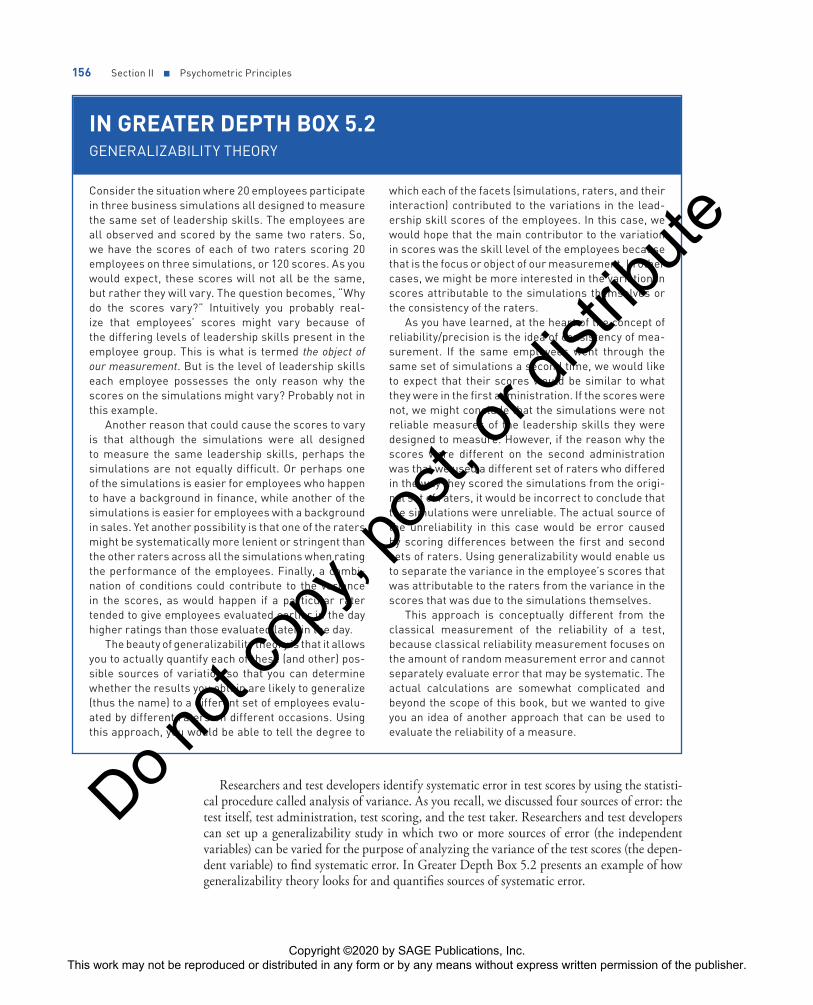
156 Section II ■ Psychometric Principles
IN GREATER DEPTH BOX 5.2GENERALIZABILITY THEORY
Consider the situation where 20 employees participate in three business simulations all designed to measure the same set of leadership skills. The employees are all observed and scored by the same two raters. So, we have the scores of each of two raters scoring 20 employees on three simulations, or 120 scores. As you would expect, these scores will not all be the same, but rather they will vary. The question becomes, “Why do the scores vary?” Intuitively you probably real-ize that employees’ scores might vary because of the differing levels of leadership skills present in the employee group. This is what is termed the object of our measurement. But is the level of leadership skills each employee possesses the only reason why the scores on the simulations might vary? Probably not in this example.
Another reason that could cause the scores to vary is that although the simulations were all designed to measure the same leadership skills, perhaps the simulations are not equally difficult. Or perhaps one of the simulations is easier for employees who happen to have a background in finance, while another of the simulations is easier for employees with a background in sales. Yet another possibility is that one of the raters might be systematically more lenient or stringent than the other raters across all the simulations when rating the performance of the employees. Finally, a combi-nation of conditions could contribute to the variance in the scores, as would happen if a particular rater tended to give employees evaluated earlier in the day higher ratings than those evaluated later in the day.
The beauty of generalizability theory is that it allows you to actually quantify each of these (and other) pos-sible sources of variation so that you can determine whether the results you obtain are likely to generalize (thus the name) to a different set of employees evalu-ated by different raters on different occasions. Using this approach, you would be able to tell the degree to
which each of the facets (simulations, raters, and their interaction) contributed to the variations in the lead-ership skill scores of the employees. In this case, we would hope that the main contributor to the variation in scores was the skill level of the employees because that is the focus or object of our measurement. In other cases, we might be more interested in the variation in scores attributable to the simulations themselves or the consistency of the raters.
As you have learned, at the heart of the concept of reliability/precision is the idea of consistency of mea-surement. If the same employees went through the same set of simulations a second time, we would like to expect that their scores would be similar to what they were in the first administration. If the scores were not, we might conclude that the simulations were not reliable measures of the leadership skills they were designed to measure. However, if the reason why the scores were different on the second administration was that we used a different set of raters who differed in the way they scored the simulations from the origi-nal set of raters, it would be incorrect to conclude that the simulations were unreliable. The actual source of the unreliability in this case would be error caused by scoring differences between the first and second sets of raters. Using generalizability would enable us to separate the variance in the employee’s scores that was attributable to the raters from the variance in the scores that was due to the simulations themselves.
This approach is conceptually different from the classical measurement of the reliability of a test, because classical reliability measurement focuses on the amount of random measurement error and cannot separately evaluate error that may be systematic. The actual calculations are somewhat complicated and beyond the scope of this book, but we wanted to give you an idea of another approach that can be used to evaluate the reliability of a measure.
Researchers and test developers identify systematic error in test scores by using the statisti-cal procedure called analysis of variance. As you recall, we discussed four sources of error: the test itself, test administration, test scoring, and the test taker. Researchers and test developers can set up a generalizability study in which two or more sources of error (the independent variables) can be varied for the purpose of analyzing the variance of the test scores (the depen-dent variable) to find systematic error. In Greater Depth Box 5.2 presents an example of how generalizability theory looks for and quantifies sources of systematic error.
Copyright ©2020 by SAGE Publications, Inc. This work may not be reproduced or distributed in any form or by any means without express written permission of the publisher.
Do not
copy
, pos
t, or d
istrib
ute

Chapter 5 ■ What Is Test Reliability/Precision? 157
Chapter Summary
Psychological tests are measurement instruments. An important attribute of a measurement instrument is its reliability/precision or consistency. We need evidence that the test yields the same score each time a person takes the test unless the test taker has actually changed. When we know a test is reliable, we can conclude that changes in a person’s score really are due to changes in that person. Also, we can compare the scores of two or more people on a reliable test.
No measurement instrument is perfectly reliable or consistent. We express this idea by saying that each observed test score (X) contains two parts: a true score (T) and error (E). Two types of error appear in test scores: random error and systematic error. The more random error present in a set of test scores, the lower the reliability coefficient will be. Another way of saying the same thing is that the higher the proportion of true score variance is of the observed scores, the higher the reliability coefficient will be. Test develop-ers use three methods for checking reliability. Each takes into account various conditions that could pro-duce differences in test scores. Using the test–retest method, a test developer gives the same test to the same group of test takers on two different occasions. The scores from the first and second administrations are then correlated to obtain the reliability coefficient. The greatest danger in using the test–retest method of estimating reliability/precision is that the test tak-ers will score differently (usually higher) on the test because of practice effects. To overcome practice effects and differences in individuals and the test administration from one time to the next, psycholo-gists often give two forms of the same test—alike in every way—to the same people at the same time. This method is called alternate or if certain statistical assumptions are met, parallel forms.
If a test taker can take the test only once, researchers divide the test into halves and correlate the scores on the first half with the scores on the second half. This method, called split-half reliability, includes using the Spearman–Brown formula to adjust the correla-tion coefficient for test length. A more precise way to
measure internal consistency is to compare individu-als’ scores on all possible ways of splitting the test into halves. The KR-20 and coefficient alpha formulas allow researchers to estimate the reliability of the test scores by correlating the answer to each test question with the answers to all of the other test questions.
The reliability of scoring is also important. Tests that require the scorer to make judgments about the test takers’ answers and tests that require the scorer to observe the test takers’ behavior may have error con-tributed by the scorer. We estimate scorer reliability by having two or more persons score the same test and then correlating their scores to see whether their judgments are consistent or have a single person score two occasions of the same test.
To quantify a test’s reliability/precision estimate, we use a reliability coefficient, which is another name for the correlation coefficient when it estimates reliabil-ity/precision. This statistic quantifies the estimated relationship between two forms of the test. The sta-tistical procedure we use most often to calculate the reliability coefficient is the Pearson product–moment correlation. All statistical software programs and many spreadsheet programs will calculate the Pearson product–moment correlation. Coefficient alpha and KR-20, both of which also use correlation, are available in statistical packages only.
To interpret the meaning of the reliability coefficient, we look at its sign and the number itself. Reliability coefficients range from –0.00 (a completely unreliable test) to +1.00 (a perfectly reliable test). Psychologists have not set a fixed value at which reliability can be interpreted as satisfactory or unsatisfactory.
Psychologists use the standard error of measure-ment (SEM) as an index of the amount of inconsistency or error expected in an individual’s test score. We can then use the SEM to construct a confidence interval—a range of scores that most likely includes the true score. Confidence intervals provide information about whether individuals’ observed test scores are sta-tistically different from each other. Six factors—test
(Continued)
Copyright ©2020 by SAGE Publications, Inc. This work may not be reproduced or distributed in any form or by any means without express written permission of the publisher.
Do not
copy
, pos
t, or d
istrib
ute

158 Section II ■ Psychometric Principles
length, homogeneity of questions, the test–retest interval, test administration, scoring, and cooperation of test takers—are important factors that influence the reliability of the test scores.
Another approach to estimating reliability is gen-eralizability theory, which concerns how well and under what conditions we can generalize an esti-mation of reliability from one test to another or on
the same test given under different circumstances. Generalizability theory seeks to identify sources of systematic error that classical test theory would simply label as random error. Using analysis of vari-ance, researchers and test developers can identify systematic error and then take measures to elimi-nate it, thereby increasing the overall reliability of the test.
Engaging in the Learning Process
Learning is the process of gaining knowledge and skills through schooling or studying. Although you can learn by reading the chapter material, attending class, and engaging in discussion with your instruc-tor, more actively engaging in the learning process may help you better learn and retain chapter infor-mation. To help you actively engage in the learning
process, we encourage you to access our new supple-mentary student workbook. The workbook contains critical thinking activities to help you understand and apply information and help you make progress toward learning and retaining material. If you do not have a copy of the workbook, you can purchase a copy through sagepub.com.
Key Concepts
After completing your study of this chapter, you should be able to define each of the following terms. These terms are bolded in the text of this chapter and defined in the Glossary.
alternate forms Cohen’s kappa confidence interval correlation generalizability theory heterogeneous test homogeneous testinternal consistency interrater agreement interscorer agreement
intrarater agreement intrascorer reliability measurement error order effects parallel forms practice effects random error reliability coefficient reliability/precision reliable test
scorer reliability Spearman–Brown formula split-half method standard error of
measurement (SEM) systematic error test–retest method true score
(Continued)
Copyright ©2020 by SAGE Publications, Inc. This work may not be reproduced or distributed in any form or by any means without express written permission of the publisher.
Do not
copy
, pos
t, or d
istrib
ute

Chapter 5 ■ What Is Test Reliability/Precision? 159
Critical Thinking Questions
The following are some critical thinking questions to support the learning objectives for this chapter.
Learning Objectives Critical Thinking Questions
Define reliability/precision, and describe three methods for estimating the reliability/precision of a psychological test and its scores.
•• What are some practical issues that require us to have more than one way to estimate the reliability/precision of a test?
•• Can you think of some common examples where scorer reliability is an important issue that is not related to formally taking a written test, such as scoring in certain Olympic events?
•• If you were told only that the reliability of a test was evaluated by the test–retest method, what questions would you want to ask before concluding that the test was sufficiently reliable/precise?
Describe how an observed test score is made up of the true score and random error, and describe the difference between random error and systematic error.
•• Why is it important to understand the concept of “true scores” even though we can never really know what any person’s true score on a test is?
•• How is the concept of error in a test score different from the everyday concept of error, which is about making a mistake? In what way might the two concepts actually be similar?
Calculate and interpret a reliability coefficient, including adjusting a reliability coefficient obtained using the split-half method.
•• Why is the reliability/precision of a test sometimes referred to as the correlation of a test with itself?
•• If your professor gave a midterm test consisting of only one item, what would you tell him or her about how that might pose a problem for acceptable test reliability?
•• What are some of the questions you would ask if someone told you that the reliability coefficient of a test was negative?
Differentiate between the KR-20 and coefficient alpha formulas, and understand how they are used to estimate internal consistency.
•• Why might calculating coefficient alpha for a test give you a similar result to dividing a test into two parts to estimate reliability?
•• What might it mean if you computed both KR20 and test-retest reliability and found that KR-20 was quite low, but test-retest reliability was much higher?
Calculate the standard error of measurement, and use it to construct a confidence interval around an observed score.
•• Imagine your score on the honors program admissions test was 89 and Jane’s score on the same test was 90. Assume the passing score for admission was set at 90, so Jane was admitted to the honors program while you weren’t. What information would you want to know about the test to understand whether the decision was justified?
•• Why could it be a problem if two people had different scores on a test but the confidence intervals around both scores overlapped?
•• What difficulties might a professor face when calculating a reliability coefficient on a classroom test? Should the test be still be given if the reliability coefficient is not known?
(Continued)
Copyright ©2020 by SAGE Publications, Inc. This work may not be reproduced or distributed in any form or by any means without express written permission of the publisher.
Do not
copy
, pos
t, or d
istrib
ute
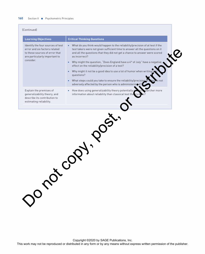
160 Section II ■ Psychometric Principles
Learning Objectives Critical Thinking Questions
Identify the four sources of test error and six factors related to these sources of error that are particularly important to consider.
•• What do you think would happen to the reliability/precision of at test if the test takers were not given sufficient time to answer all the questions on it and all the questions that they did not get a chance to answer were scored as incorrect?
•• Why might the question, “Does England have a 4th of July” have a negative effect on the reliability/precision of a test?
•• Why might it not be a good idea to use a lot of humor when writing test questions?
•• What steps could you take to ensure the reliability/precision of a test is not adversely affected by the person who is administering it?
Explain the premises of generalizability theory, and describe its contribution to estimating reliability.
•• How does using generalizability theory potentially give a researcher more information about reliability than classical test theory does?
(Continued)
Copyright ©2020 by SAGE Publications, Inc. This work may not be reproduced or distributed in any form or by any means without express written permission of the publisher.
Do not
copy
, pos
t, or d
istrib
ute