wesleyan economic working papersrepec.wesleyan.edu/pdf/mimai/2009001_imai.pdf · 1 this version:...
TRANSCRIPT

Wesleyan Economic Working Papers
http://repec.wesleyan.edu/
No: 2009-001
Department of Economics
Public Affairs Center 238 Church Street
Middletown, CT 06459-007
Tel: (860) 685-2340 Fax: (860) 685-2301
http://www.wesleyan.edu/econ
Transmission of Liquidity Shock to Bank Credit: Evidence from the Deposit Insurance Reform in Japan
Masami Imai and Seitaro Takarabe
May 2009

1
This version: May 11, 2009
Transmission of Liquidity Shock to Bank Credit: Evidence from the Deposit Insurance Reform in Japan*
Masami Imai Wesleyan University
Seitaro Takarabe
Wesleyan University JEL Codes: E44, G21
Key Words: Deposit Insurance, Bank Lending Channel, Japan, Natural Experiment
* We would like to thank Eugene Baek, John Bonin, and Richard Grossman for valuable comments.
All errors are ours.
Corresponding author: Masami Imai, Department of Economics, Wesleyan University, Middletown,
CT 06459-0007. Tel: 860-685-2155, Fax: 860-685-2301.

2
Transmission of Liquidity Shock to Bank Credit: Evidence from the Deposit Insurance Reform in Japan
Abstract
Finding the causal effects of liquidity shocks on credit supply is complicated by the
endogenous relation between loan demand and liquidity position of banks. This paper
attempts to overcome this problem by exploiting, as a natural experiment, the
exogenous deposit outflow prompted by the removal of a blanket deposit guarantee
on time deposits in Japan. We find that just as the government placed a cap on
insurance for time deposits in 2002, weak banks suffered from a large outflow of
partially insured time deposits. More importantly, we find that those weak banks were
not able to raise a sufficient amount of fully insured ordinary deposits to make up for
the loss of time deposits, which, consequently, forced them to cut back on loan supply.
These results are consistent with the theory that the imperfect substitutability of
insured deposits and uninsured deposits affects the tightness of banks’ financing
constraints and ultimately the supply of bank loans.
JEL Codes: E44, G21
Key Words: Deposit Insurance, Bank Lending Channel, Japan, Natural Experiment

3
1. Introduction
The question of how exactly liquidity shocks in a banking sector are transmitted to
the real economy has long been a subject of active discussion in the field of both
finance and macroeconomics. On the one hand, according to the Modigliani-Miller
Theorem, even when exposed to periodic negative liquidity shocks, banks should be
able to raise sufficient funds from alternative sources swiftly to make up for the
temporary funding shortfall and thus be able to finance all profitable lending
opportunities (Modigliani and Miller, 1958). On the other hand, in the presence of
informational asymmetry on the value of bank assets (i.e., banks know more about the
quality of their own assets than outside investors do), banks will face a lemon
premium on external funds, which means that negative liquidity shocks would raise
overall funding costs, thereby forcing banks to cut back on loan supply to non-
financial sectors (Bernanke and Blinder, 1992; Stein 1998).1
The empirical work on the relationship between liquidity and bank lending
has explored how bank lending responds to liquidity shocks in aggregate data
(Bernanke and Blinder, 1992; Kashyap, Stein and Wilcox, 1993; Bernanke and
Gertler, 1995). More recently, the empiricists have moved away from the use of
aggregate data and have begun to use disaggregated bank-level data. The motivation
for such a shift in the empirical focus is that the analysis of aggregate data suffers
1 This type of information asymmetry also induces banks with high quality assets to hold an excessive
amount of risk-free securities so as to avoid having to pay lemon adverse selection premium for
external funds (Lucas and MacDonald, 1992).

4
from a serious identification problem (i.e., liquidity shocks are likely to coincide with
shifts in a loan demand schedule).
Furthermore, the use of bank-level data reveals the exact mechanism of the
bank lending channel: the effects of liquidity shocks on loan supply are much larger
for smaller, less liquid, and less well-capitalized banks since the funding
opportunities of these banks depend critically on the severity of an adverse selection
problem (Kashyap and Stein, 2000; Kishan and Opiela, 2000; Jayaratne and Morgan,
2000).
However, even these recent empirical works potentially suffer from a subtle
identification problem -- the lending opportunities of banks might not be completely
orthogonal to their balance sheet characteristics and/or their deposit flows. For
example, a flow of deposits into banks is not entirely exogenous. Banks with more or
better lending opportunities might be willing to pay higher interest rates and attract
more deposits so as to finance those lending opportunities. The low level of
capitalization or liquidity is not entirely exogenous either. It is likely to be a symptom
of a worsening economic environment that a particular bank is, or has been, facing;
i.e., more often than not, banks become poorly capitalized and illiquid as they suffer
from a large amount of financial losses on their investments.2
This paper examines the transmission of liquidity shocks to loan supply in
Japan’s banking sector. The main innovation of this paper is credible econometric
2 It is also possible that the results might suffer from the bias in the opposite direction if weak banks
pursue “gambling for resurrection” strategy by aggressively expanding deposits and risky loans (e.g.,
Brumbaugh and Carron, 1987; Kane, 1989; Barth 1991) although literature on the banking lending
channel has not focused on this issue.

5
identification of liquidity shocks by exploiting the removal of a blanket deposit
guarantee in Japan as a natural experiment. When the Japanese government lifted a
blanket guarantee and imposed a limit on time deposits, Japan’s banking system
experienced a clear regime shift. In the old regime, depositors did not face the risk of
putting their deposits into “lemon” banks, which in theory must have allowed banks
to avoid adverse selection problems all together when raising external funds. In the
new regime, the ability of banks, especially weak ones, to raise partially insured time
deposits was severely undermined because depositors had incentives to ration funds
to risky banks in order to protect themselves from financial losses.
This quasi-experiment is relatively clean because the change in the deposit
insurance scheme was not driven by deterioration or improvement in banks’ business
environment. Rather, the lifting of a blanket guarantee was scheduled ahead of time
so that the timing of the shocks was likely to be orthogonal to the demand condition
of the banking sector.
We find four notable results. First, we find that banks seem to have been
unconstrained during the period of a blanket guarantee: weak banks and strong ones
expanded their deposits at a similar rate, and loan and deposit growth were
uncorrelated. Second, we find that as the government placed a cap on deposit
insurance in 2002, weak banks lost a large amount of partially insured time deposits
as found in Imai (2006), Murata and Hori (2006), and Fueda and Konishi (2007).
Third, we find that these weak banks were not able to raise a sufficient amount of
other types of deposits to replace the loss of time deposits; that is, their total deposits
declined along with time deposits which were directly affected by the deposit

6
insurance reform. Fourth and last, bank deposit growth, when instrumented with bank
financial strength, had statistically significant and economically important effects on
loan growth during the period of transition from a blanket guarantee to a limited
guarantee. These results highlight the role of imperfect substitutability of insured and
uninsured deposits in the transmission of liquidity shocks to bank lending.
The present paper is also relevant to a large body of literature on the bank
lending channel in Japan (e.g., Ogawa and Kitasaka, 2000; Ito and Sasaki, 2002; Woo,
2003; Taketa and Udell, 2007). The methodology of this paper is similar in spirit to
more recent papers (Peek and Rosengren, 2000; Gan, 2007; Watanabe, 2007) that
make an attempt to pursue more credible identification of financial shocks on the
capital position of banks.3 Our results are largely consistent with the commonly-held
notion that the presence of problem banks led to a reduction in the flow of
intermediated funds and exacerbated the recession in Japan.
This paper is also closely related to two recent papers (Khwaja and Mian,
2008; Paravisini, 2008) in terms of its methodology. Khwaja and Mian (2008) make
use of the announcement of a nuclear test by the Pakistani government which
precipitated a rapid outflow of foreign currency deposits from the Pakistani banks in
order to cleanly identify a deposit shock. Paravisini (2008) uses the exogenous
infusion of cash from the government to banks in Argentina to study the transmission
of liquidity shocks to loan supply. The common key element that allows clean
3 Peek and Rosengren (2000) use the Japanese stock market and real estate problems in the early 1990s
to identify loan supply shocks to U.S. commercial real estate markets. Gan (2007) and Watanabe
(2007) utilize the collapse of asset values in the early 1990s in Japan and banks’ real estate exposure to
instrument financial shocks to Japanese banks.

7
identification of liquidity shocks in both these papers and our paper is that the
external shock is likely to be unrelated to loan demand and it has differential effects
on the liquidity position of different banks.
The remainder of this paper is organized as follows: Section 2 briefly
describes the background of Japan’s financial system and the nature of the deposit
insurance reform. Section 3 discusses our data and empirical strategy. Section 4
presents the results, followed by robustness checks in Section 5. Section 6 concludes
with possible direction of future research.
1. Japan’s Financial System
A. Corporate Reliance on Bank Borrowing
Banks have played an essential role in the financial system and have been a
dominant source of external finance for business firms in post-war Japan. Until the
mid-1980s, the ratio of bank borrowing to total corporate finance was steady at over
80 percent. Most of the remainder funds were raised by new equity issuance (Hoshi
and Kashyap, 2001).4 In the mid-1980s, the government deregulated restrictions on
the issuing of corporate bonds and motivated firms to shift their finance to domestic
and foreign bond financing. Bank borrowing, however, still constituted around 75
percent of the total corporate finance by 1995 and remained a principal means of
financing for most of the firms.
4 As it is consistent with a view that banks (partially) solves asymmetric information problem in credit
market by monitoring and maintaining relationships with firms (Sharpe, 1990; Rajan, 1992; Diamond,
1984, 1991), Japanese firms that had a close tie with banks were found to be less liquidity constrained
than those without strong bank ties (Hoshi, at al. 1990, 1991).

8
While large, reputable firms gained better access to open markets to raise
external funds as a result of financial deregulation, small and medium-sized domestic
firms continued to rely on bank financing (Hoshi and Kashyap, 2001). The fraction of
small and medium-sized business loans to total loans that was 73 percent over the
period 1977 to 1986 increased to 78 percent over the period 1987 to 1990 (Ogawa
and Kitasaka, 2000)5. Hence, Japan’s economy as a whole continued to be highly
dependent on bank financing and banks seem to have played a central role in the
economy even after financial deregulation.
B. Evolution of Deposit Insurance System in Japan
Following the financial turmoil and a number of bank failures in the 1990s,
the government announced in 1995 that it would provide a blanket guarantee on all
bank deposits from June 1996 to March 2001 under the objective of avoiding a
potential systemic banking crisis.6 Thus, the depositors never faced the real risk of
losing their deposits during this time period.
5 The corporate reliance on bank borrowing was especially prevalent for small and medium-sized firms
in the service, construction and real estate industries (Dekle and Kletzer, 2003).
6 As in other countries the Japanese government gradually expanded deposit insurance coverage over
time since it was first instituted up to one million yen in 1971. The government raised its cap to three
million yen in 1972, and ten million yen in 1986. In addition to the formal explicit deposit insurance,
the Japanese government implicitly guaranteed bank deposits traditionally in the form of the convoy
system, in which the Ministry of Finance (MOF) encouraged a healthy bank to rescue a failed bank by
providing both personnel and financial assistance using the reserves of Deposit Insurance Corporation
(Hoshi, 2002).

9
The blanket guarantee, when it was first introduced, had an expiration date --
it was scheduled to be removed in March 2001. The Japanese government, however,
expressed concern that the end of full guarantees might cause the rapid outflow of
deposits and severely hurt small and medium-sized financial institutions.7
Consequently, in December 1999, the government decided to postpone the re-
introduction of the insurance cap for time deposits by one year and by two years for
ordinary deposits. In April 2002, the deposit insurance cap of ten million yen was
placed on time deposits as promised. However, due to the continuing instability of the
financial system, in October 2002 the government again postponed complete
implementation of the insurance cap on all the other deposits until April 2005.8
Since the time deposits were no longer fully insured after April 1st of 2002,
depositors quickly shifted their deposits from time deposit accounts to ordinary
deposit accounts during the transition period of 2001-2002. Figure 1 illustrates the
dramatic shift of the deposit composition. Figure 2 highlights the massive outflow of
large time deposits (over ten million yen) before 2002, suggesting that the reform had
disproportionately larger effects on large time deposits than small time deposits since
time deposits less than ten million yen would not be exposed to any risk by the reform.
In addition to the substantial substitution from time deposits to ordinary deposits,
7 Michio Ochi, chairman of the cabinet-level Financial Reconstruction Commission, expressed a
concern that, “if 10% of credit cooperatives collapse, there will be an exodus of funds out of the entire
credit cooperative industry. Such a development would rekindle anxiety toward not only those
particularly small financial institutions but also the nation's financial industry as a whole.” December
23, 1999. Japan Economic Newswire.
8 See more details in Fukao (2007).

10
some studies show that the reform also prompted depositors to reallocate their
deposits from risky banks to financially healthy banks (Imai, 2006; Murata and Hori,
2006; Fueda and Konishi, 2007).
Figure 1 and 2 also show that, time deposits began to decline gradually a year
before the reinstatement of the insurance cap in April 2002. Since the deposit
insurance reform was already announced, it is reasonable to infer that some
depositors were anticipating the reinstatement and reallocated their large time
deposits ahead of time. Moreover, earlier studies on the reform (Imai, 2006; Murata
and Hori, 2006; Fueda and Konishi, 2007) show that most of the depositors reacted to
the reform during the period of transition.
C. The Credit Crunch in 2002
Many economists argue that the credit crunch which followed the collapse of
asset prices caused or exacerbated the long economic stagnation, so-called “Lost
Decade” or “Great Recession” (Kuttner and Posen, 2001; Hoshi and Kashyap, 2004;
Fukao, 2007). Figure 3 illustrates the fluctuation of lending attitude of financial
institutions in Japan from The BOJ Tankan.9 It shows two severe credit crunches in
1991 and 1998.
9 The BOJ Tankan is compiled by the Bank of Japan based on its quarterly survey about the present
and future business conditions for Japanese business firms. It is considered to be one of the most
important economic indicators with which the Bank of Japan conducts its monetary policy. See
Motonishi and Yoshikawa (1999) and the relevant website in BOJ
(http://www.boj.or.jp/en/theme/research/stat/tk/index.htm) for more details.

11
The first credit crunch followed the collapse of the bubble economy; the sharp
decline in asset prices drastically undermined the value of wealth and collateral and
led the economy to a severe recession. The second credit crunch occurred after a
number of bank failures including the failure of Hokkaido Takushoku Bank, a large
nation-wide bank, and Yamaichi Securities, one of the Japan’s oldest and largest
brokerage firms. These credit crunches have been studied extensively and reported to
have had a significant adverse impact on financing costs and real economic activities
(Motonishi and Yoshikawa, 1999; Peek and Resengren, 2001).
In addition to these two credit crunches, Figure 3 also displays an additional
credit crunch in 2002. Figure 4 gives a closer look at the change in the lending
attitude of financial institutions from 2001 to 2003. It shows that the lending attitude
worsened sharply in the first quarter of 2002 and remained relatively low in the
subsequent periods. The common explanation for this credit crunch is the collapse of
the IT bubble in the 2000.10 NASDAQ Composite peaked in March 2000 and sharply
dropped down to one third of its peak in April 2001. As Figure 5 shows, Nikkei 225
Index also followed a similar path with NASDAQ Composite and consistently
declined until late 2002.
However, while the collapse of the IT bubble might have been the culprit for
the 2002 credit crunch, the timing of the credit crunch does not correspond perfectly
10 For example, “waves from the U.S. high-tech and economic slump continue to crash onto Asian
shores: Analysts fear the onset of a global recession and Japanese tech giant Fujitsu said Monday that
it will cut 16,400 workers. The U.S. economy - especially the technology sector - was the primary
locomotive for the export economies of Japan, Korea, Taiwan and Malaysia. Now that the bubble has
burst here, it's having a devastating effect on Asia.” August 21st, 2001. USA TODAY.

12
to the fall in the stock markets. Despite the sharp decline in stock markets in 2000, the
lending attitude of Japanese banks remained strong and even improved slightly.
Instead, the lending attitudes declined sharply much later in the first quarter of 2002,
which coincided with the removal of a blanket deposit guarantee. According to these
observations, one can speculate that the reform-induced deposit shock may have
quickly led to the deterioration in the lending attitude of financial institutions in the
first quarter of 2002, although it is difficult to make a definite conclusion based on the
movement of the aggregate variable in response to a one-time shock.
2. Data and Empirical Strategy
A. Measurement of Bank Financial Strength
We choose to use the Moody’s ratings because of well-known unreliability of
balance sheet items during this particular period in Japan (e.g., Genay, 2002, Fukao,
2002).11 While certainly not perfect, it has been shown that Moody’s ratings are
11 As the Japanese government failed to enforce rigorous prudential regulation, the accounting
measures of bank risk were frequently manipulated by Japanese banks and subsequently began to lose
its explanatory power for bank’ share prices (Genay, 2002). For instance, banks issued subordinated
loans to the group-affiliated life insurance companies in exchange for holding subordinated loans and
surplus notes of those life insurance companies and they gained quasi capital on their balance sheet
through this “double-gearing” (Fukao, 2002). Not surprisingly, when we use the accounting measures
of bank risk, we do not find any meaningful results, indicating a serious measurement error. The
results of these specifications are not reported in this paper to conserve space, but are available from
the authors upon request.

13
relatively more reliable for evaluating performance of Japanese banks (Bremer and
Pettway, 2002; Li, Shin, and Moore, 2006).
The rating used here is Moody’s Long-Term Bank Deposit Ratings (MBDR),
which measure a bank’s ability to repay punctually its foreign and/or domestic
currency deposit obligations. I assign numerical values to each rating in the ascending
order: MBDR = 1 for “Aa3”; MBDR = 2 for “A1”; MBDR = 3 for “A2”; MBDR = 4
for “A3”; MBDR = 5 for “Baa1”; MBDR = 6 for “Baa2”; MBDR = 7 for “Baa3”;
MBDR = 8 for “Ba1”. The assigned number reflects degree of bank risk (i.e., the
riskier the bank, the higher the MBDR).
B. Loans and Deposits
The main variables of our interest are loans and deposits. Those financial
variables including total, time, and ordinary deposit and total loan are drawn from
Nikkin Shiryo Nenpo (Annual Report on Japan’s Financial Institutions) published by
the Japan Financial News. Loan and deposit variables are calculated into annual
growth.12
C. Empirical Strategy
We expect a bank’s liquidity constraints to be tight only when depositors face
the significant possibility of default under the partial guarantee and are concerned
about the risk of picking “lemon” banks. Thus, there is no compelling reason to
12 See Tables A1 and A2 in Appendix A for the complete list of data descriptions, sources and
summary statistics.

14
expect deposits at weak banks to grow slower than those at strong banks during the
period of full guarantees. On the other hand, we expect that under the partial
guarantee, weak banks will suffer from an outflow of uninsured deposits. As a result,
if uninsured and insured deposits are not perfect substitutes, their total deposits will
fall, which, in turn, translates into the leftward shift of the loan supply schedule.
To implement this empirical strategy, we relate bank deposits to banks’ risk
profiles in the first stage regression. In the second stage, we explore how a deposit
shock affects loan supply. We identify deposit shocks by an instrumental variable
approach. Since the reform made deposits sensitive to bank default risk and the
deposit supply was reallocated largely based on bank financial strength, we can use
the bank financial strength as an instrument to purge the endogenenous components
of deposits that are correlated with loan demand.
Hence, we first examine a simple statistical relationship between the growth
of various types of deposits and bank financial strength:
0 1i i iDeposit MBDR (1)
∆Deposit is growth of time, ordinary or total deposit. MBDR is Moody’s Bank
Deposit Ratings at the beginning of fiscal year. A subscript i indicates the bank.
Using cross-sectional bank-level data, we estimate the equation for 2001-2002, the
transition period when the reform provided depositors with the incentive to reallocate
their funds across different types of deposit accounts and different banks. Therefore,
we expect MBDR to be negatively correlated with partially insured time deposits.
However, in the equation for ordinary deposit, we expect the coefficient on MBDR to

15
be positive since risky banks should attempt to make up for the shortfall of time
deposits by issuing more ordinary deposits which were still fully insured unlike time
deposits.
If insured deposits are perfect substitute for uninsured deposits, then weak
banks would be able to raise a sufficient amount of funds from other types of deposits
to fully compensate for the loss of time deposits and, consequently, total deposits
should remain the same. Under this scenario, the coefficient on MBDR in the equation
for total deposits will be small and statistically insignificant. If, on the other hand,
insured and uninsured deposits are not perfect substitutes, then weak banks would
face increasing marginal costs as they attempt to raise additional funds, which, in turn,
forces banks to cut bank on loan supply. Under this scenario, the coefficient on
MBDR in the equation for total deposits will be negative, just like in the equation for
time deposits.
We also estimate the same equation for 2000-2001, the period of a full deposit
guarantee, as a falsification exercise. During this period, given that all deposits were
fully guaranteed, there is no reason to expect MBDR to have had any effects on the
supply of deposits. If deposit growth turns out to be negative correlated with MBDR
even during 2000-2001, we would have to suspect that there might have been
systematic relation among loan demand, deposit demand, and MBDR.
In the second stage, we relate loan growth to deposit growth while
instrumenting the latter with MBDR:
0 1i i iLoan Deposit (2)

16
∆Loan is total loan growth and iDeposit is the predicted value of the deposit growth
from the first stage regression.13 We use Limited Information Maximum Likelihood
(LIML) method as it is shown to be more robust to weak instrument problems,
compared to Two Stage Least Squares (TSLS) (Stock and Yogo, 2002). If banks are
liquidity-constrained, loan supply should be positively correlated with the change in
deposit; that is, the coefficient on iDeposit should be positive.
3. Baseline Results
Table 1 reports the estimation results of simple OLS regressions of loan
growth on deposit growth for 2001-2002 and 2000-2001 in columns 1-4 and the
results of the IV regression (Equations (1) and (2)) for 2001-2002 and 2000-2001 in
columns 5-10. Panels A and B report the results of the first stage and second stage
equations, respectively. The third row gives dependent variables that are estimated for.
TIME, ORDI, TOTAL, and LOAN represent growth of time deposits, ordinary
13 In this specification, we relate the loan growth during 2001-2002 to a contemporaneous deposit
shock that is caused by the reform; that is, we assume that bank loan responds rather quickly to deposit
shocks. It might be reasonable to question this assumption: it might take bank loans much longer to
respond to deposit shocks. We try relating the 2002-2003 loan growth to the 2001-2002 deposit shocks
but we do not find any meaningful results (the results are available from the author upon request),
suggesting that bank lending responds to deposit shocks relatively quickly. The quick response of loan
supply to deposit shocks is documented in other papers as well. Paravisini (2008) finds that financial
shocks to constrained banks in Argentina have an immediate effect on loan supply and the lending
response occurs within a quarter from the shock. Khwaja and Mian (2008) also find that loan supply
shifts swiftly in response to liquidity shocks in their study of Pakistani banks.

17
deposits, total deposits and total loans, respectively. The coefficients on MBDR
capture sensitivity of the deposit growth to bank default risk.
In OLS, the coefficient on Time Deposit Growth turns out positive and
statistically significant for loan growth for the transition period in 2001-2002 (column
1) whereas loan growth was uncorrelated with deposit growth during 2000-2001
(columns 3-4). These results are consistent with the view that the availability of time
deposits was indeed a major determinant of loan supply during 2001-2002 while it
was not a constraint for banks to expand loans during the period of the blanket
guarantee. Although the deposit growth in these regression equations is endogenous
(and the results should be interpreted with caution), these pieces of evidence seem to
confirm the view that the nature of the deposit insurance scheme is related to the
tightness of liquidity constraints in the banking sector.
The IV results also show a strong negative correlation between bank default
risk (MBDR) and time deposit flows in the post-reform period (column 5, Panel A),
indicating that depositors became sensitive to bank default risk in the selection of
banks and withdrew more time deposits from those poorly rated (or financially weak)
banks.
The coefficient on MBDR is positive but not statistically significant in the
equation for ordinary deposit (column 6, Panel A). These results are in accordance
with the fact that the reinstatement of the insurance cap was placed only on time
deposits. Since the ordinary deposit was still fully insured, depositors switched their
time deposit accounts to ordinary deposit accounts. If all the depositors just switched
their time deposit account to an ordinary deposit account within the same bank, we

18
should observe a statistically significant rise in ordinary deposits absorbing all the
losses of time deposits. The fact that the coefficient is positive but not statistically
significant, however, implies that some depositors might not have simply switched
the accounts but moved away from financially weak banks to strong ones or to other
financial tools.
These results on ordinary deposits also confirm that the observed decline in
time deposits was not driven by a decline in loan demand; i.e., if the leftward shifts in
loan demand schedule had been the culprit, ordinary deposits at weak banks would
have declined along with time deposits.
Column 7 in Panel A shows that MBDR is negative and statistically significant
for the growth of total deposits, which also suggests that financially weak banks could
not fully replace the loss of time deposits with other deposits. This implies that time
deposits and other deposits are not perfect substitutes.14
In contrast to the results for the period 2001-2002, bank default risk did not
have any significant effects on deposit flows in the pre-reform period (columns 8-10,
Panel A). Before the implementation of the insurance cap, depositors had no incentive
14 These results also highlight the violation of the Modigliani-Miller theorem. Modigliani-Miller
theorem states that, in the absence of taxes, bankruptcy costs and asymmetric information, firms have
perfect substitutability between any financing methods and that market will supply the funds for all
projects that yield an expected positive net present value (Miller and Modigliani, 1958). Thus, if the
assumptions of Modigliani and Miller theory hold, total funding growth should be unaffected by the
availability of time deposits. The empirical fact that the total deposit growth was affected by financial
weakness and the shift in the availability of time deposits suggests that financial markets are not
perfect.

19
to actively select financially strong banks, and therefore, banks’ financial strength
was irrelevant to deposit flows under the full deposit guarantee. Those extremely low
R-squared and F-Statistic also underscore that bank default risk is uncorrelated with
the deposit flow. These results also serve as placebo tests. If MBDR is spuriously
correlated, in a systematic fashion, with lending opportunities and thus demand for
external funds across individual banks, MBDR should have a statistically significant
coefficient even during the 2000-2001; i.e., in order to finance their good lending
opportunities, highly rated banks should aggressively pursue deposits. The results
suggest that such phenomena did not occur in 2000-2001, which indicates that MBDR
is likely to be a valid instrument which is strongly correlated with the deposit growth
but uncorrelated with the lending opportunities of individual banks in 2001-2002.
Finally, even when instrumented with MBDR, the coefficient on Time Deposit
Growth is positive and statistically significant (column 5, Panel B), meaning that
poorly rated banks reduced loan supply in response the outflow of time deposits. The
positive and statistically significant coefficient on Total Deposit Growth (column 7,
Panel B) also indicates that there is a strong correlation between loan growth and the
exogenous component of total deposit growth. 15 In particular, this coefficient is
approximately equal to one, suggesting that the magnitude is economically important:
a loss of deposit by 1 percent leads to a contraction of loan supply by 1 percent. In
15 Note, however, that the results on the total deposit growth (column 7) are not as reliable as those on
the time deposit growth, given the results seem to exhibit a weak instrument problem with F-Statistic
of 6.045.

20
sum, these results suggest that banks view insured and uninsured funds as imperfect
substitutes, which makes bank loans more sensitive to funding shocks.
4. Robustness Checks
While our simple framework generates evidence for the presence of the bank
lending channel, it is possible that there might be some missing confounding factors
that we have not accounted for. In particular, isolating shifts in loan supply schedule
from shocks affecting loan demand is always a formidable task in the bank lending
channel literature since the interaction of loan demand and supply determines the
observed loan quantity. The omission of the loan demand factor thus could cause
overestimation bias when estimating loan supply if determinants of loan supply are
allowed to absorb the effects of loan demand on loan quantity. In our case, although
we have established that Moody’s rating was likely to be uncorrelated with loan
demand (and deposit demand) during 2000-2001, we cannot rule out the possibility
that such correlation arose during 2001-2002 for some reasons that are unknown to us.
In this section, we make various attempts to control for heterogeneity across banks.
A. Geographical Differences
Those banks in our sample operate in different parts of Japan and thus face
different demand conditions, depending on the performance of local economies. To
control for heterogeneity in local loan demand, we use four different prefecture-level
variables: land price, GDP, bankruptcy, and job opening ratio. Land price is the
average annual price indices of commercial sites of prefectures and obtained from

21
Japan Statistical Yearbook published by Statistics Bureau, Director-General for
Policy Planning (statistical standards) and Statistical Research and Training Institute
of Ministry of Internal Affairs and Communication. GDP is annual prefecture level
GDP complied by Cabinet Office of the Government of Japan. The number of
bankruptcies is from Teikoku Bank Data. The job opening rate is calculated as the
number of job seekers divided by the number of job openings and drawn from
Ministry of Health, Labor and Welfare. All the variables are calculated into annual
growth.
Since these loan demand controlling variables are at a prefecture-level while
the rest of the variables in the data set are at a bank-level, we construct the branch-
weighted average of each controlling variable for each bank as follows:
,
1_ ( _ * _ )
_i j i jji
BANK DEMAND PREF DEMAND PREF BRANCHTOTAL BRANCH
where BANK_DEMAND is the branch-weighted average of a loan demand variable
for a bank i, TOTAL_BRANCH is the total number of branches of bank i,
PREF_DEMAND is a loan demand variable for prefecture j, and PREF_BRANCH is
the number of branches of bank i in prefecture j. This equation is used to calculate
each loan demand variable separately. For instance, a branch-weighted land price for
bank i is calculated as follows:
,
1_ ( _ * _ )
_i j i jji
BANK LAND PREF LAND PREF BRANCHTOTAL BRANCH

22
where PREF_LAND is the growth rate of the land price index in commercial sites for
prefecture j.
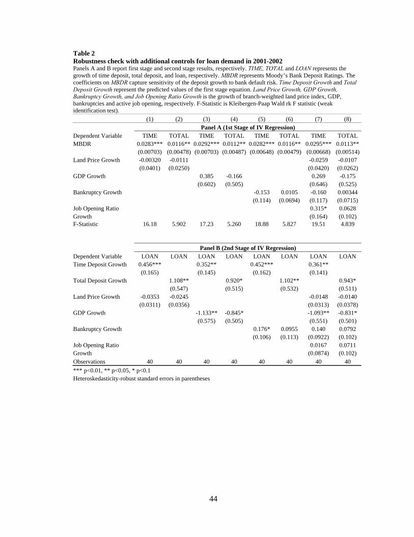
Table 2 displays the results. The coefficients on MBDR remain negative and
statistically significant for both time and total deposit growth in the first stage (Panel
A). Similarly, in the second stage results, the coefficients on Time Deposit Growth
and Total Deposit Growth are positive and statistically significant (Panel B). Hence,
our main results are statistically robust to the inclusion of these additional control
variables. The coefficients on deposits in columns 7-8 in Panel B are slightly smaller
in magnitude compared to the results without any demand controls in Panel B of
Table 1. This aligns with our anticipation that controlling for demand corrects the
overestimation bias that was expected to be present in the results for Equation (2) in
Table 1.
B. Bank Type
Banking literature shows that banks of different sizes serve different types of
borrowers. In particular, large banks tend to serve large borrowers while small banks
tend to serve small opaque borrowers (Berger, Miller, Petersen, and Rajan, 2005).
Thus, if demand condition changes for a particular segment of borrowers in a way
that is correlated with bank size, excluding the size of banks might give misleading
results. Although financial deregulation blurred the difference between small local
banks and large nation-wide banks in Japan, it might still be the case that small local
banks serve mainly small opaque borrowers relative to large banks (Uchida, Udell
and Watanabe, 2008). To address this issue, we include the log of bank assets to

23
capture bank size and dummy variables for trust banks, tier I regional banks, and tier
II regional banks as additional controls.16
Table 3 reports the results of these specifications. Even after including these
controls, the results largely match the previous findings that bank default risk has
negative and significant effects on deposit flows in the first stage (Panel A) and that
the instrumented values of deposit growth are positively correlated with loan growth
in the second stage (Panel B). Bank size turns out to be positive and statistically
significant for total deposit growth (column 2, Panel A) and negative and statistically
significant for loan growth (column 2, Panel B). These results suggest that depositors
reacted to the deposit insurance reform by putting their money into large banks which
happen to have had limited lending opportunities relative to the average bank in our
sample.
Trust and Tier I Regional Banks have a positive and statistically significant
coefficient for time deposit growth (column 3, Panel A). This indicates that those
non-city banks or smaller banks attracted more time deposits or suffered less from the
time deposit outflow holding everything else constant. In the second stage, the
coefficients on regional bank dummies are positive and statistically significant
16 There are four major types of commercial banks in Japan; city bank, Tier I and Tier II regional bank,
and trust bank. City banks are large major commercial banks that base their headquarters in a big city
and have nation-wide operation. Regional banks are small or medium-sized banks that operate in
specific local areas. They are divided into Tier I and Tier II regional banks: Tier I regional banks are
generally larger than Tier II. Trust banks are commercial banks that specialize in being a trustee of
various kinds of trusts and in managing estates. These four types of banks constitute over 80 percent of
the total assets held by all the banks operated in Japan.

24
(column 3, Panel B), suggesting that the lending opportunities of small regional banks
had improved, relative to that of large nationwide banks, during the sample period.
For total deposits, the coefficients on the bank type dummy variables in the first stage
are negative but none of them is statistically significant (column 4, Panel A).
In the second stage, the coefficients on all the dummy variables, however, are
positive and statistically significant (column 4, Panel B), which is consistent with the
earlier result that non-city banks issued more loans on average. When bank size and
dummy variables for bank types are included at the same time, the coefficients on
these variables lose statistical significance in the second stage, suggesting some
collinearity problem (columns 5-6, Panel B).
C. Controlling for Loan Write-Off
Peek and Rosengren (1995) point out that it might be misleading to use the
change in outstanding loans as a measure of the change in the credit availability
because the change in the outstanding loans reflects more than just new loan
origination but also includes charge-offs, transfer of real estate loans to other real
estate owned due to foreclosures, and net loan sales. One might worry that this
criticism is especially applicable to our study because the Japanese banks
accumulated a large number of non-performing loans and might have been compelled
to write off a large number of non-performing loans from their balance sheets.
Moreover, if weak banks had to write off more bad loans than strong ones in a
systematic fashion during the sample period, then MBDR is no longer valid
instrument since it is mechanically correlated with loan growth through differential

25
amounts of loan write-offs. In this robustness check, we add these write-offs back to
the total amount of loans and calculate the loan growth so that the changes in loans
are not attributed to the loan write-offs.
Table 4 reports the results with write-off adjusted loan growth. While the size
of coefficients on the deposit growth decreases slightly compared to the baseline
results (Panel B, Table 1), these results are qualitatively similar. The results also
suggest that, although the amount of write-offs during the sample period was
relatively large, they had no systematic relation to the weakness of banks, leaving our
main results intact.
D. Panel IV Estimation
The last possible confounding factor we consider is time-invariant bank
specific demand conditions; i.e., if unobserved bank specific characteristics that are
correlated with loan demand are also correlated with MBDR, then the results are
biased. To address this issue, we pool the data from 2000 to 2002 and carry out panel
IV estimation with bank fixed effects, which should purge out the effects of
unobserved bank characteristics that are time-invariant.
Table 5 reports the results. REFORM*MBDR is an interaction term of a
dummy variable for 2001-2002 and MBDR. This variable captures sensitivity of the
deposit growth to bank default risk during the period of transition. REFORM*SIZE is
an interaction term of a dummy variable for 2002 and SIZE that is lagged by one.
This captures sensitivity of deposit and loan to SIZE after the reform in 2002.

26
The coefficients on REFORM*MBDR are negative and statistically
significant in the equations for time deposits (columns 1, 3 and 5, Panel A), implying
that the deposit insurance reform made time deposits sensitive to bank default risk.
Furthermore, those coefficients on Time Deposit Growth are positive and also
statistically significant in all the equations (columns 1, 3, and 5, Panel B), suggesting
a positive correlation between instrumented deposit growth (i.e. exogenous deposit
shock) and loan growth. 17 The coefficient on REFORM*SIZE is negative and
statistically significant in both the first and second stage (column 5), suggesting that
larger banks lost more time deposits and made fewer loans during the transition from
the full guarantee to the limited one from 2001-2002. REFORM*SIZE is statistically
significant in neither the first nor second stage (column 6). These results are all in line
with all the previous findings and support our main conclusions.
5. Conclusion
This paper utilizes the exogenous deposit outflow caused by the removal of a
blanket deposit guarantee in Japan to investigate the impact of liquidity constraints on
loan supply in Japan’s banking sector. The empirical results show that as the
government placed a cap of deposit insurance in April 2002, depositors began to
reallocate deposits based on banks’ financial strength and bank deposit became
sensitive to bank default risk. Furthermore, weak banks that experienced a large
outflow of time deposits could not fully make up for the loss with other types of funds
due to imperfect substitutability of insured and uninsured deposit.
17 The results on total deposits seem to exhibit the sign of weak instrument problem (e.g., low first stage F-statistics and large standard errors in the second stage results).

27
More importantly, we find that bank deposit growth, when instrumented with
bank financial strength, had a statistically significant and economically important
impact on loan growth during the period of transition from a blanket to a limited
guarantee. These results suggest that liquidity shocks matter to loan supply precisely
in an environment where the adverse selection problem becomes an issue when
raising uninsured deposits.
While this paper presents strong evidence for the presence of liquidity
constraints in the particular context of Japan’s deposit insurance reform, one may
wonder whether the results can be generalized to other settings. In particular, one can
speculate that these results are likely to depend on the fragility of financial
institutions, informational environments and liquidity of financial systems as a whole.
Similar to the case of Japan, as many as 14 countries have also adopted a temporary
blanket guarantee during the financial crisis and shifted back to a limited guarantee
(Laeven and Valencia, 2008). Hence, a similar experience in deposit insurance regime
in other countries provides a suitable test ground to replicate our results, which should
be a fruitful area for future research.

28
References
Barth J. (1991). The Great Savings and Loan Debacle. Washington D.C.: American
Enterprise Institute.
Berger, A. N. and N. Miller, M. Petersen, R. Rajan and J. Stein (2005). Does
Function Follow Organizational Form? Evidence from the Lending Practices
of Large and Small Banks. Journal of Financial Economics 76(2): 237-69.
Bernanke, B. S. and A. S. Blinder (1992). The Federal Funds Rate and the Channels
of Monetary Transmission. American Economic Review 82(4): 901-921.
Bernanke, B. S. and M. Gertler (1995). Inside the Black Box: the Credit Channel of
Monetary Policy Transmission. Journal of Economic Perspectives 9(4): 27-48.
Bremer, M. and R. Pettway (2002). Information and the Market's Perceptions of
Japanese Bank Risk: Regulation, Environment, and Disclosure. Pacific-Basin
Finance Journal 10(2): 119-39.
Brumbaugh, D. and A. Carron (1987). The Thrift Industry Crisis: Causes and
Solutions. Brookings Papers on Economic Activity 18(2): 349-388.

29
Dekle, R. and K. Kletzer (2003). The Japanese Banking Crisis and Economic Growth:
Theoretical and Empirical Implications of Deposit Guarantees and Weak
Financial Regulation. Journal of the Japanese and International Economies
17(3): 305-335.
Diamond, D. W. (1984). Financial Intermediation and Delegated Monitoring. Review
of Economic Studies 51(3): 393-414.
——— (1991). Monitoring and Reputation: the Choice between Bank Loans and
Directly Placed Debt. Journal of Political Economy 99(4): 689-721.
Fueda, I. and M. Konishi (2007). Depositors’ Response to Deposit Insurance Reforms:
Evidence from Japan, 1990–2005. Journal of Financial Services Research
31(2-3): 101-122.
Fukao, M. (2002). Financial Sector Profitability and Double-Gearing. NBER
Working Papers 9368.
——— (2007). Financial Crisis and the Lost Decade. Asian Economic Policy Review
2(2): 273-297.

30
Gan, J. (2007). The Real Effects of Asset Market Bubbles: Loan- and Firm-Level
Evidence of a Lending Channel. Review of Financial Studies 20(6): 1941-
1973.
Genay, H (2002). Assessing the Condition of Japanese Banks: How Informative Are
Accounting Earnings?. Asymmetries in Financial Globalization. Batavia, Bala.
Lash, Nicholas A. Malliaris, Anastasios G., eds., Studies in Economic
Transformation and Public Policy. Toronto: APF Press. 141-61.
Hoshi, T., et al. (1990). The Role of Banks in Reducing the Costs of Financial
Distress in Japan. Journal of Financial Economics 27(1): 67-88.
Hoshi, T., et al. (1991). Corporate Structure, Liquidity, and Investment: Evidence
from Japanese Industrial Groups. Quarterly Journal of Economics 106(1): 33-
60.
Hoshi, T. and A. K. Kashyap (2001). Corporate Financing and Governance in Japan:
The Road to the Future. Cambridge and London: MIT Press.
——— (2004). Japan's Financial Crisis mid Economic Stagnation. Journal of
Economic Perspectives 18(1): 3-26.

31
Ito, T., Y. Sasaki (2002) Impacts of the Basle Capital Standard on Japanese Banks'
Behavior. Journal of the Japanese and International Economies. 16(3): 372-97.
Jayaratne, J. and D. P. Morgan (2000). Capital Market Frictions and Deposit
Constraints at Banks. Journal of Money, Credit and Banking 32(1): 74-92.
Kane, E. (1989). The S and L Insurance Crisis: How Did it Happen?. Washington
D.C.: Urban Institute Press.
Kashyap, A. K. and J. C. Stein (2000). What Do a Million Observations on Banks
Say about the Transmission of Monetary Policy? American Economic Review
90(3): 407-428.
Kashyap, A. K., J. C. Stein, and D. W. Wilcox (1993). Monetary Policy and Credit
Conditions: Evidence from the Composition of External Finance. American
Economic Review 83(1): 78-98.
Kishan, R. P. and Opiela T. P. (2000). Bank Size, Bank Capital, and the Bank
Lending Channel. Journal of Money, Credit and Banking 32(1): 121-141.
Khwaja, A. I. and A. Mian (2008). Tracing the Impact of Bank Liquidity Shocks:
Evidence from an Emerging Market. American Economic Review 98(4):
1413-1442.

32
Kuttner, K. N., A. S. Posen (2001). The Great Recession: Lessons for
Macroeconomic Policy from Japan. Brookings Papers on Economic Activity
0(2): 93-160. 2001.
Laeven, L. and F. Valencia (2008). Systemic Banking Crises: A New Database. IMF
Working Paper.
Li, J., Y. Shin and W. Moore (2006). Reactions of Japanese Markets to Changes in
Credit Ratings by Global and Local Agencies. Journal of Banking and Finance
30(3): 1007-21.
Lucas, D. and R. MacDonald (1992). Bank Financing and Investment Decisions with
Asymmetric Information about Loan Quality. RAND Journal of Economics
23(1): 86-105.
Modigliani, F. and M. H. Miller (1958). The Cost of Capital, Corporation Finance
and the Theory of Investment. American Economic Review 48(3): 261-297.
Motonishi, T. and H. Yoshikawa (1999). Causes of the Long Stagnation of Japan
during the 1990s: Financial or Real? Journal of the Japanese and International
Economies 13(3): 181-200.

33
Murata, K. and M. Hori (2006). Do Small Depositors Exit from Bad Banks? Evidence
from Small Financial Institutions in Japan. Japanese Economic Review 57(2):
260-278.
Ogawa, K. and S. Kitasaka (2000). Bank Lending in Japan: Its Determinants and
Macroeconomic Implications. Crisis and change in the Japanese financial
system. Hoshi, Takeo. Patrick, Hugh, eds., Innovations in Financial Markets
and Institutions. Boston; Dordrecht and London: Kluwer Academic: 99-159.
Paravisini, D. (2008). Local Bank Financial Constraints and Firm Access to External
Finance. Journal of Finance 63(5): 2161-93.
Peek, J. and E. Rosengren (1995). Bank Regulation and the Credit Crunch. Journal of
Banking & Finance 19(3-4): 679-692.
——— (1997). The International Transmission of Financial Shocks: The Case of
Japan. American Economic Review 87(4): 495-505.
——— (2000). Collateral Damage: Effects of the Japanese Bank Crisis on Real
Activity in the United States. American Economic Review 90(1): 30-45.
——— (2001). Determinants of the Japan Premium: Actions Speak Louder than
Words. Journal of International Economics 53(2): 283-305.

34
Sharpe, S. A. (1990). Asymmetric Information, Bank Lending, and Implicit Contracts:
A Stylized Model of Customer Relationships. Journal of Finance 45(4): 1069-
1087.
Stein, J. C. (1998). An Adverse-selection Model of Bank Asset and Liability
Management with Implications for the Transmission of Monetary Policy.
Rand Journal of Economics 29(3): 466-486.
Stock, J. H. and M. Yogo (2002). Testing for Weak Instruments in Linear IV
Regression. NBER Technical Working Paper: 284.
Taketa, K. and G. F. Udell (2007) Lending Channels and Financial Shocks: The Case
of Small and Medium-Sized Enterprise Trade Credit and the Japanese
Banking Crisis. Monetary and Economic Studies 25(2): 1-44.
Uchida, H., G. F. Udell and W. Watanabe (2008). Bank Size and Lending
Relationships in Japan. Journal of the Japanese and International Economies
22(2): 242-67.
Watanabe, W. (2007). Prudential Regulation and the "Credit Crunch": Evidence from
Japan. Journal of Money, Credit and Banking 39(2-3): 639-665.

35
Woo, D. (2003). In Search of “Capital Crunch”: Supply Factors behind the Credit
Slowdown in Japan. Journal of Money, Credit and Banking 35(6): 1019-1038.

36
Appendix A Table A1 Data Description and Source Variables Description Source Total Loan Growth Annual growth of total loans Nikkin Shiryo Nenpo (Annual Report on
Japan’s Financial Institutions) from the Japan Financial News
Total Deposit Growth Annual growth of total deposits Nikkin Shiryo Nenpo (Annual Report on Japan’s Financial Institutions) from the Japan Financial News
Time Deposit Growth Annual growth of time deposits Nikkin Shiryo Nenpo (Annual Report on Japan’s Financial Institutions) from the Japan Financial News
Ordinary Deposit Growth Annual growth of ordinary deposits Nikkin Shiryo Nenpo (Annual Report on Japan’s Financial Institutions) from the Japan Financial News
SIZE Log of total assets Nikkin Shiryo Nenpo (Annual Report on Japan’s Financial Institutions) from the Japan Financial News
MBDR Moody’s long-term bank deposit ratings Lexis-Nexis Academic Universe Land Price Growth Growth of average prefectural land price of
commercial sites Japan Statistical Yearbook
GDP Growth Growth of average prefectural GDP Kenmin Keizai Keisan Nenpo (Annual Report on Economic Statistics in Prefecture) from the Office of Cabinet
Bankruptcy Growth Growth of the number of bankruptcies Zenkoku Kigyo Tosan Shukei (National Bankruptcy Statistics) from Teikoku Databank
Job Opening Rate Growth Growth of ratio of job opening to job applicants
Rodo Shijo Nenpo (Annual Report on Labor Markets) from Ministry of Health, Labor and Welfare

37
Table A2 Descriptive Statistics Variables 2000-2001 2001-2002 2000-2002
Total Loan Growth Mean
S.D.
-.00321
.04303
-.01979
.07062
-.01150
.05870
Total Deposit Growth Mean
S.D.
.02567
.04473
.01571
.05666
.02069
.05097
Time Deposit Growth Mean
S.D.
.00163
.08279
-.15587
.09374
-.07712
.11833
Ordinary Deposit
Growth
Mean
S.D.
.08649
.06298
.39869
.17368
.24259
.20377
SIZE Mean
S.D.
15.759
.88365
15.793
.89775
15.775
.88525
MBDR Mean
S.D.
4.75
1.5317
5.025
1.8326
4.8875
1.6838
Land Price Growth Mean
S.D.
-.08721
.03025
-.14558
.22057
-.11640
.15916
GDP Growth Mean
S.D.
-.01915
.02345
-.00247
.02257
-.01080
.024370
Bankruptcy Growth Mean
S.D.
-.09466
1.0560
.00423
.09098
-.04521
.74635
Job Opening Rate
Growth
Mean
S.D.
-.10516
.08272
-.01101
.05839
-.05808
.08547

38
Figure 1: Amount of Outstanding Deposits by Account Type
0
500000
1000000
1500000
2000000
2500000
3000000
Jan‐00 Jan‐01 Jan‐02 Jan‐03 Jan‐04
100 Million Yen
Time Ordinary Others
Source: Bank of Japan (http://www.boj.or.jp/en/)

39
Figure 2. Amount of Outstanding Time Deposits by Size
0
200000
400000
600000
800000
1000000
1200000
1400000
1600000
1800000
Jan‐00 Jan‐01 Jan‐02 Jan‐03 Jan‐04
100 Million Yen
Large Medium Small
Source: Bank of Japan (http://www.boj.or.jp/en/)

40
Figure 3: Lending Attitude of Financial Institutions Diffusion Index from 1985 -2003
‐40
‐30
‐20
‐10
0
10
20
30
40
50
60
1985Q1 1989Q1 1993Q1 1997Q1 2001Q1
All Large Medium Small
Source: The Bank of Japan Tankan Diffusion Indices

41
Figure 4: Lending Attitude of Financial Institutions Diffusion Index from 2001-2003
‐15
‐10
‐5
0
5
10
15
20
2000Q1 2001Q1 2002Q1 2003Q1
All Large Medium Small
Source: The Bank of Japan Tankan Diffusion Indices

42
Figure 5: Nikkei 225 and NASDAQ Composite from 2000-2003
0
1000
2000
3000
4000
5000
6000
0
5000
10000
15000
20000
25000
1/4/2000 1/4/2001 1/4/2002 1/4/2003
Yen
Nikkei225 NASDAQ
US$
Source: Yahoo Finance (http://finance.yahoo.com/)

43
Table 1 Relationship between bank risk, deposit and loan in 2001-2002 and 2000-2001 This reports the results of the simple OLS regression of the loan growth on the deposit growth (columns 1-4) and the first stage equation (Equation 1) in Panel A and the second stage equation (Equation 2) in Panel B in columns 5-10. TIME, ORDI, TOTAL and LOAN represents the growth of time deposit, ordinary deposit, total deposit, and loan. MBDR represents Moody’s Bank Deposit Ratings. The coefficients on MBDR capture sensitivity of the deposit growth to bank default risk. Time Deposit Growth and Total Deposit Growth in the second stage regression (Panel B) represents the predicted values of the time deposit growth and the total deposit growth based on the first stage regression, respectively. F-Statistic for Panel A is Kleibergen-Paap Wald rk F-Statistic (weak identification test).
Panel A (1st Stage of IV Regression) 2001-2002 2000-2001 2001-2002 2000-2001 (1) (2) (3) (4) (5) (6) (7) (8) (9) (10) Dependent Variable LOAN LOAN LOAN LOAN TIME ORDI TOTAL TIME ORDI TOTAL MBDR -0.0282*** 0.0178 -0.0116** -0.00343 0.000717 -0.00280 (0.00689) (0.0119) (0.00470) (0.00744) (0.00425) (0.00428) Time Deposit Growth 0.390*** -0.00915 (0.111) (0.130) Total Deposit Growth 0.456 0.125 (0.295) (0.167) Constant 0.0411** -0.0269** -0.00320 -0.00643 -0.0139 0.309*** 0.0738*** 0.0179 0.0831*** 0.0390* (0.0172) (0.0121) (0.00673) (0.00518) (0.0342) (0.0644) (0.0226) (0.0386) (0.0218) (0.0202) R-squared 0.269 0.134 0.000 0.017 0.305 0.035 0.140 0.004 0.000 0.009 F-Statistic 12.45 2.383 0.00493 0.565 16.80 2.245 6.045 0.212 0.0284 0.428
Panel B (2nd Stage of IV Regression)
2001-2002 2000-2001 Dependent Variable LOAN LOAN LOAN LOAN Time Deposit Growth 0.449*** -0.168 (0.162) (1.128) Total Deposit Growth 1.098** -0.205 (0.538) (1.435) Constant 0.0503* -0.0370** -0.00294 0.00205 (0.0266) (0.0145) (0.00801) (0.0408) Observations 40 40 40 40 40 40 40 40 40 40
*** p<0.01, ** p<0.05, * p<0.1 Heteroskedasticity-robust standard errors in parentheses
44
Table 2 Robustness check with additional controls for loan demand in 2001-2002 Panels A and B report first stage and second stage results, respectively. TIME, TOTAL and LOAN represents the growth of time deposit, total deposit, and loan, respectively. MBDR represents Moody’s Bank Deposit Ratings. The coefficients on MBDR capture sensitivity of the deposit growth to bank default risk. Time Deposit Growth and Total Deposit Growth represent the predicted values of the first stage equation. Land Price Growth, GDP Growth, Bankruptcy Growth, and Job Opening Ratio Growth is the growth of branch-weighted land price index, GDP, bankruptcies and active job opening, respectively. F-Statistic is Kleibergen-Paap Wald rk F statistic (weak identification test).
(1) (2) (3) (4) (5) (6) (7) (8) Panel A (1st Stage of IV Regression) Dependent Variable TIME TOTAL TIME TOTAL TIME TOTAL TIME TOTAL MBDR 0.0283*** 0.0116** 0.0292*** 0.0112** 0.0282*** 0.0116** 0.0295*** 0.0113** (0.00703) (0.00478) (0.00703) (0.00487) (0.00648) (0.00479) (0.00668) (0.00514)Land Price Growth -0.00320 -0.0111 -0.0259 -0.0107 (0.0401) (0.0250) (0.0420) (0.0262) GDP Growth 0.385 -0.166 0.269 -0.175 (0.602) (0.505) (0.646) (0.525) Bankruptcy Growth -0.153 0.0105 -0.160 0.00344 (0.114) (0.0694) (0.117) (0.0715) Job Opening Ratio 0.315* 0.0628 Growth (0.164) (0.102) F-Statistic 16.18 5.902 17.23 5.260 18.88 5.827 19.51 4.839
Panel B (2nd Stage of IV Regression) Dependent Variable LOAN LOAN LOAN LOAN LOAN LOAN LOAN LOAN Time Deposit Growth 0.456*** 0.352** 0.452*** 0.361** (0.165) (0.145) (0.162) (0.141) Total Deposit Growth 1.108** 0.920* 1.102** 0.943* (0.547) (0.515) (0.532) (0.511) Land Price Growth -0.0353 -0.0245 -0.0148 -0.0140 (0.0311) (0.0356) (0.0313) (0.0378) GDP Growth -1.133** -0.845* -1.093** -0.831* (0.575) (0.505) (0.551) (0.501) Bankruptcy Growth 0.176* 0.0955 0.140 0.0792 (0.106) (0.113) (0.0922) (0.102) Job Opening Ratio 0.0167 0.0711 Growth (0.0874) (0.102) Observations 40 40 40 40 40 40 40 40
*** p<0.01, ** p<0.05, * p<0.1 Heteroskedasticity-robust standard errors in parentheses

45
Table 3 Robustness check with additional controls for size and type in 2001-2002 Panels A and B report first stage and second stage results, respectively. TIME, TOTAL and LOAN represents the growth of time deposit, total deposit, and loan, respectively. Time Deposit Growth and Total Deposit Growth in the second stage are the predicted values of the time and total deposit growth based on the first stage. SIZE is log of total asset. Trust Bank, Tier I Regional Banks and Tier II Regional Banks are dummy variables for those types of banks. F-Statistic is Kleibergen-Paap Wald rk F statistic (weak identification test).
(1) (2) (3) (4) (5) (6)
Panel A (1st Stage of IV Regression)
Dependent Variable TIME TOTAL TIME TOTAL TIME TOTAL
MBDR -0.0312*** -0.00876* -0.0275*** -0.0103** -0.0251*** -0.00692
(0.00750) (0.00476) (0.00672) (0.00456) (0.00695) (0.00479)
SIZE -0.0192 0.0290*** 0.0358* 0.0510*
(0.0164) (0.0100) (0.0208) (0.0295)
Trust Bank 0.170*** 0.00137 0.199*** 0.0422
(0.0618) (0.0484) (0.0560) (0.0548)
Tier I Regional Banks 0.0918** -0.0421 0.162*** 0.0587
(0.0366) (0.0351) (0.0497) (0.0847)
Tier II Regional Banks 0.0354 -0.0549 0.108 0.0482
(0.0653) (0.0663) (0.0730) (0.103)
Land Price Growth -0.0258 -0.0109 0.00283 -0.0175 0.0172 0.00301
(0.0519) (0.0147) (0.0467) (0.0221) (0.0358) (0.0163)
GDP Growth 0.424 -0.410 0.167 -0.448 0.202 -0.398
(0.640) (0.517) (0.481) (0.638) (0.461) (0.492)
Bankruptcy Growth -0.130 -0.0426 -0.00218 0.00995 -0.0373 -0.0401
(0.113) (0.0730) (0.139) (0.0869) (0.137) (0.0777)
Job Opening Ratio Growth 0.248 0.163 0.259* 0.108 0.314* 0.187*
(0.150) (0.103) (0.141) (0.111) (0.163) (0.105)
Constant 0.305 -0.399** -0.0929** 0.0971*** -0.722* -0.801
(0.274) (0.168) (0.0399) (0.0324) (0.360) (0.531)
R-squared 0.403 0.335 0.570 0.251 0.592 0.370 F-Statistic 17.29 3.385 16.70 5.097 13.08 2.088

46
(1) (2) (3) (4) (5) (6)
Panel B (2nd Stage of IV Regression)
Dependent Variable LOAN LOAN LOAN LOAN LOAN LOAN
Time Deposit Growth 0.422*** 0.394** 0.354*
(0.119) ` (0.157) (0.183)
Total Deposit Growth 1.504** 1.052*** 1.285**
(0.629) (0.379) (0.556)
SIZE -0.0207 -0.0724*** 0.0166 -0.0363
(0.0128) (0.0270) (0.0263) (0.0370)
Trust Bank 0.0475 0.113*** 0.0675 0.0836
(0.0605) (0.0411) (0.0714) (0.0546)
Tier I Regional Banks 0.0634* 0.144*** 0.0999 0.0819
(0.0354) (0.0286) (0.0705) (0.0587)
Tier II Regional Banks 0.0774* 0.149** 0.112 0.0885
(0.0435) (0.0752) (0.0704) (0.0902)
Land Price Growth -0.0130 -0.00754 -0.00243 0.0171 0.00437 0.00660
(0.0239) (0.0165) (0.0291) (0.0280) (0.0371) (0.0241)
GDP Growth -0.942* -0.146 -0.856** -0.319 -0.833** -0.250
(0.518) (0.532) (0.436) (0.359) (0.391) (0.445)
Bankruptcy Growth 0.183** 0.192*** 0.178** 0.167** 0.162* 0.200**
(0.0793) (0.0723) (0.0866) (0.0850) (0.0831) (0.0846)
Job Opening Ratio Growth -0.0738 -0.214 -0.0503 -0.0623 -0.0145 -0.143
(0.0957) (0.134) (0.0867) (0.0753) (0.0993) (0.115)
Constant 0.367* 1.096*** -0.0140 -0.153*** -0.310 0.463
(0.195) (0.412) (0.0495) (0.0279) (0.477) (0.614)
Observations 40 40 40 40 40 40
*** p<0.01, ** p<0.05, * p<0.1
Heteroskedasticity-robust standard errors in parentheses

47
Table 4 Robustness check with write-off adjusted loan from 2000-2002 TIME, TOTAL and LOAN2 represents the growth of time deposit, total deposit, and loan adjusted for write-offs, respectively. Time Deposit Growth and Total Deposit Growth in the second stage are the predicted values of the time and total deposit growth based on the first stage. This is the same equation as in Table 1 but write-off adjusted loan is used instead of unadjusted loan. The results of the first stage regression are identical to those reported in Panel A of Table 1, and thus not reported.
2001-2002 2000-2001
(1) (2) (3) (4)
Panel B (2nd Stage of IV Regression)
Dependent Variable LOAN2 LOAN2 LOAN2 LOAN2
Time Deposit Growth 0.425*** -0.320
(0.149) (1.217)
Total Deposit Growth 1.038** -0.391
(0.510) (1.541)
Constant 0.0489** -0.0337** -0.00141 0.00810
(0.0249) (0.0138) (0.00856) (0.0432)
Observations 40 40 40 40
*** p<0.01, ** p<0.05, * p<0.1
Heteroskedasticity-robust standard errors in parentheses

48
Table 5 Robustness check with pooled panel regression with bank fixed effects (2000-2002) Panels A and B report first stage and second stage results, respectively. TIME, TOTAL and LOAN represents the growth of time deposit, total deposit, and loan, respectively. Time Deposit Growth and Total Deposit Growth in the second stage are the predicted values of the time and total deposit growth based on the first stage. REFORM*MBDR is an interaction term of MBDR and the reform dummy variable for the period 2001-2002 to capture sensitivity of the deposit growth to bank default risk in 2001-2002. REFORM*SIZE is an interaction of one lagged log of asset and the reform dummy variable. F-Statistic is Kleibergen-Paap Wald rk F statistic (weak identification test). The standard errors are clustered by each bank.
(1) (2) (3) (4) (5) (6) Panel A (1st Stage of IV Regression) Dependent Variable TIME TOTAL TIME TOTAL TIME TOTAL REFORM*MBDR -0.0230*** -0.00800 -0.0257*** -0.00807 -0.0266*** -0.00666 (0.00684) (0.00486) (0.00537) (0.00488) (0.00539) (0.00560) SIZE 0.412*** 0.173 (0.146) (0.230) REFORM*SIZE -0.0687*** 0.00186 (0.0154) (0.0151) Land Price Growth -0.0548 -0.00616 -0.0606 -0.00857 (0.0465) (0.0263) (0.0544) (0.0259) GDP Growth 0.569 0.0543 0.533* 0.105 (0.567) (0.346) (0.315) (0.277) Bankruptcy Growth -0.0125 0.00134 -0.00198 0.00110 (0.00796) (0.00807) (0.00845) (0.00751) Job Opening Ratio Growth 0.472*** 0.0254 0.169* 0.0353 (0.139) (0.0780) (0.0904) (0.0676) 1st Stage F-Statistic 11.26 2.705 22.92 2.732 24.31 1.412 Panel B (2nd Stage of IV Regression) Dependent Variable LOAN LOAN LOAN LOAN LOAN LOAN Time Deposit Growth 0.569** 0.501** 0.560*** (0.244) (0.208) (0.199) Total Deposit Growth 1.632 1.596 2.237 (1.034) (0.990) (1.671) SIZE -0.263* -0.419 (0.153) (0.635) REFORM*SIZE 0.00814 -0.0344 (0.0187) (0.0342) Land Price Growth -0.00315 -0.0208 0.00375 -0.0110 (0.0186) (0.0322) (0.0162) (0.0420) GDP Growth -0.216 -0.0172 -0.303 -0.240 (0.314) (0.539) (0.250) (0.517) Bankruptcy Growth 0.00932 0.000927 0.00876 0.00520 (0.00697) (0.0150) (0.00731) (0.0171) Job Opening Ratio Growth -0.0829 0.113 -0.0768 -0.0612 (0.123) (0.116) (0.0716) (0.121) Observations 80 80 80 80 80 80 *** p<0.01, ** p<0.05, * p<0.1 Heteroskedasticity-robust standard errors in parentheses