welfare migration in europe and the cost of a harmonised social
TRANSCRIPT
IZA DP No. 2094
Welfare Migration in Europe and theCost of a Harmonised Social Assistance
Giacomo De GiorgiMichele Pellizzari
DI
SC
US
SI
ON
PA
PE
R S
ER
IE
S
Forschungsinstitutzur Zukunft der ArbeitInstitute for the Studyof Labor
April 2006
Welfare Migration in Europe and the
Cost of a Harmonised Social Assistance
Giacomo De Giorgi University College London
Michele Pellizzari
IGIER-Bocconi and IZA Bonn
Discussion Paper No. 2094 April 2006
IZA
P.O. Box 7240 53072 Bonn
Germany
Phone: +49-228-3894-0 Fax: +49-228-3894-180
Email: [email protected]
Any opinions expressed here are those of the author(s) and not those of the institute. Research disseminated by IZA may include views on policy, but the institute itself takes no institutional policy positions. The Institute for the Study of Labor (IZA) in Bonn is a local and virtual international research center and a place of communication between science, politics and business. IZA is an independent nonprofit company supported by Deutsche Post World Net. The center is associated with the University of Bonn and offers a stimulating research environment through its research networks, research support, and visitors and doctoral programs. IZA engages in (i) original and internationally competitive research in all fields of labor economics, (ii) development of policy concepts, and (iii) dissemination of research results and concepts to the interested public. IZA Discussion Papers often represent preliminary work and are circulated to encourage discussion. Citation of such a paper should account for its provisional character. A revised version may be available directly from the author.
IZA Discussion Paper No. 2094 April 2006
ABSTRACT
Welfare Migration in Europe and the Cost of a Harmonised Social Assistance*
The enlargement of the European Union has increased concerns about the role of generous welfare transfers in attracting migrants. This paper explores the issue of welfare migration across the 15 countries of the pre-enlargement Union and finds a significant but small effect of the generosity of welfare on migration decisions. This effect, however, is still large enough to distort the distribution of migration flows and, possibly, offset the potential benefits of migration as an inflow of mobile labour into countries with traditionally sedentary native workers. A possible way to eliminate these distortions is the harmonisation of welfare at the level of the Union. The second part of the paper estimates the costs and benefits of what could be a first step in this direction: the introduction of a uniform European minimum income. The results show that, for a realistic minimum income threshold, the new system would cost about three quarters of what is currently spent on housing and social assistance benefits. Despite its reasonable cost, the distribution of net donors and net receivers across countries is such that the actual implementation of this system would be politically problematic. JEL Classification: J61 Keywords: EU enlargement, migration, welfare state Corresponding author: Giacomo De Giorgi University College London Drayton House Gordon Street London WC1H 0AX United Kingdom Email: [email protected]
* Our special thanks go to Giovanna Albano, Francesco Fasani, Mauro Maggioni and Sara Pinoli who have substantially contributed to this project with skillful assistance and comments. We would also like to thank all seminar participants at the University of Verona, the University of Salerno, the Barcelona ENTER conference and the XX AIEL conference in Rome. Tito Boeri, Rodolfo Helg, Francesca Mazzolari and all participants to the EU-funded FLOWENLA Project provided important comments and suggestions. All errors are our own responsibility. Financial support from Bocconi University is gratefully acknowledged.
1 Introduction
The most recent projections (Alvarez-Plata et al. (2003)) indicate that, in the absence of any
restriction to the free movement of persons, the enlargement of the European Union should generate
a flow of approximately 200,000 persons from the accession countries into the pre-enlargement Union,
with a long-run stock of 2.3 million persons. The effects of such an increase in migration have been
recently analysed by academics as well as policy makers (Boeri et al. (2001), Sinn (1999)). Among
other considerations, much concern has risen about the impact of larger migration flows on the
welfare state institutions of the receiving countries (see Kvist (2004), Sinn(2004a), Sinn (2004b)).
This paper estimates the extent to which welfare generosity affects the location decisions of
migrants in the 15 countries of the pre-enlargement Union, and moving from such estimates we
compute the cost of a harmonised European minimum income programme.
Migration from Eastern Europe can have both positive and negative effects on the economies
of the receiving countries. On the one hand, the enlargement, involving countries with younger
and growing populations, is expected to alleviate the financial strain of many countries’ public
pension systems. On the other hand, since migrants use the welfare state relatively more than
native citizens (Boeri et al. (2000)), they may also increase pressure on its sustainability. Hence,
immigration could be potentially driven, among other things, also by the generosity of the welfare
system. The large variation in the welfare institutions of the pre-enlargement 15 European countries
could, then, distort the distribution of migration flows.
This is a very important issue because an efficient distribution of migration flows would be
extremely beneficial for the European labour markets. In fact, contrary to the United States, Euro-
pean workers are very immobile, making it difficult for the economy to adjust to asymmetric changes
in labour demand. This is particularly true after the introduction of the Euro, that eliminated the
exchange rates, an instrument that has been normally used in the past for stabilizing the economy
after asymmetric shocks.
Almost by definition, migrants are a very mobile form of labour and, as long as they move into
areas where labour is scarce and wages are high, they can play a crucial role in counterbalancing the
low mobility of native European workers. High wages and high employment probabilities, rather
than the generosity of welfare, should be the main driving forces of migration.
2
Put in other words, to the extent that migrants from eastern Europe choose their destination
on the basis of the generosity of welfare, the potential benefits of acquiring a more mobile labour
force will be lost. Moreover the costs (in terms of higher social expenditure) of the expected larger
migration flows will be unevenly distributed, to the expenses of countries and regions where financial
pressure on welfare is already high.
The issue of welfare induced migration has already received a good deal of attention in the
economic literature. Early studies were generally based on aggregate data and showed that states
with more generous benefits were also associated with slightly larger inflows of migrants. With
aggregate data, however, it is impossible to focus on those subgroups of the population (large
families, single parents, women, etc.) who are more likely to consider the generosity of welfare an
important element in their migration decisions. Using micro data at a more disaggregated level other
authors (Blank (1988), Borjas (1999), Gramlich et al. (1984), Meyer (2000)) still found a significant
impact of welfare on migration. Even the most recent strand of papers (McKinnish(2005), Gelbach
(2004), Walker (1994)), that rely on difference-in-difference methods, confirm the existence of some
welfare migration, especially for the most vulnerable groups of the population. Nevertheless, these
effects are generally considered too small to seriously affect policy making.
All these studies, however, are based on the United States, where labour mobility is relatively
high for native workers as well and the role of migration as a stabilizer after asymmetric shocks
is somewhat less important. This paper focuses on Europe and shows that the effect of welfare
generosity can be large enough to offset the changes in migration patterns that would arise from an
asymmetric shock to unemployment.
Besides its focus on geographical labour reallocation, this paper also contributes to the literature
by providing the first estimates of welfare migration across European countries, something that could
not be done in the past due to the lack of cross-country comparable data. In fact, our empirical
analysis, using data from the European Community Household Panel (ECHP), shows that migrants
into the pre-enlargement European Union choose their destination on the basis, among other things,
of the generosity of welfare.
The paper, then, moves on from this result to argue that, if it is true that differences in the
generosity of welfare affect the distribution of migration flows, there is scope for claiming more
harmonisation in welfare policies within the Union. A first step in this direction would be the
3
creation of a European-wide safety net: a last resort income benefit that would be paid to any
resident in the Union whose income, adjusted by household size and purchasing power, falls below
a certain threshold.
Almost all Member States already offer some sort of minimum income scheme — with the notable
exceptions of Greece and Italy — but payments as well as access conditions differ a lot across
countries. Not only may these differences affect negatively the distribution of the welfare costs of
migration, but they could also dramatically reduce the potential benefits of migration in terms of
labour reallocation.
Implementing such an harmonized system of income protection is not going to be easy: Member
Countries will have to adjust their existing schemes to the new rule, some of them will have to
increase benefits and others will have to reduce them, some countries might not be able to afford a
system of this type (because of large income differences, high poverty rates, low levels of taxation,
etc.). In other words, there will be losers and winners, and losers will tend to disagree with the
proposal.
This paper estimates the overall cost of a European-wide minimum income scheme under various
assumptions about its generosity and the way it will be financed. We also compute the distribution
of costs and benefits across European Member States in order to understand which countries will
benefit more from such a reform and where opposition is most likely to arise.
The paper is organised as follows. Section 2 briefly describes the data. Section 3 presents the
empirical analysis of the correlation between welfare generosity and migration decisions. Section
4 presents and discusses the estimation of the costs and benefits of a European minimum income
scheme. Section 5 concludes.
2 The Data
2.1 The European Community Household Panel
The European Community Household Panel is a panel dataset of households covering all the 15
pre-enlargement countries of the European Union. The ECHP started in 1994 and 8 waves of data
have been released so far, covering the period from 1994 to 2001. Not all countries entered the
4

survey at the same time and for three of them - Germany, Luxembourg and the United Kingdom
- the original sample has been replaced after the first three waves with harmonised versions of
household panels already been produced nationally: the German Socio-Economic Panel (GSOEP),
the Luxembourg’s Socio-Economic Panel (PSELL) and the British Household Panel Survey (BHPS).
Identical sampling procedures are applied in all countries and individuals are administered the same
set of questions, thus making the data highly comparable across countries.
Respondents to the ECHP questionnaire are also asked various questions about migration and
citizenship. In what follows migrants are identified as those who either indicated to be citizens of a
non EU-15 country or were born abroad and lived in a different country before arriving in the place
of current residence.
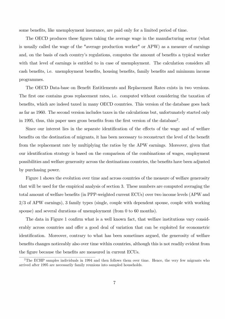
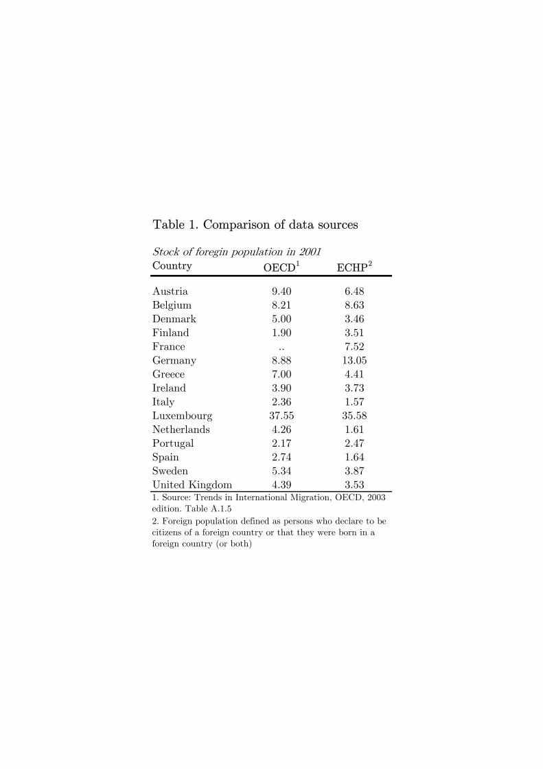
We adopt this dual definition because it allows to cover the largest set of countries (e.g. there
is no information on citizenship for Germany but migration trajectories are reported) and also
because it is the one that performs better in comparison with official migration data from the
OECD, as shown in Table 11. There still exist discrepancies, which are sometimes large, between
our estimates of the stock of foreign population and the official data but, considering that the
ECHP is not explicitly designed for the study of migration and that the sample of migrants in some
countries is relatively small, the overall performance of the ECHP on this issue can be considered
satisfactory.
Another important piece of information available from the ECHP is the year of arrival in the
current country of residence, which allows to match to each individual the economic conditions of
all possible destination countries at the time the decision to migrate was taken. However, since data
on welfare generosity and macroeconomic conditions are not easily available for the very past years,
only migrants who arrived in the country of present residence in or after 1970 have been considered.
The sample has also been restricted to individuals who were aged between 15 and 55 at the time
of arrival. Unfortunately, the data on welfare generosity are not available for Luxembourg and this
country has been dropped from the sample used in section 3 (some figures for this country will still
be produced in section 4).
1In an earlier version, we defined migrants simply as those who were born abroad and had lived abroad beforecoming to the country of current residence. The empirical estimates produced using this alternative definition werequalitatively similar to the ones presented here. However, the dual definition used in the current version of this paperallows to identify a larger group of migrants and thus to produce more precise estimates. Moreover, it also replicatesthe official statistics more closely (see Table 1).
5
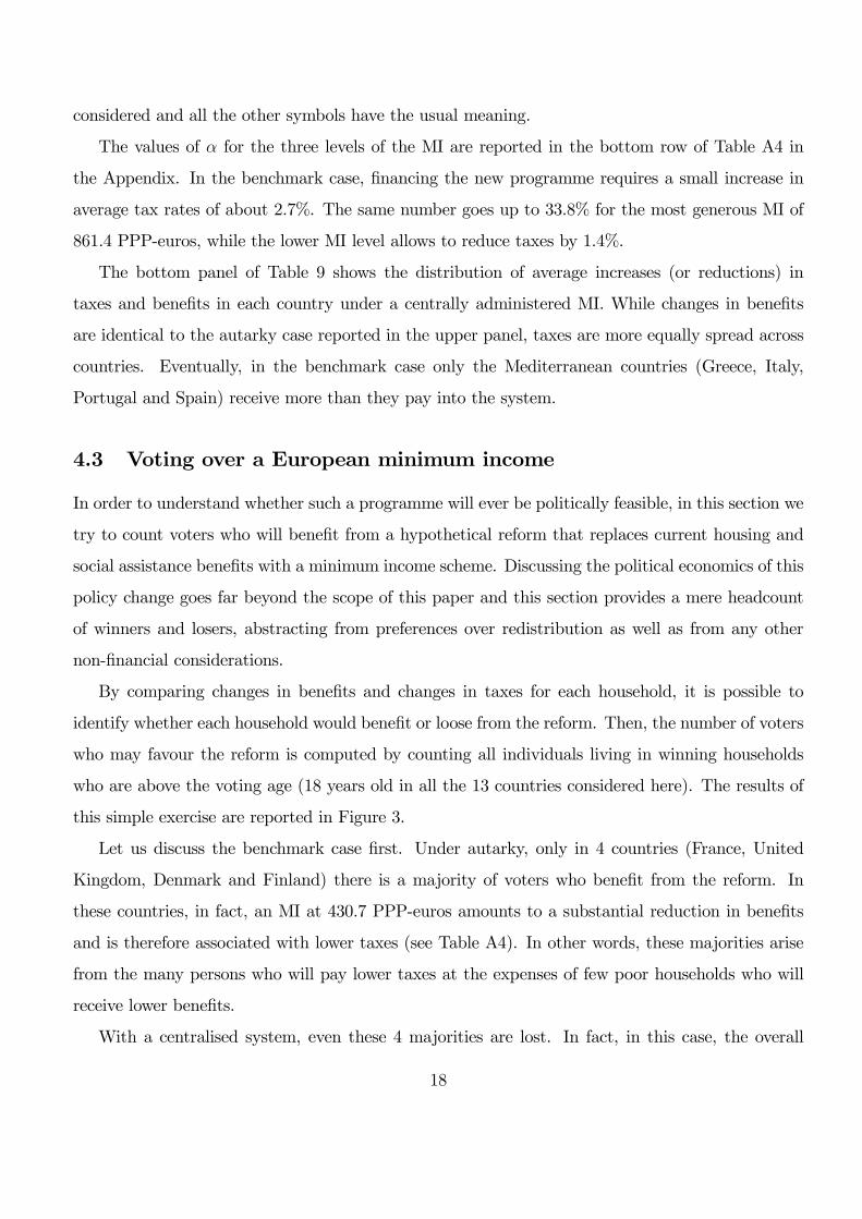
Eventually, the empirical exercise of section 3 uses a sample of 3038 migrants from outside the
pre-enlargement EU-15, distributed in 14 countries of the European Union according to Table 2.
Summary statistics are also shown in Table 2, together with the distribution of the years of arrival
for each destination country.
The data show that migrants usually move in their late twenties and that they are rather evenly
distributed by gender with some countries, like Italy, where the presence of women is particularly
high (probably because they cluster into female-dominated occupations, like housekeeping and nurs-
ing). The distribution of education is more varied with the Nordic and the Anglo-Saxon countries
attracting the most educated migrants (with some exceptions like Greece and Spain).
For many countries the first nineties have been the years of most intense immigration but the
data indicate a large variation in the sequence of migration waves across countries, resulting in a
rather even distribution of arrivals for the entire Union.
It is worth mentioning here a couple of caveats of this sample. It is a known fact that some
countries are often used as a port of entry (e.g. Italy, Spain, Greece, etc.) and the final destination
of migration might not be the one observed in the data. The ECHP does not contain questions
about the intention to leave the country in the future. We can only argue that most immigrants,
who only transit in one country with the intention to move to another one, typically do that illegally
and, even if they register, they remain in the port-of-entry country only for a very short period.
Thus, they are very unlikely to be sampled in the ECHP. This also implies, however, that most
illegal migrants will not be covered by our analysis.
2.2 OECD Data-base on Benefit Entitlements and Replacement Rates
Data on welfare generosity come from the OECD Data-base on Benefit Entitlements and Replace-
ment Rates, which has been often used in the literature to describe the generosity as well as other
characteristics of the welfare systems in the countries of the OECD.
In particular, this database measures the generosity of welfare by computing the ratio between
income out of work - i.e. from welfare benefits - and income in work - i.e. some measure of
the average wage. These figures, called replacement rates, are computed for several family types
(single, couple with and without dependants), income levels (average earnings or 2/3 of the average
earnings) and various durations of unemployment (from the first month up to the 60th month), as
6
some benefits, like unemployment insurance, are paid only for a limited period of time.
The OECD produces these figures taking the average wage in the manufacturing sector (what
is usually called the wage of the "average production worker" or APW) as a measure of earnings
and, on the basis of each country’s regulations, computes the amount of benefits a typical worker
with that level of earnings is entitled to in case of unemployment. The calculation considers all
cash benefits, i.e. unemployment benefits, housing benefits, family benefits and minimum income
programmes.
The OECD Data-base on Benefit Entitlements and Replacement Rates exists in two versions.
The first one contains gross replacement rates, i.e. computed without considering the taxation of
benefits, which are indeed taxed in many OECD countries. This version of the database goes back
as far as 1960. The second version includes taxes in the calculations but, unfortunately started only
in 1995, thus, this paper uses gross benefits from the first version of the database2.
Since our interest lies in the separate identification of the effects of the wage and of welfare
benefits on the destination of migrants, it has been necessary to reconstruct the level of the benefit
from the replacement rate by multiplying the ratios by the APW earnings. Moreover, given that
our identification strategy is based on the comparison of the combinations of wages, employment
possibilities and welfare generosity across the destinations countries, the benefits have been adjusted
by purchasing power.
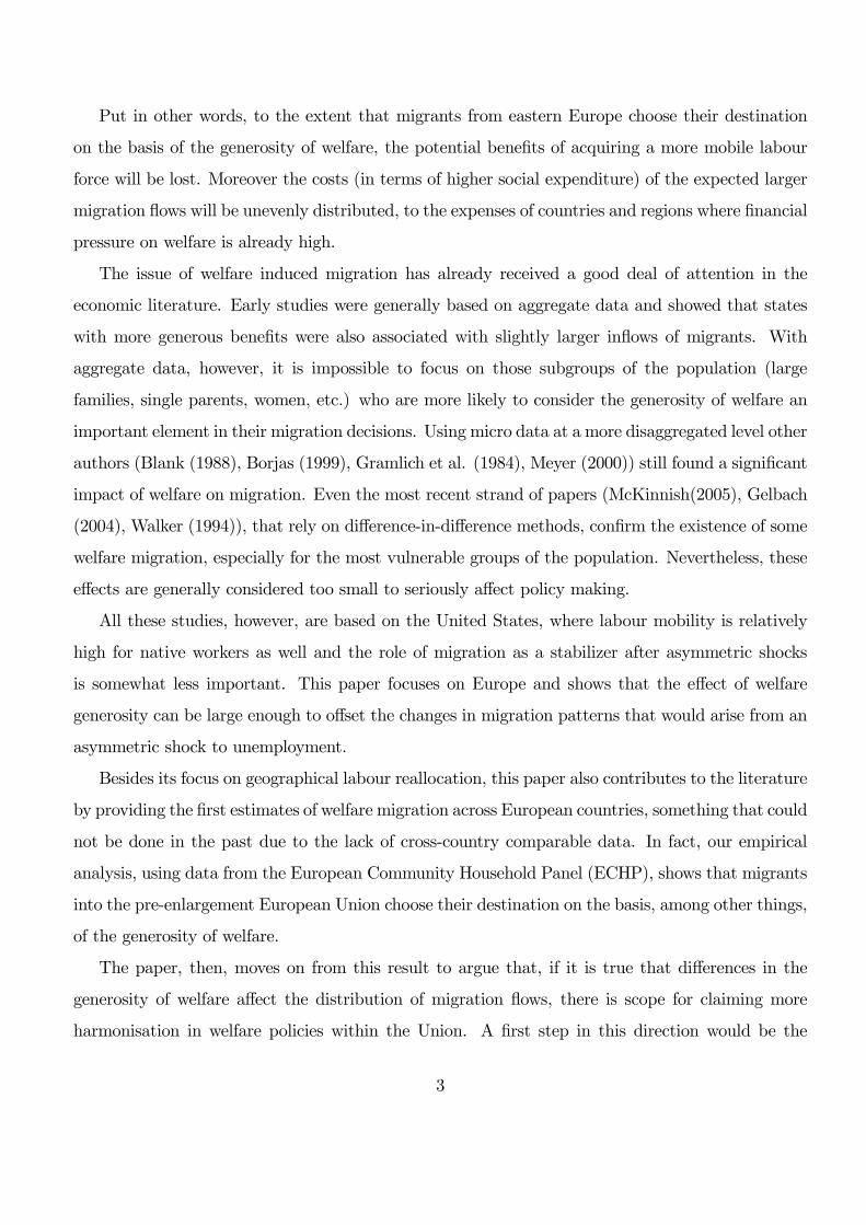
Figure 1 shows the evolution over time and across countries of the measure of welfare generosity
that will be used for the empirical analysis of section 3. These numbers are computed averaging the
total amount of welfare benefits (in PPP-weighted current ECUs) over two income levels (APW and
2/3 of APW earnings), 3 family types (single, couple with dependent spouse, couple with working
spouse) and several durations of unemployment (from 0 to 60 months).
The data in Figure 1 confirm what is a well known fact, that welfare institutions vary consid-
erably across countries and offer a good deal of variation that can be exploited for econometric
identification. Moreover, contrary to what has been sometimes argued, the generosity of welfare
benefits changes noticeably also over time within countries, although this is not readily evident from
the figure because the benefits are measured in current ECUs.
2The ECHP samples individuals in 1994 and then follows them over time. Hence, the very few migrants whoarrived after 1995 are necessarily family reunions into sampled households.
7
3 Welfare generosity and the choice of migration: an em-
pirical model
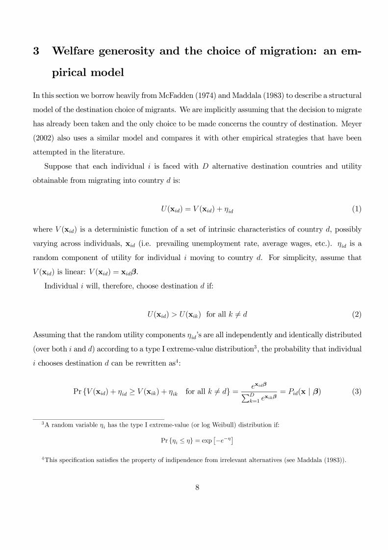
In this section we borrow heavily fromMcFadden (1974) andMaddala (1983) to describe a structural
model of the destination choice of migrants. We are implicitly assuming that the decision to migrate
has already been taken and the only choice to be made concerns the country of destination. Meyer
(2002) also uses a similar model and compares it with other empirical strategies that have been
attempted in the literature.
Suppose that each individual i is faced with D alternative destination countries and utility
obtainable from migrating into country d is:
U(xid) = V (xid) + ηid (1)
where V (xid) is a deterministic function of a set of intrinsic characteristics of country d, possibly
varying across individuals, xid (i.e. prevailing unemployment rate, average wages, etc.). ηid is a
random component of utility for individual i moving to country d. For simplicity, assume that
V (xid) is linear: V (xid) = xidβ.
Individual i will, therefore, choose destination d if:
U(xid) > U(xik) for all k 6= d (2)
Assuming that the random utility components ηid’s are all independently and identically distributed
(over both i and d) according to a type I extreme-value distribution3, the probability that individual
i chooses destination d can be rewritten as4:
Pr {V (xid) + ηid ≥ V (xik) + ηik for all k 6= d} = exidβPDk=1 e
xikβ= Pid(x | β) (3)
3A random variable ηi has the type I extreme-value (or log Weibull) distribution if:
Pr {ηi ≤ η} = exp£−e−η
¤4This specification satisfies the property of indipendence from irrelevant alternatives (see Maddala (1983)).
8

Equation (3) clearly indicates that the identification in this model comes from comparing the
same individual faced with different alternative destinations. In fact, since each individual i is only
observed taking one destination d, all individual characteristics that do not vary across countries
(age, education, etc.) are collinear and cancel out in the specification of Pid.
The log-likelihood function for a sample of N migrants facing D destinations can, then, be
written as:
L(β) =NXi=1
DXd=1
fid logPid(x | β) (4)
where fid = 1 if individual i chooses destination d and zero otherwise.
The model described in equation (4) is estimated under various specifications of the utility
function U(xid). Initially, we simply want to replicate the known result that employment possibilities
and wages are the main determinants of the destination of migration. In order to test this hypothesis,
the set of destination attributes, xid, includes the unemployment rate and the average real wage
in each destination country d corresponding to the year in which individual i settled into his/her
country of current residence.
As additional controls, we always include a set of destination country dummies and 4 time
period dummies for arrivals before 1980, between 1980 and 1985, between 1985 and 1990 and after
1990. These two sets of dummies are also interacted, thus allowing destination-specific effects (the
strictness of migration laws, networks of migrants already present in the country, etc.) to change
at discrete time intervals5.
Results are shown in the first column of Table 3 and indeed confirm that migrants tend to go
into countries with lower unemployment rates and higher real wages. The second column of Table
3 repeats the same estimation adding to the set of explanatory variables the interactions between
the log of the unemployment rate and of the wage with some individual characteristics, to check
whether some groups are particularly sensitive to the conditions of the labour market.
The results indicate that the migration decisions of the more educated are less affected by
unemployment and wages, perhaps because they generally have good changes of finding a job
and their actual earnings are less correlated with the average. Those who migrate early in their
5Our results are robust to alternative specifications of the time effects and their interactions with the destinationcountries fixed-effects.
9
lives (before 25 years old) also appear to attach less importance to the wage, probably because
they see their experience in a different country also as an investment in human capital and are,
therefore, willing to accept lower wages (compared to what they could earn in other destinations).
Interestingly, there seems to be no detectable differences between men and women.
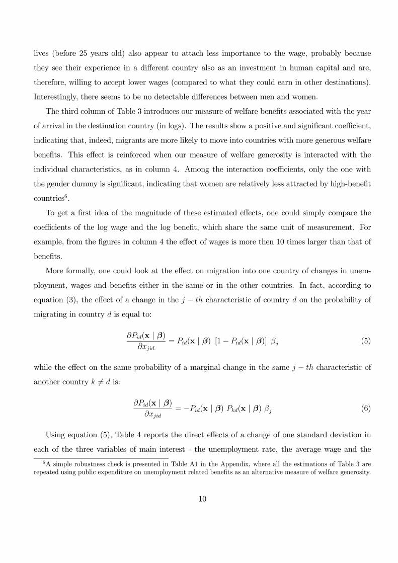
The third column of Table 3 introduces our measure of welfare benefits associated with the year
of arrival in the destination country (in logs). The results show a positive and significant coefficient,
indicating that, indeed, migrants are more likely to move into countries with more generous welfare
benefits. This effect is reinforced when our measure of welfare generosity is interacted with the
individual characteristics, as in column 4. Among the interaction coefficients, only the one with
the gender dummy is significant, indicating that women are relatively less attracted by high-benefit
countries6.
To get a first idea of the magnitude of these estimated effects, one could simply compare the
coefficients of the log wage and the log benefit, which share the same unit of measurement. For
example, from the figures in column 4 the effect of wages is more then 10 times larger than that of
benefits.
More formally, one could look at the effect on migration into one country of changes in unem-
ployment, wages and benefits either in the same or in the other countries. In fact, according to
equation (3), the effect of a change in the j − th characteristic of country d on the probability of
migrating in country d is equal to:
∂Pid(x | β)∂xjid
= Pid(x | β) [1− Pid(x | β)] βj (5)
while the effect on the same probability of a marginal change in the same j − th characteristic of
another country k 6= d is:
∂Pid(x | β)∂xjid
= −Pid(x | β) Pkd(x | β) βj (6)
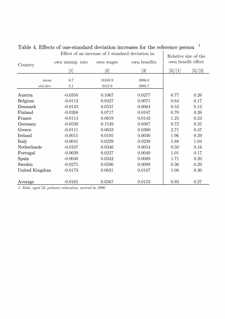
Using equation (5), Table 4 reports the direct effects of a change of one standard deviation in
each of the three variables of main interest - the unemployment rate, the average wage and the
6A simple robustness check is presented in Table A1 in the Appendix, where all the estimations of Table 3 arerepeated using public expenditure on unemployment related benefits as an alternative measure of welfare generosity.
10

generosity of welfare - as implied by the estimates in column 4 of Table 3 and computed for a
representative person (male, aged 25, with primary education and arrived in 1990). As indicated
by the last two columns, the effect of a one-standard deviation change in the unemployment rate
(which is a huge change of more than 3 percentage points) is only in a few countries comparable to
a similar change in welfare benefits.
Perhaps, it is easier to interpret the ratio between the change in wages and benefits, since they
share the same unit of measurement. The ratios in the last column of Table 4 show that increasing
welfare benefits by one-standard deviation induces an increase in migration flows that is on average
only 27% of what a similar change in wages would have generated. Only in Italy the size of the
two effects is comparable but in this country benefits are extremely low and the simulated change
of one-standard deviation leads to benefits more than 7 times higher.
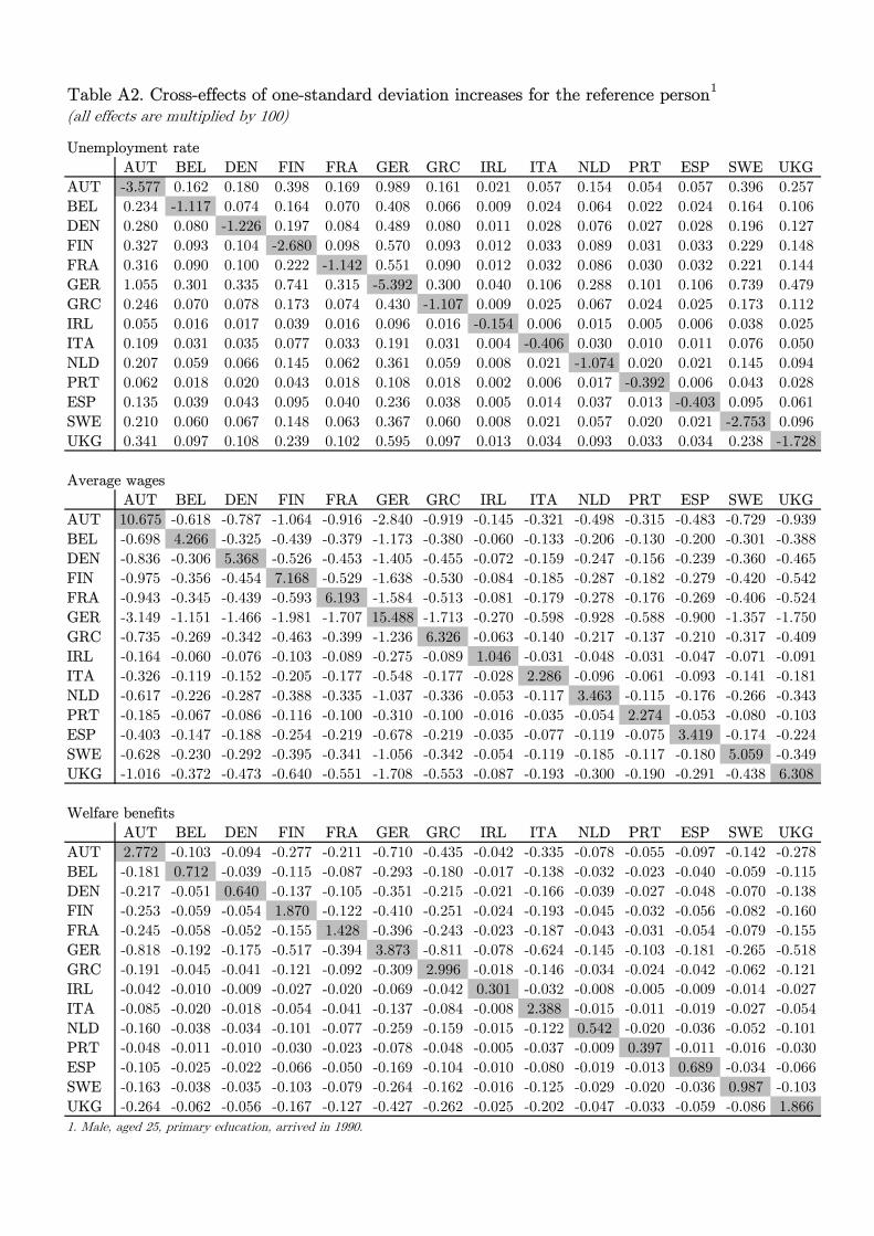
The full matrix of both direct and cross- marginal effects computed for the reference person
according to equations (5) and (6) is reported in Table A2 in the appendix. These numbers are
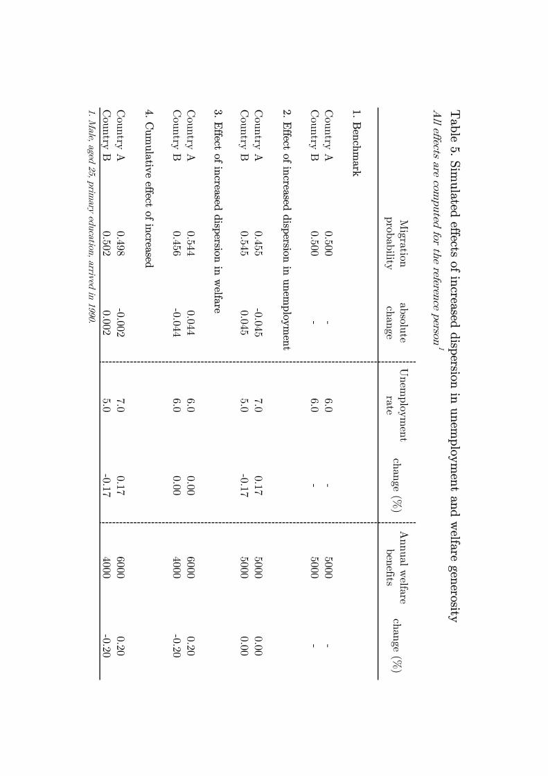
useful to conduct the thought experiment reported in Table 5, which tries to relate these estimates
to the initial issue of labour reallocation.
Suppose that there are only two possible destination countries, A and B, and that they are
initially identical, with unemployment equal to 6% and welfare benefits of 5,000 euros per year
(approximately the averages across the 14 countries used for the estimation). Migration flows will,
then, be evenly distributed across the two countries, with the reference person migrating to any
of them with a probability of 50%. This is the benchmark situation described in the first panel of
Table 5.
Suppose now - panel 2 in Table 5 - that the two countries are hit by an asymmetric shock to
unemployment (assume, for simplicity, that wages are rigid) which goes up to 7% in country A and
down to 5% in country B. The estimates of Table 3 predicts that this will generate a reduction
of about 0.045 in the flow of migrants to country A and a symmetric increase for country B. This
change in migration flows would, then, help to absorb the shock even if no native worker would
move from A to B.
What would happen if benefits were changed too? Panel 3 computes the effect on the migration
probabilities of a 20% increase in country A’s benefits associated with an identical and simultaneous
reduction in country B. The results indicate that the effect would be very similar that of the change
11
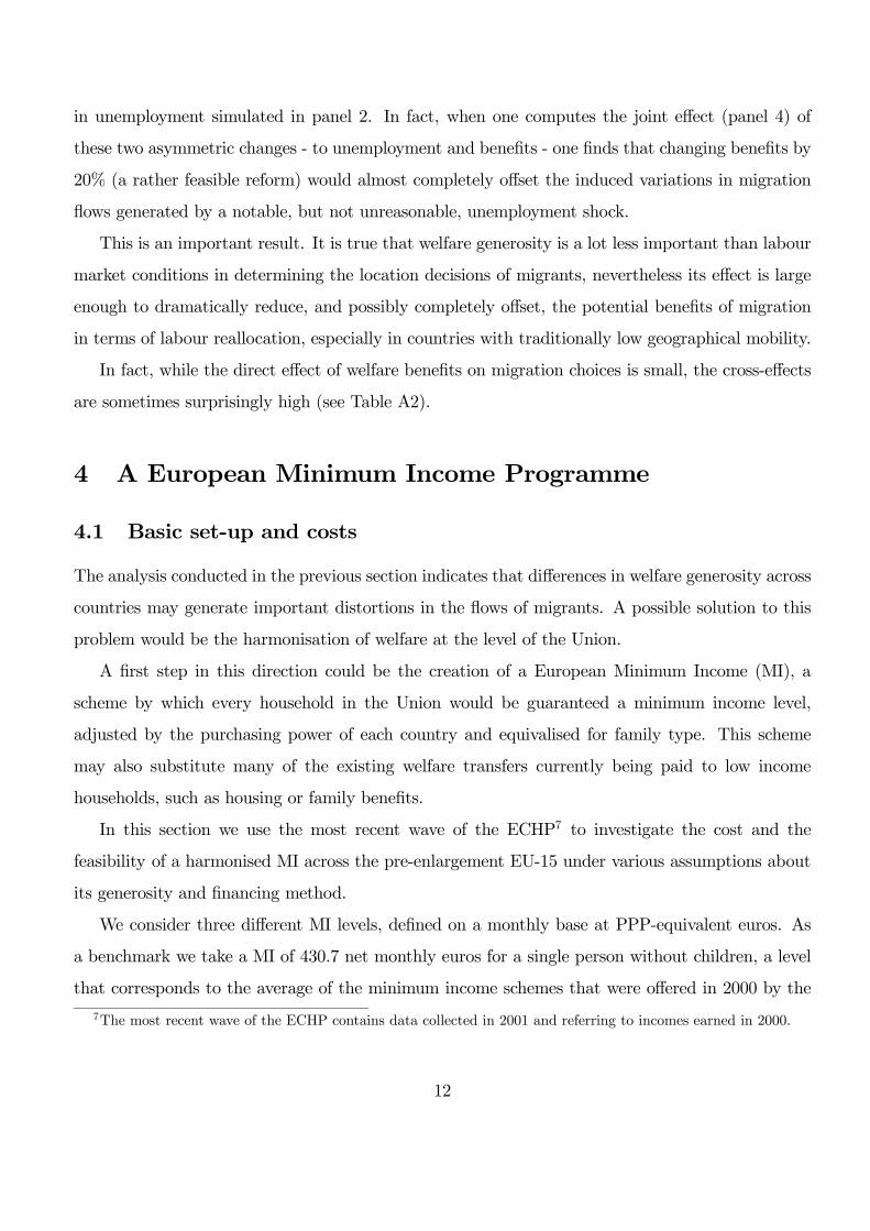
in unemployment simulated in panel 2. In fact, when one computes the joint effect (panel 4) of
these two asymmetric changes - to unemployment and benefits - one finds that changing benefits by
20% (a rather feasible reform) would almost completely offset the induced variations in migration
flows generated by a notable, but not unreasonable, unemployment shock.
This is an important result. It is true that welfare generosity is a lot less important than labour
market conditions in determining the location decisions of migrants, nevertheless its effect is large
enough to dramatically reduce, and possibly completely offset, the potential benefits of migration
in terms of labour reallocation, especially in countries with traditionally low geographical mobility.
In fact, while the direct effect of welfare benefits on migration choices is small, the cross-effects
are sometimes surprisingly high (see Table A2).
4 A European Minimum Income Programme
4.1 Basic set-up and costs
The analysis conducted in the previous section indicates that differences in welfare generosity across
countries may generate important distortions in the flows of migrants. A possible solution to this
problem would be the harmonisation of welfare at the level of the Union.
A first step in this direction could be the creation of a European Minimum Income (MI), a
scheme by which every household in the Union would be guaranteed a minimum income level,
adjusted by the purchasing power of each country and equivalised for family type. This scheme
may also substitute many of the existing welfare transfers currently being paid to low income
households, such as housing or family benefits.
In this section we use the most recent wave of the ECHP7 to investigate the cost and the
feasibility of a harmonised MI across the pre-enlargement EU-15 under various assumptions about
its generosity and financing method.
We consider three different MI levels, defined on a monthly base at PPP-equivalent euros. As
a benchmark we take a MI of 430.7 net monthly euros for a single person without children, a level
that corresponds to the average of the minimum income schemes that were offered in 2000 by the
7The most recent wave of the ECHP contains data collected in 2001 and referring to incomes earned in 2000.
12
countries of the Union8. Details on how this average has been calculated are provided in Table A3
in the Appendix. A lower - 215.35 monthly PPP euros, equal to 1/2 of the average - and a higher -
861.4 monthly PPP euros, equal to twice the average - MI levels are also considered for comparison
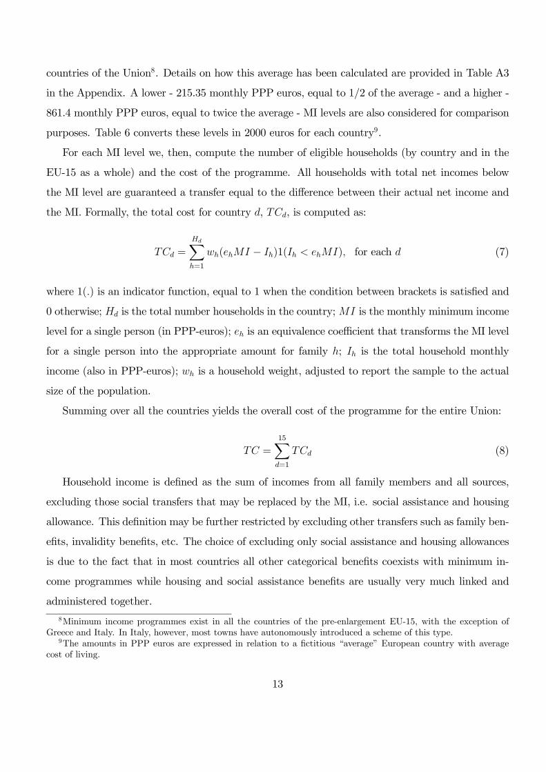
purposes. Table 6 converts these levels in 2000 euros for each country9.
For each MI level we, then, compute the number of eligible households (by country and in the
EU-15 as a whole) and the cost of the programme. All households with total net incomes below
the MI level are guaranteed a transfer equal to the difference between their actual net income and
the MI. Formally, the total cost for country d, TCd, is computed as:
TCd =
HdXh=1
wh(ehMI − Ih)1(Ih < ehMI), for each d (7)
where 1(.) is an indicator function, equal to 1 when the condition between brackets is satisfied and
0 otherwise; Hd is the total number households in the country;MI is the monthly minimum income
level for a single person (in PPP-euros); eh is an equivalence coefficient that transforms the MI level
for a single person into the appropriate amount for family h; Ih is the total household monthly
income (also in PPP-euros); wh is a household weight, adjusted to report the sample to the actual
size of the population.
Summing over all the countries yields the overall cost of the programme for the entire Union:
TC =15Xd=1
TCd (8)
Household income is defined as the sum of incomes from all family members and all sources,
excluding those social transfers that may be replaced by the MI, i.e. social assistance and housing
allowance. This definition may be further restricted by excluding other transfers such as family ben-
efits, invalidity benefits, etc. The choice of excluding only social assistance and housing allowances
is due to the fact that in most countries all other categorical benefits coexists with minimum in-
come programmes while housing and social assistance benefits are usually very much linked and
administered together.
8Minimum income programmes exist in all the countries of the pre-enlargement EU-15, with the exception ofGreece and Italy. In Italy, however, most towns have autonomously introduced a scheme of this type.
9The amounts in PPP euros are expressed in relation to a fictitious “average” European country with averagecost of living.
13

The equivalence scale we adopt is the one officially used by the OECD, which equals one for single
adults and adds 0.7 for any additional adult and 0.5 for any additional child below 14 years-old.
Notice that we are neglecting any labour supply response. In principle, in fact, some households
may react to the introduction of the new scheme by reducing their labour supply in order to become
eligible for the programme. Taking this effect into consideration would require several additional
pieces of information which are not readily available from the ECHP, the most important being gross
incomes and labour supply elasticities. While gross incomes can be reasonably calculated using a
net/gross factor at the household level (provided in the ECHP and which is used in the following
subsection), the estimation of labour supply at the household level would be very problematic and
goes beyond the scope of this paper.
Moreover, we believe that allowing for labour supply response would not change our results
significantly for two reasons. First, the size of the response depends on the wage elasticity of labour
supply, which we know from many empirical studies to be very low, especially in Europe (Blundell
et al. (2000)). Second, most of the effect is likely to arise from changes in participation decisions
rather than changes in the supply of hours of already employed workers. And, in our scheme,
changes in the tax-benefit position of households around the participation margin are very limited
because only households with net disposable incomes exceeding the MI threshold by at least 20%
are subject to higher (or lower) taxation (see the following subsection).
Overall, the inclusion of labour supply responses in this analysis would require a number of ad
hoc assumptions that will make the results questionable. For these reasons we prefer to keep things
simple and present results from a static analysis.
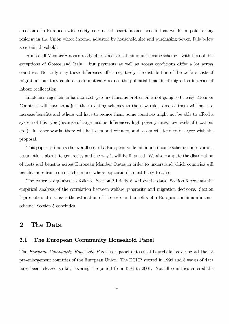
Figure 2 shows the number of eligible households and the related annual costs for the three MI
levels that we consider for the entire EU-15. These figures are plotted in percentage terms relative
to the total number of households in the EU-15 and to the 2000 expenditure for housing and social
assistance benefits, respectively. The data labels in the figure, instead, refer to the absolute numbers
of recipient households and the absolute cost of the scheme.
At the lowest MI level, about 2.8 millions households (corresponding to about 1.8% of all EU-15
households) receive a transfer from the system with an aggregate cost of approximately 5.4 billions
of euros (corresponding to 14% of current expenditure). These numbers increase rapidly as the
MI level approaches the mean of the income distribution. With a minimum income equal to the
14
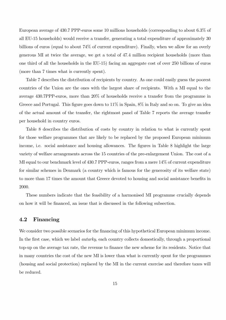
European average of 430.7 PPP-euros some 10 millions households (corresponding to about 6.3% of
all EU-15 households) would receive a transfer, generating a total expenditure of approximately 30
billions of euros (equal to about 74% of current expenditure). Finally, when we allow for an overly
generous MI at twice the average, we get a total of 47.4 million recipient households (more than
one third of all the households in the EU-15) facing an aggregate cost of over 250 billions of euros
(more than 7 times what is currently spent).
Table 7 describes the distribution of recipients by country. As one could easily guess the poorest
countries of the Union are the ones with the largest share of recipients. With a MI equal to the
average 430.7PPP-euros, more than 20% of households receive a transfer from the programme in
Greece and Portugal. This figure goes down to 11% in Spain, 8% in Italy and so on. To give an idea
of the actual amount of the transfer, the rightmost panel of Table 7 reports the average transfer
per household in country euros.
Table 8 describes the distribution of costs by country in relation to what is currently spent
for those welfare programmes that are likely to be replaced by the proposed European minimum
income, i.e. social assistance and housing allowances. The figures in Table 8 highlight the large
variety of welfare arrangements across the 15 countries of the pre-enlargement Union. The cost of a
MI equal to our benchmark level of 430.7 PPP-euros, ranges from a mere 14% of current expenditure
for similar schemes in Denmark (a country which is famous for the generosity of its welfare state)
to more than 17 times the amount that Greece devoted to housing and social assistance benefits in
2000.
These numbers indicate that the feasibility of a harmonised MI programme crucially depends
on how it will be financed, an issue that is discussed in the following subsection.
4.2 Financing
We consider two possible scenarios for the financing of this hypothetical European minimum income.
In the first case, which we label autarky, each country collects domestically, through a proportional
top-up on the average tax rate, the revenue to finance the new scheme for its residents. Notice that
in many countries the cost of the new MI is lower than what is currently spent for the programmes
(housing and social protection) replaced by the MI in the current exercise and therefore taxes will
be reduced.
15
The alternative method, labelled centralised, is one in which the programme is financed through
a proportional top-up tax identical for all households regardless of their country of residence. The
structure of the top-up tax maintains the degree of progressivity of the tax system at the European
level (or within countries in the autarky case).
While autarky generates redistribution of resources only within countries, in the centralised
system rich countries pay more into the new scheme than they receive, generating a considerable
redistribution of resources also across countries.
These two methods share the common feature that additional taxes will be levied only on those
households whose income exceeds the MI threshold by at least 20%. This ensures that the marginal
tax rates around the MI threshold are not excessively high and discourage employment. More
complicated mechanisms could be envisaged for this particular purpose, for example a gradual
withdrawal of the benefit as household income increases10.
In autarky, then, taxes will be increased (or decreases) by the same factor αd for all households
in country d in such a way to cover the additional (or lower) tax revenue necessary to finance the
new programme for the residents in country d. αd is computed in order to guarantee that the
increase in taxes covers the additional revenue required to finance the MI, as stated in the following
equation:
"(1 + αd)
HdXh=1
whthY1h 1(Ih > 1.2 · eh ·MI)
#| {z }
total revenue after-reform
−"
HdXh=1
whthY0h
#| {z }
total revenue pre reform
= TCd − SAd| {z }additional revenue required
(9)
where th is the average tax rate for family h, Yh is gross total income for household h and SAd
is current (2000) expenditure for social assistance and housing benefits. All other symbols have
been described above. The superscripts 0 and 1 on Yh indicate that after the reform some sources
of income have been eliminated. In fact, the pre-reform gross income, Y 0h , includes also social
assistance and housing benefits, while these are excluded from Y 1h , the post-reform gross income.
We compute gross incomes and the average tax rates using the net-to-gross factor provided in the
ECHP. This variable is only available at the level of the household and allows to reconstruct, with
some approximation, total household income from total net income and, consequently, to recover
10The distribution of winners and losers is, however, remarkably stable to changes in this exemption mechanism.
16
the average tax rate. Unfortunately, this information is not available for Luxembourg and Sweden
which have been excluded from these calculations.
From equation (9) it is immediate to derive an expression for αd:
αd =(TCd − SAd) +
PHd
h=1whthY0hPHd
h=1whthY 1h 1(Ihd > 1.2 · ehd ·MI)
− 1 (10)
The values of αd for each country are reported in Table A4 in the Appendix, while the upper panel
of Table 9 describes the average increase (or reduction) in taxes and benefits in each country under
autarky.
In the benchmark case of an MI equal to 430.7 PPP-euros, the Mediterranean countries (Greece,
Italy, Portugal and Spain) and Ireland experience an increase in average benefits while in all the
other countries benefits are reduced.
Normally, increases in average benefits are associated with higher taxes and vice versa. However,
in some countries (Austria, Belgium, Germany and the Netherlands) the introduction of the MI
leads to lower average benefits and higher taxes. In fact, spreading the cost of the new programme
only on households with incomes exceeding the threshold by at least 20% reduces the tax base and
requires higher average rates even when benefits are lowered.
The alternative scenario, i.e. the centralised system, is based on the same principle but operates
at the level of the entire European Union (which, with the exclusion of Luxembourg and Sweden,
is now a EU-13). In practice, in this scenario all member states would transfer to a central body
what they are currently spending for housing and social assistance benefits. This fictitious central
administration would, then, use these resources to pay MI transfers to all households who meet
the eligibility criteria and charge additional taxes, through a common proportional increase in the
average tax rate, should additional resources be needed. If total current expenditure is, instead, in
excess of the cost of the MI, taxes would be reduced via the same system.
Hence, there is now a unique α applied to all households in the EU-13, regardless of their country
of residence:
α =(TC − SA) +
PHh=1whthY
0hPH
h=1whthY 1h 1(Ih > 1.2 · eh ·MI)
− 1 (11)
where H is the total number of households in the entire Union (i.e. H =P
dHd), SA =P
d SAd
is the sum of current expenditure for housing and social assistance benefits in all the 13 countries
17
considered and all the other symbols have the usual meaning.
The values of α for the three levels of the MI are reported in the bottom row of Table A4 in
the Appendix. In the benchmark case, financing the new programme requires a small increase in
average tax rates of about 2.7%. The same number goes up to 33.8% for the most generous MI of
861.4 PPP-euros, while the lower MI level allows to reduce taxes by 1.4%.
The bottom panel of Table 9 shows the distribution of average increases (or reductions) in
taxes and benefits in each country under a centrally administered MI. While changes in benefits
are identical to the autarky case reported in the upper panel, taxes are more equally spread across
countries. Eventually, in the benchmark case only the Mediterranean countries (Greece, Italy,
Portugal and Spain) receive more than they pay into the system.
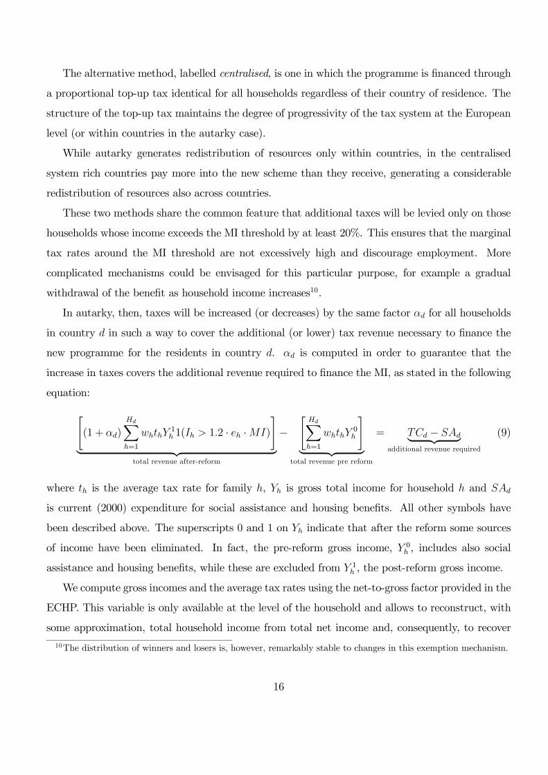
4.3 Voting over a European minimum income
In order to understand whether such a programme will ever be politically feasible, in this section we
try to count voters who will benefit from a hypothetical reform that replaces current housing and
social assistance benefits with a minimum income scheme. Discussing the political economics of this
policy change goes far beyond the scope of this paper and this section provides a mere headcount
of winners and losers, abstracting from preferences over redistribution as well as from any other
non-financial considerations.
By comparing changes in benefits and changes in taxes for each household, it is possible to
identify whether each household would benefit or loose from the reform. Then, the number of voters
who may favour the reform is computed by counting all individuals living in winning households
who are above the voting age (18 years old in all the 13 countries considered here). The results of
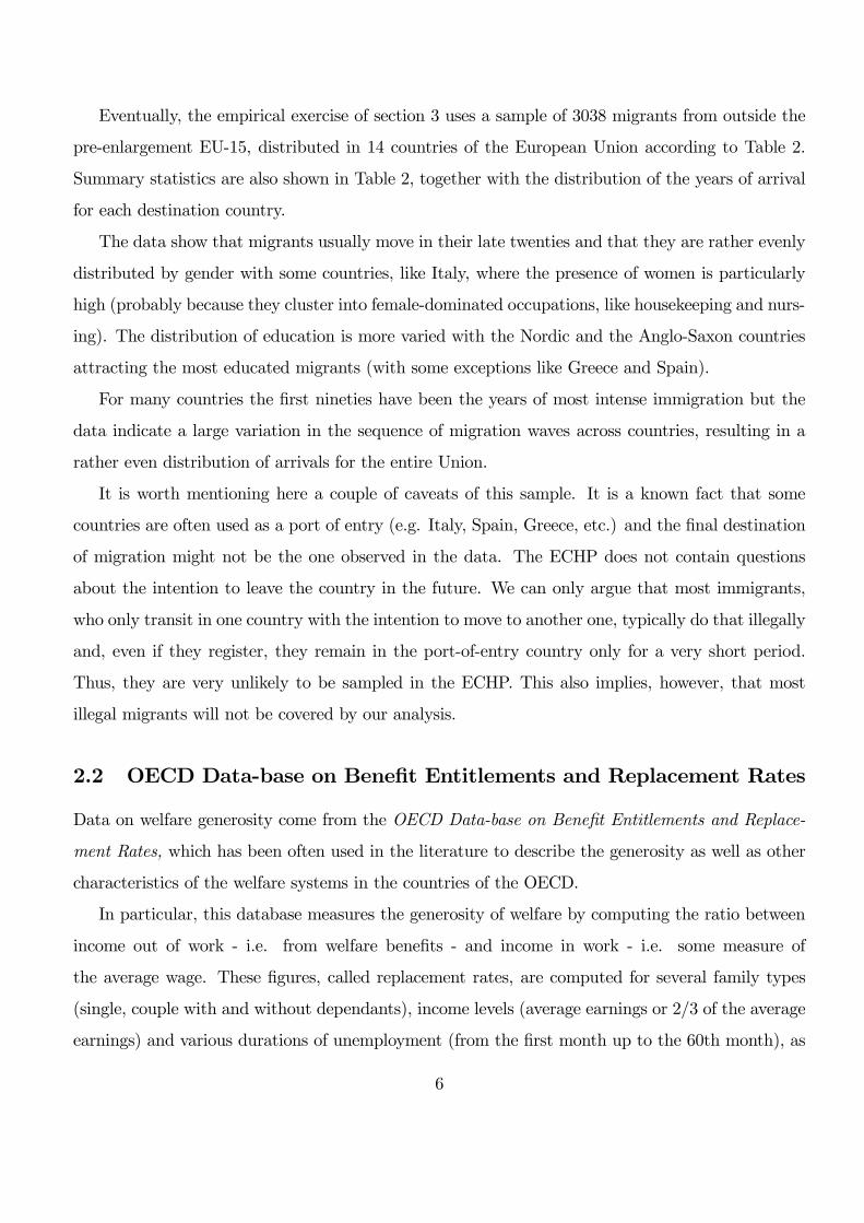
this simple exercise are reported in Figure 3.
Let us discuss the benchmark case first. Under autarky, only in 4 countries (France, United
Kingdom, Denmark and Finland) there is a majority of voters who benefit from the reform. In
these countries, in fact, an MI at 430.7 PPP-euros amounts to a substantial reduction in benefits
and is therefore associated with lower taxes (see Table A4). In other words, these majorities arise
from the many persons who will pay lower taxes at the expenses of few poor households who will
receive lower benefits.
With a centralised system, even these 4 majorities are lost. In fact, in this case, the overall
18

cost of the programme is spread equally across all member countries, thus also rich households in
France, United Kingdom, Denmark and Finland will end up paying higher taxes.
The highest MI level, on the contrary, will have a potential majority of supporters only in the
poorest countries of the Union, i.e. Greece and Portugal. In this case, in fact, the benefit is so high
compared to the distribution of incomes that very many households will receive it at the expenses
of a few very rich individuals who will pay very high taxes to finance it.
Notice that in this case the distribution of winners is unchanged, regardless of whether the
scheme is financed locally or centrally. With benefits this high, in fact, taxes have to be increased
in all countries. All tax-payers are losers and all benefit recipients are winners. In a centralised
system, losers in rich countries will simply loose more.
Finally, the solution that seems to attract most potential support is the lowest MI. In this case,
in fact, the reform generates reductions in social transfers in almost all countries (apart from the
Mediterranean ones) and is thus associated with substantial and widespread tax rebates (see Table
A4). Only in Greece, Italy, Portugal and Spain, even an MI at 215.35 PPP-euros is more generous
than current housing and social assistance transfers and, thus, requires higher taxes in autarky.
Notice, in fact, that, when the lower MI is financed centrally, a majority in favour of the reform can
be reached also in the Mediterranean countries.
5 Conclusions
The results of this paper suggest that the generosity of the welfare state may act as a migration
magnet across the countries of the European Union. This finding supports the concerns expressed
by many observers of a potential threat to the welfare state posed by the enlargement of the Union.
On the other hand, however, the same estimates indicate that the size of these welfare magnets is
relatively low, compared to the role of labour market conditions, such as the unemployment rate
and the level of wages.
The issue, then, is not whether migrants will flood into countries with generous welfare benefits,
but to what extent the variation in the welfare institutions across the countries of the Union will
generate distortions in the flows of migration. The empirical analysis conducted in the first part
of this paper shows that these distortions can be large enough to reduce, and possibly completely
19
offset, the potential benefits of acquiring a more mobile labour force. This is, in fact, one of
the most important advantages that increased migration can offer to the countries of the pre-
enlargement Union, an area where native workers traditionally move a lot less than, for example,
North-Americans.
The second part of the paper explores the feasibility of one possible solution to this problem:
the creation of a more harmonised welfare system across the Union through the introduction of a
uniform minimum income programme. Under various assumptions about the generosity and the
method of financing, we compute the costs and the benefits of such a scheme for each country of
the pre-enlargement Union.
The results indicate that, for a minimum income set at the average of similar programmes
adopted in the EU, the new system would cost about three quarters of what is currently spent on
housing and social assistance benefits and, considering that a programme of this type could easily
replace these benefits, its cost does not seem unbearable.
The distribution, rather than the level, of the costs is more likely to create obstacles to its actual
implementation. Imposing a uniform minimum income to all countries and requiring each of them
to autonomously finance its own payments does not seem to obtain a majority that would support
such a reform (if voters care only about their incomes). To make the new system politically feasible
a certain degree of redistribution might be required, with some countries receiving more than they
pay. A minimum income at a lower-than-average level financed via a centralised system is likely
to obtain support from a majority in each country as well as in the entire Union. Our estimates
indicate that the most generous MI level than is politically feasible is in the order of approximately
320 PPP-euros for a single individual.
References
[1] Alvarez-Plata, Patricia, Herbert Brücker and Boriss Siliverstovs. 2003. Potential Migration from
Central and Eastern Europe into the EU-15 — An Update. Report for European Commission,
DG Employment and Social Affairs, Brussels.
[2] Bartel, Ann P. 1989. ”Where Do the New U.S. Immigrants Live?” Journal of Labour Economics
7(4): 371-391.
20
[3] Blank, Rebecca M. 1988. "The Effect of Welfare and Wage Levels on the Location Decisions
of Female-Headed Households." Journal of Urban Economics 24(2): 186-211.
[4] Blundell, Richard, and MaCurdy, Thomas E. 2000. “Labor Supply: A Review of Alternative
Approaches.” In Handbook of Labor Economics, vol. 3a, edited by Orley Ashenfelter and David
Card, pp. 1560—1695. Amsterdam: North-Holland.
[5] Boeri, Tito, Gordon H. Hanson and Barry McCormick. 2002. Immigration Policy and the
Welfare System. Oxford University Press.
[6] Boeri, Tito and Herbert Brücker. 2001.The Impact of Eastern Enlargement on Employment and
Labour Markets in the EU Member States. Report for European Commission, DG Employment
and Social Affairs, Brussels.
[7] Borjas, George. 1999. ”Immigration andWelfare Magnets.” Journal of Labour Economics 17(4):
607-637.
[8] Gelbach, Jonah B. 2004. "Migration, the Life Cycle, and State Benefits: How Low Is the
Bottom?" Journal of Political Economy 112(5): 1091-1130.
[9] Gramlich, Edward M. and Deborah S. Laren. 1984. "Migration and Income Redistribution
Responsibilities." Journal of Human Resources 19(4): 489-511.
[10] Enchautegui, Maria. 1997. "Welfare Payments and Other Economic Determinants of Female
Migration." Journal of Labor Economics 15(3): 529-554.
[11] Kennan, John and James R. Walker. 2003. ”The Effect of Expected Income on Individual
Migration Decisions.” Working Paper No. 9585. NBER.
[12] Kvist, Jon. 2004. "Does EU enlargement start a race to the bottom? Strategic interaction
among EU member states in social policy." Journal of European Social Policy 14(3): 301-318.
[13] Levine, Phillip B. and David J. Zimmerman. 1999. "An Empirical Analysis of the Welfare
Magnet Debate Using the NLSY." Journal of Population Economics 12(3): 391-409.
[14] MacFadden, Daniel. 1973. ”The Measurement of Urban Travel Demand.” Journal of Public
Economics 3(4): 303-328.
21
[15] Maddala G. S. 1983. ”Limited Dependent and Qualitative Variables in Econometrics.” Cam-
bridge University Press.
[16] McKinnish, Terra. 2005. "Importing the Poor: Welfare Magnetism and Cross-Border Migra-
tion." Journal of Human Resources 40(1): 57-76.
[17] Meyer, Bruce D. 2000. "Do the Poor Move to Receive Higher Welfare Benefits?" Working paper
no. 58. Northwestern University, Joint Center for Poverty Research Working Paper.
[18] OECD. 2001. Trends in International Migration. Paris.
[19] Razin, Assaf and Efraim Sadka. 2000. ”Interactions between international migration and the
welfare state.” Working Paper no. 337. CESifo.
[20] Sinn, Hans-Werner. 2001. "EU Enlargement, Migration and Lessons fromGerman Unification."
Discussion Paper no. 2174. CEPR.
[21] Sinn, Hans-Werner. 2004a. "Europe faces a rise in welfare migration." Financial Times (July
13), p. 13.
[22] Sinn, Hans-Werner. 2004b. "EU Enlargement, Migration and the New Constitution." Working
Paper no. 1367. CESifo.
22

4 6 8 10
4 6 8 10
4 6 8 10
4 6 8 10
4 6 8 10
4 6 8 10
4 6 8 10
4 6 8 10
4 6 8 10
4 6 8 10
4 6 8 10
4 6 8 10
4 6 8 10
4 6 8 10
19701975
19801985
19901995
19701975
19801985
19901995
19701975
19801985
19901995
19701975
19801985
19901995
19701975
19801985
19901995
19701975
19801985
19901995
19701975
19801985
19901995
19701975
19801985
19901995
19701975
19801985
19901995
19701975
19801985
19901995
19701975
19801985
19901995
19701975
19801985
19901995
19701975
19801985
19901995
19701975
19801985
19901995
Austria
Belgium
Denm
arkFinland
France
Germ
anyG
reeceIreland
ItalyN
etherlandsP
ortugalSpain
Sweden
United K
ingdom
welfare benefit**in log of PP
P-w
eighted current EC
Us
Figure 1. G
ross welfare benefits by country
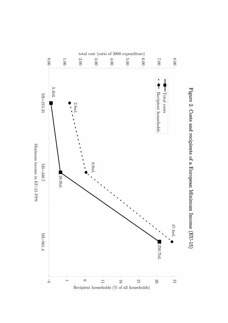
Figure 2. C
osts and recipients of a European M
inimum
Income (E
U-15)250.7bil.
28.9bil.
5.4bil.
47.4ml.
9.9ml.
2.8ml.
0.00
1.00
2.00
3.00
4.00
5.00
6.00
7.00
8.00
MI=
215.35M
I=430.7
MI=
861.4
Minim
um incom
e in EU
-15 PP
S
total cost (ratio of 2000 expenditure)
-4 1 6 11 16 21 26 31
Recipient households (% of all households)
Total costs
Recipient households

0.453
0.806
0.737
0.717
0.703
0.695
0.687
0.645
0.635
0.606
0.039
0.032
0.021
0.018
0.25
.5.75
1
EU
-13 .Finland
Denm
arkN
etherlandsA
ustriaIreland
Germ
anyU
nited Kingdom
BelgiumFrance
Greece
Portugal
ItalySpain
MI=
215.35
0.260
0.782
0.738
0.634
0.619
0.194
0.191
0.099
0.089
0.042
0.030
0.022
0.017
0.010
0.25
.5.75
1
EU
-13 .Finland
Denm
arkU
nited KingdomFrance
PortugalG
reeceSpainItaly
IrelandN
etherlandsA
ustriaG
ermany
Belgium
MI=
430.7
0.276
0.618
0.589
0.445
0.391
0.305
0.302
0.229
0.225
0.212
0.188
0.146
0.139
0.127
0.25
.5.75
1
EU
-13 .P
ortugalG
reeceSpainItaly
IrelandFinland
United K
ingdomFrance
Netherlands
Belgium
Austria
Germ
anyD
enmark
MI=
861.4
Autarky
0.661
0.797
0.749
0.739
0.717
0.712
0.709
0.701
0.687
0.643
0.641
0.631
0.604
0.552
0.25
.5.75
1
EU
-13 .Finland
Portugal
Denm
arkN
etherlandsA
ustriaIrelandSpain
Germ
anyItaly
Belgium
United K
ingdomFrance
Greece
MI=
215.35
0.052
0.194
0.191
0.099
0.089
0.042
0.034
0.030
0.029
0.025
0.022
0.017
0.011
0.010
0.25
.5.75
1
EU
-13 .P
ortugalG
reeceSpainItaly
IrelandU
nited Kingdom
Netherlands
FinlandFrance
Austria
Germ
anyD
enmark
Belgium
MI=
430.7
0.276
0.618
0.589
0.445
0.391
0.305
0.302
0.229
0.225
0.212
0.188
0.146
0.139
0.127
0.25
.5.75
1
EU
-13 .P
ortugalG
reeceSpainItaly
IrelandFinland
United K
ingdomFrance
Netherlands
Belgium
Austria
Germ
anyD
enmark
MI=
861.4
Centralised
Figure 3: F
raction of winners by country
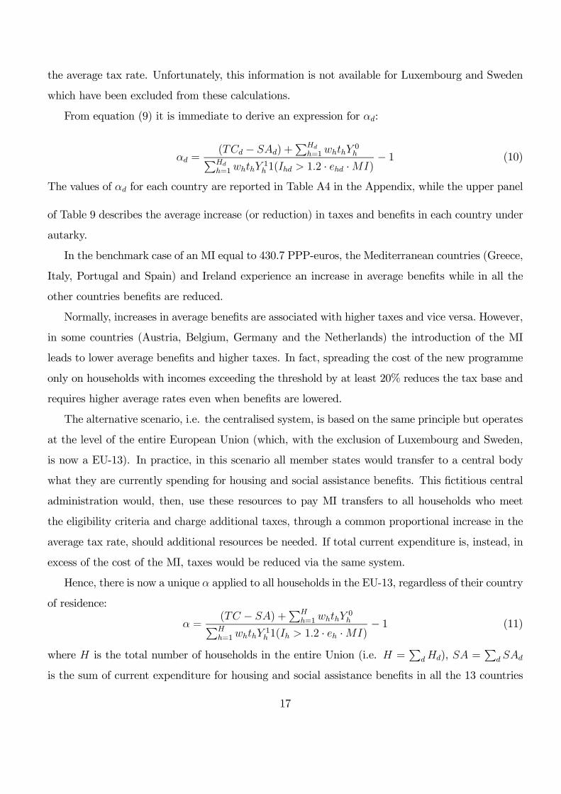
Stock of foregin population in 2001Country OECD1 ECHP2
Austria 9.40 6.48Belgium 8.21 8.63Denmark 5.00 3.46Finland 1.90 3.51France .. 7.52Germany 8.88 13.05Greece 7.00 4.41Ireland 3.90 3.73Italy 2.36 1.57Luxembourg 37.55 35.58Netherlands 4.26 1.61Portugal 2.17 2.47Spain 2.74 1.64Sweden 5.34 3.87United Kingdom 4.39 3.531. Source: Trends in International Migration, OECD, 2003 edition. Table A.1.52. Foreign population defined as persons who declare to be citizens of a foreign country or that they were born in a foreign country (or both)
Table 1. Comparison of data sources
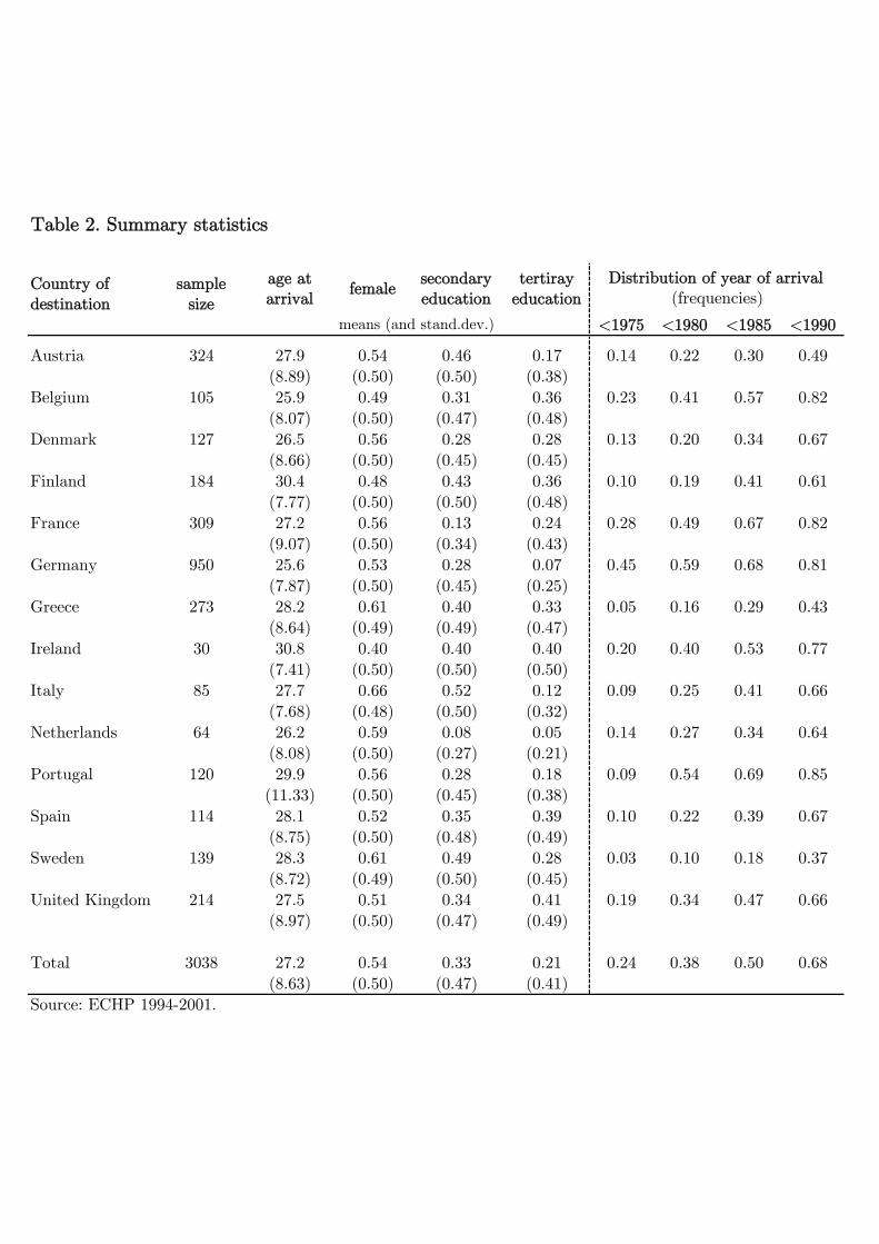
Table 2. Summary statistics
Country of destination
sample size
age at arrival
femalesecondary education
tertiray education
<1975 <1980 <1985 <1990
Austria 324 27.9 0.54 0.46 0.17 0.14 0.22 0.30 0.49(8.89) (0.50) (0.50) (0.38)
Belgium 105 25.9 0.49 0.31 0.36 0.23 0.41 0.57 0.82(8.07) (0.50) (0.47) (0.48)
Denmark 127 26.5 0.56 0.28 0.28 0.13 0.20 0.34 0.67(8.66) (0.50) (0.45) (0.45)
Finland 184 30.4 0.48 0.43 0.36 0.10 0.19 0.41 0.61(7.77) (0.50) (0.50) (0.48)
France 309 27.2 0.56 0.13 0.24 0.28 0.49 0.67 0.82(9.07) (0.50) (0.34) (0.43)
Germany 950 25.6 0.53 0.28 0.07 0.45 0.59 0.68 0.81(7.87) (0.50) (0.45) (0.25)
Greece 273 28.2 0.61 0.40 0.33 0.05 0.16 0.29 0.43(8.64) (0.49) (0.49) (0.47)
Ireland 30 30.8 0.40 0.40 0.40 0.20 0.40 0.53 0.77(7.41) (0.50) (0.50) (0.50)
Italy 85 27.7 0.66 0.52 0.12 0.09 0.25 0.41 0.66(7.68) (0.48) (0.50) (0.32)
Netherlands 64 26.2 0.59 0.08 0.05 0.14 0.27 0.34 0.64(8.08) (0.50) (0.27) (0.21)
Portugal 120 29.9 0.56 0.28 0.18 0.09 0.54 0.69 0.85(11.33) (0.50) (0.45) (0.38)
Spain 114 28.1 0.52 0.35 0.39 0.10 0.22 0.39 0.67(8.75) (0.50) (0.48) (0.49)
Sweden 139 28.3 0.61 0.49 0.28 0.03 0.10 0.18 0.37(8.72) (0.49) (0.50) (0.45)
United Kingdom 214 27.5 0.51 0.34 0.41 0.19 0.34 0.47 0.66(8.97) (0.50) (0.47) (0.49)
Total 3038 27.2 0.54 0.33 0.21 0.24 0.38 0.50 0.68(8.63) (0.50) (0.47) (0.41)
Source: ECHP 1994-2001.
Distribution of year of arrival (frequencies)
means (and stand.dev.)
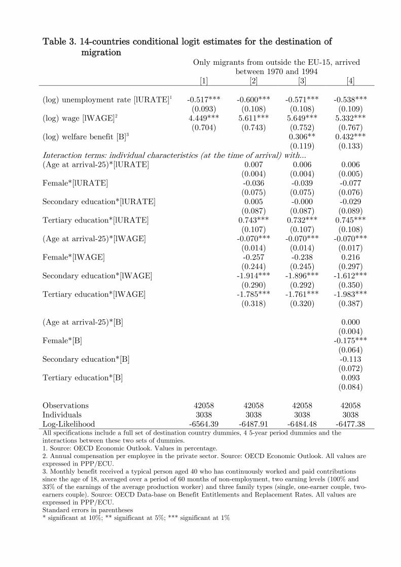
Table 3. 14-countries conditional logit estimates for the destination of migration
Only migrants from outside the EU-15, arrived between 1970 and 1994
[1] [2] [3] [4] (log) unemployment rate [lURATE]1 -0.517*** -0.600*** -0.571*** -0.538*** (0.093) (0.108) (0.108) (0.109) (log) wage [lWAGE]2 4.449*** 5.611*** 5.649*** 5.332*** (0.704) (0.743) (0.752) (0.767) (log) welfare benefit [B]3 0.306** 0.432*** (0.119) (0.133) Interaction terms: individual characteristics (at the time of arrival) with... (Age at arrival-25)*[lURATE] 0.007 0.006 0.006 (0.004) (0.004) (0.005) Female*[lURATE] -0.036 -0.039 -0.077 (0.075) (0.075) (0.076) Secondary education*[lURATE] 0.005 -0.000 -0.029 (0.087) (0.087) (0.089) Tertiary education*[lURATE] 0.743*** 0.732*** 0.745*** (0.107) (0.107) (0.108) (Age at arrival-25)*[lWAGE] -0.070*** -0.070*** -0.070*** (0.014) (0.014) (0.017) Female*[lWAGE] -0.257 -0.238 0.216 (0.244) (0.245) (0.297) Secondary education*[lWAGE] -1.914*** -1.896*** -1.612*** (0.290) (0.292) (0.350) Tertiary education*[lWAGE] -1.785*** -1.761*** -1.983*** (0.318) (0.320) (0.387)
(Age at arrival-25)*[B] 0.000 (0.004) Female*[B] -0.175*** (0.064) Secondary education*[B] -0.113 (0.072) Tertiary education*[B] 0.093 (0.084) Observations 42058 42058 42058 42058 Individuals 3038 3038 3038 3038 Log-Likelihood -6564.39 -6487.91 -6484.48 -6477.38 All specifications include a full set of destination country dummies, 4 5-year period dummies and the interactions between these two sets of dummies. 1. Source: OECD Economic Outlook. Values in percentage. 2. Annual compensation per employee in the private sector. Source: OECD Economic Outlook. All values are expressed in PPP/ECU. 3. Monthly benefit received a typical person aged 40 who has continuously worked and paid contributions since the age of 18, averaged over a period of 60 months of non-employment, two earning levels (100% and 33% of the earnings of the average production worker) and three family types (single, one-earner couple, two-earners couple). Source: OECD Data-base on Benefit Entitlements and Replacement Rates. All values are expressed in PPP/ECU. Standard errors in parentheses * significant at 10%; ** significant at 5%; *** significant at 1%
Countryown unemp. rate own wages own benefits
[1] [2] [3] [3]/[1] [3]/[2]
mean 6.7 18163.9 4986.0
std.dev. 3.1 3412.8 2993.7
Austria -0.0358 0.1067 0.0277 0.77 0.26Belgium -0.0112 0.0427 0.0071 0.64 0.17Denmark -0.0123 0.0537 0.0064 0.52 0.12Finland -0.0268 0.0717 0.0187 0.70 0.26France -0.0114 0.0619 0.0143 1.25 0.23Germany -0.0539 0.1549 0.0387 0.72 0.25Greece -0.0111 0.0633 0.0300 2.71 0.47Ireland -0.0015 0.0105 0.0030 1.96 0.29Italy -0.0041 0.0229 0.0239 5.88 1.04Netherlands -0.0107 0.0346 0.0054 0.50 0.16Portugal -0.0039 0.0227 0.0040 1.01 0.17Spain -0.0040 0.0342 0.0069 1.71 0.20Sweden -0.0275 0.0506 0.0099 0.36 0.20United Kingdom -0.0173 0.0631 0.0187 1.08 0.30
Average -0.0165 0.0567 0.0153 0.93 0.271. Male, aged 25, primary education, arrived in 1990.
Effect of an increase of 1 standard deviation in: Relative size of the own benefit effect
Table 4. Effects of one-standard deviation increases for the reference person 1
All effects are com
puted for the reference person1
Migration
probabilityabsolute change
Unem
ployment
ratechange (%
)A
nnual welfare
benefitschange (%
)
1. Benchm
ark
Country A
0.500-
6.0-
5000-
Country B
0.500-
6.0-
5000-
Country A
0.455-0.045
7.00.17
50000.00
Country B
0.5450.045
5.0-0.17
50000.00
Country A
0.5440.044
6.00.00
60000.20
Country B
0.456-0.044
6.00.00
4000-0.20
Country A
0.498-0.002
7.00.17
60000.20
Country B
0.5020.002
5.0-0.17
4000-0.20
1. Male, aged 25, prim
ary education, arrived in 1990.
2. Effect of increased dispersion in unem
ployment
3. Effect of increased dispersion in w
elfare
4. Cum
ulative effect of increased
Table 5. Sim
ulated effects of increased dispersion in unemploym
ent and welfare generosity
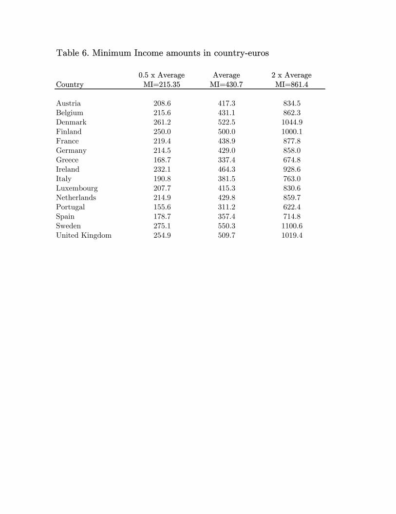
Table 6. Minimum Income amounts in country-euros
0.5 x Average Average 2 x AverageCountry MI=215.35 MI=430.7 MI=861.4
Austria 208.6 417.3 834.5Belgium 215.6 431.1 862.3Denmark 261.2 522.5 1044.9Finland 250.0 500.0 1000.1France 219.4 438.9 877.8Germany 214.5 429.0 858.0Greece 168.7 337.4 674.8Ireland 232.1 464.3 928.6Italy 190.8 381.5 763.0Luxembourg 207.7 415.3 830.6Netherlands 214.9 429.8 859.7Portugal 155.6 311.2 622.4Spain 178.7 357.4 714.8Sweden 275.1 550.3 1100.6United Kingdom 254.9 509.7 1019.4
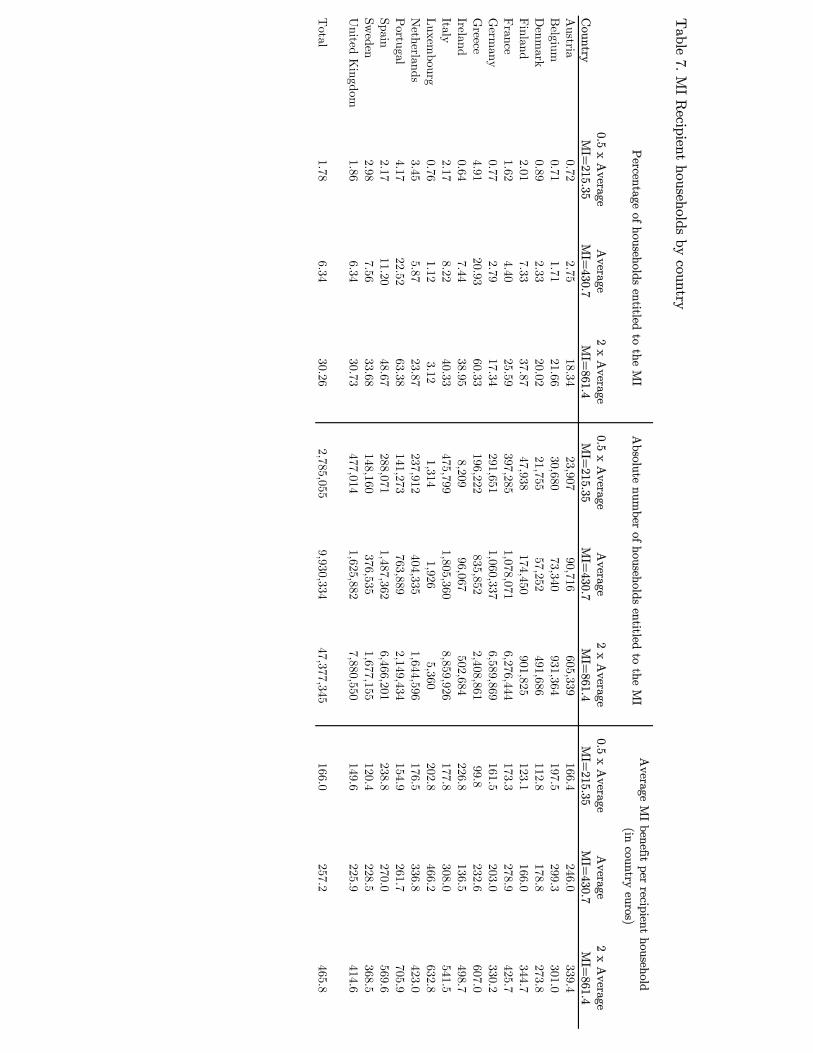
Table 7. M
I Recipient households by country
0.5 x Average
Average
2 x Average
0.5 x Average
Average
2 x Average
0.5 x Average
Average
2 x Average
Country
MI=
215.35M
I=430.7
MI=
861.4M
I=215.35
MI=
430.7M
I=861.4
MI=
215.35M
I=430.7
MI=
861.4A
ustria0.72
2.7518.34
23,90790,716
605,339166.4
246.0339.4
Belgium
0.711.71
21.6630,680
73,340931,364
197.5299.3
301.0D
enmark
0.892.33
20.0221,755
57,252491,686
112.8178.8
273.8Finland
2.017.33
37.8747,938
174,450901,825
123.1166.0
344.7France
1.624.40
25.59397,285
1,078,0716,276,444
173.3278.9
425.7G
ermany
0.772.79
17.34291,651
1,060,3376,589,869
161.5203.0
330.2G
reece4.91
20.9360.33
196,222835,852
2,408,86199.8
232.6607.0
Ireland0.64
7.4438.95
8,20996,067
502,684226.8
136.5498.7
Italy2.17
8.2240.33
475,7991,805,360
8,859,926177.8
308.0541.5
Luxem
bourg0.76
1.123.12
1,3141,926
5,360202.8
466.2632.8
Netherlands
3.455.87
23.87237,912
404,3351,644,596
176.5336.8
423.0P
ortugal4.17
22.5263.38
141,273763,889
2,149,434154.9
261.7705.9
Spain2.17
11.2048.67
288,0711,487,362
6,466,201238.8
270.0569.6
Sweden
2.987.56
33.68148,160
376,5351,677,155
120.4228.5
368.5U
nited Kingdom
1.866.34
30.73477,014
1,625,8827,880,550
149.6225.9
414.6
T
otal1.78
6.3430.26
2,785,0559,930,334
47,377,345166.0
257.2465.8
Percentage of households entitled to the M
IA
bsolute number of households entitled to the M
IA
verage MI benefit per recipient household
(in country euros)
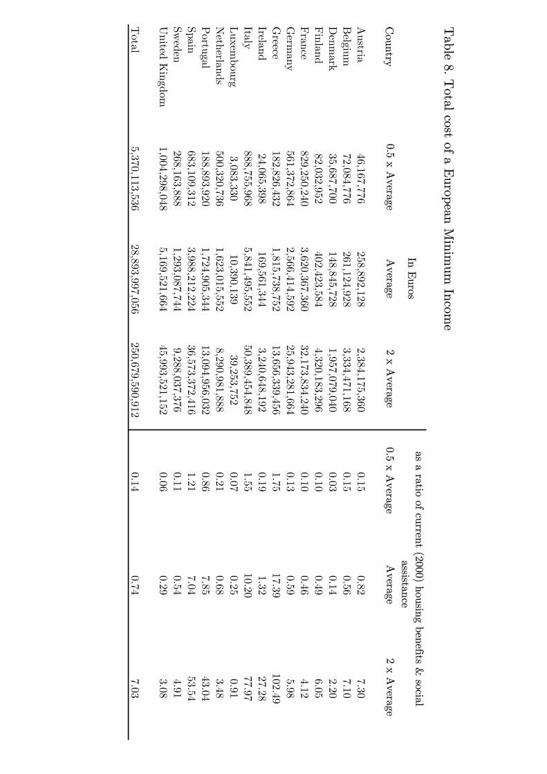
Table 8. T
otal cost of a European M
inimum
Income
In Euros
Country
0.5 x Average
Austria
46,167,776258,892,128
2,384,175,3600.15
0.827.30
Belgium
72,084,776261,124,928
3,334,471,1680.15
0.567.10
Denm
ark35,687,700
148,845,7281,957,079,040
0.030.14
2.20Finland
82,032,952402,423,584
4,320,183,2960.10
0.496.05
France
829,250,2403,620,367,360
32,173,834,2400.10
0.464.12
Germ
any561,372,864
2,566,414,59225,943,281,664
0.130.59
5.98G
reece182,826,432
1,815,738,75213,656,339,456
1.7517.39
102.49Ireland
24,065,398169,561,344
3,240,648,1920.19
1.3227.28
Italy888,755,968
5,841,495,55250,389,454,848
1.5510.20
77.97Luxem
bourg3,083,330
10,390,13939,253,752
0.070.25
0.91N
etherlands500,320,736
1,623,015,5528,290,981,888
0.210.68
3.48P
ortugal188,893,920
1,724,905,34413,094,956,032
0.867.85
43.04Spain
683,109,3123,988,212,224
36,573,372,4161.21
7.0453.54
Sweden
268,163,8881,293,087,744
9,288,037,3760.11
0.544.91
United K
ingdom1,004,298,048
5,169,521,66445,993,521,152
0.060.29
3.08
Total
5,370,113,53628,893,997,056
250,679,590,9120.14
0.747.03
Average
2 x Average
as a ratio of current (2000) housing benefits & social
assistance0.5 x A
verageA
verage2 x A
verage
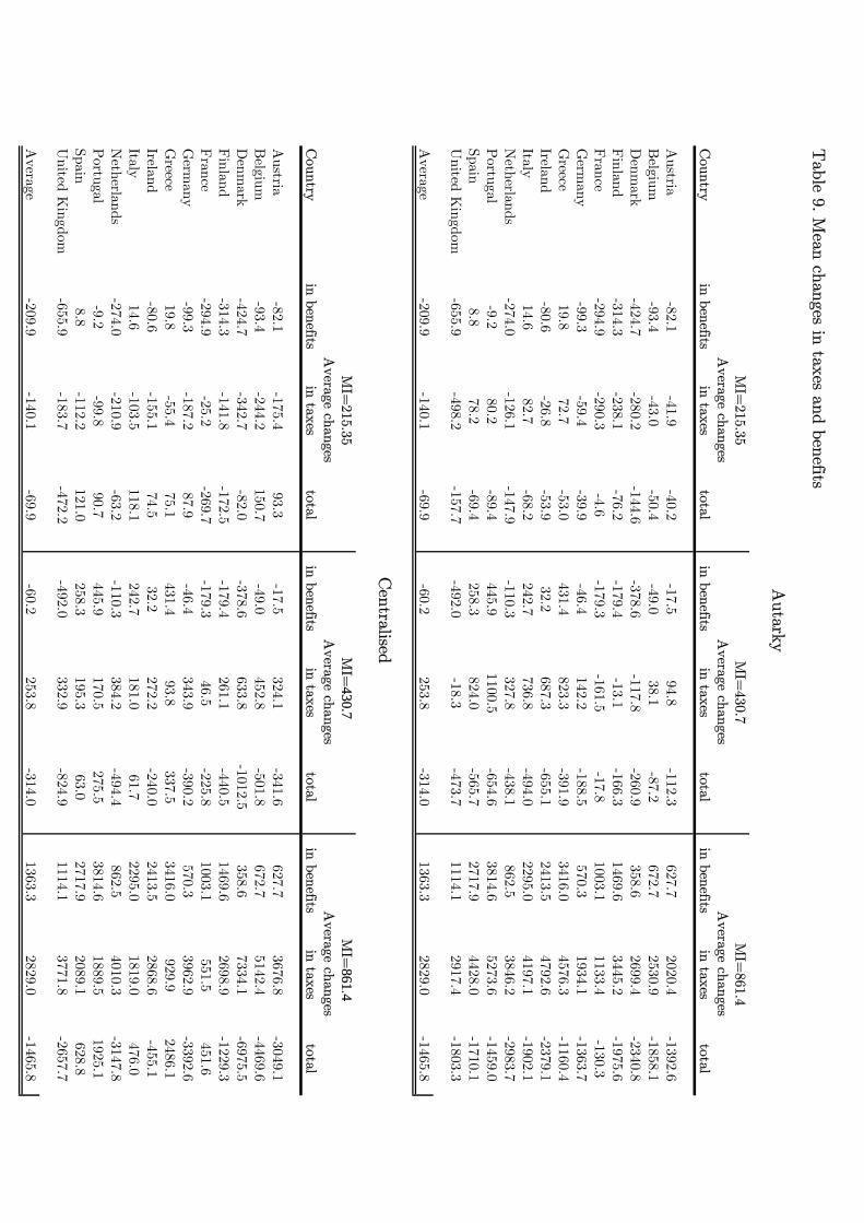
Table 9. M
ean changes in taxes and benefits
MI=
215.35M
I=430.7
MI=
861.4
Country
in benefitsin taxes
totalin benefits
in taxestotal
in benefitsin taxes
total
Austria
-82.1-41.9
-40.2-17.5
94.8-112.3
627.72020.4
-1392.6B
elgium-93.4
-43.0-50.4
-49.038.1
-87.2672.7
2530.9-1858.1
Denm
ark-424.7
-280.2-144.6
-378.6-117.8
-260.9358.6
2699.4-2340.8
Finland
-314.3-238.1
-76.2-179.4
-13.1-166.3
1469.63445.2
-1975.6France
-294.9-290.3
-4.6-179.3
-161.5-17.8
1003.11133.4
-130.3G
ermany
-99.3-59.4
-39.9-46.4
142.2-188.5
570.31934.1
-1363.7G
reece19.8
72.7-53.0
431.4823.3
-391.93416.0
4576.3-1160.4
Ireland-80.6
-26.8-53.9
32.2687.3
-655.12413.5
4792.6-2379.1
Italy14.6
82.7-68.2
242.7736.8
-494.02295.0
4197.1-1902.1
Netherlands
-274.0-126.1
-147.9-110.3
327.8-438.1
862.53846.2
-2983.7P
ortugal-9.2
80.2-89.4
445.91100.5
-654.63814.6
5273.6-1459.0
Spain8.8
78.2-69.4
258.3824.0
-565.72717.9
4428.0-1710.1
United K
ingdom-655.9
-498.2-157.7
-492.0-18.3
-473.71114.1
2917.4-1803.3
A
verage-209.9
-140.1-69.9
-60.2253.8
-314.01363.3
2829.0-1465.8
MI=
215.35M
I=430.7
MI=
861.4
Country
in benefitsin taxes
totalin benefits
in taxestotal
in benefitsin taxes
total
Austria
-82.1-175.4
93.3-17.5
324.1-341.6
627.73676.8
-3049.1B
elgium-93.4
-244.2150.7
-49.0452.8
-501.8672.7
5142.4-4469.6
Denm
ark-424.7
-342.7-82.0
-378.6633.8
-1012.5358.6
7334.1-6975.5
Finland
-314.3-141.8
-172.5-179.4
261.1-440.5
1469.62698.9
-1229.3France
-294.9-25.2
-269.7-179.3
46.5-225.8
1003.1551.5
451.6G
ermany
-99.3-187.2
87.9-46.4
343.9-390.2
570.33962.9
-3392.6G
reece19.8
-55.475.1
431.493.8
337.53416.0
929.92486.1
Ireland-80.6
-155.174.5
32.2272.2
-240.02413.5
2868.6-455.1
Italy14.6
-103.5118.1
242.7181.0
61.72295.0
1819.0476.0
Netherlands
-274.0-210.9
-63.2-110.3
384.2-494.4
862.54010.3
-3147.8P
ortugal-9.2
-99.890.7
445.9170.5
275.53814.6
1889.51925.1
Spain8.8
-112.2121.0
258.3195.3
63.02717.9
2089.1628.8
United K
ingdom-655.9
-183.7-472.2
-492.0332.9
-824.91114.1
3771.8-2657.7
A
verage-209.9
-140.1-69.9
-60.2253.8
-314.01363.3
2829.0-1465.8
Autarky
Average changes
Average changes
Average changes
Average changes
Average changes
Average changes
Centralised

Table A1. Robustness check Only migrants from outside the EU-15, arrived
between 1970 and 1994 [1] [2] [3] (log) unemployment rate [lURATE]1 -0.925*** -0.958*** -0.949*** (0.137) (0.151) (0.152) (log) wage [lWAGE]2 0.875 4.113*** 4.374*** (1.254) (1.340) (1.378) Public expenditure on unemployment related benefits (% of GDP) [B]3
0.354*** (0.134)
0.363*** (0.135)
0.312** (0.157)
Interaction terms: individual characteristics (at the time of arrival) with... (Age at arrival-25)*[lURATE] 0.005 0.004 (0.005) (0.005) Female*[lURATE] -0.155*** -0.163*** (0.032) (0.038) Secondary education*[lURATE] 0.008 0.014 (0.090) (0.091) Tertiary education*[lURATE] -0.153 -0.062 (0.538) (0.650) (Age at arrival-25)*[lWAGE] -0.042 -0.075 (0.105) (0.107) Female*[lWAGE] 0.745*** 0.739*** (0.134) (0.135) Secondary education*[lWAGE] -5.583*** -6.305*** (0.634) (0.765) Tertiary education*[lWAGE] -6.337*** -6.483*** (0.739) (0.890) (Age at arrival-25)*[B] 0.002 (0.006) Female*[B] -0.027 (0.093) Secondary education*[B] 0.187* (0.108) Tertiary education*[B] 0.029 (0.119) Observations 18882 18882 18882 Individuals 1683 1683 1683 Log-Likelihood -3140.257 -3053.4802 -3051.7642 All specifications include a full set of destination country dummies, 4 5-year period dummies and the interactions between these two sets of dummies. 1. Source: OECD Economic Outlook. Values in percentage. 2. Annual compensation per employee in the private sector. Source: OECD Economic Outlook. All values are expressed in PPP/ECU. 3. Source: Comparative Welfare State Dataset (2004) by Evelyne Huber, Charles Ragin, John D. Stephens, David Brady, and Jason Beckfield based on various OECD data sources. Standard errors in parentheses * significant at 10%; ** significant at 5%; *** significant at 1%
Unemployment rateAUT BEL DEN FIN FRA GER GRC IRL ITA NLD PRT ESP SWE UKG
AUT -3.577 0.162 0.180 0.398 0.169 0.989 0.161 0.021 0.057 0.154 0.054 0.057 0.396 0.257BEL 0.234 -1.117 0.074 0.164 0.070 0.408 0.066 0.009 0.024 0.064 0.022 0.024 0.164 0.106DEN 0.280 0.080 -1.226 0.197 0.084 0.489 0.080 0.011 0.028 0.076 0.027 0.028 0.196 0.127FIN 0.327 0.093 0.104 -2.680 0.098 0.570 0.093 0.012 0.033 0.089 0.031 0.033 0.229 0.148FRA 0.316 0.090 0.100 0.222 -1.142 0.551 0.090 0.012 0.032 0.086 0.030 0.032 0.221 0.144GER 1.055 0.301 0.335 0.741 0.315 -5.392 0.300 0.040 0.106 0.288 0.101 0.106 0.739 0.479GRC 0.246 0.070 0.078 0.173 0.074 0.430 -1.107 0.009 0.025 0.067 0.024 0.025 0.173 0.112IRL 0.055 0.016 0.017 0.039 0.016 0.096 0.016 -0.154 0.006 0.015 0.005 0.006 0.038 0.025ITA 0.109 0.031 0.035 0.077 0.033 0.191 0.031 0.004 -0.406 0.030 0.010 0.011 0.076 0.050NLD 0.207 0.059 0.066 0.145 0.062 0.361 0.059 0.008 0.021 -1.074 0.020 0.021 0.145 0.094PRT 0.062 0.018 0.020 0.043 0.018 0.108 0.018 0.002 0.006 0.017 -0.392 0.006 0.043 0.028ESP 0.135 0.039 0.043 0.095 0.040 0.236 0.038 0.005 0.014 0.037 0.013 -0.403 0.095 0.061SWE 0.210 0.060 0.067 0.148 0.063 0.367 0.060 0.008 0.021 0.057 0.020 0.021 -2.753 0.096UKG 0.341 0.097 0.108 0.239 0.102 0.595 0.097 0.013 0.034 0.093 0.033 0.034 0.238 -1.728
Average wagesAUT BEL DEN FIN FRA GER GRC IRL ITA NLD PRT ESP SWE UKG
AUT 10.675 -0.618 -0.787 -1.064 -0.916 -2.840 -0.919 -0.145 -0.321 -0.498 -0.315 -0.483 -0.729 -0.939BEL -0.698 4.266 -0.325 -0.439 -0.379 -1.173 -0.380 -0.060 -0.133 -0.206 -0.130 -0.200 -0.301 -0.388DEN -0.836 -0.306 5.368 -0.526 -0.453 -1.405 -0.455 -0.072 -0.159 -0.247 -0.156 -0.239 -0.360 -0.465FIN -0.975 -0.356 -0.454 7.168 -0.529 -1.638 -0.530 -0.084 -0.185 -0.287 -0.182 -0.279 -0.420 -0.542FRA -0.943 -0.345 -0.439 -0.593 6.193 -1.584 -0.513 -0.081 -0.179 -0.278 -0.176 -0.269 -0.406 -0.524GER -3.149 -1.151 -1.466 -1.981 -1.707 15.488 -1.713 -0.270 -0.598 -0.928 -0.588 -0.900 -1.357 -1.750GRC -0.735 -0.269 -0.342 -0.463 -0.399 -1.236 6.326 -0.063 -0.140 -0.217 -0.137 -0.210 -0.317 -0.409IRL -0.164 -0.060 -0.076 -0.103 -0.089 -0.275 -0.089 1.046 -0.031 -0.048 -0.031 -0.047 -0.071 -0.091ITA -0.326 -0.119 -0.152 -0.205 -0.177 -0.548 -0.177 -0.028 2.286 -0.096 -0.061 -0.093 -0.141 -0.181NLD -0.617 -0.226 -0.287 -0.388 -0.335 -1.037 -0.336 -0.053 -0.117 3.463 -0.115 -0.176 -0.266 -0.343PRT -0.185 -0.067 -0.086 -0.116 -0.100 -0.310 -0.100 -0.016 -0.035 -0.054 2.274 -0.053 -0.080 -0.103ESP -0.403 -0.147 -0.188 -0.254 -0.219 -0.678 -0.219 -0.035 -0.077 -0.119 -0.075 3.419 -0.174 -0.224SWE -0.628 -0.230 -0.292 -0.395 -0.341 -1.056 -0.342 -0.054 -0.119 -0.185 -0.117 -0.180 5.059 -0.349UKG -1.016 -0.372 -0.473 -0.640 -0.551 -1.708 -0.553 -0.087 -0.193 -0.300 -0.190 -0.291 -0.438 6.308
Welfare benefitsAUT BEL DEN FIN FRA GER GRC IRL ITA NLD PRT ESP SWE UKG
AUT 2.772 -0.103 -0.094 -0.277 -0.211 -0.710 -0.435 -0.042 -0.335 -0.078 -0.055 -0.097 -0.142 -0.278BEL -0.181 0.712 -0.039 -0.115 -0.087 -0.293 -0.180 -0.017 -0.138 -0.032 -0.023 -0.040 -0.059 -0.115DEN -0.217 -0.051 0.640 -0.137 -0.105 -0.351 -0.215 -0.021 -0.166 -0.039 -0.027 -0.048 -0.070 -0.138FIN -0.253 -0.059 -0.054 1.870 -0.122 -0.410 -0.251 -0.024 -0.193 -0.045 -0.032 -0.056 -0.082 -0.160FRA -0.245 -0.058 -0.052 -0.155 1.428 -0.396 -0.243 -0.023 -0.187 -0.043 -0.031 -0.054 -0.079 -0.155GER -0.818 -0.192 -0.175 -0.517 -0.394 3.873 -0.811 -0.078 -0.624 -0.145 -0.103 -0.181 -0.265 -0.518GRC -0.191 -0.045 -0.041 -0.121 -0.092 -0.309 2.996 -0.018 -0.146 -0.034 -0.024 -0.042 -0.062 -0.121IRL -0.042 -0.010 -0.009 -0.027 -0.020 -0.069 -0.042 0.301 -0.032 -0.008 -0.005 -0.009 -0.014 -0.027ITA -0.085 -0.020 -0.018 -0.054 -0.041 -0.137 -0.084 -0.008 2.388 -0.015 -0.011 -0.019 -0.027 -0.054NLD -0.160 -0.038 -0.034 -0.101 -0.077 -0.259 -0.159 -0.015 -0.122 0.542 -0.020 -0.036 -0.052 -0.101PRT -0.048 -0.011 -0.010 -0.030 -0.023 -0.078 -0.048 -0.005 -0.037 -0.009 0.397 -0.011 -0.016 -0.030ESP -0.105 -0.025 -0.022 -0.066 -0.050 -0.169 -0.104 -0.010 -0.080 -0.019 -0.013 0.689 -0.034 -0.066SWE -0.163 -0.038 -0.035 -0.103 -0.079 -0.264 -0.162 -0.016 -0.125 -0.029 -0.020 -0.036 0.987 -0.103UKG -0.264 -0.062 -0.056 -0.167 -0.127 -0.427 -0.262 -0.025 -0.202 -0.047 -0.033 -0.059 -0.086 1.8661. Male, aged 25, primary education, arrived in 1990.
(all effects are multiplied by 100)Table A2. Cross-effects of one-standard deviation increases for the reference person1
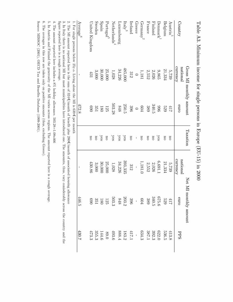
Table A
3. Minim
um incom
e for single persons in Europe (E
U-15) in 2000
Taxation
Country
national currency
euronational currency
euroP
PS
Austria
55,739
417no
5,739417
413.8B
elgium21,334
529no
21,334529
536.5
Denm
ark1
9,865996
yes6,691.1
675.6622.0
Finland
2,026340.5
no2,026
340.5392.3
France
2,552389
no2,552
389387.1
Germ
any2
1,181604
no1,181.0
604634.3
Greece
00
--
--
Ireland312
396no
312396
417.1
Italy3
485,000250.5
yes393,335
203.2183.2
Luxem
bourg34,226
848yes
34,226848
888.4
Netherlands
41,028
503.28yes
1,028503.3
493.6
Portugal 5
25,000125
no25,000
12589.0
Spain30,000
180yes
30,000180
144.6Sw
eden3,000
351no
3,000351
355.3U
nited Kingdom
431690
no430.86
690473.3
Average
6-
472.8-
446.5430.7
1. For single persons below
25y.o. Living alone the M
I is 639€ per m
onth
4. The am
ount reported here includes a 8% holiday allow
ance. 503.28=1.08x466
5. In Austria and F
inland the generosity of the MI varies across regions. T
he amount reported here is a rough average.
6. The averages in this row
are taken only on positive smounts (thus, excluding G
reece).
Source: MISSO
C (2001), O
EC
D T
ax and Benefits D
atabase (1999-2001).
3. In Italy there is no national MI but m
ost municipalities have introduced one. T
he amounts, thus, vary conisderably across the country and the
figure reported here is a rough average.
Gross M
I monthly am
ountN
et MI m
onthly amount
2. The M
I amount reported here is the sum
of 324€/m
onth of benefit plus 280€/month of associated housing allow
ance
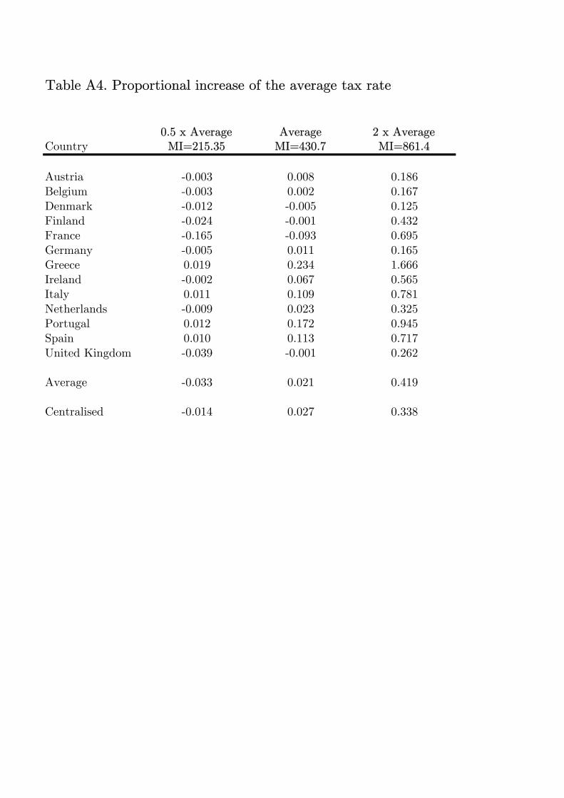
0.5 x Average Average 2 x AverageCountry MI=215.35 MI=430.7 MI=861.4
Austria -0.003 0.008 0.186Belgium -0.003 0.002 0.167Denmark -0.012 -0.005 0.125Finland -0.024 -0.001 0.432France -0.165 -0.093 0.695Germany -0.005 0.011 0.165Greece 0.019 0.234 1.666Ireland -0.002 0.067 0.565Italy 0.011 0.109 0.781Netherlands -0.009 0.023 0.325Portugal 0.012 0.172 0.945Spain 0.010 0.113 0.717United Kingdom -0.039 -0.001 0.262
Average -0.033 0.021 0.419
Centralised -0.014 0.027 0.338
Table A4. Proportional increase of the average tax rate