weil representation, deligne sheaf and proof of the ... · weil representation, deligne sheaf and...
TRANSCRIPT
arX
iv:m
ath-
ph/0
6010
31v1
15
Jan
2006
Weil Representation, Deligne Sheaf and
Proof of the Kurlberg-Rudnick
Conjecture
Thesis submitted for the degree “Doctor of Philosophy”
by
Shamgar Gurevich
Prepared under the supervision of
Professor Joseph Bernstein
Presented to the Tel-Aviv University Senate
March 2005
arX
iv:m
ath-
ph/0
6010
31v1
15
Jan
2006
This Ph.D. thesis was written under the supervision of
Prof. Joseph Bernstein
arX
iv:m
ath-
ph/0
6010
31v1
15
Jan
2006
Acknowledgements
This work is for me a conclusion of four years of activity in a research project under thedirection of prof. Joseph Bernstein. I would like to use this opportunity to thank himsincerely for letting me join this intellectual voyage and having thought me as much asthe little that I know. Working with Joseph and learning from him is an experience thatI will cherish for all my life.
Large parts of this work are a result of a joint project with my friend Ronny Hadani.I thank him and share my deep appreciation for the long way we walked side by side andthe thousands of hours we spent working together here in Israel and far abroad the states.
This thesis stands across the fine bridge between mathematics and physics. This is afascinating and exotic domain of knowledge, which spreads its roots into multiple areas ofresearch. I owe a great deal to Dr. Par Kurlberg and Prof. Zeev Rudnick for explainingme their ideas about ”Quantum Chaos”. I would like to thank Prof. David Kazhdan forsharing his thoughts about the possible existence of canonical Hilbert spaces. In additionI thank Prof. Peter Sarnak for some interesting discussions. Finally, I would like to thankProf. Pierre Deligne for letting me use his ideas about the geometrization of the Weilrepresentation which appeared in a letter he wrote to David Kazhdan in 1982.
In the course of my work I had the privilege to visit and to give lectures in severalinstitutions around the world. I would like to thank them for their hospitality and forproviding me with excellent working conditions. In this list I count: MSRI, Berkeley Uni-versity, IHES, Gothenburg University, Max-Planck Institute at Bonn, Bonn University,Courant Institute, Princeton University, Yale University and Ohio state University.
I am happy to have the opportunity to thank my friends: S. Artstein, D. Blanck, D.Gaitsgory, Y. Ostrover, Y. Kremnizer, D. Mangobi, Y. Peterzil, N. Porat, E. Sayag, I.Tyomkin and D. Yekutieli who supported me, each of them in his own special way.
Finally, I would like to thank my family: my parents Noga and Oded and my broth-ers Navot, Hamutal and Ira.
i

ii
Abstract
Consider the two dimensional symplectic torus (T, ω) and an hyperbolic automorphismA of T. The automorphism A is known to be ergodic. In 1980, using a non-trivial pro-cedure called quantization, the physicists J. Hannay and M.V. Berry attached to thisautomorphism a quantum operator ρ
~(A) acting on a Hilbert space H~. One of the cen-
tral questions of ”Quantum Chaos Theory”, in this model, is whether the operator ρ~(A)
is ”quantum ergodic”?
We consider the following two distributions on the algebra A = C∞(T) of smooth complexvalued functions on T. The first one is given by the Haar integral:
f 7−→∫
T
fω
and the second one is given by the Wigner distribution:
f 7−→ Wχ(f)
defined as the expectation of the ”quantum observable” π~(f) in the Hecke state vχ, i.e.
Wχ(f) := 〈vχ|π~(f)vχ〉. Here the vector vχ is a common eigenvector, with eigencharacter
χ, of the Hecke group of symmetries of the quantum operator ρ~(A).
The Kurlberg-Rudnick rate conjecture is a quantitative description of the behavior of theWigner distribution attached to the ergodic automorphism A. It states that for Planckconstant of the form ~ = 1
p, where p is a prime number, one has:
Rate Conjecture. The following bound holds:∣
∣
∣
∣
Wχ(f)−∫
T
fω
∣
∣
∣
∣
≤ Cf√p
where Cf is a constant that depends only on the function f .
In the current thesis we present a proof of the Kurlberg-Rudnick conjecture. This is
iii
iv
carried out using new representation theoretic constructions and algebro-geometric sheafrealization of the Weil metaplectic representation, which was proposed by P. Deligne in1982.
Contents
Abstract iii
Introduction 1
1 The Hannay-Berry Model 9
1.1 Classical Torus . . . . . . . . . . . . . . . . . . . . . . . . . . . . . . . . . 9
1.1.1 Classical mechanical system . . . . . . . . . . . . . . . . . . . . . . 9
1.2 Quantization of the Torus . . . . . . . . . . . . . . . . . . . . . . . . . . . 10
1.2.1 The Weyl quantization model . . . . . . . . . . . . . . . . . . . . . 11
1.2.2 Equivariant Weyl quantization of the torus . . . . . . . . . . . . . . 12
1.2.3 Quantum mechanical system . . . . . . . . . . . . . . . . . . . . . . 14
2 The Kurlberg-Rudnick Conjecture 15
2.1 Hecke Quantum Unique Ergodicity . . . . . . . . . . . . . . . . . . . . . . 15
2.1.1 Formulation of the Kurlberg-Rudnick conjecture . . . . . . . . . . . 16
2.2 Proof of the Kurlberg-Rudnick conjecture . . . . . . . . . . . . . . . . . . 16
2.2.1 Preparation stage . . . . . . . . . . . . . . . . . . . . . . . . . . . . 16
2.2.2 The trace function . . . . . . . . . . . . . . . . . . . . . . . . . . . 18
2.2.3 Geometrization (Sheafification) . . . . . . . . . . . . . . . . . . . . 19
2.2.4 Geometric statement . . . . . . . . . . . . . . . . . . . . . . . . . . 23
2.2.5 Proof of the Vanishing Lemma . . . . . . . . . . . . . . . . . . . . . 25
3 Metaplectique 27
v
vi CONTENTS
3.1 Canonical Hilbert space . . . . . . . . . . . . . . . . . . . . . . . . . . . . 28
3.1.1 Oriented Lagrangian subspace . . . . . . . . . . . . . . . . . . . . . 28
3.1.2 The Heisenberg group . . . . . . . . . . . . . . . . . . . . . . . . . 28
3.1.3 Models of irreducible representation . . . . . . . . . . . . . . . . . . 28
3.1.4 Canonical intertwining operators . . . . . . . . . . . . . . . . . . . 29
3.1.5 Canonical Hilbert space . . . . . . . . . . . . . . . . . . . . . . . . 30
3.2 The Weil representation . . . . . . . . . . . . . . . . . . . . . . . . . . . . 30
3.3 Realization and formulas . . . . . . . . . . . . . . . . . . . . . . . . . . . . 31
3.3.1 Schrodinger realization . . . . . . . . . . . . . . . . . . . . . . . . . 31
3.3.2 Formulas for the Weil representation . . . . . . . . . . . . . . . . . 31
3.3.3 Formulas for the Heisenberg representation . . . . . . . . . . . . . . 32
3.3.4 Formulas for the representation of the semi-direct product . . . . . 33
3.4 Deligne’s letter . . . . . . . . . . . . . . . . . . . . . . . . . . . . . . . . . 33
3.4.1 Uniqueness and existence of the Weil representation sheaf . . . . . . 34
3.5 Proofs . . . . . . . . . . . . . . . . . . . . . . . . . . . . . . . . . . . . . . 37
4 The Two Dimensional Hannay-Berry Model 48
4.1 Introduction . . . . . . . . . . . . . . . . . . . . . . . . . . . . . . . . . . . 48
4.1.1 Motivation . . . . . . . . . . . . . . . . . . . . . . . . . . . . . . . . 48
4.1.2 Results . . . . . . . . . . . . . . . . . . . . . . . . . . . . . . . . . . 49
4.2 Construction . . . . . . . . . . . . . . . . . . . . . . . . . . . . . . . . . . 51
4.2.1 The quantum tori . . . . . . . . . . . . . . . . . . . . . . . . . . . . 52
4.2.2 Weyl quantization . . . . . . . . . . . . . . . . . . . . . . . . . . . . 52
4.2.3 Projective equivariant quantization . . . . . . . . . . . . . . . . . . 52
4.2.4 The canonical equivariant quantization . . . . . . . . . . . . . . . . 53
4.2.5 Unitary structure . . . . . . . . . . . . . . . . . . . . . . . . . . . . 53
4.3 Proofs . . . . . . . . . . . . . . . . . . . . . . . . . . . . . . . . . . . . . . 53
4.3.1 Proof of Lemma 4.2.1 . . . . . . . . . . . . . . . . . . . . . . . . . . 53
4.3.2 Proof of Proposition 4.2.2 . . . . . . . . . . . . . . . . . . . . . . . 54
CONTENTS vii
4.3.3 Proof of Theorem 4.1.5 . . . . . . . . . . . . . . . . . . . . . . . . . 55
Appendices 56
A The Higher Dimensional Hannay-Berry Model 56
A.1 Introduction . . . . . . . . . . . . . . . . . . . . . . . . . . . . . . . . . . . 56
A.1.1 Motivation . . . . . . . . . . . . . . . . . . . . . . . . . . . . . . . . 56
A.1.2 Definitions . . . . . . . . . . . . . . . . . . . . . . . . . . . . . . . . 57
A.1.3 Results . . . . . . . . . . . . . . . . . . . . . . . . . . . . . . . . . . 58
A.2 Construction . . . . . . . . . . . . . . . . . . . . . . . . . . . . . . . . . . 59
A.2.1 The quantum tori . . . . . . . . . . . . . . . . . . . . . . . . . . . . 59
A.2.2 Weyl quantization . . . . . . . . . . . . . . . . . . . . . . . . . . . . 59
A.2.3 Equivariant quantization . . . . . . . . . . . . . . . . . . . . . . . . 60
A.2.4 The equivariant quantization . . . . . . . . . . . . . . . . . . . . . . 60
A.2.5 Unitary structure . . . . . . . . . . . . . . . . . . . . . . . . . . . . 60
A.3 Proofs . . . . . . . . . . . . . . . . . . . . . . . . . . . . . . . . . . . . . . 61
A.3.1 Proof of Lemma A.2.1 . . . . . . . . . . . . . . . . . . . . . . . . . 61
A.3.2 Proof of Proposition A.2.2 . . . . . . . . . . . . . . . . . . . . . . . 61
B Two higher-dimensional (counter) examples 63
C Proofs for Chapters 1 and 2 65
C.1 Proof of Theorem 1.2.2 . . . . . . . . . . . . . . . . . . . . . . . . . . . . . 65
C.2 Proof of Lemma 2.2.3 . . . . . . . . . . . . . . . . . . . . . . . . . . . . . . 68
C.3 Proof of the Geometrization Theorem . . . . . . . . . . . . . . . . . . . . . 69
C.4 Computations for the Vanishing Lemma . . . . . . . . . . . . . . . . . . . 71
Bibliography 74

viii CONTENTS
Introduction
Hannay-Berry model
In the paper “Quantization of linear maps on the torus - Fresnel diffraction by a periodic
grating”, published in 1980 [HB], the physicists and J. Hannay and M.V. Berry explore amodel for quantum mechanics on the two dimensional symplectic torus (T, ω). Hannayand Berry suggested to quantize simultaneously the functions on the torus and the linearsymplectic group Γ = SL2(Z).
Quantum chaos
One of their main motivations was to study the phenomenon of quantum chaos [R2, S2]in this model. More precisely, they considered an ergodic discrete dynamical system onthe torus, which is generated by an hyperbolic automorphism A ∈ SL2(Z). Quantizingthe system, we replace: the classical phase space (T, ω) by a Hilbert space H~, classicalobservables, i.e., functions f ∈ C∞(T), by operators π
~(f) ∈ End(H~) and classical
symmetries by a unitary representation ρ~: SL2(Z) −→ U(H~). A fundamental meta-
question in the area of quantum chaos is to understand the ergodic properties of thequantum system ρ
~(A), at least in the semi-classical limit as ~→ 0.
Hecke quantum unique ergodicity
This question was addressed in a paper by Kurlberg and Rudnick [KR1]. In this paper theyformulated a rigorous definition of quantum ergodicity for the case ~ = 1
p. The following
is a brief description of that work. The basic observation is that the representation ρ~
factors through the quotient group Γp ⋍ SL2(Fp). We denote by TA ⊂ Γp the centralizerof the element A, now considered as an element of the quotient group Γp. The group TAis called (cf. [KR1]) the Hecke torus corresponding to the element A. The Hecke torus
1
2 INTRODUCTION
acts semisimply on H~. Therefore we have a decomposition:
H~ =⊕
χ:TA−→C∗
Hχ
where Hχ is the Hecke eigenspace corresponding to the character χ. Considering a unitvector v ∈ Hχ, one defines the Wigner distribution Wχ : C∞(T) −→ C by the formulaWχ(f) := 〈v|π~
(f)v〉. The main statement in [KR1] asserts about an explicit bound ofthe semi-classical asymptotic of Wχ(f):
∣
∣
∣
∣
Wχ(f)−∫
T
fω
∣
∣
∣
∣
≤ Cfp1/4
where Cf is a constant that depends only on the function f . In Rudnick’s lectures atMSRI, Berkeley 1999 [R1] and ECM, Barcelona 2000 [R2] he conjectured that a strongerbound should hold true, namely:
Conjecture (Rate Conjecture). The following bound holds:∣
∣
∣
∣
Wχ(f)−∫
T
fω
∣
∣
∣
∣
≤ Cfp1/2
.
The basic clues suggesting the validity of this stronger bound come from two mainsources. The first source is computer simulations [Ku] accomplished over the years togive extremely precise bounds for considerably large values of p. A more mathematicalargument is based on the fact that for special values of p, in which the Hecke torus splits,namely TA ≃ F∗
p, one is able to compute explicitly the eigenvector v ∈ Hχ and as aconsequence to give an explicit formula for the Wigner distribution [KR2, DGI]. Moreprecisely, in case ξ ∈ T∨ , i.e., a character, the distribution Wχ(ξ) turns out to be equalto an exponential sum very much similar to the Kloosterman sum:
1
p
∑
a∈F∗p
ψ
(
a+ 1
a− 1
)
σ(a)χ(a)
where σ denotes the Legendre character. In this case the classical Weil bound [W1]yields the result. In this thesis a proof of the rate conjecture, for all tori (split or inert)simultaneously, is presented. For this peropus we view things from a more abstractperspective.
Geometric approach (Deligne sheaf)
The basic observation to be made is that the theory of quantum mechanics on the torus,in case ~ = 1
p, can be equivalently recast in the language of representation theory of finite
INTRODUCTION 3
groups in characteristic p. We will endeavor to give a more precise explanation of thismatter. Consider the quotient Fp-vector space V = T∨/pT∨, where T∨ is the lattice ofcharacters on T. We denote by E = E(V) the Heisenberg group. The group Γp ⋍ SL2(Fp)is naturally identified with the group of linear symplectomorphisms of V. We have anaction of Γp on E. The Stone-von Neumann theorem states that there exists a uniqueirreducible representation π : E −→ GL(H), with the non-trivial central character ψ,for which its isomorphism class is fixed by Γp. This is equivalent to saying that H isequipped with a compatible projective representation ρ : Γp −→ PGL(H). Noting that Eand Γp are the sets of rational points of corresponding algebraic groups, it is natural toask whether there exists an algebro-geometric object that underlies the pair (π, ρ)?. Theanswer to this question is positive. The construction is proposed in an unpublished letterthat was sent in 1982 from Pierre Deligne to David Kazhdan [D1]. Parts of this letter willbe published for the first time in this thesis. In one sentence, the content of this letter isa construction of Representation Sheaves Kπ and Kρ on the algebraic varieties E and SL2
respectively. One obtains, as a consequence, the following general principle:
(*) Motivic principle. All quantum mechanical quantities in the Hannay-Berry modelare motivic in nature.
By this we mean that every quantum-mechanical quantity Q, is associated with a vectorspace VQ endowed with a Frobenius action Fr : VQ −→ VQ s.t.:
Q = Tr(Fr|VQ).
The main contribution of this paper is to implement this principle. In particular we showthat there exists a two dimensional vector space Vχ, endowed with an action Fr : Vχ −→Vχ s.t.:
Wχ(ξ) = Tr(Fr|Vχ).
This, combined with a bound on the modulus of the eigenvalues of Frobenius, i.e.,
∣
∣
∣e.v(Fr|Vχ
)∣
∣
∣≤ 1
p1/2,
completes the proof of the rate conjecture.
Side remarks
There are two remarks we would like to make at this point:
4 INTRODUCTION
Remark 1: Discreteness principle. “Every” quantity Q that appears in the Hannay-Berry model admits discrete spectrum in the following arithmetic sense: the modulus |Q|can take only values of the form pi/2 for i ∈ Z. This is a consequence of principle (*)and Deligne’s weight theory [D2]. We believe that this principle can be effectively usedin various situations in order to derive strong bounds out of weaker bounds. A striking
example is an alternative trivial ”proof” for the bound |Wχ(ξ)| ≤ Cξ
p1/2:
|Wχ(ξ)| ≤Cξp1/4
⇒ |Wχ(ξ)| ≤Cξp1/2
.
Kurlberg and Rudnick proved in their paper [KR1] the weak bound |Wχ(ξ)| ≤ Cξ
p1/4. This
directly implies (under certain mild assumptions) that the stronger bound |Wχ(ξ)| ≤ Cξ
p1/2
is valid.
Remark 2: Higher dimensional exponential sums. Proving the bound |Wχ(f)| ≤Cf√pcan be equivalently stated as bounding by
Cf√pthe spectral radius of the operator
AvTA(f) := 1
|TA|∑
B∈TA
ρ~(B)π
~(f)ρ
~(B−1). This implies a bound on the LN norms, for
every N ∈ Z+:
‖AvTA(f)‖N ≤
CfpN. (1)
In particular for 0 6= f = ξ ∈ T∨ one can compute explicitly the left hand side of (1) andobtain:
‖AvTA(ξ)‖N := Tr(|AvTA
(ξ)|N) = 1
|TA|2N∑
(x1,...,x2N )∈Xψ(
∑
i<j
ω(xi, xj))
where X := {(x1, . . . , x2N)| xi ∈ Oξ,∑
xi = 0} and Oξ := TA ·ξ ⊂ V denotes the orbit ofξ under the action of TA. Therefore referring to (1) we obtained a non-trivial bound for ahigher dimensional exponential sum. It would be interesting to know whether there existsan independent proof for this bound and whether this representation theoretic approachcan be used to prove optimal bounds for other interesting higher dimensional exponentialsums.
Sato-Tate conjecture
The next level of the theory is to understand the complete statistics of the Hecke-Wignerdistributions for different Hecke states. More precisely, let us fix a character ξ ∈ T∨. Forevery character χ : TA −→ C∗ we consider the normalized value Wχ(ξ) := 1
2√pWχ(ξ),
INTRODUCTION 5
which lies in the interval [−1, 1]. Now running over all multiplicative characters we definethe following atomic measure on the interval [−1, 1]:
µp :=1
|TA|∑
χ
δWχ(ξ).
One would like to describe the limit measure (if it exists!). This is the content of anotherconjecture of Kurlberg and Rudnick [KR2]:
Conjecture (Sato-Tate Conjecture). The following limit exists:
limp→∞
µp = µST
where µST is the projection of the Haar measure on S1 to the interval [−1, 1].
We hope that by using the methodology described in this paper one will be able togain some progress in proving this conjecture.
Remark. Note that the family {Wχ(ξ)}χ∈T∗Aruns over a non-algebraic space of pa-
rameters. Hence Deligne’s equidistribution theory (cf. Weil II [D2]) can not be applieddirectly in order to solve the Sato-Tate Conjecture.
Results
1. Kurlberg-Rudnick conjecture. The main result of the current work is Theorem2.1.1, which is the proof of the Kurlberg-Rudnick rate conjecture on the asymptoticbehavior of the Hecke-Wigner distributions.
2. Weil representation and the Hannay-Berry model. We introduce two new
constructions of the Weil representation over Z and over the finite fields Fq ofcharacteristic 6= 2. As an application we obtained a construction of the Hannay-Berry model.
(a) The first construction is stated in Theorem 1.2.2, Corollary 4.1.4 and Corol-lary A.1.2. It is based on the Rieffel quantum torus A~, for ~ ∈ Q. Thisapproach is essentially equivalent to the classical approach (cf. [Kl, W2]) thatuses the representation theory of the Heisenberg group in characteristic p. Asan application we obtained (Chapters 1, 4 and Appendix A) a constructionof the Hannay-Berry model of quantum mechanics for Tori in all dimensions.This is a new realization of the Hannay-Berry model. This was an important
6 INTRODUCTION
achievement, since the original Hannay-Berry model was formulated in phys-ical terms. In particular, using this new approach we were able to construct(Chapters 1 and 4) a slightly more general model which has a larger and al-gebraic group of symmetries, namely the whole symplectic group Γ = SL2(Z).This was then generalized (Appendix A) to the higher dimensional tori andthe groups Sp(2n,Z).
(b) Canonical Hilbert space (Kazhdan’s question). The second construc-tion uses our new ”Method of Canonical Hilbert Space” (see Chapter 3). Thisapproach is based on the following statement:
Proposition (Canonical Hilbert Space). Let (V, ω) be a two dimensionalsymplectic vector space over the finite field Fq. There exists a canonical Hilbertspace HV attached to V.
An immediate consequence of this proposition is that all symmetries of (V, ω)automatically act on HV. In particular, we obtain a linear representation ofthe group Spω := Spω(V, ω) on HV. Probably this approach has higher dimen-sional generalization, for the case where V is of dimension 2n. This will be asubject of a future publication.
Remark. Note the main difference of our construction from the classicalapproach due to Weil (cf. [W2]). The classical construction proceeds in twostages. Firstly, one obtains a projective representation of Spω and secondlyusing general arguments about the group Spω, one proves the existence of a lin-earization. A consequence of our approach is that there exists a distinguished
linear representation and its existence is not related to any group theoreticproperty of Spω. We would like to mention that this approach answers, in thecase of the two dimensional Heisenberg group, a question of David Kazhdan
[Ka] dealing with the existence of Canonical Hilbert Spaces for co-adjoint or-bits of general unipotent groups. The main motive behind our construction isthe notion of oriented Lagrangian subspace. This idea was suggested to us byJoseph Bernstein [B].
3. Deligne’s Weil representation sheaf and applications. In our work we de-veloped ℓ-adic geometric techniques for the investigation of the Weil representationin general and the Hannay-Berry model in particular. These techniques are basedon Deligne’s letter to Kazhdan [D1]. We include for the sake of completeness (seeChapter 3 section 3.4) a formal presentation of Deligne’s letter, that places the Weilrepresentation on a complete algebro-geometric ground. These techniques play acentral rule in the proof of the Kurlberg-Rudnick conjecture.
4. The higher-dimensional Kurlberg-Rudnick conjecture. Lately we were able
INTRODUCTION 7
[GH4] to extend some of our results to the higher-dimensional tori. This will a sub-ject of a future research and publication. However, we want to note here an interest-
ing phenomenon (see Appendix B). Namely, the two dimensional Kurlberg-Rudnickconjecture in its original formulation, that claims that any ergodic automorphism ofthe torus is represented by a Hecke quantum ergodic operator, is not true in higherdimensions:
Observation. Let T be the 2n dimensional torus, n > 1. There exists an elementA ∈ Sp(2n,Z) which acts ergodically on T such that the corresponding quantumoperator ρ
~(A) is not Hecke ergodic.
The discussion on the meaning of this observation and the search for a ”correct
formulation” to the conjectures, that will be valid in any dimension, will be a sub-ject of a future research in the field of quantum chaos.
Structure of the thesis
The paper is naturally separated into four parts:
Part I. Chapter 1. In this chapter we present the Hannay-Berry model. In section1.1 we discuss classical mechanics on the torus. In section 1.2 we discuss quantum me-chanics a-la Hannay and Berry, using the Rieffel quantum torus model. This part of thepaper is self-contained and consists of mainly linear algebraic considerations.
Part II. Chapter 2. This is the main part of the paper, consisting of the formulationand the proof of the Kurlberg-Rudnick conjecture. In section 2.1 we formulate the Heckequantum unique ergodicity conjecture of Kurlberg-Rudnick (Theorem 2.1.1). In section2.2 the proof is given in two stages. The first stage consists of mainly linear algebra manip-ulations to obtain a more transparent formulation of the statement, resulting in Theorem2.2.2. In the second stage we venture into algebraic geometry. All linear algebraic con-structions are replaced by sheaf theoretic objects, concluding with the Geometrization
Theorem, i.e., Theorem 2.2.4. Next, the statement of Theorem 2.2.2 is reduced to a geo-metric statement, the Vanishing Lemma, i.e., Lemma 2.2.6. The remainder of the chapteris devoted to the proof of Lemma 2.2.6. For the convenience of the reader we includea large body of intuitive explanations for all the constructions involved. In particular,we devote some space explaining the Grothendieck’s Sheaf to Function Correspondence
procedure which is the basic bridge connecting sections 2.1 and 2.2.
Part III. Chapter 3. In section 3.1 we describe the method of canonical Hilbert space.In section 3.2 we describe the Weil representation in this manifestation. In section 3.3
8 INTRODUCTION
we relate the invariant construction to the more classical constructions, supplying explicitformulas that will be used later. In section 3.4 we give a formal presentation of Deligne’sletter to Kazhdan [D1]. The main statement of this section is Theorem 3.4.2, in whichthe Weil representation sheaf K is introduced. We include in our presentation only theparts of that letter which are most relevant to our needs. In particular, we consider onlythe two dimensional case of this letter. In section 3.5 we supply proofs for all technicallemmas and propositions appearing in the previous sections of the chapter.
Part IV. Chapter 4. Here we present the formal construction of the two dimensionalHannay-Berry model that were used in the previous chapters.
Part V. Appendices A and B. In Appendix A we give the construction of the Hannay-Berry model for the higher-dimensional tori. In Appendix B we give the example of asymplectic automorphism A ∈ Sp(2n,Z) which acts ergodically on the higher dimensionaltorus T, but is represented by a quantum operator ρ
~(A) which is not Hecke ergodic.
Part VI. Appendix C. In this Appendix we supply the proofs for all statements ap-pearing in Part I and Part II. In particular, we give the proof of the Geometrization
Theorem (Theorem 2.2.4) which essentially consists of taking the Trace of Deligne’s Weil
representation sheaf K.
Chapter 1
The Hannay-Berry Model
1.1 Classical Torus
Let (T, ω) be the two dimensional symplectic torus. Together with its linear symplec-tomorphisms Γ ⋍ SL2(Z) it serves as a simple model of classical mechanics (a compactversion of the phase space of the harmonic oscillator). More precisely, let T = W/Λ whereW is a two dimensional real vector space, i.e., W ≃ R2 and Λ is a rank two lattice in W,i.e., Λ ≃ Z2. We obtain the symplectic form on T by taking a non-degenerate symplecticform on W:
ω : W ×W −→ R.
We require ω to be integral, namely ω : Λ× Λ −→ Z and normalized, i.e., Vol(T) = 1.
Let Sp(W, ω) be the group of linear symplectomorphisms, i.e., Sp(W, ω) ≃ SL2(R). Con-sider the subgroup Γ ⊂ Sp(W, ω) of elements that preserve the lattice Λ, i.e., Γ(Λ) ⊆ Λ.Then Γ ≃ SL2(Z). The subgroup Γ is the group of linear symplectomorphisms of T.We denote by Λ∗ ⊆ W∗ the dual lattice, Λ∗ = {ξ ∈ W∗| ξ(Λ) ⊂ Z}. The lattice Λ∗ isidentified with the lattice of characters of T by the following map:
ξ ∈ Λ∗ 7−→ e2πi<ξ,·> ∈ T∨
where T∨ := Hom(T,C∗).
1.1.1 Classical mechanical system
We consider a very simple discrete mechanical system. An hyperbolic element A ∈ Γ,i.e., |Tr(A)| > 2, generates an ergodic discrete dynamical system. The Birkhoff’s Ergodic
9
10 CHAPTER 1. THE HANNAY-BERRY MODEL
Theorem states that:
limN→∞
1
N
N∑
k=1
f(Akx) =
∫
T
fω
for every f ∈ S(T) and for almost every point x ∈ T. Here S(T) stands for a good classof functions, for example trigonometric polynomials or smooth functions.
We fix an hyperbolic element A ∈ Γ for the remainder of the paper.
1.2 Quantization of the Torus
Quantization is one of the big mysteries of modern mathematics, indeed it is not clearat all what is the precise structure which underlies quantization in general. Althoughphysicists have been using quantization for almost a century, for mathematicians the con-cept remains all-together unclear. Yet, in specific cases, there are certain formal modelsfor quantization that are well justified mathematically. The case of the symplectic torusis one of these cases. Before we employ the formal model, it is worthwhile to discussthe general phenomenological principles of quantization which are surely common for allmodels.
Let us start with a model of classical mechanics, namely a symplectic manifold, serving asa classical phase space. In our case this manifold is the symplectic torus T. Principally,quantization is a protocol by which one associates a quantum ”phase” space H to theclassical phase space T, where H is a Hilbert space. In addition, the protocol gives arule by which one associates to every classical observable, namely a function f ∈ S(T),a quantum observable Op(f) : H −→ H, an operator on the Hilbert space. This ruleshould send a real function into a self adjoint operator.
To be more precise, quantization should be considered not as a single protocol, but as aone parameter family of protocols, parameterized by ~, the Planck constant. For everyfixed value of the parameter ~ there is a protocol which associates to T a Hilbert space H~
and for every function f ∈ S(T) an operator Op~(f) : H~ −→ H~. Again the associationrule should send real functions to self adjoint operators.
Accepting the general principles of quantization, one searches for a formal model bywhich to quantize, that is a mathematical model which will manufacture a family ofHilbert spaces H~ and association rules S(T) End(H~). In this work we employ amodel of quantization called the Weyl Quantization model.
1.2. QUANTIZATION OF THE TORUS 11
1.2.1 The Weyl quantization model
The Weyl quantization model works as follows. Let A~ be a one parameter deformationof the algebra A of trigonometric polynomials on the torus. This algebra is known inthe literature as the Rieffel torus [Ri]. The algebra A~ is constructed by taking the freealgebra over C generated by the symbols {s(ξ) | ξ ∈ Λ∗} and quotient out by the relations(ξ + η) = eπi~ω(ξ,η)s(ξ)s(η). We point out two facts about the algebra A~. First, whensubstituting ~ = 0 one gets the group algebra of Λ∗, which is exactly equal to the algebraof trigonometric polynomials on the torus. Second, the algebra A~ contains as a standardbasis the lattice Λ∗:
s : Λ∗ −→ A~.
Therefore one can identify the algebras A~ ≃ A as vector spaces. Therefore, every func-tion f ∈ A can be viewed as an element of A~.
For a fixed ~ a representation π~: A~ −→ End(H~) serves as a quantization protocol,
namely for every function f ∈ A one has:
f ∈ A ≃ A~ 7−→ π~(f) ∈ End(H~).
An equivalent way of saying this is:
f 7−→∑
ξ∈Λ∗
aξπ~(ξ)
where f =∑
ξ∈Λ∗
aξ · ξ is the Fourier expansion of f .
To summarize: every family of representations π~: A~ −→ End(H~) gives us a complete
quantization protocol. Yet, a serious question now arises, namely what representationsto choose? Is there a correct choice of representations, both mathematically, but alsoperhaps physically? A possible restriction on the choice is to choose an irreducible repre-sentation. Yet, some ambiguity still remains because there are several irreducible classesfor specific values of ~.
We present here a partial solution to this problem in the case where the parameter ~
is restricted to take only rational values (see Chapter 4 for the construction in this gen-erality). Even more particularly, for our purpose we will take ~ to be of the form ~ = 1
p
where p is an odd prime number. Before any formal discussion one should recall that ourclassical object is the symplectic torus T together with its linear symplectomorphisms Γ.We would like to quantize not only the observables A, but also the symmetries Γ. Next,we are going to construct an equivariant quantization of T.
12 CHAPTER 1. THE HANNAY-BERRY MODEL
1.2.2 Equivariant Weyl quantization of the torus
Let ~ = 1pand consider a non-trivial additive character ψ : Fp −→ C∗. We give here a
slightly different presentation of the algebra A~. Let A~ be the free C-algebra generatedby the symbols {s(ξ) | ξ ∈ Λ∗} and the relations s(ξ+η) = ψ( 1
2 ω(ξ, η))s(ξ)s(η). Here weconsider ω as a map ω : Λ∗×Λ∗ −→ Fp. The lattice Λ
∗ serves as a standard basis for A~:
s : Λ∗ −→ A~.
The group Γ acts on the lattice Λ∗, therefore it acts on A~. It is easy to see that Γ actson A~ by homomorphisms of algebras. For an element B ∈ Γ, we denote by f 7−→ fB theaction of B on an element f ∈ A~.
An equivariant quantization of the torus is a pair:
π~: A~ −→ End(H~),
ρ~: Γ −→ PGL(H~)
where π~is a representation of A~ and ρ
~is a projective representation of Γ. These two
should be compatible in the following manner:
ρ~(B)π
~(f)ρ
~(B)−1 = π
~(fB) (1.2.1)
for every B ∈ Γ and f ∈ A~. Equation (1.2.1) is called the Egorov identity.
Let us suggest now a construction of an equivariant quantization of the torus.
Given a representation π : A~ −→ End(H) and an element B ∈ Γ, we construct anew representation πB : A~ −→ End(H):
πB(f) := π(fB). (1.2.2)
This gives an action of Γ on the set Irr(A~) of classes of irreducible representations. The setIrr(A~) has a very regular structure as a principal homogeneous space over T. Moreover,every irreducible representation of A~ is finite dimensional and of dimension p. Thefollowing theorem (see Chapter 4 for the proof) plays a central role in the construction.
Theorem 1.2.1 (Canonical invariant representation) Let ~ = 1p, where p is a prime.
There exists a unique (up to isomorphism) irreducible representation (π~,H~) of A~ for
which its equivalence class is fixed by Γ.
Let (π~,H~) be a representative of the fixed irreducible equivalence class. Then for every
B ∈ Γ we have:πB
~≃ π
~. (1.2.3)
1.2. QUANTIZATION OF THE TORUS 13
This means that for every element B ∈ Γ there exists an operator ρ~(B) acting on H~
which realizes the isomorphism (1.2.3). The collection {ρ~(B) : B ∈ Γ} constitutes a
projective representation1:ρ
~: Γ −→ PGL(H~). (1.2.4)
Equations (1.2.2) and (1.2.3) also imply the Egorov identity (1.2.1).
The group Γ ≃ SL2(Z) is almost a free group and it is finitely presented. A brief analysis(Chapter 4) shows that every projective representation of Γ can be lifted (linearized) intoa true representation. More precisely, it can be linearized in 12 different ways, where 12is the number of characters of Γ. In particular, the projective representation (1.2.4) canbe linearized (not uniquely) into an honest representation. The next theorem asserts theexistence of a canonical linearization. Let Γp ⋍ SL2(Fp) denotes the quotient group of Γmodulo p.
Theorem 1.2.2 (Canonical linearization) Let ~ = 1p, where p is an odd prime. There
exists a unique linearization:
ρ~: Γ −→ GL(H~)
characterized by the property that it factors through the quotient group Γp:
Γ Γp✲
ρ~
❅❅❅❅❅❘GL(H~)
❄
ρ~
From now on ρ~means the linearization of Theorem 1.2.2.
Summary. Theorem 1.2.1 confirms the existence of a unique invariant representationof A~, for every ~ = 1
p. This gives a canonical equivariant quantization (π
~, ρ
~,H~).
Moreover, for p odd, by Theorem 1.2.2, the projective representation ρ~can be linearized
in a canonical way to give an honest representation of Γ which factors through Γp2. Al-
together this gives a pair:
π~: A~ −→ End(H~),
ρ~: Γp −→ GL(H~)
satisfying the following compatibility condition (Egorov identity):
ρ~(B)π
~(f)ρ
~(B)−1 = π
~(fB)
1This is the famous Weil representation (cf. [W2], Chapter 4 and Appendix A) of SL2(Z).2This is the Weil representation of SL2(Fp).
14 CHAPTER 1. THE HANNAY-BERRY MODEL
for every B ∈ Γp, f ∈ A~. The notation π~(fB) means that we take any pre-image B ∈ Γ
of B ∈ Γp and act by it on f , but the operator π~(f B) does not depend on the choice of
B. In the following, we denote the Weil representation ρ~by ρ
~and consider Γp to be the
default domain.
1.2.3 Quantum mechanical system
Let (π~, ρ
~,H~) be the canonical equivariant quantization. Let A be our fixed hyperbolic
element, considered as an element of Γp . The element A generates a quantum dynamicalsystem. For every (pure) quantum state v ∈ S(H~) = {v ∈ H~ : ‖v‖ = 1}:
v 7−→ vA := ρ~(A)v. (1.2.5)
Chapter 2
The Kurlberg-Rudnick Conjecture
2.1 Hecke Quantum Unique Ergodicity
The main silent question of the current work is whether the system (1.2.5) is quantumergodic. Before discussing this question, one is obliged to define a notion of quantum er-godicity. As a first approximation follow the classical definition, but replace each classicalnotion by its quantum counterpart. Namely, for every f ∈ A~ and almost every quantumstate v ∈ S(H~), the following holds:
limN→∞
1
N
N∑
k=1
< v|π~(fA
k
)v >?=
∫
T
fω. (2.1.1)
Unfortunately (2.1.1) is literally not true. The limit is never exactly equal to the integralfor a fixed ~. Let us now give a true statement which is a slight modification of (2.1.1),called the Hecke Quantum Unique Ergodicity. First, rewrite (2.1.1) in an equivalent form.We have:
< v|π~(fA
k
)v >=< v|ρ~(Ak)π
~(f)ρ
~(Ak)−1v > (2.1.2)
using the Egorov identity (1.2.1).
Now, note that the elements Ak run inside the finite group Γp. Denote by 〈A〉 ⊆ Γpthe cyclic subgroup generated by A. It is easy to see, using (2.1.2), that:
limN→∞
1
N
N∑
k=1
< v|π~(fA
k
)v >=1
|〈A〉|∑
B∈〈A〉< v|ρ
~(B)π
~(f)ρ
~(B)−1v > .
Altogether (2.1.1) can be written in the form:
Av〈A〉
(< v|π~(f)v >)
?=
∫
T
fω (2.1.3)
15
16 CHAPTER 2. THE KURLBERG-RUDNICK CONJECTURE
where Av〈A〉
denotes the average of < v|π~(f)v > with respect to the group 〈A〉.
2.1.1 Formulation of the Kurlberg-Rudnick conjecture
Denote by TA the centralizer of A in Γp ⋍ SL2(Fp). The finite group TA is an algebraicgroup. More particulary, as an algebraic group, it is a torus. We call TA the Hecke torus
(cf. [KR1]). One has, 〈A〉 ⊆ TA ⊆ Γp. Now, in (2.1.3) take the average with respect tothe group TA instead of the group 〈A〉. The precise statement of the Kurlberg-Rudnickrate conjecture (cf. [R1, R2]) is given in the following theorem:
Theorem 2.1.1 (Hecke Quantum Unique Ergodicity) Let ~ = 1p, p an odd prime.
For every f ∈ A~ and v ∈ S(H~), we have:
∣
∣
∣
∣
AvTA
(< v|π~(f)v >)−
∫
T
fω
∣
∣
∣
∣
≤ Cf√p, (2.1.4)
where Cf is an explicit constant depending only on f .
The next section is devoted to proving Theorem 2.1.1.
2.2 Proof of the Kurlberg-Rudnick conjecture
The proof is given in two stages. The first stage is a preparation stage and consists mainlyof linear algebra considerations. We massage statement (2.1.4) in several steps into anequivalent statement which will be better suited to our needs. In the second stage weintroduce the main part of the proof. Here we invoke tools from algebraic geometry inthe framework of ℓ-adic sheaves and ℓ-adic cohomology (cf. [M, BBD]).
2.2.1 Preparation stage
Step 1. It is enough to prove Theorem 2.1.1 for the case when f is a non-trivial character,ξ ∈ Λ∗. Because
∫
Tξω = 0, statement (2.1.4) becomes :
∣
∣
∣Av
TA(< v|π
~(ξ)v >)
∣
∣
∣≤ Cξ√
p. (2.2.1)
The statement for general f ∈ A~ follows directly from the triangle inequality.
Step 2. It is enough to prove (2.2.1) in case v ∈ S(H~) is a Hecke eigenvector. To
2.2. PROOF OF THE KURLBERG-RUDNICK CONJECTURE 17
be more precise, the Hecke torus TA acts semisimply on H~ via the representation ρ~,
thus H~ decomposes to a direct sum of character spaces:
H~ =⊕
χ:TA−→C∗
Hχ. (2.2.2)
The sum in (2.2.2) is over multiplicative characters of the torus TA. For every v ∈ Hχ
and B ∈ TA, we have:
ρ~(B)v = χ(B)v.
Taking v ∈ Hχ, statement (2.2.1) becomes:
|< v|π~(ξ)v >| ≤ Cξ√
p. (2.2.3)
Here Cξ = 2.
The averaged operator:
AvTA
(π~(ξ)) :=
1
|TA|∑
B∈TA
ρ~(B)π
~(ξ)ρ
~(B)−1
is essentially1 diagonal in the Hecke base. Knowing this, statement (2.2.1) follows from(2.2.3) by invoking the triangle inequality.
Step 3. Let Pχ : H~ −→ H~ be the orthogonal projector on the eigenspace Hχ.
Remark 2.2.1 For χ other then the quadratic character of TA we have dim Hχ = 1.2
Using Remark 2.2.1 we can rewrite (2.2.3) in the form:
|Tr(Pχπ~(ξ))| ≤ 2√
p.
The projector Pχ can be defined in terms of the representation ρ~:
Pχ =1
|TA|∑
B∈TA
χ(B)ρ~(B).
1This follows from Remark 2.2.1. If TA does not split over Fp then AvTA
(π~(ξ)) is diagonal in the
Hecke basis. In case TA splits then for the Legendre character σ we have that dim Hσ = 2. However, inthe later case one can prove (2.2.1) for v ∈ Hσ by a computation of explicit eigenvectors (cf. [KR2]).
2This fact, which is needed if we want to stick with the matrix coefficient formulation of the conjecture,can be proven by algebro-geometric techniques or alternatively by a direct computation (cf. [Ge]).
18 CHAPTER 2. THE KURLBERG-RUDNICK CONJECTURE
Now write (2.2.3):
1
|TA|
∣
∣
∣
∣
∣
∑
B∈TA
Tr(ρ~(B)π
~(ξ))χ(B)
∣
∣
∣
∣
∣
≤ 2√p. (2.2.4)
On noting that |TA| = p± 1 and multiplying both sides of (2.2.4) by |TA| we obtain thefollowing statement:
Theorem 2.2.2 (Hecke Quantum Unique Ergodicity (Restated)) Let ~ = 1p, where
p is an odd prime. For every ξ ∈ Λ∗ and every character χ the following holds:
∣
∣
∣
∣
∣
∑
B∈TA
Tr(ρ~(B)π
~(ξ))χ(B)
∣
∣
∣
∣
∣
≤ 2√p.
We prove the Hecke ergodicity theorem in the form of Theorem 2.2.2.
2.2.2 The trace function
We prove Theorem 2.2.2 using Sheaf theoretic techniques. Before diving into geometricconsiderations, we investigate further the ingredients appearing in Theorem 2.2.2. Denoteby F the function F : Γp × Λ∗ −→ C defined by F (B, ξ) = Tr(ρ(B)π
~(ξ)). We denote by
V := Λ∗/pΛ∗ the quotient vector space, i.e., V ≃ F2p. The symplectic form ω specializes
to give a symplectic form on V. The group Γp is the group of linear symplectomorphismsof V, i.e., Γp = Spω(V). Set Y0 := Γp × Λ∗ and Y := Γp × V. One has the quotient map:
Y0 −→ Y.
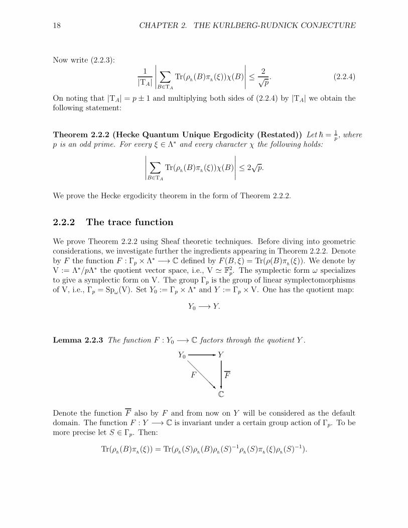
Lemma 2.2.3 The function F : Y0 −→ C factors through the quotient Y .
Y0 Y✲
F
❅❅❅❅❅❘
C❄
F
Denote the function F also by F and from now on Y will be considered as the defaultdomain. The function F : Y −→ C is invariant under a certain group action of Γp. To bemore precise let S ∈ Γp. Then:
Tr(ρ~(B)π
~(ξ)) = Tr(ρ
~(S)ρ
~(B)ρ
~(S)−1ρ
~(S)π
~(ξ)ρ
~(S)−1).
2.2. PROOF OF THE KURLBERG-RUDNICK CONJECTURE 19
Applying the Egorov identity (1.2.1) and using the fact that ρ~is a representation we get:
Tr(ρ~(S)ρ
~(B)ρ
~(S)−1ρ
~(S)π
~(ξ)ρ
~(S)−1) = Tr(π
~(Sξ)ρ
~(SBS−1)).
Altogether we have:F (B, ξ) = F (SBS−1, Sξ). (2.2.5)
Putting (2.2.5) in a more diagrammatic form: there is an action of Γp on Y given by thefollowing formula:
Γp × Y α−−−→ Y,
(S, (B, ξ)) −−−→ (SBS−1, Sξ).(2.2.6)
Consider the following diagram:
Ypr←−−− Γp × Y α−−−→ Y
where pr is the projection on the Y variable. Formula (2.2.5) can be stated equivalentlyas:
α∗(F ) = pr∗(F )
where α∗(F ) and pr∗(F ) are the pullbacks of the function F on Y via the maps α and prrespectively.
2.2.3 Geometrization (Sheafification)
Next, we will phrase a geometric statement that will imply Theorem 2.2.2. Moving intothe geometric setting, we replace the set Y by an algebraic variety and the functions Fand χ by sheaf theoretic objects, also of a geometric flavor.
Step 1. The set Y is not an arbitrary finite set but it is the set of rational pointsof an algebraic variety Y defined over Fp. To be more precise, Y ≃ Spω ×V. The varietyY is equipped with an endomorphism:
Fr : Y −→ Y
called Frobenius. The set Y is identified with the set of fixed points of Frobenius:
Y = YFr = {y ∈ Y : Fr(y) = y}.
Note that the finite group Γp is the set of rational points of the algebraic group Spω. Thevector space V is the set of rational points of the variety V, where V is isomorphic to theaffine plane A2. We denote by α the action of Spω on the variety Y (cf. (2.2.6)).
Having all finite sets replaced by corresponding algebraic varieties, we replace functions
20 CHAPTER 2. THE KURLBERG-RUDNICK CONJECTURE
by sheaf theoretic objects as shown.
Step 2. The following theorem proposes an appropriate sheaf theoretic object stand-ing in place of the function F : Y −→ C. Denote by Dbc,w(Y) the bounded derivedcategory of constructible ℓ-adic Weil sheaves on Y (cf. [M, BBD], in addition see [BL] forequivariant sheaves theory).
Theorem 2.2.4 (Geometrization Theorem) There exists an object F ∈ Dbc,w(Y) sat-isfying the following properties:
1. (Function) It is associated, via the sheaf-to-function correspondence, to the functionF : Y −→ C:
fF = F.
2. (Weight) It is of weight:w(F) ≤ 0.
3. (Equivariance) For every element S ∈ Spω there exists an isomorphism
α∗SF ≃ F .
4. (Formula) On introducing coordinates V ≃ A2 we identify Spω ≃ SL2. Then thereexists an isomorphism:
F|T×V≃ Lψ( 1
2λµ a+1
a−1) ⊗Lσ(a).
3
Here T := {(
a 00 a−1
)
} stands for the standard torus and (λ, µ) are the coordinates onV.
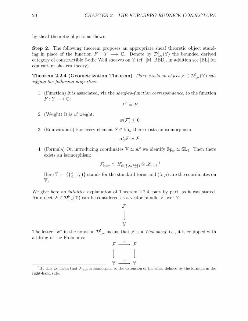
We give here an intuitive explanation of Theorem 2.2.4, part by part, as it was stated.An object F ∈ Dbc,w(Y) can be considered as a vector bundle F over Y:
F
y
Y
The letter “w” in the notation Dbc,w means that F is a Weil sheaf, i.e., it is equipped witha lifting of the Frobenius:
F Fr−−−→ F
y
y
YFr−−−→ Y
3By this we mean that F|T×Vis isomorphic to the extension of the sheaf defined by the formula in the
right-hand side.
2.2. PROOF OF THE KURLBERG-RUDNICK CONJECTURE 21
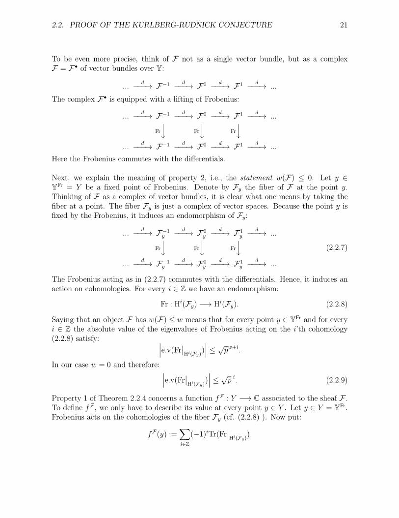
To be even more precise, think of F not as a single vector bundle, but as a complexF = F• of vector bundles over Y:
...d−−−→ F−1 d−−−→ F0 d−−−→ F1 d−−−→ ...
The complex F• is equipped with a lifting of Frobenius:
...d−−−→ F−1 d−−−→ F0 d−−−→ F1 d−−−→ ...
Fr
yFr
yFr
y
...d−−−→ F−1 d−−−→ F0 d−−−→ F1 d−−−→ ...
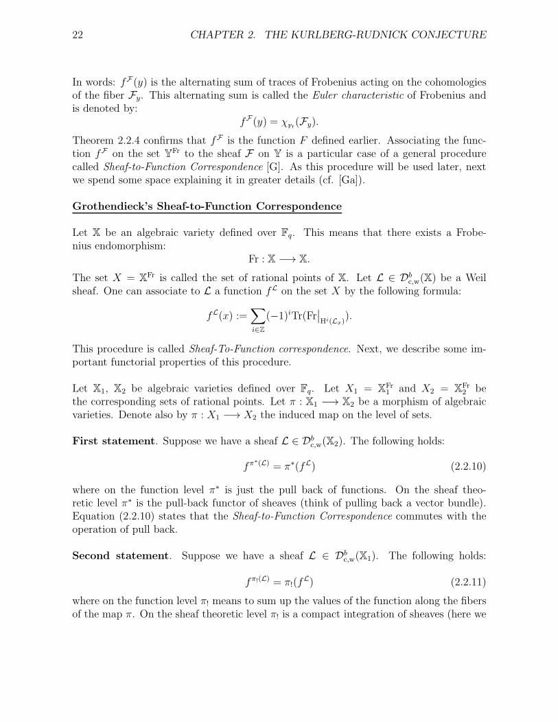
Here the Frobenius commutes with the differentials.
Next, we explain the meaning of property 2, i.e., the statement w(F) ≤ 0. Let y ∈YFr = Y be a fixed point of Frobenius. Denote by Fy the fiber of F at the point y.Thinking of F as a complex of vector bundles, it is clear what one means by taking thefiber at a point. The fiber Fy is just a complex of vector spaces. Because the point y isfixed by the Frobenius, it induces an endomorphism of Fy:
...d−−−→ F−1
yd−−−→ F0
yd−−−→ F1
yd−−−→ ...
Fr
yFr
yFr
y
...d−−−→ F−1
yd−−−→ F0
yd−−−→ F1
yd−−−→ ...
(2.2.7)
The Frobenius acting as in (2.2.7) commutes with the differentials. Hence, it induces anaction on cohomologies. For every i ∈ Z we have an endomorphism:
Fr : Hi(Fy) −→ Hi(Fy). (2.2.8)
Saying that an object F has w(F) ≤ w means that for every point y ∈ YFr and for everyi ∈ Z the absolute value of the eigenvalues of Frobenius acting on the i’th cohomology(2.2.8) satisfy:
∣
∣
∣e.v(Fr
∣
∣
Hi(Fy))∣
∣
∣≤ √pw+i.
In our case w = 0 and therefore:∣
∣
∣e.v(Fr
∣
∣
Hi(Fy))∣
∣
∣≤ √p i. (2.2.9)
Property 1 of Theorem 2.2.4 concerns a function fF : Y −→ C associated to the sheaf F .To define fF , we only have to describe its value at every point y ∈ Y . Let y ∈ Y = YFr.Frobenius acts on the cohomologies of the fiber Fy (cf. (2.2.8) ). Now put:
fF(y) :=∑
i∈Z(−1)iTr(Fr
∣
∣
Hi(Fy)).
22 CHAPTER 2. THE KURLBERG-RUDNICK CONJECTURE
In words: fF(y) is the alternating sum of traces of Frobenius acting on the cohomologiesof the fiber Fy. This alternating sum is called the Euler characteristic of Frobenius andis denoted by:
fF(y) = χFr(Fy).
Theorem 2.2.4 confirms that fF is the function F defined earlier. Associating the func-tion fF on the set YFr to the sheaf F on Y is a particular case of a general procedurecalled Sheaf-to-Function Correspondence [G]. As this procedure will be used later, nextwe spend some space explaining it in greater details (cf. [Ga]).
Grothendieck’s Sheaf-to-Function Correspondence
Let X be an algebraic variety defined over Fq. This means that there exists a Frobe-nius endomorphism:
Fr : X −→ X.
The set X = XFr is called the set of rational points of X. Let L ∈ Dbc,w(X) be a Weilsheaf. One can associate to L a function fL on the set X by the following formula:
fL(x) :=∑
i∈Z(−1)iTr(Fr
∣
∣
Hi(Lx)).
This procedure is called Sheaf-To-Function correspondence. Next, we describe some im-portant functorial properties of this procedure.
Let X1, X2 be algebraic varieties defined over Fq. Let X1 = XFr1 and X2 = XFr
2 bethe corresponding sets of rational points. Let π : X1 −→ X2 be a morphism of algebraicvarieties. Denote also by π : X1 −→ X2 the induced map on the level of sets.
First statement. Suppose we have a sheaf L ∈ Dbc,w(X2). The following holds:
fπ∗(L) = π∗(fL) (2.2.10)
where on the function level π∗ is just the pull back of functions. On the sheaf theo-retic level π∗ is the pull-back functor of sheaves (think of pulling back a vector bundle).Equation (2.2.10) states that the Sheaf-to-Function Correspondence commutes with theoperation of pull back.
Second statement. Suppose we have a sheaf L ∈ Dbc,w(X1). The following holds:
fπ!(L) = π!(fL) (2.2.11)
where on the function level π! means to sum up the values of the function along the fibersof the map π. On the sheaf theoretic level π! is a compact integration of sheaves (here we
2.2. PROOF OF THE KURLBERG-RUDNICK CONJECTURE 23
have no analogue under the vector bundle interpretation). Equation (2.2.11) states thatthe Sheaf-to-Function Correspondence commutes with integration.
Third statement. Suppose we have two sheaves L1,L2 ∈ Dbc,w(X1). The followingholds:
fL1⊗L2 = fL1 · fL2. (2.2.12)
In words: Sheaf-to-Function Correspondence takes tensor product of sheaves to multipli-cation of the corresponding functions.
2.2.4 Geometric statement
Fix an element ξ ∈ Λ∗ with ξ 6= 0. We denote by iξthe inclusion map i
ξ: TA × ξ −→ Y .
Going back to Theorem 2.2.2 and putting its content in a functorial notation, we writethe following inequality:
∣
∣
∣pr!(i
∗ξ(F ) · χ)
∣
∣
∣≤ 2√p.
In words, taking the function F : Y −→ C and:
• Restrict F to TA × ξ and get i∗ξ(F ).
• Multiply i∗ξF by the character χ to get i∗
ξ(F ) · χ.
• Integrate i∗ξ(F ) ·χ to the point, this means to sum up all its values, and get a scalar
aχ := pr!(i∗ξ(F ) · χ). Here pr stands for the projection pr : TA × ξ −→ pt.
Then Theorem 2.2.2 asserts that the scalar aχ is of an absolute value less than 2√p.
Repeat the same steps in the geometric setting. We denote again by iξthe closed imbed-
ding iξ: TA × ξ −→ Y. Take the sheaf F on Y and apply the following sequence of
operations:
• Pull-back F to the closed subvariety TA × ξ and get the sheaf i∗ξ(F).
• Take the tensor product of i∗ξ(F) with the Kummer sheaf Lχ and get i∗
ξ(F)⊗Lχ.
• Integrate i∗ξ(F)⊗Lχ to the point and get the sheaf pr!(i
∗ξ(F)⊗Lχ) on the point.
The Kummer sheaf Lχ is the character sheaf (cf. [Ga]) associated via Sheaf-to-Function
Correspondence to the character χ.
24 CHAPTER 2. THE KURLBERG-RUDNICK CONJECTURE
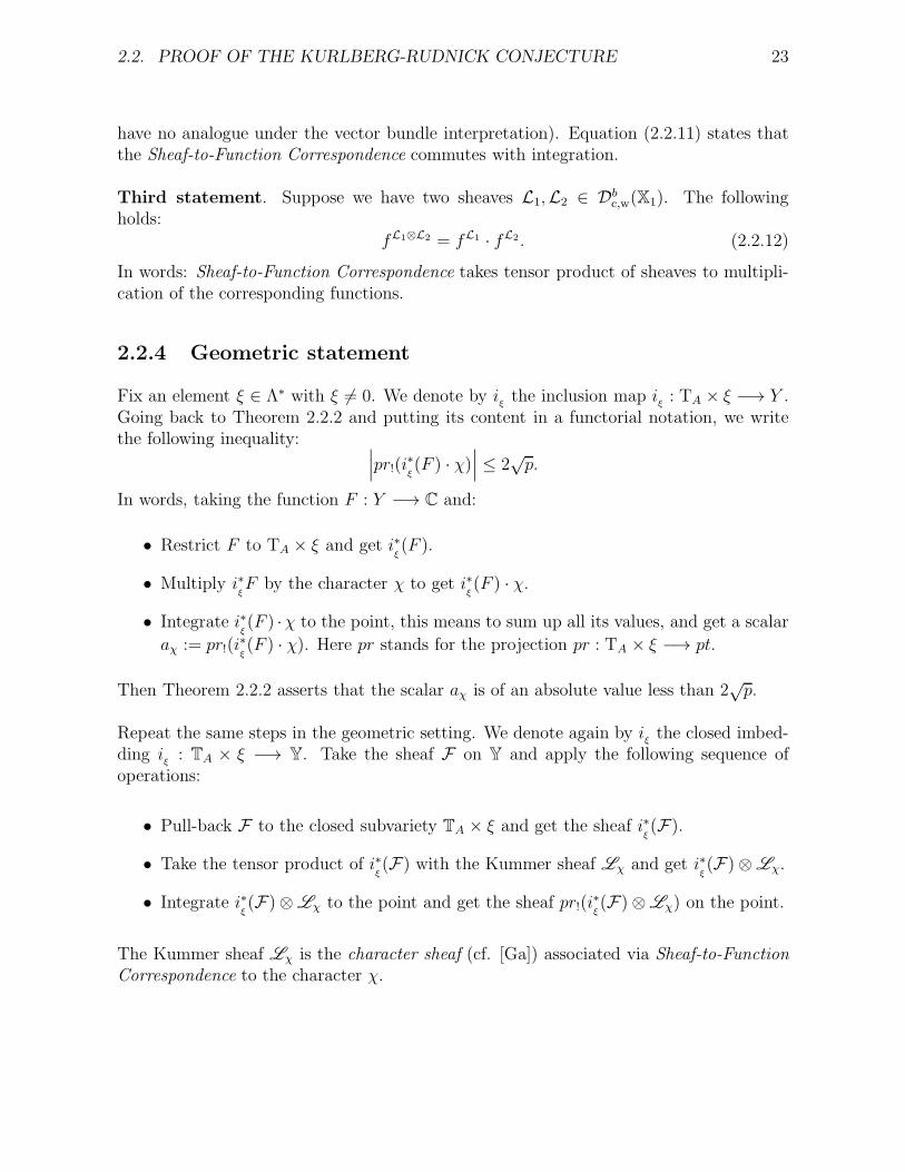
The operation of Sheaf-to-Function Correspondence commutes both with pullback (2.2.10),with integration (2.2.11) and takes the tensor product of sheaves to the multiplication offunctions (2.2.12). This means that it intertwines the operations carried out on the level ofsheaves with those carried out on the level of functions. The following diagram describespictorially what has been said so far:
F χFr−−−→ F
iξ
x
iξ
x
i∗ξ(F)⊗Lχ
χFr−−−→ i∗
ξ(F ) · χ
pr
y
pr
y
pr!(i∗ξ(F)⊗Lχ)
χFr−−−→ pr!(i
∗ξ(F ) · χ)
Recall w(F) ≤ 0. Now, the effect of functors i∗ξ, pr! and tensor product ⊗ on the property
of weight should be examined.
The functor i∗ξdoes not increase weight. Observing the definition of weight this claim
is immediate. Therefore we get:
w(i∗ξ(F)) ≤ 0.
Assume we have two sheaves L1 and L2 with weights w(L1) ≤ w1and w(L2) ≤ w
2. The
weight of the tensor product satisfies w(L1 ⊗ L2) ≤ w1+ w
2. This is again immediate
from the definition of weight.
Knowing that the Kummer sheaf has weight w(Lχ) ≤ 0 we deduce:
w(i∗ξ(F)⊗Lχ) ≤ 0.
Finally, one has to understand the affect of the functor pr!. The following theorem,proposed by Deligne [D2], is a very deep and important result in the theory of weights.Briefly speaking, the theorem states that compact integration of sheaves does not increaseweight. Here is the precise statement:
Theorem 2.2.5 (Deligne, Weil II [D2]) Let π : X1 −→ X2 be a morphism of algebraic
varieties. Let L ∈ Dbc,w(X1) be a sheaf of weight w(L) ≤ w then w(π!(L)) ≤ w.
Using Theorem 2.2.5 we get:
w(pr!(i∗ξ(F)⊗Lχ)) ≤ 0.
2.2. PROOF OF THE KURLBERG-RUDNICK CONJECTURE 25
Consider the sheaf G := pr!(i∗ξ(F) ⊗ Lχ). It is an object in Dbc,w(pt). This means it is
merely a complex of vector spaces, G = G•, together with an action of Frobenius:
...d−−−→ G−1 d−−−→ G0 d−−−→ G1 d−−−→ ...
Fr
yFr
yFr
y
...d−−−→ G−1 d−−−→ G0 d−−−→ G1 d−−−→ ...
The complex G• is associated by Sheaf-To-Function correspondence to the scalar aχ:
aχ =∑
i∈Z(−1)iTr(Fr
∣
∣
Hi(G)). (2.2.13)
Finally, we can give the geometric statement about G, which will imply Theorem 2.2.2.
Lemma 2.2.6 (Vanishing Lemma) Let G = pr!(i∗ξ(F)⊗Lχ). All cohomologies Hi(G)
vanish except for i = 1. Moreover, H1(G) is a two dimensional vector space.
Theorem 2.2.2 now follows easily. By Lemma 2.2.6 only the first cohomology H1(G)does not vanish and it is two dimensional. Having w(G) ≤ 0 implies (cf. 2.2.9) thatthe eigenvalues of Frobenius acting on H1(G) are of absolute value ≤ √p. Hence, usingformula (2.2.13) we get:
|aχ| ≤ 2√p.
The remainder of the chapter is devoted to the proof of Lemma 2.2.6.
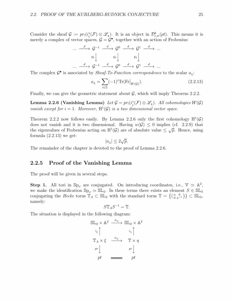
2.2.5 Proof of the Vanishing Lemma
The proof will be given in several steps.
Step 1. All tori in Spω are conjugated. On introducing coordinates, i.e., V ≃ A2,we make the identification Spω ≃ SL2. In these terms there exists an element S ∈ SL2
conjugating the Hecke torus TA ⊂ SL2 with the standard torus T ={
( a 00 a−1
)
} ⊂ SL2,namely:
STAS−1 = T.
The situation is displayed in the following diagram:
SL2 × A2αS−−−→ SL2 × A2
iξ
x
iη
x
TA × ξαS−−−→ T× η
pr
y
pr
y
pt pt
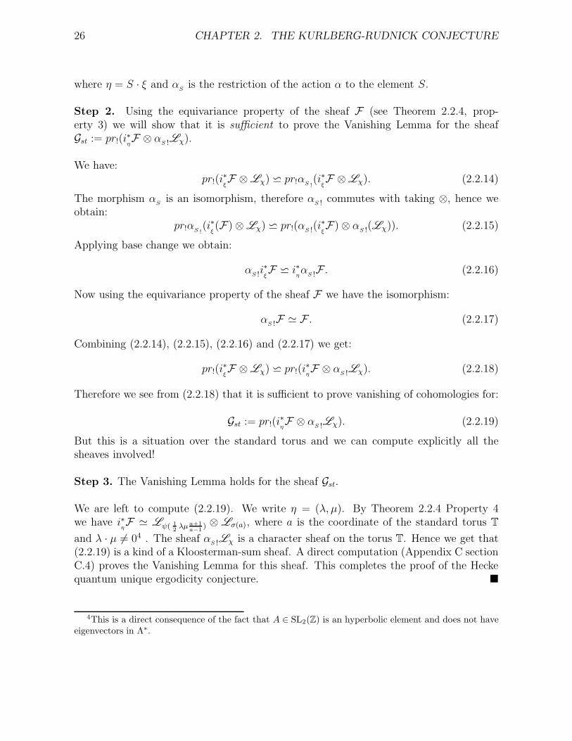
26 CHAPTER 2. THE KURLBERG-RUDNICK CONJECTURE
where η = S · ξ and αSis the restriction of the action α to the element S.
Step 2. Using the equivariance property of the sheaf F (see Theorem 2.2.4, prop-erty 3) we will show that it is sufficient to prove the Vanishing Lemma for the sheafGst := pr!(i
∗ηF ⊗ α
S !Lχ).
We have:pr!(i
∗ξF ⊗Lχ) ⋍ pr!αS !
(i∗ξF ⊗Lχ). (2.2.14)
The morphism αSis an isomorphism, therefore α
S ! commutes with taking ⊗, hence weobtain:
pr!αS !(i∗
ξ(F)⊗Lχ) ⋍ pr!(αS !(i
∗ξF)⊗ α
S !(Lχ)). (2.2.15)
Applying base change we obtain:
αS !i
∗ξF ⋍ i∗
ηα
S !F . (2.2.16)
Now using the equivariance property of the sheaf F we have the isomorphism:
αS !F ≃ F . (2.2.17)
Combining (2.2.14), (2.2.15), (2.2.16) and (2.2.17) we get:
pr!(i∗ξF ⊗Lχ) ⋍ pr!(i
∗ηF ⊗ α
S !Lχ). (2.2.18)
Therefore we see from (2.2.18) that it is sufficient to prove vanishing of cohomologies for:
Gst := pr!(i∗ηF ⊗ α
S !Lχ). (2.2.19)
But this is a situation over the standard torus and we can compute explicitly all thesheaves involved!
Step 3. The Vanishing Lemma holds for the sheaf Gst.
We are left to compute (2.2.19). We write η = (λ, µ). By Theorem 2.2.4 Property 4we have i∗
ηF ≃ Lψ( 1
2λµ a+1
a−1) ⊗ Lσ(a), where a is the coordinate of the standard torus T
and λ · µ 6= 04 . The sheaf αS !Lχ is a character sheaf on the torus T. Hence we get that
(2.2.19) is a kind of a Kloosterman-sum sheaf. A direct computation (Appendix C sectionC.4) proves the Vanishing Lemma for this sheaf. This completes the proof of the Heckequantum unique ergodicity conjecture. �
4This is a direct consequence of the fact that A ∈ SL2(Z) is an hyperbolic element and does not haveeigenvectors in Λ∗.

Chapter 3
Metaplectique
In the first part of this chapter we give new construction of theWeil (metaplectic) represen-tation (ρ, Sp(V),HV), attached to a two dimensional symplectic vector space (V, ω) overFq, which appears in the body of the thesis. The difference is that here the constructionis slightly more general. But even more importantly, it is obtained in completely naturalgeometric terms. The focal step in our approach is the introduction of a canonical Hilbert
space on which the Weil representation is naturally manifested. The motivation to lookfor this space was initiated by a question of David Kazhdan [Ka]. The key idea behindthis construction was suggested to us by Joseph Bernstein [B]. The upshot is to replacethe notion of a Lagrangian subspace by a more refined notion of an oriented Lagrangian
subspace 1.
In the second part of this chapter we apply a geometrization procedure to the construc-tion given in the first part, meaning that all sets are replaced by algebraic varieties andall functions are replaced by ℓ-adic sheaves. This part is based on a letter of Deligne toKazhdan from 1982 [D1]. We extract from that work only the part that is most relevantto this thesis. Although all basic ideas appear already in the letter, we tried to give herea slightly more general and detailed account of the construction. As far as we know,the contents of this mathematical work has never been published. This might be a goodenough reason for writing this part.
The following is a description of the chapter. In section 3.1 we introduce the notionof oriented Lagrangian subspace and the construction of the canonical Hilbert space. Insection 3.2 we obtain a natural realization of the Weil representation. In section 3.3 wegive the standard Schrodinger realization (cf. [W2]). We also include several formulasfor the kernels of basic operators. These formulas will be used in section 3.4 where the
1We thank A. Polishchuk for pointing out to us that this is an Fq-analogue of well known considerationswith usual oriented Lagrangians giving explicitly the metaplectic covering of Sp(2n,R) (cf. [LV]).
27
28 CHAPTER 3. METAPLECTIQUE
geometrization procedure is described. In section 3.5 we give proofs of all lemmas andpropositions which appear in previous sections.
For the remainder of this chapter we fix the following notations. Let Fq denote thefinite field of characteristic p 6= 2 and q elements. Fix ψ : Fq −→ C∗ a non-trivial additivecharacter. Denote by σ : F∗
q −→ C∗ the Legendre multiplicative quadratic character.
3.1 Canonical Hilbert space
3.1.1 Oriented Lagrangian subspace
Let (V, ω) be a 2-dimensional symplectic vector space over Fq.
Definition 3.1.1 An oriented Lagrangian subspace is a pair (L, L), where L is a La-
grangian subspace of V and L
: L r {0} −→ {±1} is a function which satisfies the
following equivariant property:
L(t · l) = σ(t)
L(l)
where t ∈ F∗q and σ the Legendre character of F∗
q.
We denote by Lag◦ the space of oriented Lagrangians subspaces. There is a forgetful mapLag◦ −→ Lag, where Lag is the space of Lagrangian subspaces, Lag ≃ P1(Fq). In thesequel we use the notation L◦ to specify that L is equipped with an orientation.
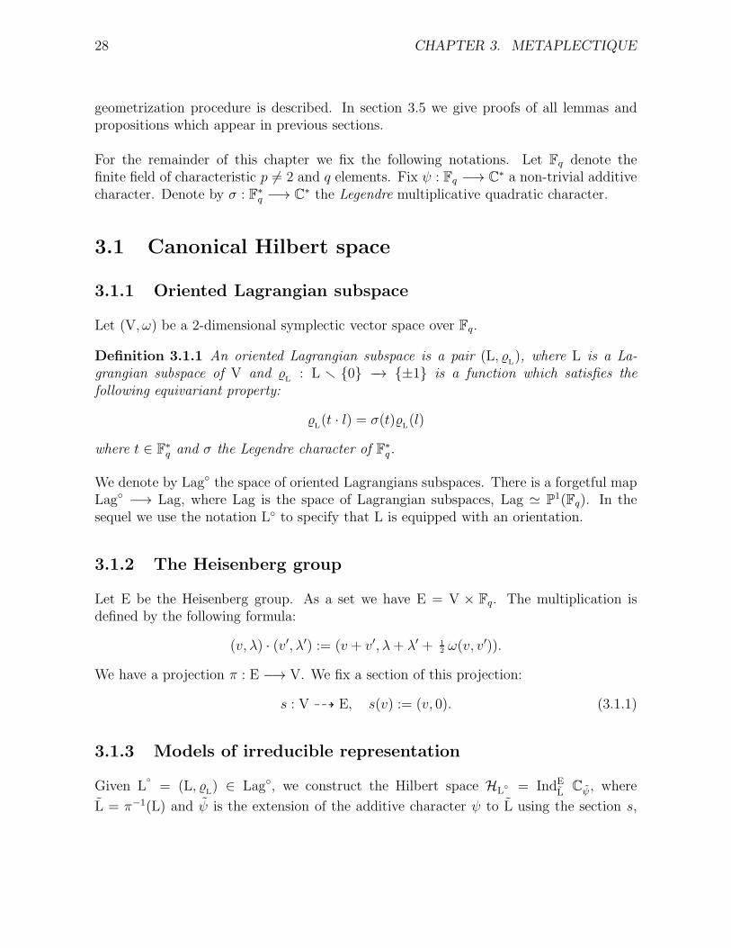
3.1.2 The Heisenberg group
Let E be the Heisenberg group. As a set we have E = V × Fq. The multiplication isdefined by the following formula:
(v, λ) · (v′, λ′) := (v + v′, λ+ λ′ + 12 ω(v, v
′)).
We have a projection π : E −→ V. We fix a section of this projection:
s : V 99K E, s(v) := (v, 0). (3.1.1)
3.1.3 Models of irreducible representation
Given L◦= (L,
L) ∈ Lag◦, we construct the Hilbert space HL◦ = IndE
LCψ, where
L = π−1(L) and ψ is the extension of the additive character ψ to L using the section s,
3.1. CANONICAL HILBERT SPACE 29
i.e., ψ : L = L× Fq −→ C∗ is given by the formula:
ψ(l, λ) := ψ(λ).
More concretely: HL◦ = {f : E −→ C | f(λle) = ψ(λ)f(e)}. The group E acts on HL◦ bymultiplication from the right. It is well known (and easy to prove) that the representationsHL◦ of E are irreducible and for different L
◦’s they are all isomorphic. These are different
models of the same irreducible representation. This is stated in the following theorem:
Theorem 3.1.2 (Stone-von Neumann) For an oriented Lagrangian subspace L◦, the
representation HL◦ of E is irreducible. Moreover, for any two oriented Lagrangians
L◦
1,L◦
2 ∈ Lag◦ one has HL◦1≃ HL
◦2as representations of E. �
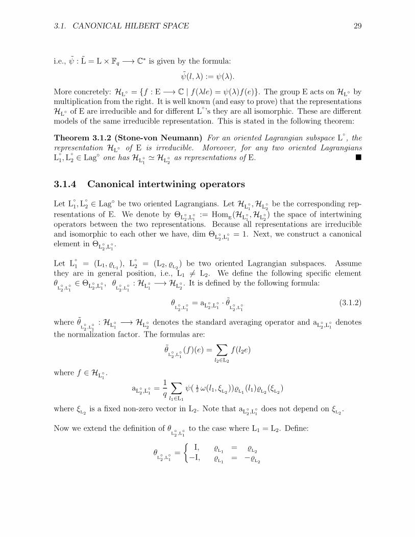
3.1.4 Canonical intertwining operators
Let L◦
1,L◦
2 ∈ Lag◦ be two oriented Lagrangians. Let HL◦1,HL
◦2be the corresponding rep-
resentations of E. We denote by ΘL◦2 ,L
◦1:= Hom
E(HL
◦1,HL
◦2) the space of intertwining
operators between the two representations. Because all representations are irreducibleand isomorphic to each other we have, dim ΘL
◦2 ,L
◦1= 1. Next, we construct a canonical
element in ΘL◦2 ,L
◦1.
Let L◦
1 = (L1, L1), L
◦
2 = (L2, L2) be two oriented Lagrangian subspaces. Assume
they are in general position, i.e., L1 6= L2. We define the following specific elementθL◦2,L
◦1
∈ ΘL◦2 ,L
◦1, θ
L◦2,L
◦1
: HL◦1−→ HL
◦2. It is defined by the following formula:
θL◦2,L
◦1
= aL◦2 ,L
◦1· θ
L◦2,L
◦1
(3.1.2)
where θL◦2,L
◦1
: HL◦1−→ HL
◦2denotes the standard averaging operator and aL◦
2 ,L◦1denotes
the normalization factor. The formulas are:
θL◦2,L
◦1
(f)(e) =∑
l2∈L2
f(l2e)
where f ∈ HL◦1.
aL◦2 ,L
◦1=
1
q
∑
l1∈L1
ψ( 12 ω(l1, ξL2
))L1(l1)L2
(ξL2)
where ξL2
is a fixed non-zero vector in L2. Note that aL◦2 ,L
◦1does not depend on ξ
L2.
Now we extend the definition of θL◦2,L
◦1
to the case where L1 = L2. Define:
θL◦2,L
◦1
=
{
I, L1
= L2
−I, L1
= −L2
30 CHAPTER 3. METAPLECTIQUE
The main claim is that the collection {θL◦2,L
◦1
}L◦1,L
◦2∈Lag◦
is associative. This is formulated
in the following theorem:
Theorem 3.1.3 (Associativity) Let L◦
1,L◦
2,L◦
3 ∈ Lag◦ be a triple of oriented Lagrangian
subspaces. The following associativity condition holds:
θL◦3,L
◦2
◦ θL◦2,L
◦1
= θL◦3,L
◦1
.
3.1.5 Canonical Hilbert space
Define the canonical Hilbert spaceHV ⊂⊕
L◦∈Lag◦HL◦ as the subspace of compatible systems
of vectors, namely:
HV := {(fL◦ )
L◦∈Lag◦
; θL◦2,L
◦1
(fL◦1
) = fL◦2
}.
3.2 The Weil representation
In this section we construct the Weil representation using the Hilbert space HV. Wedenote by Spω := Sp(V, ω) the group of linear symplectomorphisms of V. Before givingany formulas, note that the space HV was constructed out of the symplectic space (V, ω)in a complete canonical way. This immediately implies that all the symmetries of (V, ω)automatically act on HV. In particular, we obtain a linear representation of the groupSpω in the space HV. This is the famous Weil representation of Spω and we denote it byρ : Spω −→ GL(HV). It is given by the following formula:
ρ(g)[(fL◦ )] := (f g
L◦). (3.2.1)
Let us elaborate on this formula. The group Spω acts on the space Lag◦. Any elementg ∈ Spω induces an automorphism g : Lag◦ −→ Lag◦ defined by:
(L, L) 7−→ (gL, g
L)
where gL(l) =
L(g−1l). Moreover, g induces an isomorphism of vector spaces g : HL
◦ −→HgL◦ defined by the following formula:
fL◦ 7−→ f g
L◦, f g
L◦(e) := f
L◦ (g
−1e) (3.2.2)
where the action of g ∈ Spω on e = (v, λ) ∈ E is given by g(v, λ) = (gv, λ). It iseasy to verify that the action (3.2.2) of Spω commutes with the canonical intertwining
3.3. REALIZATION AND FORMULAS 31
operators, i.e., for any two L◦
1,L◦
2 ∈ Lag◦ and any element g ∈ Spω the following diagramis commutative:
HL◦1
θL◦2,L
◦1−−−−→ HL
◦2
g
y
g
y
HgL◦1
θgL
◦2,gL
◦1−−−−−→ HgL
◦2
From this we deduce that formula (3.2.1) indeed gives the action of Spω on HV.
3.3 Realization and formulas
In this section we give the standard Schrodinger realization of the Weil representation.Several formulas for the kernels of basic operators are also included.
3.3.1 Schrodinger realization
Fix V = V1 ⊕ V2 to be a Lagrangian decomposition of V. Fix V2
to be an orientation
on V2. Denote by V◦
2 = (V2, V2) the oriented space. Using the system of canonical
intertwining operators we identify HV with a specific representative HV◦2. Using the
section s : V 99K E (cf. 3.1.1) we further make the identification s : HV◦2≃ S(V1), where
S(V1) is the space of complex valued functions on V1. We denote H := S(V1). In thisrealization the Weil representation, ρ : Spω −→ GL(H), is given by the following formula:
ρ(g)(f) = θV◦2,gV
◦2
(f g)
where f ∈ H ≃ HV◦2and g ∈ Spω.
3.3.2 Formulas for the Weil representation
First we introduce a basis e ∈ V1 and the dual basis e∗ ∈ V2 normalized so thatω(e, e∗) = 1. In terms of this basis we have the following identifications: V ≃ F2
q,V1,V2 ≃ Fq, Spω ≃ SL2(Fp) and E ≃ F2
q × Fq (as sets). We also have H ≃ S(Fq).
For every element g ∈ Spω the operator ρ(g) : H −→ H is represented by a kernel Kg :F2q −→ C. The multiplication of operators becomes convolution of kernels. The collection{Kg}g∈Spω gives a single function of “kernels” which we denote by Kρ : Spω × F2
q −→ C.For every element g ∈ Spω the kernel Kρ(g) is of the form:
Kρ(g, x, y) = ag · ψ(Rg(x, y))
32 CHAPTER 3. METAPLECTIQUE
where ag is a certain normalizing coefficient and Rg : F2q −→ Fq is a quadratic function
supported on some linear subspace of F2q. Next, we give an explicit description of the
kernels Kρ(g).
Consider the (opposite) Bruhat decomposition Spω = BwB ∪ B where:
B :=
(
∗∗ ∗
)
and w := ( 0 1−1 0 ) is the standard Weyl element.
If g ∈ BwB then:
g =
(
a bc d
)
where b 6= 0. In this case we have:
ag =1
q
∑
t∈Fq
ψ(b
2t)σ(t),
Rg(x, y) =−b−1d
2x2 +
b−1 − c+ ab−1d
2xy − ab−1
2y2.
Altogether we have:
Kρ(g, x, y) = ag · ψ(−b−1d
2x2 +
b−1 − c+ ab−1d
2xy − ab−1
2y2).
If g ∈ B then:
g =
(
a 0r a−1
)
.
In this case we have:
ag = σ(a),
Rg(x, y) =−ra−1
2x2 · δy=a−1x.
Altogether we have:
Kρ(g, x, y) = ag · ψ(−ra−1
2x2)δy=a−1x. (3.3.1)
3.3.3 Formulas for the Heisenberg representation
On H we also have a representation of the Heisenberg group E. We denote it byπ : E −→ GL(H). For every element e ∈ E we have a kernel Ke : F2
q −→ C. We
3.4. DELIGNE’S LETTER 33
denote by Kπ : E × F2q −→ C the function of kernels. For an element e ∈ E the kernel
Kπ(e) has the form ψ(Re(x, y)) where Re is an affine function which is supported on acertain one dimensional subspace of F2
q. Here are the exact formulas:
For an element e = (q, p, λ) we have:
Re(x, y) = (pq
2+ px+ λ)δy=x+q,
Kπ(e, x, y) = ψ(pq
2+ px+ λ)δy=x+q. (3.3.2)
3.3.4 Formulas for the representation of the semi-direct product
The representations ρ : Spω −→ GL(H) and π : E −→ GL(H) combine together to give arepresentation of the semi-direct product D = Spω ⋉ E. We denote the total representa-tion by ρ⋉ π : D −→ GL(H), ρ⋉ π(g, e) = ρ(g) · π(e). The representation ρ⋉ π is givenby a kernel Kρ⋉π : D× F2
q −→ C. We denote this kernel simply by K.
We give an explicit formula for the kernel K only in the case (g, e) ∈ BwB× E, i.e.,
g =
(
a bc d
)
where b 6= 0 and e = (q, p, λ). In this case:
R(g, e, x, y) = Rg(x, y − q) +Re(y − q, y), (3.3.3)
K(g, e, x, y) = ag · ψ(Rg(x, y − q) +Re(y − q, y)). (3.3.4)
3.4 Deligne’s letter
In this section we geometrize (Theorem 3.4.2) the total representation ρ ⋉ π : D −→ H.First, we realize all finite sets as rational points of certain algebraic varieties. Vectorspaces: V = V(Fq), V1 = V1(Fq). Groups: E = E(Fq), where E = V×Ga, Spω = Spω(Fq)and finally D = D(Fq), where D = Spω × E. The second step is to replace the kernel
K := Kρ⋉π : D× F2q −→ C (see (3.3.4)) by sheaf theoretic object. Recall that the kernel
K is a representation kernel, namely it is a kernel of a representation and hence satisfiesthe convolution property:
m∗K = K ∗K (3.4.1)
wherem : D×D −→ D denotes the multiplication map and ∗means convolution of kernels,i.e., matrix multiplication. We replace the kernel K by Deligne’s Weil representation
34 CHAPTER 3. METAPLECTIQUE
sheaf [D1]. This is an object K ∈ Dbc,w(D × A2) that satisfies2 the analogue (to (3.4.1))convolution property:
m∗K ⋍ K ∗ K
and its function is:
fK = K.
Here m : D× D −→ D denotes the multiplication morphism and ∗ means convolution ofsheaves.
3.4.1 Uniqueness and existence of the Weil representation sheaf
The strategy
The method of constructing the Weil representation sheaf K is close in spirit to theconstruction of an analytic function via analytic continuation. In the realm of perversesheaves one uses the operation of perverse extension (cf. [BBD]). The main idea is toconstruct, using formulas, an explicit irreducible perverse sheaf KO on a ”good” opensubvariety O ⊂ D × A2 and then to obtain the sheaf K by perverse extension of KO tothe whole variety D× A2.
Explicit construction on open subvariety
On introducing coordinates we get: V ≃ A2, V1 ⋍ A1 and Spω ≃ SL2. We denote by O
the open subvariety:
O := Ow × E× A2
where Ow denotes the (opposite) big Bruhat cell BwB ⊂ SL2.
Let us fix some standard notations from the theory of ℓ-adic sheaves (see [BBD] forthe notions of ℓ-adic sheaves). We denote by Lψ the Artin-Schreier sheaf on the groupGa that corresponds to the character ψ. We denote by Lσ the Kummer sheaf on themultiplicative group Gm that corresponds to the Legendre character σ. In the sequel wewill frequently make use of the character property (cf. [Ga]) of the sheaves Lψ and Lσ,namely:
s∗Lψ ≃ Lψ ⊠Lψ, (3.4.2)
m∗Lσ ≃ Lσ ⊠Lσ (3.4.3)
2However, in this work we will prove a weaker property (see Theorem 3.4.2) which is sufficient for ourpurposes.
3.4. DELIGNE’S LETTER 35
where s : Ga×Ga −→ Ga and m : Gm×Gm −→ Gm denote the addition and multiplicationmorphisms correspondingly, and ⊠ means exterior tensor product of sheaves.
At last, given a sheaf L we use the notation L[i] for the translation functors and thenotation L(i) for the i’th Tate twist.
The construction of the explicit sheaf KO
We sheafify the kernel Kρ⋉π of the total representation, when restricted to the set O :=Ow × E × F2
q, using the formula (3.3.4). We obtain a sheaf on the open subvarietyOw × E× A2, which we denote by KO. We define:
KO := AO ⊗ KO
where KO is the sheaf of the non-normalized kernels and AO is the sheaf of the normaliza-tion coefficients. The sheaves KO and AO are constructed as follows: define the morphismR : Ow × E × A2 −→ A1 by formula (3.3.3) and let pr : Ow × E × A2 −→ Ow be theprojection morphism. Now take:
KO := R∗Lψ,
AO := pr∗AOw
where:
AOw := pr1!(ν∗Lψ ⊗ pr∗2Lσ)[2](1).
Here ν : Ow × A1 −→ A1 is the morphism defined by ν(g, t) = 12 bt, where g = ( a bc d ), and
pr1 : Ow × A1 −→ Ow, pr2 : Ow × A1 −→ A1 denote the natural projections on the firstand second coordinates correspondingly. From the construction we deduce:
Corollary 3.4.1 The sheaf KO is perverse irreducible of pure weight zero and its function
agrees with K on O, i.e., fKO = K|O .
Main theorem
We are now ready to state and prove the main theorem of this section:
Theorem 3.4.2 (Weil representation sheaf [D1]) There exists a unique (up to isomorphism)object K ∈ Dbc,w(D× A2) which satisfies the following properties:
1. (Restriction) There exists an isomorphism K|O ≃ KO.
36 CHAPTER 3. METAPLECTIQUE
2. (Convolution property) For every element g ∈ D there exists isomorphisms:
K|g ∗ K ≃ L∗g(K)
and:K ∗ K|g ≃ R∗
g(K).Here K|g denotes the restriction of K to the subvariety g×A2, ∗ means convolutionof sheaves and Rg, Lg : D −→ D are the morphisms of right and left multiplicationby g respectively.
Corollary 3.4.3 The Weil representation sheaf K has the following two properties:
a. (Function) fK = K.
b. (Weight) ω(K) = 0.
Proof (of Theorem 3.4.2). Uniqueness. Let K,K′ be two sheaves satisfying properties1 and 2. By property 1 there exists isomorphisms:
K|O ≃ KO,
K′|O ≃ KO.
This implies that K|O and K′|O are two isomorphic irreducible perverse sheaves. Moreover,
dim Hom(K|O,K′|O) = 1. Applying property 2 for the Weyl element w ∈ SL2, we obtain
the following isomorphisms:
K|wO≃ Kw ∗ L∗
w−1K|O,
K′|wO≃ Kw ∗ L∗
w−1K′|O
where Kw := KO|w . Convolving with Kw is basically applying the Fourier transform,
therefore it takes irreducible perverse sheaves into irreducible perverse sheaves (cf. [KL]).Hence, we get that K|wO
and K′|wO
are two isomorphic irreducible perverse sheaves and
in particular dim Hom(K|wO,K′
|wO) = 1. Having that D × A2 = O ∪ wO we are left to
show that one can choose θ|O : K|O −→ K′|O and θ|wO
: K|wO−→ K′
|wOthat agree on the
intersection O ∩wO. This can be done since the restrictions K|O∩wOand K′
|O∩wOare again
two isomorphic irreducible perverse sheaves. Hence we obtained the required isomorphism.
Existence. The construction is immediate. We take our sheaf to be the perverse ex-
tension:K := j!∗(KO)
where j stands for the open imbedding j : O −→ D× A2.
3.5. PROOFS 37
Claim 3.4.4 The sheaf K satisfies properties 1 and 2.
This completes the proof of Theorem 3.4.2. �
From the construction we learn:
Corollary 3.4.5 The sheaf K is irreducible perverse. �
3.5 Proofs
In this section we give the proofs for all technical facts that appeared in Chapter 3.
Proof of Theorem 3.1.3. Before giving the proof, we introduce a structure whichis inherent to configurations of triple Lagrangian subspaces. Let L1,L2,L3 ⊂ V be threeLagrangian subspaces which are in a general position. In our case, these are just threedifferent lines in the plane. Then the space Lj induces an isomorphism r
Li,Lk: Lk −→ Li,
i 6= j 6= k, which is given by the rule rLi,Lk
(lk) = li where lk + li ∈ Lj.
The actual proof of the theorem will be given in two parts. In the first part we dealwith the case where the three lines L1,L2,L2 ∈ Lag are in a general position. In thesecond part we deal with the case when two of the three lines are equal to each other.
Part 1. (General position) Let L◦
1,L◦
2,L◦
3 ∈ Lag◦ be three oriented lines in a generalposition. Using the presentation (3.1.2) we can write:
θL◦3,L
◦2
◦ θL◦2,L
◦1
= aL◦3 ,L
◦2· aL◦
2 ,L◦1· θ
L◦3,L
◦2
◦ θL◦2,L
◦1
,
θL◦3,L
◦1
= aL◦3 ,L
◦1· θ
L◦3,L
◦1
.
The result for Part 1 is a consequence of the following three simple lemmas:
Lemma 3.5.1 The following equality holds:
θL◦3,L
◦2
◦ θL◦2,L
◦1
= C · θL◦3,L
◦1
where C =∑
l2∈L2
ψ( 12 ω(l2, rL3,L2
(l2)))
Lemma 3.5.2 The following equality holds:
aL◦3 ,L
◦2· aL◦
2 ,L◦1= D · aL◦
3 ,L◦1
where D = 1q
∑
l2∈L2
ψ(− 12 ω(l2, rL3,L2
(ξL2)))
L2(l2)L2
(ξL2)
38 CHAPTER 3. METAPLECTIQUE
Lemma 3.5.3 The following equality holds:
D · C = 1.
Part 2. (Non-general position) It is enough to check the following equalities:
θL◦1,L
◦2
◦ θL◦2,L
◦1
= I, (3.5.1)
θL◦1,L
◦2
◦ θL◦2,L
◦1
= −I (3.5.2)
where L◦
1 has the opposite orientation to L◦
1. We verify equation (3.5.1). The verificationof (3.5.2) is done in the same way, therefore we omit it.
Write:θL◦1,L
◦2
(θL◦2,L
◦1
(f))(e) =∑
l1∈L1
∑
l2∈L2
f(l2l1e) (3.5.3)
where f ∈ HL1and e ∈ E. Both sides of (3.5.1) are self intertwining operators of HL1
therefore they are proportional. Hence it is sufficient to compute (3.5.3) for a specificfunction f and specific element e ∈ E. We take e = 0 and f = δ0, where δ0(λle) := ψ(λ)if e = 0 and equals 0 otherwise. We get:
∑
l1∈L1
∑
l2∈L2
f(l2l1e) = q.
Now write:
aL◦1 ,L
◦2· aL◦
2 ,L◦1=
1
q2
∑
l1∈L1, l2∈L2
ψ( 12 ω(l2, ξL1
) + 12 ω(l1, ξL2
))L2(l2)L1
(ξL1)
L1(l1)L2
(ξL2).
We identify L2 and L1 with the field Fq by the rules s · 1 7−→ s · ξL2
and t · 1 7−→ t · ξL1
correspondingly. In terms of these identifications we get:
aL◦1 ,L
◦2· aL◦
2 ,L◦1=
1
q2
∑
t, s∈Fq
ψ( 12 sω(ξL2
, ξL1) + 1
2 tω(ξL1, ξ
L2))σ(t)σ(s). (3.5.4)
Denote by a = ω(ξL2, ξ
L1). The right-hand side of (3.5.4) is equal to:
1
q2
∑
s∈Fq
ψ( 12 as)σ(s) ·
∑
t∈Fq
ψ(− 12 at)σ(t) =
q
q2=
1
q.
All together we get:θL◦1,L
◦2
◦ θL◦2,L
◦1
= I.
3.5. PROOFS 39
Proof of Lemma 3.5.1. The proof is by direct computation. Write:
θL◦3,L
◦1
(f)(e) =∑
l3∈L3
f(l3e), (3.5.5)
θL◦3,L
◦2
( θL◦2,L
◦1
(f) )(e) =∑
l3∈L3
∑
l2∈L2
f(l2l3e) (3.5.6)
where f ∈ HL1and e ∈ E. Both (3.5.5) and (3.5.6) are intertwining operators fromHL1
toHL3
, therefore they are proportional. In order to compute the proportionality coefficientC it is enough to compute (3.5.5) and (3.5.6) for specific f and specific e. We take e = 0and f = δ0 where δ0(q, p, λ) := ψ(λ). We get:
θL◦3,L
◦1
(δ0) = 1,
θL◦3,L
◦2
( θL◦2,L
◦1
(δ0) )(0) =∑
l2+l3∈L1
ψ( 12 ω(l2, l3)). (3.5.7)
But the right-hand side of (3.5.7) is equal to:
∑
l2∈L2
ψ( 12 ω(l2, rL3,L2
(l2))).
�
Proof of Lemma 3.5.2. The proof is by direct computation. Write:
aL◦3 ,L
◦1=
1
q
∑
l1∈L1
ψ( 12 ω(l1, ξL3
))L1(l1)L2
(ξL3),
aL◦3 ,L
◦2· aL◦
2 ,L◦1=
1
q2
∑
l1∈L1, l2∈L2
ψ( 12 ω(l1, ξL2
) + 12 ω(l2, ξL3
))L1(l1)L2
(ξL2)
L2(l2)L3
(ξL3).
(3.5.8)The term ψ( 1
2 ω(l1, ξL2) + 1
2 ω(l2, ξL3)) is equal to:
ψ( 12 ω(l1, ξL2
− ξL3) + 1
2 ω(l2, ξL3)) · ψ( 1
2 ω(l1, ξL3)). (3.5.9)
We are free to choose ξL3
such that ξL2− ξ
L3∈ L1. Therefore using (3.5.9) we get that
the right-hand side of (3.5.8) is equal to:
1
q
∑
l2∈L2
ψ( 12 ω(l2, ξL3
))L2(ξ
L2)
L2(l2) · aL◦
3 ,L◦1. (3.5.10)
40 CHAPTER 3. METAPLECTIQUE
Now, substituting ξL3
= −rL3,L2
(ξL2) in (3.5.10) we obtain:
1
q
∑
l2∈L2
ψ(− 12 ω(l2, rL3,L2
(ξL2)))
L2(l2)L2
(ξL2) · aL◦
3 ,L◦1.
�
Proof of Lemma 3.5.3. Identify L2 with Fq by the rule t · 1 7−→ t · ξL2. In terms
of this identification we get:
D =1
q
∑
t∈Fq
ψ(− 12 ω(tξL2
, rL3,L2
(ξL2)))(t),
C =∑
t∈Fq
ψ( 12 ω(tξL2
, rL3,L2
(tξL2))).
Denote by a := ω(ξL2, r
L3,L2(ξ
L2)). Then:
D =1
q
∑
t∈Fq
ψ(− 12 at)(t),
C =∑
t∈Fq
ψ( 12 at
2).
Now, we have the following remarkable equality:
∑
t∈Fq
ψ( 12 at)(t) =
∑
t∈Fq
ψ( 12 at
2).
This, combined with C · C = q, gives the result. �
This completes the proof of Part 2 and of Theorem 3.1.3 �
Proof of Claim 3.4.4. Property 1 follows immediately from the construction. Wegive the proof of property 2 with respect to left multiplication (the proof of the equivari-ance property with respect to the right multiplication is the same). In the course of theproof we are going to use the following auxiliary sheaves:
•We sheafify the kernel Kπ using the formula (3.3.2) and obtain a sheaf on E×A2, whichwe denote by Kπ. Define the morphisms R : E × A1 −→ A1 and i : E × A1 −→ E × A2
by the formulas R((q, p, λ), x) = 12 pq + px+ λ and i((q, p, λ), x) = ((q, p, λ), (x, x+ q)).
Now take:KE := i!R
∗Lψ.
3.5. PROOFS 41
• We sheafify the kernel Kρ when restricted to the set B × F2q using the formula (3.3.1)
and obtain a sheaf on the variety B× A2, which we denote by KB. We define:
KB := AB ⊗ KB
where the sheaf KB stands for the non-normalized kernels and the sheaf AB stands for thenormalization coefficients. The sheaves KB and AB are constructed as follows: define themorphisms R : B × A1 −→ A1, ν : B −→ A1 and i : B × A1 −→ B × A2 by the formulasR(b, x) = 1
2 ra−1x2, ν(b) = a and i(b, x) = (b, x, a−1x) correspondingly, where b =
(
a 0r a−1
)
.Now take:
KB := i!R∗Lψ
and:
AB := ν∗Lσ.
• We will frequently make use of several other sheaves obtained by restrictions fromKO, AO, KB and AB. Suppose X ⊂ Ow×E is a subvariety. Then we define KX := KO|
X×A2
and AX := AO|X×A2
. The same when X ⊂ B. Finally, we denote by δ0 the sky-scraper
sheaf on A1 which corresponds to the delta function at zero.
Proof of property 2. The proof will be given in several steps.
Step 1. It is sufficient to prove the equivariance property separately for the Weyl el-ement w, an element b ∈ B and an element e ∈ E. Indeed, Step 1 follows from the Bruhatdecomposition, Corollary 3.5.7 below and the following decomposition lemma:
Lemma 3.5.4 There exist isomorphisms:
KO ≃ KB ∗ Kw ∗ KU ∗ KE
where U denote the unipotent radical of B and w is the Weyl element.
Step 2. We prove property 2 for the Weyl element, i.e., g = w. We want to construct anisomorphism:
K|w ∗ K ≃ L∗wK. (3.5.11)
Noting that both sides of (3.5.11) are irreducible (shifted) perverse sheaves, it is sufficientto construct an isomorphism on the open set U := O ∩ wO. The advantage of working
42 CHAPTER 3. METAPLECTIQUE
with this subvariety is that over U we have formulas for K, and moreover, Lw maps Uinto itself. On U we have two coordinate systems:
U ≃ U◦× × B× E, (3.5.12)
U ≃ U×w × B× E
where U× := U r {I} and U◦ denotes the standard unipotent radical. With respect tothese coordinate systems we have the following decompositions:
Claim 3.5.5 There exists isomorphisms:
1. KU(u◦be) ≃ KU◦×(u◦) ∗ KB(b) ∗ KE(e).
2. KU(uwbe) ≃ KU×w(uw) ∗ KB(b) ∗ KE(e).
Now, restricting to U and using the coordinate system (3.5.12) our main statement isthe existence of an isomorphism:
Kw ∗ KU(u◦be) ≃ KU(wu
◦be). (3.5.13)
Indeed, on developing the right-hand side of (3.5.13) we obtain:
KU(wu◦be) = KU(u
◦wwbe)
≃ KU×w(u◦ww) ∗ KB(b) ∗ KE(e)
≃ Kw ∗ (KU◦×(u◦) ∗ KB(b) ∗ KE(e))
≃ Kw ∗ KU(u◦be)
where u◦w := wu◦w−1. The first and third isomorphisms are applications of Claim 3.5.5parts 2 and 1 respectively. The second isomorphism is a result of associativity of convo-lution and the following central lemma:
Lemma 3.5.6 There exists an isomorphism:
KU×w(u◦ww) ≃ Kw ∗ KU◦×(u◦). (3.5.14)
The following is a consequence of (3.5.11).
Corollary 3.5.7 There exists an isomorphism:
K|B×E≃ KB ∗ KE. (3.5.15)
3.5. PROOFS 43
Proof . On developing the left hand side of (3.5.15) we obtain:
K|B×E≃ Kw ∗ K|w−1B×E
≃ Kw ∗ (Kw−1 ∗ KB ∗ KE)
≃ (Kw ∗ Kw−1) ∗ KB ∗ KE
≃ KB ∗ KE.
The first isomorphism is a consequence of (3.5.11). The second isomorphism is a con-sequence of Lemma 3.5.4. The third isomorphism is the associativity property of con-volution. The last isomorphism is a property of the Fourier transform [KL], namelyKw ∗ Kw−1 ≃ I, where I is the kernel of the identity operator. �
Step 3. We prove property 2 for element b ∈ B. Using corollary 3.5.7 we have K|b ≃KB|b := Kb. We want to construct an isomorphism:
Kb ∗ K ≃ L∗bK. (3.5.16)
Since both sides of (3.5.16) are irreducible (shifted) perverse sheaves, it is enough toconstruct an isomorphism on the open set O := Ow × E× A2. Write
Kb ∗ K|O ≃ Kb ∗ KO ≃ Kb ∗ (KB ∗ Kw ∗ KU ∗ KE) ≃ (Kb ∗ KB) ∗ (Kw ∗ KU ∗ KE).
The first isomorphism is by construction. The second isomorphism is an application ofLemma 3.5.4. The third isomorphism is the associativity property of the convolution op-eration between sheaves. From the last isomorphism we see that it is enough to constructan isomorphism Kb ∗ KB ≃ L∗
b(KB), where Lb : B −→ B. The construction is an easyconsequence of formula (3.3.1) and the character sheaf property (3.4.2) of Lψ.
Step 4. We prove property 2 for an element e ∈ E. We want to construct an iso-morphism:
K|e ∗ K ≃ L∗eK. (3.5.17)
Both sides of (3.5.17) are irreducible (shifted) perverse sheaves, therefore it is sufficientto construct an isomorphism on the open set O. This is done by a direct computation,similar to what has been done before, hence we omit it. This completes the proof of Claim3.4.4. �
Proof of Lemma 3.5.4. We will prove the Lemma in two steps.
Step 1. We prove that KO ≃ KOw ∗ KE. In a more explicit form we want to show:
AO ⊗ KO ≃ AOw ⊗ KOw ∗ KE. (3.5.18)
44 CHAPTER 3. METAPLECTIQUE
It is sufficient to show the existence of an isomorphism KO ≃ KOw ∗ KE. On developingthe left-hand side of (3.5.18) we obtain:
KO(g, e, x, y) := Lψ(R(g,e,x,y)).
On developing the right-hand side we obtain:
KOw ∗ KE( (g, e) , x, y) := ∫z∈A1
KOw(g, x, z)⊗ KE(e, z, y)
:= ∫A1
Lψ(Rg(x,z)) ⊗Lψ(Re(z,y)) ⊗ δy=z−q
≃ Lψ(Rg(x,y−q)) ⊗Lψ(Re(y−q,y))
≃ Lψ(Rg(x,y−q)+Re(y−q,y))
= Lψ(R(g,e,x,y)).
The only non-trivial isomorphism is the last one and it is a consequence of the Artin-Schreier sheaf being a character sheaf on the additive group Ga.
Step 2. We prove that KOw ≃ KB ∗ Kw ∗ KU. In a more explicit form we want toshow:
AOw ⊗ KOw ≃ AB ⊗Aw ⊗AU ⊗ KB ∗ Kw ∗ KU.
We will separately show the existence of two isomorphisms:
KOw ≃ KB ∗ Kw ∗ KU, (3.5.19)
AOw ≃ AB ⊗Aw ⊗AU. (3.5.20)
Isomorphism (3.5.19). Introduce the coordinate system Ow ⋍ B × w × U. Let b =(
a 0r a−1
)
and u = ( 1 0s 1 ) be general elements in the groups U and B respectively. In terms of
the coordinates (a, r, s) a general element in Ow is of the form g = ( as ars−a−1 r ). Developing
the left-hand side of (3.5.19) in terms of the coordinates (a, r, s) we obtain:
KOw(bwu, x, y) := Lψ(− 12a−1rx2+a−1xy− 1
2sy2).
On developing the right-hand side of (3.5.19) we obtain:
KB ∗ Kw ∗ KU(bwu, x, y) := ∫z,z′∈A1
KB(b, x, z)⊗ Kw(w, z, z′)⊗ KU(u, z′, y)
:= ∫z,z′∈A1
Lψ(− 12ra−1x2) ⊗ δx=az ⊗Lψ(zz′) ⊗Lψ(− 1
2sz′2) ⊗ δy=z′
≃ Lψ(− 12ra−1x2) ⊗Lψ(a−1xy) ⊗Lψ(− 1
2sy2)
≃ Lψ(− 12ra−1x2+a−1xy− 1
2sy2).
The last isomorphism is a consequence of the fact that the Artin-Schreier sheaf is a char-acter sheaf (3.4.2). Altogether we obtained isomorphism (3.5.19).
3.5. PROOFS 45
Isomorphism (3.5.20). On developing the left-hand side of (3.5.20) in terms of thecoordinates (a, r, s) we obtain:
AOw(bwu) := G(ψa, σ)[2](−1)≃ G(ψ, σa−1)[2](−1)≃ Lσ(a−1) ⊗ G(ψ, σ)[2](−1)≃ Lσ(a) ⊗ G(ψ, σ)[2](−1)=: AB ⊗Aw ⊗AU(bwu)
where G(ψs, σa) :=∫
A1 Lψ( 12sz) ⊗ Lσ(az) denotes the quadratic Gauss-sum sheaf. The
second isomorphism is a change of coordinates z 7→ az under the integration. The thirdisomorphism is a consequence of the Kummer sheaf Lσ being a character sheaf on themultiplicative group Gm (3.4.3). The fourth isomorphism is a specific property of theKummer sheaf which is associated to the quadratic character σ. This completes the con-struction of isomorphism (3.5.20). �
Proof of claim 3.5.5. Carried out in exactly the same way as the proof of the de-composition Lemma 3.5.4. Namely, using the explicit formulas of the sheaves KO,KB,KE
and the character sheaf property of the sheaves Lψ and Lσ. �
Proof of Lemma 3.5.6. First, we write isomorphism (3.5.14) in a more explicit form:
AU×w ⊗ KU×w(u◦ww) ≃ Aw ⊗AU◦× ⊗ Kw ∗ KU◦×(u◦). (3.5.21)
Let u◦ = ( 1 s0 1 ) ∈ U◦× be a non-trivial unipotent,. Then u◦ww = wu◦ = ( 0 1
−1 −s ). Ondeveloping the left-hand side of (3.5.21) we obtain:
KU×w(u◦ww, x, y) := Lψ( 1
2sx2+xy),
AU×w(u◦ww) := G(ψ, σ)[2](1)
where G(ψs, σa) :=∫
A1 Lψ( 12sz) ⊗Lσ(az).
On developing the right-hand side of (3.5.21) we obtain:
Kw ∗ KU◦×(u◦, x, y) := ∫z∈A1
Kw(x, z)⊗ KU◦×(u, z, y)
:= ∫A1
Lψ(xz) ⊗Lψ(− 12s−1z2+s−1zy− 1
2s−1y2)
≃ ∫A1
Lψ(xz− 12s−1z2+s−1zy− 1
2s−1y2)
≃ ∫A1
Lψ(− 12s−1(z−sx−y)2) ⊗Lψ( 1
2sx2+xy)
≃ ∫A1
Lψ(− 12s−1z2) ⊗Lψ( 1
2sx2+xy).
46 CHAPTER 3. METAPLECTIQUE
By applying change of coordinates z 7→ sz under the last integration we obtain:
∫A1
Lψ(− 12s−1z2) ⊗Lψ( 1
2sx2+xy) ≃ ∫
z∈A1
Lψ(− 12sz2) ⊗Lψ( 1
2sx2+xy). (3.5.22)
Now write:
Aw ⊗AU◦×(u◦) := G(ψ, σ)[2](1)⊗ G(ψs, σ)[2](1). (3.5.23)
Combining (3.5.22) and (3.5.23) we obtain that the right-hand side of (3.5.21) is isomor-phic to:
(
G(ψs, σ)[2](1)⊗ ∫A1
Lψ(− 12sz2)
)
⊗(
G(ψ, σ)[2](1)⊗Lψ( 12sx2+xy)
)
.
The main argument is the existence of the following isomorphism:
G(ψs, σ)[2](1)⊗ ∫A1
Lψ(− 12sz2) ≃ Qℓ.
It is a direct consequence of the following lemma:
Lemma 3.5.8 (Main lemma) There exists a canonical isomorphism of sheaves on Gm:
∫A1
Lψ( 12sz) ⊗Lσ(z) ≃ ∫
A1
Lψ( 12sz2)
where s ∈ Gm.
Proof . The parameter s does not play any essential role in the argument, therefore it issufficient to prove:
∫A1
Lψ(z) ⊗Lσ(z) ≃ ∫A1
Lψ(z2). (3.5.24)
Define the morphism p : Gm −→ Gm, p(x) = x2. The morphism p is an etale doublecover. We have p∗Qℓ ≃ Lσ ⊕ Qℓ. Now on developing the left-hand-side of (3.5.24) weobtain:
∫A1
Lψ(z) ⊗Lσ(z) := π!(Lψ ⊗Lσ) ≃ π!(Lψ ⊗ (Lσ ⊕Qℓ)).
The first step is just a translation to conventional notations, where π stands for theprojection π : Gm −→ pt. The second isomorphism uses the fact that π!Lψ ≃ 0. Next:
π!(Lψ ⊗ (Lσ ⊕Qℓ)) ≃ π!(Lψ ⊗ p∗Qℓ) ≃ π!p∗Lψ =: ∫
A1
Lψ(z2). �
This completes the proof of proposition 3.5.6. �
3.5. PROOFS 47
Proof of Corollary 3.4.3. We have fK|O = K|O . Applying the convolution property for
the Weyl element w ∈ SL2 we obtain the following isomorphism:
K|wO≃ Kw ∗ L∗
w−1K|O. (3.5.25)
Hence fK|wO = K|wO
. Having that D×A2 = O∪wO we conclude that fK = K. In additionwe want to show that the sheaf K has weight zero. Since weight is a local property itis enough to prove the weight property for the sheaves K|O and K|wO
. By corollary 3.4.1we have ω(K|O) = 0. Moreover, these two sheaves are related essentially via the Fouriertransform (3.5.25) which preserves weight [KL]. Hence ω(K|wO
) = 0 . This completes theproof of the corollary. �
Chapter 4
The Two Dimensional Hannay-BerryModel
The main goal of this chapter is to construct the Hannay-Berry model of quantum me-chanics, on a two dimensional symplectic torus, that were used in the previous chapters.However, for the convenience of the reader we give a self contained presentation of thischapter which is independent from the rest of the paper. We construct a simultaneousquantization of the algebra of functions and the linear symplectic group Γ = SL2(Z). Weobtain the quantization via an action of Γ on the set of equivalence classes of irreduciblerepresentations of Rieffel‘s quantum torus A~. For ~ ∈ Q this action has a unique fixedpoint. This gives a canonical projective equivariant quantization. There exists a Hilbertspace on which both Γ and A~ act equivariantly. Combined with the fact that every pro-jective representation of Γ can be lifted to a linear representation, we also obtain linearequivariant quantization.
4.1 Introduction
4.1.1 Motivation
In the paper “Quantization of linear maps on the torus - Fresnel diffraction by a periodic
grating”, published in 1980 (cf. [HB]), the physicists J. Hannay and M.V. Berry explore amodel for quantum mechanics on the 2-dimensional torus. Hannay and Berry suggestedto quantize simultaneously the functions on the torus and the linear symplectic groupΓ = SL2(Z). They found (cf. [HB],[Me]) that the theta subgroup ΓΘ ⊂ Γ is the largestthat one can quantize and asked (cf. [HB],[Me]) whether the quantization of Γ satisfy amultiplicativity property (i.e., is a linear representation of the group). In this chapter we
48
4.1. INTRODUCTION 49
want to construct the Hannay-Berry’s model for the bigger group of symmetries, i.e., thewhole symplectic group Γ. The central question is whether there exists a Hilbert space onwhich a deformation of the algebra of functions and the linear symplectic group Γ bothact in a compatible way.
4.1.2 Results
In this chapter we give an affirmative answer to the existence of the quantization proce-dure. We show a construction (Theorem 4.1.3, Corollary 4.1.4 and Theorem 4.1.5) of thecanonical equivariant quantization procedure for rational Planck constants. It is unique
as a projective quantization (see definitions below). We show that the projective repre-sentation of Γ can be lifted in exactly 12 different ways to a linear representation (to obeythe multiplicativity property). These are the first examples of such equivariant quanti-zation for the whole symplectic group Γ. Our construction slightly improves the knownconstructions [HB, Me, KR1] for which the group of quantizable elements is ΓΘ ⊂ Γ andgives a positive answer to the Hannay-Berry question on the linearization of the projectiverepresentation of the group of quantizable elements. (cf. [HB], [Me]). Previously it wasshown by Mezzadri and Kurlberg-Rudnick (cf. [Me], [KR1]) that one can construct anequivariant quantization for the theta subgroup, in case when the Planck constant is ofthe form ~ = 1
N, N ∈ N.
Classical torus
Let (T, ω) be the two dimensional symplectic torus. Together with its linear symplec-tomorphisms Γ ⋍ SL2(Z) it serves as a simple model of classical mechanics (a compactversion of the phase space of the harmonic oscillator). More precisely, let T = W/Λ whereW is a two dimensional real vector space, i.e., W ≃ R2 and Λ is a rank two lattice in W,i.e., Λ ≃ Z2. We obtain the symplectic form on T by taking a non-degenerate symplecticform on W:
ω : W ×W −→ R.
We require ω to be integral, namely ω : Λ× Λ −→ Z and normalized, i.e., Vol(T) = 1.
Let Sp(W, ω) be the group of linear symplectomorphisms, i.e., Sp(W, ω) ≃ SL2(R). Con-sider the subgroup Γ ⊂ Sp(W, ω) of elements that preserve the lattice Λ, i.e., Γ(Λ) ⊆ Λ.Then Γ ≃ SL2(Z). The subgroup Γ is the group of linear symplectomorphisms of T.We denote by Λ∗ ⊆ W∗ the dual lattice, Λ∗ = {ξ ∈ W∗| ξ(Λ) ⊂ Z}. The lattice Λ∗ isidentified with the lattice T∨ := Hom(T,C∗) of characters of T by the following map:
ξ ∈ Λ∗ 7−→ e2πi<ξ,·> ∈ T∨.
50 CHAPTER 4. THE TWO DIMENSIONAL HANNAY-BERRY MODEL
The form ω allows us to identify the vector spaces W and W∗. For simplicity we willdenote the induced form on W∗ also by ω.
Equivariant quantization of the torus
We will construct a particular type of quantization procedure for the functions. Moreoverthis quantization will be equivariant with respect to the action of the “classical symme-tries” Γ:
Definition 4.1.1 By Weyl quantization of A we mean a family of C-linear, ∗− mor-
phisms π~: A −→ End(H~), ~ ∈ R, where H~ is a Hilbert space, s.t. the following
property holds:
π~(ξ + η) = eπi~w(ξ,η)π
~(ξ)π
~(η)
for all ξ, η ∈ Λ∗ and ~ ∈ R.
This type of quantization procedure will obey the “usual” properties (cf. [D4]):
||π~(fg)− π
~(f)π
~(g)||
H~−→ 0, as ~ −→ 0,
|| i~[π
~(f), π
~(g)]− π
~({f, g})||
H~−→ 0, as ~ −→ 0.
where {, } is the Poisson brackets on functions.
Definition 4.1.2 By equivariant quantization of T we mean a quantization of A with
additional maps ρ~: Γ −→ U(H~) s.t. the following equivariant property (called Egorov’s
identity) holds:
ρ~(B)−1π
~(f)ρ
~(B) = π
~(f ◦B) (4.1.1)
for all ~ ∈ R, f ∈ A and B ∈ Γ. Here U(H~) is the group of unitary operators on H~. If
(ρ~,H~) is a projective (respectively linear) representation of the group Γ then we call the
quantization projective (respectively linear).
The idea of the construction is as follows: We use a ”deformation” of the algebraA of func-tions on T. We define an algebra A~, usually called the two dimensional non-commutativetorus (cf. [Ri]). If ~ = M
N∈ Q, then we will see that all irreducible representations of
A~ have dimension N . We denote by Irr(A~) the set of equivalence classes of irreduciblealgebraic representations of the quantized algebra. We will see that Irr(A~) is a set ”equiv-alent” to a torus.
The group Γ naturally acts on a quantized algebra A~ and hence on the set Irr(A~).Let ~ = M
Nwith gcd(M,N) = 1. The following holds:
4.2. CONSTRUCTION 51
Theorem 4.1.3 (Canonical equivariant representation) There exists a unique (upto isomorphism) N-dimensional irreducible representation (π
~,H~) of A~ for which its
equivalence class is fixed by Γ.
This means that:π
~⋍ πB
~
for all B ∈ Γ.
Since the canonical representation (π~,H~) is irreducible, by Schur’s lemma we get the
canonical projective representation of Γ compatible with π~:
Corollary 4.1.4 (Canonical projective representation) There exists a unique pro-
jective representation ρp: Γ −→ PGL(H~) s.t:
ρp(B)−1π
~(f)ρ
p(B) = π
~(f ◦B)
for all f ∈ A and B ∈ Γ.
Remark. Corollary 4.1.4 is an improvement to the known constructions (cf. [HB, Me,KR1]) which has the group ΓΘ := {( a bc d ) | ab = cd = 0 (2)} as the group of quantizableelements.
Using a result of Coxeter-Moser [CM] about the structure of the group Γ we get:
Theorem 4.1.5 (Linearization) The projective representation ρpcan be lifted to a lin-
ear representation in exactly 12 different ways.
Remark. The existence of the linear representation ρ~in Theorem 4.1.5 answers Hannay-
Berry’s question (cf. [HB, Me]) on the multiplicativity of the map ρ~.
Summary. For ~ ∈ Q let (ρ~, π
~,H~) be the canonical (projective) equivariant quan-
tization of T. We can endow the space H~ with a canonical unitary structure s.t π~
is a ∗-representation and ρ~is unitary. This “family” of ∗−representations of A~ is by
definition a Weyl quantization of the functions on the torus. The above results show theexistence of a canonical projective equivariant quantization of the torus, and the existenceof a linear equivariant quantization of the torus.
4.2 Construction
We consider the algebra A := C∞(T) of smooth complex valued function on the torusand the dual lattice Λ∗ := {ξ ∈ V ∗| ξ(Λ) ⊂ Z}. Let <,> be the pairing between W and
52 CHAPTER 4. THE TWO DIMENSIONAL HANNAY-BERRY MODEL
W∗. The map ξ 7→ s(ξ) where s(ξ)(x) := e2πi<x,ξ>, x ∈ T and ξ ∈ Λ∗ defines a canonicalisomorphism between Λ∗ and the group T∨ := Hom(T,C∗) of characters of T.
4.2.1 The quantum tori
Fix ~ ∈ R. The Rieffel’s quantum torus (cf. [Ri]) is the non-commutative algebra A~
defined over C by generators {s(ξ), ξ ∈ Λ∗}, and relations:
s(ξ + η) = eπi~ω(ξ,η)s(ξ)s(η)
for all ξ, η ∈ Λ∗.
Note that the lattice Λ∗ serves, using the map ξ 7→ s(ξ), as a basis for the algebraA~. This induces an identification of vector spaces A~ ⋍ A for every ~. We will use thisidentification in order to view elements of the (commutative) space A as members of the(non-commutative) space A~.
4.2.2 Weyl quantization
To get a Weyl quantization of A we use a specific one-parameter family of representations(see subsection 4.2.4 below) of the quantum tori. This defines an operator π
~(ξ) for every
ξ ∈ Λ∗. We extend the construction to every function f ∈ A using the Fourier theory.Suppose:
f =∑
ξ∈Λ∗
aξ· ξ
is its Fourier expansion. Then we define its Weyl quantization by:
π~(f) :=
∑
ξ∈Λ∗
aξπ
~(ξ).
The convergence of the last series is due to the rapid decay of the Fourier coefficients ofthe function f .
4.2.3 Projective equivariant quantization
The group Γ = SL2(Z) acts on Λ preserving ω. Hence Γ acts on A~ and the formulaof this action is sB(ξ) := s(Bξ). Given a representation (π
~,H~) of A~ and an element
B ∈ Γ, define πB~(s(ξ)) := π
~(sB
−1
(ξ)). This formula induces an action of Γ on the setIrr(A~) of equivalence classes of irreducible algebraic representations of A~.
4.3. PROOFS 53
Lemma 4.2.1 All irreducible representations of A~ are N-dimensional.
Now, suppose (π~,A~,H~) is an irreducible representation for which its equivalence class
is fixed by the action of Γ. This means that for any B ∈ Γ we have π~⋍ πB
~, so by
definition there exists an operator ρ~(B) ∈ GL(H~) such that:
ρ~(B)−1π
~(ξ)ρ
~(B) = π
~(Bξ)
for all ξ ∈ Λ∗. This implies the Egorov identity (4.1.1) for any function . Now, since(π
~,H~) is an irreducible representation then by Schur’s lemma for every B ∈ Γ the
operator ρ~(B) is uniquely defined up to a scalar. This implies that (ρ
~,H~) is a projective
representation of Γ.
4.2.4 The canonical equivariant quantization
In what follows we consider only the case ~ ∈ Q. We write ~ in the form ~ = MN
withgcd(M,N) = 1.
Proposition 4.2.2 There exists a unique π~∈ Irr(A~) which is a fixed point for the
action of Γ.
4.2.5 Unitary structure
Note that A~ becomes a ∗− algebra using the formula s(ξ)∗ := s(−ξ). Let (π~,H~) be
the canonical representation of A~.
Remark 4.2.3 There exists a canonical (unique up to scalar) unitary structure on H~
for which π~is a ∗−representation.
4.3 Proofs
4.3.1 Proof of Lemma 4.2.1
Suppose (π~,H~) is an irreducible representation of A~.
Step 1. First we show that H~ is finite dimensional. A~ is a finite module overZ(A~) = {s(Nξ), ξ ∈ Λ∗} which is contained in the center of A~. Because H~ hasat most countable dimension (as a quotient space of A~) and C is uncountable then byKaplansky’s trick (cf. [MR]) Z(A~) acts on H~ by scalars. Hence dim H~ <∞.
54 CHAPTER 4. THE TWO DIMENSIONAL HANNAY-BERRY MODEL
Step 2. We show thatH~ is N-dimensional. Choose a basis (e1, e2) of Λ∗ s.t. ω(e1, e2) = 1.
Suppose λ 6= 0 is an eigenvalue of π~(e1) and denote by Hλ the corresponding eigenspace.
We have the following commutation relation π~(e1)π~
(e2) = γπ~(e2)π~
(e1) where γ :=
e−2πiMN . Hence π
~(e2) : Hγjλ −→ Hγj+1λ, and because gcd(M,N) = 1 then Hγiλ 6= Hγjλ
for 0 ≤ i 6= j ≤ N − 1. Now, let v ∈ Hλ and recall that π~(e2)
N = π~(Ne2) is a scalar op-
erator. Then the space span{v, π~(e2)v, . . . , π~
(e2)N−1v} is N-dimensional A~−invariant
subspace hence it equals H~. �
4.3.2 Proof of Proposition 4.2.2
Let us show the existence of a unique fixed point for the action of Γ on Irr(A~).
Suppose (π~,H~) is an irreducible representation of A~. By Schur’s lemma for every
ξ ∈ Λ∗ the operator π~(Nξ) is a scalar operator, i.e., π
~(Nξ) = qπ
~
(ξ) · I. We have
π~(0) = I and hence qπ
~
(ξ) 6= 0 for all ξ ∈ Λ∗. Thus to any irreducible representation wehave attached a scalar function qπ
~
: Λ∗ −→ C∗. Consider the set Q~of twisted characters
of Λ∗:Q
~:= {q : Λ∗ −→ C∗, q(ξ + η) = (−1)MNw(ξ,η)q(ξ)q(η)}.
The group Γ acts naturally on this space by qB(ξ) := q(B−1ξ). It is easy to see that wehave defined a map q : Irr(A~) −→ Q
~given by π
~7→ qπ
~
and it is obvious that this mapis compatible with the action of Γ. We use the space of twisted characters in order togive a description for the set Irr(A~):
Lemma 4.3.1 The map π~7→ qπ
~
is a Γ-equivariant bijection:
q : Irr(A~) −−−→ Q~.
Now, Proposition 4.2.2 follows from the following claim:
Claim 4.3.2 There exists a unique qo ∈ Q~which is a fixed point for the action of Γ.
Proof of Lemma 4.3.1. Step 1. The map q is surjective. Denote by T := Hom(Λ∗,C∗)the group of complex characters of Λ∗. We define an action of T on Irr(A~) and on Q
~
by π~7→ χπ
~and q 7→ χNq, where χ ∈ T, π
~∈ Irr(A~) and q ∈ Q~
. The map q is clearlya T-equivariant map with respect to these actions. Since q is T-equivariant, it is enoughto show that the action of T on Q
~is transitive. Suppose q
1, q
2∈ Q
~. By definition there
exists a character χ1∈ T for which χ
1q1= q
2. Let χ be one of the N ’s roots of χ
1then
χNq1= q
2.
4.3. PROOFS 55
Step 2. The map q is one to one. Suppose (π~,H~) is an irreducible representation
of A~. It is easy to deduce from the proof of Lemma 4.2.1 (Step 2) that for ξ /∈ NΛ∗ wehave tr(π
~(ξ)) = 0. But we know from character theory that an isomorphism class of a
finite dimensional irreducible representation of an algebra is recovered from its character.This completes the proof of Lemma 4.3.1. �
Proof of Claim 4.3.2. Uniqueness. Fix q ∈ Q~. The map χ 7→ χq give a bijec-
tion of T with Q~. But the trivial character 1 ∈ T is the unique fixed point for the action
of Γ on T.Existence. Choose a basis (e1, e2) of Λ
∗ s.t ω(e1, e2) = 1. This allows to identify Λ∗ withZ⊕ Z. It is easy to see that the function:
qo(m,n) = (−1)MN(mn+m+n)
is a twisted character which is fixed by Γ. This completes the proof of Claim 4.3.2 and ofProposition 4.2.2. �
4.3.3 Proof of Theorem 4.1.5
The theorem follows from the following proposition:
Proposition 4.3.3 Fix a projective representation ρp: Γ −→ GL(H~). Then it can be
lifted to a linear representation in exactly 12 ways.
Proof. Existence. We want to find constants c(B) for every B ∈ Γ s.t. ρ~:= c(·)ρ
pis a
linear representation of Γ. This is possible to carry out due to the following fact:
Lemma 4.3.4 ([CM]) The group Γ is isomorphic to the group generated by three letters
S, B and Z subjected to the relations: Z2 = 1 and S2 = B3 = Z.
Lemma 4.3.4 ⇒ Existence. We need to find constants cZ, c
B, c
Sso that the operators
ρ~(Z) := c
Zρ
p(Z), ρ
~(B) := c
Bρ
p(B), ρ
~(S) := c
Sρ
p(S) will satisfy the identities:
ρ~(Z)2 = I, ρ
~(B)3 = ρ
~(Z), ρ
~(S)2 = ρ
~(Z).
This can be done by taking appropriate scalars.
Now, fix one lifting ρ0. Then for the collection of operators ρ
~(B) which lifts ρ
pde-
fine a function χ(B) by ρ~(B) = χ(B)ρ
0(B). It is obvious that ρ
~is a representation if
and only if χ is a character. Thus liftings corresponds to characters. By Lemma 4.3.4 thegroup of characters Γ∨ := Hom(Γ,C∗) is isomorphic to Z/12Z. �.
Appendix A
The Higher DimensionalHannay-Berry Model
The aim of this chapter is to construct the Hannay-Berry model of quantum mechanicson a 2n-dimensional symplectic torus. We construct a simultaneous quantization of thealgebra A of functions on the torus and the linear symplectic group Γ = Sp(2n,Z). In theconstruction we use the quantum torus Aε,~, which is a deformation of A, together witha Γ-action on it. We obtain the quantization via the action of Γ on the set of equivalenceclasses of irreducible representations of Aε,~. For ~ ∈ Q this action has a unique fixedpoint. This gives an equivariant quantization. There exists a Hilbert space on which bothΓ and Aε,~ act in a compatible way.
A.1 Introduction
A.1.1 Motivation
In this chapter we want to extend our construction (see Chapter 4), of the two-dimensionalHannay-Berry model, to the higher dimensional tori. The central question is whetherthere exists a vector space on which a deformation of the algebra of functions and thelinear symplectic group Sp(2n,Z), both act in a compatible way. This construction is thefirst step toward the investigation of quantum chaos questions in the higher dimensionalmodel. This study will be a subject of future publication.
Previously it was shown by Bouzouina and De Bievre [BDB] that one can quantize si-multaneously the functions on the torus and one ergodic element A ∈ Sp(2n,Z) in casewhere the Planck constant is of the form ~ = 1
N, N ∈ N.
56
A.1. INTRODUCTION 57
A.1.2 Definitions
Classical torus
Let (T, ω) be the 2n-dimensional symplectic torus. Together with its linear symplecto-morphisms Γ ⋍ Sp(2n,Z) it serves as a simple model of classical mechanics (a compactversion of the phase space of the n-dimensional harmonic oscillator). More precisely, letT := W/Λ where W is a 2n-dimensional real vector space, i.e., W ≃ R2n and Λ is arank 2n lattice in W, i.e., Λ ≃ Z2n. We obtain the symplectic form on T by taking anon-degenerate symplectic form on W:
ω : W ×W −→ R.
We require ω to be integral, namely ω : Λ× Λ −→ Z and normalized, i.e., Vol(T) = 1.
Let Sp(W, ω) be the group of linear symplectomorphisms, i.e., Sp(W, ω) ≃ Sp(2n,R).Consider the subgroup Γ ⊂ Sp(W, ω) of elements that preserve the lattice Λ, i.e., Γ(Λ) ⊆Λ. Then Γ ≃ SL2(Z). The subgroup Γ is the group of linear symplectomorphisms of T.We denote by Λ∗ ⊆ W∗ the dual lattice, Λ∗ := {ξ ∈ W∗| ξ(Λ) ⊂ Z}. The lattice Λ∗ isidentified with the lattice T∨ := Hom(T,C∗) of characters of T by the following map:
ξ ∈ Λ∗ 7−→ e2πi<ξ,·> ∈ T∨.
The form ω allows us to identify the vector spaces W and W∗. For simplicity we willdenote the induced form on W∗ also by ω.
Consider the algebra A := C∞(T) of smooth complex valued functions on T. By Fouriertheory the lattice Λ∗ serves as a basis of A.
Equivariant quantization of the torus
We will construct a particular type of quantization procedure for the functions. Moreoverthis quantization will be equivariant with respect to the action of the group of “classicalsymmetries” Γ:
1. By Weyl quantization of A we mean a family of C-linear morphisms π~: A −→
End(H~), where ~ ∈ R and H~ is a Hilbert space s.t. the following property hold:
π~(ξ)π
~(η) = e2πi~ω(η,ξ)π
~(η)π
~(ξ)
for all ξ, η ∈ Λ∗ and ~ ∈ R.
58 APPENDIX A. THE HIGHER DIMENSIONAL HANNAY-BERRY MODEL
2. By equivariant quantization of T we mean a quantization of A with additional mapsρ
~: Γ −→ GL(H~) s.t. the following equivariant property (called ”Egorov identity”)
holds:ρ
~(B)−1π
~(f)ρ
~(B) = π
~(f ◦B) (A.1.1)
for all ~ ∈ R, f ∈ A and B ∈ Γ.
A.1.3 Results
In this chapter we give an affirmative answer to the existence of the quantization proce-dure. We show a construction (Theorem A.1.1 and Corollary A.1.2) of the quantizationprocedure for rational Planck constants. As far as we know this is the first constructionof equivariant quantization for higher dimensional tori, together with the whole linearsymplectic group Sp(2n,Z).
The idea of the construction is as follows: We use a ”deformation” of the algebra Aof functions on T. We define (see A.2.1) two algebras Aε,~, ε = 0, 1. The algebra A0,~
is the usual Rieffel’s quantum torus (see [Ri]) and A1,~ is some twisted version of it. If~ = M
N∈ Q, then we will see that all irreducible representations of Aε,~ have dimension
Nn. We denote by Irr(Aε,~) the set of equivalence classes of irreducible algebraic represen-tations of the quantized algebra. We will see that Irr(Aε,~) is a set ”equivalent” to a torus.
The group Γ naturally acts on a quantized algebra Aε,~ and hence on the set Irr(Aε,~).Let ~ = M
Nwith gcd(M,N) = 1. Set ε :=MN (mod 2). Then:
Theorem A.1.1 (Equivariant representation) There exists a unique (up to isomorphism)irreducible representation (π
~,H~) of Aε,~ for which its equivalence class is fixed by Γ.
This means that:π
~⋍ πB
~
for every B ∈ Γ.
Since the canonical representation (π~,H~) is irreducible then by Schur’s lemma we get
the canonical projective representation of Γ compatible with π~:
Corollary A.1.2 (Canonical projective representation) For every B ∈ Γ there ex-
ists an operator ρ~(B) on H~ s.t.:
ρ~(B)−1π
~(f)ρ
~(B) = π
~(f ◦B)
for all f ∈ A. Moreover the correspondence B 7→ ρ~(B) constitutes a projective represen-
tation of Γ.
A.2. CONSTRUCTION 59
Remark A.1.3 The family (ρ~, π
~,H~), ~ ∈ Q presented in Corollary A.1.2 gives an
equivariant Weyl quantization of the torus. We can endow (see A.2.3) the space H~ with
a canonical unitary structure s.t. π~is a ∗-representation and ρ
~unitary. This answers
the question whether this quantization is also unitarizable and hence fits to the idea that
quantum mechanics should be realized on a Hilbert space.
A.2 Construction
Consider the algebra A := C∞(T) of smooth complex valued functions on the torus andthe dual lattice Λ∗ := {ξ ∈ W∗| ξ(Λ) ⊂ Z}. Let <,> be the pairing between W andW∗. The map ξ 7→ s(ξ) where s(ξ)(x) := e2πi<x,ξ>, x ∈ T, ξ ∈ Λ∗ defines a canonicalisomorphism between Λ∗ and the group T∨ := Hom(T,C∗) of characters of T.
A.2.1 The quantum tori
Fix ~ ∈ R. Define two algebras (see also [Ri] and [GH1])) Aε,~, ε = 0, 1 as follows. Thealgebra Aε,~ is defined over C by generators {s(ξ), ξ ∈ Λ∗}, and relations:
s(ξ + η) = ε(ξ, η)eπi~ω(ξ,η)s(ξ)s(η)
where ε(ξ, η) := (−1)εω(ξ,η) and ξ, η ∈ Λ∗.
Note that the lattice Λ∗ serves, using the map ξ 7→ s(ξ), as a basis for the algebraA~. This induces an identification of vector spaces A~ ⋍ A for every ~.
A.2.2 Weyl quantization
To get a Weyl quantization of A we use a specific one-parameter family of representations(see subsection A.2.4 below) of the quantum tori. This defines an operator π
~(ξ) for
every ξ ∈ Λ∗. We extend the construction to every function f ∈ A using Fourier theory.Suppose:
f =∑
ξ∈Λ∗
aξ· ξ
is its Fourier expansion. Then we define its Weyl quantization by:
π~(f) =
∑
ξ∈Λ∗
aξπ
~(ξ).
The convergence of the last series is due to the rapid decay of the fourier coefficients of f .
60 APPENDIX A. THE HIGHER DIMENSIONAL HANNAY-BERRY MODEL
A.2.3 Equivariant quantization
We describe a strategy how to get an equivariant quantization of T. The group Γ acts onΛ preserving ω. Hence Γ acts on Aε,~ by automorphisms of algebras. Suppose (π
~,H~) is
a representation of Aε,~. For an element B ∈ Γ, define πB~(ξ) := π
~(B−1ξ). This formula
defines an action of Γ on the set Irr(Aε,~) of equivalence classes of irreducible algebraicrepresentations of Aε,~.
Lemma A.2.1 All irreducible representations of Aε,~ are Nn-dimensional.
Now, suppose (π~,H~) is a representation for which its equivalence class is fixed by the
action of Γ. This means that for any B ∈ Γ we have π~⋍ πB
~and hence there exist an
operator ρ~(B) on H~ s.t.:
ρ~(B)−1π
~(ξ)ρ
~(B) = π
~(Bξ)
for all ξ ∈ Λ∗. This implies the Egorov identity (A.1.1) for any function. Suppose inaddition that (π
~,H~) is an irreducible representation. Then by Schur’s lemma for every
B ∈ Γ the operator ρ~(B) is uniquely defined up to a scalar. This implies that (ρ
~,H~)
is a projective representation of Γ.
A.2.4 The equivariant quantization
In what follows we consider only the case ~ ∈ Q. We write ~ in the form ~ = MN
withgcd(M,N) = 1. Set ε =MN (mod 2).
Proposition A.2.2 There exists a unique π~∈ Irr(Aε,~) which is a fixed point for the
action of Γ.
A.2.5 Unitary structure
Note that Aε,~ becomes a ∗− algebra by the formula s(ξ)∗ := s(−ξ). Let (π~,H~) be the
canonical representation of Aε,~.
Remark A.2.3 There exists a canonical (unique up to scalar) unitary structure on H~
for which π~is a ∗−representation.
A.3. PROOFS 61
A.3 Proofs
A.3.1 Proof of Lemma A.2.1
Suppose (π~,H~) is an irreducible representation of Aε,~.
Step 1. First we show that H~ is finite dimensional. The algebra Aε,~ is a finite moduleover Z(Aε,~) = {s(Nξ), ξ ∈ Λ∗} which is contained in the center of Aε,~. Because H~ hasat most countable dimension (as a quotient space of Aε,~) and C is uncountable then byKaplansky’s trick (See [MR]) Z(Aε,~) acts on H~ by scalars. Hence dim H~ <∞.
Step 2. We show that H~ is Nn−dimensional. Choose a basis (e1, . . . , en, e′1, . . . , e
′n)
of Λ∗ s.t. ω(ei, ej) = ω(e′i, e′j) = 0 and ω(ei, e
′j) = δij the Kronecker’s delta. Denote by E
the commutative subalgebra of Aε,~ generated by {s(ei)}d1. Suppose λ ∈ E∗ is an eigen-character of E and denote by Hλ := H(λ1,...,λn) the corresponding eigenspace, λi := λ(ei).We have the following commutation relation π
~(ei)π~
(e′j) = γδijπ~(e′j)π~
(ei) where γ :=
e−2πiMN . Hence π
~(e′j) : H(λ1,...,γkλj ,...,λn) −→ H(λ1,...,γk+1λj ,...,λn). Since gcd(M,N) = 1 the
eigencharacters (γk1λ1, . . . , . . . , γknλn), 0 ≤ kj ≤ N − 1, are all different. Let 0 6= v ∈ Hλ
and recall that π~(e′j)
N = π~(Ne′j) is a scalar operator. Then the space span{π
~(e′j)
kv} isNn-dimensional Aε,~−invariant subspace hence it equals H~. �
A.3.2 Proof of Proposition A.2.2
Suppose (π~,H~) is an irreducible representation of Aε,~. By Schur’s lemma for every
ξ ∈ Λ∗ the operator π~(Nξ) is a scalar operator π
~(Nξ) = χπ
~
(ξ) · I. We have π~(0) = I,
hence χπ~
(ξ) 6= 0 for all ξ ∈ Λ∗. Thus to any irreducible representation we have attached
a scalar function χπ~: Λ∗ −→ C∗. It is easy to see that χπ
~(ξ + η) = χπ
~(ξ)χπ
~(η).
Consider the group T := Hom(Λ∗,C∗) of complex characters of Λ∗. We have defined amap Irr(Aε,~) −→ T given by π
~7→ χπ
~. This map is obviously compatible with the
action of Γ, where the group Γ acts on characters by χB(ξ) := χ(B−1ξ).
Lemma A.3.1 The map π~7→ χπ
~gives a Γ-equivariant bijection:
Irr(Aε,~) −−−→ T. (A.3.1)
From Lemma A.3.1 we easily deduce that there exists a unique equivalence class π~∈
Irr(Aε,~) which is fixed by the action of Γ. This is the one that corresponds to the trivialcharacter 1 ∈ T which is the unique fixed point for the action of Γ on T.
62 APPENDIX A. THE HIGHER DIMENSIONAL HANNAY-BERRY MODEL
Proof of Lemma A.3.1. Step 1. The map π~7→ χπ
~is onto. We define an ac-
tion of T on Irr(Aε,~) and on itself by π~7→ χ · π
~and ψ 7→ χN · ψ, where χ ∈ T,
π~∈ Irr(Aε,~) and ψ ∈ T. The map (A.3.1) is clearly a T-equivariant map with respect
to these actions. The claim follows since the above action of T on itself is transitive. �
Step 2. We show that the map π~7→ χπ
~is one to one. Suppose (π
~,H~) is an ir-
reducible representation of Aε,~. It is easy to deduce from the proof of Lemma A.2.1(Step 2) that for ξ /∈ NΛ∗ we have tr(π
~(ξ)) = 0. But we know from character theory
that an isomorphism class of a finite dimensional irreducible representation of an algebrais recovered from its character. �
Appendix B
Two higher-dimensional (counter)examples
In this section we consider two examples that show the need for new ideas, already at thelevel of formulation, for the quantum chaos statement.
Example 1. The following is an example of an ergodic automorphism of the 4-dimensionaltorus T := W/Λ (this example works in every dimension 2n, n > 1 under appropriatemodifications) which is not Hecke quantum ergodic.
We fix an element B ∈ GL2(Z) r SL2(Z) with eigenvalues which are not roots of unity.Take:
A :=(
B 00 tB−1
)
where t denotes the transpose operation. It is well known that A ∈ Sp(4,Z) is an ergodicautomorphism of T. Now, we can choose1 a character 0 6= ξ ∈ Λ∗
⋍ T∨ that belongs to anA-invariant Lagrangian sublattice L∗ ⊂ Λ∗. Fix ~ = 1
pand denote by V := L∗/pL∗
⋍ F2p
the quotient lattice. Quantizing the system we attach to A the quantum operator:
ρ~(A) : H~ −→ H~
where H~ := S(V) is the space of functions on V.
In this realization elements of the form(
B 00 tB−1
)
acts on functions by:[(
B 00 tB−1
)
ϕ]
(x) = σ(det B)ϕ(B−1x)
where σ is the Legendre character. Hence the function ϕ ≡ 1 is a common eigenfunctionfor the Hecke torus TA ⊂ Sp(4,Fp). Recall that we have chosen ξ ∈ V and hence the
1This property does not hold in the 2-dimensional case.
63
64 APPENDIX B. TWO HIGHER-DIMENSIONAL (COUNTER) EXAMPLES
operator π~(ξ) acts on functions via translation by ξ, so we obtain:
〈ϕ|π~(ξ)ϕ〉 = 1 6= 0 =
∫
T
ξω.
Example 2. There exists ergodic automorphisms A ∈ Sp(2n,Z) of T for which thecentralizer CA ⊂ Sp(2n,Fp) is not a torus (or even a commutative group). If in Example1 above we take B ∈ SL2(Z) hyperbolic then we have CA ⋍ GL(2,Fp). Moreover, theelement A ∈ Sp(2n,Fp) might belongs to several non-isomorphic maximal commutativesubgroups of Sp(2n,Fp). We see that in this case it is not clear what should be thestatement of Hecke quantum ergodicity.
Appendix C
Proofs for Chapters 1 and 2
For the remainder of this chapter we fix the following notations. Let ~ = 1p, where p ≥ 5
is a fixed prime. Consider the lattice Λ∗ of characters of the torus T and the quotientvector space V := Λ∗/pΛ∗. The integral symplectic form on Λ∗ is specialized to give asymplectic form on V, i.e., ω : V × V −→ Fp. Fix ψ : Fp −→ C∗ a non-trivial additivecharacter. Let A~ be the algebra of functions on the quantum torus and Γ ≃ SL2(Z) itsgroup of symmetries.
C.1 Proof of Theorem 1.2.2
Basic set-up: let (π~,H~) be a representation ofA~, which is a representative of the unique
irreducible class which is fixed by Γ (cf. Theorem 1.2.1). Let ρ~: Γ −→ PGL(H~) be the
associated projective representation. Here we give a proof that ρ~can be linearized in a
unique way which factors through the quotient group Γp ≃ SL2(Fp):
Γ Γp✲
ρ~
❅❅❅❅❅❘GL(H~)
❄
ρ~
The proof will be given in several steps.
Step 1. Uniqueness. The uniqueness of the linearization follows directly from the factthat the group SL2(Fp), p ≥ 5, has no characters.
65
66 APPENDIX C. PROOFS FOR CHAPTERS ?? AND ??
Step 2. Existence. The main technical tool in the proof of existence is a construc-tion of a finite dimensional quotient of the algebra A~. Let Ap be the algebra generatedover C by the symbols {s(u) | u ∈ V} and quotient out by the relations:
s(u+ v) = ψ( 12 ω(u, v))s(u)s(v). (C.1.1)
The algebra Ap is non-trivial and the vector space V gives on it a standard basis. Thesefacts will be proven in the sequel. We have the following map:
s : V −→ Ap, v 7→ s(v).
The group Γp acts on Ap by automorphisms through its action on V. We have a homo-morphism of algebras:
q : A~ −→ Ap. (C.1.2)
The homomorphism (C.1.2) respects the actions of the group of symmetries Γ and Γprespectively. This is summarized in the following commutative diagram:
Γ×A~ −−−→ A~
(p,q)
y
q
y
Γp ×Ap −−−→ Ap
(C.1.3)
where p : Γ −→ Γp is the canonical quotient map.
Step 3. Next, we construct an explicit representation of Ap:
πp : Ap −→ End(H).
Let V = V1
⊕
V2 be a Lagrangian decomposition of V. In our case V is two dimensional,therefore V1 and V2 are linearly independent lines in V. Take H := S(V1) to be thevector space of complex valued functions on V1. For an element v ∈ V define:
πp(v) = ψ( 12 ω(v1, v2))Lv1Mv2 (C.1.4)
where v = v1 + v2 is a direct decomposition v1 ∈ V1, v2 ∈ V2, Lv1 is the translationoperator defined by v1:
Lv1(f)(x) = f(x+ v1), f ∈ S(V1)
and Mv2 is a notation for the operator of multiplication by the function Mv2(x) =ψ(ω(v2, x)). Next, we show that the formulas given in (C.1.4) satisfy the relations (C.1.1)and thus constitute a representation of the algebra Ap. Let u, v ∈ V. We have to show:
πp(u+ v) = ψ( 12 ω(u, v))πp(u)πp(v).
C.1. PROOF OF THEOREM 1.2.2 67
Compute:πp(u+ v) = πp((u1 + u2) + (v1 + v2))
where u = u1 + u2 and v = v1 + v2 are decompositions of u and v correspondingly.
Then:
πp((u1 + v1) + (u2 + v2)) = ψ( 12 ω(u1 + v1, u2 + v2))Lu1+v1Mu2+v2 . (C.1.5)
This is by definition of πp (cf. (C.1.4)). Now use the following formulas:
Lu1+v1 = Lu1Lv1 ,
Lv1Mu2 = Mu2(v1)Lv1
to obtain that the right-hand side of (C.1.5) is equal to:
ψ( 12 ω(u1 + v1, u2 + v2) + ω(u2, v1))Lu1Mu2Lv1Mv2 .
Now use:
12 ω(u1 + v1, u2 + v2) + ω(u2, v1) =
12 ω(u1 + u2, v1 + v2) +
12 ω(u1, u2) +
12 ω(v1, v2)
to obtain the result:ψ( 1
2 ω(u, v))πp(u)πp(v)
which completes the argument.
As a consequence of constructing πp we automatically proved that Ap is non-trivial. Itis well known that all linear operators on S(V1) are linear combinations of translationoperators and multiplication by characters, therefore πp : Ap −→ End(H) is surjective,but dim(Ap) ≤ p2 therefore πp is a bijection. This means that Ap is isomorphic to amatrix algebra Ap ≃ Mp(C).
Step 4. Completing the proof of existence. The group Γp acts on Ap therefore it acts onthe category of its representations. But Ap is isomorphic to a matrix algebra, therefore ithas unique irreducible representation, up to isomorphism. This is the standard represen-tation being of dimension p. But dim(H) = p, therefore πp is an irreducible representationand its isomorphism class is fixed by Γp meaning that we have a pair:
πp : Ap −→ End(H),ρp : Γp −→ PGL(H)
satisfying the Egorov identity:
ρp(B)πp(v)ρp(B−1) = πp(Bv)
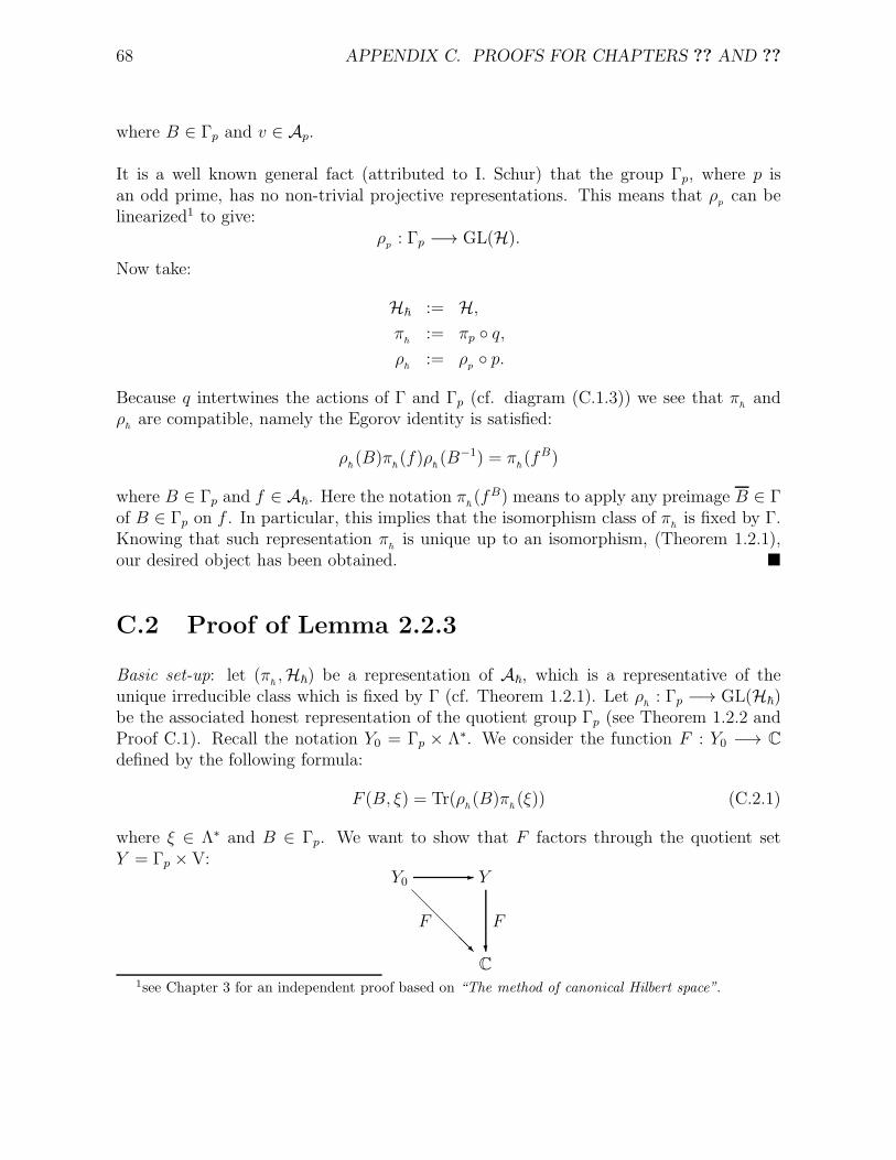
68 APPENDIX C. PROOFS FOR CHAPTERS ?? AND ??
where B ∈ Γp and v ∈ Ap.
It is a well known general fact (attributed to I. Schur) that the group Γp, where p isan odd prime, has no non-trivial projective representations. This means that ρp can belinearized1 to give:
ρp : Γp −→ GL(H).Now take:
H~ := H,π
~:= πp ◦ q,
ρ~
:= ρp ◦ p.
Because q intertwines the actions of Γ and Γp (cf. diagram (C.1.3)) we see that π~and
ρ~are compatible, namely the Egorov identity is satisfied:
ρ~(B)π
~(f)ρ
~(B−1) = π
~(fB)
where B ∈ Γp and f ∈ A~. Here the notation π~(fB) means to apply any preimage B ∈ Γ
of B ∈ Γp on f . In particular, this implies that the isomorphism class of π~is fixed by Γ.
Knowing that such representation π~is unique up to an isomorphism, (Theorem 1.2.1),
our desired object has been obtained. �
C.2 Proof of Lemma 2.2.3
Basic set-up: let (π~,H~) be a representation of A~, which is a representative of the
unique irreducible class which is fixed by Γ (cf. Theorem 1.2.1). Let ρ~: Γp −→ GL(H~)
be the associated honest representation of the quotient group Γp (see Theorem 1.2.2 andProof C.1). Recall the notation Y0 = Γp × Λ∗. We consider the function F : Y0 −→ C
defined by the following formula:
F (B, ξ) = Tr(ρ~(B)π
~(ξ)) (C.2.1)
where ξ ∈ Λ∗ and B ∈ Γp. We want to show that F factors through the quotient setY = Γp × V:
Y0 Y✲
F
❅❅❅❅❅❘
C❄
F
1see Chapter 3 for an independent proof based on “The method of canonical Hilbert space”.
C.3. PROOF OF THE GEOMETRIZATION THEOREM 69
The proof is immediate, taking into account the construction given in section C.1. Letπp be the unique (up to isomorphism) representation of the quotient algebra Ap. Aswas stated in C.1, π
~is isomorphic to πp ◦ q, where q : A~ −→ Ap is the quotient
homomorphism between the algebras. This means that π~(ξ) = πp(q(ξ)) depends only on
the image q(ξ) ∈ V, and formula (C.2.1) solves the problem. �
C.3 Proof of the Geometrization Theorem
Basic set-up: in this section we use the notations of section C.1 and Chapter 3. Set Y :=Spω×V and let α : Spω×Y −→ Y denotes the associated action map. Let F : Y −→ C bethe function appearing in the statement of Theorem 2.2.4, i.e., F (B, v) := Tr(ρp(B)πp(v)),where B ∈ Spω and v ∈ V. We use the notations V, Spω and Y to denote the correspond-ing algebraic varieties. For the convenience of the reader we repeat here the formulationof the statement:
Theorem 2.2.4 (Geometrization Theorem). There exists an object F ∈ Dbc,w(Y)satisfying the following properties:
1. (Function) fF = F .
2. (Weight) w(F) ≤ 0.
3. (Equivariance) For every element S ∈ Spω there exists an isomorphism α∗SF ≃ F .
4. (Formula) On introducing coordinates V ≃ A2 and identifying Spω ≃ SL2, thereexists an isomorphism
F|T×V≃ Lψ( 1
2λµ a+1
a−1) ⊗Lσ(a).
Here T = {(
a 00 a−1
)
} stands for the standard torus and (λ, µ) are the coordinates onV.
Construction of the sheaf F . We use the notations of Chapter 3. Let E be theHeisenberg group. As a set we have E = V×Fq. The group structure is given by the mul-tiplication rule (v, λ) · (v′, λ′) := (v + v′, λ+ λ′ + 1
2 ω(v, v′)). We fix a section s : V 99K E,
s(v) = (v, 0). The group of linear symplectomorphisms Spω acts on E by the formulag · (v, λ) := (gv, λ). Let D = Spω ⋉ E. We have a map Y −→ D defined using the sections. We use the notations E and D to denote the corresponding algebraic varieties.
Let K be the Weil representation sheaf (see Theorem 3.4.2). Define:
F := Tr(K|Y)
70 APPENDIX C. PROOFS FOR CHAPTERS ?? AND ??
where Tr is the trace functor (C.3.1).
We prove that F satisfies properties 1 - 4.
Property 1. The collection of operators {πp(v)}v∈V extends to a representation of thegroup E. The representation ρp ⋉ πp of the group D is isomorphic to the analogue repre-sentation ρ⋉ π constructed in Chapter 3. Hence:
fF = fTr(K|Y) = Tr(fK|Y ) = Tr(K|Y) =: F.
This proves Property 1.
Property 2. The sheaf K is of pure weight 0 (Corollary 3.4.3). The restriction tothe subvariety Y does not increase weight. The operation of Tr also does not increaseweight (using Theorem 2.2.5). It is defined as a composition:
Tr := pr1!∆1∗
12 (C.3.1)
where ∆112 : A
1 −→ A2 is the diagonal morphism ∆112(x) = (x, x) and pr1 is projection on
the Y coordinate:Y× A2
∆112
x
Y× A1
pr1
y
Y
Putting everything together we obtained Property 2.
Property 3. Basically follows from the convolution property of the sheaf K (see Theorem3.4.2 property 2). More precisely, using the convolution property we obtain the followingisomorphism:
K|S ∗ K ∗ K|S−1≃ L∗
SR∗S−1K
where LS, RS−1 denotes left multiplication by S and right multiplication by S−1 on thegroup D respectively. We write:
α∗SF ≃ Tr(α∗
SK|Y) ≃ Tr(L∗SR
∗S−1K|Y) ≃ Tr(K|S ∗ K|Y ∗ K|S−1
).
Now use the following facts:
Tr(K|S ∗ K|Y ∗ K|S−1) ≃ Tr(K|S−1
∗ K|S ∗ K|Y)
C.4. COMPUTATIONS FOR THE VANISHING LEMMA 71
and:
K|S−1∗ K|S ≃ I.
The first isomorphism is the basic tracial property. Its proof is completely formal and weomit it. The second isomorphism is a consequence of the convolution property of K. Thiscompletes the proof of Property 3.
Property 4. It is directly verified using the explicit formulas appearing in 3.3 whichare used to construct the sheaf K. More-precisely, we need to compute the formula forthe Trace of the Weil representation sheaf restricted to T r {I} × A2 × 0. We have:
F(a, λ, µ, 0) := Tr(K(a, λ, µ, 0)) = Lψ( 12λµ a+1
a−1) ⊗Lσ(a), a 6= 1.
Here Lσ is the Legendre character sheaf on Gm.
This completes the proof of the Geometrization Theorem. �
C.4 Computations for the Vanishing Lemma
In the computations we use some finer technical tools from the theory of ℓ-adic cohomol-ogy. The interested reader can find a systematic study of this material in [K, KW].
We identify the standard torus T ⊂ SL2 with the group Gm. Fix a non-trivial char-acter sheaf2 Lχ on Gm. Consider the variety X := Gm − {1}, the sheaf:
E := Lψ( 12λµ a+1
a−1) ⊗Lχ (C.4.1)
on X and the canonical projection pr : X −→ pt. Note that E is a non-trivial 1-dimensionallocal system on X. The proof of the Lemma will be given in several steps:
Step 1. Vanishing. We want to show that Hi(pr!E) = 0 for i = 0, 2.
By definition:
H0(pr!E) := Γ(Y, j!E)2Namely, a 1-dimensional local system on Gm that satisfies the property m∗Lχ ⋍ Lχ ⊠Lχ, where
m : Gm ×Gm −→ Gm is the multiplication morphism.
72 APPENDIX C. PROOFS FOR CHAPTERS ?? AND ??
where j : X → Y is the imbedding of X into a compact curve Y. The statement followssince:
Γ(Y, j!E) = Hom(Qℓ, j!E)and it is easy to see that any non-trivial morphism Qℓ −→ j!E should be an isomorphism,hence Hom(Qℓ, j!E) = 0.
For the second cohomology we have:
H2(pr!E) = H−2(Dpr!E)∗ = H−2(pr∗DE)∗ = Γ(X, DE [−2])∗
where D denotes the Verdier duality functor and [−2] means translation functor. Thefirst equality follows from the definition of D, the second equality is the Poincare dualityand the third equality easily follows from the definitions. Again, since the sheaf DE [−2]is a non-trivial 1-dimensional local system on X then:
Γ(X, DE [−2]) = Hom(Qℓ, DE [−2]) = 0.
Step 2. Dimension. We claim that dim H1(pr!E) = 2.
The (topological) Euler characteristic χ(pr!E) of the sheaf pr!E is the integer definedby the formula:
χ(pr!E) :=∑
i
(−1)idim Hi(pr!E).
Hence from the vanishing of cohomologies (Step 1) we deduce:
Substep 2.1. It is enough to show that χ(pr!E) = −2.
The actual computation of the Euler characteristic χ(pr!E) is done using theOgg-Shafarevich-
Grothendieck formula [D3]:
χ(pr!E)− χ(pr!Qℓ) =∑
y∈Y\XSwany(E) (C.4.2)
Where Qℓ denotes the constant sheaf on X, and Y is some compact curve containing X.In words, this formula expresses the difference of χ(pr!E) from χ(pr!Qℓ) as a sum of localcontributions.
Next, we take Y := P1. Having that χ(pr!Qℓ) = −1 and using formula (C.4.2) weget:
Substep 2.2. It is enough to show that: Swan0(E) + Swan1(E) + Swan∞(E) = −1.
C.4. COMPUTATIONS FOR THE VANISHING LEMMA 73
Now, using the explicit formula (C.4.1) of the sheaf E we see that:
Swan1(E) = Swan∞(Lψ),
Swan∞(E) = Swan∞(Lχ),
Swan0(E) = Swan0(Lχ).
Applying the Ogg-Shafarevich-Grothendieck formula to the Artin-Schreier sheaf Lψ onA1 and the projection pr : A1 −→ pt we find that:
Swan∞(Lψ) = χ(pr!Lψ)− χ(pr!Qℓ) = 0− 1 = −1. (C.4.3)
Finally we apply the formula (C.4.2) to the sheaf Lχ on Gm and the projection pr :Gm −→ pt and conclude:
Swan∞(Lχ) + Swan0(Lχ) = χ(pr!Lχ)− χ(pr!Qℓ) = 0− 0 = 0. (C.4.4)
In (C.4.3) and (C.4.4) we use the fact that pr!Lψ and pr!Lχ are the 0−objects in Dbc,w(pt).
This completes the computations of the Vanishing Lemma. �
Bibliography
[A] Auslander L., Kostant B. Quantization and representations of solvable Lie groups. Bull.Amer. Math. Soc. 73 (1967) 692-695.
[B] Bernstein J., private communication, Max-Planck Institute, Bonn, Germany (August,2004).
[BBD] Beilinson A. A., Bernstein J. and Deligne P. Faisceaux pervers. Analysis and topology onsingular spaces, I, Asterisque, 100, Soc. Math. France, Paris (1982), 5–171.
[BDB] Bouzouina A., De Bievre S., Equipartition of the eigenfunctions of quantized ergodicmaps on the torus. Commun.Math.Phys. 178 (1996), 83-105.
[BL] Bernstein J. and Lunts V., Equivariant sheaves and functors. Lecture Notes in Mathemat-ics, 1578. Springer-Verlag, Berlin (1994).
[CM] Coxeter H. S. M. and Moser, W. O. J., Generators and relations for discrete groups.Ergebnisse der Mathematik und ihrer Grenzgebiete, 14. Springer-Verlag, Berlin-New York(1980).
[D] Degli Esposti M., Quantization of the orientation preserving automorphisms of the torus.Ann. Inst. Henri Poincare 58 (1993), 323-341.
[D1] Deligne P., Metaplectique. A letter to Kazhdan (1982).
[D2] Deligne P., La conjecture de Weil II. Publ. Math. I.H.E.S 52 (1981), 313-428.
[D3] Deligne P., Raport sur la Formulae des traces. Cohomologie etale, Seminaire de GeometrieAlgebrique du Bois-Marie SGA 41
2 , Springer Lecture Notes in Mathematics 569 (1977),76-109.
[D4] Deligne P., Note on quantization. Quantum fields and strings: a course for mathematicians,Vol. 1, 2 (Princeton, NJ, 1996/1997), Amer. Math. Soc. Providence, RI (1999) 367–375.
[DGI] Degli Esposti M., Graffi S. and Isola S. Classical limit of the quantized hyperbolic toralautomorphisms. Comm. Math. Phys. 167 (1995), no. 3, 471–507.
74
BIBLIOGRAPHY 75
[G] Grothendieck A., Formule de Lefschetz et rationalite des fonctions L. Seminaire Bourbaki,Vol. 9, Exp. No. 279 (1964).
[Ga] Gaitsgory D., Informal introduction to geometric Langlands. An introduction to the Lang-lands program, Jerusalem 2001 , Birkhauser, Boston, MA (2003) 269-281.
[Ge] Gerardin P., Weil representations associated to finite fields. J. Algebra 46 (1977), no. 1,54-101.
[GH1] Gurevich S. and Hadani R., On Hannay-Berry Equivariant Quantization of the Torus.arXiv:math-ph/0312039.
[GH2] Gurevich S. and Hadani R., On Hannay-Berry Equivariant Quantization of Higher-dimesional Tori. arXiv:math-ph/0403036.
[GH3] Gurevich S. and Hadani R., Proof of the Kurlberg-Rudnick Rate Conjecture. arXiv:math-ph/0404074.
[GH4] Gurevich S. and Hadani R., The Higher-Dimensional Kurlberg-Rudnick Conjecture. Inpreparation.
[HB] Hannay J.H. and Berry M.V., Quantization of linear maps on the torus - Fresnel diffractionby a periodic grating. Physica D1 (1980), 267-291.
[K] Katz N.M., Gauss sums, Kloosterman sums and monodromy groups. Annals of Mathemat-ics Studies, 116. Princeton University Press, Princeton, NJ (1988).
[Ku] Kurlberg P., private communication, Chalmers University, Gothenburg, Sweden (Septem-ber, 2003).
[Ka] Kazhdan D., private communication, Hebrew University, Jerusalem, Israel (March, 2004).
[Ki] Kirillov A. A., Lectures on the orbit method. Graduate Studies in Mathematics, 64. Amer-ican Mathematical Society, Providence,RI (2004).
[Kl] Kloosterman H. D., ”The Behavior of General Theta Functions under the Modular Groupand the Characters of Binary Modular Congruence Groups, I.” Ann. Math. 47 (1946),317-375.
[KL] Katz N.M. and Laumon G., Transformation de Fourier et majoration de sommes expo-nentielles. Inst. Hautes Etudes Sci. Publ. Math. No. 62 (1985), 361-418.
[Ko] Kostant B., Quantization and unitary representations. Lecture Notes in Math., Vol. 170Springer, Berlin (1970) 87-208.
[KR1] Kurlberg P. and Rudnick Z., Hecke theory and equidistribution for the quantization oflinear maps of the torus. Duke Math. Jour. 103 (2000), 47-78.
76 BIBLIOGRAPHY
[KR2] Kurlberg P. and Rudnick Z., On the distribution of matrix elements for the quantum catmap. Annals of Mathematics, to appear.
[KW] Kiehl R. and Weissauer R., Weil conjectures, perverse sheaves and ℓ-adic Fourier trans-form. A Series of Modern Surveys in Mathematics, 42. Springer-Verlag, Berlin (2001).
[LV] Lion G. and Vergne M., The Weil representation, Maslov index and theta series. Progressin Mathematics, 6. Birkhauser, Boston, Mass. (1980).
[M] Milne J.S., Etale cohomology. Princeton Mathematical Series, 33. Princeton UniversityPress, Princeton, N.J. (1980).
[Me] F. Mezzadri, On the multiplicativity of quantum cat maps. Nonlinearity 15 (2002), 905-922.
[MR] McConnell J.C. and Robson J.C., Non-commutative Noetherian Rings. Graduate studiesin mathematics, 30. Amer. Math. Soc. Providence, RI (2001), 343-344.
[R1] Rudnick Z., The quantized cat map and quantum ergodicity. Lecture at the MSRI confer-ence ”Random Matrices and their Applications”, Berkeley, June 7-11, 1999.
[R2] Rudnick Z., On quantum unique ergodicity for linear maps of the torus. European Congressof Mathematics, Vol. II (Barcelona, 2000), Progr. Math., 202, Birkhauser, Basel (2001),429-437.
[Ri] Rieffel M.A., Non-commutative tori—a case study of non-commutative differentiable man-ifolds, Contemporary Math. 105 (1990), 191-211.
[S1] Sarnak P., private communication, Cambridge University, England (June, 2004).
[S2] Sarnak P., Arithmetic quantum chaos. The Schur lectures, 1992, Tel Aviv. Israel Math.Conf. Proc., 8, Bar-Ilan Univ., Ramat Gan (1995) 183-236.
[So] Souriau J.M., Structure des systemes dynamiques. Dunod, Paris (1970).
[V] Vogan D.A., The method of coadjoint orbits for real reductive groups. Representationtheory of Lie groups (Park City, UT, 1998) Amer. Math. Soc., Providence, RI (2000),179–238.
[W1] Weil A., Sur les courbes algebriques et les varietes qui s’en deduisent, Hermann et Cie.,Paris (1948).
[W2] Weil A., Sur certains groupes d’operateurs unitaires. Acta Math. 111 (1964) 143-211.