SIAM J. SCI. COMPUT. c© 2017 Society for Industrial and Applied MathematicsVol. 39, No. 5, pp. S610–S632

WEIGHTED INNER PRODUCTS FOR GMRES AND GMRES-DR∗

MARK EMBREE† , RONALD B. MORGAN‡ , AND HUY V. NGUYEN§

Abstract. The convergence of the restarted GMRES method can be significantly improved,for some problems, by using a weighted inner product that changes at each restart. How does thisweighting affect convergence, and when is it useful? We show that weighted inner products canhelp in two distinct ways: when the coefficient matrix has localized eigenvectors, weighting canallow restarted GMRES to focus on eigenvalues that otherwise cause slow convergence; for generalproblems, weighting can break the cyclic convergence pattern into which restarted GMRES oftensettles. The eigenvectors of matrices derived from differential equations are often not localized, thuslimiting the impact of weighting. For such problems, incorporating the discrete cosine transforminto the inner product can significantly improve GMRES convergence, giving a method we call W-GMRES-DCT. Integrating weighting with eigenvalue deflation via GMRES-DR can also give effectivesolutions.

Key words. linear equations, localized eigenvectors, weighted inner product, restarted GMRES,GMRES-DR, W-GMRES-DCT, deflation

AMS subject classifications. 65F10, 15A06

DOI. 10.1137/16M1082615

1. Introduction. We seek to solve large nonsymmetric systems of linear equa-tions using variants of the GMRES method [40] that change the inner product eachtime the method is restarted.

To solve Ax = b for the unknown x, GMRES computes the approximate solu-tion xk from the Krylov subspace Kk(A, b) = span{b, Ab, . . . , Ak−1b} that minimizesthe norm of the residual rk := b − Axk. This residual is usually optimized in the(Euclidean) 2-norm, but the algorithm can be implemented in any norm induced byan inner product. This generality has been studied in theory (see, e.g., [16, 17]) andin practice. The inner product affects neither the spectrum of A nor the subspaceKk(A, b) (assuming the method is not restarted), but it can significantly alter thedeparture of A from normality and the conditioning of the eigenvalues. Numerousauthors have proposed inner products in which certain preconditioned saddle pointsystems are self-adjoint, enabling optimal short-recurrence Krylov methods in placeof the long recurrences required for the 2-norm [7, 18, 26, 27, 45]. Recently Pestanaand Wathen used nonstandard inner products to inform preconditioner design [36].

For any inner product 〈·, ·〉W on Rn, there exists a matrix W ∈ Rn×n for which〈u, v〉W = v∗Wu for all u, v ∈ Rn, and W is Hermitian positive definite in the Eu-clidean inner product. (Throughout, ∗ denotes the conjugate transpose.) With theW -inner product is associated the norm ‖u‖W =

√〈u, u〉W =

√u∗Wu. To implement

∗Received by the editors July 1, 2016; accepted for publication (in revised form) April 10, 2017;published electronically October 26, 2017.

http://www.siam.org/journals/sisc/39-5/M108261.htmlFunding: The first author’s research was supported in part by National Science Foundation

grant DGE-1545362. The second author’s research was supported in part by the National ScienceFoundation Computational Mathematics Program under grant DMS-1418677.†Department of Mathematics and Computational Modeling and Data Analytics Division,

Academy of Integrated Science, Virginia Tech, Blacksburg, VA 24061 (embree@vt.edu).‡Department of Mathematics, Baylor University, Waco, TX 76798-7328 (Ronald Morgan@baylor.

edu).§Department of Mathematics and Computer Science, Austin College, Sherman, TX 75090

(hnguyen@austincollege.edu).

S610

WEIGHTED GMRES AND GMRES-DR S611

GMRES in the W -inner product, simply replace all norms and inner products in thestandard GMRES algorithm. Any advantage gained by this new geometry must bebalanced against the extra expense of computing the inner products: essentially onematrix-vector product with W for each inner product and norm evaluation.

In 1998 Essai proposed an intriguing way to utilize the inner product in restartedGMRES [14]: take W to be diagonal and change the inner product at each restart.His computational experiments show that this “weighting” can significantly improvethe performance of restarted GMRES, especially for difficult problems and frequentrestarts. Subsequent work has investigated how weighted GMRES performs on largeexamples [9, 23, 29, 33, 42]. We offer a new perspective on why weighting helps (ornot), justified by simple analysis and careful computational experiments.

Section 2 describes Essai’s algorithm. In section 3, we provide some basic analysisfor weighted GMRES and illustrative experiments, arguing that the algorithm per-forms well when the eigenvectors are localized. In section 4 we propose a new variantthat combines weighting with the discrete cosine transform, which localizes eigenvec-tors in many common situations. Section 5 describes a variant with deflated restarting(GMRES-DR [31]) that both solves linear equations and computes eigenvectors. Theeigenvectors improve the convergence of the solver for the linear equations, and aweighted inner product can help further.

2. Weighted GMRES. The standard restarted GMRES algorithm [40] com-putes the residual-minimizing approximation from a degree-m Krylov subspace andthen uses the residual associated with this solution estimate to generate a new Krylovsubspace. We call this algorithm GMRES(m) and every set of m iterations after arestart a cycle. Essai’s variant [14], which we call W-GMRES(m), changes the innerproduct at the beginning of each cycle of restarted GMRES, with weights determinedby the residual vector obtained from the last cycle. Let rkm = b − Axkm denotethe GMRES(m) residual after k cycles. Then the weight matrix defining the innerproduct for the next cycle is W = diag(w1, . . . , wn), where

(1) wj = max{|(rkm)j |‖rkm‖∞

, 10−10},

where (rkm)j denotes the jth entry of rkm.1 The weighted inner product is then〈u, v〉W = v∗Wu giving the norm ‖u‖W =

√〈u, u〉W . At the end of a cycle, the

residual vector rkm is computed and from it the inner product for the next cycle isbuilt. We have found it helpful to restrict the diagonal entries in (1) to be at least10−10, thus limiting the condition number of W to ‖W‖2‖W−1‖2 ≤ 1010. Finiteprecision arithmetic influences GMRES in nontrivial ways; see, e.g., [28, sect. 5.7].Weighted inner products can further complicate this behavior; a careful study of thisphenomenon is beyond the scope of our study, but note that Rozloznık et al. [37] havestudied orthogonalization algorithms in general inner products. (Although reorthog-onalization is generally not needed for GMRES [34], all tests here use one step of fullreorthogonalization for extra stability. Running the experiments in section 2 withoutthis step yields qualitatively similar results, but the iteration counts differ. All com-putations were performed using MATLAB 2015b. Different MATLAB versions yieldsomewhat different results, especially for experiments that require many iterations.)

For diagonal W , the inner product takes 3n operations (additions and multi-plications), instead of 2n for the Euclidean case. This increase of roughly 25% in

1Essai scales these entries differently, but, as Cao and Yu [9] note, scaling the inner product bya constant does not affect the residuals produced by the algorithm.

S612 MARK EMBREE, RONALD B. MORGAN, AND HUY V. NGUYEN

the Gram–Schmidt step in GMRES can be significant for very sparse A, but if thematrix-vector product is expensive, the cost of weighting is negligible.

How can weighting help? Suppose we restart GMRES every m iterations.GMRES minimizes a residual of the form ϕ(A)r, where ϕ is a polynomial of de-gree no greater than m with ϕ(0) = 1. When A is nearly normal, one learns muchfrom the magnitude of ϕ on the spectrum of A. Loosely speaking, since GMRES mustminimize the norm of the residual, the optimal ϕ cannot target isolated eigenvaluesnear the origin, since ϕ would then be large at other eigenvalues. This constraint cancause uniformly slow convergence from cycle to cycle; the restarted algorithm failsto match the “superlinear” convergence enabled by higher degree polynomials in fullGMRES [48]. (Higher degree polynomials can target a few critical eigenvalues witha few roots, while having sufficiently many roots remaining to be uniformly small onthe rest of the spectrum.) Weighting can skew the geometry to favor the trouble-some eigenvalues that impede convergence, leaving easy components to be eliminatedquickly in subsequent cycles. In aggregate, weighting can produce a string of iterates,each suboptimal in the 2-norm, that collectively give faster convergence than standardrestarted GMRES, with its locally optimal (but globally suboptimal) iterates.

Essai’s strategy for the inner product relies on the intuition that one should em-phasize those components of the residual vector that have the largest magnitude.Intuitively speaking, these components have thus far been neglected by the methodand may benefit from some preferential treatment. By analyzing the spectral proper-ties of the weighted GMRES algorithm in section 3, we explain when this intuition isvalid, show how it can go wrong, and offer a possible remedy.

Essai showed that his weighting can give significantly faster convergence for someproblems but did not provide guidance on matrix properties for which this was thecase. Later, Saberi Najafi and Zareamoghaddam [42] showed that diagonal W withentries from a random uniform distribution on [0.5, 1.5] can sometimes be effective,too. Weighting appears to be particularly useful when the GMRES(m) restart pa-rameter m is small, though it can help for larger m when the problem is difficult.

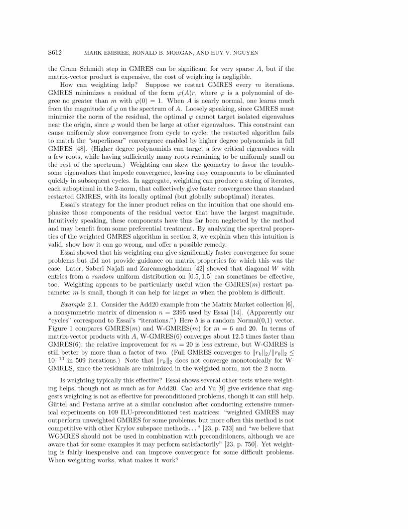
Example 2.1. Consider the Add20 example from the Matrix Market collection [6],a nonsymmetric matrix of dimension n = 2395 used by Essai [14]. (Apparently our“cycles” correspond to Essai’s “iterations.”) Here b is a random Normal(0,1) vector.Figure 1 compares GMRES(m) and W-GMRES(m) for m = 6 and 20. In terms ofmatrix-vector products with A, W-GMRES(6) converges about 12.5 times faster thanGMRES(6); the relative improvement for m = 20 is less extreme, but W-GMRES isstill better by more than a factor of two. (Full GMRES converges to ‖rk‖2/‖r0‖2 ≤10−10 in 509 iterations.) Note that ‖rk‖2 does not converge monotonically for W-GMRES, since the residuals are minimized in the weighted norm, not the 2-norm.

Is weighting typically this effective? Essai shows several other tests where weight-ing helps, though not as much as for Add20. Cao and Yu [9] give evidence that sug-gests weighting is not as effective for preconditioned problems, though it can still help.Guttel and Pestana arrive at a similar conclusion after conducting extensive numer-ical experiments on 109 ILU-preconditioned test matrices: “weighted GMRES mayoutperform unweighted GMRES for some problems, but more often this method is notcompetitive with other Krylov subspace methods. . . ” [23, p. 733] and “we believe thatWGMRES should not be used in combination with preconditioners, although we areaware that for some examples it may perform satisfactorily” [23, p. 750]. Yet weight-ing is fairly inexpensive and can improve convergence for some difficult problems.When weighting works, what makes it work?

WEIGHTED GMRES AND GMRES-DR S613

0 250 500 750 1000 1250 1500matrix{vector products with A

10 -10

10 -8

10 -6

10 -4

10 -2

10 0

krkk2

kr0k2

GMRES(6)

GMRES(20)

W-GMRES(6)

W-GM

RES(20)

fullGM

RES

Fig. 1. Convergence of full GMRES, GMRES(m), and W-GMRES(m) with m = 6 and m = 20for the Add20 matrix. In this and all subsequent illustrations, the residual norm is measured in thestandard 2-norm for all algorithms. Full GMRES converges to this tolerance in about 509 iterations.

3. Analysis of weighted GMRES. Analyzing W-GMRES(m) must be noeasier than analyzing standard restarted GMRES, an algorithm for which results arequite limited. (One knows conditions under which GMRES(m) converges for all initialresiduals [15] and about cyclic behavior for GMRES(n − 1) for Hermitian (or skew-Hermitian) A [4]. Few other rigorous results are known.) Restarted GMRES is anonlinear dynamical system involving the entries of A and b, and experiments suggestits convergence can depend sensitively on b [12]. Aware of these challenges, we seeksome insight by first studying a setting for which W-GMRES is ideally suited.

Let W = S∗S denote a positive definite matrix that induces the inner product〈u, v〉W = v∗Wu on Rn, with induced norm

‖u‖W =√〈u, u〉W =

√u∗Wu =

√u∗S∗Su = ‖Su‖2.

Given the initial guess x0 and residual r0 = b− Ax0, at the kth step GMRES in theW -inner product computes the residual rk that satisfies

‖rk‖W = minϕ∈Pk

ϕ(0)=1

‖ϕ(A)r0‖W = minϕ∈Pk

ϕ(0)=1

‖Sϕ(A)S−1Sr0‖2

= minϕ∈Pk

ϕ(0)=1

‖ϕ(SAS−1)Sr0‖2.

(Here Pk denotes the set of polynomials of degree k or less.) Thus, before any restartsare performed, W-GMRES applied to (A, r0) is equivalent to 2-norm GMRES appliedto (SAS−1, Sr0). (From this observation Guttel and Pestana propose an alternativeimplementation of W-GMRES, their Algorithm 2 [23, p. 744].) This connection be-tween W-GMRES and standard GMRES was first noted in an abstract by Gutknechtand Loher [22], who considered “preconditioning by similarity transformation.” SinceA and SAS−1 have a common spectrum, one expects full GMRES in the 2-norm andW -norm to have similar asymptotic convergence behavior. However, the choice ofS can significantly affect the departure of A from normality. For example, if A isdiagonalizable with A = V ΛV −1, then taking W = V −∗V −1 with S = V −1 rendersSAS−1 = Λ a diagonal (and hence normal) matrix.

S614 MARK EMBREE, RONALD B. MORGAN, AND HUY V. NGUYEN

The W -norms of the residuals produced by a cycle of W-GMRES will decreasemonotonically, but this need not be true of the 2-norms, as seen in Figure 1. In fact,

‖rk‖W = ‖Srk‖2 ≤ ‖S‖2‖rk‖2,

and similarly

‖rk‖2 = ‖S−1Srk‖2 ≤ ‖S−1‖2‖Srk‖2 = ‖S−1‖2‖rk‖W ,

so1‖S‖2

‖rk‖W ≤ ‖rk‖2 ≤ ‖S−1‖2‖rk‖W .

Pestana and Wathen [36, Thm. 4] show that the same bound holds when the residualin the middle of this inequality is replaced by the optimal 2-norm GMRES residual.That is, if r(W )

k and r(2)k denote the kth residuals from GMRES in the W -norm and

2-norm (both before any restart is performed, k ≤ m), then

1‖S‖2

‖r(W )k ‖W ≤ ‖r(2)k ‖2 ≤ ‖S

−1‖2‖r(W )k ‖W .

Thus for W -norm GMRES to depart significantly from 2-norm GMRES over thecourse of one cycle, S must be (at least somewhat) ill-conditioned. However, restart-ing with a new inner product can change the dynamics across cycles significantly.

3.1. The ideal setting for W-GMRES. For diagonal W , as in [14], let

S = diag(s1, . . . , sn) := W 1/2.

When the coefficient matrix A is diagonal,

A = diag(λ1, . . . , λn),

Essai’s weighting is well motivated and its effects can be readily understood.2 In thiscase, the eigenvectors are columns of the identity matrix, V = I, and SA = AS.Consider a cycle of W-GMRES(m) starting with r0 = b = [b1, . . . , bn]T . For k ≤ m,

‖rk‖2W = minϕ∈Pk

ϕ(0)=1

‖ϕ(A)b‖2W = minϕ∈Pk

ϕ(0)=1

‖Sϕ(A)b‖22(2a)

= minϕ∈Pk

ϕ(0)=1

‖ϕ(SAS−1)Sb‖22(2b)

= minϕ∈Pk

ϕ(0)=1

‖ϕ(A)Sb‖22 = minϕ∈Pk

ϕ(0)=1

n∑j=1

|ϕ(λj)|2|sjbj |2.(2c)

This last formula reveals that the weight sj affects GMRES in the same way as thecomponent bj of the right-hand side (which is the component of b in the jth eigenvectordirection for this A), so the weights tune how much GMRES will emphasize any giveneigenvalue. Up to scaling, Essai’s proposal amounts to sj =

√|bj |, so

(3) ‖rk‖2W = minϕ∈Pk

ϕ(0)=1

n∑j=1

|ϕ(λj)|2 |bj |3.

2Examples 1 and 2 of Guttel and Pestana [23] use diagonal A, and the analysis here can helpexplain their experimental results.

WEIGHTED GMRES AND GMRES-DR S615

This approach favors large components in b over smaller ones. Small entries in b(reduced at a previous cycle) were “easy” for GMRES to reduce because, for example,they correspond to eigenvalues far from the origin. Large entries in b have beenneglected by previous cycles, most likely because they correspond to eigenvalues nearthe origin. A low-degree polynomial that is small at these points is likely to be largeat large magnitude eigenvalues and so will not be picked as the optimal polynomial byrestarted GMRES. Weighting tips the scales to favor these neglected eigenvalues nearthe origin for one cycle; this preference will usually increase the residual in “easy”components, but such an increase can be quickly remedied at the next cycle. Considerhow standard GMRES(1) handles the scenario

0 < λ1 � 1 ≤ λ2 ≈ · · · ≈ λn.

Putting the root ζ of the residual polynomial ϕ(z) = 1 − z/ζ near the cluster ofeigenvalues λ2 ≈ · · · ≈ λn will significantly diminish the residual vector in components2, . . . , n, while not increasing the first component, since |ϕ(λ1)| < 1. On the otherhand, placing ζ near λ1 would give |ϕ(λj)| � 1 for j = 2, . . . , n, increasing the overallresidual norm, but in a manner that could be remedied at the next cycle if GMRES(1)could take a locally suboptimal cycle to accelerate the overall convergence. Essai’sweighting enables GMRES to target that small magnitude eigenvalue for one cycle,potentially at an increase to the 2-norm of the residual that can be corrected at thenext step without undoing the reduced component associated with λ1.

3.1.1. The diagonal case: Targeting small eigenvalues.

Example 3.1. Consider the diagonal matrix

A = diag(0.01, 0.1, 3, 4, 5, . . . , 9, 10).

Here b = r0 is a Normal(0,1) vector (MATLAB command randn with rng(1319)),scaled so ‖r0‖2 = 1. Figure 2 compares W-GMRES(m) to GMRES(m) for m = 3and m = 6: in both cases, weighting gives a big improvement. Figure 3 comparesconvergence of GMRES(3) and W-GMRES(3) for 5000 Normal(0,1) right-hand-sidevectors (also scaled so ‖r0‖2 = 1). As in Figure 2, W-GMRES(3) usually substantiallyimproves convergence, but it also adds considerable variation in performance. (Wehave noticed this tendency overall: weighting seems to add more variation, dependingon the right-hand side and finite-precision effects.)

0 50 100 150 200matrix{vector products with A

10 -8

10 -6

10 -4

10 -2

10 0

krkk2

kr0k2

GMRES(3)

W-G

MRES(3)

GM

RES(6)

W-G

MRES(6)

Fig. 2. GMRES(m) and W-GMRES(m) with m = 3, 6 for the diagonal test case, Example 3.1.

S616 MARK EMBREE, RONALD B. MORGAN, AND HUY V. NGUYEN

0

-2

-400

log10 krkk2

-650 -8

iteration, k

-10100

GMRES(3), 5000 trials

-12150

0.5

freq

uen

cy

1

0

-2

-400

log10 krkk2

-650 -8

iteration, k

-10100

W-GMRES(3), 5000 trials

-12150

0.5

freq

uen

cy

1

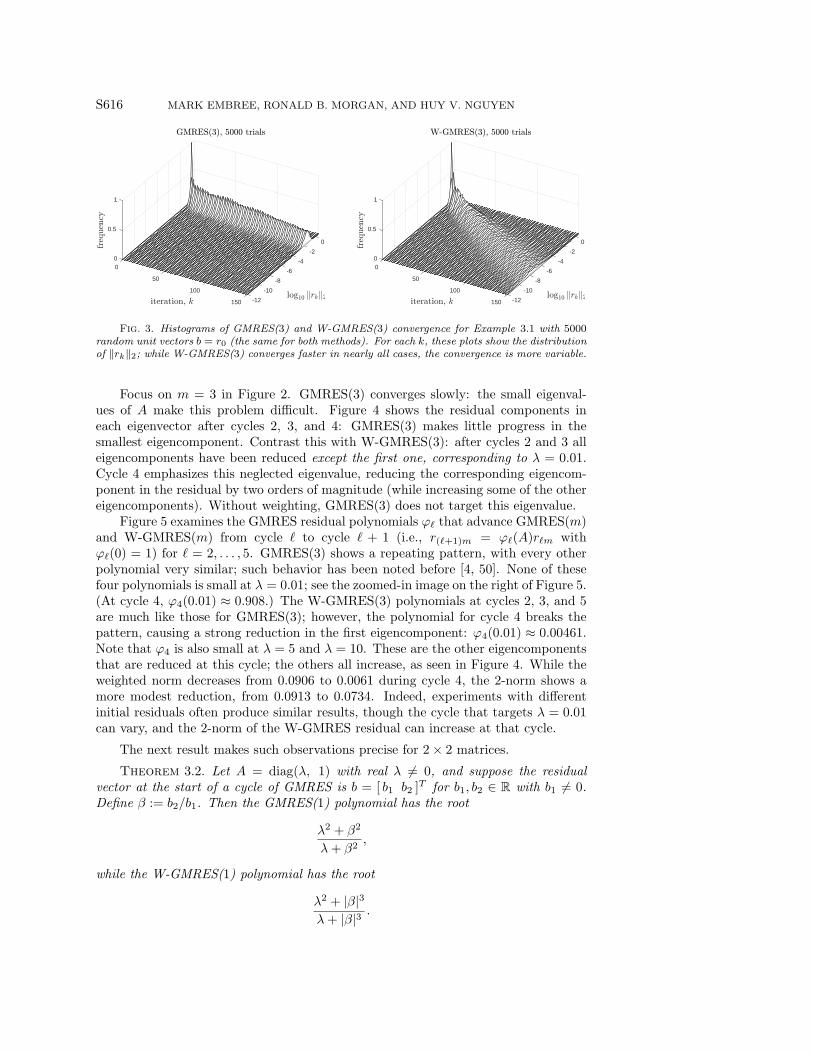
Fig. 3. Histograms of GMRES(3) and W-GMRES(3) convergence for Example 3.1 with 5000random unit vectors b = r0 (the same for both methods). For each k, these plots show the distributionof ‖rk‖2; while W-GMRES(3) converges faster in nearly all cases, the convergence is more variable.

Focus on m = 3 in Figure 2. GMRES(3) converges slowly: the small eigenval-ues of A make this problem difficult. Figure 4 shows the residual components ineach eigenvector after cycles 2, 3, and 4: GMRES(3) makes little progress in thesmallest eigencomponent. Contrast this with W-GMRES(3): after cycles 2 and 3 alleigencomponents have been reduced except the first one, corresponding to λ = 0.01.Cycle 4 emphasizes this neglected eigenvalue, reducing the corresponding eigencom-ponent in the residual by two orders of magnitude (while increasing some of the othereigencomponents). Without weighting, GMRES(3) does not target this eigenvalue.

Figure 5 examines the GMRES residual polynomials ϕ` that advance GMRES(m)and W-GMRES(m) from cycle ` to cycle ` + 1 (i.e., r(`+1)m = ϕ`(A)r`m withϕ`(0) = 1) for ` = 2, . . . , 5. GMRES(3) shows a repeating pattern, with every otherpolynomial very similar; such behavior has been noted before [4, 50]. None of thesefour polynomials is small at λ = 0.01; see the zoomed-in image on the right of Figure 5.(At cycle 4, ϕ4(0.01) ≈ 0.908.) The W-GMRES(3) polynomials at cycles 2, 3, and 5are much like those for GMRES(3); however, the polynomial for cycle 4 breaks thepattern, causing a strong reduction in the first eigencomponent: ϕ4(0.01) ≈ 0.00461.Note that ϕ4 is also small at λ = 5 and λ = 10. These are the other eigencomponentsthat are reduced at this cycle; the others all increase, as seen in Figure 4. While theweighted norm decreases from 0.0906 to 0.0061 during cycle 4, the 2-norm shows amore modest reduction, from 0.0913 to 0.0734. Indeed, experiments with differentinitial residuals often produce similar results, though the cycle that targets λ = 0.01can vary, and the 2-norm of the W-GMRES residual can increase at that cycle.

The next result makes such observations precise for 2× 2 matrices.

Theorem 3.2. Let A = diag(λ, 1) with real λ 6= 0, and suppose the residualvector at the start of a cycle of GMRES is b = [ b1 b2 ]T for b1, b2 ∈ R with b1 6= 0.Define β := b2/b1. Then the GMRES(1) polynomial has the root

λ2 + β2

λ+ β2 ,

while the W-GMRES(1) polynomial has the root

λ2 + |β|3

λ+ |β|3.

WEIGHTED GMRES AND GMRES-DR S617

1 2 3 4 5 6 7 8 9 10eigencomponent index, j

10 -8

10 -6

10 -4

10 -2

10 0

10 2

magnitude

ofjt

hei

gen

com

ponen

tofre

sidual

234 23

42

3

42

34

2

34

2

34

2

34

2

34

2

34

2

34

GMRES(3)

6

λ = 0.01

1 2 3 4 5 6 7 8 9 10eigencomponent index, j

10 -8

10 -6

10 -4

10 -2

10 0

10 2

magnitude

ofjt

hei

gen

com

ponen

tofre

sidual

23

423

4

23

4

23

4 23

4

2

3

4 2

3

4

2

3

4

2

3

423

4

W-GMRES(3)

6

λ = 0.01

Fig. 4. Eigencomponents of the residual at the end of cycles ` = 2, 3, and 4 for standardGMRES(3) (top) and W-GMRES(3) (bottom) applied to the matrix in Example 3.1. Cycle 4 ofW-GMRES(3) reduces the eigencomponent corresponding to λ1 = 0.01 by two orders of magnitude.

The proof is a straightforward calculation. To appreciate this theorem, take λ =β = 0.1, giving the roots 0.1818 for GMRES(1) and 0.1089 for W-GMRES(1). Thesepolynomials cut the residual component corresponding to λ = 0.1 by a factor 0.450 forGMRES(1) and 0.0818 for W-GMRES(1), the latter causing W-GMRES(1) to increasethe component for λ = 1 by a factor of 8.18. This increase is worthwhile, given thereduction in the tough small component; later cycles will handle the easier component.For another example, take λ = β = 0.01: GMRES(1) reduces the λ = 0.01 componentby 0.495, while W-GMRES(1) reduces it by 0.0098, two orders of magnitude.

3.1.2. The diagonal case: Breaking patterns in residual polynomials.Beyond the potential to target small eigenvalues, W-GMRES can also break the cyclicpattern into which GMRES(m) residual polynomials often lapse. Baker, Jessup, andManteuffel [4, Thm. 2] prove that if A is an n × n symmetric (or skew-symmetric)matrix, then the GMRES(n − 1) residual vectors exactly alternate in direction, i.e.,the residual vector at the end of a cycle is an exact multiple of the residual twocycles before; thus the GMRES residual polynomial at the end of each cycle repeatsthe same polynomial found two cycles before. Baker, Jessup, and Manteuffel observethe same qualitative behavior for more frequent restarts and suggest that disrupting

S618 MARK EMBREE, RONALD B. MORGAN, AND HUY V. NGUYEN

0 3 4 5 6 7 8 9 10z

-100

-80

-60

-40

-20

0

20

40

60

80

100

j'`(

z)j cycles 3, 5

cycles 2, 4

GMRES(3)

0 0.05 0.1 0.15z

-10

-8

-6

-4

-2

0

1

2 cycles 3, 5

cycles 2, 4

GMRES(3), zoom

0 3 4 5 6 7 8 9 10z

-100

-80

-60

-40

-20

0

20

40

60

80

100

j'`(

z)j cycles 3, 5

cycle 2

cycle4

W-GMRES(3)

0 0.05 0.1 0.15z

-10

-8

-6

-4

-2

0

1

2 cycles 3, 5

cycle 2cycle

4

W-GMRES(3), zoom

Fig. 5. Residual polynomials for cycles 2–5 of standard GMRES(3) (top) and W-GMRES(3)(bottom) for Example 3.1. The gray vertical lines show the eigenvalues of A. At cycle 4, the weightedinner product allows W-GMRES(3) to target the first eigencomponent, increasing other components.

this pattern (by varying the restart parameter [3] or augmenting the subspace [4])can improve convergence. (Longer cyclic patterns can emerge for nonnormal A [50].)Changing the inner product can have a similar effect, with the added advantageof targeting difficult eigenvalues if the corresponding eigenvectors are well-disposed.While Essai’s residual-based weighting can break cyclic patterns, other schemes (suchas random weighting [23, 42]; see subsection 3.5) can have a similar effect; however,such arbitrary inner products take no advantage of eigenvector structure. The nextexample cleanly illustrates how W-GMRES can break patterns.

Example 3.3. Apply GMRES(1) to A = diag(2, 1) with b = [ 1 1 ]T . The roots ofthe (linear) GMRES(1) residual polynomials alternate between 5/3 and 4/3 (exactly),as given by Theorem 3.2. Therefore the GMRES(1) residual polynomials for the cyclesalternate between ϕk(z) = 1− (3/5)z and ϕk(z) = 1− (3/4)z. GMRES(1) converges(‖rk‖2/‖r0‖2 ≤ 10−8) in 16 iterations. W-GMRES(1) takes only 7 iterations. AsFigure 6 shows, weighting breaks the cycle of polynomial roots, giving 1.667, 1.200,1.941, 1.0039, 1.999985, 1.0000000002, and ≈ 2: the roots move out toward theeigenvalues, alternating which eigenvalue they favor and reducing ‖rk‖2 much faster.

3.2. Measuring eigenvector localization. The justification for W-GMRESin (2c) required diagonal A, so the eigenvectors are columns of the identity matrix.When A is not diagonal, the motivation for W-GMRES is less compelling. Yet inmany applications A is not close to diagonal but still has localized eigenvectors: onlya few entries are large, and the eigenvectors resemble columns of the identity matrix.Computational evidence suggests that W-GMRES can still be effective, particularly

WEIGHTED GMRES AND GMRES-DR S619

1 2 3 4 5 6 7 8 9 10 11 12 13 14 15 16k

1

4/3

5/3

2GMRES(1)

1 2 3 4 5 6 7k

1

4/3

5/3

2W-GMRES(1)

Fig. 6. Roots of the GMRES(1) and W-GMRES(1) residual polynomials for A = diag(2, 1)with b = [1, 1]T , as a function of the restarted GMRES cycle, k. The GMRES(1) roots occur in arepeating pair, and the method takes 16 iterations to converge to ‖rk‖2/‖r0‖2 ≤ 10−8. In contrast,the W-GMRES(1) roots are quickly attracted to the eigenvalues, giving convergence in just 7 steps.

0 10 20 30 40p

0

0.2

0.4

0.6

0.8

1

loc p

(A)

Add20

2d Laplacian

Orsirr 1

Sherman5

matrix n loc5(A)Add20 2395 0.9996Orsirr 1 1030 0.3253Sherman5 3312 0.16762d Laplacian 9801 0.0475

Fig. 7. The localization measures locp(A) for p = 1, . . . , 40 for four matrices that are usedin our W-GMRES experiments. If locp(A) is close to 1, the eigenvectors associated with smallestmagnitude eigenvalues are highly localized.

when the eigenvectors associated with the small magnitude eigenvalues are localized.The Add20 matrix in Example 2.1 is such an example.

We gauge the localization of the p smallest magnitude eigenvectors by measuringhow much they are concentrated in their p largest magnitude entries.3 For diagonal-izable A, label the eigenvalues in increasing magnitude, |λ1| ≤ |λ2| ≤ · · · ≤ |λn|, withassociated unit 2-norm eigenvectors v1, . . . , vn. For any y ∈ Cn, let y(p) ∈ Cp denotethe subvector containing the p largest magnitude entries of y (in any order). Then

(4) locp(A) :=1√p

(p∑

j=1

‖v(p)j ‖

22

)1/2

.

Notice that locp(A) ∈ (0, 1], and locn(A) = 1. If locp(A) ≈ 1 for some p � n,the eigenvectors associated with the p smallest magnitude eigenvalues are localizedwithin p positions. This measure is imperfect, for it includes neither the magnitude ofthe eigenvalues nor the potential nonorthogonality of the eigenvectors. Still locp(A)can be a helpful instrument for assessing localization. Figure 7 shows locp(A) for

3Certain applications motivate more specialized measures of localization based on the rate ofexponential decay of eigenvector entries about some central entry.

S620 MARK EMBREE, RONALD B. MORGAN, AND HUY V. NGUYEN

p = 1, . . . , 40 for four matrices we use in our experiments.4 The Add20 matrix hasstrongly localized eigenvectors; the discrete 2d Laplacian has eigenvectors that arefar from localized; i.e., they are global. The Orsirr 1 and Sherman5 matrices haveeigenvectors with intermediate localization.

3.3. The nondiagonal case. When A is not diagonal, the justification for W-GMRES in (2c) is lost; the effect of weighting becomes more subtle. The weights canstill break cyclic patterns in restarted GMRES, but the interplay between the weightsand the eigenvectors is more difficult to understand. Suppose A is diagonalizable,A = V ΛV −1, still with W = S∗S. Unlike the diagonal case, S will not generallycommute with V and Λ, so (2) is replaced by

‖rk‖W = minϕ∈Pk

ϕ(0)=1

‖ϕ(SAS−1)Sb‖2(5a)

= minϕ∈Pk

ϕ(0)=1

‖(SV )ϕ(Λ)(SV )−1Sb‖2.(5b)

The matrix S transforms the eigenvectors of A [22]. Suppose, impractically, that V −1

were known, allowing the nondiagonal weight

S = diag(s1, . . . , sn)V −1.

In this case (5b) reduces to

(6) ‖rk‖2W = minϕ∈Pk

ϕ(0)=1

n∑j=1

|ϕ(λj)|2|sjbj |2 (eigenvector weighting)

a perfect analogue of the diagonal case (2c) that could appropriately target the smallmagnitude eigenvalues that delay convergence. One might approximate this eigenvec-tor weighting by using, as a proxy for V −1, some estimate of the left eigenvectors ofA associated with the smallest magnitude eigenvectors. (The rows of V −1 are the lefteigenvectors of A, since V −1A = ΛV −1.) We do not pursue this idea here, insteadusing eigenvector information via deflated restarting in section 5.

The conventional W-GMRES(m) algorithm instead uses diagonal W (and S).In this case, SV scales the rows of V , effectively emphasizing certain entries of theeigenvectors at the expense of others. Write out the right and left eigenvectors,

V = [v1 v2 · · · vn] ∈ Cn×n, V −1 =

v∗1v∗2...v∗n

∈ Cn×n.

Let c := V −1b denote the expansion coefficients for b in the eigenvectors of A: b = V c.Then one can also render (5b) in the form

(7) ‖rk‖W = minϕ∈Pk

ϕ(0)=1

∥∥∥∥∥n∑

j=1

cj ϕ(λj)Svj

∥∥∥∥∥2

(diagonal weighting)

4Two of these matrices, Sherman5 and the 2d Laplacian, have repeated (derogatory) eigenvalues;according to the principle of reachable invariant subspaces (see, e.g., [5, 28]), the GMRES processonly acts upon one eigenvector in the invariant subspace, given by the component of the initialresidual in that space. Thus the localization measures in Figure 7 include only one eigenvector forthe derogatory eigenvalues, specified by the initial residual vectors used in our experiments.

WEIGHTED GMRES AND GMRES-DR S621

a different analogue of (2c). Denote the `th entry of vj by (vj)`. In most cases V willbe dense. Suppose that only the qth entry of r0 is large, and that (vj)q 6= 0 for j =1, . . . , n. Then Essai’s weighting makes |(Svj)q| � |(Svj)`| for all ` 6= q: all the vectorsSvj form a small angle with the qth column of the identity. Thus SV is ill-conditionedand SAS−1 will have a large departure from normality, often a troublesome case forGMRES; see, e.g., [47, Chap. 26]. It is not evident how such weighting could helpW-GMRES(m) focus on small eigenvalues, as it does for diagonal A, suggesting anexplanation for the mixed performance of W-GMRES(m) [9, 23].

3.3.1. Stagnation of W-GMRES(m) when GMRES(m) converges. Weshow that by transforming the eigenvectors, diagonal weighting can even prevent W-GMRES(m) from converging at all. Faber et al. [15] prove that GMRES(m) convergesfor all initial residuals provided there exists no v ∈ Cn such that

v∗Akv = 0 for all k = 1, . . . ,m.

Thus GMRES(m) will converge for all m ≥ 1 and r0 if the field of values of A,

F (A) := {v∗Av : v ∈ Cn, ‖v‖2 = 1},

does not contain the origin. Weighting effectively applies GMRES to the transformedmatrix SAS−1, and now it is possible that 0 ∈ F (SAS−1) even though 0 6∈ F (A). Inextreme cases this means that W-GMRES(m) can stagnate even when GMRES(m)converges, as shown by the next example. (In contrast, for A and S diagonal,SAS−1 = A, so F (A) = F (SAS−1).)

Example 3.4 (W-GMRES(1) stagnates while GMRES(1) converges). Consider

(8) A =[

1 −40 5

], r0 =

[1

110 (5 +

√5)

]=[

10.72360 . . .

].

Figure 8 shows F (A), an ellipse in the complex plane. From the extreme eigenvalues ofthe Hermitian and skew-Hermitian parts of A, one can bound F (A) within a rectanglein C that does not contain the origin,

Re(F (A)) = [3− 2√

2, 3 + 2√

2] ≈ [0.17157, 5.82843], Im(F (A)) = [−2i, 2i],

0 1 2 3 4 5 6

-2

-1

0

1

2

F (A)

F (SAS!1 )

Fig. 8. The fields of values F (A) (gray region) and F (SAS−1) (boundary is a black line) in Cfor A and r0 in (8); the cross (+) marks the origin. Since 0 6∈ F (A), GMRES(m) converges for anyr0; however, 0 ∈ F (SAS−1) and (Sr0)∗(SAS−1)(Sr0) = 0, so W-GMRES(1) completely stagnates.

S622 MARK EMBREE, RONALD B. MORGAN, AND HUY V. NGUYEN

and hence GMRES(1) converges for all initial residuals. Now consider the specific r0given in (8). Using the scaling S = diag(

√|(r0)1|/‖r0‖∞,

√|(r0)2|/‖r0‖∞) at the first

step gives the W-GMRES(1) polynomial (see, e.g., [12, eq. (2.2)])

r1 = ϕ(A)r0 = r0 −(Sr0)∗(SAS−1)(Sr0)‖(SAS−1)(Sr0)‖22

(SAS−1)(Sr0) = r0 −r∗0S

2Ar0‖SAr0‖22

SAr0.

This example has been engineered so that 0 ∈ F (SAS−1); indeed,

Re(F (SAS−1)) =[3−

√14− 2

√5, 3 +

√14− 2

√5]≈ [−0.086724, 6.08672],

as seen in Figure 8. Worse still, this r0 gives r∗0S2Ar0 = 0, so r1 = r0: W-GMRES(1)

makes no progress, and the same weight is chosen for the next cycle. The weightedalgorithm completely stagnates, even though GMRES(1) converges for any r0.

3.3.2. Poor performance when small eigenvalues have global eigenvec-tors. The last example shows one way GMRES(m) can outperform W-GMRES(m)when A is not diagonal. Next we show that global eigenvectors associated with smallmagnitude eigenvalues can also contribute to poor W-GMRES(m) convergence.

Example 3.5 (W-GMRES(m) worse than GMRES(m): Global eigenvectors). Werevisit Example 3.1, again with dimension n = 10 and eigenvalues

Λ = diag(0.01, 0.1, 3, 4, 5, . . . , 9, 10),

but now let the eigenvectors of A equal those of the symmetric tridiagonal matrixtridiag(−1, 0,−1), ordering the eigenvalues from smallest to largest. (The jth col-umn of V has entries (vj)` = sin(j`π/(n + 1))/‖vj‖2; see, e.g., [44].) The resultingA = V ΛV ∗ is symmetric, unitarily similar to Λ. Let b be the same Normal(0,1) vec-tor used in Example 3.1. Since V is unitary, GMRES(m) applied to (Λ, b) producesthe same residual norms as GMRES(m) applied to (V ΛV ∗, V b). However, weightedGMRES can behave very differently for the two problems: when applied to Λ (as inExample 3.1), W-GMRES(6) vastly outperforms GMRES(6). For A with its nonlo-calized eigenvectors, W-GMRES(6) converges much more slowly, as seen in Figure 9.

0 50 100 150 200 250 300 350 400 450matrix{vector products with A

10 -8

10 -6

10 -4

10 -2

10 0

krkk2

kr0k2

GM

RES(6)

W-G

MRES(6)

on$

W-GMRES(6) on A

Fig. 9. GMRES(6) and W-GMRES(6) for Example 3.5. Applying GMRES(6) to (Λ, b) and(A, V b) produces identical residual 2-norms. When applied to (Λ, b), W-GMRES(6) converges fasterthan GMRES(6) (seen previously in Figure 2); when applied to (A, V b) the convergence is muchslower (A having nonlocalized eigenvectors).

WEIGHTED GMRES AND GMRES-DR S623

0 1000 2000 3000 4000 5000 6000 7000 8000 9000matrix{vector products with A

10 -6

10 -4

10 -2

10 0

krkk2

kr0k2

W-GMRES(30)

GMRES(30)

W-GMRES(100)

GMRES(100)

0 1000 2000 3000 4000 5000 6000 7000 8000 9000matrix{vector products with $

10 -8

10 -6

10 -4

10 -2

10 0

10 2

krkk2

kr0k2

GMRES(30)

GMRES(100)

W-GMRES(30)W-GMRES(100)

Fig. 10. GMRES(m) and W-GMRES(m) for the Sherman5 matrix. On the top, the methodsare applied to Ax = b, and weighting slows convergence. On the bottom, the same methods areapplied to Λx = b, where Λ is diagonal with the same eigenvalues of A; W-GMRES convergesbetter. (The GMRES(100) curve is yellow. Color is available online only.) For both problems,taking m = 100 steps with each weighted inner product gives large growth in ‖rk‖2 between restarts.

The next example shows similar behavior for a larger matrix: eigenvalues on bothsides of the origin and global eigenvectors give poor W-GMRES(m) performance.

Example 3.6 (W-GMRES(m) slower than GMRES(m): Global eigenvectors).Consider the nonsymmetric Sherman5 matrix from Matrix Market [6], with n = 3312and with r0 a Normal(0,1) vector. Figure 10 shows that weighting slows restartedGMRES, particularly for the restart m = 100. Figure 7 shows that the eigenvectorsare poorly localized; e.g., in the unit eigenvector v1 corresponding to the smallesteigenvalue, the 100 largest components range only from 0.0509 to 0.0415 in magnitude.This matrix has eigenvalues to the left and right of the origin, and the eigenvectorsare not orthogonal.5 The second plot in Figure 10 shows how the performance of W-GMRES improves when A is replaced by a diagonal matrix with the same spectrum.

3.3.3. Weighting sometimes helps despite global eigenvectors. The pastthree examples suggest that W-GMRES performs poorly for matrices whose eigenvec-tors are not localized, but the algorithm is more nuanced than that. The next example

5The eigenvalue λ = 1 has multiplicity 1674, and the corresponding eigenvectors are columns ofthe identity. The eigenvalues closest to the origin are well-conditioned, while some eigenvalues farfrom the origin are relatively ill-conditioned. (For the diagonalization computed by the MATLABcommand eig, ‖V ‖2‖V −1‖2 ≈ 3.237×106.) The pseudospectra of this matrix are well-behaved nearthe origin; the effect of the eigenvalue conditioning on GMRES convergence is mild [47, Chap. 26].

S624 MARK EMBREE, RONALD B. MORGAN, AND HUY V. NGUYEN

0 500 1000 1500 2000 2500 3000matrix{vector products with A

10 -8

10 -6

10 -4

10 -2

10 0

krkk2

kr0k2

GMRES(10)W-GMRES(10)

GMRES(20)

W-G

MRES(20)

Fig. 11. GMRES(m) and W-GMRES(m) for a discretization of the Dirichlet Laplacian on theunit square. The eigenvectors are not localized, but weighting still accelerates convergence.

is characteristic of behavior we have often observed in our experiments. We attributethe improvement over standard restarted GMRES to the tendency of weighting tobreak cyclic patterns in the GMRES residual polynomials.

Example 3.7 (W-GMRES(m) better than GMRES(m): Global eigenvectors).Consider the standard 5-point finite difference discretization of the Laplacian on theunit square in two dimensions with Dirichlet boundary conditions. The uniform gridspacing h = 1/100 in both directions gives a matrix of order n = 992 = 9801; theinitial residual is a random Normal(0,1) vector. The small locp(A) values shown inFigure 7 confirm that the eigenvectors are not localized; in fact, they are less localizedthan for the Sherman5 matrix in the last example. Despite this, Figure 11 shows thatW-GMRES(m) outperforms GMRES(m) for m = 10 and m = 20. In this case, allthe eigenvalues are positive, and none is particularly close to the origin.

3.4. Extra weighting. If weighting can improve GMRES, especially when thesmallest eigenvalues have localized eigenvectors, might more extreme weighting helpeven more? Recall from (2) that for diagonal A,

(9) ‖rk‖2W = minϕ∈Pk

ϕ(0)=1

n∑j=1

|ϕ(λj)|2|sjbj |2.

Essai’s standard weighting uses s2j = wj = |bj |. Suppose one instead takes s2j = wj =|bj |p for p ≥ 0. For large p we find it particularly important to limit the minimalweight, as in (1); we require wj ∈ [10−10, 1].

For most cases we have studied, extra weighting has little qualitative impact. Fordiagonal A, p > 1 can accelerate convergence; for the general case, even with localizedeigenvectors, results are mixed. The next example shows a case where it helps.

Example 3.8 (extra weighting, localized eigenvectors). The Orsirr 1 matrix fromMatrix Market [6] is a nonsymmetric matrix of dimension n = 1030. Figure 7 showsthe eigenvectors to be fairly well localized; all the eigenvalues are real and negative.Table 1 reports the matrix-vectors products (with A) required by W-GMRES(m) withdifferent weighting powers p to satisfy the convergence criterion ‖rk‖2/‖r0‖2 ≤ 10−8.(Here r0 is a random Normal(0,1) vector.) When m is small (e.g., m = 5 and 10),

WEIGHTED GMRES AND GMRES-DR S625

Table 1W-GMRES(m) for the Orsirr 1 matrix, with extra weighting by the power p. The table shows

the matrix-vector products with A required to reduce ‖rk‖2/‖r0‖2 by a factor of 10−8.

p 0 1 2 3 4 5 6 8 10m = 5 20000 20000 13854 8126 6641 7640 4043 3947 4512m = 10 16299 13883 5009 5901 3810 3198 3053 3129 3064m = 20 13653 2934 2569 2134 2221 2154 2303 2294 2377m = 30 3750 2572 2224 2012 2075 2009 1998 1961 2094

extra weighting improves convergence significantly. For example, when m = 10, thevalue p = 6 gives the best result among the reported p. For larger m, extra weightinghas less impact.

3.5. Random weighting. We have argued that when A has local eigenvectors,residual-based weighting can encourage convergence in certain eigenvector directionsand break repetitive patterns in GMRES(m). In contrast, when the eigenvectorsare predominantly global, weighting can still sometimes help by breaking patterns inGMRES(m), but there is no compelling connection to the eigenvectors. Thus if theeigenvectors of A are global, residual-based weighting should fare no better than therandom diagonal weighting proposed by Saberi Najafi and Zareamoghaddam [42]. Incontrast, for localized eigenvectors, residual-based weighting should have a significantadvantage over random weighting. The next two examples show this behavior.

Example 3.9 (random weights for a matrix with local eigenvectors). The Add20matrix from Example 2.1 has localized eigenvectors, and W-GMRES(m) improvedconvergence for m = 3 and m = 6. Table 2 compares this performance to two randomweighting schemes: W is a diagonal matrix with uniform random entries chosen inthe interval [0.5, 1.5] (first method) and [0, 1] (second method), with fresh weightsgenerated at each restart. All experiments use the same r0 as in Figure 1; sinceperformance changes for each run with random weights, we average the matrix-vectorproducts with A (iteration counts) over 10 trials each. All three weighted methodsbeat GMRES(m), but the residual-based weighting has a significant advantage.

Example 3.10 (random weights for a matrix with global eigenvectors). The re-sults are very different for the discretization of the Dirichlet Laplacian on the unitsquare (Example 3.7). Table 3 shows that residual-based weighting is inferior to mostof the random weighting experiments, with particularly extreme differences for smallm. There appears to be no advantage to correlating weighting to residual components.(This example shows a “tortoise and hare” effect [12], where the random weightingwith m = 1 often converges in fewer iterations than the larger m here.)

4. W-GMRES-DCT: Localizing eigenvectors with Fourier transforms.Equation (6) suggests that, for diagonalizableA = V ΛV −1, the ideal weighting schemeshould incorporate eigenvector information. It will be convenient to now express Win the form W = Z∗Z with Z = SV −1 for S = diag(s1, . . . , sn), giving

‖rk‖2W = minϕ∈Pk

ϕ(0)=1

n∑j=1

|ϕ(λj)|2|sjbj |2.

Incorporating V −1 into the weighting diagonalizes the problem and makes residualweighting compelling, but such an inner product is clearly impractical. However, we

S626 MARK EMBREE, RONALD B. MORGAN, AND HUY V. NGUYEN

Table 2For the Add20 matrix, the matrix-vector products (with A) required to converge to

‖rk‖2/‖r0‖2 ≤ 10−8 for GMRES(m) and W-GMRES(m), and random weights chosen uniformly in[0.5, 1.5] and [0, 1]. The random counts are averaged over 10 trials (same r0). W-GMRES(m) doesmuch better than the random schemes for this matrix with local eigenvectors.

m GMRES(m) W-GMRES(m) rand(.5,1.5) rand(0,1)1 > 20000 1785 15845.5 4077.12 > 20000 2882 10506.7 8190.23 > 20000 4580 8664.0 7237.16 10032 1022 4270.7 3382.7

10 4220 762 1945.4 1331.915 2469 716 1531.6 1126.820 1605 650 1109.1 1022.5

Table 3For the discrete Laplacian on the unit square, the matrix-vector products (with A) required

to converge to ‖rk‖2/‖r0‖2 ≤ 10−8 for GMRES(m), W-GMRES(m), and two random schemes:weights chosen uniformly in [0.5, 1.5] and [0, 1]. The random counts are averaged over 10 trials, allwith the same r0. For smaller values of m, the residual-based weighting of W-GMRES(m) performssignificantly worse than the random weighting for this matrix with global eigenvectors.

m GMRES(m) W-GMRES(m) rand(.5,1.5) rand(0,1)1 > 20000 > 20000 1446.0 1059.42 14449 9958 2499.8 2318.43 9687 6450 2670.6 2329.86 4867 3704 2267.1 1804.0

10 2912 2054 1726.3 1545.715 2017 1650 1742.0 1549.320 1556 1225 1404.1 1338.2

have seen that weighting can improve GMRES convergence if the eigenvectors aremerely localized. This suggests a new weighting strategy that uses W = Z∗Z with

Z = SQ∗, S = diag(s1, . . . , sn),

where Q is unitary and the weights s1, . . . , sn are derived from the residual as before.Since GMRES on (A, b) in this W -inner product amounts to standard 2-norm GMRESon (ZAZ−1, Zb) = (SQ∗AQS−1, SQ∗b), we seek Q in which the eigenvectors of Q∗AQare localized. When A is a discretization of a constant-coefficient differential operator,a natural choice for Q∗ is the discrete cosine transform matrix [46],6 since for manysuch problems the eigenvectors associated with the smallest-magnitude eigenvalues arelow in frequency. We call the resulting algorithm W-GMRES-DCT(m). In MATLAB,one could compute Q∗ = dct(eye(n)), a unitary but dense matrix that should neverbe formed; instead, it can be applied to vectors in O(n log n) time using the fastFourier transform. In MATLAB code, the inner product becomes

〈x, y〉W = y∗QS∗SQ∗x = (SQ∗y)∗(SQ∗x) = (s.*dct(y))’*(s.*dct(x)),

where s = [s1, . . . , sn]T . Alternatively, Q∗ could be the discrete Fourier transformmatrix (fft(eye(n)), which uses complex arithmetic), a discrete wavelet transform,or any other transformation that localizes (i.e., sparsifies) the eigenvectors of A (in-formed by the motivating application). Figure 12 shows how the DCT completelyalters the localization measure locp (4) for the matrices shown in Figure 7.

6In Strang’s parlance [46], the MATLAB dct routine gives a DCT-3, scaled so the matrix isunitary.

WEIGHTED GMRES AND GMRES-DR S627

0 10 20 30 40p

0

0.2

0.4

0.6

0.8

1

loc p

(Q$A

Q)

2d Laplacian

Orsirr 1

Sherman5

Add20

matrix n loc5(Q∗AQ)Add20 2395 0.1118Orsirr 1 1030 0.6579Sherman5 3312 0.68762d Laplacian 9801 0.9603

Fig. 12. Eigenvector localization measures locp(Q∗AQ) for the coefficient matrices transformedby the DCT matrix Q∗ = dct(eye(n)). The transformation reduces the localization of the Add20eigenvectors, while significantly enhancing localization for the three other matrices.

Presuming Q is unitary, one can expedite the Arnoldi process by only storing thevectors Q∗vj , rather than the usual Arnoldi vectors vj . For example, in the W -innerproduct, the kth step of the conventional modified Gram–Schmidt Arnoldi process,

v = Avk

for j = 1, . . . , khj,k = 〈v, vj〉W = v∗jQS

∗SQ∗vv = v − hj,kvj

end,

can be sped up by storing only the vectors uj := Q∗vj , giving

u = Q∗Avk = Q∗AQuk

for j = 1, . . . , khj,k = 〈v, vj〉W = u∗jS

∗Suu = u− hj,kuj

end.This latter formulation, which we use in our experiments, removes all applicationsof Q from the innermost loop. It is mathematically equivalent to the conventionalversion and differs only through unitary transformations, but over many cycles onecan observe small drift in the numerical behavior of the two implementations.

Example 4.1 (Sherman5, revisited with discrete cosine transform). How does theDCT affect the Sherman5 system (Example 3.6)? Compare Figure 13 to the top ofFigure 10; the DCT localizes the eigenvectors well, and now W-GMRES-DCT(30)slightly outperforms GMRES(30), while W-GMRES-DCT(100) converges in fewer it-erations than GMRES(100). The DCT does not localize the eigenvectors as effectivelyas diagonalization (bottom of Figure 10), but it is practical.

Example 4.2 (Discrete Laplacian and convection-diffusion). In Example 3.7 weargued that W-GMRES(m) converged better than GMRES(m) despite global eigen-vectors because the weighted inner product disrupts the cyclic pattern of GMRES(m).The DCT inner product localizes the eigenvectors, and, as Figure 14 shows, con-vergence is improved. Indeed, W-GMRES-DCT(20) requires roughly half as manyiterations as W-GMRES(20), and both beat GMRES(20).

S628 MARK EMBREE, RONALD B. MORGAN, AND HUY V. NGUYEN

0 1000 2000 3000 4000 5000 6000 7000 8000 9000matrix{vector products with A

10 -6

10 -4

10 -2

10 0

krkk2kr0k2

GMRES(30)W-GMRES-DCT(30)

GMRES(100)

W-GMRES-DCT(100)

Fig. 13. GMRES(m) and W-GMRES-DCT(m) for the nonsymmetric Sherman5 matrix. TheDCT helps to localize the eigenvectors, resulting in significantly better convergence than seen forW-GMRES(m) in the top plot of Figure 10.

0 500 1000 1500 2000 2500 3000matrix{vector products with A

10 -8

10 -6

10 -4

10 -2

10 0

krkk2kr0k2

GMRES(10)

W-GMRES-DCT(10)

GMRES(20)

W-GMRES-DCT(20)

Fig. 14. GMRES(m) and W-GMRES-DCT(m) for the 2d Dirichlet Laplacian (Example 3.7).The DCT localizes the eigenvectors, improving the convergence of W-GMRES(m) in Figure 11.

The eigenvectors of the discrete Laplacian are 2d sinusoids, so the efficacy of theDCT is no surprise. The success of the method holds up when some nonsymmetry isadded. Figure 15 compares GMRES(10), W-GMRES(10), and W-GMRES-DCT(10)for finite difference discretizations of the convection-diffusion operator Lu = −(uxx +uyy) + ux, again with Dirichlet boundary conditions and mesh size h = 1/100 (n =992 = 9801). Due to the convection term ux the eigenvectors are no longer orthogonal,yet the DCT-enhanced weighting remains quite effective.

5. Weighted GMRES-DR. To improve convergence, many modifications torestarted GMRES have been proposed; see, e.g., [3, 4, 11, 24, 38, 43, 49]. DeflatedGMRES methods use approximate eigenvectors in an attempt to remove some trou-blesome eigenvalues from the spectrum; see [1, 2, 8, 10, 13, 19, 20, 25, 30, 31, 35, 39]and references in [21]. Inner-product weighting has been incorporated into deflatedGMRES in [29, 33]. Here we apply weighting to the efficient GMRES-DR method [31].

As detailed in [31], GMRES-DR computes approximate eigenvectors while solvinglinear equations. We show how to restart with a change of inner product; cf. [14,

WEIGHTED GMRES AND GMRES-DR S629

0 500 1000 1500 2000 2500 3000matrix{vector products with A

10 -8

10 -6

10 -4

10 -2

10 0

krkk2kr0k2

GMRES(10)W-GMRES(10)

W-GMRES-DCT(10)

Fig. 15. GMRES(10), W-GMRES(10), and W-GMRES-DCT(10) for the finite difference dis-cretization of a 2d convection-diffusion problem with Dirichlet boundary conditions.

Prop. 1]. The end of a GMRES-DR cycle in the W -inner product gives

(10) AVk = Vk+1Hk+1,k,

where Vk is an n × k matrix whose columns span a subspace of approximate eigen-vectors, Vk+1 is the same but with an extra column appended, and Hk+1,k is a full(k + 1)× k matrix. Since this recurrence is generated with the W -inner product, thecolumns of Vk+1 are W -orthogonal, V ∗k+1WVk+1 = I, and Hk+1,k = V ∗k+1WAVk. Toconvert (10) to a new inner product defined by W , compute the Cholesky factorization

V ∗k+1WVk+1 = R∗R,

where R is a (k + 1) × (k + 1) upper triangular matrix. Let Rk denote the leadingk × k submatrix of R, and set

Vk+1 := Vk+1R−1, Hk+1,k := RHk+1,kR

−1k .

Then we have the new Arnoldi-like recurrence in the W -norm:

AVk = Vk+1Hk+1,k

with V ∗k+1W Vk+1 = I and Hk+1,k = V ∗k+1WAVk. Building on this decomposition, W-GMRES-DR extends the approximation subspace via the Arnoldi process and com-putes from this subspace the iterate that minimizes the W -norm of the residual.

Example 5.1. We apply W-GMRES-DR to the matrix Add20 from Example 2.1.Figure 16 shows convergence for GMRES(20) and GMRES-DR(20,5), with and with-out weighting. Weighting improves convergence more than deflating eigenvalues; com-bining the two strategies in W-GMRES-DR modestly improves convergence.

Example 5.2. For the matrix Sherman5, weighting did not help restarted GMRESin Example 3.6. Figure 17 adds GMRES-DR to the picture: deflating eigenvalues isvery important, and now adding weighting to GMRES-DR(40,5) gives convergence in306 fewer matrix-vector products with A.

S630 MARK EMBREE, RONALD B. MORGAN, AND HUY V. NGUYEN

0 100 200 300 400 500 600 700 800matrix{vector products with A

10 -10

10 -5

10 0

GMRES(20)

GMRES-DR(20,5)

W-GMRES(20)

W-GMRES-DR(20,5)

krkk2

kr0k2

Fig. 16. Comparison of restarted GMRES, with and without weighting and deflation, for Add20.

0 1000 2000 3000 4000 5000 6000 7000 8000matrix{vector products with A

10 -8

10 -6

10 -4

10 -2

10 0

GMRES(40)

W-GMRES(40)

GMRES-D

R(40,5)

W-GMRES-D

R(40,5)

krkk2kr0k2

Fig. 17. Comparison of methods with and without weighting and deflation for Sherman5.

6. Conclusions. Since its introduction by Essai [14], W-GMRES has been anintriguing method whose adoption has been impeded by an incomplete understandingof its convergence properties. We have argued, through some simple analysis andnumerous experiments, that its advantage is due to (1) its ability to break repetitivecycles in restarted GMRES, and (2) its ability to target small-magnitude eigenvaluesthat slow GMRES convergence, provided the corresponding eigenvectors are local-ized. In cases where those vectors are not localized the proposed W-GMRES-DCTalgorithm, which combines residual weighting with a fast transform to sparsify eigen-vectors, can potentially help. Weighted inner products can also be applied to deflatedGMRES methods, such as GMRES-DR. While the improvement appears to be lesssignificant than for standard GMRES, weighting can sometimes reduce the number ofmatrix-vector products even further than with the deflation alone or weighting alone.

Many related topics merit further investigation, such as additional sparsifyingtransformations or more general nondiagonal weighting matrices, application of re-lated ideas to Arnoldi eigenvalue computations (cf. [41]), and the use of weighting toavoid near-breakdown in the nonsymmetric Lanczos method [32].

Acknowledgments. We thank Jorg Liesen, Jennifer Pestana, Andy Wathen,and the two anonymous referees for helpful comments about this work. ME is grateful

WEIGHTED GMRES AND GMRES-DR S631

for the support of the Einstein Stiftung Berlin, which allowed him to visit the TechnicalUniversity of Berlin while working on this project. RBM appreciates the support ofthe Baylor University Sabbatical Program.

REFERENCES

[1] A. M. Abdel-Rehim, R. B. Morgan, D. A. Nicely, and W. Wilcox, Deflated and restartedsymmetric Lanczos methods for eigenvalues and linear equations with multiple right-handsides, SIAM J. Sci. Comput., 32 (2010), pp. 129–149, https://doi.org/10.1137/080727361.

[2] J. Baglama, D. Calvetti, G. H. Golub, and L. Reichel, Adaptively preconditioned GM-RES algorithms, SIAM J. Sci. Comput., 20 (1998), pp. 243–269, https://doi.org/10.1137/S1064827596305258.

[3] A. H. Baker, E. R. Jessup, and T. V. Kolev, A simple strategy for varying the restartparameter in GMRES(m), J. Comput. Appl. Math., 230 (2009), pp. 751–761.

[4] A. H. Baker, E. R. Jessup, and T. Manteuffel, A technique for accelerating the convergenceof restarted GMRES, SIAM J. Matrix Anal. Appl., 26 (2005), pp. 962–984, https://doi.org/10.1137/S0895479803422014.

[5] C. Beattie, M. Embree, and J. Rossi, Convergence of restarted Krylov subspaces to invariantsubspaces, SIAM J. Matrix Anal. Appl., 25 (2004), pp. 1074–1109, https://doi.org/10.1137/S0895479801398608.

[6] R. Boisvert, R. Pozo, K. Remington, B. Miller, and R. Lipman, Matrix Market, http://math.nist.gov/MatrixMarket, 2004.

[7] J. H. Bramble and J. E. Pasciak, A preconditioning technique for indefinite systems resultingfrom mixed approximations of elliptic problems, Math. Comp., 50 (1988), pp. 1–17.

[8] K. Burrage and J. Erhel, On the performance of various adaptive preconditioned GMRESstrategies, Numer. Linear Algebra Appl., 5 (1998), pp. 101–121.

[9] Z. Cao and X. Yu, A note on weighted FOM and GMRES for solving nonsymmetric linearsystems, Appl. Math. Comput., 151 (2004), pp. 719–727.

[10] A. Chapman and Y. Saad, Deflated and augmented Krylov subspace techniques, Numer. LinearAlgebra Appl., 4 (1997), pp. 43–66.

[11] E. De Sturler, Truncation strategies for optimal Krylov subspace methods, SIAM J. Numer.Anal., 36 (1999), pp. 864–889, https://doi.org/10.1137/S0036142997315950.

[12] M. Embree, The tortoise and the hare restart GMRES, SIAM Rev., 45 (2003), pp. 259–266,https://doi.org/10.1137/S003614450139961.

[13] J. Erhel, K. Burrage, and B. Pohl, Restarted GMRES preconditioned by deflation, J. Com-put. Appl. Math., 69 (1996), pp. 303–318.

[14] A. Essai, Weighted FOM and GMRES for solving nonsymmetric linear systems, Numer. Al-gorithms, 18 (1998), pp. 277–292.

[15] V. Faber, W. Joubert, E. Knill, and T. A. Manteuffel, Minimal residual method strongerthan polynomial preconditioning, SIAM J. Matrix Anal. Appl., 17 (1996), pp. 707–729,https://doi.org/10.1137/S0895479895286748.

[16] V. Faber, J. Liesen, and P. Tichy, The Faber–Manteuffel theorem for linear operators, SIAMJ. Numer. Anal., 46 (2008), pp. 1323–1337, https://doi.org/10.1137/060678087.

[17] V. Faber and T. Manteuffel, Necessary and sufficient conditions for the existence of aconjugate gradient method, SIAM J. Numer. Anal., 21 (1984), pp. 352–362, https://doi.org/10.1137/0721026.

[18] B. Fischer, A. Ramage, D. J. Silvester, and A. J. Wathen, Minimum residual methods foraugmented systems, BIT, 38 (1998), pp. 527–543.

[19] J. Frank and C. Vuik, On the construction of deflation-based preconditioners, SIAM J. Sci.Comput., 23 (2001), pp. 442–462, https://doi.org/10.1137/S1064827500373231.

[20] L. Giraud, S. Gratton, X. Pinel, and X. Vasseur, Numerical experiments on a flexiblevariant of GMRES-DR, Proc. Appl. Math. Mech., 7 (2008), pp. 1020701–1020702.

[21] M. H. Gutknecht, Spectral deflation in Krylov solvers: A theory of coordinate space basedmethods, Electron. Trans. Numer. Anal., 39 (2012), pp. 156–185.

[22] M. H. Gutknecht and D. Loher, Preconditioning by similarity transformations: Anothervalid option?, abstract, GAMM Workshop on Numerical Linear Algebra, 2001.

[23] S. Guttel and J. Pestana, Some observations on weighted GMRES, Numer. Algorithms, 67(2014), pp. 733–752.

[24] W. Joubert, On the convergence behavior of the restarted GMRES algorithm for solvingnonsymmetric linear systems, Numer. Linear Algebra Appl., 1 (1994), pp. 427–447.

[25] S. A. Kharchenko and A. Y. Yeremin, Eigenvalue translation based preconditioners for the

S632 MARK EMBREE, RONALD B. MORGAN, AND HUY V. NGUYEN

GMRES(k) method, Numer. Linear Algebra Appl., 2 (1995), pp. 51–77.[26] A. Klawonn, Block-triangular preconditioners for saddle point problems with a penalty

term, SIAM J. Sci. Comput., 19 (1998), pp. 172–184, https://doi.org/10.1137/S1064827596303624.

[27] J. Liesen and B. N. Parlett, On nonsymmetric saddle point matrices that allow conjugategradient iterations, Numer. Math., 108 (2008), pp. 605–624.

[28] J. Liesen and Z. Strakos, Krylov Subspace Methods: Principles and Analysis, Oxford Uni-versity Press, Oxford, UK, 2013.

[29] B. Meng, A weighted GMRES method augmented with eigenvectors, Far East J. Math. Sci.,34 (2009), pp. 165–176.

[30] R. B. Morgan, A restarted GMRES method augmented with eigenvectors, SIAM J. MatrixAnal. Appl., 16 (1995), pp. 1154–1171, https://doi.org/10.1137/S0895479893253975.

[31] R. B. Morgan, GMRES with deflated restarting, SIAM J. Sci. Comput., 24 (2002), pp. 20–37,https://doi.org/10.1137/S1064827599364659.

[32] R. B. Morgan and D. A. Nicely, Restarting the nonsymmetric Lanczos algorithm for eigen-values and linear equations including multiple right-hand sides, SIAM J. Sci. Comput., 33(2011), pp. 3037–3056, https://doi.org/10.1137/100799265.

[33] Q. Niu, L. Lu, and J. Zhou, Accelerate weighted GMRES by augmenting error approximations,Int. J. Comput. Math., 87 (2010), pp. 2101–2112.

[34] C. C. Paige, M. Rozloznık, and Z. Strakos, Modified Gram–Schmidt (MGS), least squares,and backward stability of MGS-GMRES, SIAM J. Matrix Anal. Appl., 28 (2006), pp. 264–284, https://doi.org/10.1137/050630416.

[35] M. L. Parks, E. de Sturler, G. Mackey, D. D. Johnson, and S. Maiti, Recycling Krylovsubspaces for sequences of linear systems, SIAM J. Sci. Comput., 28 (2006), pp. 1651–1674,https://doi.org/10.1137/040607277.

[36] J. Pestana and A. J. Wathen, On choice of preconditioner for minimum residual methodsfor non-Hermitian matrices, J. Comput. Appl. Math., 249 (2013), pp. 57–68.

[37] M. Rozloznık, M. Tuma, A. Smoktunowicz, and J. Kopal, Numerical stability of orthogo-nalization methods with a non-standard inner product, BIT, 52 (2012), pp. 1035–1058.

[38] Y. Saad, A flexible inner-outer preconditioned GMRES algorithm, SIAM J. Sci. Comput., 14(1993), pp. 461–469, https://doi.org/10.1137/0914028.

[39] Y. Saad, Analysis of augmented Krylov subspace techniques, SIAM J. Matrix Anal. Appl., 18(1997), pp. 435–449, https://doi.org/10.1137/S0895479895294289.

[40] Y. Saad and M. H. Schultz, GMRES: A generalized minimal residual algorithm for solvingnonsymmetric linear systems, SIAM J. Sci. Comput., 7 (1986), pp. 856–869, https://doi.org/10.1137/0907058.

[41] H. Saberi Najafi and H. Ghazvini, Weighted restarting method in the weighted Arnoldialgorithm for computing eigenvalues of a nonsymmetric matrix, Appl. Math. Comput.,175 (2006), pp. 1276–1287.

[42] H. Saberi Najafi and H. Zareamoghaddam, A new computational GMRES method, Appl.Math. Comput., 199 (2008), pp. 527–534.

[43] V. Simoncini, A new variant of restarted GMRES, Numer. Linear Algebra Appl., 6 (1999),pp. 61–77.

[44] G. D. Smith, Numerical Solution of Partial Differential Equations: Finite Difference Methods,3rd ed., Oxford University Press, Oxford, UK, 1985.

[45] M. Stoll and A. Wathen, Combination preconditioning and the Bramble–Pasciak+ precon-ditioner, SIAM J. Matrix Anal. Appl., 30 (2008), pp. 582–608, https://doi.org/10.1137/070688961.

[46] G. Strang, The discrete cosine transform, SIAM Rev., 41 (1999), pp. 135–147, https://doi.org/10.1137/S0036144598336745.

[47] L. N. Trefethen and M. Embree, Spectra and Pseudospectra: The Behavior of NonnormalMatrices and Operators, Princeton University Press, Princeton, NJ, 2005.

[48] H. A. van der Vorst and C. Vuik, The superlinear convergence of GMRES, J. Comput.Appl. Math., 48 (1993), pp. 327–341.

[49] H. A. van der Vorst and C. Vuik, GMRESR: A family of nested GMRES methods, Numer.Linear Algebra Appl., 1 (1994), pp. 369–386.

[50] B. Zhong and R. B. Morgan, Complementary cycles of restarted GMRES, Numer. LinearAlgebra Appl., 15 (2008), pp. 559–571.