water resources implications of global warming: a u.s. regional perspective

WATER RESOURCES IMPLICATIONS OF GLOBAL WARMING:A U.S. REGIONAL PERSPECTIVE

DENNIS P. LETTENMAIER1, ANDREW W. WOOD1, RICHARD N. PALMER1,ERIC F. WOOD2 and EUGENE Z. STAKHIV3

1Department of Civil Engineering, University of Washington, Seattle, WA 98195, U.S.A.2Department of Civil Engineering and Operations Research, Princeton, NJ 98544, U.S.A.

3U.S. Army Corps of Engineers, Institute for Water Resources, Alexandria, VA 22315-3868, U.S.A.

Abstract. The implications of global warming for the performance of six U.S. water resourcesystems are evaluated. The six case study sites represent a range of geographic and hydrologic,as well as institutional and social settings. Large, multi-reservoir systems (Columbia River, MissouriRiver, Apalachicola-Chatahoochee-Flint (ACF) Rivers), small, one or two reservoir systems (Tacomaand Boston) and medium size systems (Savannah River) are represented. The river basins rangefrom mountainous to low relief and semi-humid to semi-arid, and the system operational purposesrange from predominantly municipal to broadly multi-purpose. The studies inferred, using a chainof climate downscaling, hydrologic and water resources systems models, the sensitivity of six waterresources systems to changes in precipitation, temperature and solar radiation. The climate changescenarios used in this study are based on results from transient climate change experiments performedwith coupled ocean-atmosphere General Circulation Models (GCMs) for the 1995 IntergovernmentalPanel on Climate Change (IPCC) assessment. An earlier doubled-CO2 scenario from one of theGCMs was also used in the evaluation. The GCM scenarios were transferred to the local levelusing a simple downscaling approach that scales local weather variables by fixed monthly ratios(for precipitation) and fixed monthly shifts (for temperature).

For those river basins where snow plays an important role in the current climate hydrology (Ta-coma, Columbia, Missouri and, to a lesser extent, Boston) changes in temperature result in importantchanges in seasonal streamflow hydrographs. In these systems, spring snowmelt peaks are reducedand winter flows increase, on average. Changes in precipitation are generally reflected in the annualtotal runoff volumes more than in the seasonal shape of the hydrographs. In the Savannah and ACFsystems, where snow plays a minor hydrological role, changes in hydrological response are linkedmore directly to temperature and precipitation changes.

Effects on system performance varied from system to system, from GCM to GCM, and for eachsystem operating objective (such as hydropower production, municipal and industrial supply, floodcontrol, recreation, navigation and instream flow protection). Effects were generally smaller for thetransient scenarios than for the doubled CO2 scenario. In terms of streamflow, one of the transientscenarios tended to have increases at most sites, while another tended to have decreases at mostsites. The third showed no general consistency over the six sites. Generally, the water resourcesystem performance effects were determined by the hydrologic changes and the amount of bufferingprovided by the system’s storage capacity. The effects of demand growth and other plausible futureoperational considerations were evaluated as well. For most sites, the effects of these non-climaticeffects on future system performance would about equal or exceed the effects of climate change oversystem planning horizons.

Climatic Change43: 537–579, 1999.© 1999Kluwer Academic Publishers. Printed in the Netherlands.

538 DENNIS P. LETTENMAIER ET AL.

1. Introduction

Of the potential effects of global warming, the implications for water resourcesare among the most important to society. An adequate supply of potable water isessential for human habitation. In many parts of the world, including much of theU.S., the demand for consumptive (e.g., water supply) and non-consumptive (e.g.,navigation, hydroelectric power generation, industrial cooling, instream flow) usesof fresh water is barely balanced by sustainable surface and groundwater sources.In addition, water is essential for crop growth and water management is an im-portant factor in the reliability of food supplies. Water management has importantimplications for hydropower generation and cooling of thermal power plants, fornavigation, flood control and recreation as well.

The possible effects of global warming on water resources have been the topicof many recent studies. For instance, Chapters 10 and 14 of the 1995 IPCC report(Watson et al., 1996) reference dozens of site-specific studies of the sensitivityof hydrology and water resources to climate change. Most of these studies, how-ever, are based either on arbitrarily prescribed steady-state changes in precipitationand/or temperature, or on steady state GCM simulations, typically for global con-centrations of CO2 doubled from present. Few of the studies cited have assessedthe effects of transient changes in greenhouse gases, such as the GCM runs madeby three major climate modeling centers (United Kingdom Meteorological OfficeHadley Center, Max Planck Institute, Geophysical Fluid Dynamics Laboratory)specifically for the 1995 IPCC update (Houghton et al., 1996). Likewise, the studiescited focus much more on hydrologic sensitivities to climate change than they doon the sensitivity of the performance of water resources systems. The distinctionis important, because the effect on water users is effectively an ‘end-of-the-pipe’question: that is, how much water will be available, where, and when? In the U.S.,where water resources are highly developed, it is important to understand how theoperation and management of, e.g., reservoir systems and coupled groundwater-surface water systems, would respond to climate change. It is the integration of thechanges in the natural system and water management activities that is arguably ofthe greatest practical concern.

In recent years, media attention to the potential effects of global warming hasintensified, in part due to the occurrence of such extreme events as the floodingon the Mississippi River in 1993, and in part because of an ongoing debate inthe political arena over policies to slow global warming, such as the institution ofa carbon tax and the signing of international emissions limiting agreements. Al-though the Intergovernmental Panel on Climate Change (IPCC) prepared reviewsof the status of global warming in 1990 and 1995, and preparation of a year 2000report is underway, many of the central uncertainties hampering the interpretationof climate change scenarios and impact assessments remain. These uncertaintiesare well-documented in the atmospheric modeling literature but are less thoroughlyemphasized in published impact assessments, such as those cited in the IPCC 1995

WATER RESOURCES IMPLICATIONS OF GLOBAL WARMING 539

Working Group II report (Watson et al., 1996). One of the most commonly citedobstacles to the formation of policies to manage or mitigate climate change is thelack of consistency among global warming scenarios as to the direction and mag-nitude of climatological changes at the regional scale. The effect of this uncertainty(among others) as it propagates through the sequence of impact assessment stepsis apparent in the work summarized in this paper, and illustrates the difficultiesfacing policy makers on the issue of climate change. A fuller discussion of theuncertainties present in many water resources impact assessments is also given inWood et al. (1997).

This paper summarizes six studies (Lettenmaier et al., 1998a–f) of the sensi-tivity of U.S. water resource systems to climate change. The objectives of thesestudies were to evaluate and generalize the potential effects of global warming onthe performance of multiple use water resources systems throughout the U.S. andto determine the relative effects of climate change and long-term demand growthon water resource system performance. The studies were designed with severalconsiderations in mind. First, they were to reflect the most current, transient GCMpredictions of climate change effects, applicable over the planning horizon forwater resource system operation (typically several decades, and certainly muchless than 100 years). Second, they were designed to investigate the end user effectof climate change on water resources, and not just the sensitivity of the hydrologicsystem. Third, sites were selected to provide a reasonable representation nationallyin terms of water use characteristics, geography and related climatic and hydrologicconditions. Finally, the studies were to use models and methods of analysis that are,to the extent possible, standard across the six sites.

2. Study Sites and Site Characteristics

The six water resource systems studied were the Green River (Tacoma, WA, wa-ter supply system), the Boston water supply system, the Savannah River system,the Columbia River system, the Missouri River system and the Apalachicola-Chattahoochee-Flint River (ACF) system. Figure 1 shows the location of thesesystems, which are situated in the Northwest (Tacoma and Columbia River), theNortheast (Boston), the Midwest (Missouri River) and the Southeast (SavannahRiver and ACF basin). Large, multi-reservoir systems (Columbia River, MissouriRiver, ACF basin), small, one or two reservoir systems (Tacoma and Boston), andmedium size systems (Savannah River) are represented. The river basins rangefrom mountainous to low relief and semi-humid to semi-arid, and the system usesrange from predominantly municipal water supply to broadly multi-purpose. Briefsummaries of the six study sites are given below. For details, the reader is referredto Lettenmaier et al. (1998a–f).


Figure 1. Location map of the six case study sites: The ACF River basin, Tacoma water supplysystem (Green River), Boston, Savannah River, Columbia River and Missouri River. Individual sitesare shown in detail in Figure 2.

2.1. TACOMA WATER SUPPLY SYSTEM(GREEN RIVER)

The Tacoma water supply system serves a population of about 215,000. Theprimary water source is the Green River, with augmentation by wells. The GreenRiver drains 1,251 km2 of the southern portion of King County, Washington (Fig-ure 2a). It heads on the Cascade Crest and terminates as the Duwamish River inElliott Bay, which forms the port for the city of Seattle. The Green River producessalmon and steelhead trout for Indian and commercial fisheries; hence water qualityis a major concern, especially during low flow periods. Howard A. Hanson (HAH)Dam (0.0297 billion m3 active storage), which regulates the upper 243 km2 of thebasin, is operated by the Corps of Engineers primarily for winter flood control stor-age and also to augment instream fish flow requirements (3.11 cms). The project


Figure 2a.Tacoma water supply system, with major reservoirs and system features.

Figure 2b.Boston water supply system, with major reservoirs and system features.


Figure 2c.Savannah River system, with major tributaries and reservoirs.

operating policy provides 500 year flood protection to the lower Green River valleyby maintaining flood flows below 340 cms at the city of Auburn, WA. The City ofTacoma’s water supply diversion from the Green River (3.17 cms) has priorityover the instream flow requirements for fish; shortages in instream flows for theprotection of fish habitat, however, are currently rare.


Figure 2d.Apalachicola–Chattahoochee–Flint River system, with major tributaries and reservoirs.


Figure 2e.Missouri River system, with major tributaries and reservoirs.

2.2. BOSTON WATER SUPPLY SYSTEM

The Massachusetts Water Resources Authority (MWRA) provides the water andsewer service for Boston and many of the surrounding communities. A populationof around 2.4 million is served in part or whole by MWRA. The MWRA water sup-ply system (Figure 2b) consists of two major reservoirs, Quabbin (1.56 billion m3)and Wachusett (a 0.246 billion m3 distribution reservoir), along with an additionalsource, the Ware river. Besides supplying municipal demands, Quabbin’s releases(into the Swift River) are strictly controlled to meet minimum flow requirementsfor fish. These releases are given priority over water supply releases at present, andthe system has never been unable to meet these requirements. In addition to thesources controlled by MWRA, there are several local aquifers and small reservoirs,which yielded 1.36 cms in 1990. In 1992, the MWRA supplied an average of4.70 cms, down from an average demand of 5.92 mgd in 1987 and 5.21 cms in1990. The reduction has been attributed to the MWRA’s aggressive leak detectionand demand reduction program, to water price increases and to reduced economicactivity (COE, 1994).

Despite the four year average detention time in Quabbin Reservoir, water qual-ity is a concern because MWRA does not filter the water before distribution.MWRA assessed the minimum reservoir level that would avoid violating waterquality standards (MWRA/MDC, 1989) as 38 percent of capacity. If QuabbinReservoir were to reach this level regularly, construction of expensive treatment


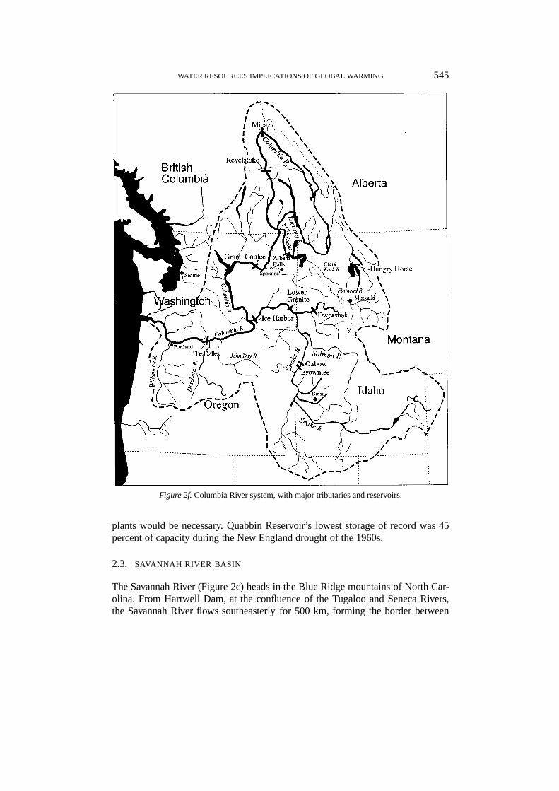
Figure 2f.Columbia River system, with major tributaries and reservoirs.

plants would be necessary. Quabbin Reservoir’s lowest storage of record was 45percent of capacity during the New England drought of the 1960s.

2.3. SAVANNAH RIVER BASIN

The Savannah River (Figure 2c) heads in the Blue Ridge mountains of North Car-olina. From Hartwell Dam, at the confluence of the Tugaloo and Seneca Rivers,the Savannah River flows southeasterly for 500 km, forming the border between


South Carolina and Georgia. Together with Hartwell Dam, the Richard B. Russelland J. Strom Thurmond reservoirs downstream form a chain of lakes 190 km long.The Savannah River drains an area of about 30,000 km2, most of which is forested.Annual rainfall ranges from 1000 to almost 2000 mm.

The most significant economic effects of the Savannah River system operationrelate to hydropower generation, recreation and flood protection. The largest pop-ulation centers in the basin are Savannah and Augusta, with 200,000 and 60,000people, respectively. The Department of Energy’s Savannah River Plant was thelargest user in the basin until 1990, when it ceased operation of three nuclearreactors. The Savannah River Plant’s demand for water was the basis for minimumreleases from Thurmond Reservoir of 102 cms, which now amply supplies lowerbasin withdrawals for municipal and industrial (M&I) and limited agricultural use.Five water use objectives are currently defined for the COE reservoirs (COE, 1989):fish and wildlife management, hydropower, recreation, water quality and watersupply.

2.4. APALACHICOLA –CHATTAHOOCHEE–FLINT RIVER (ACF) SYSTEM

The ACF basin system extends from the Blue Ridge Mountains (north of Atlanta)south to the Gulf of Mexico (Figure 2d), draining 50,800 km2, with a semi-humidclimate and mean annual runoff of about 480 mm. The ACF system comprisestwo major tributaries of roughly equal drainage area, the Chattahoochee and theFlint Rivers, which combine to form the Apalachicola River. The ApalachicolaRiver is home to a diverse range of fish species and greatly influences the nutrientinflow and productivity of Apalachicola Bay. Regulation of the main stem of theApalachicola River is minimal. The upper Flint River is also essentially unreg-ulated, while the Chattahoochee River has about 15 dams and locks operated fornavigation, flood control, water supply, recreation and hydropower generation. Thereservoir system is operated for the benefit of stakeholders in three states (Alabama,Florida and Georgia) that have different water management priorities. The largestfive projects, including Lake Sydney Lanier, are COE reservoirs.

The general operating policy for the federal dams is to release as much wateras possible for hydropower generation during the peak demand summer months,subject to the need to retain water in storage for navigation releases in the lowflow months of fall, and to meet water quality and water supply objectives duringdroughts. Reservoirs with flood control objectives have seasonally variable floodcontrol pools, and flood operation overrides other objectives when high runoffcauses encroachment on flood control storage.

2.5. MISSOURI RIVER

The Missouri River heads on the Continental Divide and flows almost 6,400 km toits confluence with the Mississippi at St. Louis (Figure 2e). The drainage area of1.37 million km2 constitutes over one-half of the drainage area of the Mississippi


River. In the downstream reaches, the climate is semi-humid and relatively tem-perate, whereas a more severe semi-arid continental climate prevails in the upperreaches. The headwater tributaries are alpine, in an area with strong orographicvariations in precipitation. The Missouri River reservoir system consists of sixCorps of Engineers reservoirs, the primary purposes of which are flood control,water supply (e.g., municipal and agricultural), navigation and power generation(recreation and fish and wildlife habitat are still incidental project uses). Thesereservoirs have aggregate active storage capacity of about 90 percent of the meanannual flow of the river at St. Louis. In addition, there are many reservoirs on themajor tributaries, notably the Platte and Kansas Rivers, which serve to regulateflow for the lower half of the basin.

2.6. COLUMBIA RIVER

The Columbia River is the fourth largest river by discharge in North Amer-ica, draining 567,000 km2 in the Pacific Northwest and 102,000 km2 in BritishColumbia, Canada (Figure 2f). The Columbia River originates at Columbia Lakeon the western slope of British Columbia’s Rocky Mountains and flows over1900 km to its mouth near Astoria, Oregon. The basin’s climate ranges frommaritime near the mouth of the main stem to arid in some of the inland valleys.The Cascade Mountains separate the coast from the interior of the basin and havea strong influence on the runoff in both areas. Occasionally, rainfall adds to therunoff, but east of the Cascades, spring snowmelt is the dominant mechanism con-trolling the shape of the seasonal hydrograph. At its mouth, the Columbia Riverhas an average annual discharge of about 7,800 cms.

More than 250 reservoirs and 100 hydroelectric projects have been built on theColumbia River and its tributaries, capturing only a third of the river’s mean an-nual flow. Approximately 75 of these projects represent the coordinated ColumbiaRiver reservoir system, which is operated by the COE and Bureau of Reclamation(BuRec) for hydropower (18,500 megawatts of firm power annually), flood control,fish migration, fish and wildlife habitat protection, water supply and water-qualitymaintenance, irrigation, navigation and recreation. In the last decade, growth in theregion and changing priorities have placed the river system under increasing stress,necessitating controversial tradeoffs between operating priorities such as fisheriesprotection and hydropower.

3. Climate Scenarios and Downscaling

The climate change scenarios used in this study are based on results from transientclimate change experiments performed with coupled ocean-atmosphere GCMs forthe 1995 IPCC assessment (Houghton et al., 1996). The approach used in the GCMtransient simulations is described in detail by Viner et al. (1994) and is summarizedby Greco et al. (1994), from which the information in this section is taken.


TABLE I

Summary of the coupled ocean-atmosphere GCMs used in IPCC transient climate changeexperiments (from Greco et al., 1994)

Model GFDL89 ECHAM1-A (MPI) UKMO

Reference Manabe et al. Cubash et al. Murphy (1995),

(1991, 1992) (1992) Murphy and

Mitchell (1995)

Atmospheric levels 9 19 11

Resolution 7.5× 4.5a 5.62× 5.62 3.75× 2.5

(degrees lat. by long.)

Integration length, yrs 100 100 75

Forcing scenario, controlb 300 ppmv 330 ppmv 323 ppmv

Climate change emission 1%/yr IPCC90 1%/yr

scenario Scenario Ac

CO2 560 ppmvd Year 57 Year 47 Year 64

Year of doubling 70 60 70

1T̄ , 2× CO2e 2.3 1.3 1.7

a Ocean model 3.75× 4.5.b Equivalent global average trace gas concentration as CO2, ppm by volume.c IPCC, 1990.d Year in which global average CO2 concentration reaches 560 ppm.e Global average temperature (◦C) in year of doubled CO2 concentration associated withsulfate aerosols and stratospheric ozone depletion (Greco et al., 1994) for a mid-rangeforecast of global economic and population growth. The actual rates of increase in atmos-pheric equivalent CO2 concentrations assumed by the models are slightly greater than theIS92a scenario, for reasons not made clear by Greco et al. (1994).

The GCM simulations were produced by three modeling centers: The Geophys-ical Fluid Dynamics Laboratory (GFDL), the United Kingdom MeteorologicalOffice (UKMO, also referred to as the Hadley Centre), and the Max PlanckInstitute (MPI). The relevant references to the coupled model runs are GFDL(model referred to internally as GFDL89): Manabe et al. (1991, 1992); UKTR:Murphy (1995), Murphy and Mitchell (1995); MPI (model referred to internallyas ECHAM1-A): Cubasch et al. (1992). Each of the models is designated by thename of the institution and the suffix TR for transient: GFTR, HCTR and MPTR. Asummary of the models and the climate change experiments is presented in Table I.

For each of the models, a base case (current climate) run was made, assumingthe atmospheric greenhouse gas concentrations (equivalent CO2) shown in Table I.Each of the models was then run with transient equivalent CO2 concentrationsstarting at the base case (control) values and increasing annually following thescenarios given in Table I. The GCMs used to produce these simulations arecoupled ocean-atmosphere models which simulate the time-dependent response of


climate to increases in atmospheric CO2. All model runs were made by the respect-ive modeling centers and were archived by the National Center for AtmosphericResearch (NCAR).

The three GCM transient runs are nominally based on emissions scenarios thatmost closely resemble the forcing used in the IPCC IS92a scenario (IPCC, 1990,1992). The IS92a scenario is an estimate of the equivalent CO2 concentration scen-ario that ‘would produce radiative forcing equal to that of all the greenhouse gases,including the negative forcing associated with sulfate aerosols and stratosphericozone depletion’ (Greco et al., 1994).

Greco et al. (1994) note several problems with the IPCC transient simulations:the use of different concentration scenarios in both the climate change runs and thecontrol runs; the existence of a ‘cold start’ problem identified by Hasselmann et al.(1992) that occurs because the models neglect the thermal lag effect associated withocean-atmosphere coupling; and inherent drift in the model simulations, which be-comes increasingly important as the length of the model simulations increases. Todeal with these problems, the IPCC transient climate scenarios are based on whatGreco et al. (1994) term the ‘simple linked method’, which couples interpretationof the GCM (three-dimensional) simulations to predictions from a simple one-dimensional climate model of Wigley and Raper (1992). As described by Grecoet al. (1994), the one-dimensional model starts with a pre-industrial climate andincorporates the effects of greenhouse gas forcing and ocean lag on a global av-erage basis to predict the rate of change of climate beginning in 1990, using theIPCC IS92a emissions scenario and a ‘warm start’ approach (that is, it accountsfor warming effects from emissions prior to 1990). Using the one-dimensionalsimulation, Greco et al. (1994) estimated global average temperature changes foryears 2020 and 2050, and used them to identify the corresponding decades (withthe same global average temperature change) for each of the GCMs. These decadeswere specified as IPCC Decades 2 and 3, respectively (Decade 1 corresponds to thecontrol run). Table II lists the model-equivalent years for each model and decade.

For the six studies reported here, the objective was to model the effect of transi-ent climate change on water resource system performance. The analysis of transientclimate change on land surface hydrology is complicated by the confounding ofnatural variability (which would occur in the absence of climate change) withthe long-term climate change signal. For this reason, forcing hydrological mod-els directly with a single GCM transient precipitation and temperature scenariocould well lead to misleading results. Ideally, assessments would be made usingensembles of GCM scenarios, each representing different statistical realizations ofthe surface hydrologic forcings corresponding to a given emissions scenario.

Given only one set of climate scenarios, and the record length limitation im-posed by the IPCC decadal analysis, such an approach was not feasible. Instead,multiple steady state analyses were performed by imposing the mean monthly(constant but seasonally varying) precipitation, temperature and solar radiationchanges for IPCC Decades 2 and 3 on the historic period of (daily) precipitation


TABLE II

GCM decades (relative to arbitrary start date)for which global average temperature changesare equivalent to years 2020 (0.53◦C) and 2050(1.16◦C) in STUGE model of Wigley and Raper(1992)

IPCC Decade 2 IPCC Decade 3

(STUGE 2020) ( STUGE 2050)

GFTR 18–27 36–45

HCTR 35–44 48–57

MPTR 24–33 49–58

and temperature records (the periods vary for the specific case studies as describedbelow, but generally are of length 40–60 years). To further resolve the GCMtransient response, three additional decades were formed by interpolating monthlyprecipitation, temperature and solar radiation changes from the GCM simulationsbetween (a) the base climate and IPCC Decade 2 (one additional case), and (b)IPCC Decades 2 and 3 (2 additional cases). For the purposes of this study, these aredesignated equilibrium climate Decades 1–5. The IPCC Decade 2 and 3 forcings,however, must be regarded as approximate. Based on ten-year averages in thewarming trajectory, they not only include error in estimation of the decadal means,but also, to some extent, incorporate the noise associated with short term (annual tosubdecadal) variability, which can obscure the long term mean change signal. Thelinear interpolation of forcings for the intermediate decades (1, 3 and 4) likewiseincorporates the same effects of shorter timescale variability in the endpoints fromwhich they are interpolated. For these reasons, the climate scenario progressionsshould be understood simply as possible future scenarios for individual decades,each set of which has been arranged into a possible progression. The correspond-ence between our decades and IPCC decades is summarized in Table III. Note thatour Decade 2 is IPCC Decade 2 and our Decade 5 is IPCC Decade 3.

In summary, rather than performing a true transient analysis, five steady-stateanalyses were performed for each GCM, where the five analyses tracked the tran-sient nature of the climate forcing. In addition to the transient GCM scenarios, wetested a doubled-CO2 scenario to provide a basis for comparison with the resultsof earlier studies (e.g., Smith and Tirpak, 1989) which generally were based ondoubled-CO2 scenarios. The GFDL doubled CO2 scenario was taken from a setof GCM results archived by NCAR for use in the Country Studies Program (U.S.Country Studies Management Team, 1994). Unfortunately, the GFDL scenario isnot directly comparable with the GFTR scenarios because our choice of doubled-CO2 GCM runs was constrained to those GCM runs that were provided to NCAR


TABLE III

Summary of steady state simulations making up the quasi-transient analysis

Equilibrium climate Correspondence to IPCC Year

decades decades correspondencea

0 IPCC ‘Decade 1’ (base case) 1990

1 Interpolation 2005

2 IPCC ‘Decade 2’ 2020



5 IPCC ‘Decade 3’ 2050

a Assuming, as per STUGE simulations, that Decade 2 is centered on year2020, and Decade 3 is centered on year 2050.

by the various GCM modeling centers. As a result, the GFDL model resolutionand other model options differed from those used in the IPCC transient scenarios.For instance, the transient scenarios used R15 resolution (about 7.5 by 4.5 degreeslongitude by latitude) whereas the R30 resolution (3.75 by 2.25 degrees) was usedin the doubled-CO2 run. Therefore, while the GFDL doubled-CO2 run can, forinstance, be interpreted in comparison with other doubled-CO2 evaluations per-formed with that set of model archives, it is difficult to interpret the results relativeto the GFDL transient run prepared for IPCC.

4. Approach

To the extent possible, the assessment approach was the same for all six casestudies. A standard experimental design, consisting of specific base case and hy-pothetical altered climate simulations and similar evaluation measures for all sites,was used to maintain consistency between the six parts of the study. Nevertheless,various intermediate steps, such as hydrologic and water resource system modelingand specific system operating objectives, differed slightly from site to site. Thestandard approach and site-specific variations are discussed in the remainder ofthis section.

A sequence of models was used to infer the water resources effects of eachof the climate change scenarios. The first step was to downscale precipitation,temperature and solar radiation changes from each of the GCM scenarios to pro-duce forcing sequences for hydrologic models of each of the river basins. Thehydrologic models generated time series of streamflow, which in turn were theforcings to water resource management models (WRMMs) of each of the reservoirsystems. Finally, the WRMMs simulated system performance for each scenario


using similar sets of performance evaluation metrics. The models used for eachcase study are summarized in Table IV.

4.1. DOWNSCALING GCM SCENARIOS

The GCM downscaling method is identical to that used in the Sacramento-SanJoaquin study (Lettenmaier and Gan, 1990) included in the EPA Reports to Con-gress (Smith and Tirpak, 1989). It simply adjusts historical observations of dailytemperature maxima and minima by adding a fixed amount to the observed values,and multiplies historical observations of daily precipitation and solar radiation by afixed amount. The adjustment factors for temperature, precipitation and solar radi-ation are the monthly average changes (from base case climate to altered climate)for the five quasi-equilibrium states sampled from the transient climate runs.

These monthly adjustments (for each steady-state ‘decade’) were interpolatedfrom the gridded GCM output fields to specified locations required for hydro-logic model inputs (i.e., grid-cell centers for the semi-distributed models of theColumbia, Missouri and ACF sites; or basin centroids for the Savannah, Boston andTacoma studies). Tables Va and Vb summarize the basin-wide average temperatureand precipitation adjustments used for each of the transient GCM scenarios.

Downscaling of the GCM simulations is necessary because GCMs’ ability toreproduce observed precipitation and temperature at the regional scale (less than107 km2) is widely recognized as poor, and there is little agreement at this scaleamong GCMs as to the magnitude and direction of changes in precipitation. Apartial discussion of this issue is given in IPCC (1996), Section 6.6.1. Detailedcomparison of precipitation and temperature fields between the GCMs and obser-vations are not available specifically for the regions we studied. For central NorthAmerica (35–50◦ N, 85–105◦W), however, the IPCC found that the best repro-duction of observed precipitation among the three models was obtained by MPTRin winter and HCTR in summer, while the worst performance was for MPTR insummer and GFTR in winter. In the worst case, a bias of minus 70 percent (MPTRin winter), many times larger than the sensitivity of the estimated MPTR doubledCO2 precipitation, was reported. For temperature in central North America, allthree models underestimated current temperatures in winter (by 5, 3 and 5◦C forGFTR, MPTR and HCTR, respectively) and two out of three overestimated temper-atures in summer (by 3 and 6◦C for GFTR and MPTR, respectively), while HCTRreproduced climatological temperatures with relatively accuracy. Better matchesbetween observed and control run (current climate) values provide higher confid-ence in future climate projections, but, in general, the reliability of GCM-derivedforcings at the regional scale must still be regarded as low. More detailed analysesof transient model run results for central North America are given in Cubasch et al.(1994), Whetton et al. (1996) and Kittel et al. (1996).

WA

TE

RR

ES

OU

RC

ES

IMP

LICA

TIO

NS

OF

GLO

BA

LW

AR

MIN

G553

TABLE IV

Water Resources Management Model Summary

Models Basins

Tacoma Boston Savannah R. ACF basin Missouri R. Columbia R.

GCMs GFTR, MPTR, HCTR, GFDL 2× CO2

Hydrologic NWSRFS snowmelt and soil moisture accounting NWS snowmelt and VIC-2L

WRMMs

Type Simulation Simulation Simulation Simulation Optimization Simulation

(STELLAr II) (STELLAr II) (FORTRAN) (STELLAr II) (HEC-PRM) (STELLAr II)

Reference Karpack and COE (1994) by Water Resources Palmer et al. (1995) COE (1991b) Hamlet et al.

Palmer (1992) Management, Inc. (1997)

Years 60 60 59 52 39 59

Timestep Weekly Weekly Weekly Monthly Monthly Monthly

Demand/operating Yes Yes Yes Yes Yes No

scenario sensitivity?

Primary uses

M&I supply X X X X

Water quality X

Instream flow X X X X X

Flood control X X X X X

Hydropower X X X X

Recreation X X X X

Navigation X X X

Irrigation X X X

Fish and wildlife X X X

‘STELLAr II’ is the name of a commercial simulation software by High Performance Systems, Inc.


4.2. HYDROLOGIC MODELS

The application of hydrologic models depended on basin size. At all sites, thetemperature-indexed National Weather Service River Forecast System (NWSRFS)snow model (Anderson, 1973) was used to estimate rain plus snow melt (whensnow is not present, the snow model simply passes the precipitation through to arainfall-runoff model). In the large basins – the Columbia, ACF and Missouri – thesnow model output became input for the semi-distributed two layer variable infilt-ration capacity model (VIC-2L) described by Nijssen et al. (1997). In the smallerBoston, Tacoma and Savannah River basins, the lumped NWSRFS Sacramentosoil moisture accounting model of Burnash et al. (1973) was used to simulatestreamflow. Tables Vc and Vd summarize the basin-wide average annual percentchanges in PET and streamflow for each of the transient GCM scenarios.

The use of different hydrologic models for different study sites is not likelyto have much effect on the results, insofar as a calibration process (to currentclimate) was undertaken for each site. The most problematic aspect of the useof precipitation-runoff models for climate change assessment is the implicit as-sumption that parameter estimates obtained from historical data are applicable toalternative climates. As long as the differences between current and altered climateare modest compared to the observed interannual and interseasonal variability inthe historical records of the atmospheric forcings, which is usually the case, thisshould not be a serious issue. Furthermore, for assessments that use the pertur-bation method of climate scenario development, changes are interpreted relativeto a base case hydrological simulation using historical observed data. Because thealtered climate scenarios are variations of the same input used in the base casehydrological model simulations, and hence should induce a positive correlation inthe base case and altered climate simulation errors, differencing should result inerrors in predicted effects that are smaller than the model verification error.

Regardless of which hydrologic model was used, calibration was first per-formed by examining observed time series of precipitation and temperature (forat least a ten-year period) and comparing observed and simulated streamflow.Model parameters were adjusted within physically plausible ranges so that thedaily streamflow peaks, baseflow recession, monthly flow volumes and long termaverage flow volumes matched as closely as possible. The primary calibrationparameters for the NWSRFS model were the moisture storage zones (5) and therecession constants (k1 andk2), and for the VIC-2L model were the moisture stor-age zones (2) and the infiltration parameters. Greater detail about model calibrationis given in Lettenmaier et al. (1998a–f).

4.3. WATER RESOURCE MANAGEMENT MODELS(WRMMS)

The WRMMs take output from the hydrologic models (streamflow) and, in somecases, physical climate variables such as precipitation and temperature, which areused in the demand estimates. Given sequences of streamflow, the models predict


the performance of the systems in terms of variables such as flows and storages,hydropower production, and the ability of the system to meet demands for wa-ter and to meet constraints such as minimum instream flows. The six WRMMswere adapted from existing models for each site. The WRMMs use longer timesteps than the hydrologic models – either weekly (e.g., for Tacoma and Boston) ormonthly.

The WRMMs used for the Tacoma, Boston, ACF and Columbia systems weredetailed simulation models that track water through the reservoir system and in-clude the effects of reservoir regulation through representation of the rule curvesthat are, at least nominally, used in practice. In each of these cases, the processof model development involved participation and review by water users, who in-sisted on demonstration of model validity. This was generally accomplished viareplication of observed storage and flow levels given observed inflows, evaporation,withdrawals and other system parameters. The WRMM used in the Savannah Riverstudy was a FORTRAN-based simulation model which incorporated a routine thatoptimized power production given prescribed end-of-period releases. The model(developed by the South Carolina Division of Water Resources) incorporatedcurrent power production targets, reservoir rule curves and environmental flowconstraints. The Missouri River system was modeled in HEC-PRM, a U.S. ArmyCorps of Engineers optimization package that maximizes reservoir system per-formance relative to operating objectives (such as power production) given a setof system constraints (e.g., economic penalty functions for flood control, powerreleases or agricultural withdrawals). The model and modeling framework (HEC-PRM) are described in COE (1991a, b). Based on validation runs, the optimizationmodel reproduced observed storages and discharges somewhat less faithfully thandid the simulation models.

4.4. SYSTEM PERFORMANCE METRICS

A standard approach for evaluating system performance under the climate scen-arios was taken for all of the case studies. The intent of the studies was to provideresults in terms that might be useful to system managers and decision-makers. Twotypes of system performance metrics were used: threshold-type metrics and abso-lute metrics. Absolute metrics are simple measurements of system states or outputs,such as reservoir elevations, flow levels, electricity generation (e.g., in MWh) or itseconomic value. Threshold metrics are defined relative to a performance target,such as a minimum instream flow level, and measure success or failure relative tothe target. The threshold metrics were three indices proposed by Hashimoto et al.(1982) – reliability, resiliency and vulnerability. Reliability is defined as the per-centage of time that the system operates without failure (the number of successfulperiods divided by the total number of simulation periods). Resiliency is a unitlesscoefficient relating to the ability of the system to recover from a failure, definedas the probability that a shortfall event lasts only a single period. Vulnerability


TABLE Va

Average annual temperature changes for the transient and 2× CO2 simulations

Average annual temperature change (◦C) for GFTR, HCTR, MPTR respectively

Case study Decade 1 Decade 2 Decade 3 Decade 4 Decade 5 2× CO2

Tacoma 0.8, 0.4, 0.3 1.6, 0.8, 0.5 2.2, 1.4, 0.9 2.7, 1.9, 1.4 3.3, 2.5, 1.8 3.5

Boston 1.8, 1.9, 1.2 1.8, 3.8, 3.4 2.5, 4.2, 2.6 3.3, 4.7, 2.8 4.0, 5.1, 3.0 5.9

Savannah 1.1, 1.3, 0.8 2.1, 2.5, 1.5 2.5, 2.7, 1.7 3.0, 2.9, 1.8 3.4, 3.1, 2.0 5.9

ACF 0.9, 1.1, 1.0 1.8, 2.1, 2.0 2.2, 2.4, 2.1 2.7, 2.6, 2.3 3.1, 2.9, 2.4 3.8

Missouri 1.0, 1.5, 1.1 1.9, 3.0, 2.2 2.5, 3.1, 2.5 3.0, 3.3, 2.9 3.6, 3.4, 3.2 4.4

Columbia 0.9, 0.8, 0.6 1.8, 1.5, 1.2 2.3, 2.0, 1.7 2.9, 2.5, 2.1 3.4, 3.0, 2.6 3.9

is defined as the average severity (magnitude) of failures. Several absolute metricsand the three threshold metrics were calculated to characterize system performancefor each system operating objective, so as to give a multi-faceted, comprehensivemeasurement of the system’s performance for each objective. Because the multiplemetrics used for each site are too numerous to present here, a single representativemetric for each operating objective, for each system, is displayed in the resultssummaries of Figures 3–8.

4.5. DEMAND GROWTH AND ALTERNATIVE OPERATIONAL SCENARIOS

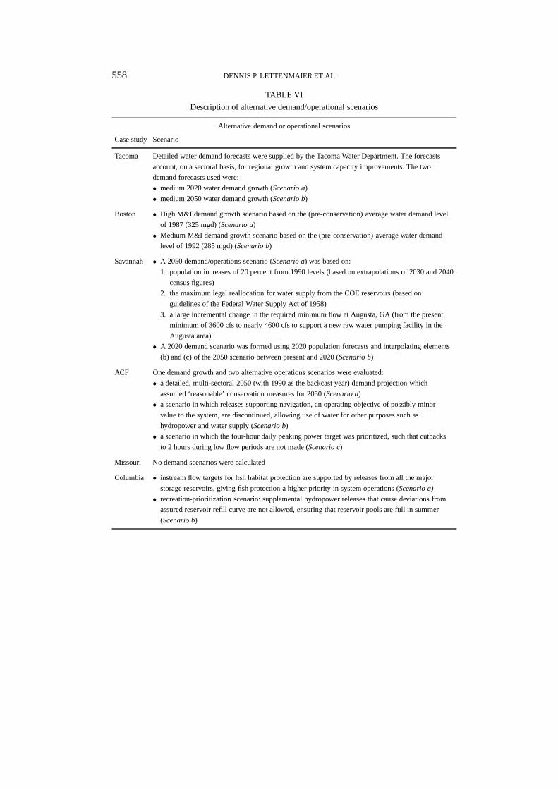
Where possible, the effects of climate change were compared with the effects ofnon-climate related changes that could plausibly take place over the same periodas the climate changes measured in these assessments (1990–2050). These non-climate changes might arise due to predicted demand changes (for instance, dueto population growth) or shifts in other factors affecting system operation. Forexample, the current debate over the importance of hydropower relative to fisheriesprotection on the Columbia River could lead to a prioritization of instream flowaugmentation releases over releases for hydropower, a significant change on whichone of the alternative operational scenarios for that system was based. Similarly,for the Savannah River and ACF basin study sites, alternative operational scenarioswere created to examine such changes as discontinuation of navigation support, in-creased instream flow requirements and increased hydropower demand. For largelymunicipal supply systems, such as Boston and Tacoma, the effects of demandgrowth were examined in detail. Table VI describes the demand growth/operationalscenarios by site.


TABLE Vb

Average annual precipitation changes for the transient and 2× CO2 simulations

Average annual precipitation change (%) for GFTR, HCTR, MPTR, respectively


Tacoma 6, 2, –1 11, 3, –2 10, 3, –2 8, 2, –2 7, 2, –2 24

Boston 3, 6, –2 5, 12, –4 7, 11, –5 9, 10, –5 10, 9, –6 15

Savannah 2, 4, 2 5, 8, 3 9, 9, 3 13, 9, 3 16, 9, 3 13

ACF 2, 5, 2 3, 9, 4 7, 7, 3 11, 5, 3 14, 4, 3 –4

Missouri 3, –5, –11 6, –10, –22 7, –5, –22 8, –1, –23 8, 3, –23 9

Columbia 6, –1, –5 11, –2, –11 9, –1, –10 7, –1, –9 5, 0, –9 25

TABLE Vc

Average annual PET changes for the transient and 2× CO2 simulations

Average annual PET changes (%) for GFTR, HCTR and MPTR, respectively


Tacoma 4, 0, 0 10, 0, 1 14, 4, 4 17, 8, 8 18, 14, 12 20

Boston 1, 6, 6 4, 10, 10 7, 12, 13 9, 13, 13 10, 13, 13 19

Savannah 1, 3, 2 7, 9, 3 10, 10, 4 11, 11, 6 11, 11, 6 18

ACF 4, 4, 3 7, 7, 7 10, 9, 8 12, 11, 9 14, 12, 10 18

Missouri 7, 11, 7 14, 23, 16 18, 24, 18 22, 25, 21 19, 24, 19 32

Columbia 6, 5, 4 12, 11, 8 16, 14, 11 21, 18, 15 27, 21, 18 28

TABLE Vd

Average annual system inflow changes for the transient and 2× CO2 simulations

Average runoff changes (%) for GFTR, HCTR and MPTR, respectively


Tacoma 10, 7, 2 19, 11, 4 17, 10, 4 16, 10, 4 15, 9, 4 33

Boston 4, 9, –3 7, 19, –3 9, 16, –3 12, 14, –3 15, 13, –1 17

Savannah 5, 3, –3 7, 5, –4 11, 3, –4 17, 3, –5 23, 3, –4 7

ACF 4, 2, –5 11, 8, –5 15, 3, –7 20, –1, –7 25, –3, –6 –21

Missouri 3, –26, –20 6, –34, –36 1, –31, –35 –3, –27, –35 –6, –24, –34 2

Columbia 6, –2, 8 11, –3, –15 6, –4, –16 2, –6, –16 –1, –6, –16 23


TABLE VI

Description of alternative demand/operational scenarios

Alternative demand or operational scenarios

Case study Scenario

Tacoma Detailed water demand forecasts were supplied by the Tacoma Water Department. The forecasts

account, on a sectoral basis, for regional growth and system capacity improvements. The two

demand forecasts used were:

• medium 2020 water demand growth (Scenario a)

• medium 2050 water demand growth (Scenario b)

Boston • High M&I demand growth scenario based on the (pre-conservation) average water demand level

of 1987 (325 mgd) (Scenario a)

• Medium M&I demand growth scenario based on the (pre-conservation) average water demand

level of 1992 (285 mgd) (Scenario b)

Savannah • A 2050 demand/operations scenario (Scenario a) was based on:

1. population increases of 20 percent from 1990 levels (based on extrapolations of 2030 and 2040

census figures)

2. the maximum legal reallocation for water supply from the COE reservoirs (based on

guidelines of the Federal Water Supply Act of 1958)

3. a large incremental change in the required minimum flow at Augusta, GA (from the present

minimum of 3600 cfs to nearly 4600 cfs to support a new raw water pumping facility in the

Augusta area)

• A 2020 demand scenario was formed using 2020 population forecasts and interpolating elements

(b) and (c) of the 2050 scenario between present and 2020 (Scenario b)

ACF One demand growth and two alternative operations scenarios were evaluated:

• a detailed, multi-sectoral 2050 (with 1990 as the backcast year) demand projection which

assumed ‘reasonable’ conservation measures for 2050 (Scenario a)

• a scenario in which releases supporting navigation, an operating objective of possibly minor

value to the system, are discontinued, allowing use of water for other purposes such as

hydropower and water supply (Scenario b)

• a scenario in which the four-hour daily peaking power target was prioritized, such that cutbacks

to 2 hours during low flow periods are not made (Scenario c)

Missouri No demand scenarios were calculated

Columbia • instream flow targets for fish habitat protection are supported by releases from all the major

storage reservoirs, giving fish protection a higher priority in system operations (Scenario a)

• recreation-prioritization scenario: supplemental hydropower releases that cause deviations from

assured reservoir refill curve are not allowed, ensuring that reservoir pools are full in summer

(Scenario b)


5. Results

Tables Va–d showed average annual changes in temperature, precipitation, po-tential evapotranspiration (PET) and streamflow (system inflow), respectively,associated with each decade and GCM, for the six case studies. Figures 3 through8 summarize the results of these changes for system performance, categorized bysystem operating objective. A table entry or figure annotation of ‘NC’ indicates thatthe statistic was not calculated for a particular case study. In one case (flooding onthe Savannah River), results were interpolated to estimate results for decades forwhich the metric had not been calculated.

5.1. CLIMATIC CHANGES

Table Va shows that the temperature changes from each case study and for eachGCM differ appreciably from the global average warming predicted for Decades2 and 5 (0.53◦C and 1.16◦C, respectively). Notably, for the Savannah River, ACFbasin and Missouri River case studies, most of the Decade 5 increase in warmingwould occur by Decade 2, in contrast to the steadier trend of the global average.Temperatures would increase between each decade (from the base case throughDecade 5) and in all but one instance, the increases would be larger than thepredicted global averages. The range of temperature increases in Decade 2 werefrom 0.5◦C for MPTR, for Tacoma, to 3.8◦C for HCTR for Boston. The 2× CO2

scenario, in every case, showed larger temperature increases than any of the tran-sient climate scenarios; the largest increase, 5.9◦C, occurred for the Boston andSavannah River sites.

The precipitation changes, shown in Table Vb, were less consistent from siteto site than the temperature changes. At most sites, the GFTR scenarios producedthe largest increases in precipitation, especially by Decade 5. For Tacoma and theColumbia River, the increases leveled off or grew smaller after Decade 2, whereasfor the other sites the increases progressed by decade. The MPTR scenarios, inall sites except for the ACF basin and Columbia River, had the smallest increasesor largest decreases in each decade. In every case, these changes leveled off orreversed direction after Decade 2. Changes for the HCTR scenarios behaved simi-larly. In magnitude, HCTR precipitation changes tended to fall between the GFTRand MPTR changes for the Tacoma, Columbia and Missouri River sites, but couldbe larger than the GFTR or smaller than the MPTR scenario precipitation in indi-vidual scenarios for the other sites. Precipitation changes for the 2×CO2 scenariosfor the Tacoma and Boston systems were larger than for the transient scenarios,whereas for the Savannah and Missouri River sites, the 2× CO2 scenario changewas about equal to the GFTR scenario changes in later decades. In the ACF basin,the 2× CO2 scenario produced precipitation decreases, in contrast to all of theACF basin transient scenarios. The Columbia River 2× CO2 scenario’s large (25percent) increase in precipitation also contrasted with the transient scenarios.


5.2. HYDROLOGIC CHANGES

Table Vc shows changes in PET. Mostly driven by temperature changes, PETchanges were positive for every scenario at every site. The largest average annualincreases for the transient scenarios were 27 and 24 percent for the Columbia(GFTR) and Missouri (HCTR) River basins, respectively, in Decade 5. The smal-lest Decade 5 increase was 6 percent, for Savannah (MPTR). The 2×CO2 scenarioshad slightly higher PET than the highest Decade 5 scenario for every site.

In general, changes in PET were consistent with temperature changes in dir-ection, timing (i.e., relative interdecadal changes, such as the majority of thewarming for HCTR occurring by Decade 2) and magnitude. Precipitation changesalso appeared to moderate PET changes, however. Exceptions to the generalrelationship between temperature and PET also resulted from variations in theseasonal distribution of temperature changes among the climate change scenarios(increased temperatures in the summer months contribute disproportionately toannual changes in PET); hence comparison of annual temperature changes withannual PET could be misleading. For example, although the temperature changesfor the MPTR scenarios in the Boston study were little over half those of the HCTRscenarios, the PET increases for the two sets of scenarios were very similar.

Table Vd shows changes in system inflows (streamflow) for each case study.For most of the case studies, there is little agreement between the GCM scenariosin terms of magnitude or direction. In some series of scenarios – e.g., the SavannahRiver (GFTR) – increases or decreases progressed monotonically from Decade 1through Decade 5. In other cases – the Missouri River (all GCMs), for Tacoma(GFTR and HCTR), Boston (HCTR), the Savannah River (HCTR), the ACF basin(HCTR) and the Columbia River (GFTR) – changes in streamflow in Decade 2were reversed in Decades 3, 4 and 5. These reversals generally can be traced toopposing hydrologic effects of increased temperature (which tends to result instreamflow decreases) and increased precipitation (leads to increased streamflow).For several sites, such as Tacoma, for at least one GCM series, the largest runoffchanges occurred between the base case and Decade 2, with little to no furtherchange between Decade 2 and Decade 5. Annual average changes ranged froma 25 percent increase in the ACF basin (GFTR) to a 34 percent decrease for theMissouri River (MPTR) in Decade 5.

5.3. SYSTEM PERFORMANCE EFFECTS

Figures 3 through 8 show system performance results categorized by objective(hydropower, M&I and agricultural supply, flooding, recreation, instream flowaugmentation and navigation, respectively) for all sites, using the metrics listedin the figures. Although a suite of metrics was used in each of the studies tocharacterize each system’s performance with respect to each major operating ob-jective, we focus here on a single metric for each site and objective that appearedto represent adequately the system’s sensitivity to the climate change scenarios.


Where possible, percent changes in absolute measures of system state or output(such as energy generation or recreation-related income) are shown in Figures 3–8. Otherwise, the net changes in the system’s reliability in satisfying a prescribedthreshold of performance (such as meeting contractual monthly energy targets)are shown. Note that not all operating objectives are relevant in each case study.Also shown in Figures 3–8 are the results of the ‘demand/operational scenarios’discussed in Section 4.5 (and detailed in Table VI).

Figure 3 shows that power operations would be most sensitive to climate changefor the Missouri River, where both the HCTR and MPTR scenarios would result indeclines (in reliability of meeting monthly energy targets) of between 15 and 35%.Small increases in reliability were found for GFTR in Decades 1 through 3 and forthe 2× CO2 scenario. For the Columbia River, reliability of firm energy showedprogressive declines in the transient scenarios, while the 2× CO2 scenario hadonly a negligible decrease. Changes for the two alternative operational scenarioswere on the order of those for the most severe climate scenarios. For the SavannahRiver, two out of the three GCMs led to increases in power production of between3 and 25 percent, while the MPTR scenarios had slight declines. The 2× CO2

scenario led to increases in the range of the GFTR Decade 2 and 3 scenarios, whiledemand growth effects lie at the lower end, in magnitude, of the range of all of theclimate change effects. For the ACF basin, the effects for GFTR and MPTR weregenerally in the same direction as those for the Savannah River, but smaller. Thelargest changes (declines) were for the HCTR scenarios and the 2×CO2 scenario.The system’s sensitivity to demand/operational changes was comparable to thesensitivity to climate change effects. It should be noted that the Columbia Riversystem has by far the largest installed hydropower generating capacity (18,500MW) of the systems studied; by comparison, the installed generating capacity ofthe Missouri River system, the Savannah River system, the ACF basin are 6,770,1,990 and 560 MW, respectively.

Figure 4 shows that M&I supply would be fairly robust to climate change forthe smaller systems, while moderate declines in performance would occur for theMissouri and Columbia River systems. It should be noted, however, that for theMissouri River, M&I supply accounts for a relatively minor portion of systemwater allocation, whereas for the smaller Boston and Tacoma systems, M&I supplyis a first priority use (the Tacoma system also prioritizes flood control). Despitetheir relative insensitivity to climate changes, the Boston and Tacoma systems arehighly sensitive to demand growth: 3 and 39 percent declines in reliability wouldresult from returns to (the higher than present) 1992 and 1987 levels of demandfor Boston; and for Tacoma, 3 and 20 percent declines in reliability would resultfrom demands levels current forecasted for 2020 and 2050. For the Columbia Riversystem, where M&I use is trivial, agricultural withdrawals (measured by SnakeRiver irrigation) showed minor to moderate (∼15 percent) responses to climatechange, while the operational scenarios system had no effect on withdrawals. In

562D

EN

NIS

P.L

ET

TE

NM

AIE

RE

TA

L.

Figure 3. Climate and demand change effects on hydropower for each system as measured by either percentage changes in an absolute measure or netchanges in a hydropower-related reliability metric (see Table VI for description of demand scenarios).

WA

TE

RR

ES

OU

RC

ES

IMP

LICA

TIO

NS

OF

GLO

BA

LW

AR

MIN

G563Figure 4. Climate and demand change effects on M&I or agricultural supply for each system as measured by either percentage changes in an absolute

measure or net changes in a M&I supply-related reliability metric (see Table VI for description of demand scenarios).


the Savannah River and ACF basin systems (not shown), M&I supply performancewas insensitive to the climate and demand/operational changes evaluated here.

As shown in Figure 5, climate change would cause flood risk to increase for sev-eral of the climate change scenarios, at all of the sites except for the Columbia Riverbasin. For Tacoma and the Savannah River, flooding effects increased substantiallyand progressively for all scenarios. For the ACF basin, substantial changes in floodrisk occurred for the transient scenarios, but the changes varied in direction forthe different climate scenarios. For the Columbia River system, flood risk changedmost (decreased) for the 2×CO2 scenario. For the Missouri River, flooding effectsincreased for all scenarios, but to a smaller degree than at other sites. For theTacoma and ACF River systems, the 2× CO2 scenario also led to changes muchlarger than for the transient scenarios, in various directions. In comparison to theclimate scenarios, the demand growth/operational changes had little or no effect onflooding. Note that due to the long timesteps (week or month) of the WRMMs, theestimation of flood related effects is at best approximate; hence, the metrics shownhere are more qualitative than quantitative.

Figure 6 summarizes the results for recreation-related effects. For the Savannahsite, climate change effects led to increases in recreation-related regional income,but were smaller than the effects of population (based on year 2020 and 2050 popu-lation projections). For the ACF basin, results were conflicting for both the climatechange scenarios and the alternative operational scenarios, but indicate that theclimate change effects, while significant, would be smaller. The 2× CO2 scenariofor the ACF basin was significantly worse than the transient scenarios. For the Mis-souri River system, climate change had little effect on recreational uses, while theColumbia River experienced considerable (10–50 percent) declines in recreation-level reservoir elevation reliability for all of the transient scenarios, worsening overtime. The fishery preservation operational scenario affected recreation to about thesame degree as climate change, while the recreational alternative improved it onlyslightly.

Figure 7 shows the sensitivity of instream flow requirements for the Tacoma, Sa-vannah River and Columbia River systems. For all three systems, effects of climatechange would be on the order of the effects of demand/operational changes: thelargest change in instream flow reliability due to climate change was just over 10%(a decline) from the base case. For all three systems, the largest declines occurredfor the MPTR scenarios and the only increases occurred for the GFTR scenarios.The 2× CO2 scenarios led to smaller effects in each case than the later decadesof the transient scenarios. For both the Tacoma and Savannah River systems, de-mand/operations changes would be on the order of the results for the Decade 5scenarios. For the Columbia River system, however, the fishery protection scenariosignificantly improved the reliability of instream flow, while the recreation poolprotection scenario had little effect.

As shown in Figure 8, the influence of climate change on navigation for threecase studies varies. For the ACF basin, the transient scenarios caused slight changes

WA

TE

RR

ES

OU

RC

ES

IMP

LICA

TIO

NS

OF

GLO

BA

LW

AR

MIN

G565Figure 5.Climate and demand change effects on flooding for each system as measured by either percentage changes in an absolute measure or net changes

in a flooding-related reliability metric (see Table VI for description of demand scenarios). Decades 1, 3 and 4 for the Savannah River basin are interpolated.

566D

EN

NIS

P.L

ET

TE

NM

AIE

RE

TA

L.

Figure 6.Climate and demand change effects on recreation for each system as measured by either percentage changes in an absolute measure or net changesin a recreation-related reliability metric (see Table VI for description of demand scenarios).

WA

TE

RR

ES

OU

RC

ES

IMP

LICA

TIO

NS

OF

GLO

BA

LW

AR

MIN

G567Figure 7.Climate and demand change effects on instream flows for each system as measured by either percentage changes in an absolute measure or net

changes in a instream flow-related reliability metric (see Table VI for description of demand scenarios).

568D

EN

NIS

P.L

ET

TE

NM

AIE

RE

TA

L.

Figure 8.Climate and demand change effects on navigation for each system as measured by percentage changes in absolute performance measures or netchanges in navigation-related reliability metrics (see Table VI for description of demand scenarios).


in the reliabilities of maintaining sufficient channel depths, while the 2× CO2

scenario and one operational change scenario (cessation of navigation support)caused larger declines in reliability. Navigation in the Columbia River system isrepresented by the reliability of lock operations on the Snake River. The 2× CO2

scenario showed a large decrease in this reliability, while for the transient scenarios,changes in reliability were smaller, peaked in Decade 2, and varied in directionbetween the GCM series. For the Missouri River, where the base case reliability ofmeeting system-wide navigation targets was only 10 percent, the GFTR Decade 1scenario increased by 1 percent before decreasing almost to zero, which was thereliability for all of the MPTR and HCTR scenarios. The 2×CO2 scenario showeda smaller decrease of 5 percent.

6. Interpretation

6.1. TACOMA SYSTEM

Streamflow changes (Table Vd), in contrast to PET changes, were consistent withchanges in precipitation, although these were influenced secondarily by changesin PET and temperature. Temperature changes were important because the hy-drograph of the major component of system inflows (which are derived from theCascade Mountain headwaters) exhibits a strong spring snowmelt signal that is pro-gressively shifted earlier in the year, toward winter, by the increasing temperaturesof the scenarios. In progressive decades, a smaller portion of the annual precipita-tion falls as snow, causing slightly increased runoff magnitudes that compound theoverall changes in annual precipitation volume.

These two effects of climate change on runoff – changes in magnitude andseasonality – were the primary factors affecting system performance. Increases inflooding (Figure 5) reflected an increase in both the average magnitude of runoffand in the variability of the runoff scenario. M&I supply reliability (Figure 4),which is 100 percent for the base case, was unaffected by increases in runoff,despite increases in base water demand as a results of temperature increases. Inall cases, M&I supply was protected by legal priority from even large declines insystem inflows. Instream flow requirements (Figure 7), however, were met less fre-quently despite the overall runoff increases due to the shift in seasonality of runoff(unfortunately, this dynamic cannot be seen from the annual summary of statisticspresented in Section 5; greater detail is given in Lettenmaier et al. (1998a)). HAHreservoir refills in the spring, too late to capture winter runoff; thus for the laterdecades, HAH does not always refill and has difficulty augmenting flows duringthe drawdown period in autumn, when instream flow requirements are highest.

The demand growth scenarios were based on medium M&I use forecasts for2020 and 2050. In contrast to climate change effects, this growth in demand greatlydegraded the reliability in M&I performance and caused a comparable decline in


the reliability of meeting instream flow requirements (because the priority M&Idemand leaves less water in the Green River). The effects of demand changes onflood control operations were not measured.

6.2. BOSTON SYSTEM

As with the Tacoma system, changes in runoff for the Boston system (Table Vd)were influenced mainly by precipitation changes and changes in PET. GFTR runoffincreased progressively, MPTR runoff diminished as precipitation declines wereexacerbated by PET increases, and the initial HCTR increases in runoff were inthe later decades slightly eroded by weaker precipitation increases relative to PETincreases. Although the Boston system inflow hydrograph has a snowmelt compon-ent, it is less significant than for Tacoma. For this reason, the sensitivity of runoffto temperature changes for the Boston site acted primarily through changes in PET.

For the Boston system, runoff changes coupled with climate-driven changesin demand, estimated via the IWR-Main model (PMCL, 1994), were the primaryfactors affecting system performance. M&I supply reliability (Figure 4), which is100 percent for the base case, was obviously unaffected by the increases in runoffassociated with the GFTR, HCTR and 2× CO2 scenarios. For the MPTR scen-arios, however, decreasing runoff compounded by increasing demand (due mainlyto increasing temperature) led to slight declines in water supply reliability. The vul-nerability of the system to demand increases is underscored by severe degradationof supply reliability in response to the demand growth scenarios (base demandsequivalent to 1987 and 1990 levels). Because the Boston system is used primarilyfor water supply, climate change and demand growth effects on other aspects ofsystem performance were not measured.

6.3. SAVANNAH RIVER SYSTEM

Changes in runoff (Table Vd) for the Savannah River basin reflected mainly pre-cipitation changes, and to a lesser extent, changes in PET. For example, runoff inthe HCTR scenarios increases through Decade 2 but decreases thereafter, perhapsas a result of the interaction between the initial increase (in Decades 1–3) andleveling off (Decades 4–5) in precipitation, and the continuing increase in PET.Likewise, the small decreases in runoff for the MPTR scenarios probably derivedfrom combination of modest increases in precipitation and greater increases in PET.

For the Savannah system, the primary factor affecting system performancein most categories was runoff changes – both magnitude and variability. For allscenarios, runoff variability increased progressively and significantly as comparedto the base case. Hence, while not all scenarios had mean runoff increases, allscenarios did have progressively increasing flood damages (Figure 5). Changesin power production (Figure 3) were consistent with system inflow changes, aswere effects on instream flow reliability (Figure 7), although the priority of powerproduction among operating objectives prevented gains in instream flow reliability


that might otherwise have been possible given the increased runoff of the GFTRand HCTR scenarios. Due to the large amount of storage in the basin relative towithdrawal or non-power release demands, M&I supply reliability (Figure 4) wasinsensitive to the changes in runoff associated with the climate scenarios. Reser-voir pools were barely affected by the modest changes in runoff of the climatechange scenarios. Finally, recreation performance (Figure 6), measured in terms ofrecreation-related regional income, increased for all of the scenarios in proportionto increases in temperature, which spurred recreation demand (visitation).

The two demand growth scenarios, based on projected increases in population,withdrawals and system release requirements, had the general effects of remov-ing water from the system while also constraining its releases. Hence, powerproduction declined and instream flow releases were curtailed, both to an ex-tent comparable to the MPTR climate change effects. Recreation performanceincreased as a result of increased population growth in the region. Flooding wasmostly unaffected because, on average, reservoir pools did not drop much dueto the greater withdrawals and the variability of inflows was unchanged by thedemand scenarios. In contrast to the Tacoma and Boston systems, the demandscenarios for the Savannah River system generally led to effects that were smalleror comparable in size to the climate change effects.

6.4. ACF BASIN SYSTEM

The relatively large increases in runoff in the GFTR scenarios and in the earlyHCTR decades can be attributed to precipitation increases. For the MPTR andHCTR scenarios, declining runoff in later decades resulted from faltering increasesin precipitation coupled with continuing increases in PET. In the 2×CO2 scenario,the notably large decrease in runoff resulted from a minor decrease in precipitationcombined with a large increase in PET.

There is relatively little consistency among climate scenarios as to the im-plications of climate change for the ACF system. System performance changescan largely be explained by the average changes in inflow, relative to the basecase, that characterize each climate scenario. Effects on navigation (Figure 8) andflooding (Figure 5) metrics are related to average changes in inflows for theentirebasin because measurement of effects on these objectives occurs downstream of allsystem inflow points. In contrast, effects on recreation (Figure 6), which dependson full reservoirs, on power generation (Figure 3), which is proportional to flowand reservoir elevation, and on water supply (Figure 4) are determined by aver-age changes inupperbasin inflows, which constitute most of the system storageinputs. Upper basin inflow changes differ somewhat from changes in total systeminflow. For the ACF River basin, different GCMs lead to various estimations ofhydrology (Table Vd) under climate change, and the water resources managementimplications for the GCMs vary accordingly.


M&I supply, unlike other system objectives, was insensitive to differences in theclimate scenarios. Under current operations, M&I supply has by default the highestpriority of all system objectives, so unlike other objectives, water supply is notexplicitly curtailed if reservoirs are drawn down. Thus water supply (as modeledhere) is relatively invulnerable to hydrologic changes that would be wrought byglobal warming (as interpreted from the GCM scenarios).

Given the same flow regime in the base case and the operational alternativescenarios, system performance under the alternative operational scenarios wasdetermined mostly by changes in system storage that resulted from alternativeoperations. The peak power operational scenario reduced reservoir storage relativeto the base case, thereby limiting recreation and navigation (due to the greaterconstraint placed on the timing of releases), but few of the other objectives. Inthe ‘no-navigation support’ scenario, the system was freed from the constraint offlushing water downstream to maintain a full channel depth at Blountstown, AL,allowing system storage to remain high relative to the base case. Accordingly,the storage-dependent recreation measures improved significantly, as did powermetrics, while navigation, no longer a driver of system operations, suffered. TheM&I demand growth scenario simply extracted more water from the system, aneffect that was concentrated at the upstream end of the basin. The change in flowgoing through the system, however, was still smaller than the changes associatedwith many of the alternate climate scenarios. System storage was marginally lowrelative to the base case, causing power metrics to decline slightly and recreationperformance measures to decrease as well. Navigation reliability also declined, butminor flood reduction resulted from greater consumptive use in the upper end ofthe basin.

With regard to system objectives other than flood control, the GFDL 2× CO2

scenario produced the worst system performance of the alternate climate scenarios,particularly compared to the GFTR scenarios, as a result of substantial decreasesin inflows.

6.5. MISSOURI RIVER SYSTEM

Annual runoff changes, the largest for any study site, again reflected the mod-eration of changes in precipitation by changes in PET. Snow accumulation andablation, which would be affected directly by temperature increases, are importanton the western margin of the basin but make only a modest contribution to totalrunoff. For the MPTR and HCTR scenarios, declining precipitation coupled withincreasing PET led to substantial decreases in runoff, making the Missouri Riversite the most sensitive to global warming of all the study sites from a hydrologicstandpoint. The small increases in precipitation (Table Vb) for the GFTR scenariosled to small increases in runoff in the initial decades, but these gains were erasedin later decades by rising PET. For the GFDL 2× CO2 scenario, the precipitationincrease led to a slight increase in runoff despite a significant increase in PET.


As in the Savannah River and ACF basin sites, changes in system performanceprimarily reflected changes in streamflow. In general, the large flow reductionsfor the HCTR and MPTR scenarios favored flood control, but were detrimentalto all other system objectives. Hence, for water supply, navigation, hydropowerand river-based recreation, the altered climate scenarios resulted in modest to ma-jor impairments for the HCTR and MPTR scenarios, but small improvements inhydropower and navigation for the earlier GFTR scenarios.

6.6. COLUMBIA RIVER SYSTEM

While the results at most sites demonstrate that PET would increase significantlyas a result of climate change, causing reduced runoff, the 2× CO2 scenario forthe Columbia River site shows that concurrent, significant precipitation increasesmay be able to more than offset the effects of increased PET and support increasesin runoff. From a water supply perspective, then, site specific assessments mustconsider precipitation changes to be at least as important as temperature changesin determining runoff.

For the Columbia River system, changes in system performance for energy,flood control and fishery protection can be explained mainly as a result of meanstreamflow changes for the various scenarios. The large decrease in streamflow thatoccurred under the HCTR and particularly the MPTR scenarios degraded energyperformance (Figure 3), instream flow reliability (Figure 7) and irrigation with-drawal reliability (Figure 4). The increased streamflow for the GFTR and 2×CO2

scenarios resulted in nearly opposite effects for these objectives. Navigation, meas-ured via flows on the Snake River, was more limited by high flows than low flows –hence, the flow increases for the 2×CO2 scenario translated into a large decline inreliability. Changes for the transient scenarios were modest in comparison, peakedin Decade 2, and varied in direction between GCM series. The reliability of fullrecreation pools was eroded by streamflow decreases in the transient scenarios,particularly the MPTR scenarios, but it was difficult to see why, for example, theeffects for the GFTR and HCTR scenarios were so similar, given the differencesbetween them in terms of streamflow. The lack of a consistent relationship betweenstreamflow changes and system performance changes on the annual scale indicatesthat subtleties of timing of runoff and volume of seasonal runoff for individual runswere also important determinants of performance. For example, the seasonal tim-ing of runoff associated with the warmer climate scenarios benefited hydropowerproduction, for which demand is highest in the winter, because earlier timing ofsnowmelt was compensated by increased winter runoff.

In general, the performance of the Columbia River system would be fairly ro-bust to the effects of climate change. For most objectives, performance dependedon the ability of the system to maintain full reservoirs and support minimum re-leases, and was affected at most to the degree of the largest streamflow reductions(around 15 percent for the MPTR scenarios).


7. Summary and Conclusions

Although this paper is directed primarily toward inferring the possible effects ofclimate change on the performance of water resource systems, an integral part ofeach of the studies was downscaling of climate scenarios and modeling their effectson the hydrology of the six systems. While the six sites differ in their climatology,hydrology, system configurations and operating purposes, there are nonethelesssome commonalties in the climate scenarios and responses. We attempt to identifythese below.

7.1. CLIMATE CHANGE

Temperature changes (increases) for the transient scenarios tended to be smallerthan the temperature increase for the 2×CO2 scenario used in this and many earlierstudies. The transient scenario temperature increases grew progressively from Dec-ade 1 through Decade 5 for all basins, although for several studies, particularly forthe HCTR scenarios (Tacoma, Boston, Savannah River, Missouri River) the warm-ing was not evenly distributed between all decades: half or more of the increasesoccurred by Decade 2. In general, the GFTR scenarios tended to have the greatestwarming and the MPTR scenarios the least, although there were exceptions to thisobservation. The range of changes for Decades 2 and 5 and the 2× CO2 scenarios(centered around the years 2020, 2050 and 2060, respectively), were 0.5–3.8◦C,1.8–5.1◦C, and 3.5–5.9◦C.

Precipitation changes, on the whole, were less consistent than temperaturechanges and followed few monotonic trends. Decreases in precipitation occurredmost often for the MPTR scenario, followed by the HCTR scenarios, while theGFTR scenarios had only increases in precipitation. The 2×CO2 scenarios tendedto have the largest changes in precipitation, although the total range of changes inprecipitation for all the scenarios was no greater than about 25 percent.

7.2. HYDROLOGY

From a hydrologic standpoint, changes in temperature produced correspondingchanges in potential evapotranspiration (PET). In general, though, the modeledsensitivity of streamflow to temperature tended to be less than to precipitation,and changes in runoff mostly followed changes in precipitation. However, in somebasins (especially Savannah River and Missouri River), changes in PET signific-antly moderated the response of streamflow to precipitation changes: in a few cases,PET increases were large enough to offset the effect of precipitation increases, andin others increased PET compounded the effect of precipitation decreases.

In four of the basins, snowmelt plays a role in shaping the seasonal hydrograph.For Tacoma, the temperature increases associated with global warming caused asignificant shift of the spring runoff signal to earlier in the year, with an increase


in the percentage of precipitation falling as rain rather than snow. A similar ef-fect was apparent for Boston, although it was somewhat less prominent due tothe larger fraction of annual precipitation that occurs during the warm season. Inthe Missouri River basin, snowmelt affects only the western headwaters of thebasin, which contribute less to streamflow than do the more humid central andlower parts of the basin, so changes in seasonality of the overall basin hydrographwere minimal. For the Columbia River site, snowmelt-related seasonal shifts weresuperimposed on changes in mean annual flow (mostly decreases), disrupting, forexample, hydropower generation schedules and instream flow requirements, whichare conditioned on the historic hydrograph.

7.3. WATER RESOURCES MANAGEMENT

Changes in runoff were by far the most important determinant of the climaticsensitivity of system performance for nearly all system uses, notwithstanding thatdirect effects of climate change on system demand were modeled for several of thesystems. The vulnerability of system performance to runoff changes varied fromsystem to system but even more so from purpose to purpose. The main reason forthe relative invulnerability of some operational purposes for some systems (e.g.,water supply reliability for Tacoma and Boston) was the priority of that use andthe amount of reservoir and/or groundwater storage available to buffer demands orchanges in supply. Examples of the latter case are the large reservoir capacities ofthe Boston and Savannah River systems.

Temperature increases (and to a lesser extent precipitation changes) playeda lesser, but potentially important, role where direct linkages to demand weremodeled. For example, M&I demand levels for the Boston and Tacoma systemsincreased throughout each series of GCM scenarios as a result of higher temper-atures. But, although the resultant demand increases degraded the M&I supplyperformance for these systems, the degradation was minor, especially in termsof system reliability because of the availability of storage to buffer the demand.However, especially in the Tacoma system, this buffering would come at the costof increased groundwater pumping costs. For the Savannah River system, demandfor recreation (visitation levels) was driven by temperature increases, thereby in-creasing recreation-related regional income resulting from system operation forrecreation.

Among the important effects not captured by the annually aggregated systemperformance statistics discussed in this paper are changes in streamflow vari-ability and seasonality. System response to climate change was influenced byprogressively increasing streamflow variability (in the Tacoma, Savannah and ACFsystems) that either offset mean flow decreases or exacerbated flow increases tocause increased flood damages. Changes in the seasonality of system inflows, forsome scenarios, caused a mismatch of current operating rules with hydrologicinputs to the system or with demands on the system, such as minimum releases


for anadromous fish runs in the Tacoma system. Significant shifts in the systeminflow hydrograph occurred only in basins having snowmelt as a major componentof runoff.

The influence of long-term demand growth on system performance was illus-trated by the much greater sensitivity of M&I supply reliabilities to projectedincreases in demand for systems such as Boston and Tacoma, in which M&I supplyis a major purpose. For these sites, projected changes in demand caused a muchgreater imbalance between water availability and demand than did the changes inavailability resulting from climate changes, such as declines in flow. In sites whereM&I supply was a relatively minor concern, demand growth effects tended to belimited to the scale of climate change effects. Altered operational scenarios, withthe exception of the discontinuation of navigation in the ACF River basin, tendedalso to affect system uses to about the same extent as the climate change scenarios.A general conclusion that may be drawn from this comparison is that climatechange effects may be smaller than, or in the range of, the effects of reasonablegrowth in demand or of other, non-climate related changes in operation.

Because reservoir systems are able to buffer modest hydrologic changes throughoperational adaptations, there was a tendency in all of the case studies for theeffects of climate change on system performance to be smaller than the underlyingchanges in hydrologic variables. Furthermore, because the scale of water manage-ment infrastructure is determined by economic decision rules (e.g., maximizationof net benefits) as well as system reliability, it may be that significant changes indesign or scale for these systems to accommodate climate changes alone would notbe warranted. Rather, concerted effort would need to be employed to adjust currentoperating rules or demand patterns to better balance the existing allocated purposesof the reservoirs.

Acknowledgements

The research on which this paper is based was funded by the Army Corps of En-gineers Institute for Water Resources, and by the U.S. Environmental ProtectionAgency under Grant Number R 824802-01-0.

References

Anderson, E. A.: 1973,National Weather Service River Forecast System – Snow Accumulation andAblation Model, NOAA Technical Memorandum NWS HYDRO-17, November.

Burnash, R. J. C., Ferral, R. L., and McGuire, R. A.: 1973,A Generalized Streamflow Simulation Sys-tem: Conceptual Modeling for Digital Computers, U.S. National Weather Service, Sacramento,CA.


COE (U.S. Army Corps of Engineers): 1989,Post-Authorization Change Notification Report on theReallocation of Storage from Hydropower to Water Supply at Lake Lanier, Georgia, U.S. ArmyCorps of Engineers, Mobile District, Mobile, AL.

COE (U.S. Army Corps of Engineers): 1991a,HEC-PRM Program Description, HEC, Davis, CA.COE (U.S. Army Corps of Engineers): 1991b,Missouri River System Analysis Model – Phase I,

PR-15, HEC, Davis, CA.COE (U.S. Army Corps of Engineers): 1994,National Study of Water Management During Drought:

The New England Drought Study: Trigger Planning, New England Division, May.Cubasch, U., Hasselmann, K., Hock, H., Maier-Reimer, E., Mikolajewicz, U., Santer, B. D., and

Sausen, R.: 1992, ‘Time-Dependent Greenhouse Warming Computations with a Coupled Ocean-Atmosphere Model’,Clim. Dyn.8, 55–69.

Cubasch, U., Meehl, G., and Zhao, Z. C.: 1994,IPCC WGI Initiative on Evaluation of RegionalClimate Change, Summary Report, p. 12.

Greco, S., Moss, R. H., Viner, D., and Jenne, R.: 1994,Climate Scenarios and SocioeconomicProjections for IPCC WG II Assessment, Working Document for WG II lead authors, printedby Consortium of International Earth Science Information Network, May.

Hamlet, A., Lettenmaier, D., and Nijssen, B.: 1997,Effects of Climate Shift on Water ResourcesObjectives in the Columbia Basin, Report to JISAO/SMA Climate Impacts Group, July.

Hashimoto, T., Stedinger, J. R., and Loucks, D. P.: 1982, ‘Reliability, Resiliency, and VulnerabilityCriteria for Water Resource System Performance Evaluation’,Water Resour. Res.16, 14–20.

Hasselmann, K., Sausen, R., Maier-Reimer, E., and Voss, R.: 1992, ‘On the Cold-Start Problem inTransient Simulations with Coupled-Atmosphere Models’,Clim. Dyn.9, 53–61.

Houghton, J. T., Meira Filho, L. G., Callander, B. A., Harris, N., Kattenberg, A., and Maskell,K.: 1996,Climate Change 1995: The Science of Climate Change, Cambridge University Press,Cambridge, p. 572.

IPCC (Intergovernmental Panel on Climate Change): 1990,Emissions Scenarios Prepared by theResponse Strategies Working Group of the Intergovernmental Panel on Climate Change, Reportof the Expert Group on Emission Scenarios.

IPCC (Intergovernmental Panel on Climate Change): 1992,Climate Change 1992: The SupplementalReport to the IPCC Scientific Assessment, Houghton, J. T., Callander, B. A., and Varney, S. U.(eds.), WMO/UNEP, Cambridge University Press, Cambridge, p. 200.

IPCC (Intergovernmental Panel on Climate Change): 1996,Climate Change 1995: The Science ofClimate Change: Contribution of Working Group I to the Second Assessment Report of theIntergovernmental Panel on Climate Change, Houghton, J. T., Meira Filho, L. G., Callander,B. A., Harris, N., Kattenberg, A., and Maskell, K. (eds.), WMO/UNEP, Cambridge UniversityPress, Cambridge, p. 572.

Karpack, L. M. and Palmer, R. N.: 1992,The Use of Simulation Modeling to Evaluate the Effect ofRegionalization on Water System Performance, University of Washington Department of CivilEngineering Water Resources Series Technical Report No. 134, March.

Kittel, T. G. F., Giorgi, F., and Meehl, G. A.: 1998, ‘Intercomparison of Regional Biases and DoubledCO2-Sensitivity of Coupled Atmosphere-Ocean General Circulation Model Experiments’,Clim.Dyn.14(1), 1–15.

Lettenmaier, D. P. and Gan, T-Y.: 1990, ‘Hydrologic Sensitivities of the Sacramento–San JoaquinRiver Basin, California, to Global Warming’,Water Resour. Res.26, 69–86.

Lettenmaier, D. P., Fisher, S. M., Palmer, R. N., Millard, S. P., Hughes, J. P., Wood, A. W., andSias, J. C.: 1998a,Water Management Implications of Global Warming: 1. The Tacoma WaterSupply, Report to the U.S. Army Corps of Engineers, Institute for Water Resources, Ft. Belvoir,VA.

Lettenmaier, D. P., Keizur, A. E., Palmer, R. N., Wood, A. W., and Fisher, S. M.: 1998b,WaterManagement Implications of Global Warming: 2. The Boston Water Supply System, Report to theU.S. Army Corps of Engineers, Institute for Water Resources, Ft. Belvoir, VA.


Lettenmaier, D. P., Wood, A. W., Palmer, R. N., Hughes, J. P., Millard, S. P., and Fisher, S. M.: 1998c,Water Management Implications of Global Warming: 3. The Savannah River System, Report tothe U.S. Army Corps of Engineers, Institute for Water Resources, Ft. Belvoir, VA.

Lettenmaier, D. P., Ford, D., Nijssen, B., Hughes, J. P., Millard, S. P., Fisher, S. M., and Sias, J. C.:1998d,Water Management Implications of Global Warming: 4. The Columbia River System,Report to the U.S. Army Corps of Engineers, Institute for Water Resources, Ft. Belvoir, VA.

Lettenmaier, D. P., Ford, D., Wood, E. F., Fisher, S. M., and Sias, J. C.: 1998e,Water ManagementImplications of Global Warming: 5. The Missouri River System, Report to the U.S. Army Corpsof Engineers, Institute for Water Resources, Ft. Belvoir, VA.

Lettenmaier, D. P., Ford, D., Wood, E. F., Fisher, S. M., and Wood, A. W.: 1998f,Water ManagementImplications of Global Warming: 6. The Apalachicola-Chattahoochee-Flint River System, Reportto the U.S. Army Corps of Engineers, Institute for Water Resources, Ft. Belvoir, VA.

Manabe, S., Stouffer, R. J., Spelman, M. J., and Bryan, K.: 1991, ‘Transient Responses of a CoupledOcean-Atmosphere Model to Gradual Changes of Atmospheric CO2. Part 1: Annual MeanResponse’,J. Climate4, 785–818.

Manabe, S., Spelman, M. J., and Stouffer, R. J.: 1992, ‘Transient Responses of a Coupled Ocean-Atmosphere Model to Gradual Changes of Atmospheric CO2. Part 2: Seasonal Response’,J.Climate5, 105–126.

Murphy, J. M.: 1995, ‘Transient Response of the Hadley Centre Coupled Ocean-Atmosphere Modelto Increasing Carbon Dioxide. Part I: Control Climate and Flux Correction’,J. Climate 8,36–56.

Murphy, J. M. and Mitchell, J. F. B.: 1995, ‘Transient Response of the Hadley Centre Coupled Ocean-Atmosphere Model to Increasing Carbon Dioxide. Part II: Spatial and Temporal Structure of theResponse’,J. Climate8, 57–80.

MWRA/MDC (Massachusetts Water Resources Authority and Commonwealth of MassachusettsMetropolitan District Commission): 1989,Drought Management Plan (Draft), Boston, MA,February.

Nijssen, B., Lettenmaier, D. P., Liang, X., Wetzel, S. W., and Wood, E. F.: 1997, ‘StreamflowSimulation for Continental-Scale Watersheds’,Water Resour. Res.33, 711–724.

Palmer, R. N., Rowden, W., Trungale, J., and Hamlet, A.: 1995,Documentation for the ModifiedSchematic Models, Report to the Basinwide Working Group of the ACT/ACF Study, Departmentof Civil Engineering, University of Washington, Seattle, September.

PMCL (Planning and Management Consultants, Ltd.): 1994,IWR-MAIN, Water Demand AnalysisSoftware Version 6.0, Planning and Management Consultants, Ltd., Carbondale, IL.

Smith, J. B. and Tirpak, D. A. (eds.): 1989,The Potential Effects of Global Climate Change on theUnited States: Appendix A – Water Resources, Office of Policy, Planning, and Evaluation, U.S.Environmental Protection Agency, May.

U.S. Country Studies Management Team: 1994,Guidance for Vulnerability and Adaptation Assess-ments, Version 1.0, U.S. Country Studies Program, Washington, D.C., October.

Viner, D., Hulme, M., and Raper, S. C. B.: 1994,Climate Change Scenarios for the IPCC WorkingGroup II Impacts Assessment, Climate Impacts LINK Technical Note 6, Climate Research Unit,Norwich, U.K.

Watson, R. T., Zinyowera, M. C., and Moss, R. H.: 1996,Climate Change 1995: Impacts,Adaptations, and Mitigation of Climate Change, Cambridge University Press, Cambridge, p. 879.

Whetton, P., England, M., O’Farrell, S., Waterson. I., and Pittock, B.: 1996, ‘Global Comparisonof the Regional Rainfall Results of Enhanced Greenhouse Coupled and Mixed Layer OceanExperiments: Implications for Climate Change Scenario Development’,Clim. Change33, 497–519.

Wigley, T. M. L. and Raper, S. C. B.: 1992, ‘Implications for Climate and Sea-Level of Revised IPCCEmissions Scenarios’,Nature357, 293–300.


Wood, A. W., Lettenmaier, D. P., and Palmer, R. N.: 1997, ‘Assessing Climate Change Implicationsfor Water Resources Planning’,Clim. Change37, 203–228.

(Received 27 October 1997; in revised form 1 March 1999)

water resources implications of global warming: a u.s. regional perspective

Documents