water content measurement in woody biomass using dielectric constant at radio frequencies

Mälardalen University Press Licentiate Theses No. 90

WATER CONTENT MEASUREMENT IN WOODY BIOMASS

USING DIELECTRIC CONSTANT AT RADIO FREQUENCIES

Ana Marta Marques Duarte da Paz

2008

School of Sustainable Development of Society and Technology

Water content measurement in woody

biomass using dielectric constant

at radio frequencies

Ana Marta Marques Duarte da Paz

2008

Summary

The desire to replace of fossil fuels has increased the use of woodybiomass as fuel in heating and power plants. An important parame-ter for the use of woody biomass as fuel is its water content, as thisinfluences the heating value and thereby the combustion control andfuel pricing. Currently, water content is determined using the gravi-metric method by drying samples in an oven. This method is neitherfast nor representative, as the water content can vary largely in differ-ent parts of the container. A need has thus arisen to develop sensorsthat are able to measure water content of biomass on-line and in arepresentative way.

This thesis presents results from studies on the measurement of thewater content of woody biomass using radio frequencies. Includedare studies on the influence of temperature on the measurements; theuse of dielectric mixing models to explain the dielectric behavior ofwoody biomass and the application of the measurement principle tofull-scale.

It was found that varying the temperature between 1 and 62� did notinfluence the prediction of water content in biomass. It was possible toexplain the behavior of the dielectric constant of woody biomass witha model with a physical basis using empirically obtained parameters.Applying the principle full-scale had positive results but showed alarger prediction error than laboratory-scale measurements.

3

Sammanfattning

Nar varmeverk och kraftvarmeverk runt om i varlden borjade se sigomkring efter alternativ till de fossila branslena sa ledde detta tillen snabb okning i anvandningen av biobranslet. Vatteninnehalleti biobranslet ar en viktig parameter for forbranningsanlaggningareftersom fukten i materialet paverkar varmevardet och darmed avenforbranningsprocessen och priset for biobranslet. Idag faststalls bio-branslet fukthalt med en gravimetrisk metod, d.v.s. genom torkningoch vagning av branslet. Detta ar en langsam metod som inte geren representativ bild av hur fukthalten varierar i en sandning, fuk-thalten kan namligen variera mycket beroende pa var och hur provettas. Denna osakerhet har okat behovet av att utveckla sensorer somkan avlasa vatteninnehallet pa ett snabbt satt och aven ge resultatrepresentativa for hela volymen.

Den har rapporten presenterar resultaten fran studier av en typ avfukthaltsmatningar pa biobransle dar vattenhalten bestams med hjalpav radiovagor. Studien innehaller en undersokning av hur tempera-turen kan paverka matningarna, anvandandet av dielektriska mod-eller for att forklara det dielektriska beteendet hos biobrasnle samtatt tekniken har tillampats pa en forbranningsanlaggning i ett full-skaligt forsok.

Studien visar pa att varierande temperaturer mellan 1 och 62 � intehar nagon paverkan pa resultaten fran fukthaltsmatningarna pa bio-bransle. Det var aven mojligt att beskriva dielektriska konstant ibiobransle med en fysikaliskt baserad modell med empiriska parame-trar. Det fullskaliga forsoket visade pa goda resultat men med storrefelmarginaler an vid forsoken i laboratorieskala.

5

Aknowledgments

There are several people responsible for me starting the work on thisthesis. The most decisive of all was undoubtedly my main supervi-sor Professor Erik Dahlquist, to whom I would like to thank for thesupport and confidence during this period.

I would also like to thank my co-supervisor and friend Jenny Nystromfor helping me in all possible ways at work and personally, and my co-supervisor Eva Thorin for support and exhaustive work as a co-authorin my papers.

My appreciation also goes to Clarke Topp who lead me into the wayof physics and who was untiring as a co-author in our paper.

The projects that resulted in this thesis were supported by the Ther-mal Engineering Research Institute, Varmeforsk, and the SwedishEnergy Agency, Energimyndigheten, to whom I would like to thank.

I would like to thank the support from the staff at the Eskilstuna En-ergy and Environment heating and power plant. I am specially grate-ful to my colleagues, who gave their precious help with the full-scalemeasurements: Bijan, Weilong, Christer, Fredrik, Iana, Eva, Jenny,and Hamid. Thanks also to Johan for the help with the Swedish text.

I would also like to thank Stefan Backa, Magnus Otterskog, and NikolaPetrovic, for the interesting discussions we had and their help in themeasurements.

Finally, I thank all my friends in Portugal and elsewhere around theworld, since I could only be here and do this work knowing they arethere each time I return! I want to thank Tiago, not only for being themost important in my life, but also for all the help and talks aroundthis work!

7

Papers included in this thesis

Paper I

A Paz, J Nystrom and, E Thorin. Influence of temperature in radiofrequency measurements of moisture content in biofuel. In Proceed-ings of IMTC 06, IEEE Instrumentation and Measurement Technol-ogy Conference, pages 175-179, Sorrento, Italy, 2006.

Paper II

A Paz, E Thorin and, C Topp. Dielectric Mixing models for watercontent measurement in woody biomass. Submitted to BioresourceTechnology Journal on 5 March 2008, revised on August 2008.

Paper III

A Paz, E Thorin, and E Dalquist. A new method for bulk measure-ment of water content in woody biomass. In Proceedings of Ecowood08, 3rd Conference on Environmental Compatible Forest Products,Porto, Portugal, 2008.

I have been the main author in all papers. Jenny Nystrom and EvaThorin have made the measurement planning in Paper I. Clarke Toppcontributed to the initial idea and was the initial driving force behindthe study in Paper II.

9

Symbols and abbreviations

used in the thesis

Symbols

ǫ relative complex permittivityǫ′

relative dielectric constantǫ′′

relative dielectric loss factorǫ0 permittivity of the free space [F·m−1]ǫ′∞

relative dielectric constant at infinite hight frequenciesǫ′m

relative dielectric constant of the mixtureǫ′irelative dielectric constant of the component i in the mixture

ǫ′st

relative static dielectric constantθi volumetric content of the component i of the mixtureθw volumetric content of total water phaseµ relative permeabilityµ0 permeability of the free space [H·m−1]ρw water density [Kg·m−3]ρt density of the sample [Kg·m−3]σ conductivity [S·m−1]τ relaxation time [s]ω angular frequency [rad·s−1]B magnetic flux density [T]c electromagnetic wave velocity in free space [m·s−1]D electrical flux density [C·m−1]Dpi depolarization factor for the component i in a mixtureE electrical field strength [V·m−1]J current density [A·m−2]H magnetic field strength [A·m−1]

11

j square root of -1Ms mass of dry phase [Kg]Mt total mass of the sample [Kg]Mw mass of total water phase [Kg]MCw water content based on mass of the total sample [%]MCd water content based on mass of the dry sample [%]v electromagnetic wave velocity in a material [m·s−1]Vt total volume of the sample [m3]Vw volume of the total water phase [m3]

Abbreviations

GPR ground penetrating radarMG Maxwell-Garnett modelPLS partial least square regressionPS Polder van Santen modelRMSE root mean square errorRF radio frequencyTDR time domain reflectometry

12

List of Figures

1.1 Diagram of the structure of this thesis. . . . . . . . . . 21

2.1 The ǫ of free water at 0, 20 and 60 � as a function offrequency. . . . . . . . . . . . . . . . . . . . . . . . . . 28

2.2 The ǫ of the wood cell wall substance at the tempera-ture 20-25 � as a function of frequency. . . . . . . . . 30

2.3 The ǫ′ of free water, oven-dry wood, wood with MCd=30%and wood MCd=100%, for a frequency of 108 Hz, andas a function of temperature . . . . . . . . . . . . . . . 32

2.4 Diagram of the laboratory-scale measurement system. . 37

3.1 The ǫ′m

of woody biomass as a function of temperature. 41

3.2 The ǫ′m

of woody biomass as a function of differentwater content definitions. . . . . . . . . . . . . . . . . . 43

3.3 Picture of the full-scale measurements. . . . . . . . . . 45

13

Contents

1 Introduction 17

1.1 Problem definition . . . . . . . . . . . . . . . . . . . . 18

1.2 Objectives . . . . . . . . . . . . . . . . . . . . . . . . . 19

1.3 Methodology . . . . . . . . . . . . . . . . . . . . . . . 19

1.4 Thesis outline . . . . . . . . . . . . . . . . . . . . . . . 21

2 Background and related work 23

2.1 Electromagnetic properties . . . . . . . . . . . . . . . . 23

2.2 Permittivity . . . . . . . . . . . . . . . . . . . . . . . . 25

2.2.1 Polarization phenomena . . . . . . . . . . . . . 26

2.2.2 Permittivity of water . . . . . . . . . . . . . . . 27

2.2.3 Permittivity of wood . . . . . . . . . . . . . . . 29

2.2.4 Permittivity of moist wood . . . . . . . . . . . . 30

2.3 Water content . . . . . . . . . . . . . . . . . . . . . . . 32

2.3.1 The relationship between water content and di-electric properties . . . . . . . . . . . . . . . . . 32

2.3.2 Reference water content . . . . . . . . . . . . . 34

2.3.3 Water content definitions . . . . . . . . . . . . . 34

2.4 Measurement systems . . . . . . . . . . . . . . . . . . . 35

2.4.1 Laboratory-scale system for bulk measurementsof woody biomass . . . . . . . . . . . . . . . . . 37

15

3 Contributions of the thesis 39

3.1 Influence of temperature in the ǫ′m

ofwoody biomass . . . . . . . . . . . . . . . . . . . . . . 39

3.1.1 Results and discussion . . . . . . . . . . . . . . 40

3.2 Dielectric Mixing models . . . . . . . . . . . . . . . . . 41


3.3 Full-scale measurements . . . . . . . . . . . . . . . . . 44


4 Conclusions 47

5 Future work 49

Bibliography . . . . . . . . . . . . . . . . . . . . . . . . . . 51

Appended Papers . . . . . . . . . . . . . . . . . . . . . . . . 54

16

Chapter 1

Introduction

The replacement of fossil fuels by renewables is a current demand allover the world. This is mainly due to the contribution of fossil fuels tothe greenhouse effect and the resulting climate changes, as well as adesire to improve security of energy supply. The goal of the EuropeanUnion is that 12% its energy should come from renewable sources by2010. The potential biomass quota is estimated at 8% [1].

The use of woody biomass has been found especially successful inheating and combined heat and power plants in countries with largewoody feedstock. In Sweden biomass represents 7.8% of the electricityproduction and 65% of the heating production. It contributes to18.6% of the total energy supply [2].

The problem of bulk measurement of water content in woody biomasshas been raised by the energy sector. The water content of biomass isimportant for the runnability of the plants as it influences the heatingvalue and thereby the combustion control and fuel pricing. Currently,water content is determined using the standard gravimetric methodby drying samples in an oven. The drying time can be up to 24 hoursand the samples are taken from the surface of the biomass in the con-tainers. The method is therefore neither fast nor representative, asthe water content can vary largely between different parts of the con-tainer. This has given rise to the need to develop sensors that are ableto measure water content of biomass on-line and in a representativeway [3].

17

The biomass arrives at the plants in containers transported by trailertrucks. At the entrance the biomass delivery is registered and weighed,the volume is estimated and samples for water content determinationare taken. The biomass is then tipped on the ground at the plantor directly on a hopper from where conveyor belts transport it to theboiler. To develop a method that would be able to measure water con-tent directly in containers arriving at the plants and giving immediateresults, would facilitate the decision as to where to tip the biomass.Results should also be representative for the volume of biomass in thecontainer.

There are on-line methods for measuring of water content of woodybiomass in conveyor belts using different techniques, such as as nearinfrared spectroscopy (NIR) [4] and nuclear magnetic resonance (NMR)[5]. A review of the methods for determining water content in wood-chips is presented by [3]. There are also several measurement ap-plications for water measurement in different materials at microwavefrequencies [6]. However, none of these methods are able to performa bulk measurement as described above.

Nystrom [7] developed a method to perform bulk measurements ofwater content in woody biomass. This method uses radio frequency(RF) waves which have large wavelength and therefore are able totravel longer in a material as they suffer less attenuation. The methodis able to measure 0.1 m3 of biomass using a circular sample holderwith a diameter of about 0.6 m and a fuel depth of about 0.4 m. Themeasurements are done accessing only one side of the biomass anduse reflection data. The setup included an antenna on the top of thematerial which emits the waves. The waves travel through the mate-rial, suffer total reflection at the bottom of the metallic container, andtravel back to the antenna. This method pointed out a measurementprinciple possible that can be applied in measuring biomass directlyin the transport containers upon arrival at the plants.

1.1 Problem definition

The measurement principle developed by Nystrom offers different re-search challenges. As the dielectric properties of woody biomass have

18

not been previously studied several questions about the dielectricmeasurements were to be answered. These questions were mainlyrelated to the relationship between water content and the dielectricmeasurements and the influence of other parameters such as tem-perature or density in that relationship. The ultimate challenge wasits application to the measurement of water content directly in thecontainers in which biomass is transported by the truck trailers.

1.2 Objectives

The general aim of this thesis is to provide deeper understandingof the dielectric properties of woody biomass and make use of thisknowledge in practical applications for water content measurement.

The following questions were specifically investigated:

- how does the sample temperature influence the measurement ofwater content in woody biomass? (Paper I)

- can the dielectric constant estimated from the measurements ofwoody biomass be described by a dielectric mixing model? (PaperII)

- can the estimate of the dielectric constant be used for water contentprediction? (Paper II)

- how can the measurement principle be applied to full-scale system?(Paper III)

1.3 Methodology

Woody biomass as considered in this study consists of different typesof biomass derived from forest products. These are comprised mainlyof wood, but also of treetops and bark. The samples can be wood-chips, sawdust from sawmills, residual woodchips from destruction ofpallets or other constructions, which usually have very low water con-tent, or mixtures of wood, treetops and bark. These materials havetheir origin mainly in willow, spruce and pine. These are the most

19

common materials used as biofuels in heating and power plants inSweden.

Two different measurement systems were used to perform the mea-surements. The results in Paper I and Paper II were obtained withmeasurements made with a laboratory-scale measurement setup de-veloped by Nystrom [7]. This method is briefly described in section2.4.1 of this thesis. The results in Paper III were obtained with afull-scale measurement system that is described in more depth in [8].Both measurement systems aim at using information from the wholedepth of material and use a RF antenna situated above the fuel. Theantenna emits waves that travel through the material, are reflectedat the bottom of the sample holder and back to the antenna. Bothmethods use reflection data in time-domain to correlate with watercontent. The use of signal in the time-domain allows identificationof the bottom reflection. The difference between the two methodsis that the laboratory-scale method used a sweep of frequencies be-tween 310 and 800 MHz emitted by a log antenna, while the full-scalemethod used a ground penetrating radar system (GPR) composed ofemitter and receiver antennas with a center frequency of 250 MHz.The other main difference is that in the laboratory-scale method thesample was inside a construction made of two steel drums that workedas a wave-guide. In the full-scale method the setup is an open-air one,as the GPR antenna is placed on top of the biomass in its transportcontainer. Open-air systems are more complex than systems usingguided waves.

There are also different methods used to correlate the dielectric mea-surements of woody biomass with water content. In Paper I a statis-tical model was built using a multivariate data analysis method. Par-tial least square regression (PLS) was used to correlate the reflectiontime-domain signal with the water content. The thesis also presentsthe results on the influence of temperature using the dielectric con-stant calculated from the wave velocity. In Paper II and Paper IIIthe dielectric constant of woody biomass is calculated using the wavevelocity in the samples. In Paper II physically based models are usedto relate the dielectric constant with water content. In Paper III thedielectric constant is related with water content using curve fitting.The PLS models were built using the multivariate data analysis pro-

20

gram The Unscrambler® (v 9.7, CAMO, Norway). All other modelswere built using Matlab® (R2007b, The Mathworks, USA).

The use of the dielectric constant to predict water content is advan-tageous because such a relation can be used in different applicationseven if different setups or amounts of material are used. If PLS mod-els are used, it might be necessary to carry out new calibration for adifferent measurement setup.

1.4 Thesis outline

This thesis is based on the contribution of three scientific papers.Figure 1.1 schematizes how the different research papers relate in thisthesis. The water content measurement principle using the dielectricproperties of woody biomass at radio frequencies is common to all thestudies. Paper I studies the influence of temperature on the relation-ship between water content and dielectric measurements. Paper IIused the measurements to estimate the dielectric constant of biomassand attempts to explain the relation between the dielectric constantand water content using a physical model. It also verified the useof this model to predict water content in biomass samples. Paper IIIpresents results of the application of the method to full-scale and com-pares the relation between the dielectric constant and water contentwith the relation obtained in laboratory measurements.

Measurement principle

Dielectric properties water content

Theoretical modelexplaining the relations

Influence of other parameters, e.g. temperature

Application of the principle in full scale

Figure 1.1: Diagram of the structure of this thesis.

In this introduction the general background to the project is presentedas well as the objectives and a general description of the methodologyused in the papers.

21

Chapter 2 presents background theory and related work of importancefor the discussion of the results. This includes a short presentationof how electromagnetic waves interact with materials. The dielectricbehavior of wood, water and moist wood and its dependence on fre-quency and temperature are also presented, based on bibliographicdata. This is followed by a discussion on models relating the dielec-tric properties and water content, the standard measurement of watercontent and different water content definitions. Finally a brief pre-sentation is given on water content measurement systems that can berelated with the project.

Chapter 3 returns to the contributions of the three papers and dis-cusses the results achieved against a background of the knowledgepresented in Chapter 2.

The conclusions and future work are presented in Chapters 4 and 5.

22

Chapter 2

Background and related

work

This chapter is divided in four main sections. In the first a shortsummary is given of the theory of electromagnetic waves interactionwith materials. In the second section the permittivity of water, woodand moist wood and its behavior are discussed as a background tothe thesis’ contributions. In the third section methods are presentedfor the determination of water content from dielectric measurements,along with different water content definitions. In the last sectiondifferent measurement systems are discussed.

2.1 Electromagnetic properties

Considering their interaction with electromagnetic fields, materialscan be classified as high-conductivity and low-conductivity materials.In high conductivity materials, or conductors, such as metals, thepenetration depth of the electromagnetic waves is very small, andan incident wave results in a reflected wave radiated by the currentinduced in the material. In low-conductivity materials, or insulators,the electrons in the outer orbits of the atoms are very stable and arenot easily liberated even under the application of an external electricfield. Electromagnetic waves propagate inside dielectrics and sufferdifferent phenomena such as delay and attenuation [9], [10].

23

In this thesis woody biomass is discussed as a mixture of air, waterand wood, which are dielectric materials. Citing Von Hippel [11],dielectrics are ”not a narrow class of so-called insulators, but thebroad expanse of nonmetals considered from the standpoint of theirinteraction with electric, magnetic, of electromagnetic fields. Thus weare concerned with gases as well as with liquids and solids, and withthe storage of electric and magnetic energy as well as its dissipation.”

The interactions between electromagnetic fields and materials are de-scribed by the Maxwell equations from which the following constitu-tive equations can be derived [12]:

D = ǫE (2.1)

B = µH (2.2)

J = σE (2.3)

where E is the electrical field strength, D the electrical flux density,H the magnetic field strength, B the magnetic flux density and Jcurrent density. Permittivity ǫ, permeability µ and conductivity σ arethe electromagnetic constitutive parameters of materials and describetheir electromagnetic properties [9], [12].

Permittivity describes the interaction of a material with the electricalfield. It is a measure of how much the electric charge distributionof the material is changed, or polarized, by application of an electri-cal field [13]. Polarization phenomena are described further in sec-tion 2.2.1. Permeability describes the interaction of a material withthe magnetic field. It is a measure of the magnetization, or rinse ofmagnetic moments in a material with an applied magnetic field [12].All materials respond to magnetic fields to some degree. However, inmost materials, permeability does not vary significantly from that ofthe free space and is therefore not considered when making electro-magnetic measurements [10]. The conductivity characterizes the easewith which charges can move freely in a material. The conductivityof dielectrics is also small. Thus, permittivity becomes the main pa-rameter used for characterizing dielectrics and will therefore be theelectromagnetic property discussed in the next sections.

24

2.2 Permittivity

Permittivity and permeability of materials is most commonly ex-pressed in relation to the permittivity of free space, and thereforenamed relative permittivity. In this thesis and in the appended pa-pers, whenever ǫ and µ are named they refer to the relative per-mittivity and permeability. The only exception to this is made inequation 2.1 and 2.2, where the absolute permittivity and absolutepermeability are represented.

Electromagnetic fields interact with the material with energy storageand energy dissipation phenomena. Energy dissipation occurs whenthe material absorbs electromagnetic energy and storage when thereis no loss in the energy change between field and material. Thereforepermittivity is expressed as a complex number:

ǫ = ǫ′ − jǫ′′ (2.4)

where the real part ǫ′ is the relative dielectric constant describing theenergy storage, and the imaginary part, ǫ′′ is the relative dielectric lossfactor which represents the energy losses. ǫ′ changes the rate betweenthe electric and magnetic field strengths, or impedance, and decreasesthe velocity of propagation and the wavelength. ǫ′′ represents thepower that is absorbed by the material, or the rate of attenuation inthe material. To a first order approximation, ǫ′′ does not influencethe velocity of a propagating wave [10].

The velocity of propagation of electromagnetic waves in free space, c,is:

c =1

√µ0ǫ0

(2.5)

where ǫ0 is the permittivity of the free space equal to 1/36π·10−9 Fm−1

and µ0 is the permeability of the free space equal to 4π · 10−7 Hm−1

which are universal constants, c then becomes 2.998·108 ms−1 [14].

In a similar way, the velocity of the electromagnetic waves in a mate-rial, v, can be calculated using the permittivity and permeability ofthe material relative to that of free space:

v =c

√µǫ

(2.6)

25

When ǫ′′/ǫ′ ≪1, the medium is called a low-loss dielectric, allowing forthe approximation ǫ ≈ ǫ′ [12]. Also, for most non magnetic materialsthe relative permeability is equal to 1. This allows equation 2.6 to besimplified, resulting in equation 2.7:

v =c

√ǫ′

(2.7)

Although the previous approximation can be done for low-loss mate-rials, the effect of the imaginary part of permittivity can be presentin the estimate of ǫ′. Some authors have named the parameter ǫ′ ascalculated with equation 2.7 the apparent dielectric constant [15] orapparent permittivity [16].

2.2.1 Polarization phenomena

Permittivity can be understood as a measure of the polarization thatoccurs in a medium when it is submitted to an electrical field. Po-larization arises from a variety of physical phenomena. In the nextparagraphs the polarization phenomena of interest to this thesis aredescribed. Ionic polarization, which only influences ǫ′′, is not furtherdescribed because woody biomass is considered as a low-loss dielectric(see section 2.2.4).

Electronic and atomic polarization

Electronic and atomic polarization are similar in nature. Electronicpolarization arises from the shifts in the electron orbits relative tothe nucleolus of the atoms under the influence of an electric field.Atomic polarization arises from the shifts in the positions of ions inmolecules [10].

Electrons, atoms and dipoles require a certain time to return to initialposition after the application of an electric field. This period of timeis called the relaxation time, τ . The frequency with a period equalto τ is called the relaxation frequency and for this frequency thepolarization has a maximum [13]. At higher frequencies than therelaxation frequency losses start to occur, ǫ′ decreases and ǫ′′ increases.

26

Since the inertia of electrons and atoms is very small these type ofpolarization are the first to develop in a material when an electric fieldis applied and the relaxation frequency is rather high, in the visiblelight region. If only these two polarization mechanisms are presentthe material has small losses at RF [10].

Dipole polarization

Dipole or orientation polarization is the alignment of dipoles of mo-lecules with permanent dipole with the electric field. This type ofpolarization needs longer than electronic and atomic polarization tobe able to develop completely. The τ for the molecules is longer andthe relaxation frequency is consequently lower [17].

2.2.2 Permittivity of water

The water molecule has a permanent dipole moment due to its posi-tively charged hydrogen atoms and negative oxygen atom. The polarnature of the water molecule is responsible for its large ǫ′ at fre-quencies under the water molecule relaxation frequency, where dipolepolarization occurs.

Variation with frequency

The permittivity of polar substances can be described by the Debyerelation:

ǫ = ǫ′∞

+ǫ′st− ǫ′

∞

1 + jωτ(2.8)

where ǫ′∞

is the permittivity at infinitely high frequencies for whichdipole polarization has no time to develop, ǫ′

stis the static permittivity

corresponding to the permittivity at low frequencies, where dipolepolarization develops fully and ω is the angular frequency.

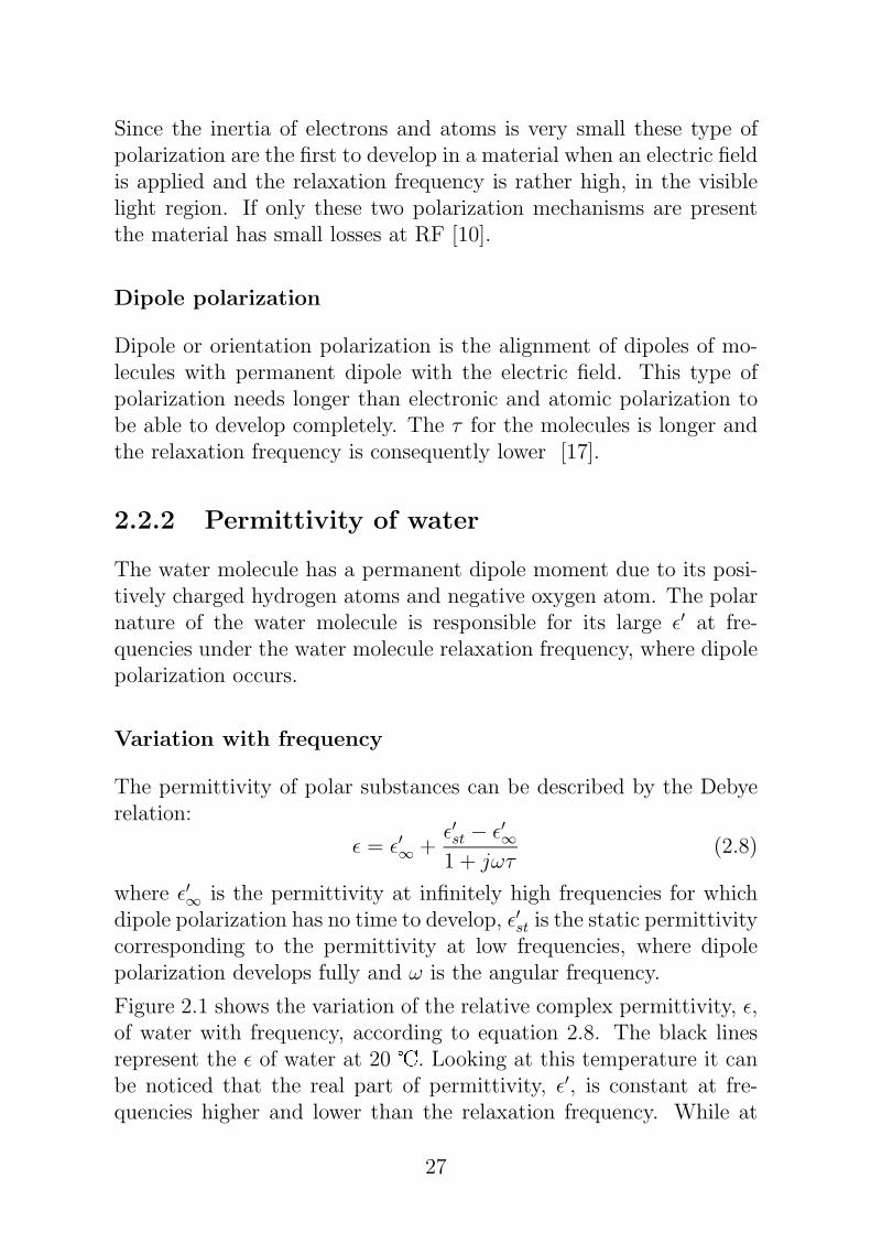
Figure 2.1 shows the variation of the relative complex permittivity, ǫ,of water with frequency, according to equation 2.8. The black linesrepresent the ǫ of water at 20 �. Looking at this temperature it canbe noticed that the real part of permittivity, ǫ′, is constant at fre-quencies higher and lower than the relaxation frequency. While at

27

108

109

1010

1011

10

20

30

40

50

60

70

80

frequency Hz

ε

ε’ 0°Cε’’ 0°Cε’ 20°Cε’’ 20°Cε’ 60°Cε’’ 60°C

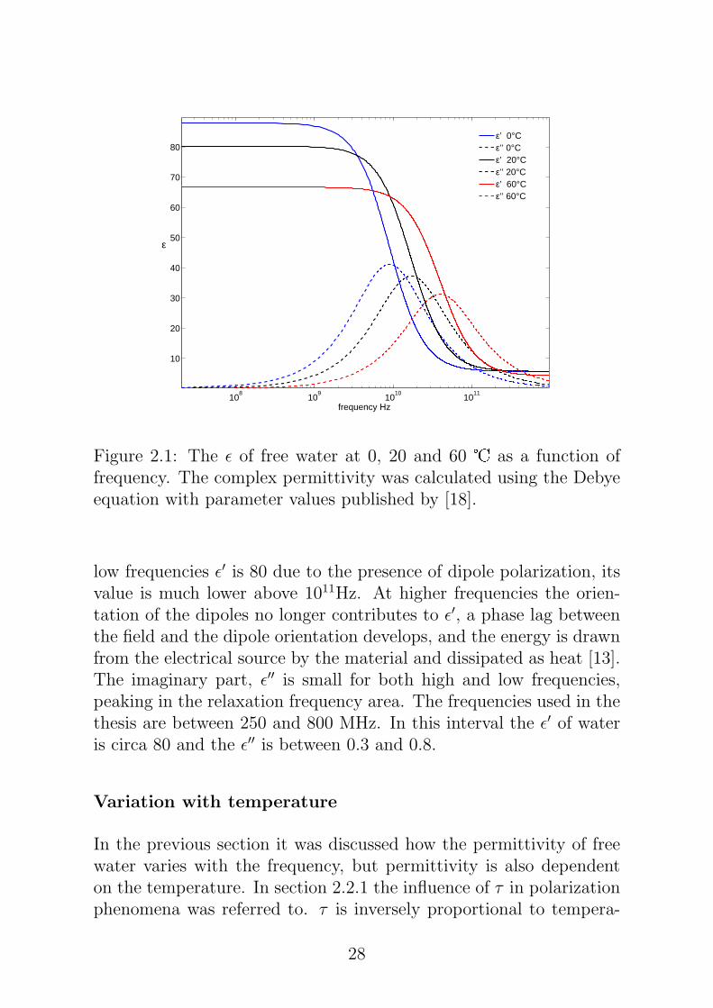
Figure 2.1: The ǫ of free water at 0, 20 and 60 � as a function offrequency. The complex permittivity was calculated using the Debyeequation with parameter values published by [18].

low frequencies ǫ′ is 80 due to the presence of dipole polarization, itsvalue is much lower above 1011Hz. At higher frequencies the orien-tation of the dipoles no longer contributes to ǫ′, a phase lag betweenthe field and the dipole orientation develops, and the energy is drawnfrom the electrical source by the material and dissipated as heat [13].The imaginary part, ǫ′′ is small for both high and low frequencies,peaking in the relaxation frequency area. The frequencies used in thethesis are between 250 and 800 MHz. In this interval the ǫ′ of wateris circa 80 and the ǫ′′ is between 0.3 and 0.8.

Variation with temperature

In the previous section it was discussed how the permittivity of freewater varies with the frequency, but permittivity is also dependenton the temperature. In section 2.2.1 the influence of τ in polarizationphenomena was referred to. τ is inversely proportional to tempera-

28

ture since molecular movement is faster at higher temperatures. Anincrease in temperature decreases the relaxation time and the relax-ation frequency is changed to a higher frequency. In figure 2.1 the ǫ′

of water at 0, 20 and 60 � are plotted using the values for τ , ǫ′∞

andǫ′st

published by [18]. It can be noted that an increase in temperaturemoves the fall of ǫ′ and the peak of ǫ′′ to the right. Temperatureinfluences not also the relaxation time but also static permittivity, ǫ′

st

which decreases with rising temperature. A higher temperature leadsto an increase in molecular disorder, which makes dipole polarizationmore difficult.

2.2.3 Permittivity of wood

Variation with frequency

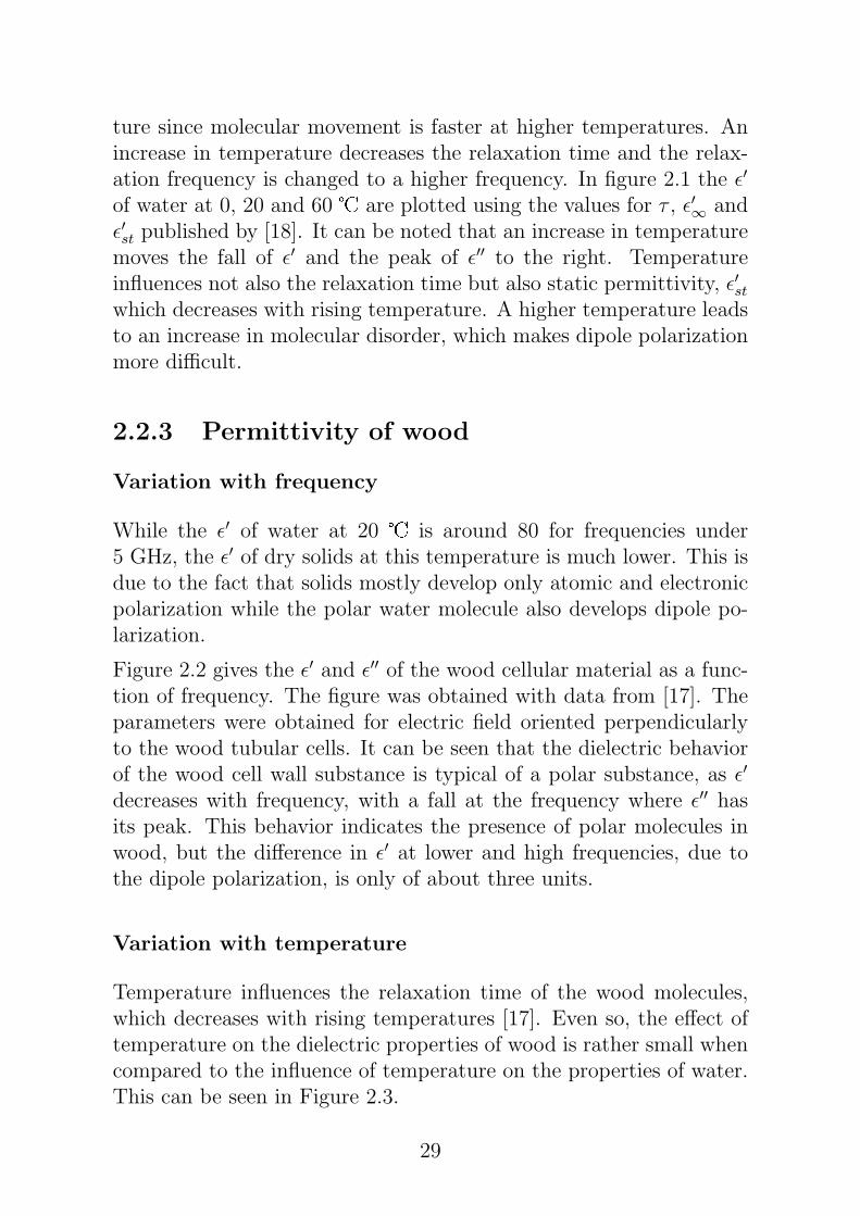
While the ǫ′ of water at 20 � is around 80 for frequencies under5 GHz, the ǫ′ of dry solids at this temperature is much lower. This isdue to the fact that solids mostly develop only atomic and electronicpolarization while the polar water molecule also develops dipole po-larization.

Figure 2.2 gives the ǫ′ and ǫ′′ of the wood cellular material as a func-tion of frequency. The figure was obtained with data from [17]. Theparameters were obtained for electric field oriented perpendicularlyto the wood tubular cells. It can be seen that the dielectric behaviorof the wood cell wall substance is typical of a polar substance, as ǫ′

decreases with frequency, with a fall at the frequency where ǫ′′ hasits peak. This behavior indicates the presence of polar molecules inwood, but the difference in ǫ′ at lower and high frequencies, due tothe dipole polarization, is only of about three units.

Variation with temperature

Temperature influences the relaxation time of the wood molecules,which decreases with rising temperatures [17]. Even so, the effect oftemperature on the dielectric properties of wood is rather small whencompared to the influence of temperature on the properties of water.This can be seen in Figure 2.3.

29

102

104

106

108

1010

0

1

2

3

4

5

6

7

frequency Hz

ε

Figure 2.2: The ǫ of the wood cell wall substance at the tempera-ture 20-25 � as a function of frequency. Values are for electric fieldperpendicular to the wood tubular cells and published by [17].

2.2.4 Permittivity of moist wood

Hydrogen atoms in the water molecule tend to form hydrogen boundsbetween themselves and with other molecules. When water is addedto a solid it forms bounds with the surface molecules of the solidphase. The hydrogen bounds restrict the movement of the watermolecules and decrease its ǫ′. Wood has a very large internal surfacedue to its fibrous structure. This high surface area is able to bind largequantities of water. Torgovnikov [17] defines the wood fiber saturationpoint as the point where all the water in wood cells is bound. Beyondthis point all water is kept inside cell cavities by mechanical forcesonly. For most wood species the mean value generally accepted forthe fiber saturation point is equivalent to a mass of water of 30% ofthe dry mass [17].

The permittivity of bound water varies with the material to which itis bound. The influence of frequency in the permittivity of a mixturewith both bound and free water phase is more complex than theinfluence on the free water molecule described in 2.2.2.

In a material with both free and bound water phases, temperature

30

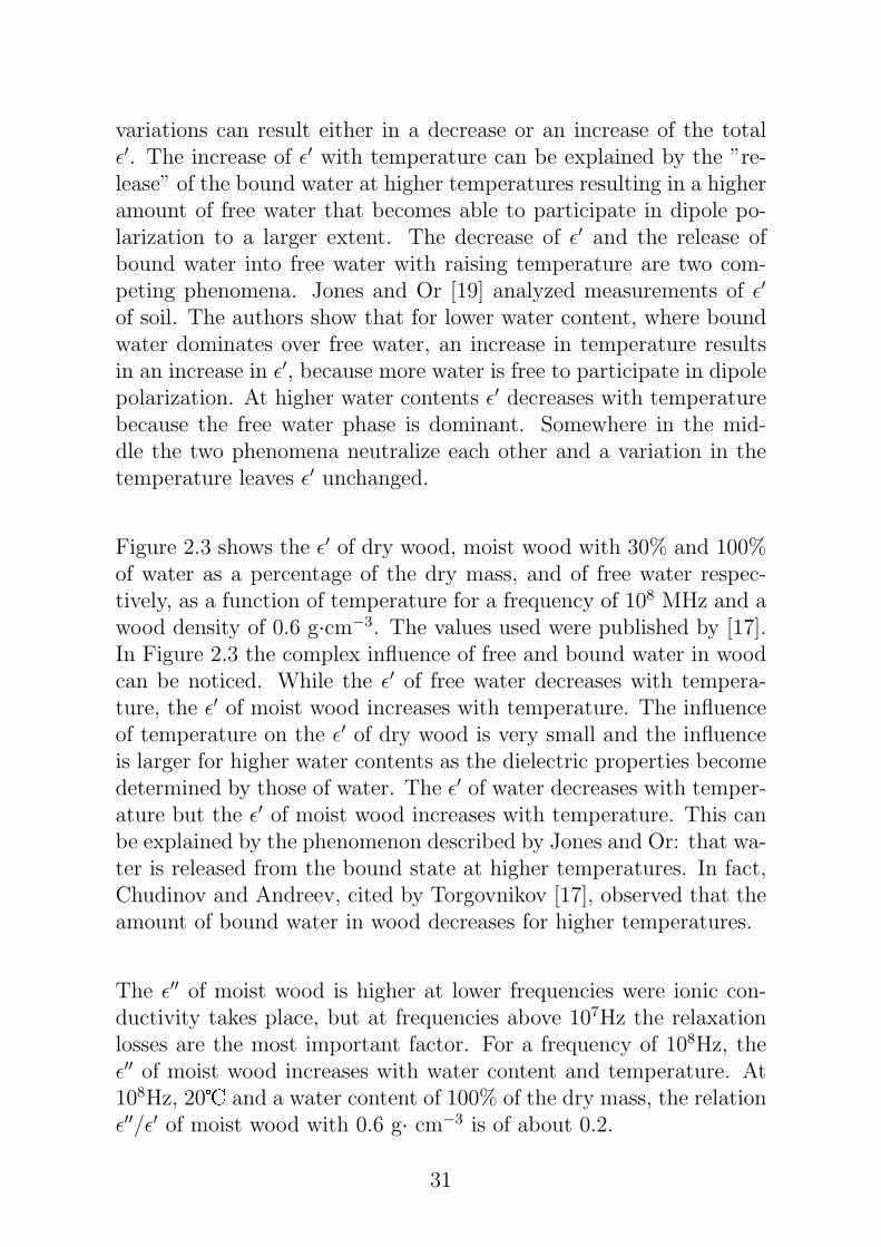
variations can result either in a decrease or an increase of the totalǫ′. The increase of ǫ′ with temperature can be explained by the ”re-lease” of the bound water at higher temperatures resulting in a higheramount of free water that becomes able to participate in dipole po-larization to a larger extent. The decrease of ǫ′ and the release ofbound water into free water with raising temperature are two com-peting phenomena. Jones and Or [19] analyzed measurements of ǫ′

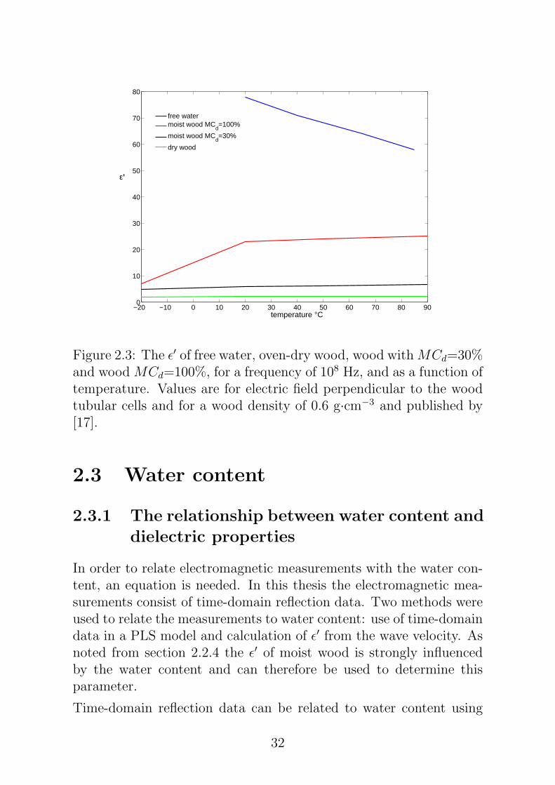
of soil. The authors show that for lower water content, where boundwater dominates over free water, an increase in temperature resultsin an increase in ǫ′, because more water is free to participate in dipolepolarization. At higher water contents ǫ′ decreases with temperaturebecause the free water phase is dominant. Somewhere in the mid-dle the two phenomena neutralize each other and a variation in thetemperature leaves ǫ′ unchanged.

Figure 2.3 shows the ǫ′ of dry wood, moist wood with 30% and 100%of water as a percentage of the dry mass, and of free water respec-tively, as a function of temperature for a frequency of 108 MHz and awood density of 0.6 g·cm−3. The values used were published by [17].In Figure 2.3 the complex influence of free and bound water in woodcan be noticed. While the ǫ′ of free water decreases with tempera-ture, the ǫ′ of moist wood increases with temperature. The influenceof temperature on the ǫ′ of dry wood is very small and the influenceis larger for higher water contents as the dielectric properties becomedetermined by those of water. The ǫ′ of water decreases with temper-ature but the ǫ′ of moist wood increases with temperature. This canbe explained by the phenomenon described by Jones and Or: that wa-ter is released from the bound state at higher temperatures. In fact,Chudinov and Andreev, cited by Torgovnikov [17], observed that theamount of bound water in wood decreases for higher temperatures.

The ǫ′′ of moist wood is higher at lower frequencies were ionic con-ductivity takes place, but at frequencies above 107Hz the relaxationlosses are the most important factor. For a frequency of 108Hz, theǫ′′ of moist wood increases with water content and temperature. At108Hz, 20� and a water content of 100% of the dry mass, the relationǫ′′/ǫ′ of moist wood with 0.6 g· cm−3 is of about 0.2.

31

−20 −10 0 10 20 30 40 50 60 70 80 900

10

20

30

40

50

60

70

80

temperature °C

ε’

free watermoist wood MC

d=100%

moist wood MCd=30%

dry wood

Figure 2.3: The ǫ′ of free water, oven-dry wood, wood with MCd=30%and wood MCd=100%, for a frequency of 108 Hz, and as a function oftemperature. Values are for electric field perpendicular to the woodtubular cells and for a wood density of 0.6 g·cm−3 and published by[17].

2.3 Water content

2.3.1 The relationship between water content and

dielectric properties

In order to relate electromagnetic measurements with the water con-tent, an equation is needed. In this thesis the electromagnetic mea-surements consist of time-domain reflection data. Two methods wereused to relate the measurements to water content: use of time-domaindata in a PLS model and calculation of ǫ′ from the wave velocity. Asnoted from section 2.2.4 the ǫ′ of moist wood is strongly influencedby the water content and can therefore be used to determine thisparameter.

Time-domain reflection data can be related to water content using

32

multivariate data analysis methods such as partial least square regres-sion (PLS). In this case the reflection coefficients at different timesare the independent variables. PLS is able to predict one or a set ofdependent variables from a large set of independent variables. It com-bines principal components analysis and multiple regression. Whileprincipal component analysis finds the orthogonal linear combinations(latent variables) of the dependent variables in order to explain thevariance in this set, PLS finds the latent variables that have maxi-mum correlation with the dependent variable set [20]. PLS has beenused to relate time-domain RF signal with the water content of woodybiomass [7].

The relation between ǫ′ and water content can be established by statis-tical or physical models. An example of a statistical equation relatingǫ′ to water content is Topp’s equation derived for prediction of soilwater content [15]. This equation has been found to predict watercontent in soil and other porous materials accurately and is widelyused [21, 22, 23]. It is also possible to make use of physically basedmodels, such as mixing models. These models are based on the as-sumption that the dielectric properties of a mixture are a function ofthe dielectric properties of the individual components of the mixture,their fractional volumes, and on polarization effects dependent on theshape of the components, as expressed in equation (2.9):

ǫ′m

= f(I

∑

i=1

(ǫ′i, θi, Dpi)) (2.9)

where ǫ′m

is the relative dielectric constant of the mixture, ǫ′iis relative

dielectric constant of the component i, θi is the volumetric content ofthe component i and Dpi accounts for the particle shape in componenti. Empirical parameters are incorporated into some mixing models inorder to improve their performance in practical applications, whereasothers have a purely theoretical basis. Theoretical mixing models arevaluable for improving our understanding of the dielectric behaviorof the mixture [16]. Mixing models have been applied to describe thedielectric behavior of different materials such as soil [24, 25], granularmaterials [23, 26], snow and ice [27, 28].

33

2.3.2 Reference water content

The reference method for determining the water content in woodybiomass is the standard gravimetric method. This method consists offirst weighing a sample of the material, drying the sample in an ovenand then weighing the dry material. The weight difference betweenthe wet and dry material is considered to be the mass of water in thesample. This method is fully described in the standard [29].

The application of the reference method requires sampling of the ma-terial whose water content is to be determined. The procedure forsampling woody biomass for water content determination with thestandard oven method is described in the standard [30].

2.3.3 Water content definitions

There are different definitions of water content depending on the wayin which this parameter is calculated. Water content can be calculatedon a volumetric basis. This is called volumetric water content orvolumetric water fraction, θw, and it is calculated according to 2.10:

θw =Vw

Vt

[m3 · m−3] (2.10)

where Vw is the volume of water and Vt is the total volume. Watercontent can also be calculated on a gravimetric basis. In this case itcan be defined as the mass of water, Mw as percentage of the totalmass of the sample, Mt, as shown in equation 2.11 or as a percentage ofthe mass of dry matter in the sample, Ms, according to equation 2.12:

MCw =Mw

Mt

· 100 [%] (2.11)

MCd =Mw

Ms

· 100 [%] (2.12)

MCd is a useful definition when the analysis is related with theamount of bound water. The amount of bound water in wood de-pends on the amount of dry matter. The generally accepted value for

34

the maximum amount of bound water in wood MCd= 30% [17]. Toverify the amount of bound and free water in a sample it is thereforeimportant to express the water content as a percentage of the drymatter.

θw is the most used definition when studying the dielectric behaviorof moist mixtures. ǫ′

mis better explained as a function of the volu-

metric content than as a function of the gravimetric content of theconstituents due to bulk density effects. This is shown, for instance,by Hallikainen et al. [31] for ǫ′

mof soil against θw and MCw.

MCw is a widely used definition of water content and probably theone whose value can be perceived most directly. The standard ovenmethod for water content gives results in gravimetric units and inmany cases it is not possible to calculate the volumetric content withthe same accuracy due to difficulties in volume measurement. It ispossible to calculate θw from MCw using the relation in 2.13:

θw =MCw

100·

ρt

ρw

[%] (2.13)

where ρt is the density of the sample calculated as Mt/Vt and ρw isthe water density.

2.4 Measurement systems

Dielectric properties can be measured accurately using different labo-ratory methods, but not all of them are adequate when measurementsoutside laboratory conditions are required. Examples of measure-ments outside laboratory conditions are, for instance, the measure-ment of soil or a crop canopy directly in the field and measurementsof materials in an industrial line. These applications often requirethat the materials are measured without touching or destroying them.They also require a set-up that is able to measure in a range of situa-tions that may imply moving the material, measuring a large portionof the material and measurements in different kinds of sample holders.

Several microwave and RF systems have been developed to measurewater content on-line in materials such as grain, powders, foodstuffs

35

or mineral ore. A review of these can be found in [6, 32]. However,these methods cannot measure large volumes of material. A materialwhose measurement demands can be compared with the bulk mea-surement of woody biomass in containers is soil. The measurement ofwater content in soil in-field is of great importance in fields like agri-culture, hydrology or civil engineering. Therefore several studies havebeen done within this area. A successfully developed technique hasbeen time domain reflectromety, TDR. TDR makes use of the wavevelocity in a transmission line inserted in the soil to determine soilwater content and uses the attenuation to determine soil conductiv-ity [33]. TDR probes are limited to measurements of volumes up to 1dm3 [34]. Ground penetrating radar, GPR, has been used to measurewater content in larger areas of soil [35]. Several methods are usedin soil water content measurements with GPR. When the depth toa reflector, such as a water table, is known, the travel time to thatreflector can be used to calculate the velocity of the waves in soil. ǫ′

can be calculated and correlated with the average water content inthe zone before the reflector. Stoffregen et al. [36] used this methodto determine average water content at a soil depth of 1.5 m.

The calibration models and the prediction results can be evaluatedand compared by calculating the root mean square error, RMSE,according to equation (2.14):

RMSE =

√

√

√

√

N∑

n=1

(ymeas − ymod)2

N(2.14)

where N is total the number of samples, ymeas is the measured pa-rameter and ymod is the parameter calculated with the model. TheRMSE is commonly named root mean square error of the calibrationwhen calculated with samples used to build a model, and root meansquare error of prediction when it is calculated with an independentset of samples.

36

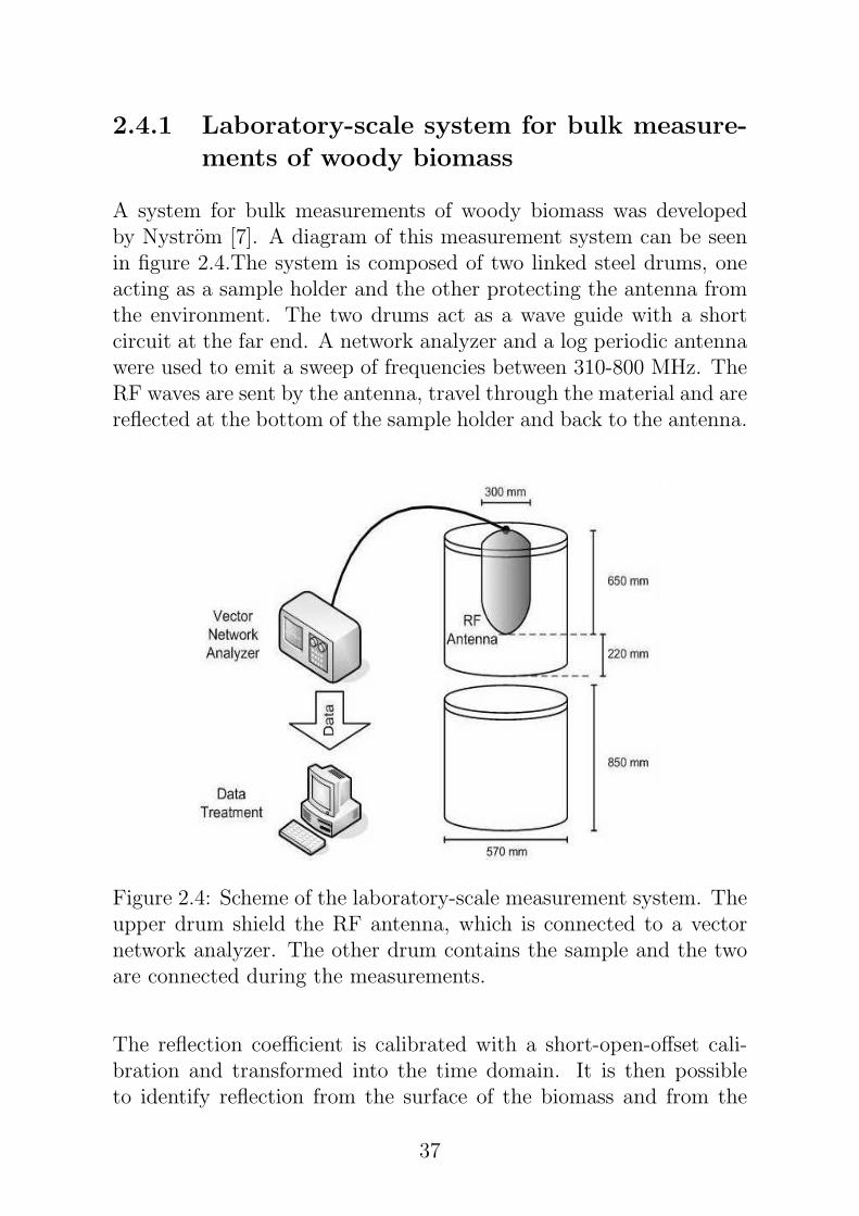
2.4.1 Laboratory-scale system for bulk measure-

ments of woody biomass

A system for bulk measurements of woody biomass was developedby Nystrom [7]. A diagram of this measurement system can be seenin figure 2.4.The system is composed of two linked steel drums, oneacting as a sample holder and the other protecting the antenna fromthe environment. The two drums act as a wave guide with a shortcircuit at the far end. A network analyzer and a log periodic antennawere used to emit a sweep of frequencies between 310-800 MHz. TheRF waves are sent by the antenna, travel through the material and arereflected at the bottom of the sample holder and back to the antenna.

Figure 2.4: Scheme of the laboratory-scale measurement system. Theupper drum shield the RF antenna, which is connected to a vectornetwork analyzer. The other drum contains the sample and the twoare connected during the measurements.

The reflection coefficient is calibrated with a short-open-offset cali-bration and transformed into the time domain. It is then possibleto identify reflection from the surface of the biomass and from the

37

bottom of the container. The travel time through the sample can beobtained by the difference between the times of the reflections at thebottom and at the biomass surface. The velocity of the RF waves inbiomass can be calculated using the travel time and the height of thesample using equation (2.7). A detailed description of the system canbe found in [37].

Water content in woody biomass with this system has been predictedusing a statistical model built with PLS, obtaining a RMSE of pre-diction of about MCw=2.7% [7].

38

Chapter 3

Contributions of the thesis

In this chapter the contributions of each paper included in this thesisare presented. A resume of the aim, methods, results and conclusionsare also presented. The aim is to give a comprehensive view of thework done within each of the three papers.

The following main contributions of the thesis can be listed:

- Evaluation of the influence of temperature on the ǫ′m

and watercontent measurements of woody biomass within the 1-62 � range(Paper I ).

- Analysis of the behavior of the ǫ′m

of woody biomass and develop-ment of a semi-physical model that is able to describe this behavior(Paper II ).

- Test the use of ǫ′m

to predict water content in woody biomass (PaperII ).

- Full-scale measurement of ǫ′m

of woody biomass (Paper III ).

3.1 Influence of temperature in the ǫ′m of

woody biomass

The variation of ǫ′ with temperature in water, wood and moist woodwas discussed in Chapter 2. The influence of temperature in a mixturewith both bound and free water phases is complex and difficult to

39

predict because it depends on the water content and on the degreeof binding. Therefore studying the influence of temperature in ǫ′

mof

woody biomass was of interest.

In Paper I the study of the influence of temperature in dielectricmeasurements of water content in woody biomass is presented. Theinfluence of temperature was investigated by performing a total ofsixty measurements of six different biomass samples at different tem-peratures. The MCw of the samples varied between 31% and 63%,which correspondent to a MCd between 46 and 167%. Measurementswere made with temperatures varying from 1 to 62 �. The followingprocedures were used in the analysis of the results:

- Study of the travel time and attenuation for different sample tem-peratures;

- Principal component analysis of the data;

- Evaluation of the prediction ability for an independent validation setwith varying temperatures using a model built with samples measuredat room-temperature only.

3.1.1 Results and discussion

The results presented in Paper I show that variations in attenuationand travel time of the signal can occur for the same sample, but itwas not possible to correlate these variations with the temperature.

In the multivariate data analysis it was noticed that it is not possibleto identify temperature in the score plot with the principal compo-nents that describe the data set.

The validation with independent test sets show that using sampleswith different temperatures does not seem to affect the predictionability of a model calibrated with samples at room-temperature.

In Figure 3.1, ǫ′m

calculated from the travel time of the samples ispresented as a function of temperature for the six samples used in thestudy. It can be noticed that for samples with same water content, ǫ′

m

can vary for different sample temperatures. However this variation israther small and it is not possible to detect a trend in these variationrelated with the sample temperature. In Figure 2.3 it is possible to

40

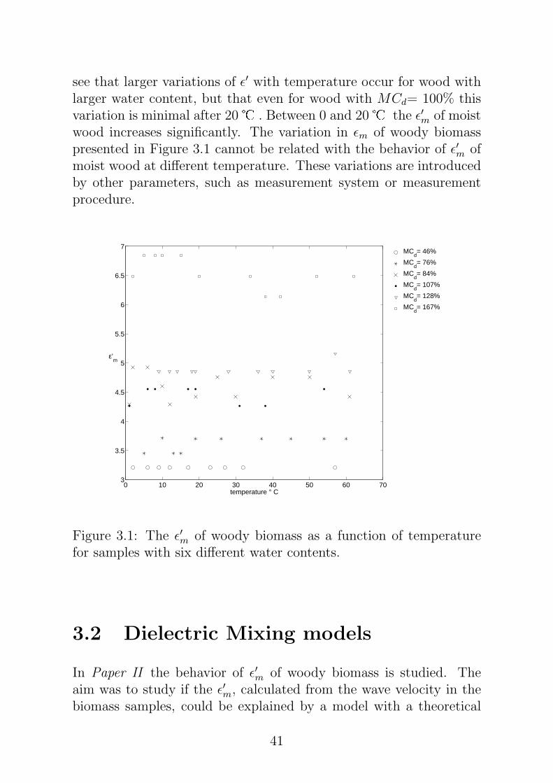
see that larger variations of ǫ′ with temperature occur for wood withlarger water content, but that even for wood with MCd= 100% thisvariation is minimal after 20� . Between 0 and 20� the ǫ′

mof moist

wood increases significantly. The variation in ǫm of woody biomasspresented in Figure 3.1 cannot be related with the behavior of ǫ′

mof

moist wood at different temperature. These variations are introducedby other parameters, such as measurement system or measurementprocedure.

0 10 20 30 40 50 60 703

3.5

4

4.5

5

5.5

6

6.5

7

temperature ° C

ε’m

MC

d= 46%

MCd= 76%

MCd= 84%

MCd= 107%

MCd= 128%

MCd= 167%

Figure 3.1: The ǫ′m

of woody biomass as a function of temperaturefor samples with six different water contents.

3.2 Dielectric Mixing models

In Paper II the behavior of ǫ′m

of woody biomass is studied. Theaim was to study if the ǫ′

m, calculated from the wave velocity in the

biomass samples, could be explained by a model with a theoretical

41

basis and verify that such a model can be used to predict water contentin the mixture.

Understand the relation between dielectric measurements and watercontent is important to the development of measurement systems.A calibration model based on ǫ′

mcould be applied in systems with

different equipment, set-up or different sample sizes.

The dielectric behavior of biomass was studied using dielectric mixingmodels. These models make use of the volumetric fractions, ǫ′, andthe geometry of each constituent of the mixture to determine the ǫ′

m.

ǫ′m

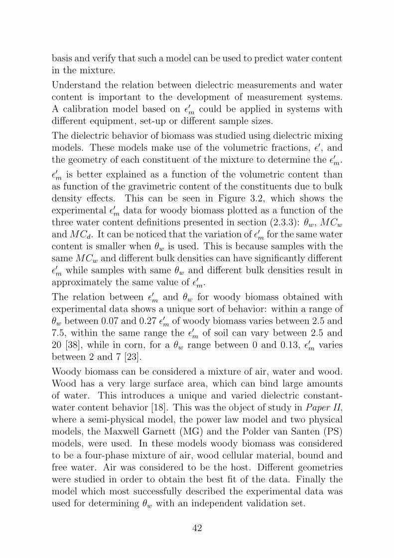
is better explained as a function of the volumetric content thanas function of the gravimetric content of the constituents due to bulkdensity effects. This can be seen in Figure 3.2, which shows theexperimental ǫ′

mdata for woody biomass plotted as a function of the

three water content definitions presented in section (2.3.3): θw, MCw

and MCd. It can be noticed that the variation of ǫ′m

for the same watercontent is smaller when θw is used. This is because samples with thesame MCw and different bulk densities can have significantly differentǫ′m

while samples with same θw and different bulk densities result inapproximately the same value of ǫ′

m.

The relation between ǫ′m

and θw for woody biomass obtained withexperimental data shows a unique sort of behavior: within a range ofθw between 0.07 and 0.27 ǫ′

mof woody biomass varies between 2.5 and

7.5, within the same range the ǫ′m

of soil can vary between 2.5 and20 [38], while in corn, for a θw range between 0 and 0.13, ǫ′

mvaries

between 2 and 7 [23].

Woody biomass can be considered a mixture of air, water and wood.Wood has a very large surface area, which can bind large amountsof water. This introduces a unique and varied dielectric constant-water content behavior [18]. This was the object of study in Paper II,where a semi-physical model, the power law model and two physicalmodels, the Maxwell Garnett (MG) and the Polder van Santen (PS)models, were used. In these models woody biomass was consideredto be a four-phase mixture of air, wood cellular material, bound andfree water. Air was considered to be the host. Different geometrieswere studied in order to obtain the best fit of the data. Finally themodel which most successfully described the experimental data wasused for determining θw with an independent validation set.

42

0 0.2 0.42

3

4

5

6

7

8

θw [m3.m−3]

ε’m

20 40 60 802

3

4

5

6

7

8

MCw [%]

ε’m

0 100 2002

3

4

5

6

7

8

MCd [%]

ε’m

Figure 3.2: The ǫ′m

of woody biomass as a function of different watercontent definitions: θw, MCw and MCd. It can be noticed that thedispersion is smaller when θw is used.


It was found that the MG model was able to describe the behavior ofǫ′m

of woody biomass. This model was obtained using disc-like geom-etry for the bound water inclusions and oblate ellipsoidal geometryfor the free water inclusions. These geometries resulted in the bestfit of the experimental data. It was found that the influence of thegeometry of wood cellular material inclusions can be neglected, as theθ and ǫ′ of this phase are rather small. Although the MG model wasable to explain satisfactorily the trend in the experimental data, itis difficult to base the results of the best fitting geometries on thestructure of the biomass constituents. In this manner the resultantmodel is a semi-physical model, as some parameters were obtained byfitting and lack justification in physical characteristics.

The use of this model with an independent validation set for predic-

43

tion of volumetric water content results in a RMSE of 0.029 m3·m−3.This result is on the same order as prediction error results foundin soil water content measurements [34]. However, when using themean density of the biomass samples to convert the error to gravi-metric units, according to equation (2.13), a RMSE of prediction ofMCw=8.9% is obtained. This is a larger error than using multivariatedata analysis to predict water content, as was done in Paper I, wherethe highest RMSE of prediction obtained was MCw=2.6%.

3.3 Full-scale measurements

Paper III describes results from full-scale RF measurements of woodybiomass, which entails that measurements were made directly in thecontainers where the biomass is transported. Figure 3.3 shows a pic-ture of the GPR antenna placed on the surface of the biomass. Theset-up that holds the antenna and moves it along the biomass surfaceis also visible. A detailed description of the set-up can be found in[8].

The biomass deliveries measured had a volume of about 100 m3 whilein the laboratory-scale method the samples had a volume of about 0.1m3. The full-scale system measures the entire depth of material in acontainer and the reference value obtained from the standard gravi-metric oven method is not representative of volume measured withRF. For this reason it was important to use the laboratory-scale mea-surements as a comparison. In Paper II ǫ′

mfor the laboratory-scale

measurements was calculated from the velocity of the waves in thesample and its behavior was explained based on a theoretical model.In Paper III, ǫ′

mis calculated in the same manner and compared with

results from laboratory-scale measurements.

It was shown in section (3.2) that ǫ′m

was better correlated with θw

than with gravimetric water content. Nevertheless, when studyingfull-scale results the correlation between ǫ′

mand θw was worse than

the one between ǫ′m

and MCw. This is probably due to the estimationof the total volume of the material, which is used to calculate θw

from the gravimetric reference value, as seen in equation 2.13. Thisestimation is not very accurate and might introduce random errors in

44

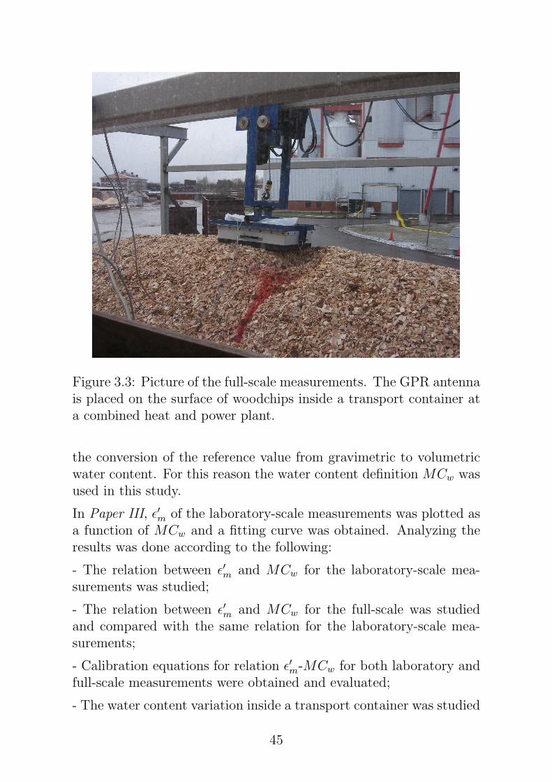
Figure 3.3: Picture of the full-scale measurements. The GPR antennais placed on the surface of woodchips inside a transport container ata combined heat and power plant.

the conversion of the reference value from gravimetric to volumetricwater content. For this reason the water content definition MCw wasused in this study.

In Paper III, ǫ′m

of the laboratory-scale measurements was plotted asa function of MCw and a fitting curve was obtained. Analyzing theresults was done according to the following:

- The relation between ǫ′m

and MCw for the laboratory-scale mea-surements was studied;

- The relation between ǫ′m

and MCw for the full-scale was studiedand compared with the same relation for the laboratory-scale mea-surements;

- Calibration equations for relation ǫ′m

-MCw for both laboratory andfull-scale measurements were obtained and evaluated;

- The water content variation inside a transport container was studied

45

by taking samples from different parts of the biomass tipped on theground.


The relation between ǫ′m

and MCw in the full-scale measurementsshows agreement with the same relation in laboratory-scale measure-ments. Both fitting curves follow the same trend but the dispersionis larger for full-scale measurements. This result indicates that acalibration model obtained with accurate reference values with thelaboratory-scale measurements could be used to predict the watercontent in the full-scale measurements.

Multiple measurements in a delivery of biomass tipped on the groundgave a maximum variation of 11% in MCw and a maximum standarddeviation of 5.6.

The RMSE for the calibration curves was 4.5% for the laboratory-scale calibration curve and 7.3% for the full-scale. The larger errorin the full-scale situation might be due to the large depth of materialand the open-air setup. This could also be due to inaccuracy in thefull-scale reference value which would mean a smaller actual error.

The RMSE value obtained with the fitting curve between ǫ′m

andMCw for full-scale measurements is rather large. Different methods,such as PLS, should be tested to investigate if it is possible to obtainbetter results with the woody biomass bulk measurement system.

46

Chapter 4

Conclusions

The conclusions are stated according to the four questions defined inthe beginning of the thesis:

Concerning the influence of temperature on ǫ′m

of woody biomass,it was found that it is not possible to associate variations in ǫ′

mwith

temperature variations. It was also shown that temperature variationswithin 1 and 62� did not influence the water content prediction errorwhen using a PLS model calibrated only with samples measured atabout 20 �.

Concerning the behavior of ǫ′m

of woody biomass, this could be ex-plained using the MG model, by assuming that woody biomass is anisotropic mixture of air, wood cellular material, free and bound water.However, the depolarization factors, used in the model to account forthe geometry of the inclusions, were obtained by statistical fittingand results were found to be difficult to base on physical biomasscharacteristics.

The prediction of water content with the MG model which was able todescribe the experimental data, obtained a RMSE of 0.029 m3·m−3.This error is larger than the prediction error obtained when PLS isused as a calibration model.

In the full-scale measurements an empirical model relating ǫ′m

withthe MCw obtained resulted in a RMSE of calibration of 7.3%. Thisvalue is obtained when using values from the oven reference method,which might not be accurate. The relation between ǫ′

mof biomass

and MCw followed the same trend in full-scale measurements as inlaboratory-scale measurements, although with a larger dispersion.

47

Chapter 5

Future work

This thesis concentrated on the study of the dielectric constant ofwoody biomass and its use in water content prediction. Althoughthis study is important to understanding the dielectric behavior ofwoody biomass, the use of the dielectric constant to predict watercontent resulted in larger prediction errors than when using PLS mod-els. Further analysis of the full-scale measurements has to be carriedout, namely using PLS methods, to verify if it is possible to obtainedsmaller prediction errors.

PLS models account for the attenuation in the material since thereflection coefficient data in time-domain is used. It is possible thatPLS models give better water content prediction due to this fact,which raises the interest in studying the ǫ′′ of woody biomass.

Another challenge is the possibility of measuring other biomass char-acteristics using the dielectric properties at radio frequencies. An ex-ample of an interesting parameter when woody biomass is used as afuel, is the ash content, in other words the nonvolatile inorganic mat-ter which remains after the combustion. Determining the inorganiccontent in biomass can be related with the electrical conductivity.The measurement of electrical conductivity with RF has also been asuccessfully achieved using TDR in soils.

49

Bibliography

[1] Biomass action plan. European Commission, 2005.

[2] Energy in sweden, figures and facts. Swedish Energy Agency,2007.

[3] J Nystrom and E Dahlquist. Methods for determination of mois-ture content in woodchips for power plants - a review. Fuel,83(7-8):773 – 779, 2004.

[4] L Axrup, K Markides, and T Nilsson. Using miniature diode ar-ray NIR spectrometers for analyzing woodchips and bark samplesin motion. Journal of Chemometrics, 14:561–572, 2000.

[5] Barale P, Fong C, Green M, Luft P, Mcinturff A, Reimer J, andYahnke M. The use of a permanent magnet for water contentmeasurements of wood chips. IEEE transactions on applied su-perconductivity, 12(1):975–978, 2002.

[6] S Okamura. Microwave technology for moisture measurement.Subsurface Sensing Technologies and Applications, 1(2):205–227,2000.

[7] J Nystrom. Rapid measurements of the moisture content in bio-fuel. PhD thesis, Malardalen Univeristy, 2006.

[8] A Paz, J Nystrom, and E Dahlquist. Water content measurementof biofuel with RF directly in trailers truck containers. Technicalreport, Varmeforsk, in manuscript.

[9] L Chen, C Ong, C Neo, V V Varadan, and V K Varadan.Microwave electronics, measurement and materials characteri-zation. Wiley, 2004.

51

[10] E Nyfors and P Vainikainen. Industrial Microwave Sensors.Artech House, 1994.

[11] A Hippel. Dielectric materials and applications: papers bytwenty-two contributors. Technology Press of M.I.T and Wiley,New York, 1954.

[12] F Ulaby. Fundamentals of applied electromagnetics. PearsonPrentice Hall, 5 edition, 2007.

[13] J Hasted. Aquous Dielectrics. Chapman and Hall, 1973.

[14] D Cheng. Field and wave electromagnetics. Addison Wesley,1989.

[15] G Topp, J Davis, and A Annan. Electromagnetic determinationof soil water content: measurements in coaxial transmission lines.Water Resources Research, 16(3):574 – 582, 1980.

[16] D Robinson, S Jones, J Wraith, D Or, and S Friedman. A reviewof advances in dielectric and electrical conductivity measurementin soils using time domain reflectometry. Vadose Zone Journal,2(4):444–475, 2003.

[17] G Torgovnikov. Dielectric properties of wood and wood basedmaterials. Springer-Verlag, 1992.

[18] U Kaatze. Electromagnetic wave interaction with water andaqueous solutions. In Electromagnetic Aquametry. Springer,2005.

[19] S Jones and D Or. Modeled effects on permittivity measurementsof water content in high surface area porous media. Physica B:Condensed Matter, 338(1-4):284–290, 2003.

[20] H Abdi. Partial least squares (PLS) regression. In Encyclopediaof Social Sciences Research Methods. Sage, 2003.

[21] C Dirksen and S Dasberg. Improved calibration of time domainreflectometry soil water content measurements. Soil Science So-ciety of America Journal, 57(3):660 – 667, 1993.

52

[22] A Turesson. Water content and porosity estimated from ground-penetrating radar and resistivity. Journal of Applied Geophysics,58(2):99–111, 2006.

[23] M Vallone, A Cataldo, and L Tarricone. Water content estima-tion in granular materials by time domain reflectometry: A key-note on agro-food applications. In IEEE Instrumentation andMeasurement Technology Conference, pages 1091–5281, Warsaw,Poland, 2007.

[24] H Gong, Y Shao, J Liu, Q Hu, and W Tian. Improved model fordielectric behavior of moist saline soil. In Proceedings of the Inter-national Society for Optical Engineering, volume 6787, Wuhan,China, 2007.

[25] M Dobson, F Ulaby, M Hallikainen, and M El-Rayes. Microwavedielectric behaviour of wet soil. II dielectric mixing models. IEEETrans. Geosci. Remote Sens. (USA), GE-23(1):35 – 46, 1985.

[26] M Hilhorst, C Dirksen, F Kampers, and R Feddes. New dielectricmixture equation for porous materials based on depolarizationfactors. Soil Science Society of America Journal, 64(5):1581 –1587, 2000.

[27] M Hallikainen, F Ulaby, and M Aderlrazik. The dielectric be-haviour of snow in the 3 to 37 GHz range. In IGARSS ’84. Re-mote Sensing - From Research Towards Operational Use, pages169 – 174, Strasbourg, France, 1984.

[28] A Sihvola. Electromagnetic mixing formulas and applications.The Intitution of Electrical Engineers, 1999.

[29] SS187170. Biofuels and peat- determination of total moisture.Swedish Standard Institution, 1998.

[30] SS187113. Biofuels and peat - sampling. Swedish Standard In-stitution, 1999.

[31] M Hallikainen, F Ulaby, M Dobson, M El-Rayes, and L Wu.Microwave dielectric behavior of wet soil. I empirical models and

53

experimental observations. IEEE Transactions on Geoscienceand Remote Sensing, GE-23(1):25 – 34, 1985.

[32] K Lawrence and S Nelson. Radiofrequency sensing of mois-ture content in cereal grains. In Sensors Update, pages 377–391.Wiley-VCH, 2000.

[33] P Ferre and G Topp. Time-domain reflectometry techniques forsoil water content and electrical conductivity measurements. InSensors Update, pages 277–300. Wiley-VCH, 2000.

[34] J Huisman, C Sperl, W Bouten, and J Verstraten. Soil watercontent measurements at different scales: accuracy of time do-main reflectometry and ground-penetrating radar. Journal ofHydrology, 245(1-4):48–58, 2001.

[35] J Huisman, S Hubbard, J Redman, and A Annan. MeasuringSoil Water Content with Ground Penetrating Radar: A Review.Vadose Zone J, 2(4):476–491, 2003.

[36] H Stoffregen, T Zenker, and G Wessolek. Accuracy of soil watercontent measurements using ground penetrating radar: compar-ison of ground penetrating radar and lysimeter data. Journal ofHydrology, 267(3-4):201–206, 2002.

[37] J Nystrom and B Franzon. Radio frequency system for mea-suring characteristics of biofuels. In Proceedings of the IEEEInstrumentation and Measurement Technology Conference, Ot-tawa, Ontario, Canada, 2005.

[38] N Peplinski, F Ulaby, and M Dobson. Dielectric properties ofsoils in the 0.3-1.3GHz range. IEEE Transactions on Geoscienceand Remote Sensing, 33(3):803–807, 1995.

54

water content measurement in woody biomass using dielectric constant at radio frequencies

Documents